Lean Beam Management for New Radio

ERICSSON

Lean Beam Management for New Radio

Nawanit Kumar

Department of Electrical and Information TechnologyLund University

Supervisors: Stefan Höst, LTHThomas Svensson and Joachim Ramkull, Ericsson Lund

Examiner: Maria Kihl

August 19, 2020

Popular Science Summary

In this modern epoch, demand and growth of high-speed mobile broadband hasbeen surging at never seen before pace. Hence primarily, it is need for tether-less communication with high data rates which has led to need of migration fromFourth generation to Fifth generation of mobile communication rather than voicecalls. This leads to need for large radio bandwidth. Large bandwidth further leadsto use of millimeter wave spectrum to achieve better power efficiency. Need forbetter bandwidth efficiency leads to use of phased array antenna modules or mas-sive multiple input multiple output antenna system. The base station has multipleantennas in Fifth generation New Radio. Despite availability of many antennas,the base station is equipped only with a fixed set of steering vectors. These arecalled beams in New Radio. Each beam is pointing in a certain direction in space.To cover multiple user equipment in a single transmission is almost impossiblewhen the radiation is beam shaped unless they are in very close proximity.

Fifth generation New Radio is the new radio access technology developed bythe 3rd Generation Partnership Project for mobile communication network. Itis the global standard for the air interface of Fifth generation networks. Analogbeam-forming is a technique used widely in Fifth generation New Radio AccessNetwork to counter propagation effects between transmitter and receiver. In ana-log beam-forming, connected devices are individually tracked so that the com-munication with each device takes place on the best beam. This is called beammanagement. Beam management comes with an additional cost. For radio accessnetwork to track the device and use the best beam, devices must perform regu-lar measurements called channel sounding and estimation and report them to thebase station of the mobile network system. Hence, these measurements consumeair interface resources which are costly and scarce given the high traffic volumeand could otherwise be used for data. The challenge increases with increase in thenumber of connected users in a cell.

The thesis aims to investigate current implementation of downlink beam man-agement in New Radio high-band and propose better suggestions to minimise thesemeasurements while still achieving decent throughput and coverage with reducedinterference.

i

Abstract

The use of millimetre-wave frequencies in Fifth generation New Radio has lead tohigh path loss due to radio propagation environment. Simultaneously, high datarates is a must for current products due to high market demand. This requirementaccounts for efficient tracking of the best beam for the user equipment to stay con-nected to it. Current products at Ericsson use such methods of beam management.These methods call for regular measurements of beams which add up to overhead.Overhead reduction is an area that is being continuously researched. Through thisthesis, two algorithms are proposed with the aim to reduce overhead. First, byincreasing the periodicity of measurements. Second, by reducing the number ofnarrow beam measurements. These solutions are simulated by comparing over-all system throughput values from a selection of beams. Theoretical calculationshave also been done. Both these results are compared to see the effectiveness ofthe proposed solutions. Different use cases are taken into consideration such asstationary and/or mobile users. In review, it can be clearly seen that increasingperiodicity of channel sounding is a good way to decrease measurements and usethe resources for data instead. However, reducing narrow beam measurementswas not found to be an overall feasible algorithm as the system performance waspoor for uplink leading to degradation in downlink. Thus, increasing periodicityfor channel estimation in downlink can be applied to New Radio beam manage-ment scenarios in millimetre-wave high-band to yield better average cell downlinkthroughput as compared to current products.

iii

Acknowledgements

The thesis in the physical layer high band has been very enriching. It servedits purpose of increasing my knowledge by imparting hands on experience on theongoing pioneering technological advancements in the industry of Fifth Generation.I would like to thank Ericsson Lund for letting me write my thesis and providingme with all necessary resources for the same. Ericsson is known for its wide spectraof research and innovation and I found it to be true in ways greater than what Icould possibly imagine. This was well supported by the theoretical backgroundlearnt through my courses at Faculty of Engineering, Lund University. I wasvery happy to discover that the knowledge imparted to us at the university is incomplete sync with the current industry standards. I have been fortunate to besupported by knowledgeable and patient supervisors Stefan Höst at the universityand Thomas Svensson and Joachim Ramkull at Ericsson. I would like to expressgratitude towards my friendly manager Samir Drincic for giving constant support,motivation and guidance. I would also like to thank Ingvar Pålsson, Akram BinSediq and Joel Bill who has been kind to divulge their time in helping me onmy thesis. The successful completion of the thesis would not have been possiblewithout these valuable contributions.

v

Table of Contents

1 Introduction 11.1 Background . . . . . . . . . . . . . . . . . . . . . . . . . . . . . . . 11.2 Objective . . . . . . . . . . . . . . . . . . . . . . . . . . . . . . . . 21.3 Thesis Formulation . . . . . . . . . . . . . . . . . . . . . . . . . . . 21.4 Previous Work . . . . . . . . . . . . . . . . . . . . . . . . . . . . . 21.5 Limitations . . . . . . . . . . . . . . . . . . . . . . . . . . . . . . . 41.6 Layout . . . . . . . . . . . . . . . . . . . . . . . . . . . . . . . . . . 4

2 Evolution of 5G 52.1 5G NR . . . . . . . . . . . . . . . . . . . . . . . . . . . . . . . . . 52.2 Coexistence . . . . . . . . . . . . . . . . . . . . . . . . . . . . . . . 62.3 NR v/s LTE . . . . . . . . . . . . . . . . . . . . . . . . . . . . . . . 72.4 Enhanced transmission scheme . . . . . . . . . . . . . . . . . . . . . 82.5 Dynamic Duplex scheme . . . . . . . . . . . . . . . . . . . . . . . . 132.6 Multiple antenna transmission . . . . . . . . . . . . . . . . . . . . . 142.7 Ultra-lean design . . . . . . . . . . . . . . . . . . . . . . . . . . . . 18

3 Current standards and proposed solution 293.1 Baseline solutions . . . . . . . . . . . . . . . . . . . . . . . . . . . . 293.2 Proposed algorithms . . . . . . . . . . . . . . . . . . . . . . . . . . 30

4 Theoretical calculations 314.1 Transport Block Size (TBS) . . . . . . . . . . . . . . . . . . . . . . 314.2 Maximum throughput calculation . . . . . . . . . . . . . . . . . . . 334.3 Algorithm 1: Increasing periodicity of CSI-RS . . . . . . . . . . . . . 354.4 Algorithm 2: Decreasing CSI-RS measurements . . . . . . . . . . . . 37

5 Methodology 395.1 Proposed algorithms . . . . . . . . . . . . . . . . . . . . . . . . . . 395.2 Simulator overview . . . . . . . . . . . . . . . . . . . . . . . . . . . 395.3 Traffic models . . . . . . . . . . . . . . . . . . . . . . . . . . . . . . 405.4 Key Performance Index . . . . . . . . . . . . . . . . . . . . . . . . 415.5 Simulator parameters . . . . . . . . . . . . . . . . . . . . . . . . . . 435.6 Simulation procedure . . . . . . . . . . . . . . . . . . . . . . . . . . 45

vii

6 Results 476.1 Theoretical result for periodicity increase . . . . . . . . . . . . . . . 476.2 Algorithm 1: Increasing periodicity of CSI-RS . . . . . . . . . . . . . 486.3 Algorithm 2: Decreasing CSI-RS measurements . . . . . . . . . . . . 52

7 Future Scope 577.1 Summary . . . . . . . . . . . . . . . . . . . . . . . . . . . . . . . . 577.2 Future work . . . . . . . . . . . . . . . . . . . . . . . . . . . . . . . 58

References 59

viii

List of Figures

2.1 IMT-2020 new use cases . . . . . . . . . . . . . . . . . . . . . . . . 52.2 NR NSA network . . . . . . . . . . . . . . . . . . . . . . . . . . . . 72.3 NR Time-Frequency architecture for 100 MHz bandwidth and µ = 3 92.4 Time domain architecture in NR . . . . . . . . . . . . . . . . . . . . 102.5 Antenna-port structure in NR . . . . . . . . . . . . . . . . . . . . . 112.6 CSI-RS Antenna-port mapping . . . . . . . . . . . . . . . . . . . . 122.7 Duplex schemes . . . . . . . . . . . . . . . . . . . . . . . . . . . . . 132.8 Beam establishment and refinement - P1 and Outer loop P2 . . . . . 152.9 Beam refinement - Inner loop P2 . . . . . . . . . . . . . . . . . . . 172.10 Logical, transport, and physical channels mapping . . . . . . . . . . 182.11 PDSCH mapping . . . . . . . . . . . . . . . . . . . . . . . . . . . . 192.12 TDD 4+1 PHY data and control channel architecture . . . . . . . . 202.13 Time-frequency resources in TDD 4+1 . . . . . . . . . . . . . . . . 222.14 Two-port CSI-RS structure based on 2xCDM . . . . . . . . . . . . . 242.15 Multiple antenna-port CSI-RS mapping . . . . . . . . . . . . . . . . 252.16 CORESET with QCL . . . . . . . . . . . . . . . . . . . . . . . . . . 28

4.1 NR TBS calculation . . . . . . . . . . . . . . . . . . . . . . . . . . 32

5.1 Simulation layout with one cell and one gNB . . . . . . . . . . . . . 425.2 Straight mover . . . . . . . . . . . . . . . . . . . . . . . . . . . . . 45

6.1 Theoretical DL throughput varying P2 periodicity. Negative valuesshow all resources consumed for channel sounding. . . . . . . . . . . 47

6.2 Average Cell DL throughput with varying P2 periodicity (5km/hr) . . 486.3 Average Cell DL throughput with varying P2 periodicity (50km/hr) . 496.4 FTP DL throughput with varying P2 periodicity (5km/hr) . . . . . . 506.5 FTP DL throughput with varying P2 periodicity (100km/hr) . . . . . 506.6 Cell DL throughput comparison between 6 beams and 12 beams with

varying speed . . . . . . . . . . . . . . . . . . . . . . . . . . . . . . 526.7 Cell DL and UL throughput gain (5km/hr) . . . . . . . . . . . . . . 536.8 FTP DL throughput comparison between 6 beams and 12 beams with

varying speed . . . . . . . . . . . . . . . . . . . . . . . . . . . . . . 54

ix

6.9 FTP UL throughput comparison between 6 beams and 12 beams withvarying speed . . . . . . . . . . . . . . . . . . . . . . . . . . . . . . 54

6.10 FTP DL and UL throughput gain (5km/hr) . . . . . . . . . . . . . . 55

x

List of Tables

4.1 Throughput (Mbps) by varying P2 periodicity (ms) for different num-ber of users* . . . . . . . . . . . . . . . . . . . . . . . . . . . . . . 36

xi

List of Acronyms

3GPP Third Generation Partnership Project3D-UMa Three Dimesional Urban Macrocell4G Fourth Generation5G Fifth GenerationABF Analog BeamformingARQ Automatic Repeat-reQuestAWGN Additive White Gaussian NoiseBLER Block Error RatioBS Base StationCA Carrier AggregationCC Component CarrierCDM Coding and Modulation SchemeCE Control ElementCH Channel HardeningCORESET Control Resource SetCSI Channel State InformationCSI-IM CSI Interference MeasurementCSI-RS CSI Reference SignalCQI Channel Quality IndicatorDCI Downlink Control InformationDFT Discrete Fourier TransformDL DownlinkDM-RS Demodulation Reference SignalEKF Extended Kalman FiltereMBB enhanced MBBeNB eNodeBEN-DC E-UTRA NR Dual-ConnectivityEPA Extended Pedestrian A ModelEPC Evolved Packet Core

xiii

E-UTRA Evolved UTRAFDD Frequency Division DuplexFDM Frequency-Domain SharingFR1 Frequency Range 1FR2 Frequency Range 1FTP File Transfer ProtocolgNB gNodeBgNodeB generalized NodeBGSM Global System for Mobile CommunicationH-ARQ Hybrid ARQIEEE Institute of Electrical and Electronics EngineersIMT-2020 International Mobile Telecommunications 2020IoT Internet of ThingsITU-R ITU-Radio SectorITU International Telecommunications UnionKPI Key Performance IndexL1-RSRP Layer 1 RSRPLA Link adaptationLTE Long Term EvolutionLOS Line Of SightMAC Medium Access ControlMAC-CE MAC Control ElementMBB Mobile BroadbandMCS Modulation and Coding SchemeMIMO Multiple Input Multiple OutputML Machine LearningMTC Machine Type CommunicationmMTC massive MTCMU-MIMO Multi-User MIMOmmWave Millimeter WaveNLOS Non LOSNOMA Non-Orthogonal Multiple AccessNR New RadioNSA Non StandaloneNZP CSI-RS Non-zero-power CSI-RSOFDM Orthogonal Frequency-Division MultiplexingPAAM Phased Antenna Array ModulesPBCH Physical Broadcast ChannelPCCH Paging Control ChannelPDCCH Physical Downlink Control ChannelPDSCH Physical Downlink Shared ChannelPHY Physical LayerPRACH Physical Random-Access Channel

xiv

PRB Physical Resource BlockPT-RS Phase Tracking Reference SignalPUCCH Physical Uplink Control ChannelPUSCH Physical Uplink Shared ChannelPMI Precoder Matrix IndicatorQAM Quadrature Amplitude ModulationQCL Quasi Co-LocationQoS Quality-of-ServiceRACH Random Access ChannelRAN Radio Access NetworkRAT Radio Access TechnologyRB Resource BlockRE Resource ElementRI Rank IndicatorRIM Remote Interference ManagementRIM-RS RIM Reference SignalRLC Radio-Link ControlRRC Radio Resource ControlRRM Radio Resource ManagementRS Reference SymbolRSRP Reference Signal Received PowerRV Redundancy VersionSNR Signal-to-Noise RatioSRS Sounding Reference SignalSSB Synchronization Signal BlockSDAP Service Data Application ProtocolTBS Transport Block SizeTCI Transmission Configuration IndicationTCP Transmission Control ProtocolTDD Time-Division DuplexTDM Time Domain SharingTRP Transmission Reception PointTRS Tracking Reference SignalTTI Transmission Time IntervalUDP User Datagram ProtocolUE User EquipmentUL UplinkUMTS Universal Mobile Telecommunication SystemURLLC Ultra-reliable low-latency communicationUTRA Universal Terrestrial Radio AccessZP CSI-RS Zero-power CSI-RS

xv

Chapter1Introduction

1.1 Background

5G New Radio (NR) Radio Access Network (RAN) is expected to achieve veryhigh data rates of more than 1 Gigabits per second (Gbps) with Enhanced MobileBroadband (eMBB) according to Third Generation Partnership Project (3GPP)[14]. Looking at Ericsson’s mobility report, mobile data traffic has grown by 49percent between quarter 4 for 2018 and 2019 [34] to reach 6.3 billion mobile broad-band subscriptions globally. A total of 49 million subscriptions were added in justone quarter. 5G subscriptions are expected to reach 190 million by end of 2020[35]. This rapid traffic growth is caused by rising number of smartphone subscrip-tions and increasing average data volume per subscription. This is primarily dueto increase in video content usage. Rise in subscriptions is also due to increasein number of connected devices through Internet of Things (IoT). This demandleads to need for large radio bandwidth which further leads to use of millimetrewave (mmWave) spectrum for better power efficiency. Due to physics of natureof waves, transmitting a signal in all directions and/or at relatively wide anglesis possible for mid and low frequency range. In these cases, a single transmissionwould cover a lot of user equipment (UE) simultaneously without using massiveantenna array. Need for better bandwidth efficiency leads to use of phased antennaarray modules (PAAM) or massive multiple input multiple output (mMIMO) an-tenna system which further results in radiation being a beam. Beam is used forhigh frequency to cover multiple UE. However, mmWaves experience great prop-agation loss, especially for larger distances between transmitter and receiver andeven due to the atmospheric absorption by oxygen molecules and water vapor[33]. Channel conditions and radio link quality also changes significantly for mo-bile users. In order to counter this difficulty, a very sophisticated technique ofmanaging/controlling the beam to cover multiple devices scattered in all direc-tions is required. This control mechanism called beamforming should be genericenough to adapt to different scenarios.

Beamforming concentrates transmitted signal in receiver’s direction which im-proves received signal power. Analog Beamforming (ABF) is such a techniqueused widely in 5G NR RAN to counter propagation effects between transmitterand receiver [32]. In ABF, connected devices are individually tracked so that thecommunication with each device happens on the best beam. This is called beam

1

2 Introduction

management. Beam Management is a collection of techniques such as initial beamestablishment, beam refinement and beam tracking to refine directional links be-tween transmitter and receiver beams [29].

1.2 Objective

The aim of the thesis is to investigate the current standards of beam managementand beam tracking measurements applied in the industry as baseline solutions.Comprehensive study of recent ongoing work in this domain is done and based onthe cumulative knowledge of the above, new mechanisms of reducing measurementsof beam tracking are to be proposed and simulated. These proposed solutions arecompared with baseline solutions for their effectiveness.

1.3 Thesis Formulation

Beam management involves selecting the best beam for connection establishmentbetween the UE and the network or base station (BS). This is typically done bymeasuring Channel State Information Reference Signals (CSI-RS) of the candidatebeams [1]. More specifically, Reference Signal Received Power (RSRP) values ofthe candidate beams are measured and the one with highest value is selected asthe best beam. Ideally, this power will be highest where best possible channelquality is experienced. The standards on these channel reference signals is leftto be independently designed by the network provider by 3GPP [1]. Thus, thesemeasurements for best beam occur with a specific periodicity which is determinedby the network provider alone.

Minimising the number of reference measurements is vital so that majority oftime-domain resources are used for data and control information. This is even morecrucial in dense deployments for reducing power consumption. However, trying tooptimise and minimise all the parameters associated with beam management liesoutside the scope of the thesis. The problem formulation of the thesis was limitedto investigating effect of periodicity increase of CSI-RS signals and reducing narrowbeam measurements on overall system performance and throughput.

1.4 Previous Work

Informative and diverse literature was explored as the thesis progressed whichdeveloped robust knowledge about the project and current standards. The areaof beam management for 5G is an on-going field of research. Some of the previousworks have been included in the references section.

Basic knowledge about beam forming can be can be found in [20][21]. Basicoverall knowledge of NR can be found in textbook [28]. A lot of information statedin the thesis report is obtained by thorough reading of the book. Detailed tutorialon beam management for 5G can be found in [29].

Non-Orthogonal Multiple Access (NOMA) is a topic that is gaining popularity.NOMA is a proposal by 3GPP Long-term Evolution Advanced (3GPP-LTE-A) [19]

Introduction 3

to address increase in user numbers in 5G. NOMA can provide better bandwidthefficiency over conventional orthogonal multiple-access (OMA) techniques. It hasalso been combined with reducing the overhead required for channel state informa-tion (CSI). Performance of downlink NOMA using partial CSI at transmitter hasbeen investigated by Yang et al. More specifically, outage probability of NOMAby assuming either imperfect CSI or second-order-statistics-based CSI has beenexplored [22]. With knowledge of statistical CSI, Shi et al. [23] explored outage ofNOMA. Cui et al. [24] studied best decoding order and best power allocation ofusers in downlink NOMA system assuming average CSI at the BS. Yang et al. [25]used single-bit feedback CSI from each UE to BS to study outage performancefor downlink. NOMA is found to be a good alternative in case of partial CSImeasurements.

Channel Hardening (CH) effect where channel variations decrease due to useof narrow beams causing correlated measurements by UE have been explored in[26]. Beams are used to send channel sounding reference signals in NR. Energyconsumption increases when more beams are used. Channel Hardening (CH) isdefined as decrease in channel variations with narrow beams under certain channelconditions. This results in correlated measurements. Thus, number of measure-ments can be decreased in such cases. A method for CH detection and measure-ment adaptation is proposed and results show reduction of measurements up-toeight times.

Performance of 5G NR downlink data channel for UE on the cell edge throughinter-cell-interference from neighbouring cells is investigated in two ways in [30]Specifically, Non-zero-power CSI-RS (NZP CSI-RS) based method and the CSIinterference measurement (CSI-IM) method have been investigated. IMs are es-sential in efficient link adaptation (LA) techniques. They provide essential in-formation on channel quality indicator (CQI) calculations at UE. Effect of IMmethods on 5G NR LA and throughput is investigated. System overhead andperformance evaluation have been compared. It is concluded in the paper thatNZP CSI-RS method achieves more accurate IM than CSI-IM in non-precodedinterference scenario. On the other hand, CSI-IM method is better in precodedinterference measurements.

CSI for mMIMO planar antenna array is studied and a hybrid CSI feed-back mechanism is proposed in combination of beamformed CSI-RS and non-beamformed CSI-RS transmission in [41] Planar antenna array system has beenused for the measurements. Non-beamformed CSI-RS codeword in the code-bookfor feedback has been associated with a beamformed CSI-RS. Results show accu-rate CSI feedback can be achieved without large CSI-RS overhead and maintainingCSI-RS coverage.

Remote interference problem in 5G NR MACRO deployment of remote ag-gressor base-stations where uplink reception is interfered by the downlink in timedivision duplexing is covered in [40]. This problem degrades the performance ofMU grouping. Uplink reception is effected by downlink transmissions in time di-vision duplex (TDD) networks under specific atmospheric conditions. Remote In-terference Management (RIM) is suggested using reference signals. RIM referencesignals (RIM-RS) based on CSI-RS for 5G NR and LTE are proposed. Resultsshow that LTE RIM-RS is better when number of interfering BSs are low and

4 Introduction

NR RIM-RS is better with more BSs. Additionally, NR RIM-RS proves to givesmaller overhead and can be frequency multiplexed with the physical downlinkshared channel (PDSCH).

Joint grouping and scheduling scheme using CSI-RS to tackle limited soundingreference signals (SRS) scenario which restricts channel information acquired byBS is proposed in [42] In TDD mMIMO systems, multi-user (MU) grouping isused to enhance spectral efficiency. But MU grouping performance is degraded bylimited SRS. A joint grouping and scheduling using CSI-RS has been proposed inthe paper. Non-precoded and beam formed CSI-RS is used to measure channelaccuracy in the beginning stage and then grouping algorithm is implemented.Low-correlation users with acceptable channel accuracy are grouped together. Themeasurements have been done for low and medium speed UE. Results show thatlow throughput UE performance cases can be enhanced by this method.

Considering previous mentioned papers, it is evident that innovative researchhas been on-going in the field of CSI. However, thorough investigation in reducingoverhead using change in periodicity or using less beams has not been carried.Hence, the thesis will test proposed algorithms to see for their effectiveness.

1.5 Limitations

Some cases that could not be potentially exploited due to limitations of time andscope of the thesis have been stated in this section.

One limitation is that the thesis is limited to Ericsson’s internal simulator andtheoretical calculations. However, real time data traffic is highly unpredictable.No real time real world simulations were done. Thus analysing and predictingreal-time output and behaviour of the algorithms still remains unexplored.

Also, the simulations are run for one cell with one BS. The scenario of han-dovers between multiple BSs were not exploited in the thesis.

Another limitation is that the Modulation and Coding System (MCS) im-plemented in the simulator is not entirely known. Some parameters were usedto include incomplete measurements taken by UE on cell boundary to preventstatistics from turning skewed. However, the behaviour of measurements and thusreliability of results when UE is at cell boundary may not be completely accurate.

1.6 Layout

The thesis report comprises of several chapters. First is the current chapter ofIntroduction that introduces the thesis to the readers. The second chapter isEvolution of 5G which describes the current evolving standards of 5G. Third isCurrent standards and proposed solution which gives a description of the currentbeam management standards and the solution proposed for the thesis. Fourth isTheoretical calculations which shows desired ideal results to be expected. Fifthchapter is Methodology which describes the simulator and various parameters usedfor running simulations. Sixth chapter is Results which gives the obtained resultsalong with respective plots. Last chapter is Future Scope which gives a view ofpotential future work that could grow from the thesis.

Chapter2Evolution of 5G

This chapter describes the transition from 4G to 5G in depth covering the topicsthat are vital for the thesis alone.

2.1 5G NR

We are now progressing in the Fifth generation of mobile communication in thecurrent year of 2020. The journey ranging over 40 years witnessed systems basedon voice services made available to ordinary people in the first-generation to widerange of use cases far beyond voice and data alone for future mobile communicationin the fifth-generation at present. The recommendations about various use casesin 5G started formally in the year 2015 by International Telecommunication Union(ITU)[14].

5G NR features many new and improved 4G LTE technologies such as mas-sive MIMO (mMIMO), millimeter waves (mmWave) and beam management [27].The term 5G represents new 5G radio-access technology (RAT) covering a widerange of new services. An array of such scenarios with improved performance wasintroduced in the International Mobile Telecommunication (IMT) 2020 shown infigure 2.1. These are broadly classified as following use cases [14]:

eMBB

mMTC

URLLC

sensors

Network

Actuator

Figure 2.1: IMT-2020 new use cases

5

6 Evolution of 5G

• Enhanced mobile broadband (eMBB): eMBB is the continuation of the cur-rent mobile broadband services enhancing human-centric scenarios of largerdata volumes, user experiences and data rates.

• Massive machine-type communication (mMTC): mMTC is focused on machine-centric applications ranging of large volume of low cost connected deviceslike remote sensors and actuators. These devices would have sparse trans-missions thus consuming very less energy corresponding to larger batterylives. These are not delay sensitive and thus do not require large data rates.

• Ultra-reliable and low-latency communication (URLLC): URLLC coversboth human and machine-centric communication for very low latency andextremely high availability with high data rates. Examples are tactile in-ternet or vehicle-to-vehicle communication for traffic safety and factory au-tomation.

We will try to focus on the evolution of 5G from LTE and its salient features inthe following sections.

2.2 Coexistence

Till today, a device could only be connected to one RAT at a time. For example,either to Global System for Mobile Communications (GSM) or Universal MobileTelecommunications System (UMTS) or LTE. 3GPP Release 15 [12] [13] focuseson 5G NR complimenting LTE. This is possible due to the higher frequency bandsused. This is referred to as Evolved UMTS Terrestrial Radio Access (EUTRA)NR dual node connectivity (EN-DC) or Multi-RAT Dual Connectivity (MR-DC).Dual connectivity allows device being connected to more than one cell and resultsin inter-connectivity between LTE and 5G NR. The cells can belong to differentRATs as is the case for NR-LTE dual connectivity non-standalone operation (NSA)as depicted in figure 2.2.

NR RAN can connect to the legacy LTE core network which is called EvolvedPacket Core (EPC). This mode of operation is called NSA. Here connection set-up and paging is under EPC while NR helps increase data-rate and capacity.Standalone connection with 5G Core Network (5GCN) exists for NR in low andmid-band frequency range. But for high-band frequency range , NSA is the currentmode of operation.

In NSA, control-plane procedures like initial access and mobility are handledby LTE EPC which is linked to eNode BS (eNB). eNB can be viewed as BS forLTE. NR in NSA is used for handling user-plane data. gNode BS (gNB) and eNBare inter-connected as shown in figure 2.2. gNB is a 5G term for Base TransceiverStation (BTS) or network equipment that transmits and receives wireless commu-nications between UE and a mobile network.

Although gNB is viewed as BS for NR, it is important to understand the realimplementation of gNB is like a logical node than a physical node. In particular,Transmission Reception Point (TRP) is used for communication between gNB andUE. TRP is a transmission point of a gNB. TRP can also be viewed as an antennaarray consisting of one or more antenna elements located at a specific geographical

Evolution of 5G 7

location to be used by the network as shown in figure as shown in figure 2.2. Thisthesis deals with NR high-band, working will be in NSA operation mode.

DUDU

DU

Digital Unit

EPC/5GC

To other Radio Units

Radio Unit

LTE

Sector 1(NR)

Sector 2(NR)

Sector 3(NR)

LTE eNB & NR gNBNSA

Figure 2.2: NR NSA network

2.3 NR v/s LTE

Some of the benefits of new design principles in NR associated with this thesis areenlisted below and discussed in detail in the subsequent sections:

• Enhanced transmission scheme

• Dynamic duplex scheme

• Beam-centred beam-forming and mMIMO for data transmission and control-plane processes

• Ultra-lean design boosting performance, reducing interference and energyconservation

8 Evolution of 5G

2.4 Enhanced transmission scheme

Spectrum flexibility for NR in Release 15 by 3GPP [1]:

Very wide range of spectrum is supported in NR which is a big step ahead of LTE.

• Frequency range1(FR1): All existing and new bands below 6 Gigahertz(GHz).

• Frequency range2(FR2): New bands in and above the range of 24.25526GHz.

Carrier bandwidths ranging up-to 400 Megahertz (MHz) are supported in NRwhich is way above 20 MHz supported in LTE. The thesis deals with NR high-bandRF spectrum (24-40 GHz) and thus FR2. Current products at Ericsson have RFspectrum allocation as 39 GHz and 28 GHz in high-band range. Carrier bandwidthis determined by the operator according to spectrum allocation. Current high-bandproducts support two different carrier bandwidths of 100 MHz and 50 MHz.

OFDM

Orthogonal frequency-division multiplexing (OFDM) was selected as the de factotransmission scheme for NR. This is due to a lot of features like ability to sup-port both time and frequency domain when defining channels, robustness, de-cent receiver complexity and support for spatial multiplexing. Compared to LTEwhere Discrete Fourier Transform (DFT)-precoded OFDM is used, NR implementsOFDM for uplink and downlink with an option of DFT-precoding for uplink incertain cases. This vital shift is due to the drawbacks of DFT-precoding versionsuch as increase in complexity of MIMO receivers, a must need for contiguousallocations in frequency domain, loss of symmetry in uplink and downlink and im-plementation limitation to only one transmission layer while OFDM can supportup-to four layers.

Numerology

Numerology refers to sub-carrier spacing between OFDM sub-carriers [18]. It iscalculated mathematically as [4]

∆f = 2µ · 15000Hz (2.1)

Different values of equation 2.1 are as follows:

• ∆f: OFDM sub-carrier spacing taking values 15/30/60/120/240 kHz corre-sponding the respective µ

• µ: Numerology number taking values 0/1/2/3/4

A single sub-carrier spacing (corresponding to a single numerology) of 15 Kilo-hertz (kHz) and a cyclic prefix of approximately 4.7 microseconds (µs) is used inLTE. This is due to the network design of LTE with mostly macro-networks usingcarrier frequencies in a few GHz range. NR frequency of operation ranges fromsub 3 GHz to mmWave of over 25 GHz. Due to physics, it is impossible for a

Evolution of 5G 9

single numerology to cover this wide range without sacrificing efficiency and/orperformance. Thus, NR supports flexible sub-carrier spacing corresponding to aflexible numerology. Maximum carrier bandwidths of 50/100/200/400 MHz forsub-carrier spacing of 15/30/60/120 kHz respectively is supported in NR as shownin figure 2.4. This flexibility supports the required network design of NR withwide range deployment scenarios and large cells.

The wide spectrum allocations in NR also lead to change in cyclic prefix dura-tion of OFDM symbols. Both large and small numerology corresponding to largeand small sub-carrier spacing have their advantages. A small sub-carrier spacinggives workable overhead and relatively long cyclic prefix in time domain. On theother hand, a larger sub-carrier spacing tackles the increased phase noise gener-ated at higher carrier frequencies. This thesis in NR high-band used numerology3 with a sub-carrier spacing of 120 kHz as shown in figure 2.3. Comparing sub-carriers supported in NR with LTE, it can be seen that up to 3300 sub-carriersare supported in NR as compared to 1200 in LTE (for 20 MHz spectrum). Note:Carrier aggregation (CA) is used for larger bandwidth support.

Time-frequency resources

NR resource grid is a collection of resource blocks in frequency domain and slotsin time domain as shown in figure 2.3. Resource grid is formed with ResourceElements (REs). RE is the smallest unit of the resource grid. It constitutes onesub-carrier in frequency domain and one OFDM symbol in time domain.

013

11

. . . . . . . .

.

.

.

.

PRB 0

PRB 66

Slot 0 Slot ∞

66 P

RBs *

12

= 79

2 Su

bcar

riers

for 1

00 M

Hz B

W

.....PRB Size = 12

Slot 7 .....OFDM Symbols per slot = 14 Δf = 120 kHz for μ =3

RE

Subc

arrie

rs in

PRB

(Fre

quen

cy d

omai

n)

OFDM symbols in slots (Time domain)

Figure 2.3: NR Time-Frequency architecture for 100 MHz band-width and µ = 3

10 Evolution of 5G

Time-domain architecture

NR defines slots in the time domain consisting of OFDM symbols. NR framessimilar to LTE in time domain, are of length 10 milliseconds (ms). These arefurther divided in 10 sub-frames of length 1 ms as can be seen in figure 2.4. Sub-frames are further divided into slots which have 14 OFDM symbols each as seenin figures 2.3 and 2.4. Thus, duration of a slot in milliseconds depends on thelength of an OFDM symbol which further varies with the sub-carrier spacing orthe numerology. This is a key difference between LTE and NR.

One frame, Tframe = 10 ms

One subframe, Tsubframe = 1 ms

One slot = 1 ms

One slot = 0.5 ms

One slot = 0.25 ms

One slot = 0.125 ms

One slot = 0.0625 ms

Δf = 15 kHz

Δf = 30 kHz

Δf = 60 kHz

Δf = 120 kHz

Δf = 240 kHz

Figure 2.4: Time domain architecture in NR

Another difference between LTE and NR is that NR supports mini-slots trans-missions. The necessary OFDM symbols needed to deliver the payload are usedinstead of entire slot duration. This is beneficial for latency-critical cases andexploring unlicensed spectra. But, the most important benefit is for supportingABF. At mmWave frequencies with large bandwidths, less OFDM symbols wouldserve the purpose of payload delivery. This is a benefit when ABF only supportsone beam at a time and leads to time-multiplexing of multiple UE.

Frequency-domain architecture

NR defines resource blocs in frequency domain as shown in figure 2.3. OFDM sub-carriers carry parts of transmitted data and form the smallest physical resource orRE in NR. A combination of such REs is called a Physical Resource blocks (PRB).In NR, 12 such consecutive REs form one resource block. This is different from

Evolution of 5G 11

LTE where two dimensional definition of PRB exists. One is of 12 sub-carriers inthe frequency domain and another of one slot in the time domain. The definitionof NR resource block exists only for the frequency domain to provide flexibilityin time duration for different transmissions which was not the case in the originalLTE release.

Antenna ports

As per 3GPP, an antenna port is defined such that the channel over which a symbolon the antenna port is conveyed can be inferred from the channel over whichanother symbol on the same antenna port is conveyed [4]. Similar to LTE, anantenna port in NR is defined so that it corresponds to one channel. Two symbolstransmitted from the same antenna port assume the same channel of propagation.Thus, a specific antenna port whose identity is known to the receiving UE can beused for all downlink transmissions related to that UE.

Antenna port is an abstract idea and does not mean a physical antenna inreality. UE analyses multiple transmissions based on Beamforming Function orMapping Function or Spatial Filter. Figure 2.5 shows input data going into spatialfilter which forms a specific beam and transmit the data using this beam. Theshape and direction of a beam is based on the filter in use. Four different beamsare formed using same set of physical antennas with the use of different spatialfilters. Using same spatial filter forms the same beam with same direction, shapeand power. Thus, if two different physical antennas transmit signals using samespatial filter, UE will consider them travelling over a single channel. Overalltransmission will then be assumed from a single antenna port and same for the twosignals. Similarly, same physical antenna can transmit two signals with differentspatial filters which are unknown to the receiving device. UE will consider themas travelling over different channels. Overall transmission will then be assumedfrom two different antenna ports. Figure 2.11 shows the stage where multi-antennapre-coding is done for data mapping . This is carried using Spatial filters.

Filter 1 .

.

.

.

.

.

Filter 2 .

.

.

.

.

.

Filter 3 .

.

.

.

.

.

Filter 4 .

.

.

.

.

.

Figure 2.5: Antenna-port structure in NR

12 Evolution of 5G

In the case of downlink, each antenna port also corresponds to a specific ref-erence signal. Detailed channel sounding information related to the antenna portcan be taken by the UE using these reference signals such as CSI-RS and Synchro-nisation Signal Block (SSB). This feature is also exploited for the thesis. Figure2.6 shows two different spatial filters for different CSI-RS. gNB maps two differentCSI-RS such that they are beam-formed in different directions. UE will see themas two CSI-RS transmitted over two different channels. In reality as shown in thefigure, they are are transmitted from the same physical antennas and propagatingvia same physical channels.

Filter 1

Filter 2

.

.

.

.

.

.

CSI-RS #1

CSI-RS #2

Figure 2.6: CSI-RS Antenna-port mapping

Large scale multi-path properties such as Doppler shift, average delay spreadand gain experienced for two different channels relating to different transmittingsignals from two different antenna ports may have common properties. In suchcases, the antenna ports said to be in Quasi Co-location (QCL). This knowledgecan be used by the receiving UE for setting parameters for channel estimation inNR multi-antenna scheme. If two signals have spatial QCL, they are assumed tobe transmitted from the same place and in the same beam. Thus, UE can assumea receiver beam direction to be best for multiple signals if it verified for initialsignal. For example, initially UE can confirm that a receiver beam direction isbest for reference signals like CSI-RS used for channel sounding. QCL principlecan then be applied and the same beam direction can be assumed to be ideal fordata reception using downlink data channels. This feature is very important andalso explored in the thesis.

Evolution of 5G 13

2.5 Dynamic Duplex scheme

Frequency spectrum of operation is the deciding factor for the kind of duplexscheme to be used. NR supports paired allocations for FR1 lower-frequency bandsusing Frequency-Division Duplex (FDD) and unpaired spectrum allocations atFR2 higher-frequency bands using Time-Division Duplex (TDD) as illustrated infigure 2.7. This is achieved using one common frame structure for both schemes.This is different from LTE where two different structures are used. This framestructure supports half-duplex operations like TDD where simultaneous trans-missions are not possible and full-duplex operation like FDD where simultaneoustransmissions are possible.

Frequency Frequency

Time Time

ful+DL fulfDL

UL/DL separation in Time onlyTDD

UL/DL separation in Frequency onlyFDD

gNBUE

Figure 2.7: Duplex schemes

2.5.1 Dynamic TDD pattern

NR supports dynamic Physical Layer (PHY) TDD pattern. The procedure of set-ting up the TDD pattern was not standardized by 3GPP and was left for differentvendors to regulate individually. The TDD pattern is also changed according tothe network and traffic requirements. In TDD scheme, uplink and downlink trans-missions occur at different time instants but use the same carrier frequency. It isthe scheme used at higher frequencies and also the area of focus since the thesisis in NR high-band. TDD features same uplink-downlink allocation for all cellssharing same carrier frequency. The working of dynamic TDD allows scheduler todynamically allocate uplink and downlink resources according to traffic variations.

The thesis was implemented in the current TDD pattern of 4+1 which means4 slots for downlink and 1 slot for uplink as depicted in figures 2.12 and 2.13. TheTDD pattern is divided into slots and each slots contain 14 OFDM symbols usedfor sending data, reference signals and acknowledgements. Typically, around 75percent of the slots in entire TDD pattern are dedicated for downlink symbols,approximately 23 percent are used for uplink symbols and the remaining for gapsymbols. This is covered in detail in a section below.

14 Evolution of 5G

2.6 Multiple antenna transmission

Beam-forming and management

Use for a large number of antennas at higher frequencies is done to extend coveragearea. This technique is called beamforming. Beamforming is of two different types,analog and digital. For higher frequencies, analog beam forming is used. Beamsare shaped after digital-to-analog conversion in this technique. However, thesetransmissions can only be done in one particular direction at a given instant as it isdone on carrier basis. To tackle this, beam-sweeping is used where multiple narrowtransit beams are used to reach the coverage area. The same signal is repeatedusing OFDM symbols on each beam. Similarly the receiver beam-forming can onlybe done in one direction at a time.

Beam correspondence, as defined by 3GPP [17] is the process of assumingreciprocity. Best beam pair used for downlink transmission can turn out to bebest for uplink also. Hence, if a suitable downlink beam pair is formed and used,explicit uplink beam management is not required. The same beam pair is assumedto be suitable for uplink. The same applies in the reverse order.

Radio products are customized to have a fixed number of wide beams. Thesewide beams further comprise of narrow beams which is also fixed. The thesisexplores these beams for beam management.

Parts of beam-management

ABF beam-management comprises of following three steps:

• Beam establishment: This is the initial cell synchronization step which leadsto establishment of a connection between gNB and UE.

• Beam adjustment: This is the refinement step that helps selection of thebest beam from the set of available beams.

• Beam recovery: This is the recovery step in case of link failure and loss ofconnection between gNB and UE.

The thesis covers initial beam establishment and is primarily focused on beamadjustment in downlink. We will limit our discussions to these two. The processinvolves three steps called P1,P2 and P3 [15]. These processes are for downlinkbeam management in connected state for UE to have better downlink beam ordata reception.

Beam establishment

This consists of selection of best beam pair for uplink and downlink transmission.Initially, SSB reference signal is transmitted on all wide beams by gNB in downlinktransmission. UE measures all SSB RSRP values. UE then selects the best widebeam based on best SSB power value and reports it to gNB. After selection of bestwide beam, UE needs to find the best narrow beam mapped to the current servingwide beam. gNB transmits CSI-RS reference signals on all narrow beams. Similarto earlier process, UE measures all CSI-RS Layer 1(L1)-RSRP values and reports

Evolution of 5G 15

to gNB. Thus, gNB assigns the best narrow beam based on best power value to theUE. This initial random access transmission in downlink enables selection of bestgNB transmitted beam or UE receive beam. This is called P1 process as shown infigure 2.8.

UE selects best wide beam by measuring RSRP of SSBand reports to gNB

Wide beams (as seen by UE)with wide width and wide sweeping range Wide beam sweeping

Transmittted beams in time

TRP at gNB

SSB Index mapped to each beam

0

1 2 3N....

SSB

10 ms 10 ms 10 ms 10 ms 10 ms 10 ms 10 ms 10 ms

5 ms

NR frames

P2 - Outer loop

P1 -beam establishment

Figure 2.8: Beam establishment and refinement - P1 and Outer loopP2

After an established connection, the same SSB is further used by cell and UEfor data communication in both uplink and downlink respectively. This is doneusing QCL principle stated earlier. It is not mandatory for the UE to be awareof download beam-forming and the specific beam used at the BS for transmission.However, NR is implemented with the feature of informing the UE by gNB aboutusing the same beam for data transmission which was earlier used for referenc-ing and initial beam establishment. This feature is called beam indication andis implemented using Transmission Configuration Indication (TCI) states. TCIincludes reference signal information together with downlink data control channelinformation.

Beam adjustment/refinement

After successful beam establishment, beam directions are constantly evaluateddue to multi-path environment in both transmitter and receiver side. Further,beam refining is also done by reducing initial wider beam width used for initialestablishment to narrow. The concept of reciprocity is used for beam refinementalso. This leads to adjustments done for a beam pair in either downlink or uplink.

16 Evolution of 5G

Downlink beam adjustment

Downlink beam adjustment aims to find or adjust the best beam pair for downlinktransmission. It is done for both wide beams and narrow beams. It should be notedthat at this stage, the device is now in connected state and is receiving downlinkdata transmitted by gNB. Beam adjustment can be done in two ways:

P2 process

P2 process involves UE measurement on different TRP transmitted beams to pos-sibly change current serving beam. It is done using two loop approach and is thefocus of the thesis:

• Outer loop approach: This process is for refining and selecting best widebeam. After P1 process, SSBs are beam-swept by UE over available widebeams for cell search and/or synchronisation as shown in figure 2.8. Thesemeasurements happen aperiodically and RSRP measurements are triggered.If a better wide beam with better SSB RSRP is reported, gNB transmitsCSI-RSs on the all narrow beams mapped to the new best wide beam. UEmeasures all CSI-RS RSRP values and reports it to gNB. If new best narrowbeam is reported, the gNB selects it and starts transmitting to the UE onthis beam. Further, QCL info for spatial relation is updated in the UE viaMedium Access Control- Control Element (MAC-CE). This is covered indetail in a section below.

• Inner loop approach: This process is for refining and selecting best narrowbeam. After outer loop, CSI-RSs are beam-swept by UE over availablenarrow beams within serving wide beam as shown in figure 2.9. Thesemeasurements happen aperiodically and RSRP measurements are triggered.UE measures all CSI-RS RSRP values and reports it to gNB. If new bestnarrow beam is reported, the gNB selects it and starts transmitting to theUE on this beam. However, QCL info for spatial relation is not updated inthe UE.

Thus, if the best receive beam is fixed for the UE, corresponding best transmittedbeam by the BS is to be selected. Measurement report quality is of vital importanceto beam measurement and will be discussed in detail in a section below.

P3 process

P3 process involves UE measurement on the same fixed TRP transmit beam bychanging UE receive beam. Thus, if an best transmit beam is fixed for the BS,then corresponding best receive beam for the UE is to be selected. In contrast toprevious method, various reference signals are transmitted from gNB on the samefixed serving beam but on different symbols. The receiving UE also assumes thatall different reference signals are transmitted on the same serving beam. Beamsweeping is used on the UE side to sweep through several reference signals. UEmeasures these signals for best value internally but does not report anything togNB unlike P1 and P2.

Evolution of 5G 17

UE selects best narrow beam by measuring L1-RSRP of CSI-RSand reports to gNB

Narrow beams (as seen by UE)with narrow width and narrow sweeping range

Narrow beam sweeping

Transmittted narrow beamsin wide beams

TRP at gNB

SSB Index mapped to each beam

0 1 2 3 N....

SSB

10 ms 10 ms 10 ms 10 ms 10 ms 10 ms 10 ms 10 ms

5 ms

NR frames

Transmittted wide beams in time

PDSCH

PUSCH CSI-RS

TDD Frame structure

P2 - Inner loop

Figure 2.9: Beam refinement - Inner loop P2

Uplink beam adjustment

Uplink beam adjustment aims to find or adjust the best beam pair for uplinktransmission. In this case, the device is transmitting uplink data to the BS. Asmentioned earlier, beam reciprocity can be used to set up beam pair for uplinkusing the chosen one for downlink and vice-versa. This topic is not concerned withthe thesis and we will limit our discussions to downlink beam adjustment.

Beam recovery

For ABF, the device assists in tracking and selection of an best receive beam forreception of data and control. With multi-antenna configurations with narrowbeams in multi-path environment, tracking failure can occur. This happens whenthe current best serving beam gets blocked for a certain amount of time beyond aset threshold. Beam adjustment can not be used to re-establish the connection inthat case. This would result in need for beam-recovery procedures. This consistsof beam-failure detection based on reference signal power reports, new candidate-beam identification, recovery-request transmission and network response to thebeam-recovery request. This topic is not concerned with the thesis and we willlimit our discussions to downlink beam tracking.

18 Evolution of 5G

2.7 Ultra-lean design

NR RAN can be broadly divided into control-plane and user-plane protocol archi-tecture and the thesis deals with user-plane protocol.

NR RAN user-plane protocol architecture

NR RAN downlink user-plane protocol layers consists of Service Data ApplicationProtocol (SDAP), Packet Data Convergence Protocol (PDCP), Radio-Link Con-trol (RLC), Medium-Access Control (MAC) and Physical Layer (PHY). Controlsignalling called L1/L2 control is used for downlink and uplink transport channels.As the name suggests, this control signalling is associated with information fromthe PHY (L1) and MAC (L2). The thesis is also focused on L1/L2 control signalsand our discussion will be limited to these only.

LogicalChannels

TransportChannels

PhysicalChannels

PCCH BCCH CCCH DTCH DCCH

PCH BCH DL-SCH

PBCH PDSCH PDCCH

DCI

DownlinkUplink

PUSCH PUCCH PRACH

RACHUL-SCH

DCCHDTCHCCCH

Figure 2.10: Logical, transport, and physical channels mapping

Medium-Access Control scheduling

The MAC layer serves RLC using logical channels [7] as shown in figure 2.10.MAC layer in NR is a vast improvement over LTE using a new header structure.It has different responsibilities such as handling data multiplexing functions forcarrier aggregation, logical channel multiplexing, hybrid automatic repeat request(H-ARQ) re-transmissions, handling various numerology and scheduling-relatedfunctions. Our area of focus is scheduling.

NR RAN enables dynamic channel share of time-frequency resources amongusers. This is done using a scheduler which is a part of MAC layer. Schedulingregulations are left by 3GPP for the network providers to decide based on theirneeds. These scheduling strategies are such that they exploit multi-path channelvariations. The gNB scheduler assigns independent uplink and downlink resourcesto both time and frequency domain and informs the devices about the schedulingdecision. The scheduling is done on a dynamic basis and mostly one per slot.

Evolution of 5G 19

The downlink scheduler dynamically decides the devices to which transmissionswill be made. Channel-dependent scheduling in downlink is performed using CSI.This is the baseline mode of operation where CSI is reported to the gNB by theUE. This contains array of vital information like instantaneous downlink channelquality and multi-antenna processing needs in both time and frequency domain.The thesis is focused in CSI transmissions which is explained in detail in a sectionbelow.

Physical Layer

The PHY serves the MAC layer using transport channels as illustrated in in fig-ure 2.10. It has different responsibilities such as mapping of transport channelsto physical channels, channel-coding, modulation/demodulation schemes etc. asshown in figure 2.11. Our area of focus is multi-antenna processing and mappingof the signal to the appropriate physical time-frequency resources.

A physical channel is defined as a set of time-frequency resources shown infigures 2.12 and 2.13.

DL-SCH Scrambling ModulationLayer

Mapping

Multi-antenna

Precoding

ResourceMapping

Transport Layer block

Resource grid

DM-RS CSI-RS

PDSCH Mapping

Figure 2.11: PDSCH mapping

Physical channels in NR

Different physical channels as defined by 3GPP [4] for 5G are stated below:

• Physical Downlink Shared Channel (PDSCH): It is the is prime physicalchannel used for transmission of data, paging, random-access responses andsystem information. It is the key component of a TDD framework. Figure2.11 shows mapping of Transport layer data channel to PHY data channelPDSCH. These are finally mapped to PRB. Figures 2.12 and 2.13 showphysical channels and reference symbols on TDD 4+1 pattern used in thethesis with 4 downlink PDSCH slots occuring is succession followed by oneuplink PUSCH slot. The periodicity or occurrence of PDSCH slots is decidedby the vendor and is usually high to facilitate maximum slots for data.

• Physical Uplink Shared Channel (PUSCH): Similar to PDSCH, it is the mainphysical channel used for transmission of data for uplink. It is limited to atmost one per uplink component carrier (CC) per UE. The periodicity is lessthan PDSCH as more resources are dedicated for downlink than uplink dueto traffic requirements as seen in figures 2.12 and 2.13. The slots containingPUSCH occur after PDSCH slots have been transmitted.

20 Evolution of 5G

One subframe = 1 ms

One slot of 14 symbols = 1 msΔf = 15 kHz

..... .....

..........One slot of 14 symbols = 1 ms

..... .....One slot of 14 symbols = 0.5 ms

Δf = 30 kHz

One slot of 14 symbols = 0.25 ms

.....Δf = 60 kHz .....

..........

.....

PDCCHPDSCH

PUCCHPUSCH

TRSPRACH

SSBSRS

CSI-RS

One slot

GUARD/GAP

.....

..... .....

Figure 2.12: TDD 4+1 PHY data and control channel architecture

• Physical Broadcast Channel (PBCH): It has system information needed byUE to access the network.

• Physical Downlink Control Channel (PDCCH): It is used for downlink con-trol information (DCI) like scheduling decisions. DCI is needed to gainscheduling grants for PUSCH transmission and/or for PDSCH reception asshown in figure 2.13. They are the first OFDM symbol in the slot used forPDSCH. Typically they occupy one symbol but sometimes can also consumetwo consecutive symbols based on configured CORESET.

• Physical Uplink Control Channel (PUCCH): It is used by UE to transmitH-ARQ acknowledgments. ARQ informs the gNB about reception of down-link transport block. It requests the network for resources on which uplinkdata is transmitted. It also helps downlink channel-dependent scheduling bytransmitting channel-state reports as shown in figure 2.13. They are placedbetween PDSCH slot and following PUSCH slot as can be seen in figure2.12. Usually few OFDM symbols are left vacant before PUCCH symbolsas guard symbols where no transmissions take place. These gurad symbolsallow for circuitry in gNB to switch from downlink to uplink, especially sincea single gNB is handling multiple UEs. This ensures that uplink and down-link or BSs involved do not interfere with each other. Guard symbols arealso used to support timing advance feature. Since distance exists betweengNB and UE, it takes some time for transmitted signal to propagate. Dueto this propagation delay, certain time gap exists between transmission andreception for downlink. During random access procedure, the gNB commu-nicates to the UE about the timing advance needed in the very first signaland thus is aware of the timing advance used by the UE. Hereafter, UE

Evolution of 5G 21

sends the required data in alignment with gNB timing advance for uplink(from UE to gNB). This timing alignment is repeated during UE connectionlifetime as UE can move closer or away from the gNB.

• Physical Random-Access Channel (PRACH): As the name suggests, it isused for random access control. Their periodicity of occurrence is lowerthan PUSCH and SRS.

Note: Every transport channel is mapped to a physical channel but the reversemay not be true. For example, PDCCH and PUCCH perform downlink and uplinkcontrol information transmission and do not have transport channels mapped tothem as shown in figure 2.10.

Reference Signals

Reference signals are predefined signals which occupy certain specific REs in down-link time-frequency resource grid. A drawback of current LTE products is “always-on” cell-specific reference/broadcast signals by eNB. These are used for variouspurposes like base- station tracking, initial access, system information like channel-state reporting for scheduling, mobility measurements or for downlink channel es-timation for coherent demodulation etc. These signals are transmitted in the orderof one signal per transmission layer regardless of the fact that downlink data istransmitted or not. The occurrence of these signals take place at an interval ofapproximately 200 µs which is quite low and eliminates the possibility of reducingpower usage by switching the transmitter off. Thus, devices in LTE can expectthese cell specific reference signals to be always present. This is because LTE wasdesigned for network traffic with large cells and multiple users per cell, where thesealways on signals did not cause large impact on overall system performance.

NR is designed for very dense deployments where such “always-on” signalshave negative impact as they degrade achievable network energy performance andalso data rates by causing interference. The ultra-lean mechanism eliminates suchtransmissions of cell-specific reference signals. For example, reference signals fordemodulation are user-specific in NR and are transmitted only if data gets trans-mitted and not all the time. This also helps in multi-antenna operations like beam-forming along with improving energy performance and reducing interference of thenetwork.

NR reference signals which are used by the UE are as follows:

• Demodulation Reference Signal (DM-RS): It is used for channel estimationto perform coherent demodulation as shown in 2.13. They occur in PDSCHslots and are used by UE for demodulation. They also occur in PUSCHslots and are used gNB. The minimum number of OFDM symbols usedfor DM-RS is 1 and maximum is 4 [4].The thesis used 1 symbol DM-RS.They are located in the beginning of the slot either occupying the second orthird symbol to enable front-loaded design in NR. DM-RS are introducedin multi-antenna precoding section of PDSCH data generation as shown infigure 2.11. In figure 2.12, the slots containing PDSCH and PUSCH alsocontain DM-RS.

22 Evolution of 5G

Subcarriersin PRB (Frequency domain)

OFDM symbols in slots (Time domain)

PDCCH

DM-RSCORESET PDSCH

PUSCH

SLOT 3 SLOT 4 SLOT 5SLOT 2SLOT 1

PUCCH

GAP

Figure 2.13: Time-frequency resources in TDD 4+1

• SSB: SSBs are used for initial beam establishment and synchronization ofP1 process. They are sent in bursts as seen in figure 2.12 and are positionedin slots at the beginning of the TDD pattern. The periodicity of SSB isvery low. SSBs consume 4 OFDM symbols of a slot and are positionedin the middle of a slot such that a few guard symbols exists before andafter the SSB. These are to prevent interference between SSB and PDSCHsymbols. Typically they use slots otherwise dedicated for PDSCH as theyare transmitted in downlink. They are covered in a section below.

• Phase-tracking reference signals (PT-RS): It is used for phase-noise reduc-tion and is an extension to DM-RS for PDSCH/PUSCH.

• CSI-RS: It is downlink reference signal used by UE in downlink for CSI.They occur in PDSCH slots and are introduced at the end stage of PDSCHdata generation before being mapped to resource grid as can be seen infigure 2.11. It is the main focus of the thesis and covered in detail in thesection below.

• Tracking reference signals (TRS): They are formed of a collection of CSI-RS resource sets and used to successfully receive downlink transmissions.Similar to CSI-RS, they also occur in PDSCH slots. The periodicity of TRSslots is very low and they are and are sparse in number. They occur in twoslots every TRS period. They are covered in a section below.

• SRS: They are for channel-dependent scheduling in uplink transmission byUE. They perform uplink channel-state estimation and help estimate uplinkchannel quality at the gNB. They occur in PUSCH slots. They typicallyconsume one OFDM symbol and occupy the last symbol of slot with PUSCH.Their periodicity is less than PUSCH but more than PRACH.

Evolution of 5G 23

Channel estimation

Detailed knowledge of radio channel characteristics like path loss, amplitude andphase knowledge in all domains and interference level knowledge constitute thebase of transmission scheme available today. This knowledge is obtained by mea-surements on radio link in transmitter or receiver side. UE measurements fordownlink channel estimation are reported to gNB for setup of various parameters.Channel reciprocity is often used to assume same characteristics in uplink. Spe-cific signals are used for a UE to perform measurements. This technique is calledchannel sounding. NR supports channel sounding using CSI-RS for downlink andSRS for uplink [16].

Channel-state-information reference signals and Synchronisation Signal Block

As mentioned earlier, there is a need to reduce “always-on” reference signals forenergy conservation. LTE had such signals for channel estimation called cell-specific reference signals (CRS). These were later upgraded to CSI-RS in LTErelease 10 [11].

NR also supports SSB reference signal which is “always-on” and is transmittedover a limited bandwidth. The periodicity of SSB is very large. SSB is also usedfor channel estimation but has low efficiency. This is due to limited bandwidth op-eration, especially in highly varying channel conditions in time and/or frequency.Thus, CSI-RS from LTE have been further enhanced in NR for CSI acquisitionneeded or scheduling and LA. These are used in complement with SSB for betterchannel estimation using RSRP measurements in mobility and beam managementscenarios. Unlike SRS for uplink being a general broadcast, NR CSI-RS is con-figured on per device basis. Keeping this in consideration, SSB and CSI-RS canbe transmitted on wide and narrow beams respectively. The benefit of such de-ployment is increase in robustness to blockage using wide SSB due to their abilityto travel in more directions and better Signal to Noise Ratio (SNR) using narrowCSI-RS. It also gives larger range for UE to send and receive data using CSI-RSmeasurements. UE can detect and decode SSB even in idle mode while it must bein connected state to decode CSI-RS as they are configured in advance by gNB.Figure 2.12 shows different reference signals transmitted in NR TDD structure.

CSI-RS Architecture

NR CSI-RS can relate to up to 32 different antenna ports with each port reflectsa single RE of a frequency domain resource block or time domain slot as in figure2.14. Placing of CSI-RS in resource grid is done such that it does not interferewith Control Resource Set (CORESET), PDSCH demodulation reference signalsor SSBs. CSI-RS is also configured in multi-port fashion transmitted orthogonalto each other.

24 Evolution of 5G

Freq

uen

cy

Time One slot

One

reso

urc

e bl

ock

CSI-RS # 2

CSI-RS #1

Figure 2.14: Two-port CSI-RS structure based on 2xCDM

Three ways of resource sharing occurs in the event of multi-port CSI-RS trans-mission [2]:

• Code-domain sharing (CDM): Transmissions occur on same REs but sepa-rated by different orthogonal pattern modulation as shown in figure 2.14.

• Frequency-domain sharing (FDM):Transmissions occur on different sub-carriersbut within same OFDM symbol.

• Time-domain sharing (TDM): Transmissions occur in different OFDM sym-bols but within same slot. This is the mode used in the thesis as shown infigure 2.12.

CSI-RS time domain architecture

CSI-RS is configured in groups and not alone called CSI-RS resource set. A CSI-RSresource set can be configured as follows: [2]

• Periodic: Transmissions of configured CSI-RS resource set occur every spec-ified slot. This specified slot can range from 4 to 640.

• Semi-persistent: Transmissions of configured CSI-RS resource set can beactivated/ deactivated using MAC CE [7]. After activation, occurrence issimilar to periodic case.

• Aperiodic: Transmissions of configured CSI-RS resource set is explicitlytriggered by signalling in the DCI. This is the mode used in the thesis.

CSI-RS Types [4]:

• Non-Zero-power CSI-RS (NZP CSI-RS): The discussion so far has beenabout this type where actual transmission of CSI-RS resource set occurs.UE can perform measurements on this type.

• Zero-power CSI-RS (ZP CSI-RS): In terms of configuration both ZP- CSI-RS and NZP-CSI-RS are same. Using ZP CSI-RS by gNB gurantees thatnothing is transmitted on those REs. UE can then assume that any recievedpower at those location is due to interference. Thus CSI-RS can also be usedfor interference measurements, especially for inter-device operations.

Evolution of 5G 25

Tracking reference signals [2]

CRS in LTE is similar to TRS in NR. However, TRS is better than CRS inreducing overhead with one antenna port and frequency of occurrence in two slotsevery TRS period. TRS is used to successfully receive downlink transmissions.TRS is a resource set of collection of many periodic NZP CSI-RS with periodicityof 10, 20, 40, or 80 ms respectively as depicted in figure 2.12.

Antenna-port mapping

As mentioned earlier in antenna-port sub-section of section 2.4, each antenna portreflects a specific reference signal use by UE for detailed channel-state information.Expanding the concept, multi-antenna ports reflect multi-port CSI-RS used by UEfor channel sounding. However, this mapping is done on a linear spatial filter andnot directly to a physical antenna. The UE experiences these channels based onCSI-RS ports and not physical antennas. As shown in figure 2.15, CSI-RS port ismapped to filter F implying that the channel being sounded is based on a CSI-RSnot the actual physical radio channel. The number of physical antennas (N) towhich the CSI-RS is mapped is usually larger than the number of CSI-RS ports(M). UE performing channel sounding using CSI-RS does not see F or N physicalantennas. It only experiences M channel corresponding to the M CSI-RS ports.The thesis explored multi antenna-port mapping including for CSI-RS at gNB.

Filter

...........

Channel sounding with CSI-RS

N physical antennas

UE.......

.

.

.

.

.

.

.

M-portCSI-RS

Port #1

Port #2

Port #M

Figure 2.15: Multiple antenna-port CSI-RS mapping

26 Evolution of 5G

CSI-RS measurements and reports

NR UE does different types of physical-layer measurements and reports to thenetwork using report configuration according to in the 3GPP specifications [16].A typical report configuration covers set of quantities to be reported, downlinkresources for measurements and procedure of actual reporting.

Report content

CSI report consists of Channel Quality Indicator (CQI), CSI-RS Resource Indi-cator, Layer Indicator (LI), L1-RSRP, Rank Indicator (RI) and Precoder MatrixIndicator (PMI). An important parameter that is stated in the report is RSRPwhich indicates the received signal strength. L1-RSRP is the key measurementin NR for beam management and is also used for the thesis. In a single report,UE can include measurements for up to four reference signals corresponding tofour beams. A typical report includes information about reference signals andcorresponding beams, L1-RSRP measurement for the strongest or best beam andL1-RSRP measurement differences between the best beam and three beams belowbest beam.

Report types

Reporting by UE is as follows:

• Periodic: Reporting occurs every specified period. An example is periodicreporting done on PUCCH.

• Semi-persistent: Reporting can be activated/ deactivated using MAC-CE.After activation, occurrence is similar to periodic case. An example is re-porting for semi-persistently allocated PUSCH.

• Aperiodic: Reporting can be explicitly triggered by signalling in the Down-link Control Information (DCI). This method is used for the thesis as thetype of CSI-RS triggering used for the thesis was also aperiodic. This isdone by reporting for scheduled PUSCH.

Radio Resource Control

Communication between UE and network takes place using radio channel. Variouslower layers need to be configured in common for successful exchange of user data.For high end cellular communication such as NR, a generic approach facilitatingdynamic change of configurations is required for best results in real time whenthe actual communication happens. Radio Resource Control (RRC) is a specialcontrol mechanism to exchange data on such configurations [16].

RRC control mechanism is prevalent in both UE and gNB. Main functions ofRRC cover connection establishment, system information broadcast for connectionof device with a cell, radio bearer establishment, RRC connection mobility forconnection management and cell re-selection, paging when device is not connectedto a cell or system information such as warning messages, beam indication by

Evolution of 5G 27

assignment of TCI states for PDCCH to each configured CORESET and manymore. Signalling functions are used by RRC to configure user and control planes.Radio Resource Management (RRM) strategies are also controlled by RRC.

RRC operates using a state machine. NR device can be in one of three RRCstates based on traffic activity, RRC-IDLE, RRC-ACTIVE and RRC-INACTIVE.RRC-INACTIVE is a new state which was not present in LTE while other two werepresent. These different states correspond to different amounts of radio resourcesavailable to UE in it’s given state. Thus, the state machine determines the qualityof the service (QoS) and energy consumption experienced by UE.

Control Resource Set

A set of physical resources in a specific area on NR Downlink Resource grid is calledCORESET [4] where a device can receive PDCCH/DCI. Using CORESET, UEattempts to decode candidate control channels. The size and location of CORE-SET is configured by gNB. It can occur at any position in a slot in time domainand anywhere in the carrier frequency range in frequency domain. It can occupythree OFDM symbols at maximum anywhere in a slot in time domain. In gen-eral practice, CORESET OFDM symbols are located in the beginning of the slotfollowed by DM-RS as scheduling takes place in the very start. This can be seenin figure 2.13. CORESET is smaller than carrier bandwidth in NR due to largebandwidth size. NR has bandwidth upto 400 MHz. A UE may not be capable ofreceiving such large bandwidth.

The concept of CORESET is novel to NR and was not used in LTE. LTE hadcontrol channels called LTE PDCCH spanning over entire carrier bandwidth. Itwas due to small bandwidth size in LTE. But this proved to be a bottleneck fordevices not capable of supporting full carrier bandwidth and also led to frequencydomain interference between downlink control channel cells. CORESET definedwith respect to the UE indicates where UE can receive PDCCH.

Note: CORESET does not imply that the location is always used for PDCCH.PDCCH can only occur in a CORESET slot but CORESET occurs with a specifiedperiodicity and occurs in slots without PDCCH also as in figure 2.13. Differentparameters of CORESET are as follows:

• Resource Element: As defined in earlier sections, it is one sub-carrier infrequency domain and one OFDM symbol in time domain and is the smallestunit of the resource grid as shown in figure 2.3 and 2.4

• Resource Element Group (REG): One REG is one resource block. Oneresource block is collection of 12 REs in frequency domain and one OFDMsymbol in time domain.

• Control Channel Element(CCE): Multiple REGs form a CCE.

• Aggregation Level: Aggregation Level shows number CCEs allocated forone PDCCH as defined in Table 7.3.2.1-1 [4]. Out of every 72 REGs, 18REs are used for DM-RS and remaining 54 are used for PDCCH. The thesisused aggregation level 8 for CORESET.

28 Evolution of 5G

CSI-RS #2

UE

gNB

reflection

One slot

CORESET #1: CSI-RS #1 Q-CL with DM-RSCORESET #2: CSI-RS #2 Q-CL with DM-RS

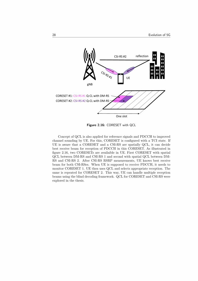
Figure 2.16: CORESET with QCL

Concept of QCL is also applied for reference signals and PDCCH to improvedchannel sounding by UE. For this, CORESET is configured with a TCI state. IfUE is aware that a CORESET and a CSI-RS are spatially QCL, it can decidebest receive beam for reception of PDCCH in this CORESET. As illustrated infigure 2.16, two CORESETs are availaible in UE. First CORESET with spatialQCL between DM-RS and CSI-RS 1 and second with spatial QCL between DM-RS and CSI-RS 2. After CSI-RS RSRP measurements, UE knows best receivebeam for both CSI-RSes. When UE is supposed to receive PDCCH, it needs tomonitor CORESET 1. UE then uses QCL and selects appropriate reception. Thesame is repeated for CORESET 2. This way, UE can handle multiple receptionbeams using the blind decoding framework. QCL for CORESET and CSI-RS wereexplored in the thesis.

Chapter3Current standards and proposed solution

This chapter explains the present standards and their implementation for beammanagement and channel sounding related to ABF. The working principles of cur-rent products are provided for the reader to get a better understanding of differentworking ways of beam management to make comparison with the proposed algo-rithms. Based on the problem description, proposed solutions have been stated forsolving the problem. Certain limitations existing with the current products havealso been mentioned.

3.1 Baseline solutions

As mentioned in the last chapter, P1, P2 and P3 processes are used for beammanagement in downlink which is the scope of the thesis. Being more precise,P2 measurement involving selection of best narrow beam among available narrowbeams is the area of exploration in this thesis. Channel measurement in the formof CSI-RS measurements are done and reported to the network. Best wide beamand narrow beam is selected based on RSRP values. Each wide beam consists ofa fixed number of narrow beams in ABF, 12 in our case. Beam switching takesplace from serving wide beam to new best wide beam and from serving narrowbeam to new best narrow beam.

Different baseline solutions for beam refinement in NR:

• Inter-narrowbeam selection: This process selects the best narrow beamamong the set of all narrow beams available based on the radio productin use. This is done by measuring and comparing RSRP values by UE.

• Inter-widebeam tracking: This is outer loop P2 process covered in Chapter2.

• Intra-widebeam selection: This is inner loop P2 process covered in Chapter2. This is carried in combination with outer loop P2 approach and is thefocus of the thesis.

• Two narrow beam selection: This process sweeps serving narrow beam andit’s two neighbouring narrow beams. In addition, inter wide beam selectiontracking mentioned above also repeats aperiodically. This algorithm reduces

29

30 Current standards and proposed solution

the number of narrow beam measurements and overhead greatly but is asub-standard solution as minimum narrow beam measurements are done.

• No narrow beam tracking: This is an extreme solution that does not performany measurements for best narrow beam selection and stays on the initialserving narrow beam. In addition, inter wide beam tracking mentionedabove also repeats aperiodically. This algorithm reduces the number ofnarrow beam measurements and overhead completely but is a sub-standardsolution as it relies only on wide beam tracking.

• Less narrow beam selection: This process sweeps serving narrow beam andit’s neighbouring narrow beams. No inter wide beam selection trackingmentioned above is done. This algorithm reduces the number of narrowbeam measurements and overhead but is a sub-standard solution as it doesnot involve wide beam tracking.

3.2 Proposed algorithms

Each narrow beam RSRP measurement consumes downlink resources for CSI-RStransmission and uplink resources for measurement reports which could otherwisebe used for data. CSI-RS overhead grows linearly with the number of connectedusers. This is a potential problem especially with more users like > 50.

• Increasing measurement period: Increasing the periodicity of triggering CSI-RS measurements to reduce overhead. It method does not require increasingnumber of trigger states.

• Minimize number of narrow beam measurements: Reducing the number ofCSI-RS symbols to measure is another proposed algorithm. This can betried without sacrificing a loss in beam management procedure of findingthe best beam. Based on radio product considered, overhead can be reducedto half by reducing the number of slots used for CSI-RS measurements tohalf.

Some limitations due to product hardware and specification standard applica-ble for beam management are stated below:

• Maximum trigger-states: The maximum number of aperiodic trigger statesis limited. The selection of the trigger states is done by MAC CE.

• Maximum number of CSI-RS beams to measure in a slot is limited to satisfyQCL.

• Performance: The implementation should be such that beam tracking per-formance is not sacrificed.

Chapter4Theoretical calculations

This chapter contains details about various parameters used for the thesis andresults from theoretical calculations. The results are provided for the reader to getbetter understanding of expected or ideal throughput values obtained on varyingperiodicity for channel estimation measurements and to make comparison with theresults from simulations using the proposed algorithms.

4.1 Transport Block Size (TBS)

Transport block is the payload for physical layer. It is mostly calculated for down-link, uplink or special sub-frame in TDD pattern. We have calculated TBS forshared channels PDSCH and PUSCH. The size of the transport block is calculatedusing several parameters. Successful reception of a downlink transmission dependson knowledge about various parameters. These are resource blocks, modulationscheme, transport block size and redundancy version. Information about some ofthese parameters is provided by 5-bit MCS field IMCS and the redundancy versionfield (rv) in the DCI to the UE. IMCS for NR is decided by UE based on threelook-up tables 5.1.3.1-1, 5.1.3.1-2 and 5.1.3.1-3 provided by 3GPP [2]. The ta-ble used depends on whether 256 Quadrature Amplitude Multiplexing (QAM) isconfigured or 64QAM is configured. LTE also uses these look-up tables to deter-mine MCS. It also tabulates transport block sizes with respect to MCS field. Thishelps in resource-block allocation. However, NR supports large range of transportblock sizes which are dynamic in nature. This is because of large bandwidthsused in NR. NR also supports different transmission duration and variations ofthe reference overhead signals. Hence, together they would result in many tablesrequired to cover all this which would also require modifications with changingparameters. Thus, a formula-based approach combined with a table for the small-est transport-block sizes is used in NR for flexibility. TBS is determined based onnumber of layers and PRB. It is determined separately for PDSCH and PUSCH.This formula is complex and is based on certain derived parameters that in turnare further based on certain derived parameters as shown in figure 4.1. These havebeen covered precisely in the sections below. For more detailed reading, readersare advised to refer to the specification document covering these calculations by3GPP [2].

31

32 Theoretical calculations

MCSTable

CalculateNumber

ofREs

Quantizer

Number of layers

MCS filed

Number of RBs

Transmission duration Number of REs

Code rate

Modulation order

Intermediate numberOf information bits

Transport Block Size

Figure 4.1: NR TBS calculation

TBS formula for PDSCH

Calculation of information about PDSCH

Ninfo = NRe · R ·Qm · v (4.1)

Different values in the equation 4.1 are as follows:

• Ninfo: Intermediate number of information bits, used for calculation of TBS.

• R: Target Code rate, which can extracted from table using MCS index.

• Qm: Modulation order, which can extracted from table using MCS index.

• v: Number of transmission layers

• NRe: Number of Resource Elements determined by UE

NRe is further defined as the following:

NRe = min(156,N′Re) · nPRB (4.2)


• nPRB: Total number of allocated PRBs for the UE.

• N′Re: Number of REs allocated for PDSCH within a PRB.

N′Reis further defined as the following:

N′Re = NRBSC ·N

symbsh ·NPRB

DMRS ·NPRBoh (4.3)


• NRBSC : 12 and is number of sub-carriers in a PRB

• Nsymbsh :This is the number of scheduled OFDM symbols of the PDSCH allo-

cation within the slot (maximum value as 12 or 14).

• NPRBDRMS:Number of REs for DM-RS per PRB in the scheduled duration in-

cluding the overhead of the DM-RS CDM groups without data.

Theoretical calculations 33

• NPRBoh : The overhead configured by a higher layer parameter in PDSCH

Serving Cell Configuration.

Upon calculation of Ninfo, value of TBS is determined using different cases.Overall structure has been mentioned below. However, covering all types of casesin detail is beyond the scope of the report.

• TBS for Ninfo ≤ 3824

N′info = max

[24, 2n ·

⌊Ninfo

2n

⌋](4.4)


• N′info = Quantized intermediate number of information bits

n = max(3, blog2(Ninfo)c − 6) (4.5)

Table 5.1.3.2-1 by 3GPP [2] is used to find the closest TBS that is not less thanN′info.

• TBS for Ninfo > 3824

N′info = max

[3840, 2n × round

[Ninfo − 24

2n

]](4.6)


• N′info: Quantized intermediate number of information bits

n = blog2(Ninfo − 24)c (4.7)

• round: The ties in the round function are broken towards the next largestinteger according to a very complex chain of algorithms mentioned in 3GPP[2].

TBS for PUSCH is calculated using series of more complex algorithms. Thethesis is focused on downlink throughput increment. TBS for uplink is beyond thescope of the thesis and we will limit our discussions to downlink.

4.2 Maximum throughput calculation

The approximate downlink and uplink data rates (Mbps) for a given number ofaggregated carriers in a band or band combination is computed in NR as follows[3]:

DR = 10−6 ·J∑

j=1

(v(j)Layers ·Q

(j)m · f(j)Rmax ·

NBW(j),µPRB · 12

Tµs· (1−OH(j))

)(4.8)

Different values of equation 4.8 are determined by different high-layer parameters.Readers are advised to go through specification sheet by 3GPP [2] for details.Functions of different values are as follows:


• J = Component carrier (CC) index

• v(j)Layers = Maximum number of supported transmission layers for uplink and

downlink

• Q(j)m = Maximum supported modulation order for uplink and downlink

• f(j) = Scaling factor which can take up values 1, 0.8, 0.75 and 0.4

• Rmax = 948/1024

• µ = Numerology [4]

• Tµs = Average OFDM symbol duration in a subframe for numerology. It iscalculated as 10−3

14.2µ assuming normal cyclic prefix

• NBW(j),µPRB = Maximum RB allocation in maximum supported UE bandwidth

BW(j) and numerology µ [5]. The term NBW(j),µPRB ·12

Tµscan also be written as

product of bandwidth BW(j) and spectral efficiency Sju

• OH = Overhead and takes values of 0.14 for frequency range FR1 for down-link, 0.18 for frequency range FR2 for downlink, 0.08 for frequency rangeFR1 for uplink and 0.10 for frequency range FR2 for uplink.

The above can also be summarized and calculated using TBS for EUTRA incase of MR-DC. Our implementation in NR high-band NSA is such a case whichuses MR-DC. The approximate data rate for a given number of aggregated carriersin a band or band combination is computed as follows [3]:

Data rate (Mbps) = 10−6 ·J∑

j=1

TBSj (4.9)

Different values of equation 4.9 are

• J: EUTRA CC index in MR-DC band combination

• TBSj: Total maximum number of downlink-SCH transport block bits re-ceived within a 1 ms Transmission time interval (TTI) for j-th CC [8]. Thisis based on the supported maximum MIMO layers for the j-th carrier byUE. It is also based on the modulation order and number of PRBs based onthe bandwidth of the j-th carrier.


4.3 Algorithm 1: Increasing periodicity of CSI-RS

Following section describes the calculation of throughput with varying P2 period-icity:

4.3.1 Various parameters used:

• TDD: Pattern 4+1

• SSB periodicity: Fixed for current products

• Number of connected UEs: Varied with values of 1, 5, 10, 20, 50 and 100

• P2 CSI-RS period per active UE: Varied with values of 20 ms, 40ms, 80ms,160ms, 320ms and 640ms

• Slots: PUSCH and PDSCH slots available in the TDD 4+1 pattern arecounted containing symbols with CSI-RS for P2 and LA, PUCCH and gap

• Bandwidth of operation: 100 MHz

• CC: Throughput is calculated per CC (J = 1 in (4.9))

• DM-RS: TBS is calculated for 1 DM-RS

• TBS: Different TBS pertaining to PDSCH and PUSCH slots are calculatedusing equations (4.1)-(4.7)

• Block Error Rate (BLER): It defined as ratio of the number of erroneoustransmissions to the total number of transmissions. The outputs are multi-plied with a factor of 2× 10−2 is used to account for re-transmissions.

4.3.2 Theoretical results

Equation (4.9) is used to calculate the maximum data rate for downlink. Theobtained data rates are tabulated below. When number of users is 100, the valuefor throughput for baseline periodicity of 40 ms is negative. This means that allTDD slots will be consumed for channel sounding and no resources will be left fordata. Decreasing periodicity below baseline to 20 ms has a negative impact ondata rates and the effect is more profound when the number of users become 50and more.

The results show that increasing periodicity of CSI-RS for a fixed numberof users increases overall system throughput. The results also show decrease inthroughput with increase in users. This is intuitive as more resources are usedfor channel measurements with increase in number of users. But even with moreusers, increasing periodicity has as positive effect on throughput indicating thatthis algorithm is effective for P2 process. In fact, the increase is 0.88% for 1 userwhile it goes up to 95.81% for 50 users when compared to baseline. We will verifythe same in simulations and make comparisons.


Users = 1 Users = 5Periodicity Throughput

20 526.840 531.880 534.8160 535.5320 536.2640 536.5

Periodicity Throughput20 483.340 508.480 521.0160 527.2320 530.4640 532.0


20 429.040 479.280 504.3160 516.9320 523.1640 526.3

Periodicity Throughput20 320.440 420.880 471.0160 496.1320 508.7640 514.9


20 -5.440 245.680 371.1160 433.8320 465.2640 480.9

Periodicity Throughput20 -276.940 99.680 287.8160 381.9320 429.0640 452.5

Users = 100Periodicity Throughput

20 -584.440 -46.480 204.6160 330.1320 392.8640 424.2

Table 4.1: Throughput (Mbps) by varying P2 periodicity (ms) fordifferent number of users*

*Negative data rates indicate all TDD slots consumed for channelsounding and no resources left for data.


4.4 Algorithm 2: Decreasing CSI-RS measurements

The following section describes the calculation of expected gain when reducing 12beams to 6 beams:

4.4.1 Various parameters used:

• TDD: Pattern 4+1

• Periodicity for measurements: 20 ms or 160 slots

• maximum number of P2 occasions in 20 ms: Defined as 32 as mentioned inCSI-RS architecture sub-section but is limited currently to 27. We assumethis upper bound is hit due to lot of inactive UE

• Slots: PUSCH and PDSCH slots available in the TDD 4+1 pattern arecounted containing symbols with CSI-RS for P2 and LA, PUCCH and gap

• Bandwidth of operation: 100 MHz

• CC: Throughput is calculated per CC (J = 1 in (4.9))

• DM-RS: TBS is calculated for 1 DM-RS

4.4.2 Theoretical results

First, calculation of total number of PDSCH symbols was done. With 12-beamCSI-RS, 12*27 PDSCH symbols are consumed for channel sounding and remainingare left for data. Calculating the same with proposed algorithm of 6 beams de-creases to 6*27. Thus, overall increase in downlink resources with new algorithm is13.73%. In general, every OFDM symbol saved leads to gain in 2.29% in downlinkresources. We will verify the same with simulations.

Chapter5Methodology

This chapter contains details of simulation environment, different parameters used,various use cases and the process followed to obtain results in an Ericsson simula-tor.

5.1 Proposed algorithms

Two different solutions are proposed to mitigate the problem of overhead in P2beam management procedure. These have been discussed in an earlier chapter indetail. These are as follows:

• Increasing measurement period of P2 process

• Minimizing number of narrow beam measurements of P2 process

5.2 Simulator overview

This section gives an overall picture of the simulation environment used for testingthe effectiveness of the proposed algorithms. A very powerful simulator developedinternally by Ericsson has been used for the thesis. It provides ideal state of theart 5G NR environment and supports multiple 5G features. Especially, beam-forming and beam management procedures mimicking the current products areprovided in the simulator which were very helpful in the thesis. Iterating a cer-tain parameter of interest over many values was also facilitated by the simulator.A simulation seed encompasses all possible random configurations of parametersrelated to the simulation. Randomness of the seed influence the surroundings inwhich the solutions are tested. Thus, simulations which are run with multipleseeds add credibility to the results as in the case of the thesis. In addition toiterating the simulations over multiple seeds, they were also iterated over multiplesimulations. Thus, results obtained from multiple seeds as well as multiple simula-tions strengthened their trustworthiness. The simulations were run with existingbaseline algorithm of beam management and also with proposed solutions for com-parison. These were run on powerful servers provided by Ericsson minimizing theprocessing time. The simulator has several interfaces to run simulation on. Twosuch user interfaces were used to run simulations as follows:

39

40 Methodology

Main user interface

It is the central user interface available to run simulations. It gives the func-tionality of choosing the simulator file along with associated log file defined withparameters for which results are to be stored. Thus, multiple jobs can be sub-mitted simultaneously using this interface. One job refers to running a simulationwith one specific set of parameters. Hence, instead of changing the parametersevery time after a successful simulation, this interface helps a user define all iter-ations in the simulator file and then submit the file for a run. Numerous outputlog files were generated by the simulator storing various results from different usecases. It also generates multiple MATLAB files associated with various seeds andsimulations storing results which are post-processed later. This was the primaryinterface for running simulations and storing results.

Graphical user interface

As the name suggests, it is the visual graphical user interface available to runsimulations. It also gives the functionality of choosing the simulator file. However,unlike main interface, multiple jobs can not be submitted together in this interface.One specific set of parameters are run each time and are changed every timeafter a successful simulation. The interface has several user window planes toconfigure parameters and view results. It has a simulator setup plane windowshowing all possible set of parameters to change. It also has a logging window tochoose different log values such as Cell downlink (DL) throughput, File transferProtocol (FTP) throughput, RSRP values and so on. When a simulation runbegins, different logs can be viewed in the result window console. Also, theseresults can be viewed as plots in charts console. It also gives the functionality ofsaving the changes made here in new simulator files. This was also heavily usedalong with main interface to visualize different logs and see the results in plots.

5.3 Traffic models

Three different traffic models have been explored in the simulator. These modelshave been curtailed to match real time data traffic. For achieving better results,real time data collected from three operators from different parts of the world atdifferent times has been used. Distribution of downloaded user data, uploadeduser data and session length assuming an RRC inactivity time of 10s was used tofine-tune the models.

Full buffer traffic model

This model is close to the ideal situation where the traffic has full buffer. Thecell always serves certain number of UE and the packets are always availablewith gNB to send to connected UE. So at every TTI, there is data to transmit.On successful download of a package, a new package is always generated. Thedeployment is interference limited. UEs always keep downloading files and thegNB is always transmitting. This model can be assumed to be like User Datagram

Methodology 41

Protocol (UDP) which is suitable for cases where error checking and correction isnot done and overhead from such processing is avoided. In this model, we have afixed number of UE always connected to the system. In case a UE dies out due toinactivity, a new UE is instantly created thus maintaining the overall head-count.This model was to have a complete understanding of the system behaviour changeon implementing the proposed algorithms.

FTP traffic model

This bursty model involves small, medium and large files of upto 100 MB sizebeing downloaded by all UE. The download is requested by the UE. The gNBbuffer gets exhausted after successful download and UE need to wait for a certaintime before next arrival. The packets for download also arrive at a fixed pre-defined arrival rate. This model can be assumed to be like Transmission ControlProtocol (TCP) where active open, re-transmission and error-detection is done.This adds to reliability to network. In this model, we have a fixed number ofUEs always connected to the system as for full buffer model. This deployment isalso interference limited. The simulations also include incomplete sessions such asthose for cell-edge UEs. Excluding such sessions could skew statistics. This typeof model is used dominantly for web applications.

Realistic FTP traffic model

This traffic model is a variation of FTP model and more close to the real lifescenario. Unlike the other two models, we do not have fixed number of UEsalways connected to the system. Number of active UE depend on a factor calledintensity. For example, if intensity = 1, we have 1 user generated per second.If the simulation runs for 10 simulation seconds, we will have a total of 10 UE.However, not all of them will be active or connected at all times. Hence, numberof generated users is a function of time. The final results are a combination of thetwo FTP models.

5.4 Key Performance Index

To investigate reliability of obtained results from proposed algorithms and com-paring them with existing baseline algorithm, Key Performance Index (KPI) wasselected. Various parameters such as Bit Error rate (BER) and RSRP values wereconsidered. Finally, best KPI found for the thesis was overall system throughput.However, other parameters not considered as KPI were also studied to increasethe understanding of the simulation environment. Two types of throughput usedfor running simulations are described as following:

Cell throughput

This kind of throughput in the simulator gives the instantaneous value of through-put generated every specified time interval. Typically, the time interval is verysimulation second but can be customized to occur more or less frequently. The

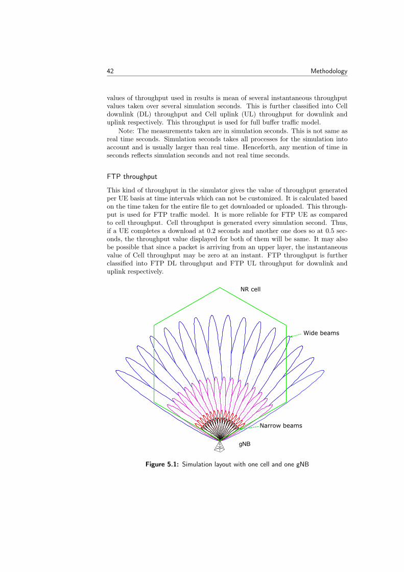
42 Methodology

values of throughput used in results is mean of several instantaneous throughputvalues taken over several simulation seconds. This is further classified into Celldownlink (DL) throughput and Cell uplink (UL) throughput for downlink anduplink respectively. This throughput is used for full buffer traffic model.

Note: The measurements taken are in simulation seconds. This is not same asreal time seconds. Simulation seconds takes all processes for the simulation intoaccount and is usually larger than real time. Henceforth, any mention of time inseconds reflects simulation seconds and not real time seconds.

FTP throughput

This kind of throughput in the simulator gives the value of throughput generatedper UE basis at time intervals which can not be customized. It is calculated basedon the time taken for the entire file to get downloaded or uploaded. This through-put is used for FTP traffic model. It is more reliable for FTP UE as comparedto cell throughput. Cell throughput is generated every simulation second. Thus,if a UE completes a download at 0.2 seconds and another one does so at 0.5 sec-onds, the throughput value displayed for both of them will be same. It may alsobe possible that since a packet is arriving from an upper layer, the instantaneousvalue of Cell throughput may be zero at an instant. FTP throughput is furtherclassified into FTP DL throughput and FTP UL throughput for downlink anduplink respectively.

gNB

NR cell

Wide beams

Narrow beams

Figure 5.1: Simulation layout with one cell and one gNB

Methodology 43

5.5 Simulator parameters

Various parameters used for running simulations are as follows:

• Simulation time: Variations of 5s, 10s and 20s

• Seeds: Combinations of 10, 25, 50 and 100

• Carrier bandwidth: 100 MHz with

• Resource block: 66 PRBs and 8 CCE CORESET Aggregation 8 [4]

• Carrier frequency: 39 GHz high-band

• Deployment scenario: 1 gNB with 1 cell as shown in figure 5.1

• Cell radius: 100 m as shown in figure 5.2

• Numerology: µ=3 (120 KHz OFDM sub-carrier spacing)

• Processing speed: 8000 slots/second corresponding to µ=3.

• TDD pattern: 4+1

• Radio link: Multi-path slow fading multi-user propagation model with Ad-ditive White Gaussian noise (AWGN) was used. This design is based onExtended Pedestrian A model (EPA) [10]

• Periodicity of CSI-RS: Different periodicity values were used to see effect onthroughput values. However, the simulator is not designed take variations ofperiodicity. Instead, it counted variations in term of TDD slots used for CSI-RS measurements. Therefore, variations of slots amounting to variations ofperiodicity was used. Variation used were 160, 320, 640, 1280, 2560 and5120 slots reflecting 20 ms, 40 ms, 80 ms, 160 ms, 320 ms and 640 ms inperiodicity respectively. Henceforth, we will refer to periodicity in ms forease of representation and discussion.

• Re-transmissions: Maximum number of H-ARQDL and UL re-transmissionswas set to 7

• Antenna deployment:

– Type: MACRO MU-MIMO using muti-port antenna mapping

– Dimensions: Length 0.5 m and width 0.5 m [9].

– Height: 23 m in accordance with urban macro cell (3D-UMa) withhigh UE density [9].

– Antenna tilt: Measured by zenith angle and set to 14◦. Antenna zenithangle in the simulator is defined as antenna tilt towards the groundand applies to both narrow and wide beams. Thus, an angle tilt ofzero degrees reflects horizontal antenna.

– Antenna elements: 128 antenna elements divided in 8 rows were used.Antenna elements are individual antennas used to beamform the sig-nal.

44 Methodology

– Antenna ports: 2 transceiver ports per antenna which also function asCSI-RS ports

– Sector: Geographical sector of width 120 m and height 30 m

– Wide beams:

∗ Horizontal wide beams: 3∗ Vertical wide beams: 4

– Narrow beams:

∗ Horizontal narrow beams: 34∗ Vertical narrow beams: 4

• UE:

– Number of UE:

∗ Fixed UE numbers: 1, 5, 10, 20, 30, 40, 50, 75, 100∗ Intensity: 0.5, 1, 5, 10, 20

– Height: 1.5 m

– UE antenna elements: 2 elements per UE with 2 transceiver ports

– UE speed: Different UE speeds were used to test the effect of the algo-rithms proposed. The simulator is designed to take measurements inmeter per second (m/s). The values used were 0, 1.38, 2.78, 13.89 and27.78 m/s reflecting 0, 5, 10, 50 and 100 kilometer per hour (km/hr).Henceforth, we will refer to speeds in km/hr for ease of representationand discussion.

– UE power class: Class 3 of maximum cell downlink power 23 dBm(with tolerance of ±2) for non-CA configuration and maximum uplinkpower of 0.25 dBm was used [5]

– Inactivity timing: UE was supposed to be inactive if it did not transmitor receive anything for 10s or more.

– UE types:· DL FTP UE: single file transfers for download· UL UE: continuous file transfer for upload· Short UE: single transmission· Chatty UE: chatty trafficOverall number of UE is divided in these 4 types based ondata collected from 3 different operators. Chatty and ShortUE are used for impact of background light traffic, whichrepresent the majority of RRC sessions.

– Movement direction:· Straight mover UE· Origination of UE at any position in the cell is determinedby the randomness of the simulation seed· Continues to move until the end of the simulation

Methodology 45

· Moves straight in any direction until they reach a circle thatcircumscribes the hexagonal simulation area· Hereafter, bounce back and continue straight movement in anew direction as shown in figure 5.2.

(0,0) (100,0)(-100,0)

(0,100)

(0,-100)

(UE)

gNB

Figure 5.2: Straight mover

5.6 Simulation procedure

In the simulation procedure, UEs are generated according to environment patternin a hexagonal cell belonging to a gNB. The distance between hexagon’s centre toits six corners is 100 m and is called radius of the cell. The BS along with widebeams containing narrow beams has been shown in figure 5.2. Beamforming isdone in MU-MIMO layers and beams overlap each other as shown in the figure5.1. UE tries to establish a connection with the BS through initial access by beamsweeping over SSBs transmitted using P1 process. This results in connection ofUE to best wide beam by measuring RSRP values. After P1, UE establishesitself with the best narrow beam of wide beam by P2 process. The beam trackingalgorithm ensures stationary or moving UE is always connected to the best narrowbeam by measuring and comparing RSRP values through CSI-RS measurements.Different RSRP values for serving beam measurements were recorded to look atthe effectiveness of the algorithms. The periodicity of L1 SSB RSRP measurementand CSI-RS RSRP measurement was aligned to be same at 20 ms. To reduce thisoverhead, two proposals are mentioned. These were simulated as follows:

46 Methodology

5.6.1 Algorithm 1: Increasing periodicity of CSI-RS

CSI-RS measurement periodicity at baseline was simulated and then varied for allcombinations mentioned in section 5.5. Further, the speed of UE was also variedfor all combinations mentioned in section 5.5. These simulations were furtherclassified in the three traffic models:

• Full buffer: For idealistic full buffer model, the number of UE was varied as1, 5, 10, 20, 50 and 100. Cell DL and UL throughput was recorded in logfiles.

• FTP model: For FTP model, the number of UE was varied as 1, 5, 10, 20,50, 75 and 100. FTP DL and UL throughput was recorded in log files.

• Realistic FTP model: For realistic FTP model, the number of UE wasvaried using intensity parameter as mentioned in section 5.5. FTP DL andUL throughput was recorded in log files.

5.6.2 Algorithm 2: Decreasing CSI-RS measurements

12 narrow beams exists in a wide beam. CSI-RS measurements take place for all 12narrow beams in the serving wide beam. This was already simulated in algorithm1 and then changed to 6 beams in this algorithm. The periodicity for CSI-RS wasset to baseline. Further, the speed of the UEs was also varied for all combinationsmentioned in section 5.5. Single periodicity was used for these simulations. Thesesimulations were further classified in two traffic models:

• Full buffer: For idealistic full buffer model, the number of UEs was variedas 5, 10, 20, 30, 40, 50, 75 and 100. No simulation was run for a single UEas it would not be enough to gain reliability of this solution. The numberof combinations of UE tested was also increased to understand system be-haviour in a better way. Cell DL throughput and cell UL throughput wererecorded in log files.

• FTP model: For FTP model, the number of UE was varied similar to fullbuffer model. FTP DL throughput and FTP UL throughput were recordedin log files. No simulations were run for realistic FTP model as that modeldoes not have fixed number of users and would not suit this algorithm.

Chapter6Results

This chapter presents output of the algorithm behaviour in different scenarios.The results are also compared to theoretical outputs and baseline solutions.

6.1 Theoretical result for periodicity increase

Figure 6.1 shows the theoretical results for different number of stationary users.This is also represented with absolute values in table 4.1. The results show increas-ing periodicity has as positive effect on DL throughput at 0 km/hr. Also, thereis decrease in throughput with increase in users. However decreasing periodicitybelow baseline to 20 ms case has a negative impact on data rates especially withincrease in number of users beyond 50. Similarly, values less than 20 ms werealso tried and the results were found to be even worse. Those results have beenexcluded from the report.

1 5 10 20 50 75 100

Number of users

-600

-400

-200

0

200

400

600

Dow

nlin

k th

roug

hput

(M

bps)

Periodicity = 20 ms

Periodicity = 40 ms

Periodicity = 80 ms

Periodicity = 160 ms



Figure 6.1: Theoretical DL throughput varying P2 periodicity. Neg-ative values show all resources consumed for channel sounding.

47

48 Results

6.2 Algorithm 1: Increasing periodicity of CSI-RS

6.2.1 Traffic Model: Full buffer

1 5 10 20 50 75 100

Number of users

200

250

300

350

400

450

500

550

600

Dow

nlin

k th

roug

hput

(M

bps)

Periodicity = 40 msPeriodicity = 80 msPeriodicity = 160 msPeriodicity = 320 msPeriodicity = 640 ms

Figure 6.2: Average Cell DL throughput with varying P2 periodicity(5km/hr)

Figure 6.2 shows the DL throughput for different number of pedestrian usersat 5km/hr. When compared to figure 6.1, we find that the behaviour is similarwith better data rates with increase in periodicity. However, comparing absolutevalues shows that the result is full buffer is mostly lower than theoretical casebut sometimes higher, especially with less users. This can be due to the fact thatinterference comes into play in simulator which is absent while making theoreticalcalculations. Also, higher throughput may be present for full buffer than theo-retical due to effect of multi-path adding constructively thus giving better datarates.

Figure 6.3 shows behaviour of periodicity change at speed of 50km/hr. Here,we again find that effect of periodicity change is better for all number of users.

Similarly, results for all other use cases have been included in the Addendumsection for readers to have a complete idea of system behaviour. In full buffermodel, cell DL throughput increases with the increase in periodicity. Overall datarates decrease as the number of users increase. However, the gain is less whennumber of UE increases beyond 50. Also, the effect of increasing periodicity ismore profound when the speed of UE increases.

Results 49

1 5 10 20 50 75 100

Number of users

150

200

250

300

350

400

450

500

Dow

nlin

k th

roug

hput

(M

bps)


Figure 6.3: Average Cell DL throughput with varying P2 periodicity(50km/hr)

6.2.2 Traffic Model: FTP

Figure 6.4 shows the results for different number of pedestrian users at 5km/hr.It can be seen that increasing periodicity has positive effect on rise in FTP DLthroughput. Decreasing periodicity to 20 ms is found to be a bad choice as thethroughput values fall drastically as was seen in theoretical results too.

Figure 6.5 shows results for different number of high-speed users at 100km/hr.An example of such a case in reality can be when travelling on a train where manyusers may be connected to a single cell from a single gNB. It can be seen thatincreasing periodicity has positive effect on rise in FTP DL throughput for allusers.

Similarly, results for all other use cases have been included in the Addendumsection for readers to have a complete idea of system behaviour. In FTP buffermodel, FTP DL throughput increases with the increase in periodicity. Overalldata rates decrease as the number of users increase. Unlike full buffer model, thegain is good even when number of UE increases beyond 50.

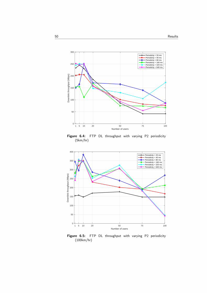
50 Results

1 5 10 20 50 75 100

Number of users

0

50

100

150

200

250

300

Dow

nlin

k th

roug

hput

(M

bps)

Periodicity = 20 msPeriodicity = 40 msPeriodicity = 80 msPeriodicity = 160 msPeriodicity = 320 msPeriodicity = 640 ms

Figure 6.4: FTP DL throughput with varying P2 periodicity(5km/hr)

1 5 10 20 50 75 100

Number of users

0

50

100

150

200

250

300

350

400

Dow

nlin

k th

roug

hput

(M

bps)


Figure 6.5: FTP DL throughput with varying P2 periodicity(100km/hr)

Results 51

6.2.3 Conclusion

Using results from FTP and full buffer model, it can be clearly seen that increas-ing periodicity has a positive effect on data rates. Decreasing periodicity belowbaseline was not found to be a good approach. For full buffer model, that gainin throughput is more for users less than 50 while it is good for all user cases inFTP model. This may be because of the fact that FTP model is more realisticthan full buffer. Also, the effect of increasing periodicity is more profound whenthe speed of UE increases. Sometimes, the system throughput behaves abruptlyas can be seen in the Addendum section. This may be due to the fact that FTPthroughput accounts for file transfers which may be effected by some higher-layereffects. Relying on absolute results may be harmful and thus focus is based on thelarger picture of overall system behaviour. Since real time traffic is more close toFTP, we can conclude that this algorithm is good for decreasing CSI-RS overhead.

The simulator shows good results in most use cases for even very high peri-odicity values like 640 ms. This may not translate into reality and UE may startdropping out due to less channel sounding. The simulator takes interference aswell as fading into consideration. However, since the simulation is limited to onecell, most of the communication between UE and gNB is via Line of Sight (LOS).For Non-Line of Sight (NLOS) propagation in fading dips, increasing periodicityto a very large value may be harmful. This hypothesis can only be verified whenthe algorithm is put to practice in real-time measurements which could not bedone for the thesis. Overall, with more than 50 UE, 80 ms and 160 ms are foundto be good choices for periodicity.

52 Results

6.3 Algorithm 2: Decreasing CSI-RS measurements

6.3.1 Traffic Model: Full buffer

5 10 20 30 40 50 75 100

Number of users

100

150

200

250

300

350

400

450

500D

ownl

ink

thro

ughp

ut (

Mbp

s)

6 beams @ 0 km/hr6 beams @ 5 km/hr6 beams @ 10 km/hr6 beams @ 50 km/hr6 beams @ 100 km/hr12 beams @ 0 km/hr12 beams @ 5 km/hr12 beams @ 10 km/hr12 beams @ 50 km/hr12 beams @ 100 km/hr

Figure 6.6: Cell DL throughput comparison between 6 beams and12 beams with varying speed

Figure 6.6 shows comparison between cell DL throughput values for 6 beamsand 12 beams CSI-RS measurements for different UE speed in full buffer model.The periodicity has been fixed to baseline. As seen, the downlink throughput gainis visible for 6 beams when compared to 12 beams. There is an exception of speed= 100km/hr where degradation occurs for some number of users. This may bedue to the high speed of users which might be unfavourable for migration from12 to 6 beams. Also, the gain % achieved is approx 9-25 % which is in range astheoretical calculation if 13.73 % (Chapter 7, section 4.5) and even more. Therise in downlink gain can be explained from the fact that theoretical gain wascalculated based on an assumption that maximum UE is inactive leading to upperbound on maximum CSI-RS measurements of 27 being achieved. This leads tomore data PDSCH slots being used for CSI-RS instead. This upper bound maynot always be true which can result in higher downlink gain as in these cases. Thesame can be seen in figure 6.7. Based on full buffer model, this algorithm seemsto produce good results.

Results 53

5 10 20 30 40 50 75 100

Number of users

0

5

10

15

20

25

30

Gai

n (%

)

Average Cell DL throughputAverage Cell UL throughput

Figure 6.7: Cell DL and UL throughput gain (5km/hr)

6.3.2 Traffic Model: FTP

Figure 6.8 shows comparison between FTP DL throughput values for 6 beams and12 beams CSI-RS measurements for different UE speed in FTP model. As seen,the throughput gain is visible for some cases of 6 beams when compared to 12beams. However, for some cases, decrease in throughput is observed. For few highspeed cases, no FTP DL throughput values were obtained. Even in case of thegain, only 2.3 % approx is achieved which is way less than expected theoreticalcalculation of 13.37% as in section 4.5 and as obtained for full buffer model. Thesame can be seen in figure 6.10. To understand this difference, uplink throughputwas investigated.

Figure 6.9 shows comparison between FTP UL throughput values for 6 beamsand 12 beams CSI-RS measurements for different UE speed in FTP model. Asseen, the throughput gain is visible for 6 beams when compared to 12 beams forsome cases. However, for most cases, decrease in throughput is observed especiallyfor high speed UE. Gain % achieved can be seen in figure 6.10.

54 Results

5 10 20 30 40 50 75 100

Number of users

0

100

200

300

400

500

600

Dow

nlin

k th

roug

hput

(M

bps)

6 beams @ 0 km/hr

6 beams @ 5 km/hr

6 beams @ 10 km/hr

6 beams @ 50 km/hr

6 beams @ 100 km/hr

12 beams @ 0 km/hr

12 beams @ 5 km/hr

12 beams @ 10 km/hr

12 beams @ 50 km/hr

12 beams @ 100 km/hr

Figure 6.8: FTP DL throughput comparison between 6 beams and12 beams with varying speed

5 10 20 30 40 50 75 100

Number of users

0

5

10

15

Upl

ink

thro

ughp

ut (

Mbp

s)

6 beams @ 0 km/hr6 beams @ 5 km/hr6 beams @ 10 km/hr6 beams @ 50 km/hr6 beams @ 100 km/hr12 beams @ 0 km/hr12 beams @ 5 km/hr12 beams @ 10 km/hr12 beams @ 50 km/hr12 beams @ 100 km/hr

Figure 6.9: FTP UL throughput comparison between 6 beams and12 beams with varying speed

Results 55

5 10 20 30 40 50 75 100

Number of users

-3

-2

-1

0

1

2

3

4

5

Gai

n (%

)

FTP DL throughputFTP UL throughput

Figure 6.10: FTP DL and UL throughput gain (5km/hr)

56 Results

6.3.3 Conclusion

Using results from full buffer model, it can be seen that decreasing number of CSI-RS measurements has a positive effect on data rates. However, FTP traffic modelshows that this algorithm has little gain of DL data rates. The reason for this isdegradation UL throughput. As UL data rates go down, TCP acknowledgementsthat are needed for DL transmissions become very slow. Congestion control isanother feature used by TCP to avoid congestive collapse. This is performedusing congestion window which limits total number of unacknowledged packetsthat might be in transit completely. This causes DL incoming rate from higherlayers to go down. This is the reason for some cases where no FTP DL throughputis obtained in simulations. In these cases, only FTP UL throughput is obtained.The effect is more profound when speed of UE increases. As mentioned in previouschapter, FTP throughput is generated on per UE basis. Since UE is typecast in DLand UL before simulation run, no FTP DL throughput being generated indicatesthat DL UE is unable to download data and becomes inactive due to RRC sessiontime-out and only UL UE is active. On an overall, there is decrease in the numberof FTP DL throughput occasions for 6 beams when compared to same run with12 beams. For the present simulated environment, UL is throttled and becomes abottleneck which then effects DL data rates. Little overhead saving for DL doesnot lead to large expected gain while system degrades when shifting from 12 beamsto 6 beams. Although algorithm 2 has been explored for P2 inner-loop narrow-beam refinement in the simulator, the same can also be extended to P2 outer-loopwide-beam refinement. Using 6 beams instead of 12 for both loops in P2 processis unhealthy.

Although gain exists for full buffer model, real time traffic is more like TCPor QUIC than UDP. Therefore, we conclude that this algorithm is not suitablefor decreasing overhead of CSI-RS measurements. Some measures can be taken toamend this behaviour which has been covered in the next chapter.

The results obtained and the conclusion are under specific parameters of thesimulated environment. They may or may not translate similarly in real-time runsor other simulated environments.

Chapter7Future Scope

This chapter contemplates obtained results and provides thoughts on extension ofbeam-management in future.

7.1 Summary

Reliability of simulated throughput is difficult to testify. Data rates vary a lotdepending on number of users, type of users, traffic model, multi-path environmentetc. Care was taken to have an array of use cases and models in close relation toreal-time data to provide reliability to obtained results.

Looking in retrospection, algorithm 1 of increasing P2 periodicity of CSI-RSmeasurements was found to be a good idea for saving resources. This algorithm iseasy to implement in baseline without making lot of changes in existing productcode. Also, the number of aperiodic trigger states for P2 does not increase in thisprocess. Considerable gain in data rates was observed which can be verified fromvarious plots in Chapter 6 and the Addendum section.

Algorithm 2 of decreasing P2 CSI-RS beam measurements on the other handwas not found to be a good idea for saving resources in the simulations. Thisalgorithm was relatively more complex in implementation. The gain in throughputfor downlink is negligible if any. Uplink was found to be the prime tailback.

But as George E.P.Box quoted "All models are wrong, but some are useful",key takeaway from algorithm 2 is that more focus in today’s communication stan-dards is made on downlink. It is the biggest demand of the market and userdownlink speed always takes the center stage. However, this should not lead toovershadowing of uplink. In order for downlink to work effectively, uplink needs tobe managed properly. Algorithm 2 could work well if some new balanced duplexpattern is used in future with more focus on uplink and increase in uplink slots likeTDD 4+2. Another way to amend this problem could be to implement MachineLearning (ML) algorithm which might record/predict correlated measurementsand then decrease number of beams for measurements. Having said that, radiopropagation environment is highly volatile and the reliability of such algorithmmay be less.

57

58 Future Scope

7.2 Future work

As mentioned in Chapter 4, various processes of beam management exists andexploring all was beyond the scope of the thesis due to limitations of time. Suchcases may be potentially exploited of the future have been stated in this section.

P1 process of initial beam establishment and P3 process of UE side beamsweeping constitute very important part of beam management which could havesimilar aspects to explore.

The thesis was implemented in Ericsson’s internal simulator. Analysing andpredicting real-time output and behaviour of the algorithms still remains unex-plored and could present challenges that may lead to further studies.

Also, the simulations are run for one cell with one BS. The scenario of han-dovers between multiple BSs can be investigated.

One beam management feature is LA measurement which happens on theserving narrow beam twice as often as P2 measurement. A lot of research ison-going in this process and could be possibly explored in future too.

A PDSCH slot containing CSI-RS resources for P2 measurement cannot beused for anything else in current product for simplicity. However, there is on-going work to remove this limitation. This could be a very good area to work andexplore.

Extended Kalman Filter (EKF) is an area of gaining popularity, especiallyfor mmWave beam tracking. It has also been applied in new trends of vehicu-lar communication beam tracking for more frequent channel estimations due touse of narrow beams [43]. Vehicular communication is more challenging, particu-larly because of fast-changing environments. The same could be applied to beammanagement process leading to better results.

Finally, Machine Learning (ML) is an area of fast growth. It could also beexplored for beam management

References

[1] 3rd Generation Partnership Project (3GPP), "Study on New Radio (NR)access technology (Release 15)", 3GPP TR 38.912 V15.0.0, Technical Speci-fication, 2018.

[2] 3rd Generation Partnership Project (3GPP), "Study on New Radio (NR)access technology - Physical layer procedures for data (Release 15)", 3GPPTS 38.214 version 15.3.0, Technical Specification, 10-2018.

[3] 3rd Generation Partnership Project (3GPP), "Study on New Radio (NR)access technology - User Equipment (UE) radio access capabilities (Release15)", 3GPP TS 38.306 version 15.5.0, Technical Specification, 05-2019.

[4] 3rd Generation Partnership Project (3GPP), "Study on New Radio (NR)access technology - Physical channels and modulation" (Release 15)", 3GPPTS 38.211 version 15.2.0, Technical Specification, 07-2018.

[5] 3rd Generation Partnership Project (3GPP), "Study on New Radio (NR)access technology - User Equipment (UE) radio transmission and reception"(Release 15)", 3GPP TS 38.101 version 15.3.0, Technical Specification, 2018.

[6] 3rd Generation Partnership Project (3GPP), “Study on New Radio (NR)Access Technology - Physical Layer Aspects (Release 14)”, 3GPP TR 38.802,2017.

[7] 3rd Generation Partnership Project (3GPP), “Study on New Radio (NR)Access Technology - Medium Access Control (MAC) protocol specification(Release 15)”, 3GPP TR 38.321, 2018.

[8] 3rd Generation Partnership Project (3GPP), "Study on New Radio (NR)access technology - Evolved Universal Terrestrial Radio Access (E-UTRA);Physical layer procedures " (Release 13)", 3GPP TS 36.213 version 13.2.0,Technical Specification, 08-2016.

[9] 3rd Generation Partnership Project (3GPP), "Study on 3D channel model forLTE" (Release 12)", 3GPP TR 36.873 version 1.0.0, Technical Specification,09-2013.

59

60 References

[10] 3rd Generation Partnership Project (3GPP), "Study on LTE - Evolved Uni-versal Terrestrial Radio Access (E-UTRA); Base Station (BS) conformancetesting" (Release 10),TS 36.141 version 10.8.0 , Technical Specification, 09-2013.

[11] 3rd Generation Partnership Project (3GPP), "Study on LTE - Evolved Uni-versal Terrestrial Radio Access (E-UTRA); Physical layer procedures" (Re-lease 10), TS 36.213 version 10.4.0 , Technical Specification, 01-2012.

[12] I. Da Silva et al., “Tight Integration of New 5G Air Interface and LTE toFulfill 5G Requirements,” 2015 IEEE 81st Vehicular Technology Conference(VTC Spring), Glasgow, 2015

[13] 3GPP TS 37.340 v15.0.0, 3rd Generation Partnership Project; NR; Tech-nical Specification Group Radio Access Network; Multi-connectivity;Overalldescription; Stage-2 (Release 15), January 2018

[14] ITU-R, IMT Vision – Framework and overall objectives of the futuredevelopment of IMT for 2020 and beyond Recommendation M.2083-0, September 2015. URL http://www.itu.int/en/ITU-R/study-groups/rsg5/rwp5d/imt-2020/Pages/default.aspx

[15] 3rd Generation Partnership Project (3GPP), “Beam Management study forNew Radio (NR) Access Technology”, 3GPP TR 38.802, 6.1.6.1, 2017.

[16] 3rd Generation Partnership Project (3GPP), “Radio Resource Control (RRC)Protocol specification for New Radio (NR) Access Technology”, 3GPP TR38.331, 2018.

[17] 3rd Generation Partnership Project (3GPP), “Study on test methods for NewRadio (NR) Access Technology”, 3GPP TR 38.810, 09-2018

[18] 3rd Generation Partnership Project (3GPP); "Group Radio Access Network;Study on Scenarios and Requirements for Next Generation Access Technolo-gies"; 3GPP TR 38.913 v14.3.0, (Release 14),August 2017

[19] 3rd Generation Partnership Project (3GPP), “Study on Non-Orthogonal Mul-tiple Access (NOMA) for NR”, 3GPP TR 38.812, 2017

[20] Wonil Roh ; Ji-Yun Seol ; Jeongho Park ; Byunghwan Lee ; Jaekon Lee; Yungsoo Kim ; Jaeweon Cho ; Kyungwhoon Cheun ; Farshid Aryanfar,“Millimeter-wave beam forming as an enabling technology for 5G cellularcommunications: theoretical feasibility and prototype results”, 2014.

[21] Robert W. Heath ; Nuria González-Prelcic ; Sundeep Rangan ; Wonil Roh ;Akbar M. Sayeed,”An Overview of Signal Processing Techniques for Millime-ter Wave MIMO Systems”, 2016.

[22] Z. Yang, Z. Ding, P. Fan, and G. K. Karagiannidis, “On the performanceof non-orthogonal multiple access systems with partial channel information,”IEEE Trans. Commun., vol. 64, no. 2, pp. 654–667, Feb. 2016.

[23] S. Shi, L. Yang, and H. Zhu, “Outage balancing in downlink non-orthogonalmultiple access with statistical channel state information,” IEEE Trans. Wire-less Commun., vol. 15, no. 7, pp. 4718–4731, Jul. 2016.

References 61

[24] J. Cui, Z. Ding, and P. Fan, “A novel power allocation scheme under outageconstraints in NOMA systems,” IEEE Signal Process. Lett., vol. 23, no. 9,pp. 1226–1230, Sep. 2016.

[25] P. Xu, Y. Yuan, Z. Ding, X. Dai, and R. Schober, “On the outage performanceof non-orthogonal multiple access with one-bit feedback,” IEEE Trans. Wire-less Commun., vol. 15, no. 10, pp. 6716–6730, Oct. 2016.

[26] V. F. Monteiro, I. L. da Silva and F. R. P. Cavalcanti,"5G Measure-ment Adaptation Based on Channel Hardening Occurrence," in IEEECommunications Letters, vol. 23, no. 9, pp. 1598-1602, Sept. 2019, doi:10.1109/LCOMM.2019.2926268.

[27] Ericsson. "World’s first 5G NR radio.", URL https://www.ericsson.com/en/networks/offerings/5g/5g-nr-radio

[28] E. Dahlman, S. Parkvall, J. Sköld, "5G NR: The next generation WirelessAccess Technology", Academic press, 2018.

[29] M. Giordani, M. Polese, A. Roy, D. Castor and M. Zorzi, "A Tutorial on BeamManagement for 3GPP NR at mmWave Frequencies", IEEE CommunicationsSurveys and Tutorials, vol. 21, no. 1, pp. 173-196, Firstquarter 2019. doi:10.1109/COMST.2018.2869411

[30] H. Elgendi, M. Mäenpää, T. Levanen, T. Ihalainen, S. Nielsen andM. Valkama, "Interference Measurement Methods in 5G NR: Principlesand Performance," 2019 16th International Symposium on Wireless Com-munication Systems (ISWCS), Oulu, Finland, 2019, pp. 233-238, doi:10.1109/ISWCS.2019.8877215.

[31] Ericsson "Beamforming, from cell-centric to user-centric.", URLhttps://www.ericsson.com/en/networks/trending/hot-topics/5g-radio-access/beamforming

[32] S. Han, C. I, Z. Xu and C. Rowell, "Large-scale antenna systems withhybrid analog and digital beamforming for millimeter wave 5G," in IEEECommunications Magazine, vol. 53, no. 1, pp. 186-194, January 2015, doi:10.1109/MCOM.2015.7010533.

[33] Alejos, Ana Vázquez, Manuel GarcÍa Sanchez, and IÑigo Cuinas. "Measure-ment and analysis of propagation mechanisms at 40 GHz: Viability of siteshielding forced by obstacles." IEEE Transactions on Vehicular Technology57.6 (2008): 3369-3380

[34] Ericsson. "Ericsson Mobility Report", URL https://www.ericsson.com/en/mobility-report/reports/november-2019

[35] Ericsson. "Ericsson Mobility Report", URL https://www.ericsson.com/en/mobility-report/reports/june-2020

[36] W. Roh et al., “Millimeter-wave beamforming as an enabling technology for5G cellular communications: theoretical feasibility and prototype results”,IEEE Comm. Magazine, vol. 52, no. 2, pp. 106–113, Feb. 2014.

62 References

[37] J. Palacios, D. De Donno and J. Widmer, "Tracking mm-Wave channel dy-namics: Fast beam training strategies under mobility," IEEE INFOCOM2017 - IEEE Conference on Computer Communications, Atlanta, GA, 2017,pp. 1-9. doi: 10.1109/INFOCOM.2017.8056991

[38] F. Sohrabi and W. Yu, "Hybrid Digital and Analog Beamforming De-sign for Large-Scale Antenna Arrays," in IEEE Journal of Selected Top-ics in Signal Processing, vol. 10, no. 3, pp. 501-513, April 2016. doi:10.1109/JSTSP.2016.2520912

[39] Ericsson. "Beamforming, from cell-centric to user-centric", URLhttps://www.ericsson.com/en/networks/trending/hot-topics/5g-radio-access/beamforming

[40] E. Peralta et al., "Reference Signal Design for Remote Interference Manage-ment in 5G New Radio," 2019 European Conference on Networks and Com-munications (EuCNC), Valencia, Spain, 2019, pp. 559-564, doi: 10.1109/Eu-CNC.2019.8802014.

[41] Q. Gao et al., "A Hybrid Channel State Information Feedback Mecha-nism for Massive MIMO System," 2016 IEEE 83rd Vehicular TechnologyConference (VTC Spring), Nanjing, 2016, pp. 1-5, doi: 10.1109/VTC-Spring.2016.7504073.

[42] T. Zeng, Y. Chang, M. Hu and Y. Zhang, "CSI-RS Based Joint Grouping andScheduling Scheme with Limited SRS Resources," 2018 IEEE 29th AnnualInternational Symposium on Personal, Indoor and Mobile Radio Communica-tions (PIMRC), Bologna, 2018, pp. 1-6, doi: 10.1109/PIMRC.2018.8580702.

[43] Sina Shaham and Matthew Kokshoorn and Ming Ding and Zihuai Lin andMahyar Shirvanimoghaddam,"Extended Kalman Filter Beam Tracking forMillimeter Wave Vehicular Communications", 2019, URL https://arxiv.org/abs/1911.01638v1

Addendum

1 5 10 20 50 75 100

Number of users

300

350

400

450

500

550

600

Dow

nlin

k th

roug

hput

(M

bps)


1 5 10 20 50 75 100

Number of users

200

250

300

350

400

450

500

550

600

Dow

nlin

k th

roug

hput

(M

bps)


Cell DL throughput (0 km/hr) Cell DL throughput (10 km/hr)

1 5 10 20 50 75 100

Number of users

100

150

200

250

300

350

400

Dow

nlin

k th

roug

hput

(M

bps)


1 5 10 20 50 75 100

Number of users

250

300

350

400

450

500

550

600

Dow

nlin

k th

roug

hput

(M

bps)


Cell DL throughput (100 km/hr) FTP DL throughput (0 km/hr)

1 5 10 20 50 75 100

Number of users

0

50

100

150

200

250

300

Dow

nlin

k th

roug

hput

(M

bps)


1 5 10 20 50 75 100

Number of users

120

140

160

180

200

220

240

260

280

300

Dow

nlin

k th

roug

hput

(M

bps)


FTP DL throughput (10 km/hr) FTP DL throughput (50 km/hr)

63

Lean Beam Management for New Radio

Documents

Transcript of Lean Beam Management for New Radio