Leaks, Sabotage, and Information Design∗

Aaron Kolb† Erik Madsen‡

November 30, 2018

Abstract

We study optimal information disclosure in a dynamic principal-agent setting when

the agent may secretly undermine the principal, for instance through damaging leaks

or sabotage. A principal hires an agent to perform a task whose correct performance

depends on an underlying state of the world. The principal knows the state and

may commit to disclose information about it over time. However, the agent is of

uncertain loyalty and may dynamically undermine the principal in a manner which is

only stochastically detectable. The principal optimally informs the agent via unreliable

reports of the state up to a deterministic terminal date, keeping the agent’s uncertainty

about the state bounded away from zero. At this time the agent is deemed trusted and

told the state. Further, a disloyal agent is never given incentives to feign loyalty, and

in the unique time-consistent implementation pursues a randomized undermining rule

which is non-monotonic over the lifetime of employment.

Keywords: information leaks, sabotage, principal-agent model, information design

1 Introduction

An organization has found itself the victim of information leaks and sabotage. Sensitive

documents have been leaked to the media, corporate secrets have been sold to competitors,

vulnerable points in production lines have been sabotaged. An insider with access to privi-

leged information must be undermining the organization, but who? Halting the distribution

of sensitive data would staunch the bleeding, but also leave employees paralyzed and unable

∗The authors thank Laurent Mathevet and participants of the 2018 NSF/NBER/CEME Conference atthe University of Chicago for helpful conversations.†Department of Business Economics and Public Policy, Kelley School of Business, Indiana University

(Email: kolba@indiana.edu).‡Department of Economics, New York University (Email: emadsen@nyu.edu).

1

to act effectively. And besides, if the disloyal element obtains no further information to

exploit, they will never be discovered. How should the organization regulate information

flow to assess employee loyalty and limit damage to operations?

Abuse of organizational secrets is a common concern in a broad range of organizations.

Leaks are one important instance - for instance, of governmental or military secrets to the

enemy during times of war, of damaging or sensitive information about government policies

to the press, and of technology or strategic plans to rival firms. Another is straightforward

sabotage of sensitive assets for instance, destruction of a key railway line transporting troops

and supplies for an upcoming operation, or malicious re-writing of software code causing

defects or breakdowns on a production line. (We discuss several prominent examples of such

behavior in Section 1.1.) We take these occurrences as evidence that that disloyal agents

occasionally seek to undermine their organization through abuse of privileged information.

An important feature of the examples discussed above is that undermining is typically a

dynamic process whose source can be identified only with substantial delay. A mole within

an organization typically leaks many secrets over a long period, during which time the

organization may realize that information is leaking, but not know who is doing the leaking.

Similarly, a saboteur may successfully shut down a production line multiple times or bomb

several installations before being caught. (In Section 1.1 we highlight the ongoing nature

of undermining activities in several of the examples discussed there.) We therefore study

environments in which agents have many chances to undermine their organization, with each

decision to undermine being only occasionally discovered and traced back to the agent.

In our model, a principal hires an agent to perform a task, consisting of a choice between

one of several actions, repeatedly over time. The optimal task choice depends on a persistent

state variable initially known only to the principal, who may commit to disclose information

about the state according to any dynamic policy. Disclosing information improves the agents

task performance. However, the agent may secretly choose to undermine the principal at

any point in time. The damage inflicted by each such act is increasing in the precision

of the agents information about the state of the world. Further, each act of undermining

is detected only probabilistically. The agents loyalty is private information, and a disloyal

agent wishes to inflict maximum damage to the principal over the lifetime of his employment.

The principals goal is to regulate information flow so as to aid loyal agents, while limiting

the damage inflicted by disloyal agents before they are uncovered.

We characterize the principals optimal dynamic disclosure rule, which has several im-

portant qualitative features. First, the principal should optimally set loyalty tests that is,

it should design information flow to encourage disloyal agents to undermine at all times.

In particular, any disclosure policy giving a disloyal agent strict incentives to feign loyalty

2

at any point in time is suboptimal. Second, the principal should divide agents into two

classes, trusted and untrusted, with trusted agents given perfect knowledge of the state

while untrusted agents are left with uncertainty about the state which is bounded away

from zero. Agents should be promoted from the untrusted pool to the trusted circle only

following a trial period of set length during which they have not been caught undermining.

Third, untrusted agents should first be treated to a quiet period in which no information is

shared, and then be gradually informed about the state via periodic unreliable reports which

sometimes deliberately mislead the agent. Finally, in the unique time-consistent implemen-

tation of the optimal policy, a disloyal agent follows a randomized undermining policy with

a non-monotonic frequency of undermining over the lifetime of employment. In particular,

he undermines with certainty during the quiet period, then momentarily ceases and begins

randomly undermining with increasing frequency until achieving trusted status, following

which he undermines with certainty forever.

The design of the optimal disclosure rule is crucially shaped by the agents ability to

strategically time undermining. Ideally, the principal would like to subject each agent to

a low-stakes trial period, during which disloyal agents are rooted out with high enough

certainty that the principal can comfortably trust the survivors. However, disloyal agents will

look ahead to the end of the trial phase and decide to feign loyalty until they become trusted,

so such a scheme will fail to effectively identify loyalists. Indeed, an ineffective trial period

merely delays the time until the principal begins building trust, reducing lifetime payoffs

from the project. Agents must therefore be given enough information prior to becoming

trusted that they prefer to undermine during the trial period rather than waiting to build

trust. A gradual rise in the agents knowledge of the state via unreliable reports emerges as

the cost-minimizing way to ensure disloyal agents choose to undermine at all times during

the trial period.

The remainder of the paper is organized as follows. Section 1.1 presents real world

examples of leaks and sabotage, while Section 1.2 reviews related literature. Section 2

presents the model, including a discussion of assumptions in Section 2.4. We discuss the

solution in Section 3 and its time consistency properties in Section 4. Section 5 considers

extensions to the model and Section 6 concludes.

1.1 Evidence of leaks and sabotage

The popular press is replete with stories of information leaks and acts of sabotage in both

business and political settings. Recently, many technology companies in particular have

suffered from information leaks. In the lead-up to the 2016 election, Facebook attracted

3

negative attention when one of its employees leaked information via laptop screenshots to

a journalist at the technology news website Gizmodo (Thompson and Vogelstein 2018). On

one occasion, the screenshot involved an internal memo from Mark Zuckerberg admonishing

employees about appropriate speech. On a second occasion, it showed results of an internal

poll indicating that a top question on Facebook employees’ minds was about the company’s

responsibility in preventing Donald Trump from becoming president. Other articles followed

shortly after, citing inside sources, about Facebook’s suppression of conservative news and

other manipulation of headlines in its Trending Topics section by way of “injecting” some

stories and “blacklisting” others (Isaac 2016).

Tesla has fallen victim to both information leaks and deliberate acts of sabotage. In June

2018, CEO Elon Musk sent an internal email to employees about a saboteur who had been

caught “making direct code changes to the Tesla Manufacturing Operating System under

false usernames and exporting large amounts of highly sensitive Tesla data to unknown third

parties.” In this case, the saboteur was a disgruntled employee who was passed over for a

promotion, but Musk warned employees of a broader problem: “As you know, there are a

long list of organizations that want Tesla to die. These include Wall Street short-sellers.

Then there are the oil & gas companies. . .” (Kolodny 2018).

Meanwhile in politics, the Trump administration has suffered a series of high-profile leaks

of sensitive or damaging information. These leaks include reports on Russian hacking in the

United States election; discussions about sanctions with Russia; memos from former FBI

director James Comey; transcripts of telephone conversations between Trump and Mexican

President Pena Nieto regarding financing of a border wall (Kinery 2017); a timeline for

military withdrawal from Syria; and a characterization of some third-world nations as “shit-

hole countries” (Rothschild 2018). Trump has said on Twitter: “Leakers are traitors and

cowards, and we will find out who they are!” The administration has reportedly begun circu-

lating fabricated stories within the White House in order to identify leakers (Cranley 2018).1

Past administrations have also suffered serious leaks, for instance the disclosure of classified

documents by Edward Snowden and Chelsea Manning under the Obama administration.

1.2 Related Literature

Our paper contributes to a large literature on information design sparked by Kamenica and

Gentzkow (2011) and in particular, to recent literature on dynamic information design and

persuasion of privately informed receivers. Dynamic information design problems arise in

games when a sender must decide not only how but when to release information, a decision

1Elon Musk has also reportedly used this technique in an attempt to identify leakers. The practice isknown in the intelligence community as a barium meal test or a canary trap.

4

which often involves intertemporal trade-offs (Horner and Skrzypacz 2016; Ely 2017; Ely

and Szydlowski 2017; Gratton, Holden, and Kolotilin 2017; Orlov, Skrzypacz, and Zryumov

2017; Ball 2018). The problem of optimally designing information when the receiver has

private information has been studied in static settings by Kolotilin et al. (2017) and Guo

and Shmaya (2017). Like Kolotilin et al. (2017) but in contrast to Guo and Shmaya (2017),

our receiver’s private information is about his willingness to cooperate, which is a different

dimension than the one over which the sender is providing information.

Several recent papers study optimal information acquisition as a single-player decision

problem. In Che and Mierendorff (2017), the decision maker chooses how to split attention

between confirmatory and contradictory Poisson news processes in order to acquire infor-

mation prior to making a decision. There, the decision maker is restricted to a menu with

just these two options; in contrast, we allow our principal unrestricted access to information

policies and we show that an inconclusive, contradictory Poisson information policy with a

time-varying rate of false positives emerges in optimal contracts. Zhong (2017) also considers

optimal dynamic information acquisition with flexibility over the form of learning and shows

that under certain conditions, Poisson learning is optimal. However, learning in that paper

is costly and the form of the cost function determines the optimal learning policy, whereas

in our paper information provision has no direct cost, only an endogenous cost (and benefit)

through the actions of the receiver.

In some settings, information is optimally provided through a Brownian motion with

state-dependent drift. Ball (2018) studies a model of dynamic information provision and

moral hazard where the underlying state evolves according to a mean-reverting Brownian

motion, and he shows that the optimal policy is Brownian. In Section 5, we show that

when the underlying state of the world is normally distributed, the optimal policy consists

of Brownian motion and discrete normal signals. In our paper, the similarity between the bi-

nary/Poisson and normal/Brownian information policies is that each induces a deterministic

path of information precision in its respective environment.

There is an existing literature on gradualism or “starting small” in stakes-driven rela-

tionships, the most closely related papers along this dimension being Watson (2002) and

Fudenberg and Rayo (2018). We note several important differences. First, in contrast to

both of those papers, we microfound the relationship’s stakes path as due to explicit informa-

tion sharing in organizations, which allows us to make predictions on the optimal dynamics

of information release. In contrast to Watson (2002) specifically, we study an environment

in which an agent undermines an organization gradually, rather than through a single game-

ending action. This environment is tailored to our application, allowing us to study the

dynamics of loyalty and undermining over the course of an employment relationship. Fur-

5

ther, the difference in action sets produces very different implications for optimal stakes

curves, most notably periods of flat stakes as well as a discrete jump upward in trust to an

inner circle. Watson’s analysis of optimal stakes curves restricts attention to curves which

are continuous after time zero; we find that allowing for further jumps is crucial to maxi-

mizing the principal’s payoffs in our setting. An important difference relative to Fudenberg

and Rayo (2018) is that in our paper, the principal is concerned with screening out agents

whose incentives are fundamentally opposed to hers, whereas the principal in Fudenberg

and Rayo (2018) understands the agent’s motives and instead works to align incentives to

extract effort. The two models thus yield different predictions about optimal stakes curves

and focus on different sorts of analyses which are geared to their respective applications.

Our model is also one of reputation, as the agent has a privately known type and the

disloyal type wants to be perceived as a loyal type. The reputations literature is too large

to summarize here, but we point to two related papers. In Daley and Green (2018), a buyer

makes repeated offers to a privately informed seller, and the buyer screens out low types by

making low offers. That paper shares with ours the feature that one player’s actions control

the speed at which low types reveal themselves. In Gryglewicz and Kolb (2018), a privately

informed player engages in costly signaling while the stakes of the game fluctuate; as in the

current paper, the value of maintaining a reputation depends on the stakes, but there, the

stakes evolve exogenously.

2 The model

2.1 The environment

A (female) principal hires a (male) agent to perform a task over time. The agent’s task is

to match a binary action at ∈ {L,R} with a persistent state ω ∈ {L,R} at each moment in

continuous time t ∈ R+. At each instant the agent is employed, the principal receives a flow

payoff

π(at, ω) ≡ 1{at = ω} − 1{at 6= ω}

from performance of the task action.

In addition to performing the task action, the agent may take actions to undermine

the principal. Specifically, at each moment in time the agent takes an action bt ∈ {0, 1}in addition to their task action at. Whenever bt = 1, the principal incurs a flow loss of

Kπ(a∗t , ω), where K > 1 and a∗t = arg maxa Et[π(a, ω)], where Et expects over the agent’s

time-t beliefs about ω.2 The principal discounts payoffs at rate r > 0, and so given an action

2The important property here is that the ex ante capacity for harm is increasing in the information given

6

profile (a, b) her ex post lifetime payoffs from employing the agent until time T are

Π(a, b, T, ω) =

∫ T

0

e−rt(π(at, ω)−Kbtπ(a∗t , ω)) dt.

Meanwhile, the agent’s motives depend on a preference parameter θ ∈ {G,B}. When

θ = G, the agent is loyal. A loyal agent has preferences which are perfectly aligned with

the principal’s. That is, conditional on an action sequence (a, b) and a state ω, the loyal

agent’s ex post payoff from being employed until time T is Π(a, b, T, ω). On the other hand,

when θ = B the agent is disloyal. The disloyal agent has interests totally opposed to the

principal’s. His ex post payoff from choosing (a, b) when the state is ω and working until time

T is −Π(a, b, T, ω). Neither agent type incurs any direct costs from their action choices; they

care only about the payoffs the principal receives. If the agent does not accept employment,

he receives an outside option normalized to 0.

2.2 The information structure

Each player possesses private information about a portion of the environment. Prior to

accepting employment with the principal, the agent is privately informed of his type θ.

The principal knows only that θ = G with probability q ∈ (0, 1). Meanwhile ω is initially

unobserved by either party, each of whom assigns probability 1/2 that ω = R. Upon hiring

the agent, the principal becomes perfectly informed of ω while the agent receives a public

signal s ∈ {L,R} of ω which is correct with probability p ≥ 1/2. (The case p = 1/2

corresponds to a setting in which the agent receives no exogenous information about ω.)

Once the agent is employed, the principal perfectly observes the agent’s task action but

only imperfectly observes whether the agent has undermined. In particular, whenever the

agent chooses bt = 1, the principal receives definitive confirmation of this fact at Poisson rate

γ > 0, and otherwise the undermining goes undetected. Thus if the agent chooses action

sequence b, the cumulative probability that his undermining has gone undetected by time

t is exp(−γ∫ t

0bs ds

). Note that the detection rate is not cumulative in past undermining

- the principal has one chance to detect an act of undermining at the time it occurs, and

otherwise the act goes permanently undetected. To ensure consistency with this information

structure, we assume the principal does not observe her ex post payoffs until the end of the

game.

The agent receives no further exogenous news about ω. However, the principal has access

to the agent. A literal interpretation in the context of leaks is that an information leak about a businessstrategy hurts the principal if the leaked message matches the state, but helps the principal if it mismatches(and thus misleads outsiders). For more discussion of model assumptions, see Section 2.4.

7

to a disclosure technology allowing her to send noisy public signals of the state to the agent

over time. This technology allows the principal to commit to signal structures inducing

arbitrary posterior belief processes about the state. Formally, in line with the Bayesian

persuasion literature, the principal may choose any [0, 1]-valued martingale process µ, where

µt represents the agent’s time-t posterior beliefs that ω = R. The only restriction on µ is

that E[µ0] be equal to the agent’s posterior beliefs after receipt of the signal s. We will refer

to any such process µ as an information policy.

2.3 Contracts

The principal hires the agent by offering a menu of contracts committing to employment

terms over the duration of the relationship. Each contract specifies an information policy as

well as a termination policy and recommended action profiles for the agent. No transfers are

permitted. Given perfect observability of the task action process, without loss the principal

recommends that the agent always take the task action maximizing expected flow profits

given the agent’s posterior beliefs about ω; and she commits to fire the agent the first

time she observes either the wrong task action or an act of undermining. Further, it is

not actually necessary to specify a recommended undermining policy. This is because for

each agent type, all undermining policies maximizing the agent’s payoff yields the same

principal payoff. Thus a contract can be completely described by an information policy, i.e.

a martingale belief process µ for the agent’s posterior beliefs.

In our model the agent possesses private information about his preferences prior to ac-

cepting a contract. As a result, as is well-recognized in the mechanism design literature, the

principal might benefit by offering distinct contracts targeted at each agent type. However,

it turns out that in our setting this is never necessary. As the following lemma demonstrates,

no menu of contracts can outperform a single contract accepted by both agent types.

Lemma 1. Given any menu of contracts (µ1, µ2), there exists an i ∈ {1, 2} such that offering

µi alone weakly increases the principal’s payoffs.

Proof. First note that given any menu of contracts, it is optimal for an agent to accept some

contract. For the agent can always secure a value at least equal to their outside option of 0

by choosing their myopically preferred task action at each instant.

Suppose without loss that the disloyal agent prefers contract 1 to contract 2. If the loyal

agent also prefers contract 1, then the principal’s payoff from offering contract 1 alone is the

same as from offering both contracts. On the other hand, suppose the loyal agent prefers

contract 2. In this case if the principal offers contract 2 alone, her payoff when the agent

is loyal is unchanged. Meanwhile by assumption the disloyal agent’s payoff decreases when

8

accepting contract 1 in lieu of contract 2. As the disloyal agent’s preferences are in direct

opposition to the principal’s, the principal’s payoff when the agent is disloyal must (weakly)

increase by eliminating contract 1.

The intuition for this result is simple and relies on the zero-sum nature of the interaction

between the principal and a disloyal agent. If the principal offers a menu of contracts which

successfully screens the disloyal type into a different contract from the loyal one, she must

be increasing the disloyal agent’s payoff versus forcing him to accept the same contract as

the one taken by the loyal agent. But increasing the disloyal agent’s payoff decreases the

principal’s payoff, so it is always better to simply offer one contract and pool the disloyal

agent with the loyal one; the principal must then use information to screen dynamically.

In light of the developments in this subsection, the principal’s problem is to choose a

single information policy µ maximizing the payoff function

Π[µ] = q E∫ ∞

0

e−rt|2µt−1| dt−(1−q) supb

E∫ ∞

0

exp

(−rt− γ

∫ t

0

bs ds

)(Kbt−1)|2µt−1| dt,

where expectations are with respect to undertainty in µ and b (in case the disloyal agent

employs a mixed strategy). The flow payoff term |2µt−1| reflects the fact that the “correct”

task action enforced by the contract at each point in time is at = R if µt ≥ 1/2 and at = L

if µt < 1/2, with this action yielding an expected flow profit of |2µt − 1|.

2.4 Discussion of model assumptions

2.4.1 The principal’s payoffs

The principal’s payoffs in our model are designed to capture the fact that information sharing

is both necessary for the agent to productively perform her job, but also harmful when used

maliciously. In particular, the expected flow cost from undermining, KEt[π(a∗t , ω)], outweighs

the expected flow benefit from optimal task performance, Et[π(a∗t , ω)], at all information

levels. Hence were the agent known to be disloyal the principal would prefer not to employ

him. Task benefits and undermining costs are assumed to be proportional in order to ensure

tractability and simplify exposition. A more complicated specification would not change

the basic conclusions of our model and would be significantly more challenging to formally

analyze, and so would complicate without enlightening.

Another feature of note in our payoff specification is that task performance π(at, ω) condi-

tions on the actual task action at, while the flow cost from undermining Kπ(a∗t , ω) conditions

on the optimal task action a∗t . This specification reflects the fact that in practice (unobserved)

9

undermining is typically decoupled from the (observed) task action. For instance, a disgrun-

tled product manager could perform the visible portions of his job poorly, while secretly

undermining production efficiently. We therefore express the cost of undermining as a mul-

tiple of the benefit the agent could be bringing to the principal from performing optimally.

Equivalent alternative specifications include conditioning the cost of undermining on a sec-

ond unobserved task action (which would simply be set to maximize damage), or directly

making the cost of undermining a linear function of the precision of the agent’s knowledge.

Of course, under any optimal contract the agent is required to perform task action a∗t at

all times, so that in practice flow costs from undermining are always proportional to flow

benefits from task performance on-path.

2.4.2 The agent’s payoffs

We have assumed that the agent has one of two rather stark motives when working for the

principal - he either wants to benefit or harm the principal as much as possible. Our goal

in writing payoffs this way is to isolate and study the implications for information design of

screening out agents whose incentives cannot be aligned. For one thing, we believe this to be

a quite realistic description of several of the cases of leaks and sabotage documented in the

introduction. We also see methodological value in abstracting from considerations of at what

times and to what extent the agent should be given incentives to work in the interest of the

firm. These optimizations are often complex, and have been studied extensively elsewhere

in the literature. By eliminating such factors we obtain the cleanest analysis of the impact

of a pure screening motive.

2.4.3 Exogenous information arrival

Our specification of the information structure includes an exogenous time-zero signal received

by the agent which is partially informative about the true state of the project. This feature

reflects the possibility that the principal may not be able to exclude the agent from obtaining

some sense of the direction of the project simply by being employed. This signal could be

obtained, for instance, by discussions with coworkers, company-wide e-mails, or from initial

training the agent must be given to be effective at his job. The model readily specifies

the special case without such information by setting p = 1/2, in which case the signal is

uninformative.

10

3 Solving the model

3.1 Disclosure paths

The structure of payoffs in the model is such that from an ex ante point of view, flow payoffs

depend only on the precision of the agent’s beliefs, and not on whether the beliefs place

higher weight on the event ω = R or ω = L. As a result, our analysis will focus on designing

the process |2µt − 1|, which measures how precisely the agent’s beliefs pin down the true

state.

Definition 1. Given an information policy µ, the associated disclosure path x is the function

defined by xt ≡ E[|2µt − 1|].

The disclosure path traces the ex ante expected precision of the agent’s beliefs over

time. The fact that x must be generated by a martingale belief process places several key

restrictions on its form. First, the martingality of µ implies that the ex post precision process

|2µt − 1| is a submartingale by Jensen’s inequality. The disclosure path must therefore be

an increasing function, reflecting the fact that on average the agent must become (weakly)

more informed over time. Second, ex post precision can never exceed 1, so xt ≤ 1 at all

times.

Finally, the agent receives an exogenous signal of the state upon hiring which is correct

with probability p ≥ 1/2. Hence the initial precision of his beliefs prior to any information

disclosure is φ ≡ |2p − 1|. This places the lower bound x0 ≥ φ on the average precision of

the agent’s beliefs at the beginning of the disclosure process, allowing for the possibility of

initial time-zero disclosure.

The following lemma establishes that the properties just outlined, plus a technical right-

continuity condition, are all of the restrictions placed on a disclosure path by the requirement

that it be generated by a martingale belief process.

Lemma 2. A function x is the disclosure path for some information policy iff it is cadlag,

monotone increasing, and [φ, 1]-valued.

This characterization isn’t quite enough to pass from analyzing information policies to

disclosure paths, as the principal might well choose an information policy which leads to a

stochastic ex post precision process, and such stochasticity will in general impact the disloyal

agent’s best response and thus the principal’s payoff.

Definition 2. An information policy µ is deterministic if its disclosure path x satisfies

xt = |2µt − 1| at all times and in all states of the world.

11

Deterministic information policies are those for which the disclosure path is a sufficient

statistic for the agent’s information at each point in time. The following lemma justifies fo-

cusing on such policies, by showing that the principal can pass from an arbitrary information

policy to a deterministic policy yielding the same disclosure path and a weakly higher pay-

off. The basic intuition is that varying the precision of the agent’s beliefs allows the disloyal

agent to tailor her undermining strategy more precisely to the state of the world. Pooling

these states reduces the disloyal agent’s flexibility without reducing the average effectiveness

of the loyal agent’s actions.

Lemma 3. Given any information policy µ, there exists a deterministic information policy

µ′ with the same disclosure path. All such policies µ′ yield a weakly higher payoff to the

principal than µ.

Proof. Let xt = E|2µt−1| be the disclosure path induced by µ. The construction in the proof

of Lemma 2 yields a deterministic information policy inducing x, so at least one such policy

exists. Now fix a deterministic information policy µ′ with disclosure path x. Note that the

loyal agent’s payoff under µ is

E∫ ∞

0

e−rt|2µt − 1| dt =

∫ ∞0

e−rtxt dt =

∫ ∞0

e−rt|2µ′t − 1| dt,

so his payoff is the same under µ′ and µ. As for the disloyal agent, his payoff under µ and

any undermining policy b which is a deterministic function of time is

E∫ ∞

0

exp

(−rt− γ

∫ t

0

bs ds

)(Kbt − 1)|2µt − 1| dt

=

∫ ∞0

exp

(−rt− γ

∫ t

0

bs ds

)(Kbt − 1)xt dt

=

∫ ∞0

exp

(−rt− γ

∫ t

0

bs ds

)(Kbt − 1)|2µ′t − 1| dt,

hence is identical to his payoff choosing b under µ′. And as |2µ′t−1| is a deterministic function,

the disloyal agent’s maximum possible payoff under µ′ can be achieved by an undermining

policy which is deterministic in time. It follows that the disloyal agent’s maximum payoff

under µ across all (not necessarily deterministic) undermining policies is at least as large

as his maximum payoff under µ′. Therefore the principal’s payoff under µ must be weakly

lower than under µ′.

When the principal employs a deterministic information policy, her payoff function may

12

be written

Π[x] = q

∫ ∞0

e−rtxt dt− (1− q) supb

E∫ ∞

0

exp

(−rt− γ

∫ t

0

bs ds

)(Kbt − 1)xt dt,

i.e. a function of the disclosure path x alone rather than the full ex post precision process.

In light of Lemma 3, we will restrict attention to deterministic information policies and focus

on the design of the disclosure path x.

3.2 Loyalty tests

We will be particularly interested in studying information policies which do not provide

incentives for disloyal agents to feign loyalty, i.e. refrain from undermining, at any point

during their employment.

Definition 3. An information policy is a loyalty test if undermining unconditionally at all

times is an optimal strategy for the disloyal agent.

The first main result of our analysis is that the principal cannot benefit by using the

promise of future information disclosure to induce loyalty by a disloyal agent early on. In-

stead, the principal optimally employs only loyalty tests to screen disloyal from loyal agents.

The following proposition states the result.

Proposition 1. Suppose an information policy µ is not a loyalty test. Then there exists a

loyalty test µ′ yielding a strictly higher payoff to the principal than µ.

An important ingredient of this result is the opposition of interests of the principal

and disloyal agent. Fixing a disclosure rule, if the disloyal agent finds it optimal to feign

loyalty for a time rather than undermine immediately, the gains from remaining employed

and exploiting future information must outweigh the losses from failing to undermine the

principal early on. As gains to the disloyal agent are losses to the principal, the principal

suffers from the disloyal agent’s decision to defer undermining.

Of course, the principal cannot force the disloyal agent to undermine the project. The

best she can do is design a loyalty test to ensure the disloyal agent cannot raise his payoff

by feigning loyalty. Thus testing loyalty constrains the set of implementable information

policies, and so it is not immediate from the logic of the previous paragraph that loyalty

tests are optimal.

The key additional insight is the observation that the payoff of any disclosure rule which

is not a loyalty test can be improved by releasing information more quickly. Intuitively, if

over some time interval the disloyal agent strictly prefers to feign loyalty, then the principal

13

may bring forward the release of some amount of information from the end to the beginning

of this interval without disturbing the optimality of feigning loyalty during the interval. By

bringing forward enough information, the principal can make the disloyal agent indifferent

between undermining or not over the interval. This modification also makes the policy locally

a loyalty test over the interval, without improving the disloyal agent’s payoff, since feigning

loyalty remains (weakly) optimal and thus the early information release can’t be used to

harm the principal. And the modification improves the principal’s payoff when the loyal

agent is present, as the loyal agent benefits from the earlier information release.

The proof of Proposition 1 builds on this insight by modifying a given disclosure policy

beginning at the first time feigning loyalty becomes optimal. The modified policy releases

as much additional information as possible in a lump at that instant without improving

the disloyal agent’s continuation utility. Afterward, it releases information smoothly at the

maximum rate consistent with the constraints of a loyalty test. This process is not guaranteed

to yield more precise information disclosure at every point in time versus the original policy.

However, the proof shows that enough information release is brought forward to improve the

loyal agent’s payoff, and therefore the principal’s.

3.3 The optimal disclosure path

The optimal contract takes one of several forms, depending on the parameter values. In all

forms, the disclosure path grows deterministically, the disloyal type of agent weakly prefers

to undermine the principal at all times (and sometimes strictly). The optimal disclosure

path is implemented with an information policy composed of discrete binary signals and a

Poisson process. Below, we discuss the optimal disclosure path and then its implementation;

the formal results are stated in Propositions 2 and 3, respectively.

Consider a relaxed problem in which the disloyal agent exogenously undermines at all

times, regardless of the information provided. Given such a policy, if the disloyal agent does

in fact prefer to undermine at all times, this is also the solution to the original problem.

At any time, conditional on not having been caught undermining, the agent’s reputation is

calculated by Bayes’ rule as qt = q0q0+(1−q0)e−γt

, where q0 = q is the starting reputation. The

principal’s payoff is maximized pointwise by setting xt = 1 if qt ≥ K−1K

and xt = 0 othewise.

Observe that if the starting reputation of the agent is above K−1K

, then it is best to fully

inform the agent from the start, and under this policy, the disloyal agent has no incentive to

wait and strictly prefers to undermine at all times, so the policy solves the original problem

as well.

If the starting reputation is below K−1K

, then the principal can benefit by splitting or

14

smoothing the information release over time in order to screen out the disloyal type, and the

optimal way to do so depends on the prior knowledge present at the start of the contract.

The rest of our discussion here focuses on those cases. Continuing to consider the relaxed

problem and assuming that q < K−1K

, the agent’s reputation absent detection reaches K−1K

at the (positive) time T ∗ ≡ − 1γ

ln(

q(1−q)(K−1)

). As before, the principal wants to pointwise

minimize information prior to time T ∗ and maximize information after time T ∗. Hence, the

solution to this relaxed problem is bang-bang; the principal keeps the disclosure level at φ

until time T ∗, at which point she releases all information, provided that the agent has not

been caught undermining. Now the disloyal agent’s strongest temptation not to undermine

is just prior to time T ∗, when his continuation payoff at stake is largest relative to his flow

payoff from undermining. Provided that the jump in information is not too large — that

is, provided that φ is at least x ≡ (K−1)γK(γ+r)

, the disloyal agent is willing to undermine at all

times, and the solution to the relaxed problem is also the solution to the original problem.

Hereafter, we refer to this as the “high knowledge” case.

If the starting level of information is below x, then the naive solution above fails because

the jump in information at time T ∗ is so large that the disloyal agent would temporarily

prefer to cooperate if he has not yet been caught. To incentivize undermining, the principal

must reduce the size of this jump by smoothing out some of the information disclosure

leading up to it. Since the principal wants to minimize information early in the contract and

maximize information late in the contract, information (when it is released) is released as

fast as possible subject to keeping the disloyal agent willing to undermine, and this is done

by making the disloyal agent indifferent between undermining or not during this interval of

information release. In other words, the principal would like to tilt or rotate counterclockwise

the disclosure path up to the maximum steepness consistent with incentive compatibility,

and works backwards in time to trace out the disclosure path leading up to the jump.

If the planned jump is far into the future relative to φ, then by tracing backwards the

principal may well end up with an optimal starting disclosure level below φ, which violates

her monotonicity constraint. As a remedy, she irons the disclosure path, so that it bottoms

out at φ. Figure 1b illustrates this ironing in the early stage of the contract. Ironing is

necessary when φ is below x but above a treshold x, defined below. We refer to this case as

moderate knowledge. Intuitively, the principal delays information release at the beginning

while she observes the agent and, absent any detected undermining, she raises her beliefs

about the agent’s loyalty. On the other hand, if the disclosure path traces back to a level

above φ, then the principal happily jump starts the relationship with an additional atom of

information above φ. We refer to this case, which occurs when φ < x, as low knowledge, and

it is illustrated in Figure 1c.

15

Although the intuition above takes the timing of the final jump as exogenous, the principal

must optimize that timing. By shifting the jump (and hence the entire path that precedes

it) later in time, the principal faces the following trade off: the reduction of information

early in the contract (i.e., before time T ∗) benefits the principal by cutting losses when the

agent’s reputation is low, but this hurts the principal by delaying information in the later

stages when the agent’s reputation is high. Optimizing yields a jump time which we denote

t in the moderate knowledge case and t∗ in the low knowledge case; note that in both cases,

the jump is strictly later than T ∗.3

All of the constants above are available in closed form:

x ≡ (K − 1)γ

K(γ + r)

(Kq

K − 1

)1+Krγ

t∗ ≡ −Kγ

ln

(Kq

K − 1

)t ≡ −1

γln

(q

1− q

(K

K − 1eγK

∆ − 1

))t ≡ t+ ∆, where

∆ ≡(r +

γ

K

)−1

ln

(x

φ

).

Figure 1 illustrates the optimal disclosure path for the three cases where q < K−1K.

Proposition 2 (Optimal Disclosure Path). In an optimal contract, the disclosure path is as

follows:

• If q ≥ K−1K

, xt = 1 for all t ≥ 0.

• If q < K−1K

and φ ≥ x, xt = φ if t ∈ [0, T ∗), xt = 1 if t ≥ T ∗.

• If q < K−1K

and φ ∈ (x, x),

xt =

φ if t ∈ [0, t]

φe(r+γ/K)(t−t) if t ∈ [t, t)

1 if t ≥ t

3To see this, first note that if the jump is before T ∗, the principal unambiguously benefits by shifting thepath to the right, since this only reduces information at times when the agent’s reputation is low. Moreover,if the jump is at T ∗, there is positive marginal benefit and zero marginal cost to shifting the path to theright, since at time T ∗ the coefficient on xt in the principal’s payoff vanishes.

16

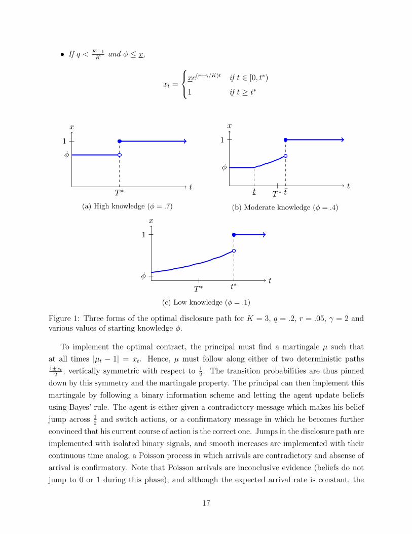
• If q < K−1K

and φ ≤ x,

xt =

xe(r+γ/K)t if t ∈ [0, t∗)

1 if t ≥ t∗

t

x

1

φ

T ∗

(a) High knowledge (φ = .7)

φ

t

x

1

T ∗t t

(b) Moderate knowledge (φ = .4)

φt

x

1

T ∗ t∗

(c) Low knowledge (φ = .1)

Figure 1: Three forms of the optimal disclosure path for K = 3, q = .2, r = .05, γ = 2 andvarious values of starting knowledge φ.

To implement the optimal contract, the principal must find a martingale µ such that

at all times |µt − 1| = xt. Hence, µ must follow along either of two deterministic paths1±xt

2, vertically symmetric with respect to 1

2. The transition probabilities are thus pinned

down by this symmetry and the martingale property. The principal can then implement this

martingale by following a binary information scheme and letting the agent update beliefs

using Bayes’ rule. The agent is either given a contradictory message which makes his belief

jump across 12

and switch actions, or a confirmatory message in which he becomes further

convinced that his current course of action is the correct one. Jumps in the disclosure path are

implemented with isolated binary signals, and smooth increases are implemented with their

continuous time analog, a Poisson process in which arrivals are contradictory and absense of

arrival is confirmatory. Note that Poisson arrivals are inconclusive evidence (beliefs do not

jump to 0 or 1 during this phase), and although the expected arrival rate is constant, the

17

conditional arrival rates are time-varying.

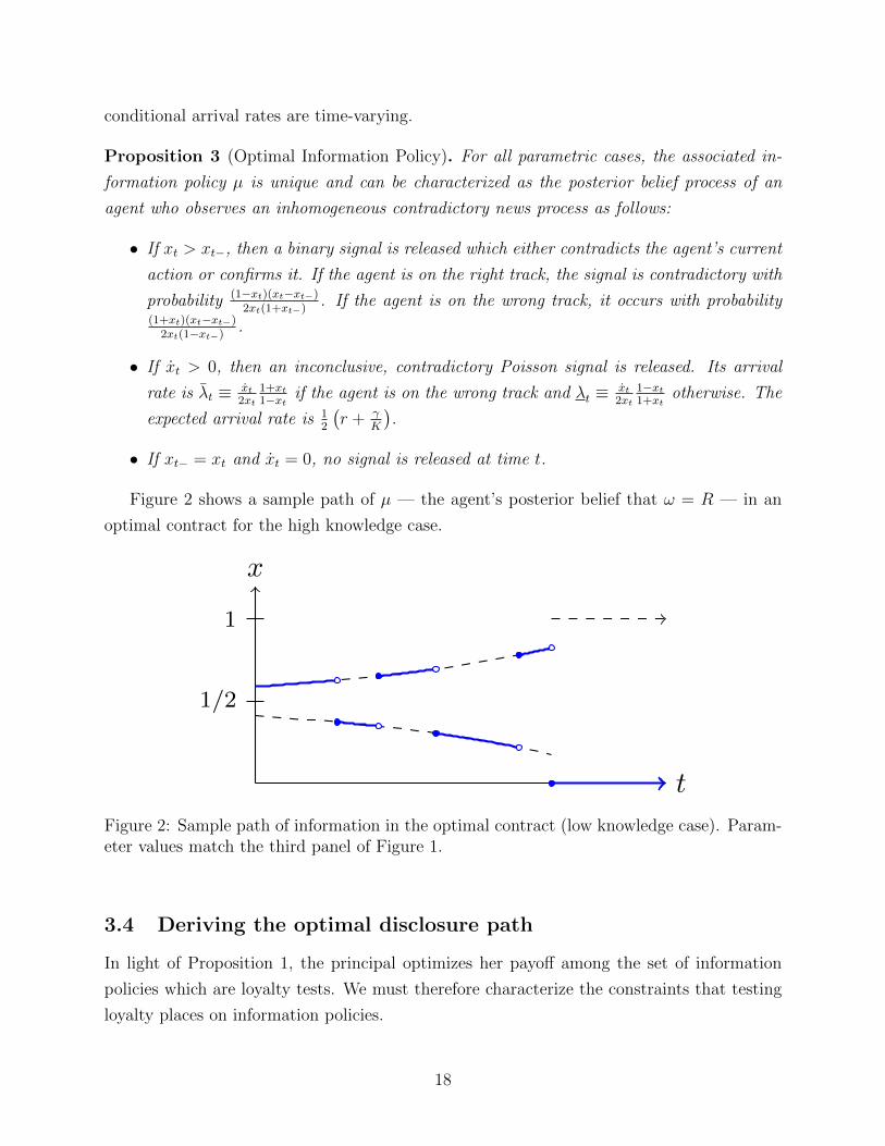
Proposition 3 (Optimal Information Policy). For all parametric cases, the associated in-

formation policy µ is unique and can be characterized as the posterior belief process of an

agent who observes an inhomogeneous contradictory news process as follows:

• If xt > xt−, then a binary signal is released which either contradicts the agent’s current

action or confirms it. If the agent is on the right track, the signal is contradictory with

probability (1−xt)(xt−xt−)2xt(1+xt−)

. If the agent is on the wrong track, it occurs with probability(1+xt)(xt−xt−)

2xt(1−xt−).

• If xt > 0, then an inconclusive, contradictory Poisson signal is released. Its arrival

rate is λt ≡ xt2xt

1+xt1−xt if the agent is on the wrong track and λt ≡ xt

2xt1−xt1+xt

otherwise. The

expected arrival rate is 12

(r + γ

K

).

• If xt− = xt and xt = 0, no signal is released at time t.

Figure 2 shows a sample path of µ — the agent’s posterior belief that ω = R — in an

optimal contract for the high knowledge case.

t

x

1

1/2

Figure 2: Sample path of information in the optimal contract (low knowledge case). Param-eter values match the third panel of Figure 1.

3.4 Deriving the optimal disclosure path

In light of Proposition 1, the principal optimizes her payoff among the set of information

policies which are loyalty tests. We must therefore characterize the constraints that testing

loyalty places on information policies.

18

Given a disclosure path x, define Ut ≡∫∞te−(r+γ)(s−t)(K−1)xs ds to be the disloyal agent’s

ex ante continuation utility at time t, supposing he has not been terminated before time t

and undermines forever afterward. The following lemma characterizes a necessary condition

satisfied by any loyalty test, which is also sufficient whenever the underlying information

policy is deterministic.

Lemma 4. Suppose x is the disclosure path of a loyalty test. Then

Ut ≤(r +

γ

K

)Ut (1)

a.e. Conversely, if µ is a deterministic information policy with disclosure path x satisfying

(1) a.e., then µ is a loyalty test.

Proof. Fix a disclosure path x corresponding to some information policy. Suppose there

existed a time t at which Ut is defined and (1) failed. Consider any undermining policy which

unconditionally sets bt = 0 from time t to time t + ε for ε > 0, and then unconditionally

sets bt = 1 after time t + ε. Let V (ε) be the (time-zero) expected continuation payoff to

the disloyal agent of such a strategy beginning at time t, conditional on not having been

terminated prior to time t. Then

V (ε) = −∫ t+ε

t

e−r(s−t)xs ds+ e−rεUt+ε.

Differentiating wrt ε and evaluating at ε = 0 yields

V ′(0) = −xt − rUt + Ut.

If V ′(0) > 0, then for sufficiently small ε the expected payoff of unconditionally undermining

forever is strictly improved on by deviating to not undermining on the interval [t, t + ε]

for sufficiently small ε > 0. (Note that undermining up to time t yields a strictly positive

probability of remaining employed by time t and achiving the continuation payoff V (ε).) So

−xt − rUt + Ut ≤ 0

is a necessary condition for unconditional undermining to be an optimal strategy for the

disloyal agent.

Now, by the fundamental theorem of calculus Ut is defined whenever xt is continuous,

and is equal to

Ut = (r + γ)Ut − (K − 1)xt.

19

As x is a monotone function it can have at most countably many discontinuities. So this

identity holds a.e. Solving for xt and inserting this identity into the inequality just derived

yields (1), as desired.

In the other direction, suppose µ is a deterministic information policy with disclosure

path x satisfying 1 a.e. To prove the converse result we invoke Lemma 9, which requires

establishing that

Ut = min{(r + γ)Ut − (K − 1)xt, rUt + xt}

a.e. By the fundamental theorem of calculus, Ut exists a.e. and is equal to

Ut = (r + γ)Ut − (K − 1)xt

wherever it exists. So it is sufficient to show that (r + γ)Ut − (K − 1)xt ≤ rUt + xt a.e., i.e.

γUt ≤ Kxt.

Combining the hypothesized inequality Ut ≤(r + γ

K

)Ut and the identity Ut = (r+γ)Ut−

(K − 1)xt yields the inequality

(r + γ)Ut − (K − 1)xt ≤(r +

γ

K

)Ut.

Re-arrangement shows that this inequality is equivalent to xt ≥ γUt/K, as desired.

Equation (1) ensures that from an ex ante perspective, at each time t the gains from

undermining at that instant must outweigh the accompanying risk of discovery and dismissal.

Thus it is surely at least a necessary condition for any loyalty test. The condition is not in

general sufficient, as incentive-compatibility might be achieved on average but not ex post

in some states of the world. However for deterministic information policies, ex ante and ex

post incentives are identical, and equation (1) is a characterization of loyalty tests. Recall

from Lemma 3 that the principal might as well choose a deterministic information policy, so

(1) may be taken as a characterization of loyalty tests for purposes of designing an optimal

policy.

In light of Proposition 1 and Lemmas 3 and 4, the principal’s design problem reduces to

solving

supx∈X

∫ ∞0

e−rtxt(q − (1− q)(K − 1)e−γt) dt s.t. Ut ≤ (r + γ/K)Ut, (PP )

where X is the set of monotone, cadlag [φ, 1]-valued functions and Ut =∫∞te−(r+γ)(s−t)(K −

1)xs ds.

The form of the constraint suggests transforming the problem into an optimal control

20

problem for U. The following lemma faciliates this approach, using integration by parts to

eliminate x from the objective in favor of U.

Lemma 5. For any x ∈ X,∫ ∞0

e−rtxt(q − (1− q)(K − 1)e−γt) dt = −(

1− K

K − 1q

)U0 +

qγ

K − 1

∫ ∞0

e−rtUt dt.

Proof. Let

Π =

∫ ∞0

e−rtxt(q − (1− q)(K − 1)e−γt) dt.

Use the fact that Ut = −(K − 1)xt + (r + γ)Ut as an identity to eliminate xt from the

objective, yielding

Π =

∫ ∞0

(q

K − 1eγt − (1− q)

)e−(r+γ)t((r + γ)Ut − Ut) dt.

This expression can be further rewritten as a function of U only by integrating by parts.

The result is

Π = −(

1− K

K − 1q

)U0 − lim

t→∞

(q

K − 1eγt − (1− q)

)e−(r+γ)tUt +

qγ

K − 1

∫ ∞0

e−rtUt dt.

Since U is bounded in the interval [0, (K − 1)/(r + γ)], the surface term at t = ∞ must

vanish, yielding the expression in the lemma statement.

The final step in the transformation of the problem is deriving the admissible set of

utility processes corresponding to the admissible set X of disclosure paths. The bounds on x

immediately imply that Ut ∈ [U,U ] for all t, where U ≡ (K − 1)/(r + γ) and U ≡ φU. It is

therefore tempting to conjecture that problem (PP ) can be solved by solving the auxiliary

problem

supU∈U

{−(

1− K

K − 1q

)U0 +

qγ

K − 1

∫ ∞0

e−rtUt dt

}s.t. Ut ≤ (r + γ/K)Ut, (PP ′)

where U is the set of absolutely continuous [U,U ]-valued functions. Any solution to this

problem can be mapped back into a disclosure policy via the identity

xt =1

K − 1

((r + γ)Ut − Ut

), (2)

obtainable by differentiating the expression Ut =∫∞te−(r+γ)(s−t)xs ds.

21

It turns out that this conjecture is correct if φ is not too large, but for large φ the

resulting solution fails to respect the lower bound x ≥ φ. To correct this problem equation

(2) can be combined with the lower bound xt ≥ φ to obtain an additional upper bound

Ut ≤ (r + γ)Ut − (K − 1)φ on the growth rate of U . This bound suggests solving the

modified auxiliary problem

supU∈U

{−(

1− K

K − 1q

)U0 +

qγ

K − 1

∫ ∞0

e−rtUt dt

}s.t. Ut ≤ min{(r + γ/K)Ut, (r + γ)Ut − (K − 1)φ}

(PP ′′)

The following lemma verifies that any solution to this relaxed problem for fixed U0 ∈[U,U ] yields a disclosure path respecting x ≥ φ. Thus a full solution to the problem allowing

U0 to vary solves the original problem.

Lemma 6. Fix u ∈ [U,U ]. There exists a unique solution U∗ to problem (PP ′′) subject to

the additional constraint U0 = u, and the disclosure policy xu defined by

xut =1

K − 1

((r + γ)U∗t − U∗t

)satisfies xu ∈ X.

We prove Proposition 2 by solving problem (PP ′′) subject to U0 = u ∈ [U,U ], and then in

a final step optimize over u to obtain a solution to problem (PP ′′) and thus to problem (PP ).

When U0 is held fixed, the objective is increasing in U pointwise, so optimizing the objective

amounts to maximizing the growth rate of U subject to the control and the upper bound

U ≤ U. The result is that U solves the ODE Ut = min{(r + γ/K)Ut, (r + γ)Ut − (K − 1)φ}until the point at which Ut = U, and then is constant afterward. Solving problem PP then

reduces to a one-dimensional optimization over U0, which can be accomplished algebraically.

4 Time Consistency

So far, we have assumed that the principal can commit at time 0 to the dynamic information

release policy. What if the principal could not commit — would she ever prefer to release

more or less information than she originally promised? In this section, we show that the

optimal contract is time consistent in a particular sense, and thus commitment power is

not necessary for the principal. For this result, we use a slightly different interpretation

of the model in which the principal does not have any private information about the state

of the world, and instead of providing information, the principal chooses the information

22

acquisition process, through which the principal and agent learn about the state together.

We show that for all parameter values, the principal’s optimal contract can be imple-

mented in a time consistent way. That is, there is an optimal strategy for the disloyal agent

such that the principal’s optimal contract is time consistent, and moreover, this strategy is

unique. While we point out that this fact would allow one to implement the optimal contract

as a Markov perfect equilibrium of a game played between the principal and agent, our focus

here is on time consistency.4

Until now, it has sufficed to consider implementations of the optimal contract in which

the disloyal agent undermines with probability one at all times. Due to the zero-sum prop-

erty, the principal is indifferent over the disloyal agent’s actions whenever the disloyal agent

is indifferent. With regard to time consistency, however, the disloyal agent’s strategy mat-

ters because it determines the posterior belief the principal has about the agent, which in

turn influences whether and how the principal would want to renegotiate the contract. In

some cases, in particular in the low knowledge and moderate knowledge cases, the optimal

contract is not time consistent under full undermining by the disloyal agent, for the following

reason. In those cases, with the disloyal agent undermining at all times, the agent’s repu-

tation reaches the critical threshold of K−1K

at time T ∗, but the optimal contract specifies

that the principal hold some information back until strictly after time T ∗. If the principal

were allowed to suddenly renegotiate at that time, she would want to release all remaining

information at once, deviating from the contract. On the other hand, in the low and mod-

erate knowledge cases, the disloyal agent is made indifferent over a range of times during

the optimal contract. By undermining with probability less than one, the agent’s reputation

conditional on not having been caught rises more slowly. With this flexibility, we can cal-

ibrate the rise in the agent’s reputation to the originally scheduled release of information,

ensuring time consistency. Hence, we let βt ∈ [0, 1] be the instantaneous probability that

the agent undermines at instant t.5

For the low and moderate knowledge cases, we identify the βt supporting time consistency

4Analyzing the game would require several technical preliminaries, including a formal notion of a strategyfor the principal without dynamic commitment along the lines of Orlov, Skrzypacz, and Zryumov (2017) andan ad hoc notion of optimality since continuation payoffs after certain off-path events are not well-definedin this kind of extensive form, continuous-time setting; for a detailed treatment of related issues, see Simonand Stinchcombe (1989).

5There are two ways to avoid technical issues with independence across instants in continuous time. Oneway is to allow the agent a unit of flow effort to allocate between undermining and cooperating, and thenβt is the fraction allocated to undermining. Alternatively, since independence of this randomization acrosstime is not necessary, we can consider randomization over cutoff times at which the disloyal agent beginsundermining forever after (and in the moderate knowledge case, where indifference begins at time t > 0, wespecify that for all realizations, the agent undermines during the interval [0, t). Under this interpretation,βt, which is increasing, is the probability that the random cutoff time is at most t.

23

in the following way. First, at each time t, we solve for the agent’s reputation qt that makes

xt the optimal starting disclosure level. From qt, we then back out βt using Bayes’ rule, and

finally we verify that the entire path of the optimal renegotiated contract given the updated

state q = qt, φ = xt overlaps with the original contract. In particular, the time of the final

information release coincides with the time at which the agent’s reputation reaches K−1K

. We

defer the full analysis of these cases to the appendix.

In the rest of this discussion, we describe why the optimal contract is already time

consistent for the case q0 ≥ K−1K

or the high knowledge case. In these cases, the agent strictly

prefers to undermine at all times in the optimal contract, so there is no scope (nor any need)

for mixing by the disloyal agent; βt is identically 1. Note that at any time in the optimal

contract, if all information has already been released, the time consistency requirement at

that time is trivially satisfied, because there is no information left to release. For the case

q0 ≥ K−1K

, the optimal contract releases all information at time 0, so clearly this is time

consistent. Note also that the disloyal agent strictly prefers to undermine at all times, so

there is a unique optimal strategy of the disloyal agent which supports time consistency.

Next, consider the high knowledge case, where the optimal contract is to wait until time

T ∗(q0) and then release all information, where we now make dependence of T ∗ on q0 explicit.

As noted above, time consistency is trivial for t ≥ T ∗(q0), so we only consider t < T ∗(q0).

Consider the (optimal) strategy of the disloyal agent of undermining at all times. Then the

principal’s posterior belief about the agent is qt = q0q0+(1−q0)e−γt

, which is strictly increasing

and reaches K−1K

at time T ∗(q0). For all t < T ∗(q0), provided that the agent has not been

caught undermining, we have xt = φ and qt <K−1K

; in other words, the continuation game

falls into the same high knowledge category as the game did at time 0. In addition, we have

T ∗(qt) = T ∗(q0) − t, so starting from time t, the optimal contract is to keep information

fixed at φ until the originally scheduled time T ∗(q0) and then release all information. This

establishes time consistency for all t < T ∗(q0). Since the disloyal agent strictly prefers to

undermine at all times, we have uniqueness.

Proposition 4. For all parameter values, there exists a unique optimal strategy of the dis-

loyal agent such that the optimal contract is time consistent. Specifically, such a strategy for

the disloyal agent is

• If q0 ≥ K−1K

or φ ≥ x(q0), βt = 1 for all t ≥ 0.

• If q0 <K−1K

and φ ≤ x(q0), βt = 1K(1−q0eγ/Kt)

for t ∈ [0, t∗) and βt = 1 for t ≥ t∗.

24

• If q0 <K−1K

and φ ∈ (x(q0), x(q0)),

βt =

1 if t ∈ [0, t)

1K(1−Ce(γ/K)(t−t))

if t ∈ [t, t)

1 if t ≥ t,

where C ≡(φx

) γγ+Kr K−1

K.

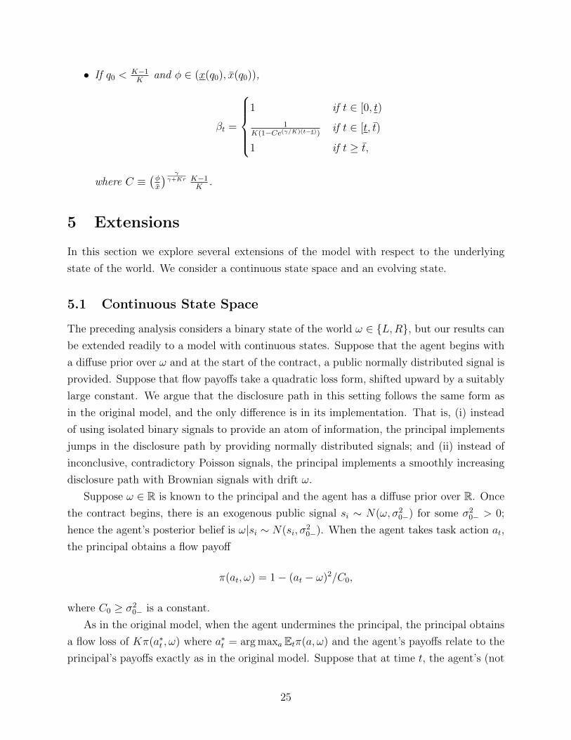
5 Extensions

In this section we explore several extensions of the model with respect to the underlying

state of the world. We consider a continuous state space and an evolving state.

5.1 Continuous State Space

The preceding analysis considers a binary state of the world ω ∈ {L,R}, but our results can

be extended readily to a model with continuous states. Suppose that the agent begins with

a diffuse prior over ω and at the start of the contract, a public normally distributed signal is

provided. Suppose that flow payoffs take a quadratic loss form, shifted upward by a suitably

large constant. We argue that the disclosure path in this setting follows the same form as

in the original model, and the only difference is in its implementation. That is, (i) instead

of using isolated binary signals to provide an atom of information, the principal implements

jumps in the disclosure path by providing normally distributed signals; and (ii) instead of

inconclusive, contradictory Poisson signals, the principal implements a smoothly increasing

disclosure path with Brownian signals with drift ω.

Suppose ω ∈ R is known to the principal and the agent has a diffuse prior over R. Once

the contract begins, there is an exogenous public signal si ∼ N(ω, σ20−) for some σ2

0− > 0;

hence the agent’s posterior belief is ω|si ∼ N(si, σ20−). When the agent takes task action at,

the principal obtains a flow payoff

π(at, ω) = 1− (at − ω)2/C0,

where C0 ≥ σ20− is a constant.

As in the original model, when the agent undermines the principal, the principal obtains

a flow loss of Kπ(a∗t , ω) where a∗t = arg maxa Etπ(a, ω) and the agent’s payoffs relate to the

principal’s payoffs exactly as in the original model. Suppose that at time t, the agent’s (not

25

necessarily normal) posterior belief has mean Mt and variance σ2t . The principal recommends

the action at = Mt, and from the disloyal agent’s perspective, the expected flow payoff from

cooperating on the task action is −xt, where

xt ≡ Et[1− (Mt − ω)2/C0] = 1− σ2t /C0.

Likewise, the disloyal agent’s expected flow payoff from undermining the principal is Kxt.

Note that xt is also the undiscounted, ex interim (i.e., conditional on ω) expected flow payoff

to the principal when the agent cooperates on the task action. Moreover, x is monotone

decreasing in σ (and hence time) and takes values in [φ, 1], where φ = 1− σ20−/C0 ≥ 0.

We can thus leverage the optimal contract from the original setting, with the only mod-

ification being to the implementation. That is, the principal commits to the exact same

disclosure path x as in the original setting, but now the information policy must be designed

according to the continuous state space.

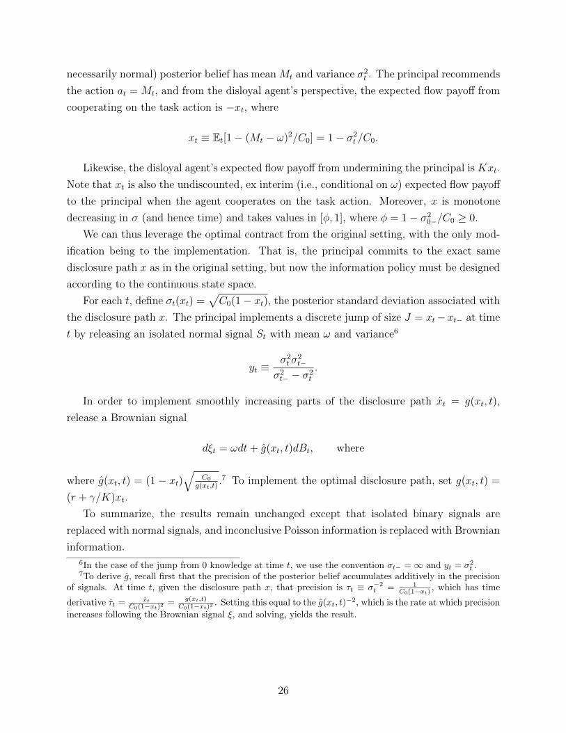
For each t, define σt(xt) =√C0(1− xt), the posterior standard deviation associated with

the disclosure path x. The principal implements a discrete jump of size J = xt−xt− at time

t by releasing an isolated normal signal St with mean ω and variance6

yt ≡σ2t σ

2t−

σ2t− − σ2

t

.

In order to implement smoothly increasing parts of the disclosure path xt = g(xt, t),

release a Brownian signal

dξt = ωdt+ g(xt, t)dBt, where

where g(xt, t) = (1 − xt)√

C0

g(xt,t).7 To implement the optimal disclosure path, set g(xt, t) =

(r + γ/K)xt.

To summarize, the results remain unchanged except that isolated binary signals are

replaced with normal signals, and inconclusive Poisson information is replaced with Brownian

information.

6In the case of the jump from 0 knowledge at time t, we use the convention σt− =∞ and yt = σ2t .

7To derive g, recall first that the precision of the posterior belief accumulates additively in the precisionof signals. At time t, given the disclosure path x, that precision is τt ≡ σ−2t = 1

C0(1−xt), which has time

derivative τt = xt

C0(1−xt)2= g(xt,t)

C0(1−xt)2. Setting this equal to the g(xt, t)

−2, which is the rate at which precision

increases following the Brownian signal ξ, and solving, yields the result.

26

5.2 Evolving State

We have assumed that the underlying state of the world is fixed, and thus the agent’s infor-

mation never becomes obsolete. Suppose that instead of being fixed over time, ω switches

between L and R in a Markov fashion with symmetric exponential transition rates λ > 0.

Any previously admissible disclosure path x remains so, and for every such disclosure path,

the principal’s and agent’s payoffs are the same as before.8 But this change in the model to

relaxes the principal’s problem by allowing the disclosure path x to be decreasing; absent

any information release, the agent’s beliefs decay asymptotically toward 12. In particular, for

parametric cases where the previous nonmonotonicity condition was binding — the princi-

pal would have prefered to withdraw information — the principal can now do this to some

extent by letting the belief temporarily decay. The old condition that xt be nondecreasing

is replaced with the weaker condition xt+s ≥ e−2λsxt for all t, s ≥ 0.

6 Discussion

In this section we briefly discuss the principal’s decision to hire the agent and conclude.

6.1 On not hiring the agent

The principal always obtains a strictly positive payoff from the optimal contract if the agent’s

starting reputation exceeds K−1K

or if the game starts in the low knowledge case. However,

in the moderate and high knowledge cases, the principal sometimes would prefer not to hire

the agent. This happens when the agent’s starting reputation is sufficiently bad given the

amount of exogenous information (either the agent’s prior knowledge or exogenous informa-

tion necessary to start the relationship). Since the principal’s payoff can be expressed in

closed form, one must simply compare it to zero to determine whether the principal should

hire the agent. This comparison yields an implicitly defined curve in (q, φ)-space above which

the principal would not hire the agent.

6.2 Conclusion

We study optimal information disclosure in a principal-agent problem when knowledge of

an underlying state of the world can be used either to aid the principal (through better job

performance) or to harm her (through leaks or sabotage). Some fraction of agents oppose

8Note, however, that now x requires more information release to adjust to the changing state. Forexample, a constant x requires a flow of information to keep the agent “up to speed.”

27

the interests of the principal, and can undermine her in a gradual and imperfectly detectable

manner. Ideally, the principal would like to keep the agent in the dark until she can ascertain

loyalty with sufficient confidence by detecting and tracing the source of any undermining.

Only after such a screening phase would the principal inform the agent about the state.

However, such an information structure gives a disloyal agent strong incentives to feign

loyalty early on by refraining from undermining, negating the effectiveness of the scheme.

We show that the principal optimally disburses information just quickly enough to dis-

suade disloyal agent from feigning loyalty at any time, maximizing the rate of detection of

disloyalty. This optimal information policy can be implemented as an inconclusive contra-

dictory news process, which gradually increases the precision of the agents information up

to a deterministic terminal date. At this date the agent is deemed trusted and a final atom

of information is released, fully revealing the state to the agent.

Our model assumes that agents are either fully aligned or totally opposed to the prin-

cipal’s long-run interests. This restriction allows us to focus on the principal’s problem of

plugging leaks by detecting and screening out disloyal agents. However, in some situations

it may be realistic to suppose that even disloyal agents can be converted into loyal ones

through sufficient monetary compensation or other incentives. We leave open as an interest-

ing direction for future work the broader question of when a principal might prefer to screen

versus convert agents who face temptations to undermine her.

A Proofs

A.1 Technical lemmas

For the lemmas in this subsection, fix a deterministic information policy µ with associated

disclosure path x.

Given any undermining policy b, define U b to be the disloyal agent’s continuation value

process under b, conditional on the agent remaining employed. By definition,

U bt =

∫ ∞t

exp

(−r(s− t)− γ

∫ s

t

bu du

)(Kbs − 1)xs ds

for all t. This function is absolutely continuous with a.e. derivative

dU b

dt= (r + γbt)U

bt − (Kbt − 1)xt.

28

Note that the rhs is bounded below by f(U bt , t), where

f(u, t) ≡ min{(r + γ)u− (K − 1)xt, ru+ xt}.

Lemma 7. Suppose g(u, t) is a function which is strictly increasing in its first argument.

Fix T ∈ R+, and suppose there exist two absolutely continuous functions u1 and u2 on [0, T ]

such that u1(T ) ≥ u2(T ) while u′1(t) = g(u1(t), t) and u′2(t) ≥ g(u2(t), t) on [0, T ] a.e. Then:

1. u1 ≥ u2.

2. If in addition u1(T ) = u2(T ) and u′2(t) = g(u2(t), t) on [0, T ] a.e., then u1 = u2.

3. If in addition u′2(t) > g(u2(t), t) on some positive-measure subset of [0, T ], then u1(0) >

u2(0).

Proof. Define ∆(t) ≡ u2(t)− u1(t), and suppose by way of contradiction that ∆(t0) > 0 for

some t0 ∈ [0, T ). Let t1 ≡ inf{t ≥ t0 : ∆(t0) ≤ 0}. Given continuity of ∆, it must be that

t1 > t0. Further, t1 ≤ T given u1(T ) ≥ u2(T ). And by continuity ∆(t1) = 0. But also by the

fundamental theorem of calculus

∆(t1) = ∆(t0) +

∫ t1

t0

∆′(t) dt.

Now, given that ∆(t) > 0 on (t0, t1), it must be that

∆′(t) = u′2(t)− u′1(t) ≥ g(u2(t), t)− g(u1(t), t) > 0

a.e. on (t0, t1) given that g is strictly increasing in its first argument. Hence from the

previous identity ∆(t1) > ∆(t0), a contradiction of ∆(t1) = 0 and ∆(t0) > 0. So it must be

that ∆ ≤ 0, i.e. u2 ≤ u1.

Now, suppose further that u1(T ) = u2(T ) and u′2(t) = g(u2(t), t) on [0, T ] a.e. Trivially

u2(T ) ≥ u1(T ) and u′1(t) ≥ g(u1(t), t) on [0, T ] a.e., so reversing the roles of u1 and u2 in the

proof of the previous part establishes that u1 ≤ u2. Hence u1 = u2.

Finally, suppose that u′2(t) > g(u2(t), t) on some positive-measure subset of [0, T ]. We

have already established that u1 ≥ u2. Assume by way of contradiction that u1(0) = u2(0).

Let t0 ≡ inf{t : u′1(t), u′2(t) exist and u′1(t) = g(u1(t), t), u′2(t) > g(u2(t), t)}. The fact that

u′1(t) = g(u1(t), t) a.e. while u′2(t) > g(u2(t), t) on a set of strictly positive measure ensures

that t0 ∈ [0, T ). By construction u′2(t) = g(u2(t), t) on [0, t0), in which case a minor variant

of the argument used to prove the first two parts of this lemma shows that u1 = u2 on [0, t0].

29

In particular, u1(t0) = u2(t0). But then by construction ∆′(t0) exists and

∆′(t0) = u′2(t0)− u′1(t0) > g(u2(t0), t0)− g(u1(t0), t0) = 0.

In particular, for sufficiently small t > t0 it must be that ∆(t) > 0, which is the desired

contradiction.

Lemma 8. Given any T ∈ R+ and u ∈ R, there exists a unique absolutely continuous

function u such that u(T ) = u and u′(t) = f(u(t), t) on [0, T ] a.e.

Proof. Suppose first that x is a simple function; that is, x takes one of at most a finite

number of values. Given that x is monotone, this means it is constant except at a finite set

of jump points D = {t1, ..., tn}, where 0 < t1 < ... < tn < T . In this case f(u, t) is uniformly

Lipschitz continuous in u and is continuous in t, except on the set D. Further, f satisfies the

bound |f(u, t)| ≤ (K − 1) + (r + γ)|u|. Then by the Picard-Lindelhof theorem there exists

a unique solution to the ODE between each tk and tk+1 for arbitrary terminal condition

at tk+1. Let u0 be the solution to the ODE on [tn, T ] with terminal condition u0(T ) = u,

and construct a sequence of functions uk inductively on each interval [tn−k, tn−k+1] by taking

uk(tn−k+1) = uk−1(tn−k+1) to be the terminal condition for uk. Then the function u defined

by letting u(t) = uk(t) for t ∈ [tn−k, tn−k+1] for k = 0, ..., n, with t0 = 0 and tn+1 = T, yields

an absolutely continuous function satisfying the ODE everywhere except on the set of jump

points D.

Now consider an arbitrary x. As x is non-negative, monotone, and bounded, there exists

a increasing sequence of monotone simple functions xn such that xn ↑ x uniformly on [0, T ].

Further, there exists another decreasing sequence of monotone simple functions xm such

that xm ↓ x uniformly on [0, T ]. For each n, let un be the unique solution to the ODE

u′(t) = fn(u, t) with terminal condition u(T ) = u, where

fn(u, t) ≡ min{(r + γ)u− (K − 1)xnt , ru+ xnt }.

(The arguments used for the case of x simple ensure such a solution exists.) By construction

fn(u, t) is increasing in n for fixed (u, t), hence dum/dt ≥ fn(um(t), t) for every m > n. Also

observe that each fn is strictly increasing in its first argument, hence Lemma 7 establishes

that the sequence un is pointwise decreasing. Then the pointwise limit of un as n→∞ is well-

defined (though possibly infinite), a function we will denote u∞. Further, fn(u, t) ≤ ru+ 1,

hence by Gronwall’s inequality un(t) ≥ −1/r + (u + 1/r) exp(r(t − T )). Thus the un are

uniformly bounded below on [0, T ], meaning u∞ is finite-valued.

30

Now define an absolutely continuous function u∗ on [0, T ] pointwise by setting

u∗(t) = u−∫ T

t

f(u∞(s), s) ds.

Our goal is to show that u∗ is the desired solution to the ODE. Once that is established,

Lemma 7 ensures uniqueness given that f is strictly increasing in its first argument.

Use the fundamental theorem of calculus to write

un(t) = u−∫ T

t

dun

dsds = u−

∫ T

t

fn(un(s), s) ds,

and take n → ∞ on both sides. Note that |fn(un(s), s)| ≤ (K − 1) + (r + γ)|un(s)|, and

recall that the sequence un is pointwise decreasing and each un satisfies the lower bound

un(t) ≥ −1/r + (u + 1/r) exp(r(t − T )). Hence a uniform lower bound on the un(t) is

min{−1/r, u}. So |un| may be bounded above by |un(s)| ≤ max{1/r, |u|, |u1(s)|}. As u1

is continuous and therefore bounded on [0, T ], this bound implies that (K − 1) + (r +

γ) max{1/r, |u|, |u1(s)|} is an integrable dominating function for the sequence |fn(un(s), s)|.The dominated convergence theorem then yields

u∞(t) = u−∫ T

t

limn→∞

fn(un(s), s) ds = u−∫ T

t

f(u∞(s), s) ds = u∗(t).

So u∞ and u∗ are the same function. Meanwhile, differentiating the definition of u∗ yields

du∗

dt= f(u∞(t), t) = f(u∗(t), t).

Then as u∗(T ) = u, u∗ is the desired solution to the ODE.

Lemma 9. An undermining policy b∗ maximizes the disloyal agent’s payoff under µ iffdUb∗

dt= f(U b∗

t , t) a.e.

Proof. Suppose first that b∗ is an undermining policy whose continuation value process U b∗

satisfies dUb∗

dt= f(U b∗

t , t) a.e. Let x∞ ≡ limt→∞ xt, which must exist given that x is an

increasing function. We first claim that lim supt→∞ Ub∗t = (K − 1)x∞/(r + γ). First, given

that xt ≤ x∞ for all time it must also be that U b∗t ≤ (K − 1)x∞/(r + γ), as the latter is the

maximum achievable payoff when xt = x∞ for all time. Suppose U∞ ≡ lim supt→∞ Ub∗t <

(K − 1)x∞/(r + γ). Then lim supt→∞ f(U b∗t , t) ≤ (r + γ)U∞ − (K − 1)x∞ < 0. This means

that for sufficiently large t, dU b∗/dt is negative and bounded away from zero, meaning U b∗

eventually becomes negative. This is impossible, so it must be that U∞ = (K−1)x∞/(r+γ).

31

Now fix an arbitrary undermining policy b with continuation value process U b. Suppose

first that at some time T, U b∗T ≥ U b

T . Then by Lemma 7, U b∗t ≥ U b

t for all t < T, and in

particular the lifetime value to the disloyal agent of b∗ is at least as high as that of b. So

consider the remaining possibility that U b∗t < U b

t for all t. Let ∆U ≡ U b0−U b∗

0 > 0. As f(u, t)

is strictly increasing in u and dU b/dt ≥ f(U bt , t) for all time, it must therefore be the case

that dU b/dt > dU b∗/dt a.e. Thus

U bt = U b

0 +

∫ t

0

dU b

dsds > U b

0 +

∫ t

0

dU b∗

dsds = U b∗

t + ∆U

for all t. But then

lim supt→∞

U bt ≥ U∞ + ∆U = (K − 1)x∞/(r + γ) + ∆U,

and as ∆U > 0 it must therefore be that U bt > (K − 1)x∞/(r + γ) for some t sufficiently

large. This contradicts the bound U bt ≤ (K − 1)x∞/(r+ γ) for all t, hence it cannot be that

U b∗t < U b

t for all time. This proves that b∗ is an optimal undermining policy for the disloyal

agent.

In the other direction, fix an undermining policy b such that dUb

dt> f(U b

t , t) on some

positive-measure set of times. Then there must exist a time T such that the equality fails on

a positive-measure subset of [0, T ]. Let U∗ be the unique solution to the ODE du/dt = f(u, t)

on [0, T ] with terminal condition u(T ) = U bT . Such a solution is guaranteed to exist by Lemma

8. And by Lemma 7, U∗0 > U b0 . So define an undermining profile b∗ by setting b∗t = bt for

t ≥ T, and

b∗t =

1, Kxt ≥ γU∗t

0, Kxt < γU∗t

for t < T. Note that the ODE characterizing U∗ may be written

dU∗

dt= (r + γb∗t )U

∗t − (Kb∗t − 1)xt.

Multiplying through by exp(−rt− γ

∫ t0b∗s ds

)allows the ODE to be written as a total

differential:

d

dt

(exp

(−rt− γ

∫ t

0

b∗s ds

)U∗t

)= − exp

(−rt− γ

∫ t

0

b∗s ds

)(Kb∗t − 1)xt.

32

Integrating from 0 to T yields

U∗0 =

∫ T

0

exp

(−rt− γ

∫ t

0

b∗s ds

)(Kb∗t − 1)xt dt+ exp

(−rT − γ

∫ T

0

b∗t dt

)U∗T .

Since U∗T = U bT = U b∗

T , this means that U∗0 is the lifetime value to the disloyal agent of

undermining policy b∗. So b is not an optimal undermining policy.

A.2 Proof of Lemma 2

We first prove the “only if” direction. Let x be the disclosure path for some information

policy µ. By assumption, µ is cadlag and thus so is x. Let F denote the filtration generated

by µ. By the martingale property, for all 0 ≤ s < t, 2µs − 1 = E[2µt − 1|Fs], and by the

triangle inequality, |2µs − 1| ≤ E[|2µt − 1||Fs]. Taking expectations at time 0 and using the

law of iterated expectations, E[|2µs − 1|] ≤ E[|2µt − 1|], and thus by definition xs ≤ xt, so x

is monotone increasing. By the same logic, we have φ ≤ xt for all t, and since µt ∈ [0, 1] for

all t, xt ≤ 1. This concludes the proof for this direction.

Next, consider the “if” direction. Suppose x is cadlag, monotone increasing and [φ, 1]-

valued; we show that there exists an information policy µ for which x is the disclosure path.

We make use of Capasso and Bakstein (2005, Theorem 2.99).

Define T ≡ {0−} ∪ [0,∞) and x0− ≡ φ and adopt the convention that 0− < t for all

t ≥ 0. We construct functions q(t1, t2, a, Y ) defined for t1, t2 ∈ T with t1 < t2, a ∈ R and

Y ∈ B(R), which will be the desired transition probabilities for µ.

Consider any pair of times (t1, t2) with 0− ≤ t1 < t2. We begin by constructing q for cases

where Y is a singleton. Define q(t1, t2, a, {y}) as follows. If xt1 = 1, set q(t1, t2, 0, {0}) =

q(t1, t2, 1, {1}) = 1 and set q(t1, t2, a, {y}) = 0 for all other (a, y) pairs. If xt2 = 0, set

q(t1, t2, a, {y}) = 1 if a = y = 12

and set q(t1, t2, a, {y}) = 0 for all other (a, y) pairs. Next

consider xt1 < 1 and xt2 > 0. For all t ∈ T , define

m±t ≡1± xt

2.

For a ∈ {m+t1 ,m

−t1}, set q(t1, t2, a, {m+

t2}) =a−m−t2m+t2−m−t2

and q(t1, t2, a, {m−t2}) =m+t2−a

m+t2−m−t2

, making

use of the fact that m+t2 −m

−t2 > 0 since xt2 > 0. Set q(t1, t2, a, {y}) = 0 for all other (a, y)

pairs.

33

Next, we extend this construction to all Borel sets Y . For any Borel set Y ∈ B(R), define

q(t1, t2, a, Y ) ≡∑

y∈Y ∩{m+t2,m−t2

}

q(t1, t2, a, {y}). (3)

Hence for all a ∈ R, for all 0− ≤ t1 < t2, q(t1, t2, a, ·) is a probability measure on

B(R). Since q(t1, t2, a, Y ) is nonzero for at most two values of a, q(t1, t2, ·, Y ) is a Borel

measurable function for all B(R) and all 0− ≤ t1 < t2. It remains to show that q satisfies

the Chapman-Kolmogorov equation, which here specializes to

q(t1, t2, a, Y ) =∑

z∈{m+t′ ,m

−t′}

(q(t1, t′, a, {z})q(t′, t2, z, Y )) ∀t1 < t′ < t2. (4)

By (3), and the fact that by construction the q(t1, t2, a, ·) are probability measures for all

t1, t2, a in the domain, it suffices to consider singletons Y ∈ {{m+t2}, {m

−t2}}. Moreover,

whenever a /∈ {m+t1 ,m

−t1}, by construction q(t1, t2, a, Y ) = 0 for all t1, t2, a in the domain

so both sides of (4) vanish and equality holds; we thus consider a ∈ {m+t1 ,m

−t1}. Note that

if m+t′ = m−t′ , then it must be that these both equal a = 1/2, and thus (4) reduces to

q(t1, t2, 1/2, {m+t2}) = q(t′, t2, 1/2, {m+

t2}). By construction, either (a) xt2 = 0 so m+t2 = 1/2

and both sides of the equation are 1, or (b) xt2 > 0 so m+t2 > m−t2 and both sides are

1/2−m−t2m+t2−m−t2

= 1/2. We conclude that (4) holds if m+t′ = m−t′ . Now whenever m+

t′ 6= m−t′ , we have

m+t2 6= m−t2 and

∑z∈{m+

t′ ,m−t′}

(q(t1, t

′, a, {z})q(t′, t2, z, {m+t2}))

=a−m−t′m+t′ −m

−t′

m+t′ −m

−t2

m+t2 −m

−t2

+m+t′ − a

m+t′ −m

−t′

m−t′ −m−t2

m+t2 −m

−t2

=a−m−t2m+t2 −m

−t2

= q(t1, t2, a, {m+t2}),

as desired. By Capasso and Bakstein (2005, Theorem 2.99), there exists a unique Markov

chain µ with q as its transition probabilities. By construction, µ is a martingale and x is its

disclosure path.

A.3 Proof of Proposition 1

Fix µ which is not a loyalty test. Without loss we take µ to be deterministic, as otherwise

Lemma 3 ensures that we may pass to a payoff-improving deterministic policy. In this case

34

it is also without loss to restrict the agent’s strategy space to undermining policies which are

deterministic functions of time. We will let xt = |2µt − 1| be the disclosure path associated

with µ.

Fix an optimal action policy b∗ for the disloyal agent under x, and let U∗ be its associated

continuation utility path. Let T ≡ inf{t : Kxt ≤ γU∗t }. If T = ∞, then dU∗/dt =

(r + γ)U∗t − (K − 1)xt a.e. by Lemma 9, and hence b∗ = 1 a.e. The optimality of such a

policy contradicts the assumption that µ is not a loyalty test. So T < ∞. And by right-

continuity of x and continuity of U∗, it must be that KxT ≤ γU∗T . Hence U∗T ≥ KxTγ≥ Kφ

γ.

Now, define a new function U by

Ut ≡

U∗t , t < T

min{U∗T exp((r + γ/K)(t− T )), (K − 1)/(r + γ)}, t ≥ T.

Further define a function x by

xt ≡1

K − 1

((r + γ)Ut −

˙U t

),

with˙U interpreted as a right-derivative when the derivative is discontinuous.

We first claim that x is a valid disclosure path. Right-continuity is by construction, so

it remains to show monotonicity and [φ, 1]-valuedness. We proceed by explicitly computing

the function. For t < T it is simply

xt ≡1

K − 1

((r + γ)U∗t − U∗t

),

and by definition U∗t = (r+ γ)U∗t − (K − 1)xt for t < T, meaning xt = xt. So x is monotone

and [φ, 1]-valued on [0, T ). Meanwhile for t ≥ T the function takes the form

xt =

γU∗TK

exp ((r + γ/K)(t− T )) , T ≤ t < T ′

1, t ≥ T ′,

where T ′ solves U∗T exp((r + γ/K)(t − T )) = (K − 1)/(γ + r). This expression is monotone

everywhere, including at the jump time T ′, where xT ′− = K−1K

γγ+r

< 1. And xT =γU∗TK

,

which is at least φ given the earlier observation that U∗T ≥ Kφ/γ. Thus given that it attains

a maximum of 1, the function is [φ, 1]-valued on [T,∞). The last remaining check is that x is

monotone at the jump time T. Recall that xT− = xT while xT =γU∗TK≥ xT , so monotonicity

holds at T as well, proving x is a valid disclosure path.

35

Next we claim that U is the continuation value process of the policy b = 1 under x, and

that b = 1 is an optimal undermining policy. The first part follows from the definition of x,

which can be re-written as the total differential

d

dt

(exp(−(r + γ)t)Ut

)= − exp(−(r + γ)t)(K − 1)xt.

Integrating both sides from t to ∞ and using the fact that limt→∞ exp(−(r + γ)t)Ut = 0

then yields

Ut =

∫ ∞t

exp(−(r + γ)(s− t))(K − 1)xs ds,

as desired.

As for the optimality of b = 1, this follows from Lemma 9 if we can show that dU/dt =

f(Ut, t) a.e., when f is defined using x as the underlying disclosure rule. Given that Ut = U∗t

and xt = x∗t for t < T, and U∗t is an optimal continuation utility process under x∗, Lemma 9

ensures the ODE is satisfied for t < T. Meanwhile for t > T, the definition of x ensures that

(r + γ)Ut − (K − 1)xt =dU

dt.

So we’re done if we can show that (r+ γ)Ut− (K − 1)xt ≤ rUt + xt, i.e. Ut ≤ Kxtγ. Using the

definition of U and the explicit form for x constructed earlier, we can read off that Ut = Kxtγ

for t < T, while Ut = K−1γ+r

< Kγ

= Kxtγ

for t ≥ T. So indeed dU/dt = f(Ut, t) a.e., and b = 1

is an optimal undermining policy under x.

The proposition will be proven if we can show that the principal obtains strictly higher

expected profits under x than under x. We just saw that U0 is the disloyal agent’s payoff

under x, and by construction U0 = U∗0 , where U∗0 is the disloyal agent’s payoff under x. So it

suffices to show that the loyal agent’s payoff is higher under x than under x.

The loyal agent’s payoff under x is just

V =

∫ ∞0

e−rtxt dt.

Let U1t ≡

∫∞te−(r+γ)(s−t)xs ds be the disloyal agent’s continuation utility process when he

undermines at all times. Then ddt

(e−(r+γ)tU1t ) = −e−(r+γ)txt, and using integration by parts

V may be rewritten

V = U10 + γ

∫ ∞0

eγtU1t dt.

36

Similarly, the loyal agent’s payoff under x may be written

V = U0 + γ

∫ ∞0

eγtUt dt,

where recall U is the disloyal agent’s continuation utility process from undermining at all

times. So we’re done if we can show that U ≥ U1 and U0 > U10 .

We first establish that U ≥ U∗. In light of Lemma 9, whenever Kxt ≥ γU∗t it must be

thatdU∗

dt= (r + γ)U∗t − (K − 1)xt ≤ (r + γ/K)U∗t ,

and whenever Kxt < γU∗t , it must be that

dU∗

dt= rU∗t + xt ≤ (r + γ/K)U∗t .

Hence dU∗/dt ≤ (r + γ/K)U∗t a.e. Then by Gronwall’s inequality,

U∗s ≤ U∗t exp((r + γ/K)(s− t))

for any t and s > t.

Now, by construction Ut = U∗t for t ≤ T, and for t ∈ [T, T ′] we have

Ut = U∗T exp((r + γ/K)(t− T )) ≥ U∗t .

Finally, for t ≥ T we have Ut = (K − 1)/(r+ γ) ≥ Ut given that (K − 1)/(r+ γ) is an upper

bound on the value of any continuation utility. So indeed U ≥ U∗.

Finally, note that trivially U∗ ≥ U1 given that U∗ is the continuation utility process of an

optimal policy, bounding above the continuation utility of an arbitrary policy at any point

in time. And by assumption U∗0 > U10 , as x is not a loyalty test. So indeed U ≥ U∗ ≥ U1

and U0 ≥ U∗0 > U1, completing the proof.

A.4 Proof of Proposition 2

We solve the first two cases by solving a relaxed version of (PP ), ignoring the IC constraint

on Ut. Note that the coefficient q − (1 − q)(K − 1)e−γt is positive iff q > (K − 1)/K or

if q ≥ K−1K

and t > T ∗, where T ∗ is defined in Section 3.3. Hence, the principal’s relaxed

problem is solved pointwise by setting xt = 1 in those cases, and by setting xt = φ otherwise.

Now if q > (K − 1)/K, we have xt = 1 for all t ≥ 0 and clearly the IC constraint is satisfied

since Ut = 0, solving the original problem and thus giving the first case of Proposition 2. If

37

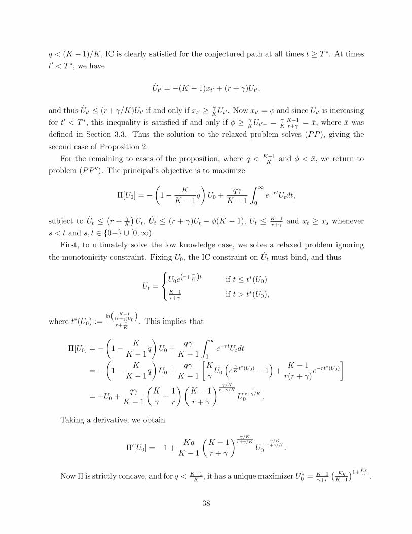
q < (K − 1)/K, IC is clearly satisfied for the conjectured path at all times t ≥ T ∗. At times

t′ < T ∗, we have

Ut′ = −(K − 1)xt′ + (r + γ)Ut′ ,

and thus Ut′ ≤ (r+γ/K)Ut′ if and only if xt′ ≥ γKUt′ . Now xt′ = φ and since Ut′ is increasing

for t′ < T ∗, this inequality is satisfied if and only if φ ≥ γKUt′− = γ

KK−1r+γ

= x, where x was

defined in Section 3.3. Thus the solution to the relaxed problem solves (PP ), giving the

second case of Proposition 2.

For the remaining to cases of the proposition, where q < K−1K

and φ < x, we return to

problem (PP ′′). The principal’s objective is to maximize

Π[U0] = −(

1− K

K − 1q

)U0 +

qγ

K − 1

∫ ∞0

e−rtUtdt,

subject to Ut ≤(r + γ

K

)Ut, Ut ≤ (r + γ)Ut − φ(K − 1), Ut ≤ K−1

r+γand xt ≥ xs whenever

s < t and s, t ∈ {0−} ∪ [0,∞).

First, to ultimately solve the low knowledge case, we solve a relaxed problem ignoring

the monotonicity constraint. Fixing U0, the IC constraint on Ut must bind, and thus

Ut =

U0e(r+ γ

K )t if t ≤ t∗(U0)

K−1r+γ

if t > t∗(U0),

where t∗(U0) :=ln(

K−1(r+γ)U0

)r+ γ

K. This implies that

Π[U0] = −(

1− K

K − 1q

)U0 +

qγ

K − 1

∫ ∞0

e−rtUtdt

= −(

1− K

K − 1q

)U0 +

qγ

K − 1

[K

γU0

(eγKt∗(U0) − 1

)+

K − 1

r(r + γ)e−rt

∗(U0)

]= −U0 +

qγ

K − 1

(K

γ+

1

r

)(K − 1

r + γ

) γ/Kr+γ/K

Ur

r+γ/K

0 .

Taking a derivative, we obtain

Π′[U0] = −1 +Kq

K − 1

(K − 1

r + γ

) γ/Kr+γ/K

U− γ/Kr+γ/K

0 .

Now Π is strictly concave, and for q < K−1K

, it has a unique maximizer U∗0 = K−1γ+r

(KqK−1

)1+Krγ .

38

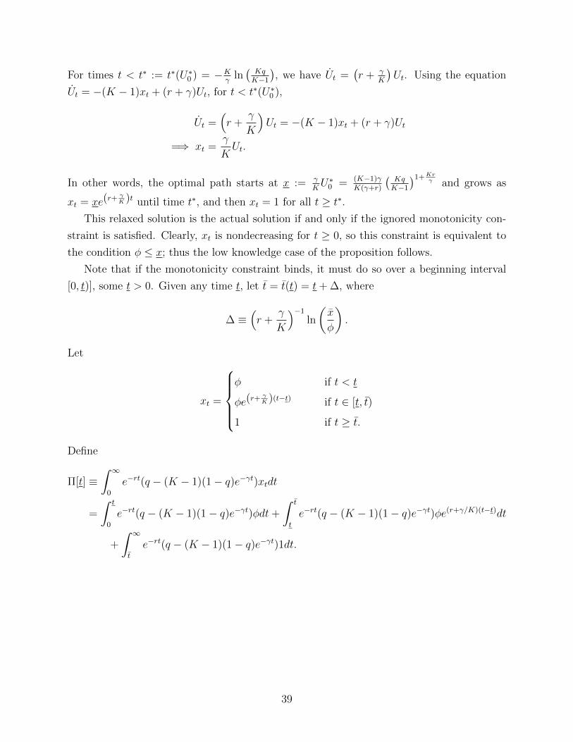
For times t < t∗ := t∗(U∗0 ) = −Kγ

ln(KqK−1

), we have Ut =

(r + γ

K

)Ut. Using the equation

Ut = −(K − 1)xt + (r + γ)Ut, for t < t∗(U∗0 ),

Ut =(r +

γ

K

)Ut = −(K − 1)xt + (r + γ)Ut

=⇒ xt =γ

KUt.

In other words, the optimal path starts at x := γKU∗0 = (K−1)γ

K(γ+r)

(KqK−1

)1+Krγ and grows as

xt = xe(r+γK )t until time t∗, and then xt = 1 for all t ≥ t∗.

This relaxed solution is the actual solution if and only if the ignored monotonicity con-

straint is satisfied. Clearly, xt is nondecreasing for t ≥ 0, so this constraint is equivalent to

the condition φ ≤ x; thus the low knowledge case of the proposition follows.

Note that if the monotonicity constraint binds, it must do so over a beginning interval

[0, t)], some t > 0. Given any time t, let t = t(t) = t+ ∆, where

∆ ≡(r +

γ

K

)−1

ln

(x

φ

).

Let

xt =

φ if t < t

φe(r+γK )(t−t) if t ∈ [t, t)

1 if t ≥ t.

Define

Π[t] ≡∫ ∞

0

e−rt(q − (K − 1)(1− q)e−γt)xtdt

=

∫ t

0

e−rt(q − (K − 1)(1− q)e−γt)φdt+

∫ t

t

e−rt(q − (K − 1)(1− q)e−γt)φe(r+γ/K)(t−t)dt

+

∫ ∞t

e−rt(q − (K − 1)(1− q)e−γt)1dt.

39

Differentiate and use that t changes at the same rate as t to obtain

Π′[t] = −∫ t

t

e−rt(q − (K − 1)(1− q)e−γt)(r + γ/K)φe(r+γ/K)(t−t)dt

− (1− x)e−rt(q − (K − 1)(1− q)e−γt)

= −(r +

γ

K

)φe−rt

K

γ

[q(eγK

∆ − 1)

+ (1− q)e−γt(e−γ(

K−1K )∆ − 1

)]− (1− x)e−rt

(qe−r∆ − (K − 1)(1− q)e−r∆e−γ(t+∆)

)=(r +

γ

K

)e−rt

[Ae−γt +B

],

where

A = −φK(1− q)γ

(e−

γ(K−1)K

∆ − 1)

+1− qr + γ

(K − 1)e−(r+γ)∆

=1− qr + γ

(K − 1)e−(r+ γK )∆

> 0

B = −φKqγ

(eγK

∆ − 1)− 1

r + γqe−r∆

= − Kq

γ(r + γ)e−r∆

(γ − φ(r + γ)er∆

)< 0.

It follows that Π′[t] is negative for sufficiently large t and positive for sufficienty low (i.e.,

negative) t. There is a unique root

t = −1

γln

(−BA

)= −1

γln

(q

1− q

(K

K − 1eγK

∆ − 1

)),

which is the optimal t and which in turn pins down t = t+ ∆.

A.5 Proof of Proposition 3

By Lemma 2, there exists an underlying information policy µ for the optimal disclosure

path x in each of the parametric cases. We now consider the three items of the proposition.

Suppose that xt > xt−. Recall that µ is a martingale and has left limits, so µt− = Et−[µt] ≡limt′↑t Et′ [µt]. Since µt takes values m±t defined in the proof of Lemma 2, it suffices to

40

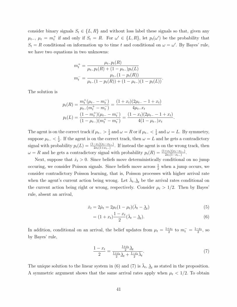
consider binary signals St ∈ {L,R} and without loss label these signals so that, given any

µt−, µt = m+t if and only if St = R. For ω′ ∈ {L,R}, let pt(ω

′) be the probability that

St = R conditional on information up to time t and conditional on ω = ω′. By Bayes’ rule,

we have two equations in two unknowns:

m+t =

µt−pt(R)

µt−pt(R) + (1− µt−)pt(L)

m−t =µt−(1− pt(R))

µt−(1− pt(R)) + (1− µt−)(1− pt(L)).

The solution is

pt(R) =m+t (µt− −m−t )

µt−(m+t −m−t )

=(1 + xt)(2µt− − 1 + xt)

4µt−xt

pt(L) =(1−m+

t )(µt− −m−t )

(1− µt−)(m+t −m−t )

=(1− xt)(2µt− − 1 + xt)

4(1− µt−)xt.

The agent is on the correct track if µt− >12

and ω = R or if µt− <12

and ω = L. By symmetry,

suppose µt− <12. If the agent is on the correct track, then ω = L and he gets a contradictory

signal with probability pt(L) = (1−xt)(xt−xt−)2xt(1+xt−)

. If instead the agent is on the wrong track, then

ω = R and he gets a contradictory signal with probability pt(R) = (1+xt)(xt−xt−)2xt(1−xt−)

.

Next, suppose that xt > 0. Since beliefs move deterministically conditional on no jump

occuring, we consider Poisson signals. Since beliefs move across 12

when a jump occurs, we

consider contradictory Poisson learning, that is, Poisson processes with higher arrival rate

when the agent’s current action being wrong. Let λt, λt be the arrival rates conditional on

the current action being right or wrong, respectively. Consider µt > 1/2. Then by Bayes’

rule, absent an arrival,

xt = 2µt = 2µt(1− µt)(λt − λt) (5)

= (1 + xt)1− xt

2(λt − λt). (6)

In addition, conditional on an arrival, the belief updates from µt = 1+xt2

to m−t = 1−xt2

, so

by Bayes’ rule,

1− xt2

=1+xt

2λt

1+xt2λt + 1−xt

2λt. (7)

The unique solution to the linear system in (6) and (7) is λt, λt as stated in the proposition.

A symmetric argument shows that the same arrival rates apply when µt < 1/2. To obtain

41

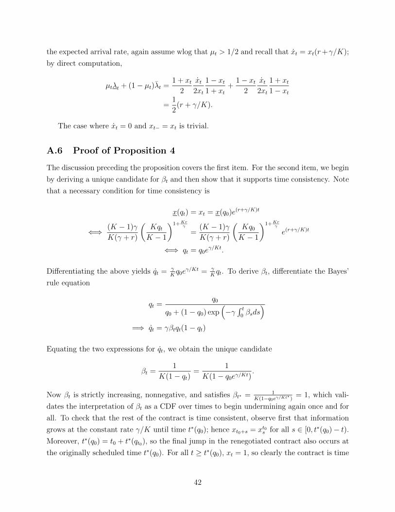
the expected arrival rate, again assume wlog that µt > 1/2 and recall that xt = xt(r+γ/K);

by direct computation,

µtλt + (1− µt)λt =1 + xt

2

xt2xt

1− xt1 + xt

+1− xt

2

xt2xt

1 + xt1− xt

=1

2(r + γ/K).

The case where xt = 0 and xt− = xt is trivial.

A.6 Proof of Proposition 4

The discussion preceding the proposition covers the first item. For the second item, we begin

by deriving a unique candidate for βt and then show that it supports time consistency. Note

that a necessary condition for time consistency is

x(qt) = xt = x(q0)e(r+γ/K)t

⇐⇒ (K − 1)γ

K(γ + r)

(KqtK − 1

)1+Krγ

=(K − 1)γ

K(γ + r)

(Kq0

K − 1

)1+Krγ

e(r+γ/K)t

⇐⇒ qt = q0eγ/Kt.

Differentiating the above yields qt = γKq0e

γ/Kt = γKqt. To derive βt, differentiate the Bayes’

rule equation

qt =q0

q0 + (1− q0) exp(−γ∫ t

0βsds

)=⇒ qt = γβtqt(1− qt)

Equating the two expressions for qt, we obtain the unique candidate

βt =1

K(1− qt)=

1

K(1− q0eγ/Kt).

Now βt is strictly increasing, nonnegative, and satisfies βt∗ = 1K(1−q0eγ/Kt∗ )

= 1, which vali-

dates the interpretation of βt as a CDF over times to begin undermining again once and for

all. To check that the rest of the contract is time consistent, observe first that information

grows at the constant rate γ/K until time t∗(q0); hence xt0+s = xt0s for all s ∈ [0, t∗(q0)− t).Moreover, t∗(q0) = t0 + t∗(qt0), so the final jump in the renegotiated contract also occurs at

the originally scheduled time t∗(q0). For all t ≥ t∗(q0), xt = 1, so clearly the contract is time

42

consistent at those times.

For the moderate knowledge case, we use a similar process. The agent strictly prefers to

undermine at all times before t and after time t. Hence undermining with certainty at those

times must be part of the disloyal agent’s strategy.

For times t ∈ (t, t), the agent is indifferent and betrays to satisfy the same equality above:

x(qt) = xt

⇐⇒ (K − 1)γ

K(γ + r)

(KqtK − 1

)1+Krγ

= φe(r+γ/K)(t−t)

⇐⇒ qt = Ce(γ/K)(t−t),

where C ≡(φK(γ+r)(K−1)γ

) γγ+Kr K−1

K=(φx

) γγ+Kr K−1

K. Again, taking derivatives, we get

qt = γβtqt(1− qt) = Cγ

Ke(γ/K)(t−t) =

γ

Kqt

⇐⇒ βt =1

K(1− qt)=

1

K(1− Ce(γ/K)(t−t)).

By inspection, βt ∈ [0, 1] is increasing; it can also be verified that qt = K−1K

and hence and

βt = 1 since. To conclude, we check time consistency. Time consistency after t(q0) is trivial

since all information has been released. Consider first t0 ∈ [0, t) and note that x(qt) = φ.

Since x is strictly increasing in q and q is strictly increasing in t, we have x(qt0) < φ < x for

all t0 ∈ [0, t(q0)). It follows that for such t0, the state (xt0 , qt0) = (φ, qt0) is in the moderate

knowledge case. It is straightforward to verify that for all t0 ∈ [0, t(q0)), t(qt0) = tq0 − t0 and

t(qt0) = tq0 − t0, which shows that xt0s = xt0+s for all s ≥ 0, establishing time consistency

for such t0. For t0 ∈ [t, t), we have qt0 <K−1K

and (by construction) xt0 = x(qt0), hence the

low knowledge case applies. It is straightforward to verify that t(qt0) = t∗(q0) − t0, hence

xt0s = xt0+s for all s ≥ 0, establishing time consistency for t0 ∈ [t(q0), t(q0)). This concludes

the proof.

A.7 Proof of Lemma 6

Fix u ∈ [U,U ]. Ignoring the fixed term involving U0 and all multiplicative constants, the

principal’s objective reduces to ∫ ∞0

e−rtUt dt,

which is increasing in the path of Ut pointwise. Let g(U) ≡ min{(r+γ/K)U, (r+γ)U−(K−1)φ}. We begin by constructing the unique pointwise maximizer of U subject to U0 = u,

43

U ∈ U, and Ut ≤ g(Ut) a.e.

Define a function U † as follows. If u = U, then set U †t = u for all time. If u ∈ (U, U)

where U ≡ Kφ/γ, then set

U †t =

e(r+γ)t(u− U

(1− e−(r+γ)t

)), t ≤ t

U exp((r + γ

K

)(t− t)

), t > t

,

where t ≡ min{

0, 1r+γ

log(U−Uu−U

)}. Finally, if u ∈ [U , U ], then set U †t = u exp

((r + γ

K

)t)

for

all time. It is readily checked by direct computation that U † satisfies U †0 = u and U †0 = g(U †t )

a.e.

Now, note that g is strictly increasing in U. By a slight variant of the arguments used

to prove Lemma 7, one can show that for any absolutely continuous function U satisfying

Ut ≤ g(Ut) a.e. and U0 = u, it must be that U † ≥ U. Further, if Ut = g(Ut) a.e., then

U = U †, and if on the other hand Ut < g(Ut) on a positive-measure set of times on any

interval [0, T ], then U †T > UT .

Define a function U∗ by U∗t = min{U †t , U}. If u = U, then the previous facts imply that

the only element of U satisfying the control constraint and U0 = u is the constant function

U∗ = U, which is then trivially the pointwise maximizer of the objective. Otherwise, note

that U † is a strictly increasing function, and there exists a unique time T at which U †t = U.

Then by the facts of the previous paragraph, U∗ is the unique pointwise maximizer of U on

the interval [0, T ] subject to the control constraint and U0 = u; and it is trivially the unique

pointwise maximizer of U subject to U ≤ U on the interval (T,∞). Thus U∗ is the unique

pointwise maximizer of U in U subject to the control constraint and U0 = u.

The final step in the proof is to show that the disclosure path implied by U∗ lies in X.

Let

x∗t ≡1

K − 1

((r + γ)U∗t − U∗t

).

If u = U, then x∗ = φ, which is in X. Next, if u ∈ (U, U) then

x∗t =

φ, t ≤ t

φ exp((r + γ

K

)(t− t

), t < t < T

1, t ≥ T.

Note that x∗T = 1 while x∗T− = γKK−1r+γ

< 1. So x∗ is monotone increasing, bounded below by

44

x∗0 = φ and above by 1. So x ∈ X. Finally, if u ∈ [U , U), then

x∗t =

uγK

exp((r + γ

K

)t), t < T

1, t ≥ T.

Given u ≥ U , uγ/K ≥ φ, so x∗ is monotone increasing at t = 0. And at t = T it satisfies

x∗T = 1 and x∗T− = γKK−1r+γ

< 1. Thus x∗ is monotone increasing everywhere, bounded below

by x∗0 = uγ/K ≥ φ and above by 1. So x ∈ X.

References

Ball, Ian (2018). Dynamic Information Provision: Rewarding the Past and Guiding the Fu-

ture. In:

Capasso, Vincenzo and David Bakstein (2005). An introduction to continuous-time stochastic

processes. In: Birkhauser Boston, p. 1.

Che, Yeon-Koo and Konrad Mierendorff (2017). Optimal sequential decision with limited

attention. Working paper.

Cranley, Ellen (2018). A senior White House aide is reportedly sharing fake stories with

staffers to identify who’s leaking to the press. In: Business Insider. url: https://www.

businessinsider.com/trump-leaks-leakers-2018-6.

Daley, Brendan and Brett S Green (2018). Bargaining and News. Working paper.

Ely, Jeffrey (2017). Beeps. In: The American Economic Review 107.1, pp. 31–53.

Ely, Jeffrey and Martin Szydlowski (2017). Moving the Goalposts.

Fudenberg, Drew and Luis Rayo (2018). Training and Effort Dynamics in Apprenticeship.

Gratton, Gabriele, Richard Holden, and Anton Kolotilin (2017). When to Drop a Bombshell.

Gryglewicz, Sebastian and Aaron Kolb (2018). Strategic Pricing in Volatile Markets. Working

paper.

Guo, Yingni and Eran Shmaya (2017). The interval structure of optimal disclosure. Working

paper.

Horner, Johannes and Andrzej Skrzypacz (2016). Selling information. In: Journal of Political

Economy 124.6, pp. 1515–1562.

Isaac, Mike (2016). Facebook ‘Trending’ List Skewed by Individual Judgment, Not Insti-

tutional Bias. In: The New York Times. url: https://www.nytimes.com/2016/05/

21/technology/facebook-trending-list-skewed-by-individual-judgment-not-

institutional-bias.

45

Kamenica, Emir and Matthew Gentzkow (2011). Bayesian persuasion. In: The American

Economic Review 101.6, pp. 2590–2615.

Kinery, Emma (2017). As Jeff Sessions Announces Leak Crackdown, Here are 12 Major

Leaks of the Trump Era. In: USA Today. url: https://www.usatoday.com/story/

news/politics/onpolitics/2017/08/04/here-12-major-leaks-donald-trump-

era/539674001.

Kolodny, Lora (2018). Elon Musk Emails Employees about ‘Extensive and Damaging Sabo-

tage’ by Employee. In: CNBC. url: https://www.cnbc.com/2018/06/18/elon-musk-

email-employee-conducted-extensive-and-damaging-sabotage.html.

Kolotilin, Anton et al. (2017). Persuasion of a privately informed receiver. In: Econometrica

85.6, pp. 1949–1964.

Orlov, Dmitry, Andrzej Skrzypacz, and Pavel Zryumov (2017). Persuading the Principal To

Wait. Stanford University Working Paper.

Rothschild, Neal (2018). The 16 Juiciest White House Leaks of 2018. In: Axios. url: https:

//www.axios.com/white-house-leaks-president-trump-2018-92899c04-0dfe-

4b64-bc42-18fcdb09e28f.

Simon, Leo K and Maxwell B Stinchcombe (1989). Extensive form games in continuous time:

Pure strategies. In: Econometrica: Journal of the Econometric Society, pp. 1171–1214.

Thompson, Nicholas and Fred Vogelstein (2018). Inside the Two Years That Shook Facebook

- and the World. In: Wired. url: https://www.wired.com/story/inside-facebook-

mark-zuckerberg-2-years-of-hell.

Watson, Joel (2002). Starting small and commitment. In: Games and Economic Behavior

38.1, pp. 176–199.

Zhong, Weijie (2017). Optimal Dynamic Information Acquisition. Working paper.

46