MASTER’S THESIS

2006:239 CIV

MARCUS HEINCKE

Leaking Rear AxlesA Design for Six Sigma Project at General Motors

MASTER OF SCIENCE PROGRAMMEIndustrial Economics

Luleå University of TechnologyDepartment of Business Administration and Social Sciences

Division of Quality & Environmental Management

2006:239 CIV • ISSN: 1402 - 1617 • ISRN: LTU - EX - - 06/239 - - SE

i

Preface This Master’s Thesis is the last part of my education in Industrial Management and Engineering with concentration towards Quality Technology and Management at Luleå University of Technology. The thesis is conducted at General Motors Corporation in Detroit during late fall and winter of 2005. The written report has been conducted in Sweden during the first half of 2006. I would like to express my gratitude to Bo Anderson for giving me the opportunity to do my Master’s Thesis at GM. Special thanks goes to my supervisor at GM, Jim Pastor, for giving me excellent guidance and always lending me a helping hand when needed, both during my time in Detroit as well as when writing the report back in Sweden. I would also like to thank Thomas Nejman for helping me with practical things before and during my stay and for taking good care of me during my time in Detroit. Also big thanks to Rickard Garvare, my supervisor at Luleå University of Technology, for excellent feedback and support during the project. During my time at GM I met a lot of people who helped me out a lot with their expertise and knowledge. Glen Pruden, Dave Teichman, Kevin Frontera, Mike Palecek and Scott Neher, thank you very much for your help. From American Axle & Manufacturing I would like to give special thanks to John Sofia for facilitating my work at their plant. I would also like to thank Jami Pole and Steve Wasik for taking the time to assist me during my visits at AAM and for providing me with information and data.

Luleå, June 2006

............................................. Marcus Heincke

ii

Sammanfattning Det problem som behandlats under detta projekt är att några av bakaxlarna till General Motors modeller GMT800 och GMT900 läcker. De flesta av läckorna påträffas redan vid målningen hos Paint Tech International (PTI), men några kommer hela vägen till kund innan de upptäcks. Läckorna uppenbarar sig normalt som en våt fläck kring ventilområdet på differentialen, eller i värre fall som en samling av olja i flänsen kring kardanknuten. Läckan hade sedan tidigare isolerats till gränsytan mellan ventilen och en plastkork som täcker den under tillverkning och montering. Detta är ett Design for Six Sigma projekt och följer IDDOV cykeln. IDDOV erbjuder ett systematiskt angripssätt för att hitta och eliminera orsaker till variation. IDDOV står för Identify (Identifiera), Define (Definiera), Develop (Utveckla), Optimize (Optimera) och Verify (Verifiera). Syftena med projektet är att komma underfund med varför somliga axlar läcker och föreslå en design- eller processändring för att reducera antalet läckande axlar. Läckagets position verifierades och projektets strategi bestämdes i projektets första fas. Projektet bröts ned i två kategorier; processtudie och designstudie. I processtudien gjordes jämföranden mot axlar av andra storlekar och eventuella skillnader mellan GMs olika monteringsanläggningar. I designstudien gjordes ett duglighetstest, som visade på brister hos ventilen, korken och oljemängden i varje axel. En komponentsökning utan tillförlitliga resultat utfördes också här. Det mest intressanta fyndet kom från processtudien som påvisade skillnader i tillverkningsprocessen mellan 8,6” axeln och 11,5” axeln. 11,5” axeln fick nya fräscha korkar efter att den blivit målad, för att försäkra att trycket i axeln hade utjämnats. För att se om ventil-kork-paren påverkas av värmen som de utsätts för i tillverkningsprocessen, gjordes ett försök i två steg. Första steget för att se om värme hade påverkan på korken, och den andra delen utfördes senare, med ytterliggare faktorer, för att precisera påverkan på korken. Från försöket kom det fram att värme och tid båda påverkar det erforderliga trycket som krävs för att skjuta av korken från ventilen. Därmed är det bevisat att korken försvagas av värmebehandlingen i ugnen. En processförbättring gjordes tidigt i projektet. Samtliga 8,6” axlar får numera sina korkar avdragna ett par sekunder hos PTI. Korken återplaceras senare när trycket i axeln har utjämnats. Sedan processändringen har det funnits regelbunden kommunikation med GM, för en försäkran om att inga axlar läcker längre. GM utförde även ett sannolikhetstest för att bekräfta att det inte längre finns läckande axlar. Den totala summan som uppskattats ha sparats in av projektet är kring $ 29 000. Förslag till processändring, baserade på projektets resultat, är att fortsätta med den påbörjade arbetsuppgiften att dra av och återplacera korken hos PTI. Helst bör en ny kork användas istället för den gamla, detta för att separera de tryckutjämnade axlarna från de som inte tryckutjämnats, och också för att korken tar skada av värmen den utsätts för tidigare i tillverkningsprocessen.

iii

Abstract The issue for the project is that some of the rear axles for General Motors GMT800 and GMT900 are found to be leaking. Most of the leaks are spotted already at the paint facility Paint Tech International (PTI), but some make it all the way to the customer before being spotted. The leaks are normally discovered as a wet spot around the vent tube area on the differential, or in more severe cases as a puddle of lube around the pinion flange. The leak has already been isolated to the interface between the vent and a plastic cap covering it during manufacturing and assembling. The project is a Design for Six Sigma project, and follows the IDDOV cycle. IDDOV offers a systematic approach to find and eliminate causes of variation in a process. IDDOV stands for Identify, Define, Develop, Optimize and Verify. The purposes of this project are to find out why some axles leak and to suggest a design or process change to reduce the number of leaking axles. The area of the leaks was verified and the strategy to be used was decided in the projects phase. The project was broken down into two categories; process study and design study. The process study made comparisons against axles of other sizes as well as differences between different GM assembly plants. In the design study a capability study was made, which showed some shortcomings in the vent, cap and the amount of lube injected in each axle. A component search without any reliable results was also done here. The most interesting finding was from the process study which showed differences in the manufacturing processes between the 8.6” axle and the 11.5” axle. The 11.5” axle got new fresh caps after the paint process to make sure the axle had been pressure equalized. To find out if the vent and cap pairs are affected by the heat that are applied to them in the manufacturing process, a design of experiments was made in two steps. The first step was to see if heat had an impact, and the second step was later done, with some additional factors, to more precisely determining the impact. From the study, heat and time in the oven were found to impact the amount of pressure it takes to pop off the plastic cap of from the vent. By that it is known that the heat treatment is weakening the cap. A process improvement was made early in the project. All 8.6” axles have now their caps pulled for a few seconds at PTI. The cap is then replaced when the pressure inside the axle has been equalized. Since the process change, interaction has been held with GM regularly to make sure no axles leak anymore. GM has also made a test to confirm that the axles do not leak anymore. The total amount of savings from the project is estimated to be about $ 29,000. The suggestion for process change, based on the findings of the project, is to continue with the ongoing task of removing and replacing the caps at PTI. Preferably a new cap should be used instead of the old one, to separate the equalized axles from the non-equalized ones, and also since the cap does get deformed by the heat earlier in the manufacturing process.

iv

Table of Contents

1 INTRODUCTION 1

1.1 THE COMPANY - GENERAL MOTORS CORPORATION 1 1.2 THE PRODUCT - REAR AXLE 2 1.3 PROBLEM DISCUSSION 2 1.4 PURPOSE AND DELIMITATION 3

2 METHODOLOGY 5

2.1 THE CHOSEN METHOD 5 2.2 DATA GATHERING 5 2.3 SIX SIGMA 5 2.4 SIX SIGMA VS. DESIGN FOR SIX SIGMA 6 2.5 CRITICAL TO QUALITY 9 2.6 DESIGN OF EXPERIMENTS 9 2.7 STATISTICAL PROCESS CONTROL 12 2.8 CAPABILITY 13 2.9 RED X 14 2.10 HYPOTHESIS TEST 16

3 THEORETICAL FRAME OF REFERENCE 19

3.1 THE HISTORY OF QUALITY 19 3.2 COST OF POOR QUALITY 19 3.3 THE HISTORY OF SIX SIGMA 20

4 EMPIRICAL STUDIES 21

4.1 IDENTIFY AND DEFINE 21 4.2 DEVELOP CONCEPTS 24 4.3 OPTIMIZE THE DESIGN 40 4.4 VERIFY THE DESIGN 45

5 CONCLUSIONS 46

5.1 SUGGESTIONS 47 5.2 COSTS AND SAVINGS 47

6 DISCUSSION 48

7 REFERENCES 50

7.1 PRINTED SOURCES 50 7.2 INTERNET SOURCES 50 7.3 INTERNAL DOCUMENTS 51

v

Table of Appendices

APPENDIX 1 – FLOW CHARTS

APPENDIX 2 – PROBLEM DEFINITION TREE

APPENDIX 3 – PROJECT DEFINITION TREE

APPENDIX 4 – EARLY MILEAGE DIVIDED UP IN PLANTS

APPENDIX 5 – TRANSPORTATION

APPENDIX 6 – CAPABILITY STUDY

APPENDIX 7 – DESIGN OF EXPERIMENTS

APPENDIX 8 – NEW FLOW CHART FOR PTI

APPENDIX 9 – BINOMIAL PROBABILITY

APPENDIX 10 – REAR AXLE OIL SEEPAGE AT VENT CAP

Introduction

1

1 Introduction This chapter introduces the reader to the project in question. It starts off with a brief view of the history of Detroit and narrows down to General Motors Corporation and finally onto the specific issue. In the end the purposes of the project as well as the delimitations are stated. The area where modern Detroit lies today has been an important trading region between different Native American tribes for several hundreds of years. In fact, it was so important that only traders were allowed to enter into the territory. Detroit’s journey to a modern city started to take shape roughly 300 years ago when French explorer Antoine de la Mothe Cadillac landed on the banks of the Detroit River and established a fort. In 1760 French rule gave away for British, and in 1796 Detroit became American as a result of Jay’s Treaty. Detroit was incorporated as a city in 1815 and became well known for the manufacturing of cigars and kitchen assortments. In 1896 Henry Ford built his first car in Detroit, and following that dozens of different motor companies emerged in the early 20th century. Not surprisingly, Detroit holds on to some of the milestones in the automotive history such as the world first mile of concrete highway built in 1909, the U.S. first traffic light installed in 1915, the nation’s first urban freeway built in 1942, and shares the worlds first traffic tunnel between two nations – the Detroit/Windsor tunnel. (www.visitdetroit.com)

1.1 The Company - General Motors Corporation General Motors Corporation (GM) was founded in 1908 when William Crapo "Billy" Durant of Durant-Dort Carriage Company incorporated the Buick Motor Company. Since 1931 GM has been the world’s largest automaker and employs today 317,000 people around the world and has manufacturing in 32 different countries. Through World War II GM transformed their production to the war effort and delivered more than $ 12.3 billion worth of material to the Allies. In 1971 GM designed and manufactured the mobility system for the Lunar Roving Vehicle which enabled the Astronauts onboard Apollo 15 to make the first vehicular drive on the moon. During 2005 GM sold close to 9.2 million cars and trucks, the second-highest total in the company’s history, and had a turn-over of almost $ 193 billion. GMs global headquarters is the GM Renaissance Center in Detroit, Michigan. Today, GM's automotive brands are Buick, Cadillac, Chevrolet, GMC, Holden, Hummer, Opel, Pontiac, Saab, Saturn and Vauxhall. (www.gm.com) There are countless of suppliers to GM. Only for the upcoming GMT900 (General Motors Trucks) series, there are approximately 1100 different suppliers according to GMT900 Supplier Quality and Launch manager Jim Pastor.

1.1.1 The Supplier - American Axle & Manufacturing American Axle & Manufacturing (AAM) was founded in 1994 by Richard E. Dauch. Once a part of GM, AAM has more than 80 years of experience in design, engineering, validation and manufacture of driveline systems, chassis systems, and forged products for trucks, bus, sport utility vehicles, and passenger cars. They have more than 12,000 associates and 17 manufacturing sites located in the US, Brazil, Mexico and United Kingdom. During 2005 AAM’s net sales were close to $ 3.4 billion. Their global headquarters is located in Detroit, Michigan. (www.aam.com)

Introduction

2

1.2 The Product - Rear Axle Axles are an important part of any wheel driven vehicle since they maintain the position between the wheels relative to each other and to the vehicle body. The wheels are also the only things touching the ground, and therefore the axles must be able to bear the weight of the vehicle and its cargo as well as withstanding the acceleration forces. In addition of the structural purposes, axles in general have different purposes depending on the design of the vehicle. These purposes are drive, braking and steering. (www.wikipedia.org) On rear axles, as the one displayed in Figure 1-1, the power from the engine comes into the differential through the pinion nose. Inside the differential the force is distributed to the two wheels, each attached to a separate shaft. This allows for independent suspension of the wheels and provides a smoother ride. It also permits the wheels to rotate at different speeds which improve traction and longer tire life. (www.wikipedia.org)

Figure 1-1 Sketch of a rear axle

1.3 Problem Discussion As GM prepares for the start of production of the new Full Size Trucks and Utilities for 2006, one of the parts Engineering and Supplier Quality has been struggling with is the rear axles. This particular part successfully completed component and subsystem validation testing, however periodically GM discovered an axle or a vehicle at the GM Assembly Plant which showed fluid on the axle. GM does not know why some axles leak while others do not. There are two supplier manufacturing locations for the rear axle. One is located in Guanajuato, Mexico (GGA) and one is located in Detroit, Michigan (DGA). From GGA axles are shipped to Arlington Texas and Silao Mexico. From the DGA axles are sent to Flint Michigan, Pontiac Michigan, Oshawa Canada, Janesville Wisconsin, Fort Wayne Indiana and Arlington Texas. According to the warranty data, all plants seem to have a problem with this issue. The warranty data also shows that leaks around the specific problem area costs GM about $ 58, 500 annually, and maybe more. According to lead design engineer for the

Introduction

3

GMT900 axles Mike Palecek, leaking axles is the primary reason a customer takes back an axle for warranty repair. Manufacturing the axles starts off with the construction and assembling of the differential. When that is done the differential is pressure tested to make sure there are no leaks. When the differential is done the tubes are put on place and welded to the differential. Additional assembling like speed sensors, cover pan and brakes are done before the axle is pressure tested again. Following that, the axles is filled with oil, sealed and shipped of for painting. At the paint facility the axles are washed, blow-dried and masked before being painted. When the painting is done the axles are dried in an oven before being unloaded and stored until shipped off to different sequencers for GM assembly plants all over the US and Canada. At the sequencers different tasks are performed depending on which plant the axles are being shipped to. In Appendix 1 there are some flow charts that show the processes of the axles with some more detail. The problem area has been isolated to a vent tube that is located on the differential. The vent tubes purpose is to release pressure that is built up inside the differential. During shipping to and from painting as well as during the paint process, a yellow plastic cap is placed above the vent tube in order to prevent dirt and filth from getting inside the differential as well as to avoid lube from leaking out of the differential. During shipping, the axles are carried in large racks and when one axle leaks the lube will drop down onto the axle below. At the assembly plant the cap is removed and replaced with a hose. The hose has almost the same purpose as the cap, allowing variations of pressure within the differential. The hose is about three feet long and ends up around the gas cap. Since the end is high up in the vehicle, the differential can be submerged without having water leaking into it. This is useful in situations like launching boats. The majority of the leaking axles are found at the paint facilities or at GMs assembly plants, but occasionally customers complain about leaks around the vent tube area. Since it is mainly an internal problem within production, it is hard to fully estimate the exact extension of the problem. Breakdown from labor codes show that leakages from the differential after sales lay around an average of 0.8 Incidents Per Thousand Vehicles (IPTV) for all axles. This is approximately equal to a sigma level of about 3.9 for the axles that are found leaking by customers. All axles reported do in fact not leak. Many of them have lube left on them from a leaking axle above during shipping to the GM Assembly Plant. The customer often sees lube on the axle and assumes the axle is leaking.

1.4 Purpose and Delimitation The axles should be manufactured in a way so that no leakage occurs. This can likely be done by design changes, process changes, or both. The purposes of this project are;

• To investigate why some rear axles leak • To suggest process or design changes in order to reduce the number of leaking

rear axles Depending on the type of the vehicle different axles are needed. For GM this results in a countless number of different axles. The problem with the leaking axle has

Introduction

4

mainly been an issue on the 8.6” axle for GMT800 and for the launch of the GMT900, but there is no evidence saying that other axles do not experience the same problem. The current production of axles is mainly for the GMT900, but there is still production going on for the GMT800. For that reason, the focus on this project will be on the 8.6” axles for GMT800 and GMT900.

Methodology

5

2 Methodology This chapter explains the methodologies and tools used to reach the purposes for the project. It starts with a brief explanation of the chosen method. From there the focus is on each specific method or tool used, and in the end there is an explanation of and a discussion about reliability and validity for the project.

2.1 The Chosen Method This project is conducted as a Design for Six Sigma, DFSS, project. Traditional Six Sigma is a systematic approach to problem solving (Bergman and Klefsjö 2003, p 545) but the difference between DFSS and Six Sigma is according to Chowdury (2002, p 1) that Six Sigma focuses on streamlining the production and business process to eliminate mistakes and save money, while Design for Six Sigma starts earlier, to develop or redesign the process itself. That way fewer downstream errors occur. The project is mainly conducted as a case study with some elements of experimental methodology. According to Bell (2000, p 16) case studies are suitable when the researcher is working by him or herself, since that opens up possibilities to investigate a problem in depth. Bell quotes Adelman et al (1977) that say that case studies is a name for a group of methodologies that have in common that they focus on one particular phenomenon. Experiments make it possible to draw conclusions about cause and effect (Bell 2000, p 21).

2.2 Data gathering To be able to get a better understanding of the issue and the processes involved with the manufacturing of axles and the assembling of the trucks, there has been constant contact with AAM and people within GM during the whole project. A number of visits to AAM and their paint facility, as well as to different GM assembly plants have also eased the understanding of the product and its processes. The literature studies have mainly been conducted through the use of Internet and search engines such as Emerald and Ebsco. An online library known as ebrary have also been used along with the library at Luleå University of Technology. In addition to that, information has been collected from GMs intranet, the Socrates.

2.3 Six Sigma Unwanted variation is a source of costs and unsatisfied customers, and by eliminating or drastically reduce the variation that is important for the customer, huge savings can be made (Bergman et al 2001, p 548). Originally stated by Minitab Inc, Caulcutt (2001, p 302) uses the definition; “Six Sigma is an information-driven methodology for reducing waste, increasing customer satisfaction and improving processes, with a focus on financially measurable results.” to describe Six Sigma. When a process reaches Six Sigma it averages 3.4 defects per million opportunities (Bergman et al, 2001, p 548). Sigma is originally a letter from the Greek alphabet and is written as σ, and it denotes the standard deviation (Bergman et al 2001, p 548). For a process that is normal distributed and in statistical balance to be Six Sigma, the distance from the process average to the closest tolerance limit must be six times the standard deviation. Most of the time a process is interrupted by variation, both natural variation, which is present when the process is in statistical balance, and statistical variance. If this

Methodology

6

variation is not too big, it can be accepted according to the Six Sigma way, as long as the variation does not go beyond ±1.5σ from the target value. Figure 2-1 displays the normal distribution and the ±1.5σ shift. The probability for defects during these conditions is 0.0000034 or 3.4 defects per million opportunities (DPMO). (Bergman et al 2001, p 548f) General Electric defines an “opportunity” as a chance for nonconformities, or not meeting the required specifications (General Electric).

Figure 2-1 The Normal Distribution with the ±1.5 σ shift (from Bergman et al, 2001 p 549) To get a better understanding of the significance of the sigma value, the connection between them and DPMO are shown in Table 2-1. Table 2-1 Sigma value transformed into DPMO (from Caulcutt 2001, p 303).

Sigma to DPMO A 3σ process produces less than 66 810 DPMO A 4σ process produces less than 6 210 DPMO A 5σ process produces less than 233 DPMO A 6σ process produces less than 3.4 DPMO

Improvement projects are supported by two improvement methodologies, one for process improvement (Six Sigma) and one for design improvement (Design for Six Sigma, DFSS) (Magnusson et al 2003, p 56). According to Magnusson et al (2003, p 58f) Six Sigma embodies a distinct process improvement methodology that is systematic, easy-to-use and formalized. The methodology consists of five phases, together known as DMAIC. DMAIC stands for Define, Measure, Analyze, Improve and Control. For design improvements the cycle is known as DMADV, Define, Measure, Analyze, Design and Verify (Magnusson et al 2003, p 59) or IDDOV, Identify, Define, Develop, Optimize, and Verify (Chowdhury 2002, p 18).

2.4 Six Sigma vs. Design for Six Sigma Berryman (2002, p 23) sees DFSS as the solution when companies run out of easy ways to find and fix defects, or in other words when Six Sigma does not work anymore. This is known as the “4-sigma” wall, and to be able to get by it companies need to use DFSS (Berryman 2002, p 24). Instead of the “4-sigma”, wall Bañuelas and Antony (2004, p 250) say that many companies reach five-sigma level, but not

Lower tolerance limit

Upper tolerance limit

Target value

4.5 σ 4.5 σ 1.5 σ 1.5 σ 6 σ 6 σ

Methodology

7

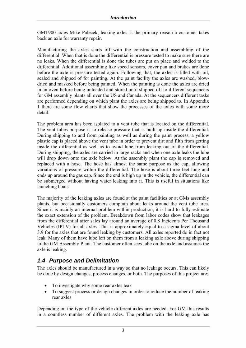
beyond. The only way to go beyond five-sigma is to implement DFSS (Bañuelas et al 2004, p 250). By implementing DFSS the organizations are not only fixing the problems as they occur, they try to find why there is a problem and where the problem is, thus attacking the problem at its source. Chowdhury (2002) points to the fact that most companies only spend about 5 percent of their budget on design, when design accounts for about 70 percent of the cost of the product, because 80 percent of the quality problems are actually designed into the product. A recognized fact about costs of poor quality is that the later in the product life cycle problems are discovered, the higher the cost to correct the problems. (Berryman 2002, p 24) This is illustrated in Figure 2-2.

Figure 2-2 Where Six Sigma Activity Occurs (from Berryman 2002, p 24)

2.4.1 IDDOV Methodology Chowdhury (2002, p xvi) points out that there are many methodologies to follow within DFSS. DMADV, DMEDI and IDDOV are some of them, but it does not really matter which one is followed, since they all are straight forward, five-step process, just like the DMAIC cycle of Six Sigma.

2.4.1.1 Identify and Define Opportunity The function of the first step in IDDOV is to provide strong, clear directions for the work to come. This phase is crucial since every activity in the continuation of the process will be based upon it. A small mistake here will have severe effects further down the road. The two primary objectives for the ID-phase is

• Get the project started on the right foot • Clearly define the requirements for which the team is aiming

(Chowdhury 2002, p 71)

Identify Phase Chowdhury (2002, p 72) points to developing a project charter, translating the Voice of the Customer into design requirements and identifying Critical to Quality (CTQs) as the three main objectives in the identify phase.

Research

Design

Prototype

Production

Custom

er

Most current Six Sigma effort is here – in production and delivered quality.

Must move quality efforts here!

Cos

t to

corr

ect d

efec

ts

Methodology

8

Define Phase This part of the IDDOV is about clearly defining the requirements of the product. The primary method of accomplishing this is Quality Function Deployment (QFD). The information from the QFD provides critical information and directions for the upcoming phases. (Chowdhury 2002, p 85f) Dr. David Woodford have identified the most important tools in the first two steps of the IDDOV cycle to be among others; QFD, Failure Means and Effects (FMEA) and Target Costing and Benchmarking. (http://www.isixsigma.com) In this project none of the mentioned tools above have been used. Instead other tools such as concentration diagram, brainstorming and strategy diagram have been used, after discussion with Jim Pastor. These tools were found to be just as fine, but more time efficient and easier to grasp.

2.4.1.2 Develop Concepts From the first phase, the prioritized customer requirements and targets are received. When these things are known, the next step is to find out if there is a product/service in mind, and if so does it meet the requirements and targets set up by the customers. If that is not the case, a new concept that could have a chance has to be developed. The most important output from the developing phase is a concept that not only meets customer requirements, but also is free of failure potential. In this phase, Chowdhury (2002, p 102) presents TRIZ (Theory of Inventive Problem Solving) and brainstorming as two crucial tools. Woodford includes FMEA, risk assessment and Design of Experiments (DOE) to the list of useful tools. In Creveling, Slutsky and Antis (2003, p 56) list of appropriate tools to use, they list among others statistical process control (SPC) and capability studies as tools for what they refer to as the design phase of the CDOV-cycle. In this project SPC and capability studies have been used, in addition to process maps.

2.4.1.3 Optimize the Design In this phase, the structure of the work changes from taking in information, to handle and make decisions from the information received. In the third phase of IDDOV the optimization is ready to begin with Robust Construction. When that is completed Tolerance Design follows to optimize tolerances at the lowest possible cost. Chowdhury (2002, p 125f) suggests that Robust Construction follows the two-steps optimization process created by Dr. Genichi Taguchi:

1. Minimize variability in the product or process 2. Adjust the output to hit the target

To be able to fulfill the two-step optimization stated by Dr. Taguchi, another approach than the traditional robust design was used. Creveling et al (2003, p 56) recommends among other tools Design of Experiments (DoE) in this phase. DoE was used in combination with a component search, explained in chapter 2.9.4.

2.4.1.4 Verify the Design The last step of the methodology is about verifying the design by confirming that it works the way it is supposed to do. According to Chowdhury (2002, p 147f) there are several reason to why the design should be verified. Among those reasons are:

• Some verification is required by law to protect humans, environment and other legal concerns.

• Verification can help if it is uncertain if the design will meet the required specifications.

Methodology

9

• Verification can also be helpful if it turns out that the original testing does not have much correlation with real world applications of the product or process.

At this point Woodford also suggest, in addition to testing and reliability engineering, the use of FMEA as an appropriate tool when verifying the design. The verification for this project is mainly based upon continuous interaction with the supplier and with the assembly plants. Also a binomial probability test was carried out by GM to confirm the results.

2.5 Critical to Quality A definition of the critical to quality, or CTQs, is; “key measurable characteristics of a product or process whose performance standards or specifications limits must be met in order to satisfy the customer.” (www.isixsigma.com) According to Magnusson et al (2003, p 48) it is the variation in CTQ characteristics of a company’s key products and processes that are being measured in the Six Sigma measurement system. The CTQ’s are divided up in three characteristics; critical to customer, critical to processes and critical compliance, as displayed in Figure 2-3.

Figure 2-3 CTQ characteristics (from Magnusson et al 2003, p 49). Normally critical to customer characteristics should be gathered by interviewing or surveying customers, but it can also be done by analyzing feedback from customers in the form of warranty reports, service calls or other field failure reports. Critical to process is mainly about manufacturability a durable goods or service. They can be obtained by consulting with production engineers, people working in the process and production reports as well as existing measurements. Critical to compliance are mostly concerning legal requirements as well as internal and external guidelines and standards. (Magnusson et al 2003, p 48)

2.6 Design of Experiments Bergman et al (2001, p 169) says that DoE is a great tool to further enhance the understanding of the product and process. Montgomery (2001, p 1) defines an experiment as “a test or series of tests in which purposeful changes are made to the input variables of a process or system so that we may observe and identify the reasons for changes that may be observed in the output response”. The process is represented by Figure 2-4. The process transforms an input, normally material, into an output, by going through a series of machines, people methods and other resources. Some of the

Critical to

Process

Critical to

Compliance

Critical to

Customer

Critical to

Quality

Methodology

10

process variables are controllable x1, x2,…, xp while others are uncontrollable z1, z2,…, zp.

Figure 2-4 General model of a process or system (from Montgomery 2001, p 2)

2.6.1 Guidelines for Designing Experiments When designing an experiment it is crucial that everyone involved knows exactly what is going to be studied, how the data will be collected and at least some knowledge in how the data will be analyzed. Montgomery (2001, p 13ff) suggests the following steps to be followed to insure a successful experiment:

2.6.1.1 Recognition of and Statement of the Problem Although this first step might seem rather obvious, it is not always easy to realize that a problem that needs experiments really exists, and it is also hard to develop a statement of the problem. It is vital to develop all ideas about the objectives of the experiment. Most times it is also important to gather information from all concerned parties such as engineering, marketing, quality and so on. For this reason a team approach to experiments is often suggested. (Montgomery 2001, p 14)

2.6.1.2 Choice of Factors, Levels, and Range The factors that may influence the performance of a process or system can be classified as either potential design factors or nuisance factors. The potential design factors are the factors that the experimenter may wish to vary in the experiment. The potential design factors are divided into design factors, held-constant factors, and allows-to-vary factors. The design factors are the selected factors for the experiment, while the held-constant and allowed-to-vary factors are often assumed to have a low impact on the experiment and are thus often ignored. Nuisance factors, on the other hand, may have large impacts on the experiment. They are divided up into controllable, uncontrollable, or noise factors. The experimenter is able to measure and set levels for the controllable factor, but the uncontrollable factors are only measurable. A noise factor is a factor that varies naturally and uncontrollably, but can be controlled during the experiment. (Montgomery 2001, p 14)

Process Inputs Outputs y

Controllable factors x1 x2 x3 xp

Uncontrollable factors z1 z2 z3 zp

Methodology

11

When the factors have been chosen the experimenter must decide the range of which the factors will be varied. Thought must also be given to how these factors are to be controlled and measured during the experiment. (Montgomery 2001, p 14f)

2.6.1.3 Selection of Response Variables This third step is often carried out at the same time as step two. When selecting a response variable the experimenter must be certain that the variable really provides useful information about the process. Often the average, the standard deviation of the process, or both will be used as response variables. Another useful response is gauge capability, or measurement error. If the gauge capability is inadequate, only relatively large factor effects will be detected. If the gauge capability is poor, the experimenter sometimes measures each experimental unit several times and use the average as the response variable. (Montgomery 2001, p 15)

2.6.1.4 Choice of the Experimental Design This step is an easy one, just as long as the first three are done correctly. Choice of design involves deciding the sample size, the run order, and the determination of whether or not blocking or other randomization restrictions are involved. In many engineering experiments it is already known at the outset of some factors that they will result in different response value. The interesting thing is then to find which these factors are, and to determine the magnitude of the response change. Sometimes, uniformity might be the cause for the experiment, in order to find the most cost-effective among the alternatives. (Montgomery 2001, p 16)

2.6.1.5 Performing the Experiment During the experiment it is critical to closely monitor the process to make sure everything is being done according to plan. Errors in this stage will often destroy the validity of the experiment. In order to get more familiar with the process of the experiment, a few trial runs are encouraged before the actual experiment begins. (Montgomery 2001, p 16)

2.6.1.6 Statistical Analysis of Data Statistical methods should be used to analyze the data to make sure the conclusions are of an objective nature rather than judgmental. If the experiment was designed correctly and conducted according to the design, the statistical methods required are not complex. It is often helpful to use simple graphical tools in the analysis of the data. Also helpful is the empirical analysis of the data with an equation over the relationship between the response and the design factors. An important thing to keep in mind is that statistical analysis does not prove that a factor have a particular effect. Rather they allow to measure the likely error in a conclusion or to attach a level of confidence to a statement. (Montgomery 2001, p 17)

2.6.1.7 Conclusions and Recommendations In the last step, graphical methods are often found useful to draw practical conclusions about the result. In order to validate the conclusions follow-up runs and confirmation testing should be performed. It is important to keep in mind that the process of experiments is iterative. Conclusions from one experiment creates a new hypothesis and so on. Therefore it is crucial not to design one huge initial design, and

Methodology

12

to follow the rule of thumb that not to spend more than 25 percent of the resources in the first experiment. (Montgomery 2001, p 17)

2.7 Statistical Process Control The Japanese quality expert Kaoru Ishikawa once said that “we live in a world of dispersions” (Bergman et al 2001 p 209) According to Magnussson et al (2004 p 16) the variation in a system renders it impossible to hit the target value for important characteristics of the output. When we talk about manufacturing, variations may come from numerous different sources such as temperatures, vibrations, and the input material. The causes of variation are broken down into distinguishable and random causes. The purpose of statistical process control is to find as many sources of variation as possible, and eliminate them. (Bergman et al 2001, p 209)

2.7.1 Distinguishable and Random Variation The variation behind the distinguishable causes is called distinguishable variation, and the rest is called random variation. There is no distinct difference between the two types of variation, it all depends on the knowledge and information gained from the process. When the distinguishable causes are eliminated, or given a good reason for their existence, and the only variation left is the random variation, the process is said to be in statistical equilibrium. (Bergman et al 2001, p 209f) When the process is in statistical equilibrium it is possible, according to Shewart, to predict the upcoming output. More precisely, Shewart says, “A phenomenon will be said to be controlled when, through the use of past experience, we can predict, at least within limits, how the phenomenon may be expected to vary in the future”. Bergman et al (2001 p 212) say that a statistical view is often absent when looking at a process. This leads to a mixing of the distinguishable and the random variation, where efforts to compensate for the thought to be distinguishable variation often are made, which leads to an increase in variation rather than a decrease. The people working in the process will get blamed, when in fact the decisions have not been based upon fact, which have misled the ambition to improve the process. Deming called this phenomena tampering.

2.7.2 Control Charts According to Bergman et al (2001, p 238) control charts are a crucial tool to identify distinguishable variation. The general idea is that samples are collected with a timeframe between them. Different quality factors are calculated from the samples and plotted in a diagram. As long as the calculated quality factors are between fixed limits, the process is said to be in statistical equilibrium. The fixed limits are called control limits. Bergman et al (2001, p 239) say that there is some criteria a control chart should meet such as;

• with its aid, systematic differences in the process shall be easy to find • it shall be easy to handle • it shall not give “false alarms” • it shall be able to be used as basic data for estimation of the variation of the

process When the control limits are chosen, they are to be designed to make as few false alarms as possible. If 3σ control limits are chosen, the chance of false alarms is only 0.3%. For a more thoroughly explanation see Bergman et al 2001. When control charts use these control limits it is said to have 3-sigma-limits. Control charts of this

Methodology

13

type are often called Shewart charts after its originator Walter Shewart. (Bergman et al 2001, p 242)

2.8 Capability The ability of a process to produce units that are within tolerances is called capability. The capability of a process is determined by the statistical distribution that the product measurement follows. If the process is in statistical balance, a normal distribution can with good approximation be assigned to the process. Then the capability is determined by the corresponding average value (expectation) μ, and spread (standard deviation) σ together with the upper and lower specification limits USL and LSL. This is displayed in Figure 2-5. It is crucial to remember that the capability is only useful when the process is stable. If the process is not stable, a good approximation to a normal distribution is not possible. Bergman et al (2001, p 266f)

Figure 2-5 The normal distribution with specification limits (from Bergman et al 2001, p 267)

2.8.1 Capability Indices One way to express the capability is to use the Process Capability Ratio (CPR) also known as Cp, for which is illustrated in Equation 2-1.

Equation 2-1 Calculation Cp Normally σ is unknown, and must be estimated. According to Montgomery (2001, p

216) a frequently used way to estimate σ is shown in Equation 2-2 resulting in pC∧

as an estimate of Cp.

Equation 2-2 Estimating σ Bergman et al (2001, p 268) say that a large number of Cp equals to a process that is producing units well within the specifications. Normally the Cp should be higher than 1.33, but for Six Sigma that number has to be greater. According to Caulcutt (2001, p 303) a process with 3.4 DPMO equals to a Cp of 2.0. The weakness of Cp is that it only takes the spread of the process into consideration, and not the center. Bergman et al (2001, p 268) points to a one-sided CPR called Cpk. Montgomery (2001, p 363) and

μLSL USL

The proportion of units with dimensions greater than USL

σ6LSLUSLC p

−=

2dR

=∧

σ

Methodology

14

Johnson et al (1989, p 59) say that Cp measures the potential capability, while Cpk measures actual capability. Cpk is calculated as Equation 2-3 shows.

Equation 2-3 Calculation of Cpk

If Cp=Cpk the process is centered at the midpoint of the specifications. (Montgomery 2001, p 363) If a DPMO of 3.4 is reached, Cpk will be at least 1.5, provided there are no shifts larger than 1.5σ. (Caulcutt 2001, p 303) Bergman et al (2000, p 270) say that although Cpk is better than Cp, Cpk does not take into consideration if the average differs from the target value T. For that reason a new measurement, Cpm, was developed as Equation 2-4 shows.

Equation 2-4 Calculation of Cpm

2.9 Red X The Red X theory originates from the 1940’s and the work of Dorian Shainin. Red X is about gaining an understanding of how the problem really works. (GM 2005) According to GM University a problem is anything that derives from the normal. Traditionally, problems are solved by using a number of different methods such as try and wait, do what the experts say, or do what has been done before. Instead of using these methods GM University recommends using statistical engineering. They define statistical engineering as a logical disciplined approach to gain knowledge of how things work. Knowledge is either communicated from experts or gained through experiments. (GM 2004) To gain a better understanding of how the problem really works, GM University talks about three major guidelines; understand the physical world, look for contrast and leverage in the system, and to start with an open mind and exclude things that do not fit the clues. Contrast is defined as the difference, or degree of difference, between things having similar or comparable natures. Leverage is the power to act effectively, a contrast that you can take advantage of. Within Red X, there are a number of different tools, and among others the Pareto chart. The Pareto principle states that 20% of the problems account for 80% of the cost. The Y axis on the Pareto chart is called the Green Y within Red X theories, and that is the subject of improvement. The Green Y can be an accounting metric (i.e. PPM) or engineering metric (i.e. mm). It is important though that the Green Y focus on customer enthusiasm instead of engineering specification. The Red X is the single largest contributor to the observed variation (Green Y). There can be many contributors, but only one Red X. (GM 2005) The power of Red X comes from the contrast between the good parts and the bad parts. (GM 2004) The best parts are known as BOBs (Best of the Best) and the worst parts are known as WOWs (Worst of the Worst). They are not simply good and bad parts, they represent the opposite tails of the distribution, as Figure 2-6 shows. (GM 2005)

⎟⎠⎞

⎜⎝⎛ −−

=σ

μσ

μ3

,3

min LSLUSLC pk

( )226 T

LSLUSLC pm−+

−=

μσ

Methodology

15

Figure 2-6 BOBs and WOWs at opposite sides of the distribution (from GM University). Within Red X the different types of problems that can be experienced are divided up into three categories; feature (does not fit), defect (damaged), and event (does not work right). Some characteristics for the different types of problems are;

• Features: o Physical characteristics that create customer complaints o Measured with variable measurement systems

• Defects: o Evidence left behind after an undesirable event o One time non-repeatable events o Can be quantified as attributes (good/bad)

• Events: o Require an input of energy to experience the event o Events happen over time (i.e. beginning, middle, end) o Can be measured with either attribute or variable (number)

measurement systems

2.9.1 Documenting Contrast and Convergence To document the contrast and convergence, different kinds of “trees” are used. There are three kinds of trees being used; Problem Definition Tree, Project Definition Tree, and Solution Tree, of whom the two first ones are used in this project. Contrast is quantified for the different families of variation on the Strategy Diagram.

2.9.1.1 Problem Definition Tree The problem definition tree is a tool used to assist in clearly defining projects. It utilizes opinions in the form of complaints, failures, down time, cost, etc., to identify which project is most important. The tree starts off very broad and ends with a clearly defined project that ties into the things management cares about, based upon Pareto analysis. (GM 2005)

2.9.1.2 Project Definition Tree The Project Definition Tree is a tool that converts the assigned project into a Red X candidate or a Green Y variable measurement. When solving a Red X problem every project has a Project Definition Tree. The tree is owned by the problem solver and is based on their observations. (GM 2005)

2.9.2 Strategy Diagram The Strategy Diagram is a tool used to identify which family of variation provides the maximum Green Y contrast. This contrast is the leveraged to progressively converge

Green YWOW BOB

Methodology

16

on the Red X which is the most significant variable driving the observed contrast. For each type of problem there is a different Strategy Diagram used, but they are all similar. A Strategy Diagram for Events starts off with finding contrast between measurement to measurement. Following the first search, other possible contrasts are studied, such as event to event, part to part, and time to time. The key is to find the most contrast. For Defect Strategy Diagram and Feature Strategy Diagram the methodology is kind of similar. Unlike the Event Strategy Diagram that can use both a variable and attribute measurement system, the Feature Strategy Diagram can only use a variable measurement system. (GM 2005)

2.9.3 Concentration Diagram A Concentration Diagram is a collection of defects shown on a common picture to identify frequency of occurrence and location data of the failure. The idea of the diagram is to identify random and non-random patterns. Samples of the product is taken and investigated. The defects are marked on a sketch, and when all the samples have been investigated the pattern is identified as random or non-random. The random or non-random pattern is a clue which allows more efficient convergence to the Red X by eliminating causes that are not possible. For instance, a randomly distributed defect can only be caused by a randomly distributed Red X like contamination. (GM 2005)

2.9.4 Component Search The component search is a tool that is used to identify if the largest source of variation in the Green Y is a result of the way the components are assembled. (GM 2005) It is used when the components can be disassembled and reassembled without destroying or degrading them. (GM 2004) The component search consists of two stages. The first seeks to understand the assembly influence. The unit is disassembled and reassembled. During this first stage there are two rules that need to be followed. First the there must be a complete separation between BOB and WOW values and second, the difference between BOB and WOW must be significantly larger than the process variation. If Rules 1 and 2 are passed during the Stage 1 analysis, the Red X does not reside within the assembly process. Passing Stage 1 indicates that the Red X resides within the parts of the assembly. Stage 2 identifies the specific component that contains the Red X. The second part is to gain knowledge of which part or component that contains the Red X feature. This is done by swapping BOB and WOW parts and looking for significant changes in the Green Y. Decision limits on the observed assembly variation during Stage 1 are the basis for determining if a change is significant. If the Green Y value shifts outside the established decision limits when a component is swapped, it is more significant than normal assembly variation. (GM 2005) Red X is a problem solving methodology all by itself, just like Six Sigma or DFSS. However, in this project Red X will not be used as the problem solving methodology it is, but as a set of tools to support the DFSS project.

2.10 Hypothesis test Hypothesis tests can be used to see if there is any significant difference in the mean between two samples. The standard deviation is normally not known, which might

Methodology

17

complicate the calculations a bit. The standard deviation has to be estimated using Equation 2-5.

When the standard deviation is not known

_x can not be used as a test variable.

Instead t has to be used and is calculated as Equation 2-6 shows.

The null hypothesis is H0 : μ=μ0 and shall be tested against the alternative hypothesis

H1. If H0 is true _x should be close to μ, or t close to 0. On the other hand, if H1 is true

_x can be both more and less than μ, or t can be both bigger and smaller than 0. A suitable test is

• If t < k1 or t > k2 H0 can be rejected. • If k1 ≤ t ≤ k2 then H0 can not be rejected.

The constants k1 and k2 are decided so that the test gets for instance 5% significance level according to Figure 2-7.

Figure 2-7 Areas of k1 and k2 for 5% significance level If t is to the left of k1 or to the right of k2, H0 will be rejected. (Vännman 2002, p 244f)

2.10.1 Reliability According to Bell (2000, p 89) reliability is a measurement of how well an instrument or a procedure presents the same result at different times, but other than that equal premises. Zikmund (2000, p 280) defines reliability as “The degree to which measures are free from error and therefore yield consistent results.” A concrete question that presents one answer in a specific situation and another answer during a different situation does not have good reliability. Bell (2000, p 89) mentions a couple of tests for reliability, but say that they are not always necessary or applicable. Normally the control instruments for reliability are not used. (Bell 2000, p 89) To be able to have a high degree of reliability during the project constant interaction with Jim Pastor and Rickard Garvare has been held, to make sure the project is on the right track.

Area 0.025 Area 0.025

k1 k2

2

1

_1* ∑=

⎟⎠⎞

⎜⎝⎛ −=

n

iin

ξξσ

Equation 2-5 Estimating the standard deviation

nsxt

/0

_

μ−=

Equation 2-6 Calculation of t

Methodology

18

2.10.2 Validity Validity is according to Bell (2000, p 90) a far more complex concept than reliability. It is a measure of how well a question measures or describes what is intended to be measured or described. Zikmund (2000, p 281) defines validity as “The ability of a scale or measuring instrument to measure what is intended to be measured.” If a question is not reliable, it is also not valid. But high reliability does not give high validity by itself. It can often be hard to measure the validity, but Bell (2000, p 90) says that one good way is to ask oneself the question if another researcher would get the same results using the instruments. Another good way is to tell colleagues, friends and “test people” about what you want to do and ask them about the questions that are formulated for the project. It is also important to compare the concepts of reliability and validity according to Zikmund (2000). The difference between reliability and validity can best be illustrated using rifle targets. In Figure 2-8 there are three targets. For target A the shots are scattered and the rifle have thus low reliability. In target B the shots are well centered around the bull’s eye and the reliability is high. In target C the shots are well centered, but not around the bull’s eye. The rifle is in this case reliable, but a systematic bias is influencing the validity.

Figure 2-8 Reliability and Validity on Target (from Zikmund 2000 p 284) To ensure that a high degree of validity will be kept during the project all decisions has been taken after discussion with Jim, Rickard or someone else familiar with the product, the project and the process. For each phase in the project, appropriate theory will be studied. Within all steps of the project, efforts will be made to meet people with high knowledge within the specific area, to ensure a higher degree of validity. As explained later in this chapter there are a bunch of different cycles for DFSS and the choice of IDDOV is based upon that GM uses that cycle and is more familiar with IDDOV than other cycles. Since GM already is familiar with the IDDOV cycle, the use of it will improve the project and reduce the chance of misunderstanding.

Target A Low reliability

Target B High reliability

Target C Reliable but not valid

Theoretical Frame of Reference

19

3 Theoretical Frame of Reference In this chapter the reader will be introduced to the field of Quality and its importance. There is also a description of two different views of the cost of poor quality.

3.1 The History of Quality The word quality dates back to the Latin word ‘qualitas’, which means character, state. (Bergman et al 2001, p 21) When we hear the word quality today we often think of the quality revolution Japanese companies went through between 1955 and 1985. Japan suffered from poor quality after the Second World War. The reason for this was that most skilled technicians and managers were killed during the war. Those who survived were looked upon with suspicion, because of the way they had acted during the war, and had to leave their positions. The result of this was that young people without the proper experience were appointed to leaders. Because of this, the quality suffered, and in the 1950s products from Japan had earned themselves a worldwide reputation of poor quality. At this time Japan tried to turn it all around. They did this with the help of two of the greatest minds in quality, Edward Deming and Joseph Juran, who started to teach Japanese business leaders in different quality tools. (Bergman et al 2001, p 83f) Some say that during the 1990s there has been a drawback of quality thinking in Japan. Bergman et al (2001, p 89) points to different examples of retrieving products in Japan, but they are not convinced that the phenomenon is a change of attitude towards quality. It could as well be a result of the long economical stagnation in Japan.

3.2 Cost of Poor Quality According to Magnusson et al (2003, p 16) variation is a part of all systems in life. The variation in a system renders it impossible to hit the target value for important characteristics of the output, which leads to excess costs in organizations today. Bergman et al (2001, p 197) points out that traditionally the economic loss has been considered as non-existent as long as the output lies within the specification limits. This is illustrated in Figure 3-1, where LTL and UTL is the lower and the upper tolerance limits.

Figure 3-1 Traditional view upon cost of poor quality (translated from Bergman et al 2001, p 197) Genichi Taguchi on the other hand will not accept this view. Instead he looks on economical loss as a quadratic function, according to Figure 3-2, where loss arises as soon as the output is different than the target value.

LTL UTL Target

Cost

Cost Cost

Theoretical Frame of Reference

20

3.3 The History of Six Sigma The term Six Sigma was created in the 1980’s by Motorola as a name for their improvement program to reduce unwanted variation. The background of this is that Motorola used to measure defects in thousand of opportunities, but wanted to measure in defects per million opportunities instead (www.isixsigma.com). During the 1980s CEO Robert Galvin intensively drove the use of Six Sigma within Motorola. Since then other CEOs have implemented Six Sigma within their business. A characteristic for Six Sigma is the senior management involvement, and without it Six Sigma would have a hard time surviving. (Bergman et al 2001, p 546f) Charles Waxer has estimated that Motorola has saved $ 16 billion between 1986 and 2001. (www.isixsigma.com) After initiative from CEO Jack Welsh, General Electric (GE) embarked on the Six Sigma journey in late 1995. Because of the start-off costs, the first year resulted in a loss of $ 30 million, but already in 1997 the savings were $ 320 million. During this year GE started to, among other, focus on DFSS which initiatives had started in 1996. (Hoerl 2002, p 6f) Hoerls personal belief is that the savings from Six Sigma within GE has constantly been underestimated, and the estimations of benefits have been even greater with DFSS. GE’s savings from 1996 to 1999 equals to $ 4.4 billion, at a cost of $ 1.6 billion in Six Sigma investments. (www.isixsigma.com)

Cost

CTQ characteristic

Excess costs

Excess costs

Target

Figure 3-2 Taguchis view upon cost of poor quality (translated from Bergman et al 2001, p 197)

Empirical Studies

21

4 Empirical Studies This chapter describes how the project was carried out. The chapter is divided up into the different phases of the IDDOV cycle as described in the previous methodology chapter.

4.1 Identify and Define The first phase of the project was about getting to know the product. Information about the rear axles was gathered, both from GM and from AAM.

4.1.1 The Rear Axle

4.1.1.1 Manufacturing of the 8.6” Rear Axles The 8.6” rear axles are manufactured in Detroit at Detroit Gear & Axle (DGA) and in Guanajuato at Guanajuato Gear & Axle (GGA). The DGA facility produces about 4200 axles per day, and the Guanajuato facility about 770 per day. Figure A 1 and Figure A 2 in Appendix 1 show the flow charts of the processes at DGA. From DGA, the axles are shipped to PTI by truck to get painted. The axles are shipped in special GM racks. Figure A 3 in Appendix 1 shows an overview of the process at PTI. All major work except the mounting and dismounting of the axles from the racks are done automatically. Some minor work like tagging each axle is done by hand during the process. The painting process for axles from GGA is pretty similar to the painting process for the axles from DGA. GGA paints their axles by themselves instead of letting an outside supplier do it, as DGA do.

4.1.1.2 Assembling the Rear Axles The rear axles leave PTI either by truck or by rail depending on the destination plant. Each plant, except Fort Wayne, has a sequencer that prepares the axles to be assembled at the plant. At the sequencer, additional assembly is done on the axle, but it is different from plant to plant how much work is done. In Arlington for example, there is some additional work carried out on the axles. Among other tasks performed is the replacing of the yellow cap with the hose and attaching brake lines. For Pontiac, the only thing that really happens at the sequencer is a change of racks to ease the handling at the assembling. On the sequence racks the 8.6” axle is mixed with other axles depending on which axles are currently requested at the plant. Figure A 4 in Appendix 1 shows the refinement process done at the sequencer to Arlington Assembly plant and for the sequencer to Pontiac Assembly Plant.

Empirical Studies

22

4.1.2 Determining the problem area In order to fully understand the process of manufacturing, a visit to the Detroit Gear & Axle Facility was conducted. Also drawings of the axle as well as the differential were studied to get to know the problem area better. According to the initial information from GMT900 Supplier Quality and Launch Manager Jim Pastor, the problem area has been isolated to the vent tube area located on the differential. After talking with Michael Palecek (Lead Designing Engineer GMT900 Axles), Scott Neher (Lead Designing Engineer GMT800), and Steve Wasik (Site Quality Manager Detroit Gear & Axles) the area of the vent tube was confirmed of being one of the most frequent leak areas on the 8.6” rear axle. Figure 4-1 shows were the leaks normally are seen.

Figure 4-1 Concentration Diagram of Axle When looking further into the problem it showed that the majority of the leaks from the vent tube area were leaks from the interface between the vent tube and the plastic protection cap covering the vent during manufacturing and shipping. Figure 4-2 shows a close-up of the vent with the cap on.

Figure 4-2 Concentration Diagram of Vent tube area

Area of leak – between cap and vent

Most leaks occur here

Empirical Studies

23

When the problem was fully understood, the Problem Definition Tree could be created using Red X methodology, in order to create a clear breakdown and definition of the problem. The Problem Definition Tree is displayed in Figure A 5 in Appendix 2.

4.1.3 Determining the CTQ’s Breaking down the critical-to-quality into critical-to-customer, critical-to-process and critical-to-compliance helped to get a better understanding of the dimensions and process’s that might cause the leakage. The critical-to-compliance was collected from the GMT900 SSTS (Subsystem Technical Specification). The critical-to-customer was already known at the start of the project, and the critical-to-process was collected by a brainstorming/discussion with Michael Palecek, Jim Pastor, and Scott Neher. Table 4-1 displays the CTQ’s identified for the rear axle leakage. During the brainstorming, the focus was the vent tube and the cap. Table 4-1 The CTQ's that were identified for the axle

Critical To Customer Critical To Process Critical To Compliance

Properly sealed rear axle Cap must be easy to install Recyclable to a ratio of

99 % or more in regards to mass

No lube on axle Cap must be easy to remove

Free from Objectionable burrs, sharp edges, grease, oil, dirt and weld spatter on the external surfaces

Cap must be resistant to

process conditions (temperature, water etc)

Vent must allow variation of pressure w/o losing lube

or letting dirt in

Vent must be easy to install

4.1.4 Deciding Strategy Using Red X methodology, the problem is solved by leveraging contrast in the Green Y. Therefore, the strategy is based upon both contrast and the ability to leverage that contrast. To locate and highlight the area of the most contrast a Strategy Diagram was constructed. The Strategy Diagram is shown in Table 4-2.

Empirical Studies

24

Table 4-2 Strategy Diagram Strategy Diagram

Measurement to

Measurement

Attribute measurement system is repeatable (leak / no leak)

Event to

Event

Some contrast / No leverage Event is unstable relative to energy applied. ΔMeasurement of 10 psi noted. Measurement system to be yes/no

Part to

Part

Good contrast / leverage Some axles leaked, some did not. Will work here

Time to

Time

Some contrast / leverage Could work here but Part to Part has full contrast

Day to

Day

Too hard to execute, will take too much time

Using the collected data combined with the knowledge of the process and the design, the first part of the Project Definition Tree was created. The complete Project Definition Tree can be found in Appendix 3 as Figure A 6 and Figure A 7.

4.2 Develop Concepts The issue of the leaking axles was broken down into two sub categories, process and design. The process concerns centered around the manufacturing, shipping, and handling of the axles. To get to know the process the axles go through at the supplier, trips were made to DGA and PTI. At those times people from AAM were always present to answer questions or to provide information. In order to get a more thorough understanding of the processes at the assembly plants, trips were made to Arlington, Flint and Pontiac. At the visits people from AAM, GM, or both were always present to provide more information if needed and to answer any questions that might be raised.

4.2.1 Process Study To see if there were any differences in the frequency of axle leaks between axles from DGA and axles from GGA, as well as differences at the sequencers and assembly plants, warranty data for the first 5,000 miles was studied. The charts are published in Table A 1, Table A 2 and in Table A 3 in Appendix 4. Notice that the charts show warranty data for all 8.6” axles and 9.5” axles and only axles spotted leaking by customers. It was not possible to split the axles up more thoroughly and the data is for all leaks around the seal, pinion shaft, cover pan and gasket. According to Lead Design Engineer GMT900 axles, Michael Palecek, these are the locations where the lube is visible if the axles leak when it arrives at the customer. So, included in these numbers are leaks that actually come from the mentioned areas and not just leaks

Empirical Studies

25

from the specific vent and cap interface. Excluded from the numbers are the majority of the vent and cap interface leaks that are discovered and repaired during manufacturing and assembling. Therefore the charts should be looked upon more as guidance than as actual numbers in this case. Because two supplier manufacturing plants and seven GM assembly plants lie within the project, it was interesting to look at the different forms of transportation used and what kind of containers that are used. Table 4-3 shows the different types of transportation used from DGA to the sequencer for each plant. From PTI to the sequencer for Silao it is currently done by truck, but is normally done by rail. Table 4-3 Type of shipping from DGA to plant

From DGA to

PTI Container

used From PTI

to Sequencer

Container used

From Sequencer

to Plant

Container used

Flint Truck Vertical Truck Vertical Truck Horizontal

Pontiac Truck Horizontal 100º Truck Horizontal

100º Truck Up-Side down

Oshawa Truck Horizontal 100º Truck Horizontal

100º Truck Vertical 180º

Janesville Truck Vertical 180º Rail Vertical

180º Truck Up-side down

Fort Wayne Truck Horizontal 100º - - Truck Horizontal

100º

Arlington Truck Vertical 180º Rail Vertical

180º Truck Up-Side down

Silao Truck Horizontal 100º Truck Horizontal

100º Fork Lift Up-side down

For Fort Wayne, there is no sequencer so the axles are shipped straight from PTI to the assembly plant. Table 4-4 shows different types of shipping from GGA to the sequencer for each plant. Table 4-4 Type of shipping from GGA to plant

From GGA

to Sequencer

Container used

From Sequencer

to Plant Container

used

Arlington Truck Vertical 180º Truck Up-Side down Silao Truck Horizontal 100º Fork Lift Up-Side down

In Appendix 5 there are some pictures of the axles in different kinds of racks and positions.

4.2.1.1 Comparison against other axle sizes One interesting question that arose in an early stage of the project was why the issue of leaking axles was mainly and issue on the 8.6” axle and not axles of other sizes? Was it because they are more common, and are for that reason holding on to a bigger share of the leaking axles, or are there another reason behind it? Since most plants use more than just the 8.6” axle, discussions were made with people involved in the process at each plant or facility visited. Some looked upon the leakage as not very important, and some considered it very important. The issue of the leaking axles was a hot topic with lots of emotions involved, and during discussions it showed that most

Empirical Studies

26

people had theories of why the axles leak. The most common explanation was that heat during the summer created pressure inside the differential, making the axle leak. This did not go in line with the first statement that said that the number of axles from GGA were fewer in regards to leaks, since the weather in Mexico should drive more of the axles from there to leak. But at the visit to Android Industries, the sequencer to the Arlington Assembly Plant, the axles from GGA were found with yellow caps on them and not black as they should have been if they had gone through the paint process. John Wubbolts the Customer Quality Assurance Representative for AAM at the Arlington followed up on this and found that GGA have added the task of switching the caps after the axles have been painted. The same phenomenon was observed at Tec-Mar, the sequencer for Pontiac Assembly Plant. Here the 11.5” axles from Three Rivers Michigan were found with yellow caps instead of black ones. Apparently, they do this to verify that the cap has been pulled to equalize pressure, and a yellow cap instead of a black one indicates that the axle has been pressure equalized.

4.2.2 Design Study The design is the physical dimensions and materials of the vent tube, the cap, and the lube. In order to get a better understanding of them, information regarding material, specifications, and tolerances was gathered from AAM. To find out which design parameters that could affect the leak a discussion with people, familiar with the issue and the axle, from AAM and GM was carried out. A capability study of the different design parameters thought to impact the issue was made. Some of the findings from the capability study are shown in this chapter, but in Appendix 6 all data is displayed. The dimensions studied for the vent are displayed in Figure 4-3.

Figure 4-3 Dimensions of vent for capability study For the yellow cap the dimensions studied are displayed in Figure 4-4.

Figure 4-4 Dimensions of cap for capability study

Outer diameter

Thickness

Inner diameter

Empirical Studies

27

The last thing of interest for the capability study was the filling volume of the axles. At AAM they measured the filling weight instead of volume, and for that reason the filling weight will be the characteristic of interest for the capability study. Finally a study of the two parts together was also conducted, since a firmer fit between the two surfaces of the vent and the cap was expected to lead to fewer leaks. The characteristics studied there was the pop-off force required to pop the cap of the vent, as shown in Figure 4-5.

Figure 4-5 The pop-off force study

4.2.2.1 Capability for the Vent For the vent, a total of 15 samples were collected and measured with the help of Richard McMillen at AAM. Table 4-5 shows the measurements for the vents. Table 4-5 Capability data for the vents

Sample Outer Diameter (mm) 1 6.71 2 6.64 3 6.63 4 6.64 5 6.64 6 6.68 7 6.63 8 6.64 9 6.63

10 6.67 11 6.65 12 6.61 13 6.63 14 6.63 15 6.64

To see if the values were normal distributed, a histogram and a normal distribution plot were made. As Figure 4-6 and Figure 4-7 show, the values for the outer diameter of the vent are not normal distributed. This is also supported by a Shapiro-Wilks test, which with 90% confidence rejects the idea that the values come from a normal distribution.

Pop-off force

Empirical Studies

28

The fact that the values were not from a normal distribution complicates the interpretation of the capability study, and must be kept under consideration when the conclusions from the study are drawn. Unfortunately it was not possible to pick out the samples in chronological order, since the vent is manufactured by an outside supplier to AAM, and are distributed to AAM in basket containing several hundreds. Instead the samples had to be selected randomly. Since the vents could not be picked in order, there was no point in putting up a MR-chart. If the MR-chart points to a big range between two vents, it would most likely still be countless of other vents manufactured between them. Also for the normal x-chart, there are some complications with the fact that the vents are not in order. But, with the use of the x-chart, it is still possible to see if there are any values above or under the control limits. The x-chart is displayed in Figure 4-8.

Histogram for OD Vent

6,6 6,62 6,64 6,66 6,68 6,7 6,72OD Vent

0

2

4

6

8

10

frequ

ency

DistributionNormal

Figure 4-6 Histogram for Vent

Quantile-Quantile Plot

6,6 6,62 6,64 6,66 6,68 6,7 6,72Normal distribution

6,6

6,62

6,64

6,66

6,68

6,7

6,72

OD

Ven

t

DistributionNormal

Figure 4-7 Normal distribution plot for Vent

Empirical Studies

29

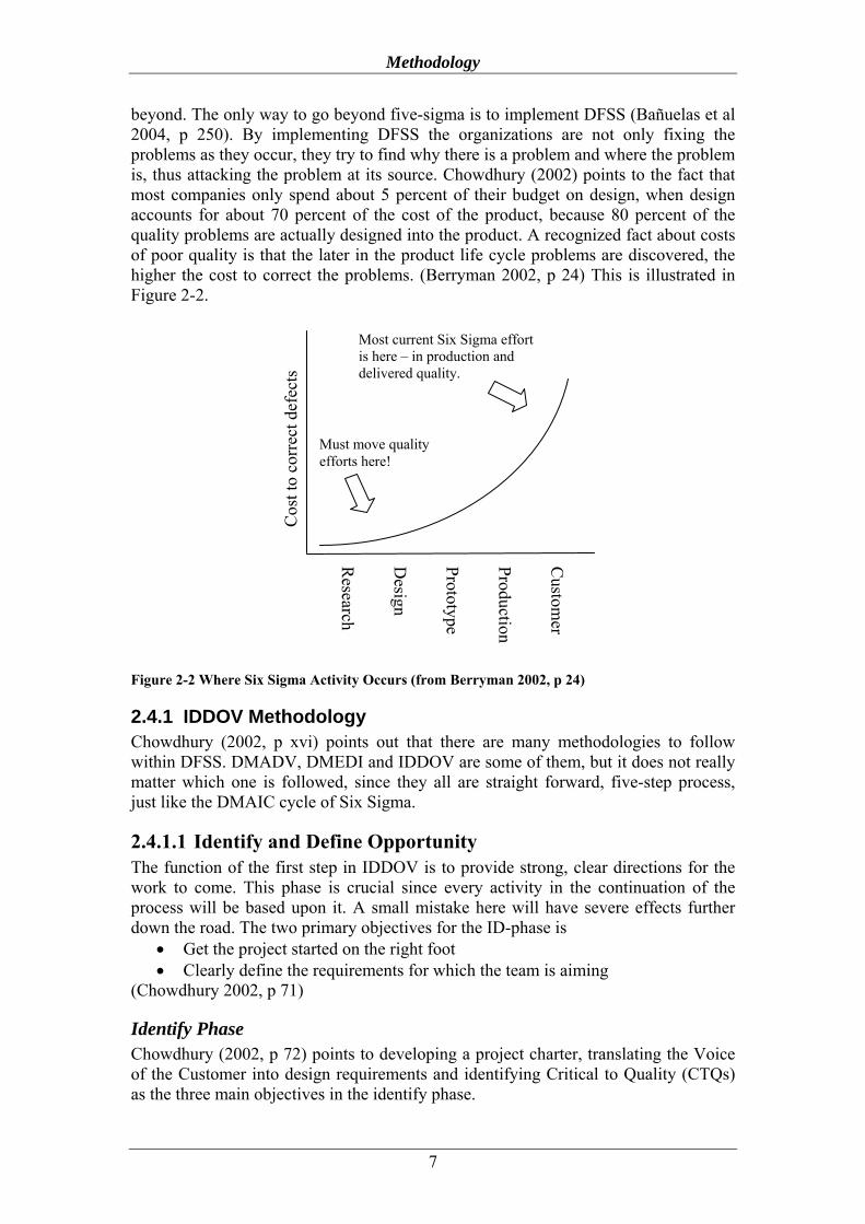
There are no points above or below the control limits, which indicates that the process is in control. The first point is however the same as the UCL. The capability indices for the vent are shown in Table 4-8.

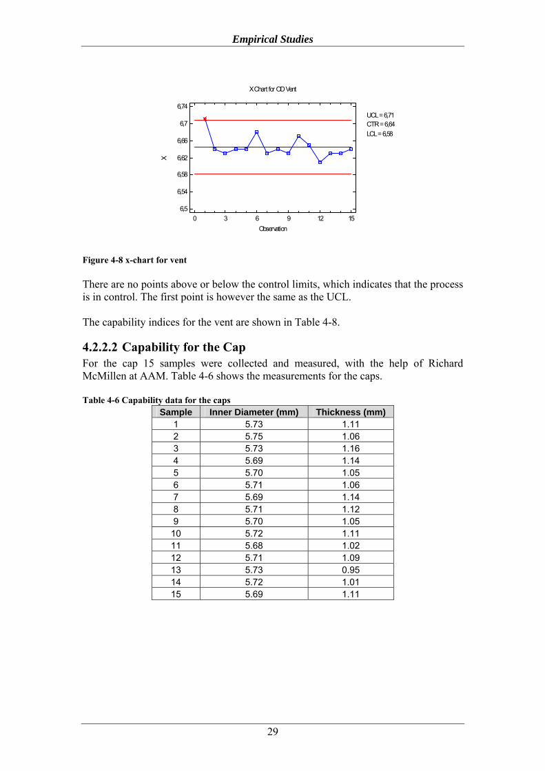
4.2.2.2 Capability for the Cap For the cap 15 samples were collected and measured, with the help of Richard McMillen at AAM. Table 4-6 shows the measurements for the caps. Table 4-6 Capability data for the caps

Sample Inner Diameter (mm) Thickness (mm) 1 5.73 1.11 2 5.75 1.06 3 5.73 1.16 4 5.69 1.14 5 5.70 1.05 6 5.71 1.06 7 5.69 1.14 8 5.71 1.12 9 5.70 1.05

10 5.72 1.11 11 5.68 1.02 12 5.71 1.09 13 5.73 0.95 14 5.72 1.01 15 5.69 1.11

X Chart for OD Vent

0 3 6 9 12 15Observation

6,5

6,54

6,58

6,62

6,66

6,7

6,74

X

CTR = 6,64UCL = 6,71

LCL = 6,58

Figure 4-8 x-chart for vent

Empirical Studies

30

To start off the capability study for the inner diameter a histogram and a normal distribution plot were made over the values. They, together with a Shapiro-Wilks test, show that it is not possible to reject the idea that the values come from a normal distribution, with a confidence of 99%. The histogram and normal probability plot are displayed as Figure A 11 in Appendix 6. Just as for the vents, the caps are distributed to AAM by a supplier, and arrive in large baskets of several hundreds. The same reasoning regarding the MR-chart is used here, as for the vents. Instead the x-chart is put up, Figure 4-9.

Figure 4-9 x-chart for inner diameter Also here, no points were found to be outside of the control limits, and the process is therefore said to be in statistical balance. The same process used for the Inner Diameter is repeated for the Thickness. Just as for the inner diameter, the thickness was found to be normally distributed with a confidence lever of 99%. The histogram and normal distribution plot are shown in Figure A 12. For the thickness, the x-chart is shown in Figure 4-10. Also for here the process is found to be in control.

Figure 4-10 x-chart for thickness

X Chart for ID Cap

0 3 6 9 12 15Observation

5,6

5,63

5,66

5,69

5,72

5,75

5,78

X

CTR = 5,71UCL = 5,77

LCL = 5,65

X Chart for Thickness cap

0 3 6 9 12 15Observation

0,89

0,99

1,09

1,19

1,29

X

CTR = 1,08UCL = 1,26

LCL = 0,90

Empirical Studies

31

The capability for inner diameter and thickness are shown in Table 4-8.

4.2.2.3 Capability for Lube weight The lube level filled was also found out to be interesting to investigate. At DGA the lube is filled at two different, but identical, stations since the filling is considered a bottle neck in the manufacturing process. At the two stations, named east and west, controls of the filling weight is made four times every day, from approximately 5 am to 8 pm.

East Side Station For the east side data from 10/27/05 until 12/06/05, a total of 83 samples were studied. Unfortunately the data between 11/18/2005 and 11/29/2005 was not collected and are thus not included in the study. First of all, a check for normality was done, Figure 4-11.

The normal probability test rejects the idea that the lube weight from the east side station comes from a normal distribution with 90% confidence. Since the values can not be looked upon as normally distributed, it complicates the interpreting of the capability study.

Quantile-Quantile Plot

1,6 1,64 1,68 1,72 1,76 1,8 1,84Normal distribution

1,6

1,64

1,68

1,72

1,76

1,8

1,84

Lube

wei

ght e

ast

DistributionNormal

Histogram for Lube weight east

1,6 1,65 1,7 1,75 1,8 1,85Lube weight east

0

10

20

30

40

50

frequ

ency

DistributionNormal

Figure 4-11 Histogram and normal distribution plot for lube weight east

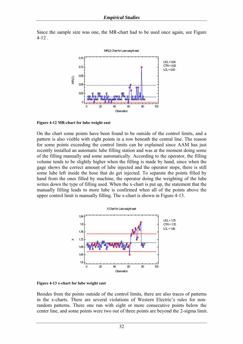
Empirical Studies

32

Since the sample size was one, the MR-chart had to be used once again, see Figure 4-12 .

Figure 4-12 MR-chart for lube weight east On the chart some points have been found to be outside of the control limits, and a pattern is also visible with eight points in a row beneath the central line. The reason for some points exceeding the control limits can be explained since AAM has just recently installed an automatic lube filling station and was at the moment doing some of the filling manually and some automatically. According to the operator, the filling volume tends to be slightly higher when the filling is made by hand, since when the gage shows the correct amount of lube injected and the operator stops, there is still some lube left inside the hose that do get injected. To separate the points filled by hand from the ones filled by machine, the operator doing the weighting of the lube writes down the type of filling used. When the x-chart is put up, the statement that the manually filling leads to more lube is confirmed when all of the points above the upper control limit is manually filling. The x-chart is shown in Figure 4-13.

Figure 4-13 x-chart for lube weight east Besides from the points outside of the control limits, there are also traces of patterns in the x-charts. There are several violations of Western Electric’s rules for non-random patterns. There one run with eight or more consecutive points below the center line, and some points were two out of three points are beyond the 2-sigma limit.

MR(2) Chart for Lube weight east

0 20 40 60 80 100Observation

0

0,03

0,06

0,09

0,12

0,15

MR

(2)

CTR = 0,02UCL = 0,06

LCL = 0,00

X Chart for Lube weight east

0 20 40 60 80 100Observation

1,6

1,64

1,68

1,72

1,76

1,8

1,84

X

CTR = 1,70UCL = 1,75

LCL = 1,66

Empirical Studies

33

West Side Station The same procedure is then repeated for the data from the west-side filling station. Here the samples are from 10/11/2005 to 12/6/2005, a total of 112 samples. Unfortunately samples between 10/17/2005-10/25/2005 and 11/27/2005-12/2/2005 are missing. The histogram and normal distribution plot is shown in Figure 4-14.

Just as for the east side, the normal probability test rejects the idea that the lube weight for the west side station comes from a normal distribution with 90% confidence. The study was continued with a MR-chart, Figure 4-15.

Histogram for Lube weight west

1,7 1,74 1,78 1,82 1,86 1,9Lube weight west

0

20

40

60

80fre

quen

cyDistribution

Normal

Quantile-Quantile Plot

1,7 1,73 1,76 1,79 1,82 1,85 1,88Normal distribution

1,7

1,73

1,76

1,79

1,82

1,85

1,88

Lube

wei

ght w

est

DistributionNormal

Figure 4-14 Histogram and normal distribution plot for lube weight west

Empirical Studies

34

Figure 4-15 MR-chart for lube weight west For the west-side there are not as many points outside of the control limits as for the east-side. For the MR-chart there are three points above the upper control limit and nine points in a row below the lower control limit. For the x-chart, Figure 4-16, there are some points above the upper control limit. There are also one set with eight consecutive points below the center line, and some sets were four out of five runs are outside of the 1-sigma limit and were two out of three runs are outside of the 2-sigma limit.

Figure 4-16 x-chart for lube weight west When the data from the two stations are compared to one another, the west-side station seems to have shifted away towards the upper specification limit if compared to the east-side. This is illustrated in Figure 4-17.

MR(2) Chart for Lube weight west

0 20 40 60 80 100 120Observation

0

0,02

0,04

0,06

0,08

0,1

MR

(2)

CTR = 0,02UCL = 0,05

LCL = 0,00

X Chart for Lube weight west

0 20 40 60 80 100 120Observation

1,7

1,73

1,76

1,79

1,82

1,85

1,88

X

CTR = 1,79UCL = 1,83

LCL = 1,74

Empirical Studies

35

Interesting to know is if the actual filling weight is different from the specified filling weight of 1.70 kg. With a significance level of 1% the hypotheses are

• H0 : μ = 1.7

• H1 : μ ≠ 1.7 Using the equations for σ* and t as presented in chapter 2.10, the results are as shown in Table 4-7. Table 4-7 Hypothesis test for filling stations

μ σ* x t k East 1.7 0.033 1.703 0.967 2.660 West 1.7 0.020 1.786 44.783 2.617

For the east side H0 is not rejected since t<k with 1% significance level. However for the west side H0 is rejected with a significance level of 1%, since t is considerably larger than k.

4.2.2.4 Capability Summary The capability for the vent, cap and lube weight are calculated using the equations in chapter 2.8.1. The values are presented in Table 4-8. Table 4-8 Capability indices

Cp Cpk Cpm

Vent Outer Diameter 3.37 2.09 1.70

Inner Diameter 0.86 0.85 0.86 Cap Thickness 2.91 2.45 1.71 West 3.54 2.70 0.81 Lube

Weight East 2.18 1.86 2.16 As shown in Table 4-8 the capability for the vent shows that the value for Cp is good. The slightly smaller value of Cpk shows that the caps are not very well within specification. The small Cpm indicates that there is a big deviation from the target

0

5

10

15

20

25

30

1.60

1.62

1.64

1.66

1.68

1.70

1.72

1.74

1.76

1.78

1.80

1.82

1.84

1.86

1.88

1.90

Lube weight (Kg)

WestEast

Figure 4-17 The distribution of west and east side filling stations

Empirical Studies

36

value, in this case the diameters are bigger than specified. But, since the process is not normal distributed or in statistical control the values carry less importance, than if the process would have been in control and normal distributed. However, if changes are made it is possible to tell if they have improved or worsen the process. The capability indices for the cap show that the inner diameter is not capable. Cp is very small, which indicates there is a big spread between the values. The fact that Cpk is almost as big as Cp, shows that the process is well within specifications, which is also strengthened by the Cpm value. The thickness on the other hand is better that the inner diameter, but not good enough. A Cp of 2.91 is not good enough. There is also a slight deviation from Cp in the Cpk, and the smaller Cpm show that the process has diverged from the target value. On the control charts in, Figure 4-9 and Figure 4-10 there are no points outside of the control limits, but since the data are not collected in a chronological order, it is not possible to determine with certainty if the process is in control. For that reason little emphasis is put on the capability values. The values for the capability for the west side station are pretty good. Cp is hight, but unfortunately Cpk is lower, which indicates that the process is not in midpoint of the specifications. This is also shown by a very small Cpm value. The low value of Cp for the east side shows that there is a bigger spread than for the west side. Cpk is also small which indicates that the process is incapable of filling axles well within specifications. The process is however well on target value. The difference between the two stations is shown in Figure 4-17. From the control charts in Figure 4-12 , Figure 4-13, Figure 4-15 and Figure 4-16 there is evidence that the process of filling the axles with lube is not in statistical control. Both stations have points outside the control limits. This might be because of the reason that some axles are still filled by hand, while others are filled automatically. But other than that, they also fall victim to Western Electric’s rules for non-random pattern, even for series of points all filled automatically. Since the process is not normal distributed or in statistical control the values capability study carries less importance, than if the process would have been in control and normal distributed. However, if changes are made it is possible to tell if they have improved or worsen the process. In Appendix 6, there are figures showing the process capability for the design study.

4.2.3 Component Search Since no direct conclusions could be drawn from the capability test, a component search was conducted to see where the problem lies. The response variable was decided to be at the amount of pressure it takes before air starts to sip out from the vent-cap area. To be able to see if there is any difference in the amount of air that escapes from the vent tube – cap area between different axles, data from the air leak test at DGA was collected and studied. In the air leak study the axles are pressurized to 7 psi and the air escaping from the axles must be between 800 and -150 ccm. Steve Wasik explained that the negative number originates from the fact that the axle is cold, and when warmer air is injected there is sometimes a vacuum created when the air cools down. When this occurs the axles do not leak out air, but actually take in air instead. Important to remember though is that the axles might leak from other areas than just the vent tube – cap area. The data collected from 12/19/2005 showed a range from 6787 ccm to -143. Axles that do not pass the air leak test will automatically run through the repair loop where the operator locates the leak and investigates if it is

Empirical Studies

37

repairable. According to the operator the majority of the time the leak is between the rear cap and the differential. This is usually caused by a broken bolt. In Table 4-9, the data over the air leak test from 12/19/2005 is displayed. From the air leak test, five really high numbers were noticed. They often appear when there is something major missing or leaking on the axles. For instance, sometimes the vent is not correctly installed and will pop off during the leak test. Since leaks like that are between the vent and differential and not vent and cap, the measurements from those axles were not considered interesting for the investigation. The chart on the right hand side in Table 4-9 displays the case when the five high ones have been excluded. Table 4-9 Data over the air leak test. In the right hand chart the five highest values have been excluded

Air Leak Test Air Leak Test Max 6787.00 Max 782.00 Min -143.00 Min -143.00 Range 6930.00 Range 925.00 Stnd dev 248.84 Stnd dev 162.01 Mean 171.55 Mean 163.62

From the run of 12/20/2005, data on a total of twelve axles was collected. The axles chosen were six with a leak as close to zero as possible, and six to be as high as possible. This was the BOBs and WOWs. The idea was to have as big of a contrast as possible between the two samples. When found, the axles were pulled off the line before they were filled with lube, to make it easier to pressurize and measure. At AAMs reliability center the axles were pressurized until they leaked around the vent – cap area. This was done by spraying a water and soap mix onto the area, and observe at what pressure the mix started to bubble. This way it was known that the leak was around the vent-cap area and not anywhere else. This was done three times to each axle, with a disassembly and reassembly of the cap between the runs, to make sure that any error in the assembling of the cap had as low impact as possible. The findings are displayed in Table 4-10. Originally eight axles of each kind were selected, but since the racks only have a six axle capacity, six were collected instead of eight. Table 4-10 Pressure Test

Original reading (ccm)

Run 1 (psi)

Run 2 (psi)

Run 3 (psi) Average Stndev Range

BOB2 5,70 11 6 3 6.67 4.04 8 BOB3 2,75 17 5 5 9.00 6.93 12 BOB4 1,53 14 7 9 9.83 3.33 7 BOB5 4,68 12 7 10 9.67 2.52 5 BOB6 0,61 15 15 16 15.33 0.58 1 BOB8 5,60 19 18 10 15.67 4.93 9 11.03 3.72 6.92 WOW1 720,41 5 3 3 3.67 1.15 2 WOW3 375,28 11 2 5 5.67 4.86 10 WOW4 324,98 8 3 3 4.50 3.04 6 WOW5 491,65 3 3 2 2.67 0.58 1 WOW6 365,91 11 13 8 10.67 2.52 5 WOW7 387,85 6 13 11 9.67 3.82 8 6.14 2.66 5.08

Empirical Studies

38

After the first runs of the axles the caps were switched between the axles. The idea was yet again to create as big contrast as possible. The data of the findings are presented in Table 4-11 and in Figure 4-18 is a chart over the data. Table 4-11 Switching caps between high and low leakers

R 1 (psi)

R 2 (psi)

R 3 (psi) Average Stndev Range

Cap Axle BOB2 WOW6 3 3 3 3.0 0.0 0.0 BOB3 WOW7 5 4 2 3.7 1.5 3.0 BOB4 WOW3 6 8 5 6.3 1.5 3.0 BOB5 WOW4 8 7 5 6.7 1.5 3.0 BOB6 WOW1 2 2 1 1.7 0.6 1.0 BOB8 WOW5 2 2 3 2.3 0.6 1.0 Cap Axle WOW6 BOB2 5 4 5 4.7 0.6 1.0 WOW7 BOB3 2 1 1 1.3 0.6 1.0 WOW3 BOB4 8 8 6 7.3 1.2 2.0 WOW4 BOB5 6 4 4 4.7 1.2 2.0 WOW1 BOB6 2 3 1 2.0 1.0 2.0 WOW5 BOB8 10 9 14 11.0 2.6 5.0

The first six observations are plotted in Figure 4-18 with the BOBs on top and the WOWs in the bottom. Although the Component Search does not seem to pass the two rules of the Component Search, as described in chapter 2.9.4, the search was continued. Mainly to see if there was a pattern or any clues that would help in the next parts of the project. The caps from the BOB axles are put on the WOW axles, and the caps from the WOW axles on the BOB axles. If the issue would reside solely within the cap or vent, this would have been visible in the graph as a gap between the two lines. But, in this case the two lines are too close to one another, and no conclusions can be drawn from the Component Search. The reason for the plots being so close to each other can be many. One cause might be that the issue does not lay in the cap or the vent itself, instead it is an interaction between the two of them, or the reason some axles leak have nothing at all to do with the vents or caps. Another cause might be that the cap wears out after being pulled a couple of times, so that measuring becomes

0.0

2.0

4.0

6.0

8.0

10.0

12.0

14.0

16.0

18.0

1 2 3 4 5 6 7 8 9 10 11 12

Pres

sure

(psi

)

Figure 4-18 Outcome of Component Search

Empirical Studies

39

more and more inaccurate. To see if the cap wears out as a result of pushing it on and pulling it off, five randomly selected caps were taken and pressure tested onto a vent. The pressure was isolated onto the cap itself, and the amount of pressure needed to pop the caps was observed. The findings are shown in Table 4-12. Table 4-12 Cap wear-out test

Cap 1 2 3 4 5 Average (psi)

1 43 40 44 42 42 42 2 40 38 40 39 40 39 3 38 36 39 38 38 38 4 38 36 38 38 37 37 5 38 36 37 37 37 37 6 36 36 36 37 37 36 7 37 36 37 37 37 37 8 37 35 37 37 37 37 9 37 35 36 37 37 36

10 37 35 36 36 37 36 11 39 36 40 39 38 38 12 37 35 37 37 37 37 13 37 36 38 38 40 38

Run

14 37 35 37 37 39 37 From run 1 to 10 all ten runs were done with no break between the runs. To see if the cap retains some of its strength after a break, a shorter break was held between run 10 and 11. An even longer one was held between run 12 and 13. Table 4-12 clearly shows that the cap does get lose after being pulled a couple of times. The rate of decay is more clearly shown in Figure 4-19.

Even though the caps do get worn out from being pulled off, it is only a couple of percent in decay between the different runs. Even with this decay in mind, it does not make any difference for the component search, since they amount of pressure is very low and a few percentages more or less will not make any significant difference.

34

36

38

40

42

44

1 2 3 4 5 6 7 8 9 10 11 12 13 14

Pres

sure

(psi

)

Figure 4-19 The wear out of the cap

Empirical Studies

40

From the values of the capability test and from the component search it is hard to draw any conclusions. The only conclusions that can be drawn from the capability test are conclusions from an increase or a decrease of the capability indices, from one test to another. Although it is hard to draw conclusions from the study, neither one of the vent, cap or lube weight is thought of as a likely single-handed contributor to the problem. This is based upon, besides the study, discussions with people from AAM and GM, well familiar with the problem and process. Instead, the most interesting finding from this phase was the extra task of switching caps at GGA and Three Rivers, which were not a part of the process at DGA. But, for that reason, there is no proof saying that either one of the vent, cap or lube weight might interact with the pressure to cause leak.

4.2.4 Operations Search Since pressure is the most likely driver of the issue, the next step is to decide where in the process the pressure is built up. Normally this is done by using an Operations Search Diagram, but since it was very hard to have a look at every step inside the process to determine exactly when the axles start to leak, another approach had to be used. Since before, axles being wet had been noticed when leaving PTI, but never when arriving. After discussion with Mike Palecek, Steve Wasik and Dolores Alcantar (Quality Manager at PTI), the conclusion was that the only phase where pressure could be built up at PTI was inside the oven where the axles are dried, see Figure A 3.

4.3 Optimize the Design From the investigations in Identify and Define and Develop Concepts, pressure created from the heat applied to the axles when drying the paint was found to be the most likely driver of the leaks. From the pop-off test the amount of pressure to pop the cap off was found to be very high, significantly higher than what the axle is put through from normal use. So the question of heat resistance for the cap and vent quickly rose.

4.3.1 Design of Experiments To see how the cap and vent react to heat, a heat study was made. AAM had only an oven that could reach 360º F, and not one that could be put to 200º F. For the initial research the AAM oven had to be used. A total of 15 pairs of vent-caps were collected and measured initially. The measurements are presented in Table 4-13.

Empirical Studies

41

Table 4-13 Vents and caps for heat study VENT CAP

Sample Outer Diameter (mm) Sample Inner Diameter

(mm) Wall Thickness

(mm) 1 6.71 1 5.73 1.11 2 6.64 2 5.75 1.06 3 6.63 3 5.73 1.16 4 6.64 4 5.69 1.14 5 6.64 5 5.7 1.05 6 6.68 6 5.71 1.06 7 6.63 7 5.69 1.14 8 6.64 8 5.71 1.12 9 6.63 9 5.7 1.05

10 6.67 10 5.72 1.11 11 6.65 11 5.68 1.02 12 6.61 12 5.71 1.09 13 6.63 13 5.73 0.95 14 6.63 14 5.72 1.01 15 6.64 15 5.69 1.11

At first, the biggest and smallest outer diameter of the vent was taken as research vents. This was to create as big contrast as possible. After that each of the two vents were connected to an air pressured hose. All of the 15 caps were put on in random order and pressurized until the cap popped off the vent. This was done twice for each cap so a mean could be calculated. Table 4-14 shows the pop-off pressure required before the cap and vents were heated. Table 4-14 Pop-off test before heating

Vent 1 Run psi Run psi Mean Stndev Cap 1 15 44 22 42 43.0 1.4 Cap 2 1 39 28 42 40.5 2.1 Cap 3 12 45 18 44 44.5 0.7 Cap 4 4 41 21 41 41.0 0.0 Cap 5 5 40 26 41 40.5 0.7 Cap 6 11 40 17 42 41.0 1.4 Cap 7 14 45 24 44 44.5 0.7 Cap 8 13 43 27 42 42.5 0.7 Cap 9 7 42 29 45 43.5 2.1 Cap 10 3 42 20 44 43.0 1.4 Cap 11 8 42 30 44 43.0 1.4 Cap 12 6 42 16 44 43.0 1.4 Cap 13 9 42 19 43 42.5 0.7 Cap 14 2 42 23 44 43.0 1.4 Cap 15 10 44 25 42 43.0 1.4 42.2 42.9 42.6 1.2

Empirical Studies

42

Vent 12

Run psi Run psi Mean Stndev Cap 1 5 39 20 41 40.0 1.4 Cap 2 8 40 28 39 39.5 0.7 Cap 3 3 41 18 42 41.5 0.7 Cap 4 14 40 23 40 40.0 0.0 Cap 5 9 40 24 39 39.5 0.7 Cap 6 7 41 29 42 41.5 0.7 Cap 7 1 40 22 40 40.0 0.0 Cap 8 4 39 17 40 39.5 0.7 Cap 9 15 41 26 42 41.5 0.7 Cap 10 13 41 19 41 41.0 0.0 Cap 11 11 42 25 41 41.5 0.7 Cap 12 6 41 16 40 40.5 0.7 Cap 13 10 41 27 41 41.0 0.0 Cap 14 12 41 30 41 41.0 0.0 Cap 15 2 40 21 42 41.0 1.4 40.5 40.7 40.6 0.6

After the initial pop-off test the caps were heated in 360º F for 15 minutes. Unfortunately, the box the vent-cap pairs were put into did not withstand such a high heat, leading to the loss of four pairs left in the remains of the box. Luckily the two important vents used in the first test survived the oven. After the heating, a pop-off test just like the first one was carried out. Table 4-15 shows the pop-off pressure after the cap-vent pairs have been in the oven. Table 4-15 Pop-off test after heating

Vent 1 Run psi Run psi Mean Stndev Cap 1 1 13 18 14 13.5 0.7 Cap 2 8 19 20 20 19.5 0.7 Cap 3 Cap 4 3 17 12 15 16.0 1.4 Cap 5 11 20 13 18 19.0 1.4 Cap 6 Cap 7 2 20 15 21 20.5 0.7 Cap 8 7 19 22 18 18.5 0.7 Cap 9 5 21 16 20 20.5 0.7 Cap 10 6 15 19 15 15.0 0.0 Cap 11 Cap 12 9 21 21 20 20.5 0.7 Cap 13 10 20 14 20 20.0 0.0 Cap 14 Cap 15 4 21 17 21 21.0 0 18.7 18.4 18.5 0.6

Empirical Studies

43

Vent 12

Run psi Run psi Mean Stndev Cap 1 8 13 22 13 13.0 0.0 Cap 2 10 18 15 16 17.0 1.4 Cap 3 Cap 4 7 16 19 15 15.5 0.7 Cap 5 9 18 14 17 17.5 0.7 Cap 6 Cap 7 6 20 21 20 20.0 0.0 Cap 8 3 16 20 16 16.0 0.0 Cap 9 5 19 16 18 18.5 0.7 Cap 10 4 14 17 15 14.0 0.0 Cap 11 Cap 12 2 19 18 20 19.5 0.7 Cap 13 1 17 12 19 18.0 1.4 Cap 14 Cap 15 11 20 13 18 19.0 1.4 17.3 16.9 17.1 0.6

As shown in Table 4-14 and Table 4-15, there is a difference in the pop-off pressure required between both the max and min vent as well as before and after the caps been heated. Table 4-16 is a summary over the mean and standard deviation for the pop-off pressure. Table 4-16 Summary of the pop-off pressure

Before heating After heating Vent 1 Vent 12 Vent 1 Vent 12 Mean 42.6 40.6 18.5 17.1 Stndev 1.2 0.6 0.6 0.6

Important to remember though is the fact that the cap does get worn out after being pulled too many times, as Figure 4-19 displays, so the actual difference might be slightly smaller than what Table 4-16 shows. When heat now has been proven to impact the characteristics of the yellow cap, a more specific connection would be interesting to find.

4.3.1.1 Factorial Design The three variables that were interesting to look further into was the vent diameter, time in the oven, and oven temperature. The vent diameter was hard to have full control over, so instead of using a normal variable measurement, an attribute measurement was used. The factorial design was decided to be a 23-1 design, with two replicates. Four center points were also created to investigate if there is any curvature in the response. As response the pop off pressure needed to pop off the cap was selected. The factor levels were selected as Table 4-17 shows.

Empirical Studies

44

Table 4-17 Factor levels Low High Vent (A) Small Large Temperature (B) 80º C 100º C Time (C) 3 min 7 min

Since the oven that would be used for the experiment used Celsius and not Fahrenheit, the original temperature of 200º Fahrenheit had to be converted into Celsius. To make things easier, the value was rounded off. The design with the response is shown in Table 4-18. Table 4-18 The design with response

Std run Vent OD Temp Time Vent Response (bar)

3 1 Large 80 3 1:1 4.025 9 2 Small 90 5 1:2 3.95 8 3 Large 100 7 1:3 3.55

11 4 Small 90 5 1:4 3.95 10 5 Large 90 5 1:5 3.925 5 6 Small 100 3 1:6 3.9 2 7 Small 80 7 1:7 3.85

12 8 Large 90 5 1:8 3.9 1 9 Small 80 7 1:9 3.85 6 10 Small 100 3 1:10 3.85 7 11 Large 100 7 2:1 3.85 4 12 Large 80 3 2:2 3.95

When looking at the half-normal plot, Figure A 18 in Appendix 7, factors B and C fall out as active effects. Important to remember though, is that since it is a 23-1 design, the main effects are aliased with two-factor interactions. In this case A is aliased with BC, B is aliased with AC, and C is aliased with AB. In other words, it is possible that instead of B and C being active factors, it might be the two-factor interactions AC and AB that are active. But, since A is not an active factor by itself, and the fact that interactions are not as likely to be active as a single factor, the active factors in this case are most likely B and C, as the half-normal plot shows. Also in the ANOVA table, Table A 4 in Appendix 7, the two factors can be pointed out as active. The table also shows that there is no significant curvature, and the model is therefore linear. The final equation for the model is; Pop-off pressure = 4.63906 - 6.56250E-003 * Temp - 0.039062 * Time From the equation it is clear that temperature and time both contribute to a lower pop-off force. In other words, the higher temperature and/or longer time, the lower pressure is needed to pop the cap off from the vent. This is also shown in Figure A 19 and Figure A 20 in Appendix 7. The experiments left the caps more or less damaged. Figure 4-20 shows the difference between three caps. The first cap has been heated to 90ºC and the third one to 360ºF, and the cap in the middle has not been treated by any heat at all. When examining the base of the caps, it is clear that they differ between the three caps. The caps that have been exposed to heat appear to be deformed, and have started to take the shape of the

Empirical Studies

45

vent. The deform seems to be greater for cap 3, that has been exposed to a higher temperature than cap 1.

4.3.2 Process Improvement Most clues point to the fact that the yellow cap is not able to sustain the amount of pressure that is built up in the differential during the manufacturing process. There is most likely a number of less complicated ways to resolve this problem. The simplest one is likely to just pull the cap off after the paint process and let the pressure equalize before putting it back on again. With the latest part of knowledge of the process, the last section of the Project Definition Tree that displays the root cause of the issue can be created. The last part is presented in Figure A 7 in Appendix 3.

4.4 Verify the Design The solution of the leaking rear axles’ problem was to pull the yellow cap off after the paint process. This way the pressure created inside the differential during the time in the oven will be equalized and the cap will not be subject to as high of force. Since the middle of November 2005 the task of removing the cap for about five seconds has been added to the process at PTI, as shown in Figure A 21 in Appendix 8. As a part of GMs confirmation process, a Binomial Probability test was carried out with the help of Glen Pruden (Statistical Engineer), as shown in Figure A 22 in Appendix 9. Since the change in the process, a continuous communication with AAM, PTI and GMs assembly plants have been held to keep track of any upcoming issues with leaks around the vent tube and cap area. So far no leakers have been reported from any of the assembly plants or from PTI. In Appendix 10, there is a more detailed description of the process changes, made by Steve Wasik.

1 2 3

Figure 4-20 Cap 1 heated to 90ºC, cap 2 to not heated, and cap 3 heated to 360ºF

Conclusions

46

5 Conclusions This chapter is highlighting the results of the project, the conclusions drawn from it, and the suggested change in the process. The estimated savings as a result of this project is also presented in this chapter. The problem for this project was that some of the 8.6” rear axles for General Motors GMT900 program were found to be leaking during manufacturing and assembling process. Some axles with fluid on the differential or cover pan had also been found by customers from time to time. The problem area had been located and narrowed down to a vent located on the differential. The purposes for the project was to find out why some axles leak, while others do not and to suggest a process or design change in order to reduce or eliminate the number of leaking axles. It is no doubt that the concern with leaking rear axles has been drastically reduced since the suggested process change. Although it is hard to fully estimate the full extent of the leaking axles issue before the change in process, it is clear that it has not been any reports or observations of any leaking axles since the change. The reason for it being so hard to estimate the full extent is because some leaking axles make it all the way to the customer without ever being spotted, and some axles are covered with fluid because an axle above it has been leaking during transportation. Also, many axles with fluid that were spotted during assembling were just wiped off and examined to make sure they were not leaking anymore, before being put back out in production. This way the proper documentation of the leaking axles were never made. In the design study of the project a closer inspection of the vent, cap and lube was made. Although all three of them showed areas of potential major improvements, none of them were thought to be single handedly driving any axles to leak. Instead it is in the process study the cause and solution to the problem lies. The most likely driver of the leaks was found to be pressure built up inside the differential. Pressure is built up inside the differential when the axles go through a 200º F oven for about five minutes. From the heat inside the oven, the cap gets deformed, which probably also contributes to the leaks. When the paint has been dried the axles are, after some additional work, placed in racks before being shipped off. From this point and onwards in the process, leaking axles has been found. In some cases lube squirts out when the cap is pulled and replaced by the hose, and in other cases lube is pressed out of the vent, when the cap has been weakened by the heat. Most of the time, the pressure is only experienced as a puff of air, occasionally with a silent hissing sound, expelling from the axle when the cap is pulled. The solution and answers to the purposes of the project are;

• Some axles leak because of an increase of pressure inside the axle, created during the paint drying process inside the oven. The pressure is never equalized and for some axles the lube is pressed out from the vent.

• The number of leaking axles has been drastically reduced after a change in the process. A new task of pulling the caps, and by that also equalizing the pressure, has been added as an extra task after the axles have been in the oven.

Conclusions

47

5.1 Suggestions To eliminate the issue of the leaking axles, the suggestion is to continue with the extra added task of pulling the cap at PTI, as described in Appendix 10. Preferably, a new cap is to be used instead of the old and used one, since the old cap has been deformed from the heat in the oven and a fresh yellow cap indicates that the axle has been pressure equalized. By doing that the chance of mixing equalized and non-equalized axles is eliminated. In addition to that, some attention could be put on the capability of the vent, cap and lube weight. A more thoroughly capability study on the three of them would be a good thing to make. New machinery and manual filling might be the big reason behind the relatively poor capability for the lube weight. In this case the filling weight was more than specified, and if that is reduced, additional money could be saved with a filling process closer to target and with smaller variance.

5.2 Costs and savings The task of pulling the caps after the paint process is a cheap solution to the problem. There are a lot of operators in contact with the axles after they have been in the oven, so the current workforce should be sufficient to carry out the extra task added. According to Table A 1 in Appendix 4 the total yearly cost of leaking axles is approximately $ 58,500. As earlier mentioned these numbers do not give any exact value of the extent of the problem. According to Supplier Quality and Launch Manager Jim Pastor, a reasonable estimation would be around 50% of that value, or about $ 29,000.

Discussion

48

6 Discussion This chapter is a discussion of the results and of the chosen methodology and execution of the project. A short discussion of the reliability and validity is presented, and in the end suggestions for continuation of the problem. Although most clues point to the pressure as the cause of the issue, it is not certain that the pressure built up is the only contributor. This is mainly because of the lack of leaking axles to investigate. Other feasible causes might be the filling volume for each axle or the characteristics of the cap or the vent. Each one might be a cause by itself, or it might also be an interaction between them. As proved earlier the filling volume does differ between the two stations, and it is feasible that the axles that do leak come from the West side filling station that fills with a larger amount of lube than intended. At en inspection of the lube level of an axle, the lube level is found to be about ¾” below the vent, when the axle is in vertical position. A small distance like this is easily disturbed by a tilt in the axle position, and when it is lube will seep into the vent. Or perhaps have the caps on the leaking axles for some reason been less tolerant to heat than the caps on the non-leaking axles. One of the biggest problems when trying to solve the issue of leaking axles has been the lack of leaking axles to investigate. There are several reasons for this. One of the bigger ones is that the plants where the leaking axles normally are found are spread across the US and Canada and are thus hard to get to. For places nearby, like PTI, the axles are kept in large racks, piled high and close to one another. Even if there were any axles leaking, the chance of finding them was very small. That combined with the fact that the project was carried out during the launch of the GMT900 which means there was limited time to look for leaking axles to be pulled off of the line. Yet another reason is a miscommunication with AAM who early in the project made some changes in their process to eliminate or reduce the number of leaking axles. This means that the number of leaking axles where drastically reduced even in the early stages of the project. To make sure that the project worked from a basis with as accurate facts as possible, a number of field trips where made to AAM and their supplier PTI as well as to different assembly plants. During all of the trips there were people from AAM and/or GM present to explain the process and to answer any questions that were raised during the visit. Before making any decisions there was most of the time a discussion with supervisor Jim Pastor and occasionally also with the supervisor from the university, Rickard Garvare, to make sure the reliability was as good as possible. The accuracy of the gauges and the huge variety from cap to cap decreases the reliability and validity of the project. To make up for this all measuring has been made at least twice to get an average result. When measuring the pop-off force a camera has recorded the gauge, to get as accurate readings as possible in order to get a higher reliability. The reliability has probably suffered in the pop-off force since there was no easy way to control the amount of air inserted. Instead the device was controlled by pressing a handle, which is hard to exactly press equally as hard every time. As mentioned above, all decisions regarding methodology has been made after consulting with Jim or Rickard, to ensure a high degree of reliability and validity.

Discussion

49

The improvements made are however unquestionable. Since the change in the process, no leaking axles has been spotted or reported. For General Motors this means saving of about $ 29,000 annually, for the 8.6” axle alone. Since the task of pulling the cap is an easy and quick solution to the problem, it does not need any investments and is not the cause of any extra costs. A subject for deeper research within this area would be to look into the specifications of the plastic cap. Since the cap is in one way or another deformed in the oven, the original characteristics are changed. Therefore it might be possible to change the dimensions of the cap. Another thing to look into is the characteristics of the plastic itself. There might be some way to make the plastic more tolerant to heat, or maybe a way to let it expel air without letting any lube to escape from the axle.

References

50

7 References

7.1 Printed Sources Bañuelas R. and Antony J. (2004) Six Sigma or design for six sigma. The TQM Magazine. Vol. 16 No. 4, pp 250-263 Bell J. (2000) Introduktion till forskningsmetodik. Studentlitteratur, Lund Sweden. ISBN 91-44-01395-7 Bergman B. and Klefsjö B. (2001) Kvalitet från behov till användning. Studentlitteratur, Lund Sweden. ISBN 91-44-01917-3 Bergman B. and Klefsjö B. (2003) Quality from Customer Needs to Customer Satisfaction. Studentlitteratur, Lund Sweden. ISBN 91-44-04166-7 Berryman M.L. (2002) DFSS and Big Payoffs. Six Sigma Forum Magazine Vol. 2 No. 1, pp 23-28. Caulcutt R. (2001) Why is Six Sigma so Successful? Journal of Applied Statistics. Vol. 28 Nos. 3&4, pp 301-306 Chowdhury S. (2002) Design for Six Sigma: The Revolutionary Strategy for Achieving Extraordinary Profits. Dearborn Trade, Chicago, USA ISBN 07-93-15224-0 Creveling C.M., Slutsky J.L. and Antis D. (2003) Design for Six Sigma – In Technology and Product Development. Prentice Hall, New Jersey, USA. ISBN 0-13-0092231 Hoerl R.W. (2002) An Inside View of GE’s Six Sigma Experiences. GE Global Research. April 2002. Johnson L.T. and Tisell J. (1989) En dugligare tillverkning. Studentlitteratur, Lund Sweden. ISBN 91-44-30551-6. Magnusson K., Kroslid D. and Bergman B. (2003) Six Sigma the Pragmatic Approach, Studentlitteratur, Lund, Sweden. ISBN 91-44-02803-2 Montgomery D.C. (2001) Design and Analysis of Experiments. John Wiley & Sons, Inc., New York, USA. ISBN 0-471-31649-0 Vännman K. (2002) Matematisk Statistik. Studentlitteratur, Lund Sweden. ISBN 91-44-01690-5

7.2 Internet Sources American Axle & Manufacturing – About us - Company Profile. Retrieved October 25th from http://www.aam.com/about/about_profile.html

References

51

General Electric (No Date) What Is Six Sigma? - The Roadmap to Customer Impact. Retrieved October 28th 2005 from http://www.ge.com/sixsigma/sixsigma.pdf General Motors – Corporate Info – History. Retrieved October 25th from http://www.gm.com/company/corp_info/history/ iSixSigma (No Date) The History of Six Sigma. Retrieved October 25th 2005 from http://www.isixsigma.com/library/content/c020815a.asp VisitDetroit – Detroit History. Retrieved December 5th from http://www.visitdetroit.com/visitorcenter/aboutdetroit/history/ VisitDetroit – Fun Facts About Detroit. Retrieved December 5th from http://www.visitdetroit.com/visitorcenter/aboutdetroit/funfacts/ Waxer, C. (No Date) Six Sigma Costs And Saving – The financial benefits of implementing Six Sigma at your company can be significant. Retrieved October 25th 2005 from http://www.isixsigma.com/library/content/c020729a.asp Wikipedia – The Free Encyclopedia. November 9th 2005 http://www.wikipedia.org Woodford D. (No Date) Design for Six Sigma – IDOV Methodology. Retrieved September 7th 2005 from http://www.isixsigma.com/library/content/c020819a.asp

7.3 Internal Documents GM University – Quality College Statistical Engineering Introduction 8-9-05 (GM2005) GM University – Quality College Statistical Engineering – Awareness 01-23-04 (Gm2004)

Appendix 1 – Flow charts

Gears put onto sled

Carrier with ringbolts, pinion flange, race, and bearings placed

onto sled

Ringbolts put onto ring gear

Pinion shim check

Pinion shim placed

Bearings pressed on

Flipped up-side down (pinion up)

Pinion flange installed

Fasten pinion bolt

Rotate pinion to check run

out and torque

Flipped back to pinion

pointed down

Air leak test300 cc and

7 psi

Gears into differential

shell

Side shim distance checked

Shims placed

Pressed together

Bearing caps installed

Rouge and patterns check

Stored

Figure A 1Flow chart for manufacturing the differential

Tubes washed an

pressed onto differential

Tubes are spot welded

Middle storage

Tone ring placed at the end of each

tube

Dust shields installed

Speed sensor cable

installed

Shafts installed

Vent plugs air pressured

onto differential

Split line east/west

Yellow cap placed onto

vent

Cover pan installed (3

bolts manually, rest automatically)

Speed sensor test

Air leak test at 800 ccm

Rotor or drum brakes

installed on calibers

Repaired

OK?

Axles are tagged with

specific number

Oil fill Axle plugged at cover OK?

Racked according to prefix code

Shipped to PTI

Taken off for destruction

Yes

Yes

Repaired

OK?

OK?

Yes

No

No

Yes

No

No

Figure A 2 Flow chart for manufacturing the rear axle

Axles are received

from DGAScanned

Placed in raw material to be

painted

Axles are washed at 150-170º F

Axles are blow-dried at 35 psi

MaskedAxles go

through flash tunnel

Axles go into oven at 200º F

Unloaded

Tagged depending on

defect

Are the axles ok?

Yes

Axles unloaded

Axles are painted at

20 psi

De-masked Stored Loads pulled

Pulled to dock

Taken to sorting area if

needed

Loaded to sequencer

Sent back to AAM

Are the axles ok?

Yes

No

NoPTI defect?

Repaired

No

Yes

Figure A 3 Flow chart at PTI

Axles are received from DGA or GGA

Axles are stored

Axles are put onto special sequence

racks

Additional work is

carried out

Axles are stored for a short while

Axles are shipped to

plant

Axles are received from

DGA

Axles are stored

Axles are stored for a short while

Axles are put onto special sequence

racks

Axles are shipped to

plant

Figure A 4 Flow chart for Arlington and Pontiac

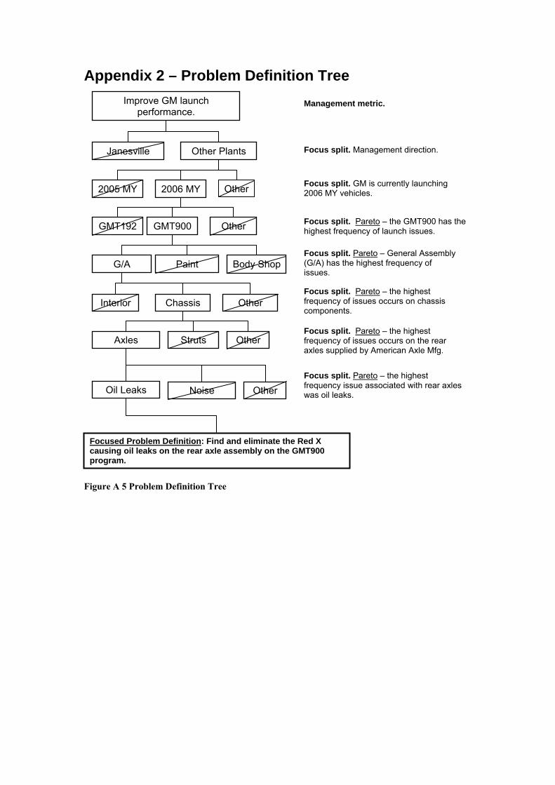
Appendix 2 – Problem Definition Tree Improve GM launch

performance.

Janesville Focus split. Management direction.

Focus split. Pareto – General Assembly (G/A) has the highest frequency of issues.

GMT192 Focus split. Pareto – the GMT900 has the highest frequency of launch issues.

Focused Problem Definition: Find and eliminate the Red X causing oil leaks on the rear axle assembly on the GMT900 program.

Management metric.

GMT900

Other Plants

2005 MY 2006 MY Focus split. GM is currently launching 2006 MY vehicles.

Other

Chassis Interior Focus split. Pareto – the highest frequency of issues occurs on chassis components.

G/A Paint Body Shop

Axles Other Struts Focus split. Pareto – the highest frequency of issues occurs on the rear axles supplied by American Axle Mfg.

Oil Leaks Other Noise Focus split. Pareto – the highest frequency issue associated with rear axles was oil leaks.

Other

Other

Figure A 5 Problem Definition Tree

Appendix 3 – Project Definition Tree

Figure A 6 Project Definition Tree

Rationale:

Focus split. The issue is an event (leak). Event Defect Feature

Dictionary split. Concentration Diagram – 90% of the leaks occur at the vent tube to cap interface (see Figure 4-2).

Strategy split. A part to part strategy was selected based on good contrast and leverage (see Table 4-2).

Focus split. Concentration Diagram – the leak occurs at the vent tube (see Figure 4-1).

OtherMain Gasket Vent Tube

Vent Tube to Housing Interface

Continued

Focused Problem Definition: Find and eliminate the Red X causing oil leaks on the rear axle assembly on the GMT900 program.

Vent Tube to Cap Interface

Variable Meas. Attribute Meas.

Part to Part Strategy Other

Focus Split. The issue is being evaluated on an attribute basis (leak/no leak).

Dictionary Split. Operation Search – No oil leaks viewed in process prior to the paint oven operation. Leaks were only observed after the paint oven operation, see Operations Search page 41.

Before Paint Oven After Paint Oven

Focus split. Process Flow Review – Parts are heated to 200 F after paint to insure proper paint cure. This is the highest source of energy into the system, see Figure A 3.

Other Temperature

Figure A 7 Project Definition Tree (Cont.)

Confirmation. Binomial Probability –58 parts were tested using the Bassembly process (vent cap removedafter paint oven) resulting in nofailures. Therefore, the new process isbetter than the old process with 95%confidence (see Figure A 22).

Failed to Prove Proved

Corrective Action. De-pressurize axle after paint oven operation by removing temporary yellow valve cap. Standard Operating Procedures have been updated to include this process step and a P-chart implemented at Janesville Assembly has verified effectiveness of the change. Note: This is a temporary cap that is removed at the vehicle assembly plant when the vent connector is attached.

Red X Candidate

Dictionary Split. Physics – Oil leak can only occur if internal pressure is greater than ambient. Heating enclosed volume of oil results in increased internal pressure. Process Flow Review - Active leaks only observed on heated parts from oven. Finished goods inventory parts with evidence of leak were wiped with no further evidence of active leaks.

Other Increased Internal Pressure

Appendix 4 – Early mileage divided up in plants Table A 1 Labor codes F2003 and F2023

Flint Pontiac Silao Arlington Oshawa Janesville Fort Wayne Vehicles 11,706 62,971 172,225 167,176 300,257 154,285 243,066Avg Exp 150.4 154.5 130.5 142.8 152.3 141.5 151.6Cases 35 40 89 74 136 58 88IPTV 3.58 0.74 0.71 0.56 0.54 0.48 0.43CPV ($) 0.44 0.07 0.09 0.06 0.06 0.05 0.05 Total Cost ($) 4,288.42 3,919.05 10,970.08 8,380.91 14,867.51 6,412.82 9,575.52

Table A 2 Labor code F2023 (Seal, pinion shaft oil)

Flint Pontiac Silao Arlington Oshawa Janesville Fort Wayne Vehicles 11,706 62,971 172,225 167,176 300,257 154,285 243,066Avg Exp 150.4 154.5 130.5 142.8 152.3 141.5 151.6Cases 32 18 64 41 70 33 45IPTV 3.27 0.33 0.51 0.31 0.28 0.27 0.22CPV ($) 0.41 0.04 0.07 0.04 0.04 0.04 0.03 Total Cost ($) 4,029.71 2,323.16 9,116.17 5,777.25 9,719.88 4,275.33 6,477.47

Table A 3 Labor code F2003 (Cover and/or gasket differential)

Flint Pontiac Silao Arlington Oshawa Janesville Fort WayneVehicles 11,706 62,971 172,225 167,176 300,257 154,285 243,066Avg Exp 150.4 154.5 130.5 142.8 152.3 141.5 151.6Cases 3 22 25 33 66 25 43IPTV 0.31 0.41 0.20 0.25 0.26 0.21 0.21CPV ($) 0.03 0.03 0.01 0.02 0.02 0.02 0.02 Total Cost ($) 258.71 1,595.89 1,853.91 2,603.66 5,147.63 2,137.49 3,098.05

Appendix 5 – Transportation

Figure A 8 Axles at PTI before they are painted

Figure A 9 Axles at PTI after they have been painted

Figure A 10 Axles at Tec-Mar ready for shipping to Pontiac Assembly Plant

Appendix 6 – Capability Study

Figure A 11 Histogram and Normal Distribution plot for cap inner diameter

Histogram for ID

5,6 5,63 5,66 5,69 5,72 5,75 5,78ID

0

2

4

6

8fre

quen

cyDistribution

Normal

Quantile-Quantile Plot

5,67 5,69 5,71 5,73 5,75Normal distribution

5,67

5,69

5,71

5,73

5,75

ID

DistributionNormal

Figure A 12 Histogram and Normal Distribution plot for cap thickness

Histogram for Thickness

0,93 0,98 1,03 1,08 1,13 1,18Thickness

0

1

2

3

4

5

6fre

quen

cyDistribution

Normal

Quantile-Quantile Plot

0,95 0,99 1,03 1,07 1,11 1,15 1,19Normal distribution

0,95

0,99

1,03

1,07

1,11

1,15

1,19

Thic

knes

s

DistributionNormal

NormalMean=6,64467Std. Dev.=0,0247463

Cp = 3,99Pp = 3,37Cpk = 2,48Ppk = 2,09

Process Capability for OD Vent LSL = 6,3; USL = 6,8

6,3 6,4 6,5 6,6 6,7 6,8OD Vent

0

2

4

6

8

10fre

quen

cy

Figure A 13 Process capability for OD vents

NormalMean=5,71067Std. Dev.=0,0194447

Cp = 0,88Pp = 0,86Cpk = 0,87Ppk = 0,85

Process Capability for ID LSL = 5,66; USL = 5,76

5,6 5,63 5,66 5,69 5,72 5,75 5,78ID

0

2

4

6

8

frequ

ency

Figure A 14 Process capability for ID caps

NormalMean=1,07867Std. Dev.=0,0573045

Cp = 2,74Pp = 2,91Cpk = 2,31Ppk = 2,45

Process Capability for Thickness LSL = 0,5; USL = 1,5

0,5 0,7 0,9 1,1 1,3 1,5Thickness

0

1

2

3

4

5

6

frequ

ency

Figure A 15 Process capability for thickness of the caps

NormalMean=1,70349Std. Dev.=0,03

Cp = 2,18Cpk = 1,86

Process Capability for Lube weight east LSL = 1,52; USL = 1,95

Lube weight east

frequ

ency

1,5 1,6 1,7 1,8 1,9 20

10

20

30

40

50

Figure A 16 Process capability for lube weight east

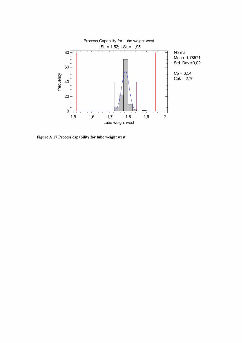
NormalMean=1,78571Std. Dev.=0,020

Cp = 3,54Cpk = 2,70

Process Capability for Lube weight west LSL = 1,52; USL = 1,95

Lube weight west

frequ

ency

1,5 1,6 1,7 1,8 1,9 20

20

40

60

80

Figure A 17 Process capability for lube weight west

Appendix 7 – Design of Experiments

Design-Expert® Sof twarePop-of f pressure

Error f rom replicatesA: Vent ODB: TempC: Time

Positiv e Ef f ects Negativ e Ef f ects

Half-Normal Plot

Hal

f-Nor

mal

% P

roba

bilit

y

|Standardized Effect|

0.00 0.04 0.08 0.12 0.16

0102030

50

70

80

90

95

99

B

C

Figure A 18 Half-Normal Plot Table A 4 ANOVA table from the experiment

ANOVA Analysis of variance table [Partial sum of squares - Type III]

Source Sum of Squares df Mean

Square F

Value p-value

Prob > F

Model 0.083 2 0.042 6.47 0.0213 significant B-Temp 0.034 1 0.034 5.35 0.0494 C-Time 0.049 1 0.049 7.59 0.0249 Curvature 0.016 1 0.016 2.53 0.1504 not significant Residual 0.051 8 6.44E-03 Lack of Fit

2.11E-03 2 1.06E-03 0.13 0.8821 not significant

Pure Error 0.049 6 8.23E-03 Cor Total 0.15 11

Design-Expert® Sof tware

Pop-of f pressure4.025

3.55

X1 = B: TempX2 = C: Time

Actual FactorA: Vent OD = Small

80.00 85.00

90.00 95.00

100.00

3.00

4.00

5.00

6.00

7.00

3.7

3.775

3.85

3.925

4

Pop

-off

pres

sure

B: Temp C: Time

Figure A 19 3D surface graph

Design-Expert® Sof tware

Pop-of f pressureDesign Points4.025

3.55

X1 = B: TempX2 = C: Time

Actual FactorA: Vent OD = Small

80.00 85.00 90.00 95.00 100.00

3.00

4.00

5.00

6.00

7.00Pop-off pressure

B: Temp

C: T

ime

3.75729

3.80521

3.85313

3.90104

3.94896

22

22

22

Figure A 20 Contour graph

Appendix 8 – New flow chart for PTI

Figure A 21 Flow chart for PTI with the task of pulling the cap added

Axles are received

from DGAScanned

Placed in raw material to be

painted

Axles are washed at 150-170º F

Axles are blow-dried at 35 psi

MaskedAxles go

through flash tunnel

Axles go into oven at 200º F

Unloaded

Tagged depending on

defect

Are the axles ok?

Yes

Axles unloaded

Axles are painted at

20 psi

De-masked Stored Loads pulled

Pulled to dock

Taken to sorting area if

needed

Loaded to sequencer

Sent back to AAM

Are the axles ok?

Yes

No

NoPTI defect?

Repaired

No

Yes

Cap pulled to equalize pressure

Appendix 9 – Binomial Probability

Page 1

GMT900 Leaking Vent Tube ProjectStatistical Engineering Summary Report

®

B = Cap REMOVED after paint oven (depressurized).C = Cap NOT REMOVED after paint oven (pressurized).

Required Confidence = 0.95, PA = 0.05Number of tolerable failures = 0, c = 0

Old process failure rate (pph) = 5, p = 0.05

Sample Size, n = 58

Results: 58 parts were tested with 0 failures.

Binomial ProbabilityGMT900 Oil Vent Tube Leak Project

Conclusion: 58 parts were tested and there were no failures. Therefore, the new process is better than the

old process with 95% confidence.

Figure A 22 Binomial Probability

Appendix 10 – Rear Axle Oil Seepage at Vent Cap

11/16/05 Subject: Rear Axle Oil Seepage at Vent Cap 1. Problem was first identified during the first GMT 900 pilot runs at the Janesville Assembly Plant. There was oil seeping from the rear axle between the cap and vent connector opening. Suspect axles were cleaned and monitored to clarify that it was not a leak issue. 2. GM Engineering and SQE representatives visited AAM’s paint processing facility to review axles for this issue. There were a couple axles noted to have some wetness around the vent connector. These were cleaned and confirmed to not seep again. 3. AAM Detroit Gear and Axle has incorporated actions to reduce the number of occurrences for this issue. The following are actions that have been initiated:

a. The GP-12 process has been modified to include the review of all axles for this issue. All axles found with this issue are cleaned, monitored and released based on results after clean-up.

b. The GP-12 process was also modified to include the task of removing the yellow caps from the vent connector for approximately 5 seconds to allow for any pressure buildup to expel from the axle.

c. The standard operating procedure (work instructions) for the NVH EOL tester in Plant 2 has been updated to include the removal of the vent connector cap during the actual test of the axles. This is being done to help in reducing pressure buildup that might happen during the gear rotation at high RPM’s for approximately 1 minute.

d. After completion of the initial GP-12 process for GMT 900’s the task of removing and replacing the cap on the vent connector will be added to the regular final inspection work instructions at the paint processor.

Any questions on the above information can be addressed with the undersigned. S. Wasik DG&A Quality Manager