Leadership in Groups: A Monetary Policy · PDF fileLeadership in Groups: A Monetary Policy ......

Leadership in Groups: A Monetary PolicyExperiment∗

Alan S. Blindera and John Morganb

aPrinceton UniversitybUniversity of California, Berkeley

This paper studies monetary policy decision making bycommittee, using an experimental methodology. In an earlierpaper (Blinder and Morgan 2005), we found that groups notonly outperformed individuals, but they also took no longerto reach decisions. We successfully replicate those results here.Next, we find little difference between the performances of four-person and eight-person groups; the larger groups outperformthe smaller groups by a very small (and often insignificant)margin. Third, and most surprisingly, we find no evidence ofsuperior performance by groups that have designated leaders.Possible reasons for that strongly counterintuitive finding arediscussed.

JEL Codes: C92, E58.

1. Introduction and Motivation

The transformation of monetary policy decisions in most countriesfrom individual decisions to group decisions is one of the mostnotable developments in the recent evolution of central banking(Blinder 2004, ch. 2). In an earlier paper (Blinder and Morgan 2005),we ran an experiment in which Princeton University students, act-ing as ersatz central bankers, made monetary policy decisions bothas individuals and in groups. Those experiments yielded two mainfindings:

∗We are grateful to Jennifer Brown, Jae Seo, and Patrick Xiu for fine researchassistance and to the National Science Foundation and Princeton’s Center forEconomic Policy Studies for financial support. We also acknowledge extremelyhelpful comments from Petra Geraats, Petra Gerlach-Kristen, Jens Grosser, Hel-mut Wagner, a referee, and seminar participants at Princeton, the InternationalMonetary Fund, and the National Bureau of Economic Research.

117

118 International Journal of Central Banking December 2008

(i) Groups made better decisions than individuals, in a sense tobe made precise below.

(ii) Groups took no longer to reach decisions than individuals did.1

The first finding was not a big surprise, given the previous liter-ature on group versus individual decision making (most of it fromdisciplines other than economics). But we were frankly stunned bythe second finding. Like seemingly everyone, we believed that groupsmoved more slowly than individuals. A subsequent replication withstudents at the London School of Economics (Lombardelli, Proud-man, and Talbot 2005) verified the first finding but did not reporton the second one.

This paper replicates our 2005 findings using the same experi-mental apparatus, but with students at the University of California,Berkeley. That the replication is successful bolsters our confidence inthe Princeton results. But that is not the focus of this paper. Instead,we study two important issues that were deliberately omitted fromour previous experimental design.

The first pertains to group size. In the Princeton experiment,every monetary policy committee (MPC) had five members—precisely (and coincidentally) the size that Sibert (2006) subse-quently judged to be optimal. Lombardelli, Proudman, and Tal-bot (2005), following our lead, also used committees of five. Butreal-world monetary policy committees vary greatly in size, so itseems important to compare the performance of small versus largegroups. Revealed-preference arguments offer little guidance in thismatter, since real-world MPCs range in size from three to twenty-one, with the European Central Bank (ECB) headed even higher. Inthis paper, we study the size issue by comparing the experimentalperformances of groups of four and eight.2

1In both our 2005 paper and the present one, “time” is measured by theamount of data required before the individual or group decides to change theinterest rate—not by the number of ticks of the clock. Our reason was (andremains) simple: this is the element of time lag that is relevant to monetarypolicy decisions; no one cares about how many hours the committee meetingslast.

2The reason for choosing even-numbered groups will be made clear shortly.Our “large” groups (n = 8) are still small compared with, e.g., the ECB or theFederal Reserve. This size was more or less dictated by the need to recruit large

Vol. 4 No. 4 Leadership in Groups 119

The second issue pertains to leadership and is the unique aspectof the research reported here. Both our Princeton experiment andLombardelli, Proudman, and Talbot’s replication treated all mem-bers of the committee equally. But every real-world monetary policycommittee has a designated leader who clearly outranks the others.At the Federal Reserve, that leader is the “chairman”; at the ECB,he is the “president”; and at the Bank of England and many othercentral banks, he or she is the “governor.” Indeed, we are hard-pressed to think of any committee, in any context, that does nothave a well-defined leader. Juries come close, but even they haveforemen. Observed reality, therefore, strongly suggests that groupsneed leaders in order to perform well. But is it true? That is themain question that motivates this research.

Consider leadership on MPCs in particular. While all MPCs havedesignated leaders, the leader’s authority varies greatly. The Fed-eral Open Market Committee (FOMC) under Alan Greenspan (butnot under Ben Bernanke) was at one extreme; it was what Blinder(2004, ch. 2) called an autocratically collegial committee, meaningthat the chairman came close to dictating the committee’s decision.This tradition of strong leadership did not originate with Greenspan.Paul Volcker’s dominance was legendary, and Chappell, McGregor,and Vermilyea (2005, ch. 7) estimated econometrically that ArthurBurns’s views on monetary policy carried about as much weight asthose of all other FOMC members combined. At the other extreme,the Bank of England’s MPC is what Blinder (2004) called an indi-vidualistic committee—one that reaches decisions (more or less) bytrue majority vote. Governor Mervyn King has even allowed himselfto be outvoted, partly in order to make this point. In between thesepoles, we find a wide variety of genuinely collegial committees, likethe ECB Governing Council, that strive for consensus. Some of thesecommittees are led firmly; others are led only gently.

The scholarly literature on group decision making, which comesmostly from psychology and organizational behavior, offers relativelylittle guidance on what to expect. And only a small portion of it isexperimental. As a broad generalization, our quick review of the lit-erature led us to expect to find some positive effects of leadership on

numbers of subjects. With groups of four and eight, we needed 252 subjects inall.


group performance—which is the same prior we had before review-ing the literature. But it also led to some doubts about whetherintellectual ability is a key ingredient in effective leadership (Fiedlerand Gibson 2001). Instead, the literature suggests that gains fromgroup interaction may depend more on how well the leader encour-ages other members of the group to contribute their opinions franklyand openly (Maier 1970, Blades 1973, and Edmondson 1999). In aninteresting public goods experiment, Guth et al. (2004) found thatstronger leadership produced better results, although the leaders inthat experiment were selected randomly. We did not find any rele-vant evidence on whether leadership effects are greater in larger orsmaller groups.

With these two issues—group size and leadership—in mind, wedesigned our experiment with four treatments, running ten or elevensessions with each treatment:

(i) four-person groups with no leader, hereafter denoted {n = 4,no leader}

(ii) four-person groups with a leader {n = 4, leader}(iii) eight-person groups with no leader {n = 8, no leader}(iv) eight-person groups with a leader {n = 8, leader}

We summarize our results briefly here because they will be under-stood far better after the experimental details are explained. First,we successfully replicate our Princeton results, at least qualitatively:groups perform better than individuals, and they do not requiremore “time” to do so. Second, we find little difference betweenthe performance of four-person and eight-person groups; the largergroups outperform the smaller groups by a very small (and ofteninsignificant) margin. Third, and most important, we find no evi-dence of superior performance by groups that have designated lead-ers. Groups without such leaders do as well as or better than groupswith well-defined leaders. This is a surprising finding, and we willspeculate on some possible reasons later.

The rest of the paper is organized as follows. Section 2 describesthe experimental setup, which in most respects is exactly the sameas in Blinder and Morgan (2005). Section 3 briefly presents resultscomparing group and individual performance that mostly replicatethose of our Princeton experiment. Sections 4 and 5 focus on the


data generated by decision making in groups, presenting new resultson the effects of group size and leadership, respectively. Then section6 summarizes the conclusions.

2. The Experimental Setup3

Our experimental subjects were Berkeley undergraduates who hadtaken at least one course in macroeconomics. We brought them intothe Berkeley Experimental Social Sciences Lab (Xlab) in groups ofeither four or eight, telling them only that they would be playing amonetary policy game. Except by coincidence, the students did notknow one another beforehand. Each computer was programmed withthe following simple two-equation macroeconomic model—exactlythe same one used in the Princeton experiment—with parameterschosen to resemble the U.S. economy:

πt = 0.4πt−1 + 0.3πt−2 + 0.2πt−3 + 0.1πt−4 − 0.5(Ut−1 − 5) + wt

(1)

Ut − 5 = 0.6(Ut−1 − 5) + 0.3(it−1 − πt−1 − 5) − Gt + et. (2)

Equation (1) is a standard accelerationist Phillips curve. Infla-tion, π, depends on the deviation of the lagged unemployment ratefrom its presumed natural rate of 5 percent, and on its own fourlagged values, with weights summing to one. The coefficient on theunemployment rate is chosen roughly to match empirically estimatedPhillips curves for the United States.

Equation (2) can be thought of as an IS curve with the unem-ployment rate, U , replacing real output (via Okun’s Law). Unem-ployment tends to rise above (or fall below) its natural rate whenthe real interest rate, i − π, is above (or below) its “neutral” value,which is also set at 5 percent. (Here i is the nominal interest rate.)But there is a lag in the relationship, so unemployment responds tothe real interest rate only gradually. Like real-world central bankers,our experimental subjects control only the nominal interest rate,not the real interest rate.

3This section overlaps substantially with section 1.1 of Blinder and Morgan(2005) but omits some of the detail presented there.


The Gt term in (2) is the shock to which our student monetarypolicymakers are supposed to react. It starts at zero and randomlychanges permanently to either +0.3 or −0.3 sometime during thefirst ten periods of play. Readers can think of G as representinggovernment spending or any other shock to aggregate demand. Asis clear from (2), a change in G changes U by precisely the sameamount, but in the opposite direction, on impact. Then there arelagged responses, and the model economy eventually converges backto its natural rate of unemployment. Because of the vertical long-runPhillips curve, any constant inflation rate paired with U = 5% canbe an equilibrium.

We begin each round of play with inflation at 2 percent—whichis also the central bank’s target rate (see below). Thus, prior to theshock (i.e., when G = 0), the model’s steady-state equilibrium isU = 5, i = 7, π = 2. As is apparent from the coefficients in equation(2), the shock changes the neutral real interest rate from 5 percentto either 6 percent or 4 percent permanently. Our subjects—whodo not know this—are supposed to detect and react to this change,presumably with a lag, by raising or lowering the nominal interestrate accordingly.

Finally, the two stochastic shocks, et and wt, are drawn inde-pendently from uniform distributions on the interval [−.25, +.25].4

Their standard deviations are roughly half the size of the G shock.This sizing decision, we found, makes the fiscal shock relatively easyto detect—but not too easy.

Lest our subjects had forgotten their basic macroeconomics, theinstructions remind them that raising the interest rate lowers infla-tion and raises unemployment, while lowering it does the reverse,albeit with a lag.5 In the model, monetary policy affects unemploy-ment with a one-period lag and inflation with a two-period lag; butstudents are not told that. Nor are they told anything else aboutthe model’s specification. They are told that the demand shock willoccur at a random time that is equally likely to be any of periods 1through 10. But they are told neither the magnitude of this shock,nor its direction, nor whether it is permanent or temporary.

4The distributions are uniform, rather than normal, for programming con-venience.

5The instructions are provided in the appendix.


Doubtless, this little model economy is far simpler than theactual economies that real-world central bankers try to manage.However, to the student subjects, who do not know anything aboutthe model, we believe this setup poses perplexities that are compa-rable to those facing real-world central bankers, who are trying tostabilize a much more complex system (e.g., one that includes expec-tational effects) but who also know much more, have far more expe-rience, and have abundant staff support. For example, our experi-mental subjects do not know the transmission mechanism, the lagstructure, whether the price equation is forward looking or backwardlooking, and so on. Nor do they have the benefit of staff forecasts oranalyses.

Despite the model’s seeming simplicity, stabilizing it can betricky in practice. Because of the unit root apparent in equation (1),the model diverges from equilibrium when perturbed by a shock—unless it is stabilized by monetary policy. But lags and modest early-period effects combine to make the divergence from equilibriumpretty gradual and hence less than obvious at first. Once unem-ployment and inflation start to “run away from you,” it can bedifficult to get them back on track. Furthermore, it is not easy todistinguish between the permanent G shock and the transitory eand w shocks that add “noise” to the system. Indeed, the subjectsdo not even know that the G shock is permanent while the othersare i.i.d.

Each play of the game proceeds as follows. We start the systemin steady-state equilibrium at the values mentioned above. The com-puter then selects values for the two random shocks and displays thefirst-period values of U and π, which are typically quite close to thetarget values (U = 5%, π = 2%), on the screen for the subjects tosee. In each subsequent period, new random values of et and wt aredrawn, thereby creating statistical noise, and the lagged variablesthat appear in equations (1) and (2) are updated. At some randomtime, unknown to subjects, the G shock occurs. The computer calcu-lates Ut and πt each period and displays them on the screen, whereall past values are also shown. Subjects are then asked to choose aninterest rate for the next period, and the game continues for twentysuch periods. Students are told to think of each period as a quarter,so the simulation covers “five years.” Each five-year run of the gameis different because of different random draws.


No time pressure is applied; subjects are permitted to take asmuch clock time as they wish to make each decision. As noted above,the concept of time that interests us is the decision lag : the amountof new data the decision maker insists upon before changing theinterest rate. In the real world, data flow in unevenly over calendartime; in our experiment, subjects see exactly one new observation onunemployment and inflation each period. So when we say later thatone type of decision-making process “takes longer” than another, wemean that more data (not more minutes) are required.

To rate the quality of their performances, and to reward subjectsaccordingly, we tell students that their score for each quarter is

st = 100 − 10|Ut − 5| − 10|πt − 2|, (3)

and the score for the entire game (henceforth, S) is the (unweighted)average of st over the twenty quarters. We use an absolute-valuefunction instead of the quadratic loss function that is ubiquitous inresearch on monetary policy (and elsewhere) because quadratics aretoo hard for subjects—even Princeton and Berkeley students—tocalculate in their heads. Notice also that the coefficients in equation(3) scale the scores into percentages, which gives them a natural,intuitive interpretation. Thus, e.g., missing the unemployment tar-get by 0.8 (in either direction) and the inflation target by 1.0 resultsin a score of 100 − 8 − 10 = 82 (percent) for that period.6 At theend of the session, scores are converted into money at the rate of 25cper percentage point. Subjects typically scored 80–84 percent of thepossible points, thus earning about $20–$21.

One final detail needs to be mentioned. To deter excessive manip-ulation of the interest rate (which we observed in testing the appa-ratus in dry runs), we charge subjects a fixed cost of 10 points eachtime they change the rate of interest, regardless of the size of thechange.7 Ten points is a small charge; averaged over a twenty-periodgame, it amounts to just 0.5 percent of the total potential score. Butwe found it to be large enough to deter most of the excessive fid-dling with interest rates. Analogously, researchers who try to derive

6The unemployment and inflation data are always rounded to the nearesttenth. So students see, e.g., 5.8 percent, not, say, 5.83 percent.

7To keep things simple, only integer interest rates are allowed.


the Federal Reserve’s reaction function from the minimization ofa quadratic loss function find that they must add something likek(it − it−1)2 to the loss function in order to fit the data. Withoutthat term, interest rates turn out to be far more volatile than theyare in practice.8

The sessions are played as follows. Either four or eight studentsenter the lab and are read detailed instructions, which they are alsogiven in writing. (See the appendix.) In the case of sessions with adesignated leader, the instructions tell them, among other things,that the person earning the highest score while playing alone in part1 of the experiment will be designated the “leader” (the term weuse) of the group for part 2—where he or she will be rewarded witha doubled score.

Subjects are then allowed to practice with the computer appara-tus for five minutes, during which time they can ask any questionsthey wish. At the end of the practice period, each machine is reini-tialized, and each student is instructed to play twelve rounds of thegame (each lasting twenty “quarters”) alone—without communicat-ing in any way with the other subjects. Once all the subjects havecompleted twelve rounds of individual play, the experimenter calls ahalt to part 1 of the experiment.

In part 2, the same students gather around a single large screento play the same game twelve times as a group. It is here that the ses-sions with and without leaders differ. In leaderless sessions, the rulesare exactly the same as in individual play, except that students arenow permitted to communicate freely with one another—as much asand in any way they please. Everyone in the group is treated alike,and each subject receives the group’s common score.

In sessions with a designated leader, the experimenter begins byrevealing who earned the highest score in part 1, and that studentbecomes the leader for part 2.9 Thus, the criterion for electing lead-ers is purely intellective: the skill of an individual at ersatz monetarypolicymaking. Since the group will perform the identical task, thisselection principle would seem a natural one.

8See, e.g., Rudebusch (2001).9On average, that student scored 10.8 points higher than the others in the

group during part 1 of the experiment, a sizable difference. But students werenot told the leader’s score.


Table 1. The Flow of the Experiment

InstructionsPractice Rounds (no scores recorded)Part 1: Twelve rounds played as individualsPart 2: Twelve rounds played as a group (with or without a leader)Part 3: Twelve rounds played as individualsStudents are paid by check and leave

The meaning of leadership in the experiment is threefold: First,the leader is responsible for communicating (verbally) the group’sdecision to the experimenter—which makes the leader pivotal to thediscussion. Second, the leader faces stronger incentives: his or herscore in part 2 is double that of the other subjects. Third, the leadergets to break any tie vote—which is why we use even-numberedgroups.10 While we recognize that the experimental setup still allowslimited scope for leadership, we judged that this was about all wecould do in a laboratory setting with 11/2 hours of experimentaltime. We return to this issue later.

After twelve rounds of group play, the subjects return to theirindividual computers for part 3, in which they play the game anothertwelve times alone, with no communication with the others. Forfuture reference, table 1 summarizes the flow of each session.

A typical session (of 36 rounds of the game) lasted about 90minutes, and we ran 42 sessions in all, amounting to 252 total sub-jects. (No subject was permitted to play more than once.) Eachof the 21 four-person sessions should have generated 24 individualrounds of play per subject, or 21 × 4 × 24 = 2, 016 in all, plus 12group rounds per session, or 252 in all. Each of the 21 eight-personsessions should have generated twice as many individual observa-tions (hence 4,032 in total), plus another 252 group observations.Thus we have a plethora of data on individual performance but arelative paucity of data on group performance. Since a small num-ber of observations were lost due to computer glitches, table 2 dis-plays the exact number of observations we actually generated for

10In principle, the tie-breaking privilege should be worth more in groups offour than in groups of eight. In practice, however, ties were rare.


Table 2. Number of Observations for Each Treatment

Number of Sessions Individuals Groups

n = 4, no leader 10 960 120n = 4, leader 11 1,032 132n = 8, no leader 10 1,885 120n = 8, leader 11 2,112 132

All Treatments 42 5,989 504

each treatment. Most of this paper concentrates on our new find-ings on the behavior of ersatz monetary policy committees—the 504experimental observations listed in the far right column of table 2.

3. Groups versus Individuals: A Replication

We turn first, and very briefly, to the 5,989 observations on individ-ual performance and, especially, to the comparisons between groupsand individuals that were the focus of Blinder and Morgan (2005).The results here are easy to summarize: for the most part, our newresults with the Berkeley sample replicate what we found earlierwith the Princeton sample.11

To begin with, we found in our Princeton experiment that groups(which were all of size five) turned in better average performancesthan did individuals. Specifically, the average group score was 88.3,while the average individual score was 85.3. The difference of 3points, or 3.5 percent, was highly significant. If we merge all fourof our group treatments in the Berkeley experiment, the averagegroup score is 86.6 versus an average individual score of 81.1. Again,groups do better, but here their advantage is 5.5 points, or 6.8percent—almost twice as large as in the Princeton experiment. Thisperformance gap is also highly significant (t = 11.2).

The following regression confirms that this quantitative (but notqualitative) difference between the two experimental results is signif-icant. Clustering by session to produce robust standard errors yields

11However, the Princeton and Berkeley samples have different statistical prop-erties, including both first and second moments, which is why we abandoned ouroriginal idea of simply merging the two samples.


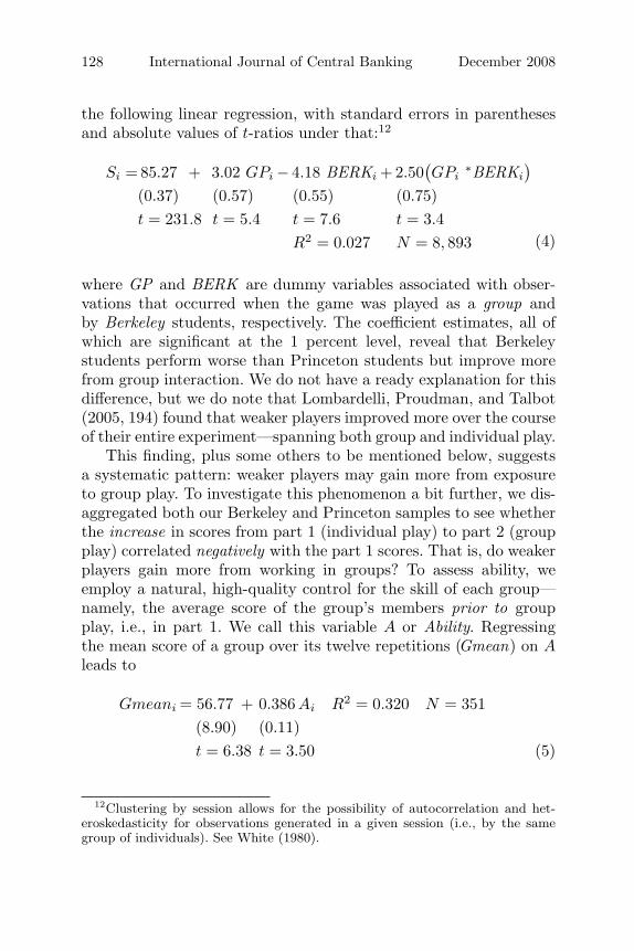
the following linear regression, with standard errors in parenthesesand absolute values of t-ratios under that:12

Si = 85.27 + 3.02 GPi − 4.18 BERKi + 2.50(GPi

∗BERKi

)(0.37) (0.57) (0.55) (0.75)t = 231.8 t = 5.4 t = 7.6 t = 3.4

R2 = 0.027 N = 8, 893 (4)

where GP and BERK are dummy variables associated with obser-vations that occurred when the game was played as a group andby Berkeley students, respectively. The coefficient estimates, all ofwhich are significant at the 1 percent level, reveal that Berkeleystudents perform worse than Princeton students but improve morefrom group interaction. We do not have a ready explanation for thisdifference, but we do note that Lombardelli, Proudman, and Talbot(2005, 194) found that weaker players improved more over the courseof their entire experiment—spanning both group and individual play.

This finding, plus some others to be mentioned below, suggestsa systematic pattern: weaker players may gain more from exposureto group play. To investigate this phenomenon a bit further, we dis-aggregated both our Berkeley and Princeton samples to see whetherthe increase in scores from part 1 (individual play) to part 2 (groupplay) correlated negatively with the part 1 scores. That is, do weakerplayers gain more from working in groups? To assess ability, weemploy a natural, high-quality control for the skill of each group—namely, the average score of the group’s members prior to groupplay, i.e., in part 1. We call this variable A or Ability. Regressingthe mean score of a group over its twelve repetitions (Gmean) on Aleads to

Gmeani = 56.77 + 0.386 Ai R2 = 0.320 N = 351(8.90) (0.11)t = 6.38 t = 3.50 (5)

12Clustering by session allows for the possibility of autocorrelation and het-eroskedasticity for observations generated in a given session (i.e., by the samegroup of individuals). See White (1980).


Notice that the coefficient on the average individual score is con-siderably below unity, implying that Gmean − A, the improvementin group play, is decreasing in A. Thus, consistent with the find-ings of Lombardelli, Proudman, and Talbot (2005), we find thatweaker players improve more than do stronger players from groupinteraction.

The next question pertains to the decision-making lag. How muchtime elapses, on average, between the shock and the monetary pol-icy reaction to it? And do groups display systematically longer lagsthan individuals? Remember, the most surprising result from ouroriginal Princeton experiment was that groups were not slower; infact, they were slightly faster, though not significantly so. Approxi-mately the same is true in our Berkeley experiment. The mean lagsbefore the first interest rate change are essentially identical (roughly3.3 “quarters”) in both group and individual play.

To investigate this question, we create the dependent variableLag, defined as the number of quarters that elapse between the shock(the increase or decrease in G) and the committee’s first interest ratechange. Regression (6) estimates the same specification as (4), butwith Lag replacing S as the dependent variable:

Lagi = 2.45 − 0.15 GPi + 0.75 BERKi + 0.12 GPi∗ BERKi

(0.23) (0.21) (0.28) (0.30)t = 10.7 t = 0.7 t = 2.7 t = 0.4

R2 = 0.007 N = 8,893(6)

This regression shows that groups take about the same amountof time as individuals to reach a decision, as we found before. (TheF -test for omitting the two GP variables has a p-value of 0.69) Italso shows that Berkeley students playing as individuals move moreslowly (by approximately 0.75 “quarters”) than Princeton students.

This demonstrated ability to replicate our earlier resultsenhances confidence in the experimental apparatus. So we turn nowto the two new questions, which pertain to group size and lead-ership. Since the two issues are largely orthogonal, we treat themseparately at first. Later (cf. table 4), we will show that interac-tion effects between group size and leadership are negligible andstatistically insignificant.


Figure 1. Distribution of MPC Size in the Sample

Source: Erhart and Vasquez-Paz (2007)

4. Are Larger Groups More Effective Than SmallerGroups?

The title of our 2005 paper asked metaphorically, are two heads bet-ter than one? We now ask—literally—whether eight heads are betterthan four; i.e., do smaller (n = 4) or larger (n = 8) groups performbetter in conducting simulated monetary policy?

As an empirical matter, most real-world MPCs cluster in thefive- to ten-member range, with some smaller and some larger.13

The most recent study of committee size, by Erhart and Vasquez-Paz (2007), finds that both the mean and median sizes of com-mittees are around seven members. Figure 1, which is taken fromthat paper, also illustrates that the distribution of committee size isasymmetric—with a small but long right-hand tail.14 In addition, it

13See Mahadeva and Sterne (2000).14Erhart and Vasquez-Paz (2007) distinguish between de facto and de jure size,

which do not always match up. Figure 1 shows both.


can be seen that committees with odd numbers of members are farmore common than committees with even numbers. So our largercommittees are somewhat typical of real-world MPCs, while oursmaller committees are clearly on the small side. But does groupsize matter at all?

To focus on size effects, we begin by pooling the data from ses-sions with and without designated leaders—a pooling that our sub-sequent results say is legitimate. Initially, we do not control for theskill levels of the members of the group either. Simply regressing theaverage game score (the variable S defined above) for each of the504 group observations on a dummy for the size of the group, andclustering by session to produce robust standard errors, yields thesimple linear regression shown in column 1 of table 3, with standarderrors in parentheses and asterisks indicating significance levels. The“large-group dummy” is defined to be 1 for eight-person groups and0 for four-person groups. Thus, the regression suggests a small pos-itive effect of larger group size—a score 2.3 points higher for thelarger groups—which is significant if you are not too fussy aboutsignificance levels (the p-value is 0.067).

However, larger groups might simply have drawn, on average,more highly skilled individuals than did smaller groups. So it seemsadvisable to control for the abilities of the various members of thegroup. Fortunately, we have a natural, high-quality control for abil-ity: the average score of all the members of the group prior to theirexposure to group play, i.e., in part 1 of the experiment. This is thevariable A introduced above, and we use both it and its square ascontrols for skill in the column 2 regression. Notice the huge jumpin R2—the Ability variable has high explanatory power.15

Column 2 reveals that controlling for differences in the averageability of members of the larger groups reduces the estimated dif-ference in the performance of large versus small groups by over 40percent—to just 1.3 points. However, even after accounting for theability of group members, larger groups perform significantly better(p-value = 0.08) than smaller groups.

15When the same regression is estimated by ordinary least squares, the coeffi-cients are almost identical, but the standard errors are roughly half of those incolumn 2—indicating that clustering matters.


Tab

le3.

Reg

ress

ion

Res

ults

onG

roup

Siz

e

(1)

(2)

(3)

(4)

(5)

(6)

(7)

Dep

enden

tV

aria

ble

→Sco

reSco

reSco

reSco

reLag

Cor

rect

Fre

quen

cy

Lar

ge-G

roup

Dum

my

2.28

0*1.

292*

1.03

31.

031

−0.

021

−0.

011

−0.

269*

(1.2

11)

(0.7

23)

(0.6

55)

(0.6

57)

(0.4

29)

(0.0

38)

(0.1

50)

Abi

lity

9.62

8***

7.02

7***

7.07

7***

−2.

331*

*0.

006

−0.

133

(3.2

76)

(2.4

21)

(2.6

29)

(0.9

12)

(0.1

14)

(0.3

66)

Abi

lity2

−0.

060*

**−

0.04

4**

−0.

044*

*0.

014*

*0.

000

0.00

1(0

.021

)(0

.016

)(0

.017

)(0

.006

)(0

.001

)(0

.002

)Bes

t2.

023

1.98

1(1

.857

)(1

.902

)Bes

t2−

0.01

0−

0.01

0(0

.012

)(0

.012

)G

roup

Stan

dard

0.02

0D

evia

tion

(0.1

56)

Con

stan

t85

.479

***

−30

0.52

8**

−29

3.16

0***

−29

3.37

0***

97.3

32**

*0.

437*

*6.

068

(1.0

63)

(124

.108

)(8

5.63

0)(8

6.63

0)(3

3.71

8)(4

.256

)(1

3.61

6)

No.

ofO

bser

vati

ons

504

504

504

504

504

504

504

R2

0.03

0.24

0.26

0.26

0.07

0.01

0.03

Note

s:R

obus

tst

anda

rder

rors

clus

tere

dby

sess

ion

are

inpa

rent

hese

s.*,

**,an

d**

*de

note

sign

ifica

nce

atth

e10

per

cent

,5

per

cent

,an

d1

per

cent

leve

l,re

spec

tive

ly.“

Lar

ge-G

roup

Dum

my”

equa

ls1

ifth

egr

oup

cont

aine

dei

ght

mem

ber

s.“A

bilit

y”is

the

aver

age

scor

eof

all

mem

ber

sof

agr

oup

duri

ngpa

rt1

ofth

eex

per

imen

ts.

“Bes

t”is

the

high

est

aver

age

scor

eat

tain

edby

am

ember

ofa

grou

pdu

ring

part

1.“G

roup

Stan

dard

Dev

iation

”is

the

stan

dard

devi

atio

nof

aver

age

part

1sc

ores

.


The estimated quadratic in Ability, by the way, carries an inter-esting and surprising implication: that the contribution of individualability to group performance peaks at A = 80.7 points, which is onlya few points above the average part 1 score of 77.4 points. After that,too many good cooks seem to spoil the broth.

The negative slope beyond A = 80.7 is, however, an artifact ofthe inflexible quadratic functional form. When we estimate insteada freer functional form (such as a spline) that allows the relationshipbetween S and A to flatten out beyond, say, A = 80, we get essen-tially a zero (rather than a negative) slope for high values of A. Still,it is surprising that groups reap no further rewards from the abilitiesof their members once A exceeds a fairly modest level (approxi-mately 80). But this is a robust finding that survives experimentswith several functional forms.16

Let us now return to why larger groups perform (slightly) betterthan smaller groups. One possibility is that a group’s decisions aredominated by its most skilled player.17 Larger groups will, on aver-age, have better “best players” than smaller groups simply becausethe first-order statistic for skill will, on average, be higher whenn = 8 than when n = 4. To see whether that factor might be empir-ically important in these data, we added both the average score ofthe group’s best player (Best) and its square in the regression to getthe regression reported in column 3. We see that the effect of largergroup size is reduced by about 20 percent, and it is now no longersignificant at even the 10 percent level (p = 0.12).

The explanatory power of the Best variables is modest, however.Neither Best nor Best2 is statistically significant on its own, and theestimated coefficients are small compared with those of the A vari-ables. Moreover, adding Best and Best2 raises R2 by only 0.026.18

However, an F -test of the joint hypothesis that the coefficients on

16The surprising thing is not that there are diminishing returns to group size,which can be rationalized in many ways, but that marginal returns seem to getto zero so quickly.

17Several colleagues assured us that this would be the case in our first experi-ment. But we tested and rejected the hypothesis in Blinder and Morgan (2005).

18Surprisingly, the individual score of the second-best player turns out to havemore explanatory power for the group’s performance. We have no ready expla-nation for this finding and treat it as a fluke. Regardless, the results on groupsize are not qualitatively affected under this alternative specification.


both variables are 0 strongly rejects that hypothesis (F = 30.9,p = 0.00).19 Thus, the evidence suggests that the fuller specification(column 3) is preferred, but that the influence of the best player ismodest—a point to which we shall return in considering the effectsof leadership.

Next, we ask whether heterogeneity of the members of the group,as measured by skill differences across players, improves group per-formance. We measure heterogeneity by introducing a new variablein column 4: the standard deviation of the average part 1 scoresobtained by the (four or eight) members of the group.20 Comparingcolumns 3 and 4 shows that adding this variable has essentially noeffect on the regression. Thus heterogeneity does not seem to matter.

4.1 How Do Larger Groups Outperform Smaller Groups?

Having shown that larger groups (barely) outperform smallergroups, the next question is, how do they do it? To determinewhether a shorter or longer decision-making lag is the source ofthe advantage for large groups, we regress the variable Lag definedabove on the dummy for groups of size eight and the ability con-trols mentioned above, clustering by session as usual. The result isthe regression in column 5 of table 3, which indicates no differencebetween the two group sizes in terms of speed of decision making.(The p-value of the coefficient of the dummy is 0.58.) Differences inability are again significant, with groups composed of more skilledplayers tending to decide more quickly—but only until A reaches81.2. Moreover, note the low R2 in this regression, which indicatesthat neither group size nor ability explains much of the variation inlag times.

Next, we turn to accuracy rather than speed. For the regressionin column 6, we define a new left-hand variable, Correct, which is

19This looks like the classic symptoms of extreme multicollinearity, but in factthe correlation between A (the group average) and Best is only 0.67. ReplacingA—which, of course, includes Best—with the median does not reduce the multi-collinearity at all (the correlation between the median and Best is also 0.67), andit generally produces worse-fitting regressions. For these reasons, we stick withthe mean, rather than the median, in what follows.

20This is an admittedly narrow concept of heterogeneity. But, other than thesex composition of the group (which did not matter), it is the only measure ofheterogeneity we have.


equal to 1 if the group’s initial interest rate move is in the correctdirection—i.e., if a rise in G is followed by a monetary tightening,or a decline in G is followed by a monetary easing—and equal to 0otherwise. Do larger groups derive their advantage by being moreaccurate, in this sense?21 Apparently not. The group-size dummyagain shows no difference between groups of size four and size eight.It is interesting to note that, now, the average ability of the membersof the group is also of no use in predicting the group’s success—asurprising finding.

Having failed so far, we turn to one last performance metric:the frequency of interest rate changes. Remember that each changein the rate of interest costs the group a 10-point charge. So it ispossible that larger groups do better because they “fiddle around”less with interest rates. To find out, we define a new left-hand vari-able, Frequency, which measures the number of rate changes a groupmakes over the course of a twenty-quarter game. Since interest ratechanges are costly, it pays for groups to economize on them. Thesimple regression in column 7 reveals a modest effect of group inter-action in producing more “patient” decision making. And, strikingly,the Ability variable seems to have little to do with the frequency ofrate changes.

Here at last we find a partial answer to the question of why largergroups perform slightly better: they average 0.27 fewer interest ratechanges per game (with a p-value of 0.08). Since only about 2.25changes are made on average, this is a meaningful difference.

To summarize this investigation, larger groups take about asmuch time (measured in terms of data) and are about as accurate intheir decisions as smaller groups. However, they make slightly fewerinterest rate changes overall and, in this (limited) sense, are slightlymore “stodgy” decision makers than individuals. This slightly morepatient behavior, in turn, produces a systematic, though quite mod-est, performance advantage over small groups.

21Of course, since Correct is binary, a linear probability specification may notbe appropriate. As an alternative, we could have performed a probit regressionat the cost of not being able to cluster standard errors. The results from probitregressions are qualitatively and quantitatively similar to the linear probabilityspecifications reported here.


Why might larger groups do slightly better? In this environmentof pervasive uncertainty, each member of a group is likely to carryin a somewhat different notion of how the model works from hisor her own experience with individual play—and thus, in particu-lar, a different notion of how often to change interest rates. Groupplay allows members to pool the wisdom gained from their individ-ual experiences. If pooling offers gains, but the gains are subject todiminishing returns, we might find groups of eight outperforminggroups of four.

But then why are the gains from larger group size so small?One possibility might be that the optimal committee size is, say,n = 6. In that case, committees of four (too small) and eight (toolarge) might be almost equally suboptimal.22 Alternatively, it couldbe that n = 4 and n = 8 are simply too close together, and thatexperimenting with, say, n = 12 or more might have producedlarger differences. Finally, it is worth noting that our committees areall symmetric—everyone does exactly the same thing. By contrast,many real-world MPCs allow (or require) their members to specializein certain tasks. Diminishing returns presumably sets in more slowlyin such specialized committees than in symmetric committees.

5. Does Leadership Enhance Group Performance?

As noted in the introduction, virtually all decision-making groups inthe real world, and certainly all MPCs, have well-defined leaders—e.g., the chairman of a committee. To an economist, or to a Dar-winian evolutionist for that matter, this observation creates a strongpresumption that leadership must be productive—for why else wouldit be so ubiquitous? But, as we show now, our experimental findingssay otherwise: surprisingly, groups with designated leaders do notoutperform groups without leaders.

We start table 4, as we did table 3, with a simple regressioncomparing the scores of groups with and without leaders—ignoring,for the moment, both average ability and group size. The leaderdummy, defined to be 1 if the group has a designated leader and 0otherwise, actually gets a negative (though insignificant) coefficient

22This possibility was suggested to us by Petra Geraats.

Vol. 4 No. 4 Leadership in Groups 137Tab

le4.

Reg

ress

ion

Res

ults

onLea

der

ship

(1)

(2)

(3)

(4)

(5)

(6)

(7)

(8)

Dep

enden

tV

aria

ble

→Sco

reSco

reSco

reSco

reLag

Cor

rect

Fre

quen

cySco

re

Lea

der

Dum

my

−0.

832

−0.

160

−0.

287

−0.

025

0.15

4−

0.71

8(1

.225

)(0

.742

)(0

.415

)(0

.033

)(0

.152

)(1

.098

)A

bilit

y10

.300

***

12.2

57*

17.8

20**

*−

2.37

7***

0.00

9−

0.25

99.

430*

**(3

.515

)(6

.098

)(4

.138

)(0

.822

)(0

.102

)(0

.347

)(3

.182

)A

bilit

y2−

0.06

4***

−0.

078*

−0.

114*

**0.

015*

*0.

000

0.00

2−

0.05

8***

(0.0

23)

(0.0

41)

(0.0

28)

(0.0

06)

(0.0

01)

(0.0

02)

(0.0

21)

Bes

t−

0.38

4(2

.697

)Bes

t20.

005

(0.0

17)

Fem

ale

−1.

164

(1.1

00)

Lar

ge-G

roup

0.76

9D

umm

y(0

.837

)Lar

geG

roup

×1.

045

Lea

der

(1.4

39)

Con

stan

t87

.054

***

−32

5.40

5**

−39

3.58

7*−

609.

677*

**99

.346

***

0.35

210

.582

−29

2.00

1**

(0.6

13)

(133

.642

)(2

02.2

19)

(153

.455

)(3

0.25

1)(3

.825

)(1

3.02

9)(1

20.9

57)

No.

ofO

bser

vati

ons

504

504

264

252

504

504

504

504

R2

0.01

0.23

0.32

0.32

0.07

0.01

0.02

0.03

Note

s:R

obus

tst

anda

rder

rors

clus

tere

dby

sess

ion

are

inpa

rent

hese

s.*,

**,an

d**

*de

note

sign

ifica

nce

atth

e10

per

cent

,5

per

cent

,an

d1

per

cent

leve

l,re

spec

tive

ly.“L

eade

rD

umm

y”eq

uals

1if

the

grou

pha

da

desi

gnat

edle

ader

.“A

bilit

y”is

the

aver

age

scor

eof

all

mem

ber

sof

agr

oup

duri

ngpa

rt1

ofth

eex

per

imen

t.“B

est”

isth

ehi

ghes

tav

erag

esc

ore

atta

ined

bya

mem

ber

ofa

grou

pdu

ring

part

1.“F

emal

e”eq

uals

1if

the

lead

erw

asa

fem

ale.

“Lar

ge-G

roup

Dum

my”

equa

ls1

ifth

egr

oup

cont

aine

dei

ght

mem

ber

s.


in column 1. Once we control for ability in column 2, this smallcoefficient drops to virtually zero, and the effect of ability on groupperformance resembles that in table 3—a quadratic in A that peaksat 80.4. Thus the counterintuitive finding is that leadership does notaffect group performance. We proceed now to try to overturn thissurprising non-result.

One obvious explanation might be that our designated leadersachieve their high scores during part 1 purely by chance, and thusare really no more able than the others. This possibility is easilydismissed, however, by looking at scores in part 3 of the game—when subjects play again as individuals. Across all individuals whoparticipated in the sessions with designated leaders, the correlationbetween their part 1 scores and their part 3 scores is 0.45, indicatingsubstantial and durable individual effects. Thus it is not just luck;the leaders really are better.

One interesting question to ask, once again, is whether thegroup’s score is driven more by the skill of the average memberor by the skill of the leader. To address this question, we restrictour attention in column 3 to sessions with designated leaders (thusreducing the sample size to 264) and add the previously defined vari-ables Best and Best2 to the regression. Remember that Best is theaverage score of the highest-scoring individual in part 1—and thusthe score of the designated the leader in part 2.

Interestingly, the average skill of the group’s members (“Abil-ity”) is a much better predictor of performance than the skill of theleader (“Best”). To see this formally, we ran F -tests to determinethe effect of omitting the two Ability variables versus omitting thetwo Best variables from the regression. For the Ability variables,the F -statistic is 8.7 (p = 0.00) whereas for the Best variables, theF -statistic is only 3.2 (p = 0.06). The comparative weakness of theBest variables illuminates the puzzling absence of leadership effectson performance: while the leader is the best player, he or she seemsincapable of improving the performance of the group.23

We next ask whether leadership effects on group performance dif-fer by the gender of the leader by adding a dummy variable Female

23The inverted quadratic in Best seen in column 3 looks peculiar, but it isupward sloping in the relevant range. Given the imprecision of the estimates ofthese coefficients, one shouldn’t make much of this result.


to the regression in column 4. Again, we restrict our attention tosessions with designated leaders.24 While the estimated coefficientfor female leaders is negative, it does not come close to statisticalsignificance. Thus, women do neither better nor worse as leaders.25

So leaders seem to have no discernible effect on their group’sscore. But do they influence the group’s strategy? To examine thisquestion, we look next at the dependent variable Lag defined ear-lier. Column 5 shows that leadership does not influence the speed ofreaction significantly. While the coefficient of the leader dummy isnegative, it is insignificant.

What about leadership effects on the likelihood of moving in thecorrect direction on the first interest rate change? The column 6regression also shows essentially no effect.

Finally, we turn to the frequency of rate changes. Do groups withdesignated leaders change interest rates more (or less) frequently?The answer is (weakly) more frequently, as the regression in column7 shows. But, again, the effect does not come close to statisticalsignificance.

To this point, we have looked for leadership effects on the (tacit)assumption that they are the same in large (n = 8) and small (n =4) groups. Similarly, in the previous section we examined the effectsof group size while maintaining the hypothesis that size effects arethe same with and without leaders. To test for possible interactioneffects, the last regression in table 4 includes dummies for both groupsize and leadership, allowing an interaction between the two.

Column 8 reveals that the interaction effect is totally insignifi-cant (p-value = 0.47). Still, if the positive coefficient is taken at facevalue, the regression suggests a small negative effect of leadership insmaller groups and a small positive effect in larger groups.

A fair summary so far would be to say that you need a mag-nifying glass—and you must ignore statistical significance—to seeany effects of leadership on group performance. The main message,surprisingly, is that leadership does not seem to matter.

24A leader in one of the eight-person sessions refused to identify his or hergender, which reduced the number of observations to 252.

25They are also neither better nor worse as followers. The sex composition ofthe group does not help explain the group’s performance.


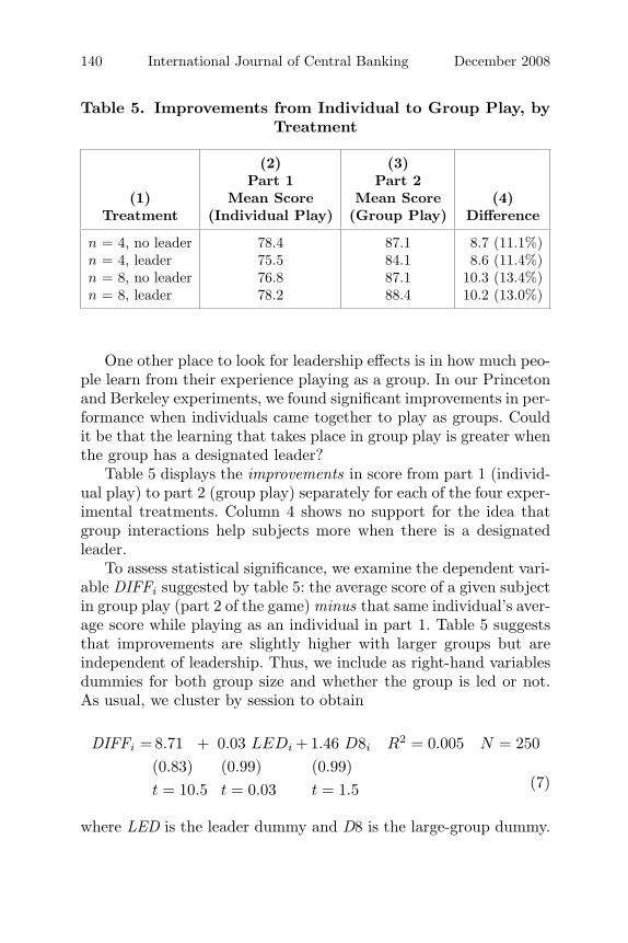
Table 5. Improvements from Individual to Group Play, byTreatment

(2) (3)Part 1 Part 2

(1) Mean Score Mean Score (4)Treatment (Individual Play) (Group Play) Difference

n = 4, no leader 78.4 87.1 8.7 (11.1%)n = 4, leader 75.5 84.1 8.6 (11.4%)n = 8, no leader 76.8 87.1 10.3 (13.4%)n = 8, leader 78.2 88.4 10.2 (13.0%)

One other place to look for leadership effects is in how much peo-ple learn from their experience playing as a group. In our Princetonand Berkeley experiments, we found significant improvements in per-formance when individuals came together to play as groups. Couldit be that the learning that takes place in group play is greater whenthe group has a designated leader?

Table 5 displays the improvements in score from part 1 (individ-ual play) to part 2 (group play) separately for each of the four exper-imental treatments. Column 4 shows no support for the idea thatgroup interactions help subjects more when there is a designatedleader.

To assess statistical significance, we examine the dependent vari-able DIFFi suggested by table 5: the average score of a given subjectin group play (part 2 of the game) minus that same individual’s aver-age score while playing as an individual in part 1. Table 5 suggeststhat improvements are slightly higher with larger groups but areindependent of leadership. Thus, we include as right-hand variablesdummies for both group size and whether the group is led or not.As usual, we cluster by session to obtain

DIFFi = 8.71 + 0.03 LEDi + 1.46 D8i R2 = 0.005 N = 250(0.83) (0.99) (0.99)t = 10.5 t = 0.03 t = 1.5 (7)

where LED is the leader dummy and D8 is the large-group dummy.


Table 6. Improvements from Part 1 to Part 3,by Treatment

(2) (3)Part 1 Part 3

Mean Score Mean Score(1) (Individual (Individual (4)

Treatment Play) Play) Difference

n = 4, no leader 78.4 83.2 4.8 (6.1%)n = 4, leader 75.5 85.2 9.7 (12.8%)n = 8, no leader 76.8 85.1 8.3 (10.8%)n = 8, leader 78.2 84.9 8.7 (8.6%)

This regression shows that leadership has no effect on the improve-ment between individual and group play. On the other hand,participation in larger groups does improve upon individual perfor-mance slightly more than participation in smaller groups; however,the result does not quite rise to the level of statistical significance(p = 0.15).

One final question about leadership and learning can be raised.We found in both experiments that scores typically improve quitea bit when subjects move from individual play to group play (frompart 1 to part 2) but then fall back somewhat when they return toindividual play (from part 2 to part 3). The change in an individual’sperformance from part 1 to part 3 can therefore be used as an indi-cator of what might be called the “durable learning” that emergesfrom experience with group play. Is this learning greater when thegroup has a designated leader than when it does not?

Table 6 suggests that the answer is no. The subjects learn morefrom group play with a designated leader when n = 4, but less whenn = 8. Notice, by the way, that the largest improvement in table 6comes in the {n = 4, leader} groups—the treatment that, by chance,got the weakest players.

The statistical significance of this result can be appraised byregressing the dependent variable POSTDIFFi, defined as the dif-ference between the average score of a given subject in part 3 of thegame less that same individual’s average score in part 1, on dummy


variables for leadership and size. Clustering by session as usual, theresult is

POSTDIFFi = 7.38 + 0.41 LEDi− 0.18 D8i R2 = 0.00 N = 250(1.13) (1.21) (1.21)t = 6.5 t = 0.3 t = 0.2 (8)

This regression shows that neither group size nor leadership affectsthe durable performance gains that arise from exposure to groupplay.

In sum, there is no evidence from our experiment of superior (oreven faster) performance by groups with designated leaders versusgroups without. Overall, the most prudent conclusion appears tobe that groups with designated leaders perform no differently thangroups without leaders. This is a surprising finding, to say the least.Should we believe it? Maybe, but maybe not.

5.1 Why No Leadership Effects?

First, in defense of our experimental design, remember that we donot choose the leaders randomly or arbitrarily. Rather, each desig-nated leader earns his or her position by superior performance inthe very task that the group will perform. This principle for selectingleaders, we believe, imbues them with a certain legitimacy—as isnormally the case in real-world groups. A second element of realismderives from the reward structure. Doubling the leader’s reward ingroup play gives him or her a greater stake in the outcome—justas leaders of real-world groups normally have greater stakes in theoutcome than other members do. For example, history will appraisethe performance of the “Bernanke Fed” and the “Roberts Court.”The names of most of the other members will be lost to history.

Second, however, while giving the leader the tie-breaking voteallows him or her to influence the group’s decisions in principle, itmay not do so in practice. For example, we found in Blinder andMorgan (2005) that there was no difference in either the quality orspeed of group decision making when groups made decisions unani-mously rather than by majority rule. And, as noted earlier, tie voteswere rare in this experiment.


Third, and in a similar vein, we are able to test only for dif-ferences between groups with and without an officially designatedleader; we have no independent measurement of how effective lead-ership is. Thus, some of our putative leaders may actually be quitepassive, while strong leadership could emerge spontaneously in someof the groups without a designated leader.

Fourth, it should be noted that the task in our experimentalsetup is what psychologists call intellective (figuring something out)rather than, say, judgmental or moral (deciding what’s right andwrong). So the surprising conclusion that leadership in groups hasno apparent benefits should, at the very least, be limited to suchintellective tasks. As Fiedler and Gibson (2001, 171) pointed out,“Extensive empirical evidence has shown that a leader’s intellectualability or experience does not guarantee good [group] performance.”That said, making monetary policy decisions is, for the most part,an intellective task.

Fifth, however, there is never any disagreement among membersof our ersatz MPCs over what the group’s objectives are (includ-ing the relative weights). Every player tries to maximize exactlythe same function. By contrast, there is potential for disagreementover the central bank’s objectives and/or weights on at least somereal-world MPCs (e.g., the FOMC)—which might allow more scopefor effective leadership. In fact, this raises a broader issue. Our stu-dent subjects are arguably a more homogeneous group than at leastsome MPCs, to which people of diverse backgrounds are deliberatelyappointed.

Sixth, and related, our committees deal only with “normal” mon-etary policy decisions. It is certainly possible that greater scope forleadership might emerge if our experimental subjects were faced withcrises, such as the ones the Federal Reserve and the ECB have beenconfronted with in 2007 and 2008.

Finally, and perhaps most important, our narrow experimentalconcept of leadership—leading the discussion, reporting the group’sdecision, and breaking a tie if necessary—does not correspond to thecommon meaning of “leadership” as expressed, e.g., in the admit-tedly chauvinistic statement “He’s a leader of men.” Our exper-imental leaders do not lead in the sense that a military officerleads a platoon, a politician leads a party, or an executive leadsa business. Brown, Scott, and Lewis (2004) classified leaders as


“transformational” and “transactional,” the latter meaning moti-vating subordinates with rewards. Our experimental leaders wereneither.

We thought about trying to select group leaders by what mightloosely be described as “leadership qualities” but quickly abandonedthe idea as being too subjective and too difficult. We think this deci-sion was the right one. But, in interpreting the experimental results,it is important to remember that our leaders are selected, on aver-age, for their “smarts,” not for their “leadership qualities.” There isno reason to think that the cognitive ability we use to select groupleaders correlates highly with the traits that are associated withleadership in the real world, such as verbal dexterity, aggressive-ness, an extroverted personality, a trustworthy affect, good looks,and height. However, we certainly hope (and believe) that cogni-tive ability is a relevant consideration in the selection of real-worldcentral bank heads.

Similarly, it seems plausible that true—as opposed to putative—leadership in groups may need to emerge slowly over time, as theleader demonstrates good performance and as other members growto respect his or her judgment, acumen, and group-managementskills. A one-time, ninety-minute laboratory experiment leaves noscope for that sort of leadership to emerge.

Thus we certainly do not believe that our experimental resultsprovide the last word on leadership effects. We offer them as some-thing closer to the first word, and invite other researchers to pick upthe challenge.

6. Conclusions

In this paper, we replicate earlier findings from Blinder and Mor-gan (2005) showing that simulated monetary policy committeesmake systematically better decisions than the same individuals mak-ing decisions on their own, without taking any longer to do so.This experimental evidence supports the observed worldwide trendtoward making monetary policy decisions by committees, ratherthan by lone-wolf central bankers. We also find several suggestiveshreds of evidence that the margin of superiority of groups overindividuals is greater when the individuals are of lower ability.


But the more novel findings of this paper pertain to groups thatdiffer in terms of size and leadership. We find some weak evidencethat larger groups (in our case, n = 8) outperform smaller groups(n = 4), mainly because larger groups seem better able to resist thetemptation to “fiddle” with interest rates too much. But these dif-ferences are small, and many are not statistically significant. So, interms of institutional design, it is not clear whether larger or smallerMPCs are to be recommended. (Remember that n = 7 is the meanand modal size of real-world MPCs.)

Our most surprising and important result, at least to us, is thatersatz MPCs do not perform any better when they have a designatedleader than when they do not—even though every real-world MPChas a clear (and sometimes dominant) leader, and even though ourdesignated leaders were chosen on the basis of their skill in makingmonetary policy. We caution that we would not apply this findingbeyond the realm of intellective tasks—e.g., we do not recommendthat army platoons venture out without a commanding officer!

But that said, there are probably many more intellective thancombative tasks in the economic world, certainly including mone-tary policy. For example, promotions in business are often based onsuperior performance on metrics that are basically intellective. Sothis finding, if verified by other work, is potentially of wide appli-cability. In terms of the taxonomy of MPCs emphasized by Blinder(2004), our results suggest that an individualistic committee, wherethe leader is only modestly more important than the other members,may function just as well as a collegial committee, where the role ofthe leader is more pronounced.

Appendix. The Instructions

Note: Portions of the instructions read only during sessions withleaders are enclosed in brackets.

In this experiment, you make decisions on monetary policy fora simulated economy, much like the Federal Reserve does for theUnited States. At first, you will make the decisions on your own;later, we will bring you all together to make decisions as a group.[At that point, one of you will be designated the leader of the group,as I will explain shortly.]


We have programmed into each computer a simple model econ-omy that generates values of unemployment and inflation, periodby period, for twenty periods. Think of each period as a calendarquarter, so the game represents five years. Each quarterly value ofunemployment and inflation depends on the interest rates you chooseand on some random influences that are beyond your control. Everymachine has exactly the same model of the economy, but each ofyou will get different random drawings and so will have differentexperiences.

Your goal is to keep unemployment as close to 5 percent, andinflation as close to 2 percent, as you can—quarter by quarter. Asyou can see from the top line on the screen, we start you off with aninterest rate of 7 percent in period 1. Initially, unemployment andinflation differ slightly from the targets of 5 percent and 2 percentbecause of the random influences I just mentioned. Starting withperiod 2, you must choose the interest rate.

Raising the interest rate will increase unemployment anddecrease inflation. But the effects are delayed—neither unemploy-ment nor inflation responds immediately. Similarly, lowering theinterest rate will decrease unemployment and increase inflation. But,once again, the effects are delayed.

The computer determines your score for each period as follows.Hitting 5 percent unemployment and 2 percent inflation exactlyearns you a perfect score of 100 points. For each tenth-of-a-pointby which you miss each target, you lose a point on your score.Direction doesn’t matter; you lose the same amount for being toohigh as for being too low. Thus, for example, 5.8 percent unem-ployment and 1.5 percent inflation will net you a score of 100minus 8 points for missing the unemployment target by eight-tenths minus 5 points for missing the inflation target by five-tenths,or 87 points. Similarly, 3.5 percent unemployment and 3 percentinflation will net you 100 − 15 − 10, or 75 points. If you look atthe top line of the display, you can see that the initial unemploy-ment rate of 5 percent and inflation rate of 1.9 percent yields ascore of 99.

Finally, there is a cost of 10 points each time you change theinterest rate. The 10 points will be deducted from that period’sscore.

Are there any questions about the scoring system?


As you progress through the experiment, accumulating pointsboth in individual and in group play, the computer will keep trackof your cumulative average score on the 1–100 scale. At the end ofthe session, your cumulative average score will be translated intomoney at the rate of 25 c per point, and you will be paid your win-nings by check. Thus a theoretical perfect score of 100 would netyou $25, an average score of 80 would give you 80 percent of $25,or $20, etc. You are guaranteed a minimum of $15, no matter howbadly you do.

[When you play as individuals, everyone is treated the same. Butwhen we bring you together to play as a group, one of you will serveas the group’s leader. The leader will be the one who scored thehighest in individual play, and he or she will receive twice as manypoints during group play.]

The game works as follows. You can move the interest rate upor down, in increments of 1 percentage point, by moving the slidebar on the left-hand side of the screen, or by clicking on the upor down buttons. Try that now to see how it works. When youhave selected the interest rate you want, click on the button marked“Click to Set Rate.” Do that now to see how it works. The computerhas recorded your choice, drawn the random numbers I mentionedearlier, and calculated that period’s unemployment, inflation, andscore.

There is one final, important aspect to the game. At atime period selected at random, but equally likely to be any ofthe first ten periods, aggregate demand will either increase ordecrease. You will not be told when this happens nor in whichdirection.

If aggregate demand increases, that tends to push unemploymentdown and, with a lag, inflation up. If aggregate demand decreases,that tends to push unemployment up and, with a lag, inflation down.The essence of your job is to figure out when and how to adjust inter-est rates in order to keep unemployment as close to 5 percent, andinflation as close to 2 percent, as possible.

Remember, the change in aggregate demand comes at a ran-domly selected time within the first ten periods, and we will not tellyou whether demand has gone up or down. And each interest ratechange will cost you 10 points in the period you make it.

Are there any questions?


Please sign the consent form located in the folder next to yourcomputer.

This will all be simpler once you’ve practiced on the apparatusa bit. You can do so now, and your scores will just be displayedfor your information; they will not be recorded or counted. Youcan practice for about five minutes to develop some familiarity withhow the game works. During this practice time, feel free to ask anyquestions you wish.

OK, it’s time to start the game for real now.In the first part of the experiment, you will play the monetary

policy game twelve times by yourselves. After you have played thegame twelve times, the computer will prevent you from going on.You may not communicate with any other player, and the pointsyou earn will be your own.

[As I mentioned, the student who earns the highest score in thispart of the experiment will be the leader of the group in the nextpart.]

Please start now by clicking the continue button, and proceed atyour own pace.

Now please gather around the projection screen to play thesame game as a group. [The highest scoring player will be theleader.]

In this part of the experiment, you will play exactly the samegame twelve times. The rules are the same except that decisions arenow made by majority rule. [In case of a tie, the leader will castthe tie-breaking vote. The leader will control the mouse.] You maycommunicate freely with each other, as much as and in any way youwish. While playing as a group, each of you will receive the group’sscore [except the leader, who will earn twice as many points]. At theconclusion of group play, we will show you how your performancecompared with the top scores achieved when we ran this game atPrinceton. Any questions?

Please begin.

OK. Now please return to your individual seats and, once again,play twelve rounds of the game by yourselves. Communication with


other players is not allowed. The computer will again stop you aftertwelve rounds.

Please begin.

OK. The experiment is now over. Thank you for participating.

References

Blades, J. W. 1973. “Influence of Intelligence.” In The Influenceof Intelligence, Task Ability, and Motivation on Group Perfor-mance, ed. J. W. Blades and F. E. Fiedler, 76–78. University ofWashington, Seattle: Organizational Research Technical Report.

Blinder, A. S. 2004. The Quiet Revolution: Central Banking GoesModern. New Haven, CT: Yale University Press.

Blinder, A. S., and J. Morgan. 2005. “Are Two Heads BetterThan One? Monetary Policy by Committee.” Journal of Money,Credit, and Banking 37 (5): 789–812.

Brown, D., K. Scott, and H. Lewis. 2004. “Information Processingand Leadership.” In The Nature of Leadership, ed. R. Sternberget al. New York, NY: Sage Publications.

Chappell, H. W., Jr., R. R. McGregor, and T. Vermilyea. 2005.Committee Decisions on Monetary Policy. Cambridge, MA: MITPress.

Edmondson, A. 1999. “Psychological Safety and Learning Behav-ior in Work Teams.” Administrative Science Quarterly 44 (4):350–83.

Erhart, S., and J. L. Vasquez-Paz. 2007. “Optimal Monetary PolicyCommittee Size: Theory and Cross-Country Evidence.” Paperpresented at Norges Bank conference.

Fiedler, F. E., and F. W. Gibson. 2001. “Determinants of EffectiveUtilization of Leader Abilities.” In Concepts for Air Force Lead-ership, ed. R. I. Lester and A. G. Morton, 171–76. Maxwell AirForce Base, AL: Air University Press.

Guth, W., M. Vittoria Levati, M. Sutter, and E. van der Heijden.2004. “Leadership and Cooperation in Public Goods Experi-ments.” Discussion Paper on Strategic Interaction No. 2004-29,Max Planck Institute of Economics.


Lombardelli, C., J. Proudman, and J. Talbot. 2005. “Committeesversus Individuals: An Experimental Analysis of Monetary Pol-icy Decision Making.” International Journal of Central Banking1 (1): 181–205.

Mahadeva, L., and G. Sterne, ed. 2000. Monetary Policy Frameworksin a Global Context. New York, NY: Routledge Publishers.

Maier, N. R. F. 1970. Problem Solving and Creativity in Individualsand Groups. Belmont, CA: Brooks/Cole.

Rudebusch, G. 2001. “Is the Fed Too Timid? Monetary Policy in anUncertain World.” Review of Economics and Statistics 83 (2):203–17.

Sibert, A. 2006. “Central Banking by Committee.” InternationalFinance 9 (2): 145–68.

White, H. 1980. “A Heteroskedasticity-Consistent CovarianceMatrix Estimator and a Direct Test for Heteroskedasticity.”Econometrica 48 (4): 817–38.

Leadership in Groups: A Monetary Policy · PDF fileLeadership in Groups: A Monetary Policy ......

Documents

Transcript of Leadership in Groups: A Monetary Policy · PDF fileLeadership in Groups: A Monetary Policy ......