lcbs working paperspapers volume one -...
84
volume one working papers papers lcbs ISSN 2470-6272
Transcript of lcbs working paperspapers volume one -...

volumeone
workingpaperspapers
lcbs
ISSN 2470-6272

About the Lemann Center for Brazilian Studies (LCBS)
Columbia’s Center for Brazilian Studies, was established in 2001 to offer a place for scholars and
students to pursue and share research and scholarship on Brazil. In 2015, the Center was renamed the
Lemann Center for Brazilian Studies (LCBS). In carrying out its academic mission, the LCBS stimulates
new research and debate on Brazil. The Center is committed to training future leaders for careers in
research, government, and the private sector related to Brazil. Serving as the key focal point for all
students and faculty at Columbia with interest in Brazil, the LCBS’s largest constituencies include those
affiliated with Columbia’s School of International and Public Affairs and from the numerous academic
units of the Graduate School of Arts and Sciences.
The LCBS’s rich programming includes sponsored seminars and lectures on contemporary and historical
aspects of Brazil, including culture, economics, and politics. The LCBS serves as a regular forum for
lectures and conferences by visiting Brazilian academics, government officials, business leaders,
politicians, and representatives of civil society.
In addition to public programming, the LCBS organizes courses focused on Brazil, including courses on
the economic and political development of Brazil, as well as a variety of other topics. The LCBS’s Ruth
Cardoso Visiting Faculty program brings leading Brazilian scholars to the campus for one or two
semester residencies during which they conduct collaborative research and teach courses at the LCBS
in their area of specialization.
Through its Visiting Scholars and Professional Fellows programs, the LCBS offers Brazilian academic
and policy experts the opportunity to be in residence on the Columbia campus and to interact with
members of the Columbia faculty with expertise on Brazil and Latin America.
The LCBS also helps to promote collaborations between the Columbia community and Brazilian
scholars and institutions, working closely with the Columbia University Global Center Rio de Janeiro.
The Lemann Center for Brazilian studies provides support for Columbia faculty research with a focus on
Brazil, as well as engages in original research. The LCBS, for example, has recently published a report
on “Mobile Learning in Brazil”, which examines policies and initiatives for the integration of information
and communication technologies in public schools throughout Brazil. For additional information about
the Lemann Center for Brazilian studies please visit:
http://ilas.columbia.edu/centers-and-programs/brazil-center/

2 | L e m a n n C e n t e r f o r B r a z i l i a n S t u d i e s W o r k i n g P a p e r s | M a r c h 2 0 1 6
About the Lemann Center for Brazilian Studies (LCBS) Working Papers
This Working Papers Series are coordinated by the Lemann Center for Brazilian Studies (LCBS) at
Columbia University in the City of New York. They disseminate policy reports, academic articles, and
preliminary research results encompassing relevant topics about Brazil from a variety of disciplinary
perspectives. We welcome submissions from Columbia faculty and graduate students, as well as visiting
scholars affiliated with the LCBS. Alumni students and scholars may also submit papers.
The Working Papers represents the research and the views of the authors. It does not necessarily
represent the views of the Lemann Center for Brazilian Studies.
ISSN-2470-6272
Table of Contents
1) Development Banking in Brazil: Challenges and Limits
Luiz Pinto & Marcos Reis………………………………………………………...................................Page 3
2) Fiscal policy in Brazil: from Counter-Cyclical Response to Crisis
Márcio Holland…………………………………………………………………………………………………Page 19
3) Reserve Requirements as a Macroprudential Instrument in Brazil and Colombia: Some Empirical
Evidence
Míriam O. S. Português & Antonio Luis Licha.................................................................Page 58

3 | L e m a n n C e n t e r f o r B r a z i l i a n S t u d i e s W o r k i n g P a p e r s | M a r c h 2 0 1 6
Development Banking in Brazil: Challenges and Limits
Luiz Pinto1 and Marcos Reis2
Abstract: This article examines the origins and evolution of long-term financing in Brazil. The need for government intervention in the form of a development bank is explained. Particularities of the Brazilian experience with its state-owned National Development Bank (BNDES) are described and analyzed. The final section tackles the challenges and limitations of the Brazilian system of long-term financing following the global credit crunch of 2008, when BNDES disbursements boomed because of major but unsustainable changes in its capital structure. The article concludes that the system for development finance in Brazil needs to be reformed in order to increase its efficiency and contribute to macroeconomic stability.
Keywords: development banks; long-term finance; BNDES; Brazil
1. Introduction
Global economic geography would probably be different if emerging market-based private groups and state-owned companies did not have the support of development banks. By fusing public policy with capital mobilization and investment management, development banks were crucial to boost catch-up industrialization and import substitution policies in Asia, Latin America, Africa and the Middle East. However, globalization, macroeconomic stabilization, financial market integration and capital market development forged major changes in the nature of development banks.
This paper aims to discuss the role of the Brazilian National Development Bank (BNDES) in the country’s evolving system for long-term finance. The paper is therefore structured in six sections, of which this introduction is the first. The second presents key concepts and definitions, establishing the baselines for theoretical and historical discussions on long-term finance and development banks. The third explains the origins of the BNDES and its remarkable record fostering industrial ventures and import substitution policies. BNDES support for economic modernization, market reforms and privatization during the 1990s and mid-2000s is analyzed in section four, while unorthodox policies designed to use BNDES as a post-Lehmann counter-cyclical tool are discussed in section five. Finally, section six outlines the concluding remarks.
2. Long-Term Finance and Development Banks
Development finance is the art of gathering funds to pay for multiyear payback capital-intensive undertakings. Mostly, these long-dated funds are deployed in different sorts of large-scale projects, including real estate enterprises, infrastructure, education, research, and the acquisition of capital goods, equipment and software. They are important to create jobs, expand production and increase productivity (G30, 2013).
Private sources such as commercial banks and capital markets supply most of the services for development finance demanded by developed economies. However, private sources are not able to fulfill the overall demand for funding, and especially so in emerging and developing economies, where market failures are often more relevant.
Long-term financing supply is significantly affected by the following market failures:
a) Financial markets incompleteness: because of their history of high inflation, depreciation and interest rate volatility, emerging and developing markets often suffer from so-called “original sin,” that is, a situation in which a domestic currency has a very low demand from non-residents, being unable to be used to borrow
1 Executive Director of BRICS Overseas, he holds a Ph.D. in International Political Economy and is a Visiting Scholar at the School of International and Public Affairs at Columbia University, New York. 2 Associate professor at the National Institute of High Studies (IAEN).

4 | L e m a n n C e n t e r f o r B r a z i l i a n S t u d i e s W o r k i n g P a p e r s | M a r c h 2 0 1 6
abroad or to borrow long-term (Eichengreen and Hausmann, 1999; Eichengreen et al., 2002; Céspedes et al., 2002). This fragility hits investors either through currency mismatches or maturity mismatches, preventing a thorough development of capital markets and a deepening of debt markets. Firms are therefore affected by credit constraints and capital scarcity;
b) Capital markets pro-cyclicality: financial and economic volatility tend to be intensified by the pro-cyclical character of the “price of risk” (Borio et al., 2001, Danielsson et al., 2004; Adrian and Shin, 2010; Bruno and Shin, 2014; and Borio et al., 2014). Emerging and developing markets are even more affected by monetary policy restrictions because of currency mismatches (Eichengreen and Hausmann, 1999; Eichengreen et al., 2002; Céspedes et al., 2002) and balance of payments dominance (Ocampo, 2013, 2009, 2003);
c) Higher risk aversion: future is uncertain by itself. As most prices are flexible and float, time creates additional risks to projects. The longer the projects, the higher the chances of a default. Moreover, activities related to the development of new products and technologies involve externalities grounded on high “discovery costs” (Mazzucato, 2013; Rodrik, 2004). Emerging and developing economies are often riskier because higher vulnerability to external shocks increases credit risks, market risks and liquidity risks. Banks and investors are therefore less prone to provide funding or execute complex, long-term innovation projects;
d) Coordination problems: long-term finance often faces a free-rider problem when credit markets are decentralized and dominated by private entities. Given that projects involving large sunk costs require co-financing in such credit markets, monitoring efforts tend to be left aside because of disincentives to individual investments. Insufficient monitoring, therefore, endangers project profitability, preventing funding supply (Dewatripont and Maskin, 1995). Lack of technical capacity to measure creditworthiness of long-term borrowers also affects the market (Sayers, 1957; Armendáriz de Aghion, 1999). Moreover, it is hard to coordinate complimentary investments when industries and activities are tackled by many externalities emanating from a productive structure that is specialized and heterogeneous (Rosenstein-Rodan, 1943; Prebisch, 1948; Hirschman, 1958; Rodrik, 2007; Lazzarini and Musacchio, 2014);
Thus, development finance should be enhanced by state policies. Governments have many instruments to cope with such market failures, including regulations, incentives and other indirect mechanisms. However, no policy is as direct and straightforward to foster funding as the provision of credit, equity and other financial services through development banks and development finance institutions.
Fusing public policy with investment banking, development banks are state-controlled institutions mobilizing resources from both capital markets and official sources to provide industrial, infrastructure and social enterprises with financial services. Development banks are mostly built to be lasting institutions sponsoring a large staff specialized in the preparation, appraisal, financing, implementation and evaluation of investment projects and programs. They operate through regular loans, concessional credits, equity investments, guarantees, and other special services such as funds for mergers and acquisitions, technical assistance, grants, policy dialogue, dissemination of best practices and research support.
Development banks frequently pursue a double bottom line mission. On the one side, governments are often the most important source of funds for development banks, providing resources through different mechanisms such as Treasury transfers, monetary or foreign exchange reserves, compulsory savings accounts, and special taxes. Such prevalence of official sources stress public and noncommercial goals of development banks. In the absence of good governance, this will likely favor soft budget constraints, excessive borrowing, moral hazard, adverse selection, cronyism and crowding out. On the other side, development banks “banking” mission reveals they can be self-sustaining and financially viable, carrying out prudent financial and risk management policies. Should development banks achieve good governance, they will be financially sound and push for a “crowd-in,” acting as catalysis for the development of capital markets by providing information and developing standards for long-term projects.
Development banks were first created in Continental Europe and Japan, where they emerged to help boost rapid industrialization and growth (Gershenkron, 1962; Cameron, 1961; Diamond, 1984; Yasuda, 1993; Armendáriz de
5 | L e m a n n C e n t e r f o r B r a z i l i a n S t u d i e s W o r k i n g P a p e r s | M a r c h 2 0 1 6
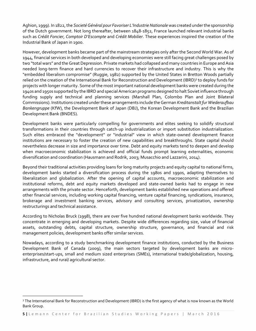
Aghion, 1999). In 1822, the Societé Général pour Favoriser L’Industrie Nationale was created under the sponsorship of the Dutch government. Not long thereafter, between 1848-1852, France launched relevant industrial banks such as Crédit Foncier, Comptoir D’Escompte and Crédit Mobilier. These experiences inspired the creation of the Industrial Bank of Japan in 1900.
However, development banks became part of the mainstream strategies only after the Second World War. As of 1944, financial services in both developed and developing economies were still facing great challenges posed by two “total wars” and the Great Depression. Private markets had collapsed and many countries in Europe and Asia needed long-term finance and hard currencies to recover their infrastructure and industry. This is why the “embedded liberalism compromise” (Ruggie, 1982) supported by the United States in Bretton Woods partially relied on the creation of the International Bank for Reconstruction and Development (IBRD)3 to deploy funds for projects with longer maturity. Some of the most important national development banks were created during the 1940s and 1950s supported by the IBRD and special American programs designed to halt Soviet influence through funding supply and technical and planning services (Marshall Plan, Colombo Plan and Joint Bilateral Commissions). Institutions created under these arrangements include the German Kreditanstalt fur Wiederaufbau Bankengruppe (KfW), the Development Bank of Japan (DBJ), the Korean Development Bank and the Brazilian Development Bank (BNDES).
Development banks were particularly compelling for governments and elites seeking to solidify structural transformations in their countries through catch-up industrialization or import substitution industrialization. Such elites embraced the “development” or “industrial” view in which state-owned development finance institutions are necessary to foster the creation of new capabilities and breakthroughs. State capital should nevertheless decrease in size and importance over time. Debt and equity markets tend to deepen and develop when macroeconomic stabilization is achieved and official funds prompt learning externalities, economic diversification and coordination (Hausmann and Rodrik, 2003; Musacchio and Lazzarini, 2014).
Beyond their traditional activities providing loans for long maturity projects and equity capital to national firms, development banks started a diversification process during the 1980s and 1990s, adapting themselves to liberalization and globalization. After the opening of capital accounts, macroeconomic stabilization and institutional reforms, debt and equity markets developed and state-owned banks had to engage in new arrangements with the private sector. Henceforth, development banks established new operations and offered other financial services, including working capital financing, venture capital financing, syndications, insurance, brokerage and investment banking services, advisory and consulting services, privatization, ownership restructurings and technical assistance.
According to Nicholas Bruck (1998), there are over five hundred national development banks worldwide. They concentrate in emerging and developing markets. Despite wide differences regarding size, value of financial assets, outstanding debts, capital structure, ownership structure, governance, and financial and risk management policies, development banks offer similar services.
Nowadays, according to a study benchmarking development finance institutions, conducted by the Business Development Bank of Canada (2009), the main sectors targeted by development banks are micro-enterprises/start-ups, small and medium sized enterprises (SMEs), international trade/globalization, housing, infrastructure, and rural/ agricultural sector.
3 The International Bank for Reconstruction and Development (IBRD) is the first agency of what is now known as the World Bank Group.

6 | L e m a n n C e n t e r f o r B r a z i l i a n S t u d i e s W o r k i n g P a p e r s | M a r c h 2 0 1 6
Currently, important development banks include national and multilateral entities (Table 1).
Table 1: Development Banks, USD million (2013)
Total Assets
Total Loans
Debt Ratio
D/E Ratio
NIM ROA ROE
National Development Banks
China Development Bank 1,352,844 1,181,065 0.93 13.57 0.02% 1.02% 15.07%
German Development Bank (KfW)
640,850 159,566 0.95 21.67 0.56% 0.26% 6.57%
BNDES 332,228 121,673 0.91 11.20 1.54% 1.02% 12.85%
Korean Development Bank
159,305 94,917 0.88 7.94 0.02% -0.98% -8.80%
Development Bank of Japan
158,248 147,987 0.84 5.40 0.00% 0.51% 2.86%
Multilateral Development Banks
IBRD 325,601 143,667 0.87 7.23 1.58% 0.06% 0.55%
Asian Development Bank 115,868 53,088 0.85 5.76 1.16% 0.48% 3.37%
IDB 97,007 70,782 0.77 3.11 2.03% 1.34% 5.54%
Source: Author’s elaboration based on data from Banks’ annual reports and Bloomberg
3. Brazilian National Development Bank (BNDES)
Brazil started major transformations in its productive structure just after the outbreak of the Great Depression. Manufacturing sectors such as perishable and semi-durable goods surged in the 1930s and 1940s. Bilateral agreements between Brazil and the United States created an agenda for the development of industrial projects during the Second World War. Under the so-called “Washington Accords,” the United States provided technical assistance and financing for strategic capital-intensive projects, including a big steelworks company (CSN) and a large-scale iron ore mining enterprise (Vale do Rio Doce). Moreover, the American Technical Mission (Cooke Mission) conducted the first comprehensive study diagnosing the Brazilian economy, recommending sectorial development of transport, fuel, textiles, minerals, chemicals, and education.
However, the war also imposed a scarcity of inputs for both infrastructure and industry in Brazil, causing a depreciation of fixed capital stocks. Hence, after the US released its programs to support economic reconstruction in Europe and Asia, Brazil asked for technical and financial cooperation in similar terms. Washington answered creating the Brazil-United States Technical Commission (Abbink Mission) and the Joint Brazil-United States Development Commission (CMBEU). While the Abbink Mission designed the first draft of a development plan for Brazil, outlining several investment projects, the CMBEU developed a “bottleneck” approach to prioritize investments. In addition, the CMBEU conducted feasibility studies for the projects, infusing planning, project development and project management technology in Brazil.
CMBEU and the National Plan for Economic Renovation considered infrastructure depreciation as the main bottleneck preventing industrial development. Thus, most of the 41 projects suggested by the CMBEU were either energy or transport related. Resources for project development were to be granted by the IBRD and American Export-Import Bank. In order to have access to these loans and grants, Brazil had to mobilize resources to supply projects with local currency. A modern mechanism for large-scale capital mobilization had to be developed. Industrial projects could not rely only on non-recoverable loans from the national budget, and no one would be willing to voluntarily lend long-term because of inflation and macroeconomic instability. Thus, the government opted to create compulsory savings (i.e., involuntary contribution of firms, workers, consumers and individuals for saving funds managed by public institutions). As of 1952, the Fund for Economic Renovation (FRE)

7 | L e m a n n C e n t e r f o r B r a z i l i a n S t u d i e s W o r k i n g P a p e r s | M a r c h 2 0 1 6
was established, receiving compulsory loans from a 15% extra fee to income tax, a compulsory collection of 4% of all deposits from the Federal Housing Bank and of 25% of technical reserves from insurance and capitalization companies (BNDES, 2002).
FRE was nevertheless unable to undertake infrastructure and industrial projects without additional expertise and administrative support. Therefore, the CMBEU suggested that a development bank should be founded to intermediate and manage resources mobilized for the investment projects and programs. The Brazilian Development Bank (BNDES)4 was hence created as a development finance device applying the most up-to-date technics available for project preparation, appraisal, financing, implementation and evaluation.
International funding from the IBRD and the Export Import Bank were canceled after the rise of Dwight Eisenhower to power in the US and the nationalistic path taken by president Getulio Vargas in the end of his second government (1950-54). From 1952 until 1966, funding for the BNDES mostly came from the FRE (32%) and from restricted funds created to foment specific sectors such as electricity, railways, capital goods and equipment. During this period, the BNDES focused its operations in a small number of big projects, including hydroelectric power stations, transmission lines and steelworks, being an agent for the “big push” (“50 years in 5”) conducted by the Target Plan of president Juscelino Kubitschek (1955-60).
Political instability and the lack of strong democratic institutions facilitated the implementation of a military dictatorship in 1964. Two years later, compulsory savings for the FRE ceased and the BNDES had to struggle to mobilize funds from the fiscal budget and monetary reserves. Activities were nevertheless kept and the BNDES relied on restricted funds to diversify its portfolio. During this period, support for private projects prevailed over public projects because restricted funds for infrastructure were reallocated to state-owned companies such as the Federal Railway Network S.A., the Brazilian Hydroelectric Centers S.A. (Eletrobras) and the Brazilian Steel S.A. (Siderbras). From 1964 until 1967, 43% of the USD 1.3 billion funding of the BNDES came from restricted funds, with the Fund for Industrial Plant and Machinery Financing (Finame) being the most relevant (Prochnik, 1995; BNDES, 1966-72).
Despite low annual real growth rates of GDP in 1964-67, stabilization and banking and capital market reforms conducted by finance minister Otávio Gouveia de Bulhões, planning minister Roberto Campos and central bank governor Mario Henrique Simonsen set the conditions for an economic modernization and expansion. Under these reforms, the experience of BNDES with long-term financing was important for the indexing of financial instruments. The mechanism was essential because government bond indexation allowed noninflationary financing of the budget deficit (BNDES, 2002).
Starting in 1968, Brazil underwent an economic boom known as the “Brazilian miracle” (1968-72), during which the GDP annual growth rate averaged 11.3% (Baer, 2014). Even after the oil shock of 1973 Brazil was able to push economic growth through the Second National Development Plan (IIPND) of president Ernesto Geisel. From 1973 until 1979, average annual GDP grew 6.8% (IBGE, 2003). BNDES was important for this outcome. During the “miracle,” disbursements from the BNDES reached USD 2.6 billion, a great amount compared to the USD 988 millions of total disbursements in 1952-68. In other words, annual disbursements averaged USD 520 million during the “miracle” and USD 58 million during the previous period. Annual disbursements from the BNDES averaged an increase of 48% per year in 1968-72.
By 1971, the consulting company Booz Allen Hamilton advised Brazilian authorities on administrative reform aiming to transform the BNDES’ governance and structure. In order to guarantee more independence and flexibility for the BNDES, the reform established its transition from a public agency to a state-owned company. Moreover, a new funding policy permitted the continuity of the expansion of BNDES after 1973. Instead of relying only on restricted funds, fiscal budget and monetary reserves, the BNDES gained access to compulsory savings from firms through the newly established Social Integration Program and Public Employee Savings Program
4 BNDES is the Portuguese acronym for Banco Nacional de Desenvolvimento Econômico e Social.

8 | L e m a n n C e n t e r f o r B r a z i l i a n S t u d i e s W o r k i n g P a p e r s | M a r c h 2 0 1 6
(PIS-PASEP). From 1974 until 1979, funds from PIS-PASEP accumulated USD 9.4 billion, helping to support disbursements of USD 20 billion and sustain an average increase in disbursements of 33% per year. Additionally, during this period, the BNDES created three subsidiaries—Embramec, Fibase and Ibrasa—to intervene in the capital markets, taking minority equity positions in companies deemed strategic for the national development.
BNDES was in fact the main agent behind the import substitution policies designed by president Geisel for sectors such as capital goods and basic inputs. Thus, the BNDES undertook major projects in steel, paper and pulp, petrochemicals, caustic soda, tin, zinc and aluminum, cement and fertilizer. However, everything was happening while the country’s foreign debt surged. External resources were important to fund gross capital formation, and net foreign debt increased at a yearly rate of 38.7% from USD 6.2 billion in 1973 to USD 31.6 billion in 1978. Furthermore, the share of public and publicly guaranteed debt of total medium- and long-term debt rose from 52% in 1973 to 63% in 1978 (Baer, 2014).
Two shocks led Brazilian rapid development to an abrupt end by the late 1970s and early 1980s: the second oil shock (doubling petroleum prices) and the US Federal Fund Rates hike (1000 basis points increase to 20%). Drastic movements affected the Brazilian current and capital accounts. Debt services increased from 30% of export earnings in 1974 to 83% in 1982. GDP growth rate plummeted to -4.5% in 1981. The “Lost Decade” loomed as the twilight of a long period of catch up and high GDP growth rates. From 1981 until 1990, nominal GDP growth averaged 1.6% yearly (IBGE, 2003). The Brazilian economy had to face a new age of fiscal crises, currency depreciation and high inflation. Adjustments became even more necessary in a period in which democratization and a new constitution added pressure on the fiscal budget.
BNDES had a fundamental role in this period, when most of the public agents and decision makers shortened their time horizons. Switching a sectorial approach based on individual projects to a method grounded on strategic planning, the BNDES crafted scenario analyses and changed its strategy accordingly. By 1984, the BNDES concluded that the age of state-led development was over. Under the “competitive integration” slogan, and based on a diagnostic pointing to the exhaustion of import substitution industrialization and public savings, the BNDES supported a new view about the role of the state, foreign capital and industrial policies (Mourão, 1994). Brazilian industry was no longer in “infancy.” Local entrepreneurs already had enough capacity to mobilize capital for complex projects, while state-owned companies were facing severe investment restrictions and political interferences.
By the beginning of the 1980s, dozens of companies that were originally private eventually fell under the BNDES control because of nonpayment of loans. Thus, the BNDES designed, organized and promoted the privatization of 14 companies in which it had equity majority. Moreover, the BNDES restructured its equity arm, unifying Embramec, Fibase and Ibrasa under a new subsidiary for capital market interventions called BNDES Participation (BNDESPAR).
Return on operations became the BNDES main funding source for the first time in 1981. Later on, the new Federal Constitution of 1988 established in its article number 239 that at least 40% of compulsory savings from PIS-PASEP should be channeled to BNDES for development finance, while the remaining 60% should finance the program for unemployment insurance and salary bonuses. As of 1990, with the Law Nº 7.998, savings from PIS-PASEP were unified under the Worker’s Assistance Fund (FAT).
Macroeconomic stability worsened in the end of the 1980s and the beginning of the 1990s. Hyperinflation and currency devaluation created economic chaos. The annual rate of inflation reached 2739% in 1990 and averaged 1400% between 1989 and 1994 (IBGE). Several economic plans failed one after another. Economic despair and political drama followed until the unleashing of the “Real Plan” in 1993 and 1994. Based on a de facto exchange-rate targeting regime (crawling peg), and benefiting from measures such as transparency, fiscal adjustment and a new indexing system, the Real Plan succeed in curbing hyper and very high inflation, paving the way for further economic modernization in Brazil.

9 | L e m a n n C e n t e r f o r B r a z i l i a n S t u d i e s W o r k i n g P a p e r s | M a r c h 2 0 1 6
4. Development Banking for Market Reforms
As of 1996, Brazilian yearly inflation measured by the internal general price index (IGP-DI) eased to one-digit figures for the first time since 1952 (IBGE). At first, price stability affected the so-called “inflation gains” of financial intermediaries in Brazil, demanding central bank intervention, new prudential regulations and government-sponsored devices for ownership restructuring (Studart, 2000; Baer and Nazmi, 2000). However, after the tapering of banking fragility, the Brazilian financial system was finally able to benefit from macroeconomic stabilization. Secondary capital markets developed and deepened, while investment and pension funds changed their strategy and portfolio, holding less short-term indexed bonds and estate assets and riskier positions. Under these conditions, new players loomed as potential or actual providers of long-term funds.
BNDES had an important role adapting itself and the Brazilian industry for the new economic momentum. Unlike other public agencies, the BNDES was aware of the exhaustion of the previous pattern of development financing and embraced economic reforms from the beginning. Therefore, the BNDES acted to “crowd in” private investments and develop capital markets, managing the famous National Privatization Program (PND). From 1990 to 2003, the BNDES directed 69 privatizations in sectors such as steel, chemical and petrochemical, fertilizers, electricity, rail transport, mining, ports, financial, and petroleum. Privatization included the transfer of control from government to the private sector and other operations such as concessions, leases and sales of minority stakes. Total results from the sale of companies, disposal of minority shares and concessions amounted to USD 39.7 billion (BNDES, 2003).
BNDES played three roles in the PND (Musacchio and Lazzarini, 2014):
(a) Operational agent of privatization transactions involving the sale of controlling blocks of state-owned companies;
(b) Financing provider for the buyers in some of the transactions; (c) Equity participation through its equity-holding arm, BNDESPAR.
During the 1990s and early 2000s, 86% of privatization revenues came from sales of controlling blocks, of which 53% were acquired by consortiums comprised of domestic groups, foreign investors and public entities such as the BNDESPAR and pension funds of state-owned companies. These include Previ (Banco do Brasil), Petros (Petrobras) and Funcef (Caixa Economica Federal) (Anuatti-Neto et al., 2005; Paula, 2002; Lazzarini, 2011).
Loans and equity capital from the BNDES were a sine qua non condition for a successful privatization program. Bids on controlling blocks in former state-owned companies would hardly reach minimum prices without a strong support from the BNDES and pension funds. Thus, the Brazilian state kept a strong presence in the economy even after privatization. According to Lazzarini (2011) and Musacchio and Lazzarini (2014), ownership restructurings in Brazil led to a decrease in the role of the state as a majority investor, but increased its power centrality5 and its position as a minority shareholder. Governmental entities, under the leadership of the BNDESPAR, ramped up their centrality in comparison to an average owner from 131% in 1996 to 553% in 2009. Similarly, pension funds from state-owned companies increase their centrality from 224% to 936% during the same period. In other words, the Brazilian state was able to boost its corporate influence by flexing the muscles of state-related entities holding dispersed stakes in several privatized, listed and non-listed companies.
Such arrangement also favored the development of financial services in Brazil. Few industries were as modernized as the banking industry. From 1995 to 2002, major changes affected the ownership structure of Brazilian banks. Private institutions supplied more credit than public institutions for the first time in 1999.
5 Power centrality or Bonacich centrality refers to the direct and indirect laces linking agents in a given network. In this case, the ownership networks in Brazil. Different connection degrees or centrality implies influence inequality among owners within a network. Centrality is therein the degree to which a group of owners distance themselves from the average connectivity of owners within the network.

10 | L e m a n n C e n t e r f o r B r a z i l i a n S t u d i e s W o r k i n g P a p e r s | M a r c h 2 0 1 6
Moreover, foreign banks increased their operations in this period, mostly after acquiring banks previously owned by state governments.
Figure 1: Share of Credit Operations by Bank Ownership, 1995-2002
Source: Author’s elaboration based on data from the Central Bank of Brazil
A balance of payment crises following the external shocks coming from Asia (1997) and Russia (1998) led Brazilian authorities to conduct a transition from the exchange-rate targeting regime to a inflation-targeting regime in 1999. Crawling peg to the dollar was abandoned and the new floating exchange rate required a new nominal anchor. The macroeconomic regime was thus grounded on a tripod including a (i) target inflation rate, a (ii) target primary surplus to reduce the debt-to-GDP ratio, and a (iii) floating exchange rate. Communication and accountability became vital (Bogdanski et al., 2000), and new policies enhanced credibility and favored a stronger external position. Such endeavors improved Brazilian fiscal position and helped to drastically reduce inflation volatility (Segura-Ubiergo, 2012).
The macroeconomic tripod including its inflation-targeting regime persisted even after the substitution of President Fernando Henrique Cardoso’s Social-Democratic Party (PSDB) with the left-leaning Worker’s Party (PT) of president Luiz Inacio Lula da Silva in 2003. The new macroeconomic model was indeed furthered during the first term of President Lula (2003-2006). Lower levels of inflation and inflation volatility allowed real interest rates to plunge from an average of about 20% during the exchange-rate targeting regime to an annual average of about 10% during 2000-2005 and to below 8% between 2006 and 2009 (Segura-Ubiergo, 2012). Expectations over inflation and interest rates were tamed by the central bank (Bevilaqua et al., 2007), fostering the development of capital and debt markets. Stock markets boomed, attracting new entrepreneurs, promoting better practices of corporate governance and enlarging the investor base.
Figure 2: Market Capitalization of Listed Companies in Brazil, 1995-2011
Source: Author’s elaboration based on data from the World Development Indicators
0%
20%
40%
60%
80%
0%
20%
40%
60%
80%
1995 1996 1997 1998 1999 2001 2002
Public Banks
Private Banks
0.00%
20.00%
40.00%
60.00%
80.00%
100.00%
120.00%
0
500
1000
1500
2000
Market Capitalization ofListed Companies (USDBillion)
Market Capitalization ofListed Companies (% ofGDP)

11 | L e m a n n C e n t e r f o r B r a z i l i a n S t u d i e s W o r k i n g P a p e r s | M a r c h 2 0 1 6
5. Development Banking in the Post-Crises Blues
Despite structural reforms and relevant improvements in the macroeconomic setting, the Brazilian sovereign yield curves in domestic currency are persistently volatile and high, preventing private agents from borrowing long-term and blocking the development of a free market for long-term credit at fixed interest rates in Brazilian Reais (BRL) (Sotelino, 2014).
Moreover, real interest rates are much higher in Brazil than in other emerging and developing markets. While short-term real interest rate is 5.64% in Brazil, other BRICS and MINT countries benefit from far better rates, including 4.10% for China, 3.60% for Russia, 2.75% for India, 1.06% for Indonesia, 0.51% for Turkey, 0.45% for South Africa and -1.08% for Mexico (Trading Economics).6
Figure 3: Brazilian Sovereign Yield Curve, LFT, LTN and NTN-F (Selic-based and fixed-rate bonds)
Source: Author’s elaboration based on data from the Central Bank of Brazil and National Treasury
This is a major problem for the sustainable development of capital markets in Brazil. Monetary stability and low rate risks increase the demand for long-term debts. Longer debt duration implies higher confidence and creditability, fostering the creation of benchmarks for debt markets and the widespread use of long-term commercial papers. High and volatile real interest rates express how the institutional construction of Brazilian stability is still incomplete (Lopes 2010).
Structural distortions such as the very short-term structure of debt stocks and country-specific factors related to credit market segmentation diminish the effectiveness of monetary policy. Having access to cheap funds based on compulsory savings arrangements, state-owned banks are able to supply credit at better-than-market terms, presenting less sensitivity to movements of the overnight market rate on federal debt repos (SELIC).
BNDES pays the so-called Long-Term Interest Rates (TJLP)7 for most of its funds.8 Being much lower and much less volatile than SELIC (Chart IV), the TJLP is the cornerstone of long-term financing in Brazil. Although it helps
6 February 5th, 2015. 7 A reference rate set quarterly by the Brazilian Monetary Council. 8 Debt with FAT-Constitutional is subordinated or quasi-equity. No amortizations are made while interests are paid semi-annually. Interests are limited to 6% per year for the TJLP liabilities. The excess yield is capitalized and added to the outstanding balance of FAT funds. Special Deposits FAT is comprised of additional resources channeled to the bank when
0.00%
5.00%
10.00%
15.00%
20.00%
25.00%
0 1 2 3 6 8 10
Years

12 | L e m a n n C e n t e r f o r B r a z i l i a n S t u d i e s W o r k i n g P a p e r s | M a r c h 2 0 1 6
to provide cheaper funding for entrepreneurs, it also lessens the power of monetary policy. Thus, along with the subsidized loans from Banco do Brasil and Caixa Economica Federal for housing and agriculture, the BNDES disbursements push upwards the equilibrium real interest rate in the free market (Segura-Ubiergo, 2012; Lopes, 2010; Bacha, 2010; Lara Resende, 2013).
Figure 4: Monthly rates of SELIC and TJLP (%), 2002-2015
Source: Author’s elaboration based on data from the BNDES and Central Bank of Brazil
However, the FAT—the only steady external source of funds for the BNDES—is depleting, which poses challenges for the future expansion of BNDES’ operations. The annual average of total net inflows from FAT as a share of total disbursements decreased from 14% in 2000-06 to 4.5% in 2007-14. Although net inflows from FAT-Constitutional are keeping pace with disbursements, higher minimum wages and increasing employment formalization are ramping up FAT annual expenditures with unemployment insurance, pushing FAT-Special Deposits net balance to negative levels and reducing total net inflows from FAT to the BNDES. FAT-Special Deposits net balance deteriorated quickly, plummeting from a positive amount of BRL 20 billion in 2000-06 to a negative amount of BRL 7.1 billion in 2007-14.
Figure 5: Net Inflows from FAT and Total Disbursements, 2000-2013
Source: Author’s elaboration based on data from BNDES’ annual reports
revenues from FAT exceed annual expenditures required by the legislation. BNDES’ USD-related liabilities pay USD LIBOR flat.
0.00
5.00
10.00
15.00
20.00
25.00
30.00
35.00
40.00
45.00
2002 2003 2004 2005 2006 2007 2008 2009 2010 2011 2012 2013 2014 2015
SELIC
TJLP
0.00%
5.00%
10.00%
15.00%
20.00%
25.00%
0
20
40
60
80
100
120
140
160
180
200
20
00
20
01
20
02
20
03
20
04
20
05
20
06
20
07
20
08
20
09
20
10
20
11
20
12
20
13
Total Disbursements, BRLBillion
Total Net Inflows fromFAT/ Disbursements

13 | L e m a n n C e n t e r f o r B r a z i l i a n S t u d i e s W o r k i n g P a p e r s | M a r c h 2 0 1 6
Net outflows from FAT-Special Deposits started amidst a surge in total disbursements. The gap was nevertheless more than fulfilled by resource mobilization from the National Treasury. From 2002 through 2014, the National Treasury funded the BNDES with BRL 426 billion. BNDES capital structure thus changed accordingly, with the participation of the National Treasury increasing from BRL 3.8 billion or 3.4% of total in 2001 to BRL 450 billion or 54% of total in 2014. FAT relative participation in the capital structure decreased from BRL 69.4 billion or 61.5% of total to BRL 192.4 billion or 23% of total during the same period.
Reasons behind government support of the BNDES include anti-cyclical policies after the subprime meltdown of 2007 and credit crunch of 2008, a renewal bet on industrial policies “picking winners” and fostering “national champions,” and progressive changes on macroeconomic policies leading to the so-called “new economic matrix” of president Dilma Rousseff. New government bonds were issued by the National Treasury to channel funds to the BNDES. Differences between government borrowing costs and subsidized TJLP imply resource mobilization from the National Treasury to the BNDES have a fiscal impact, affecting the gross national debt and crowding out private investment.
From 2004 to 2014, BNDES’ total assets increased over five-fold in BRL and over six-fold in USD to BRL 834,756 million or USD 356,733 million in 2014 (Figure 6). Similarly, BNDES disbursements ramped up over four-fold in BRL and over five fold in USD to BRL 187 billion or USD 80 billion in 2014 (Figure 7).
Figure 6: Total Assets, 2004-2014
Source: Authors’ elaboration based on BNDES and IPEA data
0
100,000
200,000
300,000
400,000
500,000
600,000
700,000
800,000
900,000
2004 2005 2006 2007 2008 2009 2010 2011 2012 2013 2014
BRL USD

14 | L e m a n n C e n t e r f o r B r a z i l i a n S t u d i e s W o r k i n g P a p e r s | M a r c h 2 0 1 6
Figure 7: BNDES Disbursements, 2004-2014
Source: Authors’ elaboration based on BNDES and IPEA data
Expansion in earmarked loans attained remarkable success preventing a credit crunch and a recession in Brazil; however, the macro, industrial and social views prevailing in the government pushed for a continuing mobilization of funds even after the economy fully recovered. Out of the BRL 413 billion raised by the National Treasury to the BNDES since the beginning of the international financial crisis in 2007, BRL 283 billion or 66% was raised after 2009, when the Brazilian economy rebounded strongly. The new matrix of Brazilian economic policies boosted government-driven credit expansion, which ramped up participation of state-owned banks in the national credit market.
Figure 8: Share of Credit Operations by Bank Ownership, 2002-2013
Source: Authors’ elaboration based on data from the Central Bank of Brazil
0
20
40
60
80
100
120
140
160
180
200
2004 2005 2006 2007 2008 2009 2010 2011 2012 2013 2014
BRL USD
0%
10%
20%
30%
40%
50%
60%
70%
80%
0%
10%
20%
30%
40%
50%
60%
2002 2003 2004 2005 2006 2007 2008 2009 2010 2011 2012 2013
Public Banks
Private Banks

15 | L e m a n n C e n t e r f o r B r a z i l i a n S t u d i e s W o r k i n g P a p e r s | M a r c h 2 0 1 6
During this period, BNDES surpassed Santander and consolidated its position as the fifth largest bank by total assets and total loans in Brazil (Table 2).
Table 2: Largest Banks in Brazil, BRL million (2013)
Total Assets
Total Loans Debt Ratio
D/E Ratio NIM ROA ROE
Banco do Brasil 1,437,485 645,674 0.41 6.87 3.93% 1.20% 21.88%
Itau Unibanco 1,105,721 412,234 0.37 5.05 4.77% 1.52% 20%
Caixa Economica Federal
858,325 485,487 0.43 10.24 2.81% 0.86% 22.63%
Bradesco 838,301 323,979 0.4 4.67 4.84% 1.45% 16.92%
BNDES 784,857 287,148 0.91 11.20 1.54% 1.02% 12.85%
Santander Brasil 453,052 226,206 0.35 3.55 5.68% 1.18% 7.03%
Safra 124,399 48,662 0.59 10.34 4.21% 1.09% 19.09%
BTG Pactual 120,888 18,119 0.16 1.55 7.32% 2.29% 21.65%
Source: Author’s elaboration based on data from banks’ annual reports and Bloomberg
Holding a virtual monopolist position over long-term financing, BNDES channels subsidies from compulsory savings and Treasury transfers to its customers. BNDES’ net interest margin (NIM) was 1.54% in 2013, 325 basis points lower than the average of the eight largest banks in Brazil, 183 basis points lower than the average of the two biggest state-owned banks and 376 basis points lower than the average of the five largest private banks.
Yet, BNDES had a net income of BRL 8,150 million in 2013. However, gross income from loans registered a loss of BRL 1,649 million, being offset only by the BRL 11,271 million earned by returns on securities. It is worth noting that 72% of the BRL 160,829 million held by the BNDES in securities is state-related, including BRL 62,934 million in government and sovereign bonds and BRL 39,830 million in shares from state-owned companies. If subsidies for its funding were eliminated, BNDES’ net interest margin would drop from 1.54% to -4.37% in 2013. In other words, taxpayers spent over 4 cents for every dollar allocated by the BNDES during the year.
Subsidies are justified whenever government driven loans fulfill market failures, funding projects that cannot be funded by private markets but whose social benefits exceeds their financial costs. This includes credit to capital constrained firms and social intensive sectors.9 However, recent empirical analyses and econometric studies strongly support that BNDES’ operations do not maximize social welfare (Bonomo et al., 2014; Lazzarini et al., 2015; Mello and Garcia, 2012; Sousa, 2010). BNDES channels 67% of its total disbursements to large enterprises that can fund their projects with other sources of capital. Moreover, such trends have strengthened after the international financial crisis and the surge on government driven credit. Recently, larger, older and less risky firms benefited most from government-sponsored loans. Monopolistic firms have 18% higher chances of receiving loans from the BNDES than other firms – chances were 11% higher before 2007. Additionally, BNDES reduced its relative participation in social intensive sectors by 25% after the international crisis (Bonomo et al., 2014).
Resources allocated to large “national champions” could still be justified if loans and equity capital had a positive effect on firms’ performance, investment or productivity, funding their riskier projects and boosting innovation. But data shows no significant effect of BNDES loans and equity capital on firms’ profitability, market valuation (Lazzarini et al., 2015), productivity (Sousa, 2010), investment and capital expenditures (Bonomo et al., 2014; Lazzarini et al., 2015). There is simply no evidence that services provided by the BNDES stimulate potential output growth. Rather, evidence suggests publicly listed firms are borrowing long-term to either reduce capital costs or even benefit from interest rate arbitrage profit (Bonomo et al., 2014).
9 Social intensive sectors can include infrastructure, education, health, housing and agriculture.

16 | L e m a n n C e n t e r f o r B r a z i l i a n S t u d i e s W o r k i n g P a p e r s | M a r c h 2 0 1 6
Thus, Brazil clearly needs to reform its development banking system. The national government can indeed undermine macroeconomic stability if it keeps using BNDES to artificially expand credit or to support para-fiscal policies and accounting gimmicks. Dilma’s new economic team is willing to reinforce the inflation target regime and implement fiscal discipline. Among other measures, the new team supports a slow down on government driven credit and smaller SELIC-TJLP spreads.
However, the BNDES needs deeper changes. Funding structure and implicit subsidies imply disbursements should support projects with higher social externalities. In this sense, BNDES targeting and selecting policies may follow the trend created by leading development finance institutions, increasing the share of social intensive projects in its portfolio. Priorities may include micro-enterprises and start-ups, small and medium sized enterprises (SMEs), infrastructure, and international trade. Project monitoring and control should be enhanced, subjecting firms to performance targets conditional on their allocated capital. Finally, given the structural limits of compulsory savings and macroeconomic restrictions to further Treasury transfers, the BNDES should improve its governance and rely more on market funding and private sources of savings and widen market-based operations and off-balance sheet activities such as syndications, co-finance operations, project finance and underwritings.
6. Conclusions
Firms based in emerging markets often face capital constraints and other restrictions because of market failures such as financial incompleteness, capital markets pro-cyclicality, risk-aversion and coordination problems. Hence, emerging markets have to foster development finance through public policy. Harnessing state-owned development banks became one of the most effective ways to provide long-term finance and boost industrialization after the Second World War. However, globalization, liberalization, stabilization and privatization raised many challenges for traditional development banking in the 1990s and mid-2000s. Good governance, transparency and market-based operations turned out to be even more essential for financial sustainability thereafter. To some extent, all development banks had to adapt to the new set of best practices.
BNDES is the third largest development bank by total assets and fifth largest by total loans. One of the cornerstones of the Brazilian “developmental state,” the BNDES funded the most important infrastructure and industrial projects of the 1950s, 1960s and 1970s, nourishing a catching up process that consolidated a large base of diversified private groups. Despite its protagonist role during the “golden years” of Brazilian style state capitalism, BNDES embraced economic reforms after the international debt crisis exhausted import substitution policies and public savings in the 1980s. Crowding in private investors and developing capital markets, the BNDES operated and managed the National Privatization Program (PND).
Along with the macroeconomic stabilization, the PND created conditions for further modernization. Paradoxically, although ownership restructurings diminished state participation as a majority investor, it boosted its corporate influence as a minority shareholder. Positions were held through BNDES’ equity arm BNDESPAR and state-related entities such as pension funds of state-owned companies. Thus, the government was able to increase its power centrality while major changes increased the performance of former state-owned companies, favoring the development and deepening of capital and credit markets.
However, the subprime meltdown of 2007 and the global credit crunch of 2008 blocked the ongoing process of capital market development in Brazil. Hence, the BNDES was used to boost a credit-driven anti-cyclical program. Disbursements increased three fold, while funds were mobilized through government bond emissions. Proponents of economic interventionist policies gained momentum and pushed for a continuing mobilization of funds even after the economy fully recovered. Thus, selection problems increased and earmarked loans became less efficient.
Following these endeavors, Brazil now needs to reform its development banking system. BNDES funding structure and implicit subsidies imply disbursements should support projects with higher social externalities. In

17 | L e m a n n C e n t e r f o r B r a z i l i a n S t u d i e s W o r k i n g P a p e r s | M a r c h 2 0 1 6
this sense, targeting and selecting policies may follow the trend created by leading development finance institutions, increasing the share of social intensive projects in its portfolio. Finally, given the structural limits of compulsory savings and macroeconomic restrictions to further Treasury transfers, the BNDES should improve its governance and rely more on market funding and private sources of savings and widen market-based operations and off-balance sheet activities such as co-finance operations, project finance and underwritings.
References Cited
ARMENDÁRIZ DE AGHION, B. (1999): “Development Banking” Journal of Development Economics 58(1), pp. 83-100.
BACHA, E. (2010): “Alem da Triade: Ha como reduzir os juros?”, Working Paper Nº 17, Instituto de Estudos de Politica Economica Casa das Garças, Rio de Janeiro, Brazil.
BAER, W. (2014): The Brazilian Economy: Growth and development. Boulder, CO: Lynne Rienner Publishers. BAER, W. and NAZMI, N. (2000): “Privatization and Restructuring of Banks in Brazil” The Quarterly Review of
Economics and Finance 40(1), pp. 3-24. BNDES (2012): BNDES: Um banco de histórias e do futuro. Rio de Janeiro: BNDES. BNDES (1995/2014): Individual and Consolidated Financial Statements. Rio de Janeiro: BNDES. BNDES (1966/1994): Relatorios de Atividade. Rio de Janeiro: BNDES. BEVILAQUA, A., MESQUITA, M. and MINELLA, A. (2007): “Brazil: Taming inflation expectations”, Working Paper
Nº 129, Banco Central do Brasil, Rio de Janeiro. BOGDANSKI, J., TOMBINI, A. and WERLANG, S. (2000): “Implementing Inflation Targeting in Brazil”, Working
Paper Nº 1, Banco Central do Brasil, Rio de Janeiro. BONOMO, M., BRITO, R. and MARTINS, B. (2014): “Macroeconomic and Financial Consequences of the After
Crisis Government-Driven Credit Expansion in Brazil”, Working Paper Nº 378, Banco Central do Brasil, Rio de Janeiro.
BRUCK, N. (1998): “The Role of Development Banks in the Twentieth-First Century” Journal of Emerging Markets 3(3), pp. 61-90.
CAMERON, R. (1961): France and the Economic Development of Europe. Princeton, NJ: Princeton University Press.
CÉSPEDES, L.F., CHANG, R. and VELASCO, A. (2002): “IS-LM-BP in the Pampas”, Working Paper Nº 9337, National Bureau of Economic Research, Cambridge, MA.
DEWATRIPONT, M. and MASKIN, E. (1995): “Credit and Efficiency in Centralized and Decentralized Economies” Review of Economic Studies 62(4), pp. 541-555.
DIAMOND, D. (1984): “Financial Intermediation and Delegated Monitoring” Review of Economic Studies 51(3), pp. 393-414.
EICHENGREEN, B. and HAUSMANN, R. (1999): “Exchange Rates and Financial Fragility”, Working Paper Nº 7418, National Bureau of Economic Research, Cambridge, MA.
EICHENGREEN, B., HAUSMANN, R. and PANIZZA, U. (2002): “Original Sin: The pain, the mystery, and the road to redemption”, In Inter-American Development Bank Conference, Washington, DC, 21-22 November.
GERSCHENKRON, A. (1962): Economic Backwardness in Historical Perspective. Cambridge, MA: Harvard University Press.
HAUSMANN, R. and RODRIK, D. (2003): “Economic Development as Self-Discovery” Journal of Development Economics 72(2), pp. 603-633.
HIRSCHMAN, A. (1958): The Strategy of Economic Development. London: Oxford University Press. IBGE (2003): Estatisticas do Seculo XX. Rio de Janeiro: IBGE. LA PORTA, R., LOPEZ-DE-SILANES, F. and SHLEIFER, A. (2002): “Government Ownership of Banks” The Journal
of Finance 52(1), pp. 265-301. LAZZARINI, S., MUSACCHIO, A., MELLO, R. and MARCON, R. (2015): “What Do State-Owned Development
Banks Do? Evidence from BNDES, 2002-09” World Development 66, pp. 237-253. LAZZARINI, S. (2011): Capitalismo de Laços: Os donos do Brasil e suas conexoes. Rio de Janeiro: Elsevier.

18 | L e m a n n C e n t e r f o r B r a z i l i a n S t u d i e s W o r k i n g P a p e r s | M a r c h 2 0 1 6
LEVY-YEYATI, E., MICCO, A. and PANIZZA, U. (2004): “Should the Government Be in the Banking Business? The role of state-owned and development banks”, In Governments and Banks: Responsibilities and Limits, Inter-American Development Bank, Lima, Peru, March 28.
LOPES, F. (2010): “A Estabilização Incompleta”, Working Paper, Macrometrica, Rio de Janeiro. MAZZUCATO, M. (2013): The Entrepreneurial State. London: Anthem Press. MELLO, J., and GARCIA, M. (2012): “Bye, Bye Financial Repression, Hello Financial Deepening: The anatomy of
a financial boom” The Quarterly Review of Economics and Finance 52(2), pp. 135-153. MOURAO, J. (1994): “A Integração Competitiva e o Planejamento Estratégico no Sistema BNDES” Revista do
BNDES 1(2), pp. 3-26. MUSACCHIO, A. and LAZZARINI, S. (2014): Reinventing State Capitalism: Leviathan in business, Brazil and
beyond. Cambridge, MA: Harvard University Press. OCAMPO, J.A. (2013): “Balance of Payments Dominance: Its implications for macroeconomic policy”, Initiative
for Policy Dialogue Working Paper Series, New York, NY. OCAMPO, J.A., RADA, C. and TAYLOR, L. (2009): Growth and Policy in Developing Countries: A structuralist
approach. New York, NY: Columbia University Press. OCAMPO, J.A. (2003): Capital Account and Counter-Cyclical Prudential Regulations in Developing Countries, In
French-Davis, R. and Griffith-Jones, S. (eds.): From Capital Surges to Drought: Seeking stability for emerging markets. London: Palgrave Macmillan.
PREBISCH, R. (1948): “The Economic Development of Latin America and Its Principal Problems” Economic Survey of Latin America 11, United Nations, New York, NY.
PROCHNIK, M. and MACHADO, V. (2008): “Fontes de Recursos do BNDES” Revista do BNDES 14(29), pp. 3-34. PROCHNIK, M. (1995): “Fontes de Recursos do BNDES” Revista do BNDES 2(4), pp. 143-180. RESENDE, A. (2013): Os Limites do Possível: A economia além da conjuntura. Sao Paulo: Penguin. RODRIK, D. (2004): “Industrial Policy for the Twenty-First Century”, John F. Kennedy School of Government
Paper, Harvard University, Cambridge, MA. RODRIK, D. (2007): “Normalizing Industrial Policy”, John F. Kennedy School of Government Paper, Harvard
University, Cambridge, MA. ROSESTEIN-RODAN, P. (1943): “Problems of Industrialization of Eastern and South-Eastern Europe” The
Economic Journal 53(211), pp. 202-211. RUGGIE, J. (1982): “International Regimes, Transactions, and Change: Embedded liberalism in the postwar
economic order” International Organization 36(2), pp. 379-415. SAYERS, R. (1957): Central Banking After Bagehot. Oxford: Oxford University Press. SEGURA-UBIERGO, A. (2012): “The Puzzle of Brazil’s High Interest Rates”, Working Paper Nº 12/62, IMF,
Washington, DC. SOTELINO, F. (2014): “A Functional Financial System for Brazil, When?”, In BRICS Lab Conference: BRICS, the
road ahead, Columbia University, New York, NY, 6 March. STIGLITZ, J. (1994): “The Role of the State in Financial Markets”, In Proceedings of the World Bank Annual
Conference on Economic Development, Washington, DC. STUDART, R. (2000): “Financial Opening and Deregulation in Brazil in the 1990s: Moving towards a new pattern
of development financing?” The Quarterly Review of Economics and Finance 40(1), pp. 25-44.

19 | L e m a n n C e n t e r f o r B r a z i l i a n S t u d i e s W o r k i n g P a p e r s | M a r c h 2 0 1 6
Fiscal Policy in Brazil: from Counter-Cyclical Response to Crisis
Márcio Holland10
Abstract: The main goal of this article is to identify the dynamic effects of fiscal policy on output in Brazil from
1997 to 2014, and, more specifically, to estimate those effects when the output falls below its potential level. To
do so, we estimate VAR (vector autoregressive) models to generate impulse-response functions and
causality/endogeneity tests. Our most notable results indicate the following channel of economic policy in Brazil:
to foster output, government spending increases causing increases in both tax rates and revenue and the short-
term interest rate. A fiscal stimulus via spending seems efficient for economic performance as well as monetary
policy; however, the latter operates pro-cyclically in the way we defined here, while the former is predominantly
countercyclical. As the monetary shock had a negative effect on GDP growth and GDP growth responded
positively to the fiscal shock, it seems that the economic policy has given poise to growth with one hand and
taken it with the other one. The monetary policy is only reacting to the fiscal stimuli. We were not able to find
any statistically significant response of the output to tax changes, but vice versa seems to work in the Brazilian
case.
1. Introduction
The 2008 international financial crisis put fiscal policy at the forefront of debate, particularly its use in mitigating the painful effects of the crisis on outputs and employment. Probably because of the lack of widely recognized rules, fiscal policy is generally a controversial issue. The economic meltdown with its deep and protracted impact on both goods and labor markets presented the perfect opportunity to approach divergent views about its use. For a few years after the 2008 crash, there was no room for austerity until government debts skyrocketed. Alas, governments had to shift towards fiscal retrenchment, even under economic weakness. The results of recent fiscal policies have been mixed, and their effectiveness remains a disputed issue.
On the other hand, a stream of literature has conducted empirical studies with novel methodologies in an effort to identify the dynamic and contemporaneous effects of fiscal policy on outputs. Auerbach and Gorodnichenko (2012) estimate a government purchase multiplier for a large number of OECD countries using a specific form of the STVAR (smooth transition vector autoregressive) model and have identified a fiscal multiplier in both recession and expansion circumstances. The model might be considered a refinement of Blanchard and Perotti’s (2002) specification, who used a simplified structural VAR model. In 2014, Mineshima et al. introduced a TVAR (threshold vector autoregressive) model to use when regimes are determined by a transition variable, which is either exogenous or endogenous. More recently, Herwartz and Lütkepohl (2014) proposed a structural vector autoregression model with Markov switching that combines conventional and statistical identification of shocks, which can be useful for future studies on fiscal policy.
The main goal of this article is to identify the effect of fiscal shocks on output in Brazil from 1997 to 2014, and, more specifically, to estimate those effects when the output falls below its potential level, as observed during most of the period following the 2008 international meltdown. We pose an additional question: How low can the
10 São Paulo School of Economics at Getulio Vargas Foundation, Brazil. Corresponding author contact: [email protected]. This working paper was partially written during my mandatory cooling-off period when I spent part of this time as a visiting scholar at Columbia University in the City of New York and for this reason I am very grateful to Professors Albert Fishlow, Thomas Trebat, Gray Newman, Sidney Nakahodo, Gustavo Azenha, and Daniella Diniz, for having me and giving me all the support I needed to develop my research. However, all opinions expressed herein represent those of the author.

20 | L e m a n n C e n t e r f o r B r a z i l i a n S t u d i e s W o r k i n g P a p e r s | M a r c h 2 0 1 6
output drop when it is already below its potential level (which we call “negative initial conditions” for the fiscal consolidation program), despite the composition of the fiscal retrenchment? In other words, after the output has bottomed out, how can policymakers quickly instill confidence by cutting expenditures and increasing taxes when these measures were supposed to be implemented as an expansionary shock?
To do so, we estimate VAR (vector autoregressive) models to generate impulse-response functions and causality tests. Our most notable results indicate the following channel of economic policy in Brazil: to foster output, government spending increases, causing increases in both tax rates and revenue and the short-term interest rate. A fiscal stimulus via spending seems quite efficient for economic performance as well as monetary policy; however, the latter operates pro-cyclically, while the former is predominantly countercyclical. We were not able to find any statistically significant response of the output to tax changes, but we did find a statistically significant response of tax changes to output in the Brazilian case.
The contributions of this work are threefold: first, it identifies the response of output to fiscal and monetary policy; second, it estimates the impact of recent fiscal measures on output; and, third, in line with broader economic literature, it suggests a long-term fiscal plan for Brazil to spur its effectiveness in reducing output losses.
This work is divided in the following sections. The next section shows Brazil’s recent experience with fiscal policy and its main results. The third section reviews the literature and discussions of the effectiveness of fiscal policy. The fourth section extrapolates the impulse-response functions obtained in our research to measure the potential impact of the 2015 fiscal plan on output and confidence. Ultimately, it is the appropriate moment to present the advantages and caveats of our empirical procedures. We are aware of the many drawbacks presented in this sort of time series analysis. At the end of this section, we suggest a long-term fiscal plan for Brazil using lessons learned from both Brazil’s recent experience with fiscal policy and our empirical study.
2. The Brazilian Context
Governments across the globe responded to the 2008 crisis with unprecedented expansionary actions in recent economic history. Monetary and fiscal countercyclical actions were implemented to both stymie the contamination of the international crisis in financial systems and to resume growth as soon as possible.
From 2008 to 2010, fiscal and monetary stimuli were overwhelmingly recommended. However, since 2010, the focus has shifted to fiscal consolidation in advanced economies. Since then, fiscal results have improved over the world, even though the debt-to-GDP ratios remain high compared with those before the crisis. More recently, the United States has outperformed the euro area, where calling for austerity appears to have fallen out of fashion again, as illustrated in the 2015 Greek case.
The fiscal front has deteriorated dramatically in many advanced economies with mixed and far from outstanding achievements. However, comparing the 1929 Great Depression with the 2008 Great Recession, Eichengreen (2015:2) reflects on these crises as follows: “as a result of this different response, unemployment in the United States peaked at 10 percent in 2010. Though this was still disturbingly high, it was far below the catastrophic 25 percent scaled in the Great Depression”.
Due to this thought, the Brazilian government took a series of countercyclical policies to protect the local economy from crumbling. These policies seemed to work well, at least until 2013. The worst of the crisis was absorbed without any major disruption in the Brazilian economic system. Most importantly, the economy resumed growth in the 2nd quarter of 2009; the unemployment rate did not spike; real wages continued to grow; and consumer and business confidence recovered very quickly. Nevertheless, after a period of recovery until 2013, the overall growth remained disappointing, particularly given the very rapid deterioration in 2014, the strong contraction in 2015, and uncertainty about 2016 performance.

21 | L e m a n n C e n t e r f o r B r a z i l i a n S t u d i e s W o r k i n g P a p e r s | M a r c h 2 0 1 6
From late 2014 to early 2015, Brazil launched a tight fiscal program. The pro-cyclical biased fiscal consolidation plan is presumably considered the only plausible policy stance when solvency became the issue rather than economic activity. In Brazil, the diagnosis and prescription have been far from divergent. However, as highlighted by Frankel (2012), “a pro-cyclical fiscal policy magnifies the severity of the business cycle”. This controversy motivated this research to assess whether such fiscal consolidation policies are expected to hurt GDP growth to a greater extent because the economy is already under contraction. Alternatively, would they spur confidence so that the drag on economic activity could be avoided?
There is no doubt that fiscal stimuli were needed at that challenging time, when the Brazilian economy was severely hit by the financial crisis. As for fiscal policy, there were considerable tax exemptions in 2009. As a result of the actions taken by the government at that time, the country was able to recover very quickly from the crisis; among other things, Brazil experienced 7.6 percent and 3.9 percent growth in 2010 and 2011, respectively (see table 1).
According to the national account’s new dataset, released on March 27, 2015 by the National Bureau of Statistics (IBGE), the 2008 crises hit the economy harder and deeper, and the recovery was faster and better because investment resumed quickly and included a greater share of the GDP compared with the previous period of the crisis, regardless of its volatility (see figure 1 and 2).
In early 2011, the Federal Administration was able to start applying a fiscal consolidation plan to cool down the economy. Needless to say, solvency had not been a problem in Brazil for a long time, as international reserves have been considerable and more than enough to pay for external liabilities; in addition, the public debt-to-GDP ratio had been decreasing over the years. Thanks to Brazil’s reaction to the crash, the general gross debt-to-GDP ratio increased 3.3% from 2008 to 2009, which could be considered incredibly low in comparison with the debt dynamics in advanced economies after the crisis. However, the general gross debt-to-GDP ratio is still high in Brazil compared with that of its peers, although it had been relatively stable, even during most of the period of countercyclical fiscal policy (see table 1 and figures 2 and 3 for the fiscal results).
Table 1. Brazil: Key Macroeconomic Indicators after the 2008 Crisis (2008-2015)
2008 2009 2010 2011 2012 2013 2014 2015* 2016*
Real GDP Change (%) 5,0 -0,2 7,6 3,9 1,8 2,7 0,1 -3,7 -3,0
Unemployment Rate year average (%)
7,9 8,1 6,7 6,0 5,5 5,4 4,8 6,8 7,5
Investment Change (%), eop 12,7 -1,9 17,8 6,6 -0,6 6,1 -4,4 -12,0 -5,0
CPI Inflation - IPCA (%), eop 5,9 4,3 5,9 6,5 5,8 5,9 6,4 -10,7 -8,5
Benchmark Interest Rate (%), eop 13,75 8,75 10,75 11,0 7,25 10,0 11,75 14,25 14,25
Current Account (% of GDP) -1,7 -1,5 -2,1 -2,0 -2,3 -3,4 -4,4 -4,5 -3,5
FDI (US$ billion) 45,1 25,9 48,5 66,7 65,3 64,0 96,9 60,0 50,0
Foreign Reserves (US$ billion) 207 239 289 352 379 376 374 370 360
Exchange Rate (Real per USD) eop 2,34 1,74 1,67 1,88 2,04 2,35 2,65 4,0 4,5
Primary Result (% of GDP) 3,3 1,9 2,6 2,9 2,2 1,8 -0,6 -1,9 -0,5
Nominal Result (% of GDP) -2,0 -3,2 -2,4 -2,6 -2,3 -3,1 -6,2 -10,3 -9,5
Gross G. Govt Debt (% of GDP) 56,0 59,3 51,8 51,3 54,8 53,3 58,9 66,2 72,0
Net Public Debt (% of GDP) 37,6 40,9 38,0 34,5 32,9 31,5 34,1 36 37,0
Notes: Unemployment rate is yearly average of the Monthly Employment Survey (PME); CPI is the broad CPI (IPCA); Benchmark interest rate is the target Central Bank interest rate in the end of period; and exchange rate as in the end of period. eop = end of period. * 2015 and 2016 are author´s forecasts. Source: Ministry of Finance of Brazil, Central Bank of Brazil, and IBGE.

22 | L e m a n n C e n t e r f o r B r a z i l i a n S t u d i e s W o r k i n g P a p e r s | M a r c h 2 0 1 6
Even with such policies, the primary surplus targets were fully accomplished, at least until 201211 (see figure 2). However, by mid-2012 to 2013, the recovery appeared to be weaker than expected, and the Brazilian economic authorities returned to incentives, trying to reignite the economy12. In 2013, the economy grew again by 2.7%, and the investment grew 6.1%. A wide tax relief program and increasing government expenditures, including a broad financial subsidy for credit for capital goods via public banks, were introduced. The economy reacted reasonably, so the investment to GDP ratio remained relatively stable at approximately 20.5% until at least 2013, despite its high variability (see figure 1).
Figure 1. Brazil: Gross Formation of Fixed Capital as % of GDP) 1997-2015
Source: IBGE, updated in November 17, 2015.
Note: Investment as % of GDP measured using current values for GDP and gross formation of fixed capital. 2015
is author´s forecast.
11 Although the one-off revenues had increased in importance after the 2008 crash, responding, for instance, to 0.74% and 0.85% of GDP in 2009 and 2010, respectively, when the full primary surplus delivered was 1.9% and 2.6% of GDP, respectively, or, in 2013, when 0.68% of 1.8% of GDP was one-off revenue. In 2014, one-off revenue was 0.5% of GDP while the primary deficit was 0.6% of GDP. 2015 primary surplus is going to be plenty of on-off revenue, as well. 12 At that time, estimates of GDP growth were 2.7% for 2011, instead of 3.9% as reported in the new 2015 dataset, moving downward towards 0.9% in 2012, instead of 1.8% as reported in the new 2015 dataset. Moreover, the share of investment over GDP was sharply declining, but the new 2015 dataset unveiled very stable figures for this indicator.
19.1
18.5
17.0
18.3 18.4
17.9
16.6
17.317.1 17.2
18.0
19.4
19.1
20.5 20.6 20.7 20.9
19.7 19.7
17.8
10.0
12.0
14.0
16.0
18.0
20.0
22.0

23 | L e m a n n C e n t e r f o r B r a z i l i a n S t u d i e s W o r k i n g P a p e r s | M a r c h 2 0 1 6
Figure 2: Nominal Fiscal and Primary Results as Share of GDP (%) 1999-2018
Source: Central Bank of Brazil; 2016 - 2018 are author´s forecast.
However, from 2013 to 2014, the output was not responding at all to tax stimuli or even spending increases. After Brazil graduated to respond to the 2008 crisis using countercyclical fiscal policies (Vègh and Vulletin, 2013), it experienced a rapid deterioration on the fiscal front in 2014. Both net and gross public debt increased quickly towards a risky case scenario, so the investment grade rating was no longer assured in the medium term13. Potential output decreased at the same time as the output was well below its declining potential output level.
In late 2014 and early 2015, some social benefits were reviewed, and some tax relief was reverted (tables 5.1 and 5.2 detail these measures). The economy had actually started to adjust itself during 2014, as the Central Bank had begun a new tightening cycle from April 2013 to July 2014. The target interest rate increased 375 basis points in an interval of one year. Another 325 basis-point increase would take place between October 2014 and July 2015. A 700 basis-point monetary shock in an interval of two years is far from negligible. Its primary side effect was a considerable contraction in the domestic credit on durable and capital goods, contributing to an additional drop in consumer and business confidence.
13 In September 2015, a couple of weeks after the Government had decided to send to Congress the 2016 Budget Law with deficit, the Standard & Poor´s downgraded the Brazilian sovereign rating to speculative grade.
(5.20)
(3.30) (3.30)
(4.40)
(5.20)
(2.90)
(3.50) (3.60)
(2.70)
(2.00)
(3.20)
(2.40) (2.50) (2.30)
(3.10)
(6.20)
(10,3)
(9.50)
(7.40)
(6.00)
2.80 3.20 3.30 3.20 3.20
3.70 3.70 3.20 3.20 3.30
1.90
2.60 2.90
2.20 1.80
(0.60)
(1,9)
(0.50)
0.50 1.00
(12.00)
(10.00)
(8.00)
(6.00)
(4.00)
(2.00)
-
2.00
4.00
6.00
1999 2000 2001 2002 2003 2004 2005 2006 2007 2008 2009 2010 2011 2012 2013 2014 2015 2016 2017 2018
Nominal Balance Primary Balance

24 | L e m a n n C e n t e r f o r B r a z i l i a n S t u d i e s W o r k i n g P a p e r s | M a r c h 2 0 1 6
Figure 3: Gross General Debt and Net Public Debt as Share of GDP (%) 2000-2018
Source: Central Bank of Brazil; 2016-2018 are author´s forecasts.
Since mid-2014 the Brazilian economy fell into full disarray: a combination of fiscal crisis with strong and prolonged GDP contraction in the midst of political chaos. There are many plausible explanations for the deceleration of the economy, including the monetary policy shock, associated curbing in household credit for durable goods, and the gradual increase in some tax rates. Meanwhile, the economy suffered from a myriad of other events, such as long-standing and severe drought, corruption scandals involving the largest Brazilian state-run oil company and major entrepreneurs in the civil construction sector, low government popularity amid street protests and general disapproval regarding the corruption scandals, several bribery schemes, and the 2014 FIFA World Cup. There are also drivers associated with a profounder phenomenon, as many analysts believe that the previous consumption-based growth model had already been exhausted. Unfavorable terms of trade are also remembered as another key driver of such exhaustion. However, I would highlight the exhaustion of domestic economic cycle as the main source of such difficulties, which could dramatize the GDP performance in coming years. Under this circumstance, the economy became very sensitive to either domestic or external shocks.
Therefore, fiscal results had been worsening faster than predicted, as the tax revenue had been frustrated in line with the growth downturn. Gross debt, as a percentage of the GDP, increased from 53.3% in December 2013 to 58.9% in December 2014 and, then, soared to 66% by December 2015. The gross debt prospects indicate further increases towards over 70% of GDP by the end of 2016 (see figure 3). In addition, surprisingly, the nominal deficit increased from 3.1 to 6.2% of GDP and skyrocketed to 10.3% of GDP in December 2015, a movement that was driven by interest payments, which also increased to 8.5% of GDP. Debt maturity and denomination have deteriorated with the same intensity.
As risks are tilted towards deep GDP contraction in 2015 and also in 2016, fiscal sustainability appears to have been an important issue yet again. For instance, in 2015, the net revenues of the central government decelerated -5.6% year-to-dates comparing to 2014. In that month, the government spending also declined -4.0%, in the same terms, although less than the tax frustration. Consequently, the rolling 12-month primary surplus of the central government decreased to -1,88% of GDP in 2015. Tax revenue frustration is only a partial explanation. In 2015, the government could not take into account the relevant amount of one-off revenues; and it also had to pay the delayed expenses, domestically labeled as “fiscal pedaling” (“pedalada fiscal”).
58.9
61.8
66.7
60.9
56.2 56.1 55.556.8 56.0
59.3
51.8 51.3
54.853.3
58.9
66.072.0
73.4
74.0
46.8
51.5
59.8
54.2
50.247.9
46.544.6
37.6
40.9
38.0
34.532.9
31.534.1
36.0 37.0 38.0
38.5
20.0
30.0
40.0
50.0
60.0
70.0
80.0
2000 2001 2002 2003 2004 2005 2006 2007 2008 2009 2010 2011 2012 2013 2014 2015 2016 2017 2018
Gross Debt (% GDP) Net Debt (% GDP)

25 | L e m a n n C e n t e r f o r B r a z i l i a n S t u d i e s W o r k i n g P a p e r s | M a r c h 2 0 1 6
Brazil fell into a severe fiscal crisis: the country failed to reach the required primary surpluses, that is, the level necessary to stabilize debt to GDP (this year and even in coming years). Therefore, the gross debt to GDP ratio is expected to soar 72% of GDP in 2016, from 53% of GDP, in 2013. This crisis is predicted to last many years. As far as I can tell, there is no solution, not even a light at the end of the tunnel.
The causes of such a fiscal situation are closely related to the causes of the GDP contraction. First, I would consider the stronger-than-expected GDP contraction that leads to tax revenue frustration even under tax rates hikes. It could also be explained by the growing government spending related to income transfer programs such as pension benefits14, LOAS15, Minha Casa Minha Vida (housing program), Bolsa-Família (a conditional cash transfer program), and etc. I would also include the reluctance in implementing the appropriate fiscal consolidation plan of early 2015. This hesitancy amplified the uncertainty on the economic recovery. Finally, because of the second round of the counter-cyclical fiscal policy implemented in 2012, delayed expenditures had to be settled during 2015. Meanwhile, intense realignment in the regulated price provoked a high short-term inflation. It seems there are many plausible explanations for such a drama experienced by the Brazilian economy like a perfect storm.
From a long-term perspective, as seen in figure 4, there has been a considerable change in government spending since 2003, as it has been focused on reducing poverty via increasing conditional cash transfer programs. The federal budget for education and housing has been increasing over the years. Total federal expenditures increased from 14.6% of GDP in 1997 to 18.6% of GDP at the end of 2014. Meanwhile, the net total federal tax revenue increased from 15.4% to 19.9% of GDP in 2010 and then decreased to 18.4% at the end of 2014. The recent fiscal stimuli combined to increase government expenditures by almost 1% of GDP, while the tax revenue declined from 19.8% to 18.4% of GDP. However, such recent efforts did not ignite growth in 2014. Many analysts question whether the overall fiscal multipliers decreased over this period of time. If so, why?
Figure 4. Brazil: Net Tax Revenue and Government Spending (% of GDP)1997-2016
Source: IBGE, and Ministry of Finance, Brazil. 2015 forecast according to the Minister of Planning.
14 The deficit in the general pension system is expected to reach 2.0% of GDP in 2016 from 1.0% of GDP in 2014. 15 LOAS is a welfare public policy for elderly with the benefits indexed to minimum wage. Its expenditure reached 0.7% of GDP, in 2014.
14.0
15.4
16.0 16.2
17.0
17.7
17.2
18.0
18.6 18.7 18.9 18.8
18.3
20.0
18.7 18.7
19.2
18.4 18.7
18.9
13.7
14.6
14.1 14.4
15.3 15.5
14.9
15.4
16.1
16.6 16.7
16.0
17.2
18.0
16.5
17.1 17.7
18.7
19.0 19.4
12.0
13.0
14.0
15.0
16.0
17.0
18.0
19.0
20.0
21.0
1997 1998 1999 2000 2001 2002 2003 2004 2005 2006 2007 2008 2009 2010 2011 2012 2013 2014 2015 2016
Net Tax Revenue (% GDP)
Primary Expenditure (% GDP)

26 | L e m a n n C e n t e r f o r B r a z i l i a n S t u d i e s W o r k i n g P a p e r s | M a r c h 2 0 1 6
So, what happened with the government expenditure over time? What are the main components of such increases? First of all, according to the table 2, the primary spending increased 2.8% of GDP since 2002, which is practically the same growth level of income transfers to households. Pension benefits show the most relevant increase followed by a welfare benefit for the elderly called LOAS. Part of the growth is related to both generous eligibility criteria and also public policy stance, due to the fact that the benefits are indexed to the minimum wage corrections.
As a matter of curiosity, because of this indexation rule, the benefits increased 78%, in real terms, in the last 10 years. At the same time, the number of beneficiaries increased by 9 million people, from 23 million to 32 million. Meanwhile, the government decided to enlarge social programs such as Bolsa Família and Minha Casa Minha Vida. Both are responsible for a 0.63% of GDP variation in the government consumption during this period of time.
Table 2. The Main Government Expenditure (2002-2014) % of GDP and Percentage Point (pp)
2002
(% GDP)
2010
(% GDP)
2014
(% GDP)
Variation
2002-2014 pp
Variation
2011-2014 pp
PRIMARY SPENDINGS 15,58 16,91 18,35 2,77 1,43
Payroll 4,77 4,28 3,98 -0,79 -0,30
Income Transfer to Households 6,51 8,25 9,31 2,79 1,05
Pension Benefits 5,90 6,56 7,14 1,24 0,58
Unemployment Insurance and Wage
Bonus 0,48 0,77 0,98 0,49 0,21
Welfare Benefits (LOAS/RMV) 0,00 0,58 0,70 0,70 0,12
Bolsa-Família (income transfer to poor) 0,13 0,35 0,49 0,36 0,14
Investments 0,82 1,17 1,30 0,48 0,13
Fixed Gross Capital Formation 0,82 1,15 1,04 0,21 -0,11
Minha Casa Minha Vida (housing
program) 0,00 0,02 0,27 0,27 0,25
Expenditures 3,48 3,21 3,76 0,28 0,55
Health 1,38 1,34 1,42 0,04 0,07
Education 0,43 0,55 0,76 0,33 0,21
Subsidies* 0,16 0,21 0,16 0,01 -0,04
Others 1,51 1,11 1,41 -0,09 0,31
Net Revenue minus Income Tranfer 11,18 9,87 8,73 -2,46 -1,14
Source: National Treasure and IBGE. Author´s calculation.
Note: * Subsides herein take into consideration only those due to the corresponding years. Implicit and explicit subsides, that is, the financial and credit subsides, started to be estimated only in 2012; since then they are 0.9% do GDP in annual average, according to the methodology developed by the Secretariat of Economic Policy at the Minister of Finance.
Moreover, there appears to be an increase of the financial and credit subsides related to the funding provided by the National Treasure to the state-owned banks. According to the table 2, the subsidies have been stable over time. However, this measurement does not take into account the implicit and explicit subsidies, in particular those with delayed payments. Roughly speaking, as part of the counter-cyclical measures, the development bank

27 | L e m a n n C e n t e r f o r B r a z i l i a n S t u d i e s W o r k i n g P a p e r s | M a r c h 2 0 1 6
called BNDES used to lend to private enterprises offering low interest rates and the National Treasure was committed to equalize the interest rates. For instance, the BNDES provided subsidized long-term credit for investments in machineries and in the infrastructure sector. The difference between the benchmark rate Selic and the long-term interest rate called TJLP defines the size of the subsidy offered by the BNDES. The larger the difference between the two rates, the larger the subsidy. According to the calculations conducted by the Secretariat of Economic Policy, those subsidies reached an annual average of 0.9% of GDP in 2012-2014, much higher than the data provided in the table 2.
Therefore, more beneficiaries, sizable correction in the benefits and enlarged income transfer programs could be considered the most relevant factors to explain the augmented expenditures. At the same time, tax revenues remained relatively stable until 2013. Since 2014 a drop was enough to make vulnerable the annual fiscal results; yet fiscal expansions were no longer financed by tax revenue.
The situation was exacerbated because the deficit in the pension system soared surprisingly fast. After a certain period of stability, the deficit is projected to double from 2014 to 2016, from 1% to 2% of GDP. The pension system is responsible for 40% of the total expenditure followed by “payroll” expenditures, responsible for 20%. Its expenditures are foreseen to increase more than $25 billion in a very short interval of time, from 2014 to 2016. Figure 5 shows this risky scenario. As can be seen, spending has increased faster than the revenue. The slow increase in the revenue is because of the weakness of the labor market, which means the higher the unemployment rate, the lower the labor formalization and subsequently, the lower the pension revenues. The spending increase, as mentioned previously, is due to the generous benefit criteria of eligibility, and an upsurge in the minimum wage, to which benefits are indexed.
The demographic dynamics of Brazil are also a challenging issue for the pension system, since the population is ageing quickly. This issue is likely to be the major explanation for the growth in the pension system deficit in the coming years. A comprehensive reform in the system is required. It would embrace much more strict criteria for newcomers such as minimum eligible age, similar treatment for gender, de-indexation of benefits from the minimum wage, revision of some special regimes, and also the difference between the pension benefits and welfare assistance, and etc.
Figure 5. Pension System in Brazil: revenue, spending and deficit (% of GDP) 2005-2016
Source: National Congress.
108 124
140 163
182
212
246
276
307
338 350 366
146 166
185 200
225
255 281
317
357
394
427
491
1.73 1.75 1.65
1.17
1.29
1.10
0.81 0.87
0.97 1.03
1.32
2.00
-
0.50
1.00
1.50
2.00
2.50
-
100
200
300
400
500
600
2005 2006 2007 2008 2009 2010 2011 2012 2013 2014 2015 2016
Pension Revenue Pension Spending Deficit (% GDP)

28 | L e m a n n C e n t e r f o r B r a z i l i a n S t u d i e s W o r k i n g P a p e r s | M a r c h 2 0 1 6
3. The Literature and Our Case Study
The discussion of the effectiveness of fiscal policy is mostly associated with the fiscal multiplier, either for government purchases or tax revenue. However, the literature indicates that there is no unique fiscal multiplier. Furthermore, the literature on emerging market economies is scarce and lacks theoretical support for whether multipliers should be expected to be higher or lower in emerging economies relative to advanced economies (Estevão and Samake, 2013; Ilzetzki et al., 2013; Ilzetzki, 2011; IMF, 2008; and Kraay, 2012). Some studies even conclude that multipliers are negative, particularly in the longer term (IMF, 2008) and when public debt is high (Ghosh and Rahman, 2008).
One can easily find very divergent fiscal multipliers (see table 2). The multiplier depends on the critical factors, such as trade openness, the exchange rate regime, the fiscal instrument (whether spending or tax-based), the debt level, the monetary policy stance (whether normal or zero-lower-bound), and the state of the economy (whether contracting or expanding). Despite such innumerable factors, the fiscal multiplier is also sensitive to the method of estimation. For instance, the DSGE approach has shown larger multipliers than the VAR approach. However, as highlighted by Mineshima et al. (2014:319), the DSGE model presents difficulties in modeling nonlinearity and does so differently compared with the Taylor rule for monetary policy, as “there is no widely accepted fiscal policy (rule) to be included in a DSGE model”.
Table 2. Fiscal Multipliers Survey: the GDP growth response to fiscal shocks
Authors Country/
Region
Methodology Sample GDP growth response to one SD +/-2S.E innovation on government spending
Blanchard and Perotti (2002)
United States SVAR 1947.1 to 1997.4
Peak values from 0.97 to 1.29
4-quarter response: 0.45 to 0.55
Christiano et al. (2009)
United States DSGE From 0.8 (no zero bound) to 3.4 (under zero bound)
Auerbach and Gorodnichenko (2012)
OECD countries
STVAR 1960.1-2010.4
From 0.6 (under expansion) to 2.5 (under recession)
Alesina et al. (2014)
17 OECD countries
Quasi-panel based on a truncated MA representation
1978-2009
From close to 0.0 (if spending-based plan) to -3.0 (if tax-based plan) both after 4-quarter response
Meneshima et al. (2014)
OECD and G7 Countries
TVAR 1970.1 to 2010.4
From 0.72 (positive output gap) to 1.22 (negative output gap) after 4-quarter response
On the other hand, VAR models are subject to several criticisms. Commodity-exporting countries, such as Brazil, may experience revenue changes because of booms and busts in the international commodities market, not because of discretionary fiscal policy. As VAR models suffer from the omitted variable problem and required quarterly data might not be available for a long enough time span, they can limit identifying information. In the specific case of the Brazil, the longest possible time span results in 72 observations over the course of 18 years, including the last years of a pegged exchange-rate regime (1997-1998). According to Ilzetzki (2011), the more fixed the exchange rate regime, the larger the fiscal multiplier. Therefore, our results may be biased when we use the full sample (1997-2014).

29 | L e m a n n C e n t e r f o r B r a z i l i a n S t u d i e s W o r k i n g P a p e r s | M a r c h 2 0 1 6
Brazil is considered a closed economy, and this attribute is expected to increase the fiscal multiplier. As Brazilian trade openness does not present relevant changes over time, we do not expect that any sort of influence of such a key variable on the identification of the multiplier using country-specific VAR models. Although trade openness is highly recommended for many other reasons, if the policymakers are really interested in using a discretionary fiscal policy to obtain any real output effect, the current closed economy makes their fiscal efforts more effective. However, if the effectiveness of the fiscal policy falls short of policymakers’ expectations, trade policy should be implemented to achieve increased economic opening.
Many efforts have been made to show the importance of fiscal instruments. As widely known, spending-based fiscal consolidation policy can be more effective than tax-based policies, and the fiscal multiplier of the former is likely higher than that of the latter. Moreover, the procedure of Alesina et al. (2014) involves a simulation of a multi-year fiscal plan rather than of individual fiscal shocks. According to the authors’ findings, “Fiscal adjustments based upon spending cuts are much less costly, in terms of output losses, than tax-based ones and have especially low output costs when they consist of permanent rather than stop and go changes in taxes and spending”. As the authors explain, “The difference between tax-based and spending-based adjustments appears not to be explained by accompanying policies, including monetary policy. It is mainly due to the different response of business confidence and private investment”.
Our case study has no multi-year fiscal plan and no fiscal policy adjustment based only on spending cuts. The only goal is to reach the annual announced primary surplus, regardless of the instrument and composition. Late 2014, 1.2% of GDP expressed in terms of the amount of money (e.g., $22 billion) is due as public sector consolidated primary surplus by end of 2015, and there was also a target of 2.0% of GDP for the coming years. It was hard to identify the proportion of spending cuts and tax hikes needed to obtain such surpluses. However, the fiscal measures announced (see table 5.1 and 5.2) defined approximately 2.2% of GDP16 in overall savings through spending cuts (approximately 1.75% of GDP) and increased taxes (approximately 0.54% of GDP).
Alas, these measures did not directly assure a movement from a deficit of 0.6% of GDP, in December 2014, to a surplus of 1.2% of GDP in December 2015. Actually, another primary deficit is expected in 2015 and, moreover, surplus for next year is not guaranteed. The government most likely will deliver a deficit of at least 1.1% of GDP, instead of a surplus of 1.2% of GDP announced last December 2014. It is a dramatically poorer scenario. But, why such an unpleasant surprise? First, most of the savings come from the 2015 federal budget cut, which is generally overestimated; second, the increase in tax rates does not imply the same increase in tax revenue, which is tied to economic performance17; and, finally, the revision in some social benefits takes time to contribute to fiscal efforts. Moreover, alongside the extreme deterioration of the domestic economic activity pushing down the tax revenue, payments of delayed expenditures have worsened the fiscal balance. Austerity brings more contraction, and under such a circumstances it is tough to obtain tax revenue. The back and forth economic policy stance during the year also played its role in such a drama. It had to include low extraordinary revenue that put a negative bias to the fiscal balance.
Our case study is more associated with shifts in fiscal policy over time than with long-term fiscal consolidation programs. The VAR model can capture this short-term dynamic adjustment, although Brazil instead has a fiscal plan that is well designed and communicated for the coming years. In line with Alesina et al. (2014), this sort of plan could result in a shorter recession than would be expected in our case study, as experienced recently.
16 This value is overestimated as it includes cut in an inflated budget. Taking into account only the structural spending cuts, the plan would retrench only 0.26% of GDP. 17 Using a sample from 1980 to 2014, we estimate the elasticity of tax to income close to 1.5. Moreover, surprisingly, some of the tax hikes can create tax credits because of the cumulative system combined with special tax regimes in the complex Brazilian tax system.

30 | L e m a n n C e n t e r f o r B r a z i l i a n S t u d i e s W o r k i n g P a p e r s | M a r c h 2 0 1 6
The debt level is very important, especially with the debt threshold below the international threshold, as in the Brazilian case. According to the economic literature, the lower the debt threshold, the smaller the fiscal multiplier. In Ilzetzki (2011), the fiscal multiplier can eventually become negative when the debt exceeds its threshold. Brazil obtained sound results in terms of net debt levels until at least 2013; the gross debt-to-GDP ratio is higher than those of its peers, and debt maturity has remained a concern. The implicit interest rate of the debt is much higher than the monetary policy rate, which is considered one of the most persistently high in the world. Because of this debt constraint, Brazil is expected to show a small fiscal multiplier. In other words, fiscal stimuli are welcome during contractions, without losing sight of debt sustainability in the medium term.
The state of the economy is one critical factor of the fiscal multiplier. Using regime-switching models, Auerbach and Gorodnichenko (2013) estimated the effects of fiscal policies that might vary over the business cycle. They found considerable differences in the size of spending multipliers during recessions and expansions, with fiscal policy being considerably more effective in recessions than in expansions. As can be seen in figure 6, Brazil’s output is running well below its potential level throughout 2014, as roughly measured by the HP filter, and it will most likely be the same throughout 2015 and 2016. In this scenario, the fiscal multiplier is expected to be larger than that in previous years. Puzzlingly, fiscal stimuli recently seem to not be working well at all.
As is well known, the effectiveness of fiscal policy is heterogeneous under normal circumstances (Favero, Giavazzi, and Perego, 2011). In the case of conventional monetary policy, fiscal laxity may have a restricted impact on output. Otherwise, countercyclical fiscal policy is likely to smooth the business cycle. The debt level is a constraint in both cases but is most likely a major issue for developing economies. In line with Easterly’s (2013) idea, part of the public debt increase is considered “normal” in advanced economies. However, in the aftermath of the 2008 turmoil, conventional monetary policy has been used mostly in developing economies, where debt intolerance (Reinhart et al., 2003) is still considered a relevant phenomenon.
A simplified debt sustainability assessment unveils such a relevant constraint for the coming years and the peril of a downgrade in the sovereign rating. Under a baseline scenario, gross general government debt is highly likely to reach over 68% of GDP by late 2015. Required primary surpluses to stabilize debt are higher than the targets announced by Brazilian policymakers for 2015 and 2016; however, it is quite difficult to even reach the targets set for 2015 and 2016 (1.2% and 2% of GDP, respectively). A bleak slowdown does not allow tax revenue to increase, even with the tax benefit withdrawals announced18 early 2015.
In sum, an upward bias for the fiscal multiplier is expected, which is associated with a couple of years under the pegged exchange-rate regime (1997-1998) and with the contractions during the 2008 financial turmoil and since at least the middle of 2013. There has been a downward bias for the fiscal multiplier caused by the debt level and the accompanying conventional monetary policy stance. There is also the recessionary bias of the recently announced fiscal measures (in late 2014 and early 2015).
18 For the recently announced fiscal measures, see tables 5.1 and 5.2.
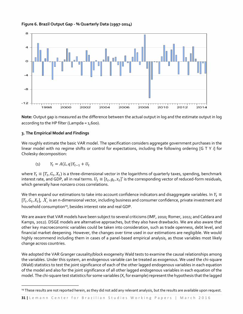
31 | L e m a n n C e n t e r f o r B r a z i l i a n S t u d i e s W o r k i n g P a p e r s | M a r c h 2 0 1 6
Figure 6. Brazil Output Gap - % Quarterly Data (1997-2014)
Note: Output gap is measured as the difference between the actual output in log and the estimate output in log
according to the HP filter (Lampda = 1,600).
3. The Empirical Model and Findings
We roughly estimate the basic VAR model. The specification considers aggregate government purchases in the linear model with no regime shifts or control for expectations, including the following ordering [G T Y i] for Cholesky decomposition:
(1) 𝑌𝑡 = 𝐴(𝐿, 𝑞)𝑌𝑡−1 + 𝑈𝑡
where 𝑌𝑡 ≡ [𝑇𝑡 , 𝐺𝑡 , 𝑋𝑡) is a three-dimensional vector in the logarithms of quarterly taxes, spending, benchmark interest rate, and GDP, all in real terms. 𝑈𝑡 ≡ [𝑡𝑡, 𝑔𝑡 , 𝑥𝑡]′ is the corresponding vector of reduced-form residuals, which generally have nonzero cross correlations.
We then expand our estimations to take into account confidence indicators and disaggregate variables. In 𝑌𝑡 ≡
[𝑇𝑡 , 𝐺𝑡 , 𝑋𝑡], is an n-dimensional vector, including business and consumer confidence, private investment and
household consumption19, besides interest rate and real GDP.
We are aware that VAR models have been subject to several criticisms (IMF, 2010; Romer, 2011; and Caldara and Kamps, 2012). DSGE models are alternative approaches, but they also have drawbacks. We are also aware that other key macroeconomic variables could be taken into consideration, such as trade openness, debt level, and financial market deepening. However, the changes over time used in our estimations are negligible. We would highly recommend including them in cases of a panel-based empirical analysis, as those variables most likely change across countries.
We adopted the VAR Granger causality/block exogeneity Wald tests to examine the causal relationships among the variables. Under this system, an endogenous variable can be treated as exogenous. We used the chi-square (Wald) statistics to test the joint significance of each of the other lagged endogenous variables in each equation of the model and also for the joint significance of all other lagged endogenous variables in each equation of the model. The chi-square test statistics for some variables (X, for example) represent the hypothesis that the lagged
19 These results are not reported herein, as they did not add any relevant analysis, but the results are available upon request.
Xt

32 | L e m a n n C e n t e r f o r B r a z i l i a n S t u d i e s W o r k i n g P a p e r s | M a r c h 2 0 1 6
coefficients of that variable in the regression equation of another variable (Y, for example) are equal to or different from zero. If equal to zero, that variable (X) is Granger causal for Y at some level of significance, which suggests that Y is not influenced by X. The null hypothesis of block exogeneity is then rejected for all equations in the model.
The first group of empirical results is related to a very simplified VAR model and its pairwise Granger causality and block exogeneity Wald tests. Information criteria from Akaike, Hannan-Quinn and Schwarz were used to select the most parsimonious, correct model. Most tables and figures presenting the results appear in the Annex. We have conveniently separated some figures to show alongside the text.
We estimated two different VAR models as follows:
(1) VAR 2: [Y, S, T, i]
where Y is the GDP; S is the government expenditure as a percentage of GDP deflated by IPCA; T is the net tax revenue as a percentage of GDP deflated by IPCA; and i is the Selic interest rate in annual percentage terms.
(2) VAR 1: [h, FI, i]
where h is the output gap measure, i.e., the difference between the actual GDP and the potential GDP according to the HP filter; FI is the fiscal impulse measure, i.e., the variation of the primary surpluses as a share of GDP; and i is the variation of Selic interest rate in annual percentage terms.
The VAR model in specification (2) allows us to simultaneously identify the direction of fiscal and monetary policy. As we split up the sample to cope with the 2008 crash, it is also possible to observe the eventual shift in the economic policy stance before and after the crisis.
Then, this second specification is more related to the policy stance, whether countercyclical or pro-cyclical. For instance, fiscal policy could be labeled as countercyclical or pro-cyclical when the sign of the fiscal impulse is equal to or different from (expansionary or contractionary, respectively) the signal of the deviation of the real output from its tendency level (the output gap). Figure 7 illustrates this idea. According to this figure, one can have, for example, countercyclical policy under fiscal adjustments and pro-cyclical stances during output expansion. It is always a matter of the direction of the fiscal policy alongside the business cycle.
Figure 7. Fiscal Expansion and Contraction
GDP Output
Fiscal
Impulse
Output Gap (-) Output Gap (+)
Expansion (-) Countercyclical Pro-cyclical
Contraction (+) Pro-cyclical Countercyclical
There have been many discussions about countercyclical versus pro-cyclical fiscal policies and when and how much to utilize each type. However, the first challenge involves assessing how much effort policymakers intend to make. The most accurate way to infer this effort is by assessing structural fiscal results instead of conventional

33 | L e m a n n C e n t e r f o r B r a z i l i a n S t u d i e s W o r k i n g P a p e r s | M a r c h 2 0 1 6
ones20. Before moving on, it is important to consider that the structural fiscal results are still behind the times when the topic is fiscal rules, mainly because they are well known only quarters or even years after the fiscal practice is implemented, as they depend on many complex calculations. However, if the purpose is to define the intensity of the fiscal policy, they are more appropriate, even though the other methods are not necessarily incorrect.
The structural fiscal results can be briefly defined as results that are consistent with the potential output, under the condition of equilibrium in the asset and commodity prices and free of one-off revenues. It may be considered an accurate form to express the fiscal discretionary effect on the aggregate demand. As fiscal results can be influenced by many factors beyond the control of economic authorities, structurally-based results consider only the effective fiscal efforts of policymakers. Conventional results, such as primary surpluses, are not capable of measuring such efforts because they depend on others factors, such as the business cycle, and, in turn, changes in asset and commodity prices, changes in output composition, and one-off revenues.
Figure 8 illustrates the use of one-off revenues in Brazil, which increased dramatically after the 2008 crisis. One-off revenues includes: concessions revenue in most years, judicial deposit (in 2009), Eletrobras’ dividend (in 2009 and 2010), Petrobras capitalization (most of 2010 one-off revenue), Sovereign Fund of Brazil (created in 2008 and used in 2012), tax refining program (in 2009, 2011, 2013, and 2014), other one-off revenues, dividends in advance, and FND subsidies. The annual average of one-off revenue from 2009 to 2014 (after the crisis) was 0.6% of GDP when the average of the annual primary surpluses was 1.8% of GDP, representing, then, 1/3 of the annual fiscal results. How much policymakers intend to pledge or cut in terms of stimulus or retrenchment, respectively, during a certain period of time, depends on the fiscal impulse, that is, the difference between the current structural fiscal result and the previous result. Fiscal policy could be labeled as countercyclical or pro-cyclical when the signal of the fiscal impulse is equal to or different from (expansionary or contractionary, respectively) the signal of the deviation of the real output from its tendency level (the output gap).
Figure 8: One-Off Revenue, 2002-2014 (US$ Billion and % of GDP)
Source: Secretariat of Economic Policy, Minister of Finance of Brazil.
Notes: We use 3.0 Brazilian Real per one US Dollar.
20 See Bornhorst et al. (2011) for numerous technical issues associated with this concept.
-4000,0
-2000,0
0,0
2000,0
4000,0
6000,0
8000,0
10000,0
12000,0
14000,0
2002 2003 2004 2005 2006 2007 2008 2009 2010 2011 2012 2013 2014
0,74
0,02 0,06 0,04 0,04 0,08
-0,23
0,740,85
0,38
0,53
0,68
0,50
-0,40
-0,20
0,00
0,20
0,40
0,60
0,80
1,00
2002 2003 2004 2005 2006 2007 2008 2009 2010 2011 2012 2013 2014
% GDP

34 | L e m a n n C e n t e r f o r B r a z i l i a n S t u d i e s W o r k i n g P a p e r s | M a r c h 2 0 1 6
Here, the idea is different for the case of monetary policy. It could be pro-cyclical or countercyclical when the signal of the monetary policy shock (changes in the interest rate) is equal to or different from (contractionary or expansionary, respectively) the output gap. Then, for instance, we label arbitrarily a pro-cyclical monetary policy when the interest rate increases during an expansion. Otherwise, it would be a countercyclical orientation.
We also conducted a multivariate pairwise Granger causality test/block exogeneity Wald test derived from the VAR model to examine additional causal relationships between the key variables in the model. This test estimates the χ square value of the coefficients of lagged endogenous variables. The null hypothesis in this test is that the lagged endogenous variables do not Granger cause the dependent variable.
Data Descriptions
The models are estimated over three samples: first, the full sample spanning from 1997 to 2014 and then two other samples to determine the eventual effect of the 2008 crash: one from 1997 to 2007 and one from 2008 to 2014. We are aware that the small size of the sample of times series diminishes the degrees of freedom and the robustness of the estimates.
Table 3 shows data descriptions and the sources used here. All series, if necessary, are deflated with the Broad Consumer Price Index (IPCA) and divided by GDP.
According to our sample, the GDP has grown an average of 0.73% in quarter-over-quarter terms, which is approximately 3.0% in annualized terms; investment has grown a little faster at 3.2%; and consumption is coupled with the GDP growth (table 4). There are different speeds over time because investment has grown faster and consumption has resumed faster than the GDP after the 2008 turmoil. The average investment as share of GDP is 18.7%, with some increases after the crisis coming to approximately 20%, which could introduce an intriguing question. Net tax revenue as share of GDP has been higher than the government spending-to-GDP ratio. The volatility of the investment rates- as measured by standard deviation (approximately 14% in annualized terms)- is quite remarkable.
Table 3. Data descriptions and sources
Variable Source
Real GDP IBGE
General Government Primary Surplus Ministry of Finance
Net Federal Tax Revenue (total government revenue minus net transfers)
Ministry of Finance
General Government Consumption Ministry of Finance
Business Confidence Indicator CNI, FGV, and Fecomercio
Household Confidence Indicator CNI, FGV, and Fecomercio
Private Investment (Fixed Capital Gross Formation) IBGE
Household Consumption IBGE
Broad Consumer Price Index (IPCA) IBGE
Benchmark Nominal Interest Rate (Selic) Central Bank of Brazil

35 | L e m a n n C e n t e r f o r B r a z i l i a n S t u d i e s W o r k i n g P a p e r s | M a r c h 2 0 1 6
Table 4. Basic Statistics for 1997-2014 (N=72, QoQ Change)
GDP Growth (%)
Investment Growth (%)
Consumption Growth (%)
Investment (%GDP)
Tax Revenue (%GDP)
Governement Spending (%GDP)
Minimum -4.09 -10.0 -3.0 18.4 13.4 13.7
Maximum 2.76 8.5 2.98 21.6 24.7 20.9
Mean 0.73 0.79 0,72 18.7 17.7 16.03
Standard Deviation
1.17 3.3 1,14 1.45 1.8 1.47
Empirical Findings
Our models were generally run with four lags, according to the information criteria21. We estimate a model for the full sample (1997-2014) and for the period before (1997-2007) and after (2008-2014) the crash22. We first present results of the impulse-response functions and then the VAR Granger causality tests/block exogeneity Wald tests, from the VAR 1 specification and then from the VAR 2 specification. The figures and tables presenting these results appear in the Annex.
First, generally speaking, it is remarkable that the fiscal stimulus via government spending has a positive and statistically significant impact on GDP growth and that the monetary policy has a negative and statistically significant impact on GDP growth, regardless of the model and specification. It is also worth mentioning the channels through which these findings work in the model. On the one hand, unexpected shocks in government expenditures generally spark growth; on the other hand, they lead to positive shocks in the short-term interest rate that hinder growth. Additionally, there is no statistically significant response from any other key macroeconomic variable, including GDP growth and the confidence related to unexpected shocks in net tax revenue. However, tax revenue responded slightly positively to shocks in government expenditures and growth. There are mixed results associated with the relationship among our other key variables, such as government expenditures, net tax revenues, the fiscal impulse and the short-term interest rate.
More specifically, we first examine the impact of the unexpected structural shock of taxes on other key variables. According to the VAR Granger causality/block exogeneity Wald test, we cannot reject the null hypothesis that net tax revenue does not Granger cause GDP growth, but we can reject the hypothesis that it does not cause government expenditures. GDP growth Granger causes tax revenue only when we use the full sample and with less statistical significance when we use the bub-samples from after/before the crash.
According to the impulse-response functions, the response of GDP growth to unexpected shocks in tax revenue is small and not statistically significant; the size of the response and its significance is reasonable only when we take the short-term interest rate out of the VAR specification. In line with the Granger causality test, the response of government spending to a tax shock is positive and statistically significant.
Therefore, we can summarize the role played by tax policy as follows: increased government spending increases tax revenue, and the greater the GDP growth, the greater the tax revenue. It seems that tax revenue has increased because the government has chosen to stimulate the economy using its spending power.
21 The following information criteria are used here: LR = sequential modified LR test statistic (each test at the 5% level); FPE = final prediction error, AIC = Akaike information criterion; SC = Schwarz information criterion; and HQ = Hannan-Quinn information criterion. 22 Many details of some results were intentionally shortened, mostly because of their lack of significance; they are available upon request.

36 | L e m a n n C e n t e r f o r B r a z i l i a n S t u d i e s W o r k i n g P a p e r s | M a r c h 2 0 1 6
Now, we turn to the effect of the structural shock of government expenditures. According to the Granger causality test, one can reject the hypothesis that government spending does not Granger cause GDP growth, regardless of the sample and the specification.
On the other hand, government spending Granger causes the benchmark interest rate. Therefore, fiscal policy seems to be very efficient in reviving growth in Brazil, even though it comes with tax increases and a higher short-term interest rate.
In terms of dynamic effects, the GDP growth responds positively, although not necessarily different from zero, to unexpected shocks in government expenditures, reaching its peak after four quarters; its peak changes with the sample; using the full sample, the peak is 0.5, but the peak doubles to 1.1 in the period after the 2008 crash; it is approximating 0.4 for the sample before the crash. It seems that fiscal policy is even more effective during difficult times. In sum, the size of such impact, which is generally associated with the fiscal multiplier, is approximately 0.5 after 4 quarters for normal times and approximately 1.1 after four quarters in difficult times, including the aftermath of the 2008 financial crisis23.
Meanwhile, GDP growth responds negatively and statistically significantly to the unexpected shock in the benchmark interest rate. Surprisingly, the response is close to 1.1 for the sample after the crisis and 0.5 for the full sample and the sample before the crisis. There is no difference between the monetary and fiscal shocks in terms of the dynamics over time because both affect the GDP after four quarters.
As the monetary shock had a negative effect on GDP growth and GDP growth responded positively to the fiscal shock, it seems that the economic policy “has given poise to growth with one hand and taken it with the other one”.
For instance, some authors have conducted studies on the impact of the rock-bottom interest rate policy in the US. According to a general New Keynesian model, as explored in Christiano, Eichenbaum and Rebelo (2010), the government spending fiscal multiplier can be larger than usual thanks to the monetary policy stance. They analyzed a special case of the zero-lower-bound interest rate policy in the US and concluded that this policy amplifies the impact of expansionary stimuli.
According to these authors, “First, when the central bank follows a Taylor rule, the value of the government-spending multiplier is generally less than one. Second, the multiplier is much larger if the nominal interest rate does not respond to the rise in government spending. For example, suppose that government spending goes up for 12 quarters and the nominal interest rate remains constant. In this case the impact multiplier is roughly 1.6 and has a peak value of about 2.3. Third, the value of the multiplier depends critically on how much government spending occurs in the period during which the nominal interest rate is constant…for government spending to be a powerful weapon in combating output losses associated with the zero-bound state” (p. 5-6).
Does the monetary policy amplify the fiscal policy in the Brazil case? The answer is “no”. The monetary policy rate has been diminishing over time but has been reacting to the fiscal policy. It is a sort of “give-and-take policy”, as the persistently high short-term interest rate (see figure 9) under a conventional Taylor rule-based action considerably reduces the government spending fiscal multiplier. We also use the actual US federal funds rate to run a VAR that hypothetically assumes a zero-lower-bound monetary policy in Brazil. In such a hypothetical situation, the response of GDP growth to unexpected shocks in government expenditures would almost double, from 0.5 to 1.0 using the full sample and from 1.1 to 1.8 using sample after the 2008 crash, both under the dramatic assumption of a zero-lower-bound interest rate in Brazil. Figure 9 shows this story. For instance, the
23 We, herein, are intentionally not using such coefficients as the well-known fiscal multiplier because of drawbacks in the econometric analysis conducted in this research.

37 | L e m a n n C e n t e r f o r B r a z i l i a n S t u d i e s W o r k i n g P a p e r s | M a r c h 2 0 1 6
short-term interest rate increased from 2009 to 2012, and, after a lax cycle, another tight policy stance arose in 2013. While fiscal policy was predominantly operating in a countercyclical direction, monetary policy was operating in a pro-cyclical direction.
Figure 9: Benchmark Nominal Interest Rate (2008-2015), annual %
Source: Central Bank of Brazil
Now, we use the VAR 2 [h, F, i] specification to analyze the direction, i.e., countercyclical or pro-cyclical, of economic policy. The VAR was run with four lags following the information criteria. At first glance, as seen in figure 11, fiscal policy has been predominantly countercyclical, and monetary policy has been predominantly pro-cyclical24. An unexpected shock in the fiscal impulse (the change in the primary surplus-to-GDP ratio) has a positive and statistically significant impact on the output gap (the difference between the actual GDP and its potential level). One can clearly see that the government increases its fiscal results when the economy is doing better and reduces them under contractions. According to the impulse-response function, the fiscal impulse responds positively and statistically significantly to the unexpected shock of GDP growth, and vice versa, reaching a peak of 1.2 after three quarters and remaining relatively stable afterwards. Using the sub-sample after the 2008 crash, this peak jumps up to 1.9, which clearly shows the important role played by fiscal stimuli during hard times.
24 Again, we arbitrarily labeled “pro-cyclical” monetary policy when the interest rate follows the business cycle in the same direction. This case could fairly be denominated as a counter-cyclical fiscal policy.
11.25
7.25
14.25
4
6
8
10
12
14
16
1/1
/2008
4/1
/2008
7/1
/2008
10/1
/2008
1/1
/2009
4/1
/2009
7/1
/2009
10/1
/2009
1/1
/2010
4/1
/2010
7/1
/2010
10/1
/2010
1/1
/2011
4/1
/2011
7/1
/2011
10/1
/2011
1/1
/2012
4/1
/2012
7/1
/2012
10/1
/2012
1/1
/2013
4/1
/2013
7/1
/2013
10/1
/2013
1/1
/2014
4/1
/2014
7/1
/2014
10/1
/2014
1/1
/2015
4/1
/2015
7/1
/2015
10/1
/2015

38 | L e m a n n C e n t e r f o r B r a z i l i a n S t u d i e s W o r k i n g P a p e r s | M a r c h 2 0 1 6
Figure 10. Impulse-Response Function VAR [Y, S, T, i]
Meanwhile, unexpected shocks in monetary policy have a negative and statistically significant impact on the output gap. Monetary policy in Brazil seems more effective than expected. In a dynamic analysis, the output gap slump in response to the unexpected monetary shock, bottoming out at -0.5 after two quarters, then increases to -1.7 after five quarter, remaining relatively stable afterwards. During tough times, using the sub-sample from 2008 to 2014, this peak elevates to 2.0. The main lesson that we can take from these empirical findings is that monetary shocks have been large enough to counterweigh any fiscal stimulus over time.

39 | L e m a n n C e n t e r f o r B r a z i l i a n S t u d i e s W o r k i n g P a p e r s | M a r c h 2 0 1 6
It is worth mentioning that monetary policy has reacted to fiscal policy because the benchmark interest rate responds negatively to unexpected shocks in the primary surplus. We were not able to accept the responses of the interest rate set by the Central Bank to shocks nor to net tax revenue nor to government spending, but we can now observe the importance of primary surpluses to the Central Bank of Brazil’s decision-making process. According to our VAR specification, a 100 basis-point increase in the primary surplus as share of GDP triggers a 30 basis-point decreases in the short-term interest rate after two quarters.
Figure 11. Impulse-Response Function VAR [h, F, i]
We also include indicators of confidence in variations of both of our VAR specifications25. As there would be a causal relationship running from the indicators of business and consumer confidences to output and investment, we inquired about whether confidence might be resumed before investment and output. According to Alesina et al. (2014), “the confidence of investors also does not decrease much after an expenditure-based adjustment and promptly recovers and increases above the baseline; it instead falls for several years after a tax-based adjustment”.
25 These empirical results are not reported here for convenience, as they did not add any relevant information to our analysis; they are available upon request.

40 | L e m a n n C e n t e r f o r B r a z i l i a n S t u d i e s W o r k i n g P a p e r s | M a r c h 2 0 1 6
As leading indicators, indicators of business and consumer confidences could be able to foresee prospects of output and investment for the coming years. However, the results when we run specifications that include such variables do not change our previous findings. Confidence indicators, both for businesses and consumers, respond less than GDP growth to shocks in government expenditures, net tax revenues, and fiscal impulses. It seems that when the scenario for growth comes to entrepreneurs’ and consumers’ minds, the economy has already found a path to growth.
2014-2015 fiscal plan: impact and lessons
We now elucidate the program proposed by the Brazilian authorities to invigorate the fiscal front. Broadly speaking, two groups of measures have been already announced. The first set of measures was announced in December 2014 and focused on reviewing some social benefits. At that time, the intention to both reduce the financial subsides of the BNDES (National Bank for Social and Economic Development) funding and, as prescheduled, increase taxes for industrialized goods, mainly in the automobile sector, was announced. In late January 2015, a general increase in tax rates, including on domestic credit was announced. Tables 5.1 and 5.2 summarize these measures and their expected fiscal impacts. A tax hike is a sort of one-off shock, and a spending cut might produce increased savings over time, mainly because of changes in social benefits. Since then, other measures were put forward related to both expenditure cuts and tax increases.
According to the table 5.1 and 5.2, in the best-case scenario, a positive fiscal impact of 2.2% of GDP was estimated for 2015, when spending cuts would respond to most of the fiscal retrenchment. Despite the political risks of its approval, it could be considered a promising beginning for a fiscal program. Such fiscal efforts would theoretically be sufficient to move from a primary deficit of 0.6% of GDP in 2014 to the target surplus of 1.2% of GDP in 2015. However, tax revenue also responds to GDP growth with elasticity greater than a unity. A prospect of 3.5% of GDP contraction cannot easily offset the expected increase in tax revenue associated with the recent tax hikes. Additionally, a partial congressional approval of the fiscal package lowers expectations for a reasonable 2015 fiscal result.
We now use our empirical findings to estimate the impacts of such fiscal announcements on output and confidence. The size of fiscal retrenchment could be theoretically considered around 2.2% of GDP— 0.54% of GDP in tax hikes and 1.75% of GDP in spending cuts. Yet, it is an overestimated fiscal shock, since only 0.26% of GDP is associated to cuts in structural government spending. Then, from 0.8% to 1.0% of GDP would be a more accurate size of the fiscal shock due to 2015.
What can these empirical results tell us about the recently announced fiscal measures? According to our estimates, a 1% of GDP change in government spending contributes to 0.5 p.p. of the GDP change after four quarters in normal times, and it can contribute up to 1.1 p.p. of the GDP change in difficult times. In this case, the 2015 proposal of fiscal retrenchment is likely to respond to roughly one quarter of the contraction in 2015. We are aware that this metric is not a terribly accurate measurement of the recent fiscal retrenchment—not because of our own skepticism with such empirical evidence, as we were not able to run a broad model, but because there is no an accurate timeline associated with the calendar year for econometrics. Additionally, potential output may change more quickly than expected.
As we learned from our exercises, the pro-cyclical stance of the monetary policy dramatically increases the impact of the fiscal consolidation on output. It is important to show that the monetary policy shock can be accounted for as an approximately 700 basis-point increase over a bit more of two-year interval, from April 2013 to July 2015. In addition, around half of the 2015 contraction and approximately one-quarter of the growth below its potential level in 2016 could be explained by a combination of both contractionary fiscal policy and monetary policy.
An avenue of literature supports that the claim that the beneficiary effect of fiscal expansionary measures in difficult times has been underestimated, the stance of the business cycle and whether the fiscal policy if pro-

41 | L e m a n n C e n t e r f o r B r a z i l i a n S t u d i e s W o r k i n g P a p e r s | M a r c h 2 0 1 6
cyclical or countercyclical have not been considered. According to Riera-Crichton et al. (2014), in difficult times, the spending multiplier is about 2.30 when there is a spending increase.
The harmful effects of austerity in difficult times have also been underestimated because the policy instrument (tax rates) has not been used. Instead, policy outcome measures based on tax revenue, such as cyclically adjusted measures, have been relied upon, as in the following equation: ,
where is the tax base to GDP elasticity. When using cyclically adjusted revenues, the result is not very
contractionary and can be neutral or even expansionary; however, when using tax rates, the result is very contractionary (Riera-Crichton, Vegh and Vulletin, 2014).
The Brazilian economy has only recently graduated to respond to the crisis using fiscal policy (Végh and Vulletin, 2013). Until the 2008 financial crisis, Brazil was unable to introduce expansionary policy when the output gap was negative. The 2008 crisis proved that Brazilian solvency was no longer a major issue, and a comprehensive set of measures could help the country to stymie the contamination of the worsening scenario experienced abroad and to resume growth more quickly. The country context has already been discussed in a previous section.
We can learn two lessons here. First, there is a narrower-than-expected borderline to use both orientations (either counter or pro-cyclical) imposed by either debt dynamics, in case of countercyclical fiscal policy, or the real output and unemployment levels, otherwise. Second, despite the orientation, there is not an easy way to obtain sound fiscal results swimming against the current. In line with what was expected for countercyclical fiscal policy, as figure 6 showed the economy running well below its potential, most of the 2013-2014 period was dedicated to a negative fiscal impulse (expansion) when the output was predominantly negative (contraction). Along with frustrated growth26, the fiscal situation was getting worse. Solvency issues were again a problem. Hence, a pro-cyclical fiscal policy was implemented at the end of 2014 in an effort to cope with sovereign ratings.
26 The plausible reasons why the Brazilian economy was not able to resume growth even with fiscal stimulus are out the scope of this work. However, we hardly find theoretical or empirical support for any association between the recent weakness and only one factor.
h

Table 5.1. Fiscal Measures*: Spending Cuts US$ Billion**
Description Current Spending
(2014)
Estimated Spending (2015)
Fiscal Impact (US$)
2015 2016 2017 2018
1. Wage Bonus Establish criterion of proportionality according to the work time.
5,0
6,0 0,4 0,8 1,3 1,4
2. Unemployment Insurance
Increase the grace period to 12 months for the first request and to 9 months for the second request, instead of 6 months.
11,0
12,7 1.6 2,8 3,2 3,8
3.Illnesss Aid*** Increase coverage time in charge of the private sector to 30 days, instead of 15 days and change the calculation of the benefit.
6,7 8,0 0.4 2,5 3,0 4,0
4.Widow/Widower Pension
Establish criteria to be eligible as 24 months of contributions, at least 2 years of marriage, end of lifetime benefit, criterion of proportionality associate with the age of the beneficiary, and reduction in case of dependents.
30,0 33,0 0,8 2,0 2,8 3,7
5. 2015 Federal Budget
Budget cut 23.3****
20,0****
20,0****
20,0****
Total of Expenditure Cuts
26.5 28,0 30,3 32,9
% of GDP **** 1.40 1.44 1,56 1,69
Notes: *As approved by the Congress in May 7th, 2015; **3.0 Real per Dollar; *** This measure was not approved. **** 2015 according to the new 2015 Annual Budget Law announced last May 22th; otherwise, are suggested annual budget cut according to the recent experience only to illustrate the overall impact in upcoming years; ****Nominal GDP for 2015 is estimated as US$1,886 million (Bacen, June 2015), and 10% nominal annual increases for other years.

Table 5.2. Fiscal Measures: Tax Increases US$ Billion*
Description Fiscal Impact 2015 (US$)
1. Financial Transaction Tax Increase in the tax rate to 3,0% from 1,5% for consumption credit transactions
2,50
2. Fuel tax Increase in the PIS/Cofins rate on fuel and in Cide-Gasoline to R$0,22/liter and also in Cide-Oil to R$0,15/liter
4,00
3. Payroll Tax Increase in the rates from 1,0% and 2,0% to 2,5% and 4,5%, respectively, to targeted sectors
0.9***
4. Automotive Tax Return to normal rates in the Industrialized Product Tax to the automobile sector
1,0
5. Export Tax benefit Reduction in the tax rebate to the export sector to 1% from 3% of the export revenue.
0,60
6. Import Tax Recovery of PIS/Cofins rate on import goods, after Supreme Court decision on ICMS, with new rate of 11,75%.
0,23
7. Cosmetic Tax Rate isonomy between wholesale and industry 0,13
8. Beverage Tax New tax regime for the beverage sector 0,50
9. Income Tax Presidential veto to 6,5% linear correction on the 2015 income tax table
1,00
10. Financial institution Increase in the rate of CSLL from 15% to 20% 0.25
11. Financial returns Rate of 4.65% in PIS/Cofins on financial returns 0.90
Total of Tax Increases (US$)
12.0
% of GDP** (%) 0,64
Notes: * 3.0 Real per Dollar; ** Nominal GDP for 2015 is estimated at US$1,866 million (Bacen, June 2015), and 10% nominal annual increases for other years. *** This measure is still under discussion.
Many other measures were announced along 2015 (see table 5.3) and are pending in Congress to be approved. More expenditures were cut, mainly those related to investment, and some tax exemptions were withdrawn as the case of payroll tax benefits. An ambiguous discussion inside the government has put doubt on its economic policy stance. Some authorities support the idea of coming back with stimuli to resume growth; other ones emphasize the route of austerity as the only way to recovery confidence. Uncertainty has been amplified and the economy is falling into an abyss. Nine months after the fiscal adjustment plan had been announced, by September 2015, net tax revenue dropped 4.6%, in a year-to-date term, and meanwhile the primary expenditures dropped 4.0%. These results have not been enough to reach a reasonable fiscal balance. A fiscal crisis was installed.

44 | L e m a n n C e n t e r f o r B r a z i l i a n S t u d i e s W o r k i n g P a p e r s | M a r c h 2 0 1 6
Table 5.3. Measures Pending in Congress – announced along 2015
Description Fiscal Impact in 2016 (US$ billion*)
1. DRU (non-earmarking of revenue)
Postpone the execution of the DRU until December 2019
40
2. CPMF Re-create the CPMF tax with a 0.2% rate to be in place until December 2019.
10
3. Repatriation Allows of the repatriation of undeclared resources 2.0
4. Electronic subsidy Removal of electronic subsides with higher PIS/Cofins tax on computer, phones and tables.
2,3
5. Prorelit The program which allows companies to use fiscal loss and CSLL credits to honor legal dispute losses with the government.
3,3
6. Capital Gain Capital gain tax today is a fixed 15% rate. The measure crates progressive brackets on the capital gains taxes.
0,6
7. IOC (interest on own capital)
Limits the IOC benefit for companies to the TJLP or 5%, whichever is lower.
0,6
Total (US$ billion) 58.8
Notes: *3.0 Real per Dollar.
Lessons learned
We now move on to propose a fiscal framework from the lessons that we have recently learned. Regardless of short-term concerns, a consistent fiscal plan emerged from international experiences and from our simplified empirical exercise; this plan should have key components. We summarize them below.
First, the fiscal announcement has to be a “plan” rather than a “shock”. Here, we benefit from the research conducted by Alesina et al. (2014). In their empirical findings, a multi-year spending-based fiscal plan is much less costly than a tax-based fiscal shock. According to the authors, “The difference between tax-based and spending-based adjustments appears not to be explained by accompanying policies, including monetary policy. It is mainly due to the different responses of business confidence and private investment”.
Although designed with medium-term intentions, fiscal programs have been announced in Brazil as fiscal shocks rather than as a medium- to long-term plan. Fiscal announcements have to be perceived longer than the previous ones, such as the 2011 fiscal consolidation, and they have to be communicated with clear commitments. In this case, the overall annual fiscal target, such as a primary surplus, should be taken as a means rather than an end. Therefore, monetary policy would adapt to reach its central inflation target and to maintain it for long period of time. Inflationary risks would also dissipate, taming inflation expectations to the central targets.
Fiscal policy must leave clear room for a more accommodating monetary policy, only after the fiscal policy has been observed as an anchor with de facto recurrent fiscal results. Tax relief for investment and production, mainly through broad tax reform, will be welcomed as possible. Such a well-designed fiscal plan that is clearly communicated and regularly double-checked with recurrent accountability and transparency might hurt short-term economic growth, although the country will then be able to move toward consistent growth rates.
The main corollary of such a fiscal plan would be a complete change in the incentives for investing and saving. The plan has to last for a sufficiently long period, and it has to be deep and wide to reach such achievement.

45 | L e m a n n C e n t e r f o r B r a z i l i a n S t u d i e s W o r k i n g P a p e r s | M a r c h 2 0 1 6
Therefore, both short- and long-term interest rates gradually decrease, thus promoting funding for long-term investment. Concurrently, the “short-termism mania” is being addressed because persistently high inflation rates lead to high short-term real interest rates and fewer stimuli in the process of lengthening assets and liabilities.
Second, a new institutional framework should be developed, including an independent fiscal council and multi-year targets for gross debt-to-GDP ratios with debt ceiling27. A band of tolerances would be welcome, which makes this policy politically more feasible and also leaves room for countercyclical actions during difficult times. The general government debt is what an emerging market economy, such as Brazil, needs to deliver an idea of intertemporal solvency, especially when the country has a history of defaults and low debt thresholds according to the debt intolerance literature (Reinhart et al., 2003). Consequently, the lower the solvency risk, the lower the short-term interest rate. Persistently low inflation rates and government debts are the conditions for sustainable low short-term real interest rates (Bacha, Holland, and Gonçalves, 2007 and 2009).
Only conventional monetary policy anchored in a long-standing fiscal policy framework will allow Brazil to progress to the next stage in macroeconomic fundamentals and, therefore, in long-term investors’ perceptions.
Third, the fiscal plan has to be based on spending cuts rather than on tax hikes (Alesina et al., 2014). We warn that all these economic measures should be taken as only the beginning of a plan28. An overall revision of government expenditures has to be implemented, including an overwhelming reform agenda for the entire pension system and for several other social benefits, including the education system29. Meanwhile, comprehensive tax reform should reduce both the tax system’s complexity and its management costs, which have provoked high judicial uncertainty. Under the current macroeconomic circumstances and prospects, tax reform has to be fiscally neutral.
Fourth, the fiscal plan tailored for the Brazilian case has to go beyond fiscal efforts and challenge itself to improve the relationship between the state and the private sector. Most state-owned companies should enter into the market to seek private strategic alliances. On the one hand, this move would make public accounting more transparent, and, on the other hand, it would benefit fiscal results. However, the main purpose of such policy recommendations is to rebalance the broad spectrum of the state’s involvement in the economy.
Finally, as widely recommended by many analysts, we would add a rule for government spending dynamics over time. As some expenditures have mandatory limits, it would be recommendable emphasize this new rule of government spending ceiling as a superior legal rule over the specific ones, such as those social and pension benefits, for education, and health.The long-term fiscal plan for the Brazil would seek to ensure that expenditure growth does not exceed the nominal GDP growth. This rule could be added through an amendment to the existing Law of Fiscal Responsibility, in which the independent fiscal council and the long-term government gross debt targets should be included.
It is also worth considering limits in the subsided credits, except those for the agricultural sector. The generation of finance subsides to be paid years ahead put constraints to upcoming fiscal results. Low interest rates without subsidy would be enough to stimulate the economy during tough periods. Again, only the National Congress
27 The current target to primary surplus is the only means to reach debt ratios. Another target would be the structural fiscal result which is known only after some time ahead, despite its complexity and sensibility to unobserved variable as the potential output. For the initiative of the Senator Jose Serra, the Congress has discussed to limit gross debt to RCL (net current revenue), that is, the tax revenue minus mandatory constitutional transfers. If approved, it would be a great advance. 28 We offer this warning despite the fact that the author of this paper was fully involved in designing the set of measures announced late 2014 and early 2015. 29 Another model for financing higher education would be welcome.

46 | L e m a n n C e n t e r f o r B r a z i l i a n S t u d i e s W o r k i n g P a p e r s | M a r c h 2 0 1 6
would be able to authorize financial subsidy under extreme circumstances, as well as allow the Government to exceed the debt ceiling.
Linked to the latest recommendation, it must require a comprehensive assessment on the fiscal impact of every public policy for its lifetime rather than either a cash-flow or a short-term assessment. The new independent fiscal council would be empowered to supervise such analysis and issue its formal statement. Only after such procedure, the government would be authorized to implement the policy. It has to have no impact in the gross debt to GDP ratio over time and respect the spending rule at the same time. Extreme situations such as natural disasters and war would be considered exceptions.
It is important to reiterate that there is no simple and widespread fiscal rule that suits all countries well, as there is, for example, for Central Bankers. Tailored fiscal rules according to the each country’s circumstances, even though they may seem discretionary at first glance, could also be more effective in reaching, sustaining, or even enhancing a country’s credibility and reputation. Moreover, a tailored fiscal rule can hardly be expressed in a single equation or with even with an algorithm. Because of this complexity, DGSE models will most likely underestimate the dynamic effects of fiscal policy on the output.
Final remarks
Fiscal policy was one of the most disputed issues after the 2008 crash. On the one hand, policymakers have still been trying to resume growth and to avoid the escalation of unemployment. On the other hand, the benchmark interest rates across the major advanced economies dropped towards zero-lower-bound, and they have remained there longer than anyone expected or desired. Meanwhile, fiscal policy stances have oscillated between expansion and austerity with fragile assessments of their effectiveness. Empirical findings are mixed and generally relate to the size of the government spending fiscal multiplier. It can range from a negative value to four!
We conducted empirical research to identify the impact of unexpected fiscal shocks on output. We estimated variations of VAR specifications to identify the dynamic effects and causality/endogeneity among our key macroeconomic variables. We also changed the sample to determine whether the 2008 crisis affected in the effectiveness of fiscal policy in some way. As Brazil is an extraordinary case of a country that persistently has one of the highest interest rates worldwide, we assessed the way that monetary policy works alongside fiscal stimuli.
As the title of this working paper suggests, we have good and bad news. The good news is that fiscal and monetary policies seem more effective than expected in Brazil. A government spending fiscal multiplier ranges between 0.5 and 1.1 after four quarters, for normal times and bad times, respectively. The bad news is that monetary and fiscal policies have moved in different directions because the fiscal policy is predominantly countercyclical and monetary policy is predominantly pro-cyclical in the way we defined. There is no guilty party and no innocent party. The monetary policy is only reacting to the effectiveness of the fiscal policy.
Moreover, we challenged ourselves to describe the channels in Brazilian economic policy. The higher the government spending, the higher the growth; meanwhile, the higher the tax revenues, the higher the Central Bank’s interest rate target. Growth losses are a corollary of monetary policy. We label it as a “give-and-take economic policy”.
One way to avoid from this trap, among many other recommendations, is to permanently decrease government expenditures to open the floor for tax relief and lower short-term interest rates in a well-designed long-term fiscal plan.

47 | L e m a n n C e n t e r f o r B r a z i l i a n S t u d i e s W o r k i n g P a p e r s | M a r c h 2 0 1 6
References Cited
ALESINA, A. and ARDGNA, S. 2009. Large chances in fiscal policy: taxes versus spending. NBER Working Paper #15438, October 2009.
ALESINA, A., FAVERO, C. and GIAVAZZI, F. 2014. The output effect of fiscal consolidation plan. (mimeo). AUERBACH, A. and GORODNICHENKO, Y. 2013. Fiscal multipliers in recession and expansion. A. ALESINA and F.
GIAVAZZI. 2013. Fiscal policy after the financial crises. NBER/Chicago Press. AUERBACH, A. and GORODNICHENKO, Y. 2011. Measuring the output response to fiscal policy. University of
California, Berkeley, June 2011. BACHA, E. M. HOLLAND, and F. GONÇALVES, 2009. Systemic Risk, Dollarization, and Interest Rates in
Emerging Markets: A Panel-Based Approach. The World Bank Economic Review, Vol. 23, Issue 1, pp. 101-117, 2009.
BACHA, E. M. HOLLAND, and F. GONÇALVES, 2007. Is Brazil Different? Risk, Dollarization, and Interest Rates in Emerging Markets. IMF Working Paper #07/294. December 2007.
BACHMANN, R. and SIMS, E. 2011. Confidence and the transmission of government spending shocks. NBER Working Paper #17063, May 2011.
CALDARA, D. and CHRISTOPHE KAMPS. 2012. The analytics of SVARs: a unified framework to measure fiscal multipliers. Finance and Economics Discussion Series 2012-20. Board of the Federal Reserve System, Washington, DC.
CHRISTIANO, L. M. EICHENBAUM, and S. REBELO. 2010. When is the government spending multiplier larger? Northwestern University, mimeo. December 2010.
EICHENGREEN, B. 2015. Hall of Mirrors: the great depression, the great recession, and the uses –and misuses- of history. Oxford University Press.
ESTAVAO, M. and SAMAKE, I. 2013. The Economic Effects of Fiscal Consolidation with Debt Feedback. IMF Working Paper May 2013.
GHOSH, A., and L. RAHMAN, 2008, “The Impact of Fiscal Adjustment on Economic Activity” (Washington: International Monetary Fund, unpublished).
BORNHORST, F. et al. 2011. When and How to Adjust Beyond the Business Cycle? A Guide to Structural Fiscal Balances. IMF Technical Notes and Manual. April 2011.
INTERNATIONAL MONETARY FUND. 2010. Will it hurt? Macroeconomic effect of fiscal consolidation. World Economic Outlook (October). Washington, DC: IMF, chapter 3.
ILZETZKI, E., 2011. Fiscal Policy and Debt Dynamics in Developing Countries. Policy Research Working Paper Series 5666 (Washington: The World Bank).
ILZETZKI E. et al., 2013. How Big (Small?) Are Fiscal Multipliers? Journal of Monetary Economics, Vol. 60, pp. 239–54.
KRAAY, A., 2012. How large is the Government Spending Multiplier? Evidence from World Bank Lending. Quarterly Journal of Economics, Vol. 127, No. 2, pp. 829–87.
MINESHIMA, A. et al. 2014. Size of Fiscal Multiplier. C. Cottarelli, P. Gerson, and A. Senhaji. 2014. Post-Crisis Fiscal Policy. MIT Press.
REINHART, C. et al. 2003. Debt intolerance. NBER Working Paper # 9908, August 2003. RIERA-CRICHTON, D et al., G. 2014. Procyclical and countercyclical fiscal multipliers: evidence from OECD
countries. NBER Working Paper #20533, September 2014. ROMER, C. 2011. What do we know about the effect of fiscal policy? Separating evidence from ideology. Speech
note at Hamilton College, Clinton, NY. VÈGH, C. A. And G. VULETIN. 2013. The Road to Redemption: Policy Response to Crises in Latin America. IMF
14th Jacques Polak Annual Research Conference. IMF, Washington, DC. November 2013.

48 | L e m a n n C e n t e r f o r B r a z i l i a n S t u d i e s W o r k i n g P a p e r s | M a r c h 2 0 1 6
ANNEX
VAR 1: [Y, S, T, i] Full Sample (1997-2014)
-2
-1
0
1
2
1 2 3 4 5 6 7 8 9 10
Accumulated Response of GDPGROWTH to GDPGROWTH
-2
-1
0
1
2
1 2 3 4 5 6 7 8 9 10
Accumulated Response of GDPGROWTH to DIFEXPEND04
-2
-1
0
1
2
1 2 3 4 5 6 7 8 9 10
Accumulated Response of GDPGROWTH to DIFTAX02
-2
-1
0
1
2
1 2 3 4 5 6 7 8 9 10
Accumulated Response of GDPGROWTH to DIFSELIC
-.02
.00
.02
.04
.06
1 2 3 4 5 6 7 8 9 10
Accumulated Response of DIFEXPEND04 to GDPGROWTH
-.02
.00
.02
.04
.06
1 2 3 4 5 6 7 8 9 10
Accumulated Response of DIFEXPEND04 to DIFEXPEND04
-.02
.00
.02
.04
.06
1 2 3 4 5 6 7 8 9 10
Accumulated Response of DIFEXPEND04 to DIFTAX02
-.02
.00
.02
.04
.06
1 2 3 4 5 6 7 8 9 10
Accumulated Response of DIFEXPEND04 to DIFSELIC
-.04
-.02
.00
.02
.04
.06
.08
1 2 3 4 5 6 7 8 9 10
Accumulated Response of DIFTAX02 to GDPGROWTH
-.04
-.02
.00
.02
.04
.06
.08
1 2 3 4 5 6 7 8 9 10
Accumulated Response of DIFTAX02 to DIFEXPEND04
-.04
-.02
.00
.02
.04
.06
.08
1 2 3 4 5 6 7 8 9 10
Accumulated Response of DIFTAX02 to DIFTAX02
-.04
-.02
.00
.02
.04
.06
.08
1 2 3 4 5 6 7 8 9 10
Accumulated Response of DIFTAX02 to DIFSELIC
-.2
.0
.2
.4
.6
1 2 3 4 5 6 7 8 9 10
Accumulated Response of DIFSELIC to GDPGROWTH
-.2
.0
.2
.4
.6
1 2 3 4 5 6 7 8 9 10
Accumulated Response of DIFSELIC to DIFEXPEND04
-.2
.0
.2
.4
.6
1 2 3 4 5 6 7 8 9 10
Accumulated Response of DIFSELIC to DIFTAX02
-.2
.0
.2
.4
.6
1 2 3 4 5 6 7 8 9 10
Accumulated Response of DIFSELIC to DIFSELIC
Accumulated Response to Cholesky One S.D. Innovations ± 2 S.E.

49 | L e m a n n C e n t e r f o r B r a z i l i a n S t u d i e s W o r k i n g P a p e r s | M a r c h 2 0 1 6
VAR 1: [Y, S, T, i] After 2008 Crisis (2008-2014)
-4
-2
0
2
4
1 2 3 4 5 6 7 8 9 10
Accumulated Response of GDPGROWTH to GDPGROWTH
-4
-2
0
2
4
1 2 3 4 5 6 7 8 9 10
Accumulated Response of GDPGROWTH to DIFEXPEND04
-4
-2
0
2
4
1 2 3 4 5 6 7 8 9 10
Accumulated Response of GDPGROWTH to DIFTAX02
-4
-2
0
2
4
1 2 3 4 5 6 7 8 9 10
Accumulated Response of GDPGROWTH to DIFSELIC
-.08
-.04
.00
.04
.08
1 2 3 4 5 6 7 8 9 10
Accumulated Response of DIFEXPEND04 to GDPGROWTH
-.08
-.04
.00
.04
.08
1 2 3 4 5 6 7 8 9 10
Accumulated Response of DIFEXPEND04 to DIFEXPEND04
-.08
-.04
.00
.04
.08
1 2 3 4 5 6 7 8 9 10
Accumulated Response of DIFEXPEND04 to DIFTAX02
-.08
-.04
.00
.04
.08
1 2 3 4 5 6 7 8 9 10
Accumulated Response of DIFEXPEND04 to DIFSELIC
-.10
-.05
.00
.05
.10
.15
1 2 3 4 5 6 7 8 9 10
Accumulated Response of DIFTAX02 to GDPGROWTH
-.10
-.05
.00
.05
.10
.15
1 2 3 4 5 6 7 8 9 10
Accumulated Response of DIFTAX02 to DIFEXPEND04
-.10
-.05
.00
.05
.10
.15
1 2 3 4 5 6 7 8 9 10
Accumulated Response of DIFTAX02 to DIFTAX02
-.10
-.05
.00
.05
.10
.15
1 2 3 4 5 6 7 8 9 10
Accumulated Response of DIFTAX02 to DIFSELIC
-0.5
0.0
0.5
1.0
1 2 3 4 5 6 7 8 9 10
Accumulated Response of DIFSELIC to GDPGROWTH
-0.5
0.0
0.5
1.0
1 2 3 4 5 6 7 8 9 10
Accumulated Response of DIFSELIC to DIFEXPEND04
-0.5
0.0
0.5
1.0
1 2 3 4 5 6 7 8 9 10
Accumulated Response of DIFSELIC to DIFTAX02
-0.5
0.0
0.5
1.0
1 2 3 4 5 6 7 8 9 10
Accumulated Response of DIFSELIC to DIFSELIC
Accumulated Response to Cholesky One S.D. Innovations ± 2 S.E.

50 | L e m a n n C e n t e r f o r B r a z i l i a n S t u d i e s W o r k i n g P a p e r s | M a r c h 2 0 1 6
VAR 2: [h, FI, i] Full Sample (1997-2014)
-4
-2
0
2
4
6
8
1 2 3 4 5 6 7 8 9 10
Accumulated Response of H to H
-4
-2
0
2
4
6
8
1 2 3 4 5 6 7 8 9 10
Accumulated Response of H to FISCALIMPULSE
-4
-2
0
2
4
6
8
1 2 3 4 5 6 7 8 9 10
Accumulated Response of H to DIFSELIC
-0.5
0.0
0.5
1.0
1.5
1 2 3 4 5 6 7 8 9 10
Accumulated Response of FISCALIMPULSE to H
-0.5
0.0
0.5
1.0
1.5
1 2 3 4 5 6 7 8 9 10
Accumulated Response of FISCALIMPULSE to FISCALIMPULSE
-0.5
0.0
0.5
1.0
1.5
1 2 3 4 5 6 7 8 9 10
Accumulated Response of FISCALIMPULSE to DIFSELIC
-.4
-.2
.0
.2
.4
.6
1 2 3 4 5 6 7 8 9 10
Accumulated Response of DIFSELIC to H
-.4
-.2
.0
.2
.4
.6
1 2 3 4 5 6 7 8 9 10
Accumulated Response of DIFSELIC to FISCALIMPULSE
-.4
-.2
.0
.2
.4
.6
1 2 3 4 5 6 7 8 9 10
Accumulated Response of DIFSELIC to DIFSELIC
Accumulated Response to Cholesky One S.D. Innovations ± 2 S.E.

51 | L e m a n n C e n t e r f o r B r a z i l i a n S t u d i e s W o r k i n g P a p e r s | M a r c h 2 0 1 6
VAR 2: [h, FI, i] after 2008 Crisis (1997-2014)
-10
-5
0
5
10
15
1 2 3 4 5 6 7 8 9 10
Accumulated Response of H to H
-10
-5
0
5
10
15
1 2 3 4 5 6 7 8 9 10
Accumulated Response of H to FISCALIMPULSE
-10
-5
0
5
10
15
1 2 3 4 5 6 7 8 9 10
Accumulated Response of H to DIFSELIC
-2
-1
0
1
2
1 2 3 4 5 6 7 8 9 10
Accumulated Response of FISCALIMPULSE to H
-2
-1
0
1
2
1 2 3 4 5 6 7 8 9 10
Accumulated Response of FISCALIMPULSE to FISCALIMPULSE
-2
-1
0
1
2
1 2 3 4 5 6 7 8 9 10
Accumulated Response of FISCALIMPULSE to DIFSELIC
-.8
-.4
.0
.4
.8
1 2 3 4 5 6 7 8 9 10
Accumulated Response of DIFSELIC to H
-.8
-.4
.0
.4
.8
1 2 3 4 5 6 7 8 9 10
Accumulated Response of DIFSELIC to FISCALIMPULSE
-.8
-.4
.0
.4
.8
1 2 3 4 5 6 7 8 9 10
Accumulated Response of DIFSELIC to DIFSELIC
Accumulated Response to Cholesky One S.D. Innov ations ± 2 S.E.

52 | L e m a n n C e n t e r f o r B r a z i l i a n S t u d i e s W o r k i n g P a p e r s | M a r c h 2 0 1 6
VAR 1: [Y, S, T, i] Full Sample (1997-2014)
VAR Granger Causality/Block Exogeneity
Wald Tests
Sample: 1997Q1 2014Q4 Included
observations: 68
Dependent variable: GDPGROWTH
Excluded Chi-sq df Prob.
DIFEXPEND04 10.67588 3 0.0136
DIFTAX02 1.132315 3 0.7693
DIFSELIC 21.33622 3 0.0001
All 33.62638 9 0.0001
Dependent variable: DIFEXPEND04
Excluded Chi-sq df Prob.
GDPGROWTH 4.672490 3 0.1974
DIFTAX02 14.16000 3 0.0027
DIFSELIC 0.263407 3 0.9668
All 17.69274 9 0.0389
Dependent variable: DIFTAX02

53 | L e m a n n C e n t e r f o r B r a z i l i a n S t u d i e s W o r k i n g P a p e r s | M a r c h 2 0 1 6
Excluded Chi-sq df Prob.
GDPGROWTH 9.818681 3 0.0202
DIFEXPEND04 5.812982 3 0.1211
DIFSELIC 1.071511 3 0.7840
All 20.49574 9 0.0151
Dependent variable: DIFSELIC
Excluded Chi-sq df Prob.
GDPGROWTH 0.587035 3 0.8994
DIFEXPEND04 3.134948 3 0.3713
DIFTAX02 2.387244 3 0.4960
All 6.816608 9 0.6562
VAR 2: [Y, S, T, i] After 2008 Crisis (2008-2014)
VAR Granger Causality/Block Exogeneity Wald Tests
Sample: 2008Q1 2014Q4 Included
observations: 28
Dependent variable: GDPGROWTH
Excluded Chi-sq df Prob.
DIFEXPEND0
4 3.087079 3 0.3784

54 | L e m a n n C e n t e r f o r B r a z i l i a n S t u d i e s W o r k i n g P a p e r s | M a r c h 2 0 1 6
DIFTAX02 0.778882 3 0.8545
DIFSELIC 6.440396 3 0.0920
All 14.29108 9 0.1123
Dependent variable: DIFEXPEND04
Excluded Chi-sq df Prob.
GDPGROWT
H 2.546236 3 0.4670
DIFTAX02 8.444132 3 0.0377
DIFSELIC 0.808273 3 0.8475
All 12.17114 9 0.2038
Dependent variable: DIFTAX02
Excluded Chi-sq df Prob.
GDPGROWT
H 13.85893 3 0.0031
DIFEXPEND0
4 9.257874 3 0.0261
DIFSELIC 0.306520 3 0.9588
All 23.07501 9 0.0060
Dependent variable: DIFSELIC

55 | L e m a n n C e n t e r f o r B r a z i l i a n S t u d i e s W o r k i n g P a p e r s | M a r c h 2 0 1 6
Excluded Chi-sq df Prob.
GDPGROWT
H 0.582119 3 0.9005
DIFEXPEND0
4 1.026843 3 0.7948
DIFTAX02 2.392676 3 0.4950
All 3.474605 9 0.9425
VAR 2: [h, FI, i] Full Sample (1997-2014)
VAR Granger Causality/Block Exogeneity Wald Tests
Sample: 1997Q1 2014Q4 Included
observations: 67
Dependent variable: h (Output Gap)
Excluded Chi-sq df Prob.
FISCALIMPULSE 23.76711 4 0.0001
DIFSELIC 8.285247 4 0.0817
All 34.37976 8 0.0000
Dependent variable: FISCALIMPULSE
Excluded Chi-sq df Prob.

56 | L e m a n n C e n t e r f o r B r a z i l i a n S t u d i e s W o r k i n g P a p e r s | M a r c h 2 0 1 6
H 7.820288 4 0.0984
DIFSELIC 0.797525 4 0.9388
All 10.74408 8 0.2166
Dependent variable: DIFSELIC
Excluded Chi-sq df Prob.
H 5.102460 4 0.2769
FISCALIMPULSE 11.65926 4 0.0201
All 12.52073 8 0.1294
VAR 2: [h, FI, i] after 2008 Crisis (1997-2014)
VAR Granger Causality/Block Exogeneity Wald Tests
Sample: 2008Q1 2014Q4
Included observations: 28
Dependent variable: H
Excluded Chi-sq df Prob.
FISCALIMPULSE 10.92754 4 0.0274
DIFSELIC 6.597563 4 0.1587

57 | L e m a n n C e n t e r f o r B r a z i l i a n S t u d i e s W o r k i n g P a p e r s | M a r c h 2 0 1 6
All 15.31565 8 0.0533
Dependent variable: FISCALIMPULSE
Excluded Chi-sq df Prob.
H 6.263257 4 0.1803
DIFSELIC 1.731045 4 0.7851
All 8.777074 8 0.3614
Dependent variable: DIFSELIC
Excluded Chi-sq df Prob.
H 5.277482 4 0.2600
FISCALIMPULSE 8.486474 4 0.0753
All 11.03756 8 0.1996

58 | L e m a n n C e n t e r f o r B r a z i l i a n S t u d i e s W o r k i n g P a p e r s | M a r c h 2 0 1 6
Reserve Requirements as a Macroprudential Instrument in Brazil and Colombia: Some Empirical Evidence
Míriam O. S. Português30 & Antonio Luis Licha31
Abstract: Reserve requirements re-emerged in academic debates as a counter-cyclical tool that plays a
supervisory role in the economic system. This paper develops a vector autoregressive (VAR) model to investigate
certain macroeconomic relationships particularly regarding Brazil and Colombia, and for assessing the impact of
changes in reserve requirements on variables like aggregate output, inflation, credit volume, money supply, and
bank spread. The results suggest that an increase in the reserve requirement rate can influence the variables, as
predicted in monetary economic theory, such as an increase in bank spreads in both countries. The magnitude of
the reduction in credit in Brazil is not as noticeable as that in Colombia (where it turns over more quickly and
intensely), suggesting that the Brazilian central bank offers liquidity that substitutes the available reduced
deposits.
Resumo: Os depósitos compulsórios ressurgiram no debate acadêmico como ferramenta anticíclica que
desempenha um papel de supervisão no sistema econômico. Este trabalho desenvolve um modelo vetor
autoregressivo (VAR) para investigar certas relações macroeconomicas, particularmente no Brasil e na Colômbia,
avaliando o impacto das mudanças no compulsório sobre as variáveis como produto agregado, a inflação, o
volume de crédito, oferta de moeda e spread bancário. Os resultados sugerem que um aumento na taxa de
reservas obrigatórias podem influenciar as variáveis, como previsto na teoria econômica monetária, tais como
um aumento dos spreads bancários nos dois países. A magnitude da redução do crédito no Brasil não é tão
perceptível como que na Colômbia (onde ele reduz de forma mais rápida e intensamente), sugerindo que o banco
central brasileiro oferece liquidez que substitue os depósitos reduzidos disponíveis.
Keywords: Reserve requirements, macroprudential instruments, transmission mechanisms.
Palavras-chave: Depósito compulsório, instrumento macroprudencial, mecanismos de transmissão.
JEL classification: E44; E47; E58.
1 Introduction
According to Lopes and Rossetti (2005), the tools of monetary policy are means to control the liquidity of the
economic system in order to fulfill certain goals. The purposes of monetary policy vary according to the dominant
political goals and the set of social values and economic problems particular to the society and era. On the other
hand, macroprudential policy is understood, in the framework of the administrative and regulatory financial
systems, as comprising a set of instruments intended to ensure the financial stability that will render the financial
system robust enough to absorb shocks, and also to contain weaknesses and systemic financial risks. Gameiro et
al. (2011, p. 21, our translation) add: “Macroprudential policy is thus close to macroeconomic policy in terms of
goals, but close to microprudential policy in terms of instruments.”
30PhD candidate at the economic institute of the Federal University of Rio de Janeiro (IE/UFRJ) and Visiting Scholar at Columbia University. Email: [email protected] 31 Professor at the economic institute of the Federal University of Rio de Janeiro (IE/UFRJ). Email: [email protected]
59 | L e m a n n C e n t e r f o r B r a z i l i a n S t u d i e s W o r k i n g P a p e r s | M a r c h 2 0 1 6
In light of the current economic crisis, examining the relationship of financial stability policy to monetary policy
may have some utility for current macroeconomic debates. Blanchard et al. (2010) suggest that certain
macroeconomic variables can serve as indicators of financial stability, and that the latter has to be considered as
a policy goal that can be achieved with the proper instruments.
Recent scholarly literature on reserve requirements focuses on their prudential function, because some countries,
especially in Latin America, use this instrument in addition to monetary policy and have employed it to reduce
the effects of the 2008 crisis, thereby increasing liquidity (Montoro and Moreno, 2011). The main objective of the
prudential tools is the control of systemic risk, a risk that can be represented by a set of measures of a financial
system’s fragility such as maturity mismatch, interconnectivity measurements, aggregate credit growth,
evolution of asset prices and leverage increases. A reserve requirement can be used to influence one dimension
of this set of vulnerabilities: the credit evolution, given its effects on the availability of money for banks’ credit
concessions.
The aim of this paper is to capture the macroeconomic effects of the requirement of reserves on credit supply,
inflation, and the real economy in Brazil and Colombia, mainly because their central banks use this tool as an
auxiliary to monetary policy, with the explicit aim of controlling macroprudential policy. In the 2000s, these two
countries were the most active in Latin America in using reserve requirements to complement monetary policy
in order to increase or reduce the credit volume (Banco Central do Brasil, 2011; Montoro and Moreno, 2011). Our
research question is: Can a reserve requirement act so as to influence financial stability and affect the supply of
credit? And, what are its effects on the economy? Despite their prudential purpose (through their influence on
credit), reserve requirements can also have effects on the real economy (price and output). The methodology of
our analysis involves a vector autoregression (VAR) model using the period from 2003 to 2012. The model
examines the transmission mechanism of the effective rates of reserve requirements on several variables,
including aggregate output, inflation rate, credit volume, money supply, and banking spread.
To meet the proposed objectives, this article is structured in five parts, including this one. The second section
summarizes some common points in the theoretical discussion in the traditional literature on this topic,
suggesting the incorporation into monetary policy of both the financial stability concept and macroprudential
measures. The third section explains the effects of reserve requirements on economic policy, as well as the
structure of the Brazilian and Colombian banking systems, and the role played in them by these requirements.
Chapter four presents an econometric estimation performed through VAR. The last section presents the
conclusions.
2 Implications of the Present Crisis for Economic Theory
The global crisis of 2008 affected the international financial system and especially the real economy of many
developed countries, creating recessions and domestic debt crises. Due to the consequences of the crisis, the
authors of the New Consensus32 launched several articles that aimed to rethink macroeconomic policy, including
Blanchard et al. (2010), Eichengreen et al. (2011), and Bean et al. (2010). Among the main topics of this discussion
are the relationship between monetary policy and financial stability, and the role played by central banks in this
32 Set of proposals concerning the practices of the central banks associated with New Keynesian school of thought. The consolidation of this agreement took place at the conference called New Challenges for Monetary Policy in 1999..

60 | L e m a n n C e n t e r f o r B r a z i l i a n S t u d i e s W o r k i n g P a p e r s | M a r c h 2 0 1 6
new context. The discussion of the lessons of the financial crisis has suggested some new implications of the
traditional monetary theory that should be considered, studied, and modeled in an effort to define a new
framework for macroeconomic policy.
Blanchard et al. (2010) suggest including the discussion of financial stability in considerations of macroeconomic
policy. Eichengreen et al. (2011) call these instruments macroprudential tools; they include capital reserves,
restrictions on bank credit, and capital requirements. These tools support financial stability as a whole, and thus
can also help in ensuring the stability of individual financial firms.
Bean et al. (2010, p. 20) argue that monetary policy is not an effective tool for containing credit bubbles and asset
prices: “In order to avoid financial instability, one really wants another instrument that acts more directly on the
source of the problem. That is what ‘macroprudential policy’ is supposed to achieve.” They claim that such policy
tools have multiple effects: making the banking system robust in relation to shocks (while recognizing the
interconnectedness between financial institutions), and aiding lending against credit bubbles and asset price
inflation (through the use of anti-cyclical capital buffers, and more micro-economically, increasing the use in
calculations of weights representing the credit risks of banks).
Another implication relates to the debate about the role of central bank actions in providing liquidity more
broadly; that is, whether central banks should intervene in capital markets in normal times as well as in crisis
periods. Blanchard et al. (2010) mention, of central banks in this period, that “[t]hey extended their liquidity
support to non-deposit-taking institutions and intervened directly (with purchases) or indirectly (through the
acceptance of the assets as collateral) in a broad range of asset markets” (p. 14). The argument for central bank
intervention is based on the case of market imperfections, such as coordination failures or, in certain markets,
the disappearance of some investors.
Woodford (2011) proposes the inclusion of financial stability policy in the traditional model. The model’s objective
is to show how we can understand the inter-relationships of monetary policy and financial stability. Within a
country’s economic structure,33 the financial stability measure is the aggregate credit spread, determined
endogenously by the leverage in the financial sector, so that when the leverage is at or near a minimum of its
normal range, there is no credit distortion, but when it is above a critical point, the shocks required to generate a
crisis will be at a lower level, producing credit distortion (increasing the probability that negative shocks will
trigger a wave of bankruptcies in financial institutions). Thus, as the objective of financial stability is to reduce
the incidence of financial crises, it is important to try to stabilize the level of credit distortion near its optimum.
Svensson (2012) notes that, in this model, monetary and financial stability policies are implemented separately
and through different instruments.
Agénor and Silva (2011) present a macroeconomic model following that of Woodford (2011), and which analyzes
the interaction between prudential and monetary policies, involving variations in reserve requirements and
imposing an upper limit on the leveraging ability permitted to banks.
33 The model presented was developed by Licha (2012), following Woodford’s (2011) proposal and Svensson’s (2012) comments.

61 | L e m a n n C e n t e r f o r B r a z i l i a n S t u d i e s W o r k i n g P a p e r s | M a r c h 2 0 1 6
The Central Bank of Brazil (Banco Central do Brasil, 2012b) also built a model, with six equations,34 which
evaluates the gains from using an optimal monetary rule for reserve requirements adopted in conjunction to
optimal monetary rule for interest rates. The model results suggest that there are stability gains with the
inclusion of reserve requirements as a supplementary tool, and that this can be seen in two perspectives:
monetary or prudential.
3 Reserve Requirements
Reserve requirements are demand deposits or securities (placed with an eligible central bank) relating to a pre-
determined fraction of the bank liability that should be passed to the monetary authority. Banks are required to
follow the requirements, and otherwise will be subject to a penalty imposed by the central bank (Torres, 1999).
The reserve requirement is a policy tool that has many functions and activities in the money market, so this
instrument has different purposes depending on the financial system structure of each country and the relevant
economic policy goals.
3.1 Functions of Reserve Requirements35
The use of reserve requirements with the purpose of achieving monetary control works to contain the monetary
aggregates, in the sense of trying to stabilize the relationship between the monetary base and the money supply;
that is, the multiplier. Thus, the central bank adjusts the monetary base in order to control the broad monetary
aggregate according to the policy goals that have been set .36
Gray (2011)37 explains that in this monetary control rationality, there is another channel of influence for reserve
requirements: the impact on the spread of interest rates. Especially in the case of compulsory deposits that are
not remunerated, because they affect the interest rates that make up the mechanism of the bank’s profitability
spread (that is, the reserve requirement rates influence the differential between the lending rate and deposit rate
since the reserves do not earn interest), the banks consider them as an opportunity cost of maintaining idle
resources, transferring part or all of them to passive and/or active rates.
On the other hand, the purpose of a bank’s use of reserve requirements to manage its liquidity is to stabilize the
demand for banking reserves.38 This control (with reserve requirements) is performed using a method that
calculates the average of reversals at the end of the day during a maintenance period, with the average value
equal to or greater than the required level, though on any particular day it may be lower or higher. This helps
interest rates remain within the stipulated target, for since banks tend to have trouble with cash settlement, they
can use cash values within the reserve requirements margin without pushing interest rates. Thus, these
34 The model has the following equations: Phillips curve, inflation of imported goods, the Taylor rule, IS, banking spreads, and credit gap. A description of the model is presented in the article. 35 The three functions are defined by Gray (2011). Torres (1999) adds two more: credit control (Gray includes this function under monetary control) and providing revenues to the central bank (no longer used). 36 This is the basic model illustrated in any manual of monetary economics. (Carvalho, 2001; Rosetti and Lopes, 2005). 37 Gray discusses the current practice of requiring deposit reserves for 121 central banks. 38 The volunteer resources demand can be very unstable because of variations in short-term liquidity flows, economic shocks (variability of demand for precautionary reasons), and changes in the structure of the payments system (Gray, 2011).

62 | L e m a n n C e n t e r f o r B r a z i l i a n S t u d i e s W o r k i n g P a p e r s | M a r c h 2 0 1 6
mechanisms allow the stabilization of supply and demand for reserves, and enable the predicted resource flows
from the central bank.
The reserve requirements in the prudential framework ensure liquidity for banks and the banking system as a
whole. The microeconomic aspect of prudential reserve requirements was elucidated in discussing the previous
effects, which uses the average daily reserves method.
In a macroeconomic sense, compulsory deposits provide liquidity to the banking system, forcing banks to have a
margin account with the central bank, and thus reducing the likelihood of illiquidity problems arising when
financial panics occur. This mechanism prevents banks from having high leverage degrees, since in crisis times a
bank run could be reduced with a liquidity injection by the central bank making use of the compulsory resources.
This tool reduces fluctuations in the credit volume during the economic cycle, since it restricts credit and prevents
financial imbalances at peak times, and it decreases the reserve requirement (with the possibility of using the
accumulated reserves of the previous phase) in the valley cycle so as to increase liquidity.
3.2 Structure of the Brazilian Financial System
Reserve requirements in Brazil, according to the Central Bank of Brazil (Banco Central do Brasil, 2012b), impact
on monetary conditions in two ways: first, by affecting the monetary multiplier, and secondly, by creating a
predictable demand for bank reserves. However, the Central Bank of Brazil (CBB) also incorporates a financial
stability control, calling it an instrument that ensures the stability and soundness of the international financial
system, which “in the past was regarded as a monetary policy instrument, but gradually became seen as a means
of preserving financial stability” (Banco Central do Brasil, 2012b, p. 6, our translation).
According to the Banco Central do Brasil (2014), the following forms of compulsory deposits are prevalent:
compulsory payment on the demand deposits; reserve requirements on term deposits; required resources on
savings deposits; reserve requirements on collateral resources realized; additional requirements on deposits
(demand deposits, term and savings deposits).39,40
The Monetary Policy Committee (COPOM) sets the rates of reserve requirements. Table 1 shows the evolution
of rates from 2000 to 2012, highlighting the high percentages at the beginning of the decade, the reduction
between 2003 and 2008, and the return, beginning in June 2010, of elevated rates, mainly in the form of
additional liabilities.41
The CBB applies remuneration on some types of reserve requirements, which in December 2011 included reserve
requirements on term deposits, on savings deposits, and “Additional Requirements on Deposits.” The main issue
highlighted by the CBB regarding remuneration of reserve requirements is that it reduces borrowing costs for
banks, implying that lower interest rates were charged on active operations. Moreover, compulsory payments
for demanded resources are not compensated because the financial institutions do not remunerate deposits of
39 In its time series database, the Central Bank of Brazil shows reserve requirements on demand deposits, term deposits, savings deposits, and additional liabilities. 40 The Central Bank of Brazil (Banco Central do Brasil, 2014) details several types of reserve requirements, including three that are currently at a zero rate. 41 Calculations of the details of the effective rates of reserve requirements can be found in Banco Central do Brasil (2012b).

63 | L e m a n n C e n t e r f o r B r a z i l i a n S t u d i e s W o r k i n g P a p e r s | M a r c h 2 0 1 6
this type. Also important is that the total balances of most reserve requirements are represented by the
remunerated accounts, so that in December 2011, the accounts were remunerated at 82% of their total balance.
Table 1: Aliquots of compulsory deposit of Brazil (%)
Period Demand deposits Term deposits Savings deposits
Rate Add. Liab. Rate Add. Liab. Rate Add. Liab.
Mar/00 55 Jun/00 45
Sep/01 10
Jun/02 15
Jul/02
Aug/02 3 3 20 5
Oct/02 8 8 10
Feb/03 60
Aug/03 45
Feb/05
Oct/08 42 5 5
Dec/08 4
Sep/09 13,5
Feb/10 8 15 8
Jun/10 43 12 20 12
Jul/12 44
Jun/14 45
Source: Banco Central do Brasil (2014)
After the financial crisis of 2008-09, reductions in reserve requirements for big banks were permitted if they
provided liquidity to small and medium banks (Dawid and Takeda, 2009; Banco Central do Brasil, 2012b). In 2010,
the CBB started a process of reversing actions with the aim of containing credit growth in specific segments
(Dawid and Takeda, 2011).
3.3 The Structure of the Colombian Financial System
Colombia’s Banco de La República (BANREP), like the CBB, uses reserve requirements as a counter-cyclical policy
instrument to control the stability of the financial system in order to smooth out fluctuations in liquidity and
credit (Montoro and Moreno, 2011; Vargas et al., 2010).
In September 2012, the prevailing rate of reserve requirements were 11% for banks’ spot liabilities of less than 30
days, fiduciary deposits, savings deposits in financial institutions, repurchase agreements, and term deposits.
The rate of 4.5% was effective for certificates of deposit (CDs) and bonds of up to 540 days (18 months).
Table 2 shows the evolution of compulsory reserves policies in Colombia. BANREP was using its reserve
requirement before the financial crisis, as an unconventional tool to fight the domestic credit growth in 2006-07
(Vargas et al., 2010).

64 | L e m a n n C e n t e r f o r B r a z i l i a n S t u d i e s W o r k i n g P a p e r s | M a r c h 2 0 1 6
Table 2: Evolution of reserve requirements in Colombi
Date Average reserve requirements Marginal reserve
requirements
Remuneration of reserve
requirements
2000-2007
13% demand deposits
6% savings deposits
2.5% CD and bonds with maturity ≤
18 months
----
75% of the inflation target in
compulsory savings deposits
100% of the inflation target in
reserve and CD titles ≤ 18 months
May 2007 Unchanged
27% demand
deposits
12.5% savings
deposits
5% CD with
maturity ≤ 18
Months
The marginal are not remunerated
The medium remain unchanged
June 2007
8.3% demand deposits and savings
deposits 2.5% CD and bonds with
maturity ≤ 18 months
27% demand
deposits and
savings deposits
5% CD and bonds
with maturity ≤ 18
Months
The marginal are not remunerated
Average:
• 37.5% of the inflation target in the
compulsory demand deposits and
savings deposits
• 100% of the inflation target in
reserve and CD titles ≤ 18 months
June 2008
11.5% demand deposits and
savings deposits
6% CD and bonds with maturity ≤
18 months
Eliminated the
marginal reserve
requirements
Unchanged
October
2008
11% demand deposits and savings
deposits
4.5% CD and bonds with maturity ≤
18 months
----- Unchanged
January
2009 Unchanged -----
Average: • 0% inflation target in
reserve demand deposits and
savings deposits
• 100% of the inflation target in
reserve and CD titles ≤ 18 months
July 2009 Unchanged ----- Remuneration on average reserve
requirement eliminated
September
2012
Includes electronic deposits at the
rate of 11% ----- Unchanged
Source: Vargas et al. (2010) and BANREP.

65 | L e m a n n C e n t e r f o r B r a z i l i a n S t u d i e s W o r k i n g P a p e r s | M a r c h 2 0 1 6
Vargas et al. (2010) created a vector autoregressive parameterized model (VEC) to measure the effect of reserve
requirements on the inflation-targeting regime in Colombia that lasted from 2000 to 2010. They concluded that
reserve requirements are important determinants of long-rate loan terms, and are effective in strengthening
policy transmission to both deposit and lending rates. That is, the requirements reinforce the monetary policy
mechanism, but also impose costs on financial intermediation. The authors point out that the model featured an
asymmetry in the policy rate transmission, so that a fall in the policy rate yields a larger response in market rates
than an increase.
4 The Model
The model aims to investigate the influence of reserve requirements as a macroprudential instrument in Brazil
and Colombia. More specifically, the intent of the analysis is to verify if that affects the credit volume. Also
considered in the model is the indirect impact on output and inflation, despite the prudential character of the
actions recently undertaken by the central bank, which, beyond credit, have also impacted on activity and prices.
However, our purpose is to define not the relationship between the microeconomic effects of reserve
requirements and the banking system, but that of its macroeconomic variables, so that this instrument is
considered as a variable that influences not only money creation, but also the financial system as a whole,
especially when seen as a financial stability control variable.
The methodology of the proposed analysis is the vector autoregressive (VAR) model. The procedure involves
considering together several endogenous variables, which are determined by the lagged values, without defining
a priori the order and causality of determination between them. Considering the main variables—inflation,
aggregate output, banking spread,42 money supply, credit volume, and reserve requirement effective rate—the
model allows us to analyze dynamically all the changes in the variables in the model.
The theoretical justification for the choice of variables is outlined by the transmission channel within in the
traditional monetary control function, and concerns the effect of the requirements on control of the money
supply. The mechanism works through adjustments to the monetary base made in order to increase or decrease
the money supply. It depends on the monetary regime: if it is quantitative, an increase in the reserve
requirements reduces the money supply and available credit for a given monetary base.
On the other hand, in an inflation-targeting regime, the central bank provides and ensures the liquidity necessary
to maintain the current market interest policy rate. This is the case for Colombia and Brazil. This transmission
channel will be through influence on credit, money supply, and/or the spread rates of the banks. The effect on
the banks’ rates shows that the transmission channel between the variation in the reserve requirements rate and
asset prices, assuming that the bank transfers the opportunity cost of these idle resources onto their rates,
functions like a tax. If the liquidity guaranteed by the central bank is a perfect substitute for deposits, an increase
in the reserve requirement will lower the deposit rate, but the credit and money supply (as well as the lending
rate) will be unchanged.
42The proposed model assumes that the banks can pass on the effects of reserve requirements to the lending rate (which is the active interest rate) and/or the deposit rate (the passive interest rate).
66 | L e m a n n C e n t e r f o r B r a z i l i a n S t u d i e s W o r k i n g P a p e r s | M a r c h 2 0 1 6
If the liquidity guaranteed by a central bank is an imperfect substitute for deposits (because of uncertainty about
the future path of short-term policy rates, maturity mismatches, or other things), an increase in the reserve
requirement rate would lessen both the volume of credit and the money supply, and occasion an increase lending
rates; and these two directions of change can be treated as different transmission channels. The former explains
the direct effects of the reserve requirements that are set so as to affect the amount of money available for deposit
in banks that are organized to provide loans; that is, increasing or reducing the credit concessions, which in turn
can affect activity and prices. The latter clarifies the indirect effects of an increase in the reserve requirements
rate, indicates variations in the spread rate, and hence in the lending rate, thereby decreasing the credit volume
(for instance, through the higher costs to borrowers), which in turn reduces output and inflation. This case occurs
when the reserve requirements are not remunerated or when the rate of remuneration is lower than the market
rate. Whether there are higher lending rates or lower deposit rates depends on the market structure of the banks
(Alencar et al., 2012; Tovar et al., 2012).
Moreover, the instrumental analysis underlying VAR models, through the impulse-response functions, allows
analyzing the sensitivity of economic variables to shocks around a specific error term in a given period, and the
variance decomposition enables analysis of the contribution of each of the variables due to individual shock in
component of K’s variables in the model. The VAR in reduced form can be illustrated as follows:
𝑌𝑡 = 𝜇 + Φ𝑌𝑡−1 + ⋯ + Φ𝑝𝑌𝑡−𝑝 + 𝜀𝑡 [1]
Where 𝜀𝑡 is a vector of errors (innovations) not autocorrelated, with zero mean and contemporary Covariance
Matrix 𝐸[𝜀𝑡𝜀′𝑡] = Ω, i.e., white noise; 𝜇 is a vector of exogenous variables; 𝑌𝑡 is a vector of q endogenous variables
with p lags, and Φ𝑡 is a matrix of the coefficients of the endogenous variables. The equations can be estimated
separately by ordinary least squares (OLS), producing consistent estimators. By construction, the structural
shocks (𝑢𝑡) are related to the error vector in the VAR reduced form: 𝐴𝜀𝑡 = 𝐵𝑢𝑡, where A is an invertible square
matrix. Multiplying the above equation by A yields the structural model:
𝐴𝑌𝑡 = 𝜇 + 𝐵𝑡𝑌𝑡−1 + ⋯ + 𝐵𝑝𝑌𝑡−𝑝 + 𝐵𝑢𝑡 [2]
Our concern here is to analyze how the vector 𝑌𝑡 responds to structural shocks, represented as 𝑢𝑡 (in this case,
monetary shocks). As 𝐸[𝜀𝑡𝜀′𝑡] = Ω can be estimated consistently by OLS, it is necessary to impose restrictions
on A, because the reduced model does not estimate enough elements of this matrix to identify the dynamic
response of 𝑌𝑡 to monetary shocks. Therefore, we adopted the Choleski decomposition as a recursive method
that allows identification of the parameters of the structural equations system, allowing orthogonal errors in the
reduced form by setting a lower triangular matrix 𝑃, such that Ω = 𝑃𝑃′. This procedure is susceptible to an
ordering of the variables that imposes a particular chain of causality between them, which can be justified by
economic theory.
4.1 Source and Treatment of the Data
In order to observe the transmission mechanism of the reserve requirements in an economy, the data used in the
reference model are: (1) the reserve requirements effective rate; (2) the credit volume growth rate; (3) the broad

67 | L e m a n n C e n t e r f o r B r a z i l i a n S t u d i e s W o r k i n g P a p e r s | M a r c h 2 0 1 6
monetary aggregates growth rate (M2 - Brazil and M3 - Colombia);43 (4) the bank spread rate; (5) the industrial
production index growth rate; (6) inflation. The main hypothesis is that the effective rate of reserve requirements
affects the credit volume, assuming the existence of an influence on lending rates or deposit rates (indirect effect),
and/or money supply (direct effect). That is, an increase in reserve requirement rates can reduce credit
concessions, by decreasing the money supply available to large banks and/or through the increase in bank
spreads. Furthermore, these two channels have an effect on both aggregate demand and inflation. \
The proxy chosen for gross domestic product (GDP) chosen was the physical production (quantum) industry
index that is usual in the empirical literature. The need for a monthly series was one major factor in choosing this
as a proxy for the aggregate demand behavior. For a robust analysis we added: exchange rate, commodity index
(petroleum) rate, and a dummy for effect of the 2008 financial crisis. Details of the variables for each country are
in Appendix A. All variables are in logarithms, except the inflation (annual change - %). The data set consists of
monthly observations from January 2003 to December 2012.
4.2 Unit Root and Cointegration Tests
First, before performing the tests, we must analyze the graphs of the variables, because they influence the
assumptions behind the unit root tests. An important appointment is that the credit volume and industrial
production functions show a similar behavior for variables without constants or trends, while the others resemble
variables with them. According to this analysis, we applied the Augmented Dickey-Fuller (ADF) and Kwiatkowski-
Phillips-Schmidt-Shin (KPSS) tests for defining the order of integration, since the ADF test presents a null
hypothesis (H0) with the presence of a unit root, whereas the KPSS places H0, such that the series is stationary
[I(0)]. As the ADF and KPSS tests are biased in the presence of structural breaks and outlier additives, we also
performed the Zivot and Andrews and Lee-Strazicich tests, which include among their assumptions the presence
of breaks. Zivot and Andrews44 test present a null hypothesis: a random walk with drift and without structural
breaks; while the Lee-Strazicich45 test indicates for H0 a random walk with drift and with breaks in the level and/or
trend.
The Brazil test results are represented in Table 3. The reserve requirements effective rate (rate), spread, inflation,
and exchange rates present favorable evidence to be in at least three tests at a 5% significance. The Zivot and
Lee test, and the Andrews-Strazicich test differ, in some cases, from the results of the ADF and KPSS tests,
because the latter two tests show a bias in the presence of structural breaks. The credit volume (credit), industrial
production (output), M2, and commodities show indications of being stationary in all four tests, converging at
5% significance.
43 Each monetary aggregate was selected according to the incidence of reserve requirements in the broad monetary aggregate of each country. 44 The Zivot and Andrews test includes: For H0: a random walk with drift and without structural breaks. Opposed to this are three types of alternative hypotheses: H1A - trend-stationary, with a break in the level; H1B - trend-stationary, with a break in the trend; H1C - trend-stationary, with a break in the level and trend (Zivot and Andrews, 1992). 45 The Lee-Strazicich test can be accomplished with one or two structural breaks. Model A: H0 - a random walk with a drift and a break in the level; H1 - a stationary tendency with breaks in the level. Model C: H0 - a random walk with a drift, with breaks in the level and trend; H1- a stationary tendency with breaks in the level and trend (Lee and Strazicich, 2003).

68 | L e m a n n C e n t e r f o r B r a z i l i a n S t u d i e s W o r k i n g P a p e r s | M a r c h 2 0 1 6
Table 3: Unit root tests for Brazil
Variables ADF
(level)
ADF
(diff.)
KPSS
(level)
KPSS
(diff.)
Zivot and
Andrews
Lee-Strazicich
Rate (larc) -2.0463
{c e t}
-
10.5022***
{c}
0.11450
{c e t}
NA -4.6832
[Model C]
Feb. 2010
-5.087626 [Model C]
Level Aug. 2008/Trend Aug.
2008***
Level May 2010/Trend May
2010***
Spread (lsp) -2.7096
{c e t}
-9.8289***
{c}
0.7443***
{c}
0.1858
{c}
-3.2589
[Model A]
Jun. 2008
-2.622397 [Model A}
Level Dec. 2007***
Level Dec. 2010
Credit (lvc) -
2.7673***
NA 0.09675
{c}
NA -9.4453***
[Model B]
Apr. 2004
-6.205176*** [Model A]
Level Jan. 2008
Output (lpi) -
9.7767***
NA 0.04596
{c}
NA -9.3043***
[Model B]
Nov. 2008
-8.48952*** [Model A]
Level Jul. 2008
Inflation
(ipcaa)
-3.2190 *
{c e t}
-4.4367*** 0.2296
***
{c e t}
0.1344
{c e t}
-5.25301 **
[Model C]
Apr. 2007
-3.278845 [Model A]
Level Aug. 2004
Level Jun. 2007
M2 (lM2) -
2.6459**
{c e t}
NA 0.24347
{c}
NA -11.9607***
[Model A]
Dec. 2008
-11.24624*** [Model C]
Level May 2010/Level Nov.
2011
Level Jan. 2009/Trend Jan.
2009***
Exchange
(lcambio)
-1.17264
{c e t}
-8.4184***
{c}
0.2315***
{c}
0.0846 -2.4886
[Model A]
Apr. 2011
-2.4886 [Model A]
Level Apr. 2011
Commodity
(comd.)
-3.6160
**
{c e t}
sNA 0.0802
{c e t}
NA -6.0925***
[Model A]
Sep. 2008
-3.922096 [Model A]
Level Jun. 2009
Source: Developed by the authors based on research data.
Notes: (1) In all tests, we use the Schwartz information criterion for selecting the number of lags in the test
equation; (2) the ADF and KPSS tests were performed by the E-views software; (3) The Zivot and Andrews test,
and the Lee-Strazicich test were performed by the R software. In both tests, it was assumed that the structural
break in the relevant series occurred for both level and trend; (4) the symbols *, **, *** indicate a rejection of
the null hypothesis for the unit roots 10%, 5%, and 1%, respectively; (5) the NA term does not apply; (6) term
included in the model: c = constant and t = trend.

69 | L e m a n n C e n t e r f o r B r a z i l i a n S t u d i e s W o r k i n g P a p e r s | M a r c h 2 0 1 6
Table 4 shows the Colombia unit root tests. Only two variables present evidence in favor of a unit root in the form I(1) — spread and inflation, while at least three tests agree for those series stationary at the 5% significance level. The variable spread has an interesting behavior, because the tests with a structural break indicate a unit root, while the ADF and KPSS tests do not. This variable will be addressed in its differences, by indicating the structural break tests.
Table 4: Unit root tests for Colombia
Source: Developed by the authors based on research data.
Notes: (1) In all tests, we use the Schwartz information criterion for selecting the number of lags of the test
equation; (2) the ADF and KPSS tests were performed by E-views software; (3) the Zivot and Andrews test, and
the Lee-Strazicich test were performed using the R software. In both tests, it was assumed that the structural
break in the relevant series occurred for both level and trend; (4) the symbols *, **, *** indicate rejection of the
null hypothesis for the unit roots 10%, 5%, and 1%, respectively; (5) the NA term represent does not apply; (6)
the terms included in the model are c = constant and t = trend.
Variables ADF
(level)
ADF
(diff.)
KPSS
(level)
KPSS
(diff.)
Zivot and
Andrews
Lee-Strazicich
Rate
(larc)
-
9.3859***
{c e t}
NA 0.1761**
NA -9.3832***
[Model C]
Aug. 2008
-9.266489*** [Model A]
Level Sep. 2008
Level Aug. 2011
Spread
(lsp)
-4.8163***
{c e t}
NA 0. NA -4.1371
[lModel C]
Apr. 2009
-4.740233 [Model C]
Level May 2009/Trend May
2009***
Level Jan. 2011/Trend Jan.
2011***
Credit
(lvc)
-15.900*** NA
0.0635 NA -13.890***
[Model A]
Sep. 2008
-13.93646 *** [Model A]
Level Oct. 2009
Output
(lpi)
-
15.5937***
NA 0.4060 NA -15.1180***
[Model A]
Nov. 2007
-14.20335*** [Model A]
Level Feb. 2010
Inflation
(ipc2)
-2.9510
{c e t}
-
7.506***
1.0967***
{c}
0.0393 -4.1062
[Model C]
Apr. 2009
-2.661359*** [Model A]
Level Jul. 2006
Level Feb. 2009
M3 (lM3) -2.2239
{c e t}
-
10.339***
0.1139
{c e t}
NA -11.43413***
(Model B)
Nov. 2004
-10.10814*** [Model A]
Level Nov. 2007
Level Apr. 2009*
Exchange
(lcambio)
-3.9265**
{c e t}
NA 0.0821
{c e t}
NA -4.5257**
[Model B]
Jan. 2003
-4.65107** [Model C]
Level May 2004
Level May 2004***

70 | L e m a n n C e n t e r f o r B r a z i l i a n S t u d i e s W o r k i n g P a p e r s | M a r c h 2 0 1 6
The cointegration tests should be performed in order to study the stable and constant long-term relationships between the variables, which, once omitted from the model, can cause specification bias. The tests did not reject the indication of any cointegration vector in the relationships presented between the series. Note that we tested the combinations in groups of two and three variables, including series with disparities between the unit root tests (M2 and Commodities), and they showed no rejection of the null hypothesis null as well as the variables of Colombia I(1). An important consideration is that one should perform several cointegration tests as well as a unit root test, to make the necessary judgments about the series relationships. Thus, to construct the model, the variables in I(1) were estimated first for difference (four for Brazil: rate, spread, exchange and inflation; and two for Colombia: spread and inflation) and the stationary variables were estimated in level.
4.3 Variable Estimation
The specification of reference for estimating the autoregressive model for each country uses the following
variables: rate (effective rate for reserve requirements), spread, credit, output, and inflation; and to represent the
money supply: M2 for Brazil and M3 for Colombia. For a more robust analysis and to control for the influence of
the other variables, the model includes the exchange rates as endogenous variables, while the exogenous
variable is commodity prices. All models include a dummy-level (d2), assuming the value of 1 between October
and December 2008, and 0 for the rest of the period, given that the economic downturn has affected the behavior
of several macroeconomic indicators in the period.
Congruent models were found for the Brazil model with four lags, while the Colombia model has two lags. The
lag selection criterion tests (using the SC (Schwartz), AIC (Akaike), and HQ (Hannan-Quinn) information criterion
were considered as a basis for estimation, so as to find models with no serial correlation and no
heteroscedasticity. All specifications are stable for presenting inverse roots of the characteristic polynomial
inside the unit circle. The residual diagnostics were made using the LM test (Breusch-Godfrey LM serial
correlation), the White test for heteroscedasticity, and the Jaques-Bera test for normality. According to the tests,
the Brazil and Colombia models only had problems of normality, although this does not pose a major problem
because the VAR is estimated consistently by ordinary least squares, by adopting the weak hypothesis of normal
errors being asymptotically independent and identically distributed, given the large monthly sample.
4.3.1 Impulse Response Functions
Our evaluation of the dynamic impact of shocks (random impulse) on the variables system uses the Cholesky
decomposition methodology, establishing contemporary relations between variables by imposing a lower
triangular matrix on the covariance matrix of residuals. Four different orders were adopted in the model. Table 5
summarizes the set of variable sequences.

71 | L e m a n n C e n t e r f o r B r a z i l i a n S t u d i e s W o r k i n g P a p e r s | M a r c h 2 0 1 6
Table 5: Ordering of Variables
Model Ordination
1.a Output → inflation → rate →spread → M2→credit → exchange
1.b Output → inflation → rate→ M2 → spread → credit → exchange
2.a Rate → spread → exchange → credit → M2 → inflation → output
2.b Rate → M2 → exchange → credit → spread → inflation → output
The orders 1.a and 1.b46 follows the usual order of VAR models that are used to evaluate the monetary policy
transmission channel, such as Minella (2003), Luporini (2008), and Oreiro and Kawamoto (2011), by switching the
interest rate place for the reserve requirements effective rate (rate), and ordering as follows: output, inflation,
rate. The order 1 incorporates the sequences that are most similar to those used in cited works by adding money
supply (M2 - Brazil or M3 - Colombia) and exchange, ordering rate47 after inflation, and money supply after the
instrument. The credit and the exchange rate,48 in this order, will stay after M2 (or M3); and the spread will be
between the rate and M2 (or M3).
For 2.a and 2.b, we used the ordering used by Bernanke and Gertler (1995), to test whether the results are
dependent on the assumed sequences. In ordering type 2, there is a contemporary causal relationship of output
and inflation to the other variables, whereas in type 1, the output responded only to inflation, contemporaneous
output, and the lagged values of the other variables). The difference between the a and b specifications is the
change in position between spread and M2 (or M3), with a view to checking whether the system model is
susceptible to the order of these two variables, representing the two channels of reserve requirement
performance.
The impulse response functions of the effective rate for the variables in the Brazil model are represented by the
solid lines in Figure 1 and 2. The orders 1.a and 1.b, as well as 2.a and 2.b, have the same effects for all variables,
given a shock in the reserve requirement rate, so that the charts show only the models 1.a and 2.a (this is the case
for the Colombia model also). The specifications estimated in 1.a and 2.a show similar behavior, causing an
immediate positive impact on bank spreads, as well as a reduction in broad monetary aggregates (M2) between
the first and fourth periods. The credit variable indicates a more erratic behavior of the impulse response
functions, including an unexpected increase in the fifth period, but displays a reduction between the second and
fourth periods (and also between the fifth and seventh). The rising spread of banks happens between the first
46 Commodity prices and interest rates are exogenous variables. 47 The effective rate place is an analog of the interest rate. 48 In model 2(a), the results were not changed by the sequence with the exchange rate between inflation and the effective rate.

72 | L e m a n n C e n t e r f o r B r a z i l i a n S t u d i e s W o r k i n g P a p e r s | M a r c h 2 0 1 6
and sixth months. This suggests that the central bank might guarantee a liquidity that is perfectly substitutive
for credit and the reserve requirement have more significant impact on banks’ rates.
Figure 1: Response of M2, spread, and credit to a shock in the rate – Brazil
Source: Developed by the authors based on research data.
Figure 2 shows that output is reduced between the second and seventh months, then returns to its trend, as well
as displaying a decrease in inflation between the first and eighth months, and an unexplained increase between
the third and fourth months. The maximum impact of inflation happens between the fifth and sixth months.
Thus, we observe that the data behave as generally expected in economic theory, given the reduction of the
money supply; and since the banks could pass the rate increase cost to the spread, this can also lead to reductions
in credit, inflation, and output.
Figure 2: Response of inflation and output to shocks in the rate – Brazil
Source: Developed by the authors based on research data.
The Brazilian Central Bank (Banco Central do Brasil, 2011) estimated the impact of reserve requirements through
a structural model for output and inflation, with least squares and in two stages.49 The model’s application was
49 The model is represented by five main equations: the Phillips curve, the Taylor rule, the output gap, the yield curve, and the credit market. It includes the following variables: credit volume, observed interest rate in the credit market, and the

73 | L e m a n n C e n t e r f o r B r a z i l i a n S t u d i e s W o r k i n g P a p e r s | M a r c h 2 0 1 6
represented by a permanent shock in the effective rate of the reserve requirements equivalent to an increase of
R$69 billion in the total volume of the reserve requirements. The maximum impact on inflation would occur
between the third and fourth quarters after the change in the rate.
Sousa, Rodrigues, and Takeda (2004) demonstrate the effect of reserve requirements on the interest rate of
banks through a semi-parametric approach, revealing that between 2000-2004, an increase in reserve
requirements could raise the spreads, but the opposite was not the case: reducing the rate did not decrease the
spread, nor did it occur to a lesser extent.
For Colombia, the dynamic response of selected variables due to rate shock is shown in Figures 3 and 4. As in the
Brazil model, it shows only the ordinations 1.a and 2.a, because of the identical movement between 1.a and 1.b,
and also 2.a and 2.b. The graphs show, as in the case of Brazil, results that are consistent with economic theory.
The unexpected rate shock reduces the credit volume and output between the first and fifth months. Inflation
has the greatest impact in the third month in all specifications, but the series has a price puzzle at the beginning
of the impulse response function between the first and second months. The money supply reduces between the
first and fourth month, as with credit volume. The spread increases between the first and fifth months.
Figure 3: Response of M3, spread, and credit to shocks in the rate – Colombia
Source: Developed by the authors based on research data.
Figure 4: Response of inflation and output to shocks in the rate – Colombia
Source: Developed by the authors based on research data.
effective rate of reserve requirements, and so the requirements directly affect the credit volume growth rate and the lending rates.

74 | L e m a n n C e n t e r f o r B r a z i l i a n S t u d i e s W o r k i n g P a p e r s | M a r c h 2 0 1 6
4.3.2 Variance Decomposition
The errors in forecasting the decomposition of the variance of the different countries (model 2.b) are presented
in Tables 6 and 7. Generally, the decompositions of the variance showed the same results for all ordinations. This
method analyzes how structural shocks add to the volatility of the variables (included in the estimated model),
providing the proportion of movements in a sequence that is due to shocks themselves versus shocks from other
variables in the system.
In Brazil, the credit variance decomposition displays a greater contribution of M2 (35.59%), followed by output
(5.68%), and spread (3.44%) in the fifteenth period. It makes sense for credit to be more sensitive to reduction of
the money supply, suggesting that the direct effect of reserve requirements works to reduce credit concessions.
On the other hand, it highlights the indirect effect via bank spread of increases that, where possible, are
compulsory, for loan interest rates have the effect of reducing the growth of credit concessions, though with a
smaller proportion than for the direct effect.
The inflation, especially in the early stages, is basically self-explanatory, and after four periods, the influences of
the spread, M2, exchange, and credit are expanded, with 4.99%, 3.61%, 2.90%, and 2.03%, respectively, in the
fifteenth period. The large exchange rate participation in this case can be attributed to the greater contribution
here of external factors to inflation. The data suggest that the spread makes a slightly larger contribution to
prices than to sreducing the money supply.
The spread, credit, rate, and M2, in that order, have a larger importance in the output variance decomposition,
as, respectively, 7.98%, 4.77%, 4.24%, and 4.20%, in the fifteenth period. Unfortunately, the output variance
decomposition did not show the same contribution order of the variables in all orderings (1a, 1b, 2a, 2b). But a
trend can be traced, and then we find that credit, spread, and M2 in all the orderings represent the largest
contributions. This logic has an economic sense in terms of the influences of money supply, lending interest rates
(if applicable), and credit.

75 | L e m a n n C e n t e r f o r B r a z i l i a n S t u d i e s W o r k i n g P a p e r s | M a r c h 2 0 1 6
Table 6: Variance decomposition of output, inflation, and credit - Brazil
Variance decomposition of output
Period S.E. Output Inflation Rate Spread M2 Credit Exchange
1 0.015499 92.66 0.19 2.52 2.67 0.06 1.71 0.19
5 0.017124 76.42 2.42 3.81 8.03 3.00 4.61 1.72
10 0.017416 74.53 2.74 4.25 7.99 3.95 4.77 1.77
13 0.017451 74.26 2.79 4.24 7.99 4.18 4.78 1.78
15 0.017459 74.22 2.80 4.24 7.98 4.20 4.77 1.79
Variance decomposition of inflation
Period S.E. Output Inflation Rate Spread M2 Credit Exchange
1 0.015499 0.00 97.52 0.17 0.89 0.69 0.71 0.03
5 0.017124 0.78 85.81 0.60 5.10 3.39 1.71 2.62
10 0.017416 1.00 84.38 1.13 4.99 3.59 2.02 2.89
13 0.017451 1.07 84.26 1.17 4.99 3.59 2.03 2.90
15 0.017459 1.07 84.24 1.17 4.99 3.s61 2.03 2.90
Variance decomposition of credit
Period S.E. Output Inflation Rate Spread M2 Credit Exchange
1 0.015478 0.00 0.00 0.69 0.00 27.05 72.17 0.09
5 0.018188 4.25 1.92 0.80 2.49 37.53 51.54 1.47
10 0.018520 5.66 2.01 1.21 3.40 35.58 49.99 2.15
13 0.018556 5.64 2.01 1.21 3.41 35.65 49.93 2.15
15 0.018565 5.68 2.02 1.22 3.44 35.59 49.90 2.15
Cholesky Ordering: D(LARC), LM2 D(LCAMBIOE), LVC D(LSP), D(IPCAA) LPI
Source: Developed by the authors based on research data.
In addition, the greatest contribution of M2 and the reserve requirements rate to the spread variance
decomposition also occurred in the fifteenth period, where they are, respectively, 32.89% and 6.65%, while the
M2 variable is basically self-explanatory (75.26% in the fifteenth period) and the spread makes a major
contribution to the M2 variance decomposition, at 6.96%, in the fifteenth period. This trend is shared by the four
orderings. The performance of M2 in this analysis is consistent with the monetary theory, because in the inflation
targeting model adopted in Brazil, the money supply has to adjust in relation to a given fixed interest rate, so it
makes sense for the variable M2 to be self-explanatory, and for the other variables to make a comparatively small
contribution.
Table 7 shows the variance decomposition results for Colombia. The data indicate that the credit volume
movements are primarily explained by M3 (19.37%), followed by rate (4.41%), inflation (3.34%), output (1.30%),
and spread (0.75%), in this order, in the tenth period. The Colombia model stresses the same coherence between
the impact of the money supply and the spread in relation on credit as for Brazil, where the reserve requirements
have a greater direct effect. This emphasizes a lower contribution of the spread as compared with the Brazilian
model, the largest in the M3, and the reserve requirement rate in the Colombian model.

76 | L e m a n n C e n t e r f o r B r a z i l i a n S t u d i e s W o r k i n g P a p e r s | M a r c h 2 0 1 6
Inflation is influenced by the three main variables that make the greatest contribution to its variance: exchange
(8.59%), credit (4.41%), and rate (3.42%), in the tenth period. This result suggests that credit reduction makes a
greater contribution to lowering inflation than increases in the spread, by raising the reserve requirement.
The output variable is explained by spread (6.69%), credit (4.69%), rate (3.17%), and M3 (2.00%), in the tenth
period. As in the Brazilian model, the decomposition in the output variance produces different orders of variable
contribution for each ordination (1a, 1b, 2a, 2b); however, spread, credit, reserve requirement rate, and money
supply represent the largest contributions and all can contribute to the output reduction.
Table 7: Variance decomposition of output, inflation, and credit - Colombia
Variance decomposition of output
Period S.E. Output Inflation Rate Spread M3 Credit Exchange
1 0.025922 86.98 1.25 4.14 6.31 0.04 0.82 0.47
5 0.038222 81.48 1.76 3.20 6.70 1.92 4.68 0.27
7 0.038498 81.45 1.76 3.16 6.68 1.99 4.68 0.28
10 0.03852 81.41 1.76 3.17 6.69 2.00 4.69 0.28
Variance decomposition of inflation
Period S.E. Output Inflation Rate Spread M3 Credit Exchange
1 0.025922 0.00 95.96 0.27 0.65 0.00 0.00 0.00
5 0.038222 0.28 80.94 2.82 0.81 0.25 4.43 7.17
7 0.038498 0.28 79.98 3.22 0.82 0.26 4.41 7.76
10 0.03852 0.28 79.00 3.42 0.81 0.26 4.41 8.59
Variance decomposition of credit
Period S.E. Output Inflation Rate Spread M3 Credit Exchange
1 0.025825 0.28 2.30 2.47 0.21 18.29 76.45 0.00
5 0.037988 1.26 3.34 4.40 0.74 19.37 70.34 0.55
7 0.038241 1.28 3.34 4.41 0.75 19.38 70.29 0.55
10 0.03826 1.30 3.34 4.41 0.75 19.37 70.27 0.55
Cholesky Ordering: LARC, LM3D, LCAMBIOE, LVC, D(LSP), D(IPC2), LPI
Source: Developed by the authors based on research data.
The rate (11.19%) makes the greatest contribution to the decomposition of the variable M3 (self-explanatory, as
in the Brazilian model, with a participation of 85.57%), while the money supply (7.84%) makes the largest
contribution to the spread variance decomposition, in, for both variables, the tenth period. In this model, the
reserve requirements rate has more influence on the money supply than the other variables.
In short, we find that the reserve requirements affect credit more sharply in Colombia than in Brazil. This may
suggest that the endogenous liquidity provided by the central bank substitutes for the reduction of bank reserves
in Brazilian banks. This does not seem to happen in Colombia. Both models show a reduction in the money
supply, though it is observed in impulse response functions only as an initial reduction credit (until the third
period) in the model for Colombia. The credit reduction for Brazil only happens when the increase in the spread

77 | L e m a n n C e n t e r f o r B r a z i l i a n S t u d i e s W o r k i n g P a p e r s | M a r c h 2 0 1 6
grows in importance as a component of credit variance decomposition (from 0% in the first period to 2.49% in
the fifth). This leads to a second point: raising the spread rate appears to have more relative influence on credit
for Brazil than for Colombia, given by the values of their respective participation in the decomposition of the
variance (the model for Brazil of 3.44% in the tenth period, and for Colombia of 0.75% in the fifteenth). That is, it
is worth noting the relatively major importance of the direct effect of compulsory payments on credit in
Colombia, while a larger relative contribution of indirect effect is observed in the case of Brazil.
5 Final Remarks
For many years, reserve requirements were admitted in the academy as a monetary policy instrument, able to
control credit through the multiplier effect and their influence on banking spread rates. After the advent of the
New Consensus theory in 1999, based on the principle, attributed to Tinbergen, of the use of only one policy
instrument, the interest rate, and a single goal, the inflation target, manipulated by a central bank that is
independent and credible, reserve requirements have lost prominence in the theory and execution of central
bank policy.
The use of this instrument by most central banks was limited to the creation of a stable demand for commercial
bank reserves, allowing banks greater flexibility in the requirements mechanisms used in the management of
their balance sheets. Furthermore, it allowed monetary authorities to have a greater understanding of banks’
liquidity management. However, some countries, particularly in Latin America, continued to use this tool as a
complement to monetary policy, including during the 2008 crisis, allowing its manipulation as a prudential
measure that can smooth the credit cycle, decrease the leverage of debtors, and increase the financial system’s
robustness.
Although still very controversial, the use of reserve requirements and other instruments, both in academic theory
and for central banks, has changed to take account of the issue of financial stability. This is reflected in the
quantity of academic literature reviewing changes in monetary policy after the 2008 crisis. The search is for
instruments that confer stability on the financial system and models that determine the relationships between
monetary and financial policies.
In the financial systems of Brazil and Colombia there was a prudential regulation using reserve requirements,
together with a regime targeting inflation. The VAR model in this paper was designed to explore the relationships
of reserve requirements on macroeconomic variables.
The main idea of the model was to explore certain features of the economic systems of Brazil and Colombia. Our
models indicate roughly that, for impulse-response functions, the theoretical rationality we have found holds for
the reserve requirements mechanism at the levels of prices and output, in order to reduce them by increasing the
effective rate, as well as the rise in bank spread, the decrease in the money supply, and the credit volume in both
countries. The results suggest that banks transfer their costs of idle resources to their interest rates in the
financial markets of Brazil and Colombia. The magnitude of the reduction in credit in Brazil is not as noticeable
as in Colombia (where it turns over more quickly and intensely), suggesting that the Banco Central do Brasil offers
a liquidity that can be substituted with available reduced deposits. In Brazil, the reserve requirement might not
be an effective tool for reducing credit, given its large effect on bank rates and small effect on credit.

78 | L e m a n n C e n t e r f o r B r a z i l i a n S t u d i e s W o r k i n g P a p e r s | M a r c h 2 0 1 6
In terms of variance decomposition, we could analyze the modus operandi of the reserve requirement for
effective channels of transmission of rates, and in general, their influence on macro-economic variables. In the
variance for decomposition of credit, the money supply plays a larger role in the models for both countries,
showing the importance of the direct effect of reserve requirements, but the mechanism of reserve requirement
rates through bank spread (in credit) shows more relevance in the Brazilian model than in that for Colombia. In
the variance decomposition of inflation in Brazil, a higher spread has a more pronounced impact on prices than
in Colombia, where the reduction of credit shows a greater importance in reducing inflation. Although the use of
this instrument has a prudential nature (focused on the credit cycle), according to the model the consequences
of their actions reflect on output and inflation.
Another aspect concerns the reserves remuneration. The main focus of the use of this mechanism is to avoid
passing the reserve requirements cost on to banks’ interest rates, so that the banks will have no incentive to
change their interest rates. The result for Brazil contradicts this idea because, in 2011, about 82% of the reserve
volume was remunerated, while the VAR model suggests some effect on the banking spread through an increase
in the effective rate of the reserve requirement. Obviously, this relationship needs to be explored further, and is
only an indication of the need for further research. Nevertheless, during the 2000s, the average remuneration on
accounts was 50%, and at the decade’s beginning it was about 30%.
Thus, the VAR model allows an exploratory analysis of the macroeconomic variables in order to define some of
relationships between reserve requirements and the important macroeconomic variables. However, this study is
preliminary, and there is a need for more research, establishing better relations, perhaps on the microeconomic
level, beyond the need to examine the direct effect on interest rates and draw comparisons with other countries.
This will be the target of our future research, which will deepen and and add nuance to this theoretical
perspective.
References Cited
AGÉNOR, P., SILVA, L. (2011) “Macroprudential regulation and the monetary transmission
mechanism.” Banco Central do Brasil, Working Paper Series, no. 254 (November), pp. 1-60, 2011.
ALENCAR, L.; TAKEDA, T.; MARTINS, B.; DAWID, P. (2012)Uma avaliacao dos recolhimentos
compulsorios. Banco Central do Brasil, Working Paper Series, no. 296.
AVELLA, M. (2007) “El encaje bancario en Colombia: Perspectiva general.” Borradores de Economía,
no. 470, Banco de la Repúblic.
BANCO CENTRAL DO BRASIL. (2014) Depósitos compulsórios: Série perguntas mais frequentes.
Departamento de Relacionamento com Investidores e Estudos Especiais (Gerin), Brasília.
BANCO CENTRAL DO BRASIL. (2011) “Medidas macroprudenciais: Impactos dos recolhimentos
compulsórios.” Relatório de Inflação, vol. 13, no. 2, 98-103.
BANCO CENTRAL DO BRASIL. (2012a) “Uma avaliação dos recolhimentos compulsórios.” Relatório de
Inflação, vol. 14 (4): 86-91.
BANCO CENTRAL DO BRASIL. (2012b) “Depósitos compulsórios: Série perguntas mais Frequentes.”
Departamento de Relacionamento com Investidores e Estudos Especiais (Gerin), Brasília.

79 | L e m a n n C e n t e r f o r B r a z i l i a n S t u d i e s W o r k i n g P a p e r s | M a r c h 2 0 1 6
BEAN, C., PAUSTIAN, M., PENALVER, A. and TAYLOR, T. (2010) Monetary Policy after the Fall.
Federal Reserve Bank of Kansas City, Annual Conference, Jackson Hole, Idaho: September.
BERNANKE, B.; GERTLER, M. (1995) “Inside the black box: The credit channel of monetary policy
transmission.” Journal of Economic Perspectives, v. 9, n. 4, p.27-48.
BLANCHARD, O., DELL’ARICCIA, Mauro, P. (2010) “Rethinking Macroeconomic Policy.” Journal of
Money, Credit and Banking, Supplement, Vol. 42, N° 6, pp. 199-215, September.
BUSTAMANTE, C. (2011) Política monetaria contraciclica y encaje bancario. Borradores de Economía.
Banco de la Republica de Colombia, nº 646.
CLARIDA, R., GALÍ, J., and GERTLER, M. (1999) “The science of monetary policy: A new Keynesian
perspective.” Journal of Economic Literature 37 : 1661-1707.
DAWID, P., TAKEDA, T. (2009) “Liberação de compulsórios, crédito bancário e estabilidade financeira
no Brasil.” Banco Central do Brasil, Relatório de Economia Bancária.
DAWID, P., TAKEDA. (2011) “Recolhimentos compulsórios e o crédito bancário Brasileiro.” Banco
Central do Brasil, Working Paper Series, no. 250.
EICHENGREEN, B., EL-ERIAN, M., FRAGA, A., ITO, T., PISIANI-FERRY, J., PRASAD, E., RAJAN, R.,
RAMOS, M., REINHART, C., REY, H., RODRIK, D., ROGOFF, K., SHIN, H.S., VELASCO, A., DI MAURO, B.W., and YU, Y. (2011) “Rethinking central banking.” The Committee on International
Economic and Policy Reform, Brookings Institution, Washington, D.C., September.
GAMEIRO, I. M., SOARES , C. and SOUZA, J. (2011) “Boletim econômico,” Banco de Portugal, Spring:
7-27.
GOODFRIEND, M. (2007) “How the world achieved consensus on monetary policy.” NBER Working
Paper, no. 13.580, National Bureau of Economic Research, Cambridge, Massachusetts, November.
GRAY, S. (2011) “Central bank balances and reserve requirements.” International Monetary Fund. IMF
Working Paper, WP/11/36.
GREENE, W. (1994) Econometric Analysis. 4th ed., Upper Saddle River, New Jersey: Prentice Hall, 2011.
HAMILTON, J. D. Time Series Analysis. Princeton, New Jersey: Princeton University Press.
KAWAMOTO, C., and OREIRO, J. (2011) “Reavaliando a existência de um price puzzle no Brasil:
Implicações para o regime de metas de inflação.” XXXIX Encontro Nacional de Economia (ANPEC), Foz do Iguaçu, Brazil, December.
LEE, J., and STRAZICICH, M. C. (2003) “Minimum LM Unit Root Test with two structural breaks.”
Review of Economics and Statistics, vol. 63 , pp. 1082-1089.
LUPORINI, V. (2008) “The monetary transmission mechanism in Brazil: Evidence from a VAR
analysis.” Estudos Econômicos, São Paulo, vol. 38 (January-March), no. 1, pp. 7-30.
LOPES, J. C., ROSSETI, J. P. (2005) Economia monetária. 9th ed., São Paulo: Atlas.
MINELLA, A. (2003) Monetary policy and inflation in Brazil (1975-2000): A VAR estimation. Revista
Brasileira de Economia, vol. 57, no. 3, pp. 605-635.
MONTORO, C., MORENO, R. (2011) “The use of reserve requirements as a policy instrument in Latin
80 | L e m a n n C e n t e r f o r B r a z i l i a n S t u d i e s W o r k i n g P a p e r s | M a r c h 2 0 1 6
America.” BIS Quarterly Review, March, 53-65.
PERRON, P. (1989) “The great crash, the oil price shock, and the unit root hypothesis.” Econometrica,
vol. 57, pp. 1361-1401.
SALES, S. A., and BARROSO, J. (2012) “Coping with a complex global environment: A Brazilian
perspective on emerging market issues.” Banco central do Brasil, Working Paper Series, no. 292 (October), pp. 1-27.
SIMONSEN, M. H., and CYSNE, R. P.(1989) Macroeconomia. Rio de Janeiro: LTC.
SIMS, C. A., STOCK, J. H., WATSON, M. W. (1990) “Inference in linear time series models with some
unit roots.” Econometrica, vol. 58, no. 1, pp. 113-144.
SOUZA RODRIGUES, E. A., and TAKEDA, T. (2004) “Recolhimentos compulsórios e distribuição das
taxas de empréstimos bancários no Brasil.” Anais do XXXII Encontro Nacional de Economia (ANPEC), no. 95
SVENSSON, L.O. (2010) “Inflation targeting and financial stability.” Annual Conference on “How has
our view of central banking changed with the recent financial crises?, Central Bank of Turkey, Izmir, Turkey, October.
SVENSSON, L.E.O. (2012) “Comment on Michael Woodford, ‘Inflation targeting and financial
stability’.” Sveriges Riksbank Economic Review, forthcoming.
TAYLOR, J. B. (1995) “The monetary transmission mechanism: An empirical framework.” Journal of
Economics Perspectives, vol. 9 (Fall), no. 4.
TORRES, M. J. R. (1999) “Operacionalidade da política monetária no Brasil.”: PhD dissertation,
Instituto de Economia, Universidade de Campinas, São Paulo.
TOVAR, C., GARCIA-ESCRIBANO, M., and MARTIN, M. (2012) “Credit growth and the effectiveness of
reserve requirements and other macroprudential instruments in Latin America.” IMF Working Paper, no. 142.
URPIA, A., and OMOTO, K. (2012) “Repensando a política de estabilidade financeira e o papel do
banco central: Uma análise crítica das novas propostas dos autores do novo consenso.” V Encontro Internacional da Associação Keynesiana Brasileira (AKB), August.
VARGAS, H., VARELA, C., BETANCOURT, Y. R., and RODRIGUEZ, N. (2010) “Effects of reserve
requirements in an inflation targeting regime: The case of Colombia.” Borradores de
Economia, Banco de La Republica de Colombia, no. 587, February.
WOODFORD, M. (2011) “Inflation targeting and financial stability.” Conference on the Future of
Monetary Policy, LEinaudi Institute for Economics and Finance, Rome, Augusts.
ZIVOT, E., and ANDREWS, D. W. K. (1992) “Further evidence on the great crash, the oil price shock,
and the unit root hypothesis.” Journal of Business and Economic Statistics, vol. 10, pp. 251- 270.

81 | L e m a n n C e n t e r f o r B r a z i l i a n S t u d i e s W o r k i n g P a p e r s | M a r c h 2 0 1 6
APPENDIX A
The econometric specification presented here is based on the following variables:
Brazil:
1. Effective rate of reserve requirements - the ratio between the total volume of requirements and the sum of demand, term, and savings deposits – C.M.U. (thousands) - CBB;
2. Credit volume - Credit operations with non-earmarked funds - Consolidate grantings (accumulated in the month) - General total - C.M.U. (thousands) – IPCA deflator - CBB;
3. Spread - Credit operations with non-earmarked funds (pre-set, post-set, and floating rate) – average spread - general total - P.P. - CBB;
4. Output - industrial production - general industry - quantum - (average in 2002 = 100) - seasonally adjusted index – IBGE/PIM-PF;
5. Inflation - IPCA - general - accumulated in 12 months (%) - IBGE; 6. Money supply – M2 (average working day balance) - C.M.U. (thousands) - IPCA deflator CBB;50 7. Real effective exchange rate index (IPCA) – June 1994 = 101 - Index - CBB;
Colombia:
1. Rate of reserve requirements - ratio between the series of banking reserves and total deposits subject to requirements (Pasivos sujetos a encaje - PSE)51 – pesos in millions - BANREP;
2. Volume of credit - gross bank credit concessions (includes agricultural accounts) – IPC deflator - million pesos - BANREP;
3. Spread - difference between active and passive nominal rate - (% per year) – CEPAL; 4. Output - index of real output of the manufacturing industry - monthly average - (2001 - 100) – DANE; 5. Inflation - IPC - general - variation (% per year) - DANE; 6. Money supply - M3 - currency in circulation + PSE – pesos million – average – IPC deflator BANREP; 7. Real effective exchange rate index (IPC) - geometric average 1994 = 100 - index -BANREP; 8. Commodity price index (petroleum) - (Jan. 2005 = 100) - FMI.
50 M2 = M1 + special deposits + deposits for investments + saving deposits + securities issued by depository institutions. 51 PSE = current account deposits + quasi-money + bonus + demand deposits + fiduciary deposits + repurchase + notes.

82 | L e m a n n C e n t e r f o r B r a z i l i a n S t u d i e s W o r k i n g P a p e r s | M a r c h 2 0 1 6

Columbia University Lemann Center for Brazilian Studies Working PapersISSN 2470-6272