Layout Plant S K Mondal Chapter 9 - careercouncillor.com
95
IAS-13. The layout of ship-building industry should be: [IAS-2003] (a) Process layout (b) Group layout (c) Fixed location layout (d) Product layout IAS-14. Assertion (A): Fixed position layout is used in manufacturing huge aircrafts, ships, vessels etc. [IAS-1998] Reason (R): Capital investment is minimum in fixed position layout. (a) Both A and R are individually true and R is the correct explanation of A (b) Both A and R are individually true but R is not the correct explanation of A (c) A is true but R is false (d) A is false but R is true IAS-15. Match List-I (Types of layout) with List-II (Uses) and select the correct answer using the codes given below the lists: [IAS-2001] List-I List-II A. Product layout 1. Where a large quantity of products is to be produced B. Process layout 2. Where a large variety of products is manufactured C. Combined layout 3. Where item is being made in different types of sizes D. Fixed position layout 4. Where too heavy or huge item is used as raw material Codes: A B C D A B C D (a) 1 2 3 4 (b) 2 1 4 3 (c) 1 2 4 3 (d) 2 1 3 4 IAS-16. Which one of the following pairs is NOT correctly matched? (a) Job production …. Process layout [IAS-1999] (b) Mass production …. Product layout (c) Job production …. Special purpose machine (d) Job production …. Production on order IAS-17. Match List-I (Type of layout of facilities) with List-II (Application) and select the correct answer using the codes given below the Lists: List-I List-II [IAS-1997] A. Flow-line layout 1. Flammable, explosive products B. Process layout 2. Automobiles C. Fixed position layout 3. Aeroplanes D. Hybrid layout 4. Jobshop production Codes: A B C D A B C D (a) 4 1 3 2 (b) 2 3 4 1 (c) 2 4 3 1 (d) 2 3 1 4 IAS-18. Match List-I (Type of job) with List-II (Appropriate method-study technique) and select the correct answer using the code given below the lists: [IAS-1995, 2007] List-I List-II A. Complete sequence of operations 1. Flow diagram Page 185 of 318
Transcript of Layout Plant S K Mondal Chapter 9 - careercouncillor.com

Layout Plant S K Mondal Chapter 9
IAS-13. The layout of ship-building industry should be: [IAS-2003] (a) Process layout (b) Group layout (c) Fixed location layout (d) Product layout IAS-14. Assertion (A): Fixed position layout is used in manufacturing huge
aircrafts, ships, vessels etc. [IAS-1998] Reason (R): Capital investment is minimum in fixed position layout. (a) Both A and R are individually true and R is the correct explanation of A (b) Both A and R are individually true but R is not the correct explanation
of A (c) A is true but R is false (d) A is false but R is true IAS-15. Match List-I (Types of layout) with List-II (Uses) and select the
correct answer using the codes given below the lists: [IAS-2001] List-I List-II A. Product layout 1. Where a large quantity of products is
to be produced B. Process layout 2. Where a large variety of products is
manufactured C. Combined layout 3. Where item is being made in different
types of sizes D. Fixed position layout 4. Where too heavy or huge item is used
as raw material Codes: A B C D A B C D (a) 1 2 3 4 (b) 2 1 4 3 (c) 1 2 4 3 (d) 2 1 3 4 IAS-16. Which one of the following pairs is NOT correctly matched? (a) Job production …. Process layout [IAS-1999] (b) Mass production …. Product layout (c) Job production …. Special purpose machine (d) Job production …. Production on order
IAS-17. Match List-I (Type of layout of facilities) with List-II (Application) and select the correct answer using the codes given below the Lists:
List-I List-II [IAS-1997] A. Flow-line layout 1. Flammable, explosive products B. Process layout 2. Automobiles C. Fixed position layout 3. Aeroplanes D. Hybrid layout 4. Jobshop production Codes: A B C D A B C D (a) 4 1 3 2 (b) 2 3 4 1 (c) 2 4 3 1 (d) 2 3 1 4 IAS-18. Match List-I (Type of job) with List-II (Appropriate method-study
technique) and select the correct answer using the code given below the lists: [IAS-1995, 2007]
List-I List-II A. Complete sequence of operations 1. Flow diagram
Page 185 of 318
Layout Plant S K Mondal Chapter 9
B. Factory layout: movement of materials 2. Flow process chart C. Factory layout: movement of workers 3. Multiple activity chart D. Gang work 4. String diagram Codes: A B C D A B C D (a) 4 3 2 1 (b) 2 1 4 3 (c) 4 1 2 3 (d) 2 3 4 1 IAS-19. Consider the following: [IAS-2004]
1. Simplified production planning and control systems 2. Reduced material handling 3. Flexibility of equipment and personnel
The advantages of flow-line layout in a manufacturing operation are (a) 1, 2 and 3 (b) 1 and 2 (c) 2 and 3 (d) 1 and 3 IAS-20. Match List-I (Equipment) with List-II (Typical situations) and select
the correct answer using the codes given below the lists: [IAS-2002] List-I List II A. Conveyor 1. Driverless vehicle with varying path B. Cranes 2. Vertical movement of materials C. Industrial trucks 3. Varying paths of movement D. Lifts 4. Movement of intermittent load 5. Fixed route movement Codes: A B C D A B C D (a) 1 3 2 4 (b) 5 4 3 2 (c) 1 4 3 2 (d) 5 3 2 4
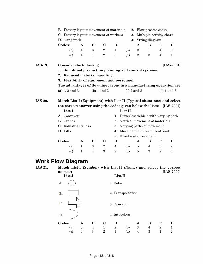
Work Flow Diagram IAS-21. Match List-I (Symbol) with List-II (Name) and select the correct
answer: [IAS-2000] List-I
List-II
1. Delay
2. Transportation
3. Operation
4. Inspection
Codes: A B C D A B C D (a) 3 4 1 2 (b) 3 4 2 1 (c) 4 3 2 1 (d) 4 3 1 2
Page 186 of 318

Layout Plant S K Mondal Chapter 9
IAS-22. A cutter breaks while cutting gears and is removed by the operator. Which of the following represents this activity on the flow process chart? [IAS-2004]
(a) Delay-D (b) Operation-O (c) Operation cum transportation-⇒ (d) inspection- IAS-23. What is a chart that shows the step-by-step procedure used, and the
interrelationship between anyone or more persons, forms or products when the procedure involves movement from place to place, called? [IAS-2007]
(a) Multi activity chart (b) Simo chart (d) Flow process chart – man analysis (d) Process chart – combined analysis
Computerized Techniques for Plant layout: CORELAP, CRAFT, ALDEP, PLANET, COFAD, CAN-Q IAS-24. Consider the following computer packages: [IAS-2001] 1. CORELAP 2. CRAFT 3. DYNAMO 4. SIMSCRIPT Which of these packages can be employed for layout analysis of
facilities? (a) 1 and 4 (b) 1 and 2 (c) 2 and 3 (d) 3 and 4
Page 187 of 318

Layout Plant S K Mondal Chapter 9
Answers with Explanation (Objective)
Previous 20-Years GATE Answers GATE-1. Ans. (d) In quadrant I, we can locate any one of
the four machines (i.e.) we can allocate quadrant I in 4 ways. Thereafter quadrant II in 3 ways, thereafter quadrant III in 2 ways. No further choice for quadrant IV.
∴ Total number of possible layouts = 4 × 3 × 2 = 24 GATE-2. Ans. Process GATE-3. Ans. (a) GATE-4. Ans. (a) GATE-5. Ans. (d)
Previous 20-Years IES Answers
IES-1. Ans. (c) IES-2. Ans. (c) IES-3. Ans. (b) IES-4. Ans. (d) Production, planning and control function are extremely complex in batch
production shop producing a batch at irregular intervals. IES-5. Ans. (c) IES-6. Ans. (d) IES-7. Ans. (a) IES-8. Ans. (a) IES-9. Ans. (c) IES-10. Ans. (b) IES-11. Ans. (c) IES-12. Ans. (a) Air cargo movements fall under fixed path system using conveyors. IES-13. Ans. (a) IES-14. Ans. (b) A diagram showing the path followed by men and materials while
performing a task is known as flow process chart. IES-15. Ans. (a) IES-16. Ans. (d) IES-17. Ans. (c) IES-18. Ans. (d)
Page 188 of 318

Layout Plant S K Mondal Chapter 9
Previous 20-Years IAS Answers IAS-1. Ans. (b) IAS-2. Ans. (c) IAS-3. Ans. (d) IAS-4. Ans. (d) IAS-5. Ans. (b) IAS-6. Ans. (d) A is false. Product layout has lowest flexibility. For flexibility in sequence
of operation use process layout. IAS-7. Ans. (d) IAS-8. Ans. (a) IAS-9. Ans. (c) R is false. Process layout does not have defined mathematical flow. That so
why material handling is costly and lot of back-tracking and cross-movements of work.
IAS-10. Ans. (d) IAS-11. Ans. (a) IAS-12. Ans. (b) IAS-13. Ans. (b) IAS-14. Ans. (b) IAS-15. Ans. (a) IAS-16. Ans. (c) IAS-17. Ans. (c) IAS-18. Ans. (a) IAS-19. Ans. (b) IAS-20. Ans. (b) IAS-21. Ans. (b) IAS-22. Ans. (b) IAS-23. Ans. (d) IAS-24. Ans. (b)
Page 189 of 318

10. Control Chart
Theory at a Glance (For IES, GATE, PSU) Control charts are statistical tool, showing whether a process is in control or not. It is a graphical tool for monitoring the activities of an ongoing process also referred as Shewhart control charts. Control charts are used for process monitoring and variability reduction.
Before discussing and calculating the limits etc. of control charts, it is necessary to understand causes of variations present in the system. Variability is an inherent feature of every process. Production data always have some variability.
Causes of Variations Two types of causes are present in the production system
• Special causes: Variation due to identifiable factors in the production process. Examples of special causes include: wrong tool, wrong production method, improper raw material, operator's skill, wrong die etc. Control of process is achieved through the elimination of special causes. According to Deming, only 15% of the problems are due to the special causes. Special causes or also sometimes referred as Assignable causes
• Common causes: Variation inherent in the process. Improvement of process is accomplished through the reduction of common causes and improving the system. According to Deming, 85% of the problems are due to the common causes.
Assignable causes are controlled by the use of statistical process charts.
Steps in constructing a control chart • Decide what to measure or count • Collect the sample data • Plot the samples on a control chart • Calculate and plot the control limits on the control chart • Determine if the data is in control • If non-random variation is present, discard the data (fix the problem) and recalculate
the control limits • When data are with in the control limits we leave the process assuming there are
only chance causes present
A process is in control IF • No sample points outside control limits • Most points near process average or center line • About equal number of points above and below the center line • Sample point are distributed randomly
Page 190 of 318

S
TyTw1.
2.
TyTh1.
2.
XCoIn vava
CeTh
S K Mo
Contr
ypes of Pwo types of Variabl
weight, t Attribut
defective
ypes of Che classifica Variabl
sigma ch Attribu
chart, U
X – Chaontrol char the x bar criable. In Rriable.
entre line, uhe formulae
iiX ==∑
meiX =
iR =Ri = rangXmax(i) = Xmin (i) =
ondal
ol Chart R
Process Df process dle: Continutime, tempete: Discretee items in a
Control Chtion of contrle charts: ahart for the
ute chats: a chart. For
art and rts for the chart the sa
R chart, the
upper contro used are as
1
n
iX
n=∑
ean of the thi
max ( )iXge of ith sammaximum vminimum v
Representin
Data data: uous data. erature, diame data. Thi lot, numbe
harts rol charts dare meant fo individual uare meant fremember [
R – Ch variable tyample mean sample ran
ol limit, lows following:
sample; h
min (iX−mple value of the value of the
Contr
ng Limits,
Things wemeter, etc. ings we cour of defects
depend uponor variable units for attribute[CPU]
hart ype of datans are plottnges are plo
wer control l
sampn =
)i
data in ith s data in ith s
rol Chart
Special Ca
e can meas
unt. Examp per item etc
n the type oftype of data
e type of da
a (X bar anted in orderotted in ord
limit for x b
ple size;
sample sample
t
auses, Com
sure. Exam
ples includec.
f data. a. X bar an
ata. p chart
nd R chartr to control der to contro
bar and R c
datthiX i=
Chap
mmon Caus
mple include
e number o
d R Chart,
, np chart,
s) the mean ol the varia
charts are c
ta
pter 10
ses
es length,
or percent
X bar and
c chart, u
value of a ability of a
calculated.
Page 191 of 318

Control Chart S K Mondal Chapter 10
1
g
ii
RR
g==∑
R = mean of g samples
1
g
ii
X
XX CL
g== =∑
(Centre line for X bar chart)
X = mean of mean of g samples g = number of samples
3σ= + xXUCL X xσ = standard deviation of samples
x nσσ =
2
Rd
σ = = estimate of standard deviation of population
d2 = parameter depends on sample size n
2
3 3σ= + = +X
RUCL X Xn n d
2XVCL X A R= + (Upper control limit for X bar chart)
22
3Ad n
= = Parameter depends on sample size
value of A2 can be directly obtained from the standard tables 2XLCL X A R= − (Lower control limit for X bar chart)
3 32
3 ,RRUCL R R R d dd
σ σ σ= + = =
34 4
2
3 where 1⎛ ⎞= = +⎜ ⎟
⎝ ⎠R
dUCL D R D Rd
(Upper control limit for R chart)
33 3
2
3 where 1⎛ ⎞= = −⎜ ⎟
⎝ ⎠R
dUCL D R D Rd
(Lower control limit for R chart)
Example: Mean values and ranges of data from 20 samples (sample size = 4) are shown in the table below:
Page 192 of 318

S
S N
1
2
3
4
Su
Av
Av
Up Lo Up Lo
XSathe
S K MoS.
No.
Mea
n of
Sa
mpl
e
1 10
2 15
3 12
4 11
um of mean
verage of me
verage of Ra
pper Contro
ower Contro
pper Contro
ower Contro
X-Bar Cample data ae special cau
ondal
Ran
ge
S. N
o.
4 5
4 6
5 7
4 8
of 20 sampl
ean values o
anges of 20 s
ol Limit of X
ol Limit of X ol Limit of R
ol Limit of R
Chart at S.N 2, 16uses and re
Mea
n of
Sa
mpl
e
Ran
ge
9 5
11 6
11 4
9 4
les = 20
1iX
=
=∑
of 20 sample
samples = i∑
X bar chart = =
X bar chart = =
R chart = D3
= 9.4R chart = D4
6, and 18 arvised limits
Contr
S. N
o.
Mea
n of
Sa
mpl
e
9 10
10 11
11 12
12 13
232=
es =
20
1
20i
X= =∑
20
1 4.1520
iR
= =∑
= 11.6 + A2 4= 14.63 = 11.6 – A2 4= 8.57
4.15 (D3 = 247 9.5
4.15 (D4 = 0
re slightly abs are advise
rol Chart
Sam
ple
Ran
ge
S. N
o.
4 13
6 14
5 15
4 16
11.6 (Cente
(Center Lin
4.15 (A2 = 0
4.15 (A2 = 0
2.282 for sa
0 for sample
bove the UCd to calcula
t
S. N
o.
Mea
n of
Sa
mpl
e
R
3 12 4
4 12 3
5 11 3
6 15 4
er Line of X
ne of R Char
0.729 for sam
.729 for sam
mple size 4)
e size 4)
CL. Efforts ate after dele
Chap
Ran
ge
S. N
o.
Mea
n of
4 17
3 18
3 19
4 20
X bar Chart)
rt)
mple size 4)
mple size 4)
)
must be maeting these
pter 10
Mea
n of
Sa
mpl
e
Ran
ge
12 4
15 3
11 3
10 4
ade to find data.
Page 193 of 318

Control Chart S K Mondal Chapter 10
R Chart All the data are within the LCL and UCL in R Chart. Hence variability of the process data is not an issue to worry.
C – Chart and P – Chart Control charts for Attribute type data (p, c, u charts) p-charts calculates the percent defective in sample. p-charts are used when observations can be placed in two categories such as yes or no, good or bad, pass or fail etc.
c-charts counts the number of defects in an item. c-charts are used only when the number of occurrence per unit of measure can be counted such as number of scratches, cracks etc.
u-chart counts the number of defect per sample. The u chart is used when it is not possible to have a sample size of a fixed size.
For attribute control charts, the estimate of the variability of the process is a function of the process average.
Centre line, upper control limit, lower control limit for c, p, and u charts are calculated. The formulae used are as following:
p-chart formulae Sum of defectivesspeice in all samplesTotal number of items in all samples
=p = centre line of p chart
(1 ) (1 )3 and 3− −= + = −
p p p pUCL p LCL pn n
Where n is the sample size. Sample size in p chart must be 50≥ Sometimes LCL in p chart becomes negative, in such cases LCL should be taken as 0
c-chart formulae
Sum of defects in all samples = Centre line of chart
Total number of samples
3 and 3
c c
UCL c c LCL c c
=
= + = −
Page 194 of 318

S
u-
ExDabe
S K Mo-chart f
STota
u =
ci = Numk = Numni = Size
UCL u=
xample: p-ata for defeelow:
Sample No.
1 2 3 4 5 6 7 8 9
10
SuSu
CL
UCL p
LCL p
=
=
=
ondal formula
Sum of defeal number o
mber of defecmber of sampe of ith samp
3 i
uun
+
-chart fective CDs
No. of DefectiveCDs = x
4 3 3 5 6 5 2 3 5 6
um of defectum of all sam
(13
(13
p ppn
p ppN
−+
−−
ae
ects in all saf items in a
cts in ith samples ples
and LCL
s from 20 s
e PropoDefec
x/samp0.00.00.00.00.00.00.00.00.00.0
tives 10 = mples 200
) 0.051
) 0.051
p
p
= +
= −
Contr
amples all samples
mple
3i
uL un
= −
samples (sa
ortion ctive = ple size
S
04 03 03 05 06 05 02 03 05 06
01 = 0.05100
0.051(1310
0.051(1310
−
−
rol Chart
1
1
=
k
iik
ii
c
n=
=
∑
∑
ample size
Sample No. D
C11 12 13 14 15 16 17 18 19 20
0.051) 000
0.051) 000
−=
−=
t
= 100) are
No. of Defective CDs = x
6 5 4 5 4 7 6 8 6 8
.066
.036
Chap
shown in
ProporDefecti
x/sample0.060.050.040.050.040.070.060.080.060.08
pter 10
the table
tion ve = e size 6 5 4 5 4 7 6 8 6 8
Page 195 of 318

S K
p-CSampspeciais imincreashow that d
ExamData table
SamNo
12345
=
=
CL
UCL
LCL =
C-CNone
K MonChart ple data at Sal causes anportant obsasing trend cyclic pattedata are notmple: c-ch for defect
e below:
mple o.
No.Defe
5 4
3 54 65 4
Sum of Number of109 = 5.4520
3 512.45
3 51.55 0
c c
c c
= + ==
= − == − =
Chart of the samp
ndal
S.N 16, 18, nd revised lservation th in the aver
ern. Processt from indepart ts on TV s
. of ects
SamN
5 64 75 86 94 1
defectsf samples
5
5.45 3 5.4
5.45 3 5.4
+
−
ple is out of
and 20 arelimits are ahat is clearrage propor appears to
pendent sou
et from 20
mple o.
NoDef
6 47 58 69 80 7
45
45
the LCL an
Control
e above the advised to carly visible
rtion defecti be out of co
urce.
0 samples
o. of fects
SamN
4 15 16 18 17 1
nd UCL. Bu
Chart
UCL. Efforalculate aftfrom the d
ives beyond ontrol and a
(sample si
mple No.
NoDef
11 12 13 14 15
t the chart
rts must beer deleting
data points sample nu
also there is
ize = 10) a
o. of fects
SamN
6 5 4 7 6
shows cyclic
Chapte
e made to fi these data. that therember15 als
s a strong ev
re shown
mple No.
NDe
16 17 18 19 20
c trend.
er 10
ind the . There e is an o, data vidence
in the
o. of efects
5 4 6 6 6
Page 196 of 318

Control Chart S K Mondal Chapter 10
OBJECTIVE QUESTIONS (GATE, IES, IAS)
Previous 20-Years GATE Questions
Quality Analysis and Control GATE-1. Statistical quantity control was developed by: [GATE-1995] (a) Frederick Taylor (b) Water shewhart (c) George Dantzig (d) W.E. Deming GATE-2. Match the following quantity control objective functions with the
appropriate statistical tools: [GATE-1992] Objective functions A. A casting process is to be controlled with
respect to hot tearing tendency B. A casting process is to be controlled with
respect to the number of blow holes, of any, produced per unit casting
C. A machining process is to be controlled with respect to the diameter of shaft machined
D. The process variability in a milling operation is to be controlled with respect to the surface finish of components
Statistical Tools P. X-chart Q. c-chart R. Random sampling S. p-chart T. Hypothesis testing
U. R-charts GATE-3. In a weaving operation, the parameter to be controlled is the
number of defects per 10 square yards of material. Control chart appropriate for, his task is: [GATE-1998]
(a) P-chart (b) C-chart (c) R-chart (d) X-chart
Previous 20-Years IES Questions
Quality Analysis and Control IES-1. Match List-I (Quality control concepts) with List-II (Quality control
techniques) and select the correct answer using the codes given below the lists: [IES-2004]
List-I List-II A. Tightened and reduced inspection 1. Dodge Romig tables B. Lot tolerance percent defective 2. Control chart for variables C. Poisson distribution 3. MIL standards D. Normal distribution 4. Control chart for number of
nonconformities Codes: A B C D A B C D (a) 2 1 4 3 (b) 3 4 1 2 (c) 3 1 4 2 (d) 2 4 1 3 IES-2. Quality control chart for averages was maintained for a dimension
of the product. After the control was established, it was found that the standard deviation (σ) of the process was 1.00 mm The
Page 197 of 318

Control Chart S K Mondal Chapter 10
dimension of the part is 70 ± 2.5 mm. Parts above 72.5 mm can be reworked but parts below 67.5 mm have to be scrapped. What should be the setting of the process to ensure production of no scrap and to minimize the rework? [IES-2004]
(a) 68.5 mm (b) 70 mm (c) 70.5 mm (d) 72.5 mm IES-3. The graph shows the results of
various quality levels for a component
Consider the following statements: 1. Curve A shows the variation of
value of component 2. Curve B shows the variation of
cost of the component 3. Graph is called as fish bone
diagram 4. The preferred level of quality is
given by line CC 5. The preferred level of quality is
given by line DD
[IES-2002] Which of the above statements are correct? (a) 1, 2 and 5 (b) 1, 3 and 4 (c) 2, 3 and 4 (d) 1, 2 and 4 IES-4. Match List-I (Scientist) with List-II (Research work) and select the
correct answer using the codes given below the lists: [IES-2000] List-I List-II A. Schewart 1. Less function in quality B. Taguchi 2. Queuing model C. Erlang 3. Zero defects 4. Control charts Codes: A B C A B C (a) 3 1 2 (b) 4 3 1 (c) 4 1 2 (d) 3 4 1 IES-5. Assertion (A): In case of Control Chart for fraction rejected (p-
chart), binomial distribution is used. [IES-2008] Reason (R): In binomial distribution probability of the event varies
with each draw. (a) Both A and R are true and R is the correct explanation of A (b) Both A and R are true but R is NOT the correct explanation of A (c) A is true but R is false (d) A is false but R is true IES-6. Assertion (A): In case of Control Charts for variables, the averages
of sub-groups of readings are plotted instead of plotting individual readings. [IES-2008]
Reason (R): It has been proved through experiments that averages will form normal distribution
(a) Both A and R are true and R is the correct explanation of A (b) Both A and R are true but R is NOT the correct explanation of A (c) A is true but R is false (d) A is false but R is true
Page 198 of 318

Control Chart S K Mondal Chapter 10
IES-7. Assertion (A): In case of control charts for variables, the average of readings of a subgroup of four and more is plotted rather than the individual readings. [IES-2000, 2003]
Reason (R): Plotting of individual readings needs a lot of time and effort.
(a) Both A and R are individually true and R is the correct explanation of A (b) Both A and R are individually true but R is not the correct explanation
of A (c) A is true but R is false (d) A is false but R is true IES-8. The span of control refers to the [IES-2003] (a) Total amount of control which can be exercised by the supervisor (b) Total number of persons which report to any- one supervisor (c) Delegation of authority by the supervisor to his subordinates (d) Delegation of responsibility by the supervisor to his subordinates IES-9. Consider the following statements: [IES-2001] Control chart of variables provides the
1. Basic variability of the quality characteristic. 2. Consistency of performance. 3. Number of products falling outside the tolerance limits.
Which of these statements are correct? (a) 1, 2 and 3 (b) 1 and 2 (c) 2 and 3 (d) 1 and 3 IES-10. Which one of the following steps would lead to interchangeability? (a) Quality control (b) Process planning [IES-1994] (c) Operator training (d) Product design IES-11. Match List-I (Trend/Defect) with List-II (Chart) and select the
correct answer using the codes given below the lists: [IES-2003] List-I List II A. Trend 1. R-Chart B. Dispersion 2. C-Chart C. Number of defects 3. X -Chart D. Number of defectives 4. np-Chart 5. u-Chart Codes: A B C D A B C D (a) 5 3 2 4 (b) 3 1 4 2 (c) 3 1 2 4 (d) 3 4 5 2 IES-12. Assertion (A): In case of control charts for variables, if some points
fall outside the control limits, it is concluded that the process is not under control. [IES-1999]
Reason (R): It was experimentally proved by Shewhart that averages of four or more consecutive readings from a universe (population) or from a process, when plotted, will form a normal distribution curve.
(a) Both A and R are individually true and R is the correct explanation of A (b) Both A and R are individually true but R is not the correct explanation
of A (c) A is true but R is false (d) A is false but R is true
Page 199 of 318

Control Chart S K Mondal Chapter 10
IES-13. Consider the following statements with respect to control charts for
attributes: [IES-2004] 1. The lower control limit is non-negative 2. Normal distribution is the order for this data 3. The lower control limit is not significant 4. These charts give the average quality characteristics
Which of the statements given above are correct? (a) 1, 2 and 3 (b) 2, 3 and 4 (c) 1, 3 and 4 (d) 1, 2 and 4 IES-14. If in a process on the shop floor, the specifications are not met, but
the charts for variables show control, then which of the following actions should be taken? [IES-2009]
(a) Changes the process (b) Change the method of measurement (c) Change the worker or provide him training (d) Change the specifications or upgrade the process
Page 200 of 318

Control Chart S K Mondal Chapter 10
Answers with Explanation (Objective)
Previous 20-Years GATE Answers GATE-1. Ans. (b) Dr. Waher Shewhart an American scientist during World War-II. GATE-2. Ans. A – S, B – Q, C – P, D – U GATE-3. Ans. (b)
Previous 20-Years IES Answers IES-1. Ans. (c) IES-2. Ans. (c) Standard deviation from mean = 0.5 mm Therefore for no scrap D = 70 + 0.5 = 70.5 mm IES-3. Ans. (c) IES-4. Ans. (c) IES-5. Ans. (c) IES-6. Ans. (a) IES-7. Ans. (b) IES-8. Ans. (d) IES-9. Ans. (a) IES-10. Ans. (a) Quality control leads to interchangeability. IES-11. Ans. (c) IES-12. Ans. (b) IES-13. Ans. (c) IES-14. Ans. (c)
Page 201 of 318

11. Sampling, JIT, TQM, etc.
Theory at a Glance (For IES, GATE, PSU)
Process Capability Process capability compares the output of an in-control process to the specification limits by using capability indices.
Capability Indices: A process capability index uses both the process variability and the
process specifications to determine whether the process is ‘capable’.
Capable Process: A capable process is one where almost all the measurements fall inside
the specification limits. This can be represented pictorially by the plot below.
Work Sampling Curve of normal distribution
To make things easier we speak 95% confidence level than 95.45%.
Remember:
Page 202 of 318

Sampling, JIT, TQM, etc. S K Mondal Chapter 11
95% confidence level or 95% of the area under the curve = 1.96
99% confidence level or 99% of the area under the curve = 2.58
99.9% confidence level or 99.9% of the area under the curve = 3.3
Standard error of proportion ( pσ ) = pqn
Where, p = percentage of idle time
q = percentage of working time = (1 – p)
n = number of observation
So you may use this equation as ( pσ ) = (1 )p pn− also.
Page 203 of 318

Sampling, JIT, TQM, etc. S K Mondal Chapter 11
OBJECTIVE QUESTIONS (GATE, IES, IAS)
Previous 20-Years GATE Questions
Sampling Plan (Single, Double, Sequential Sampling Plan) GATE-1. In carrying out a work sampling study in a machine shop, it was
found that a particular lathe was down for 20% of the time. What would be the 95% confidence interval of this estimate if 100 observations were made? [GATE-2002]
(a) 0.16, 0.24 (b) 0.12, 0.28 (c) 0.08, 0.32 (d) None of these GATE-2. Preliminary work sampling studies show that machine was idle 25%
of the time based on a sample of 100 observations. The number of observations needed for a confidence level of 95% and an accuracy of ± 5% is: [GATE-1996]
(a) 400 (b) 1200 (c) 3600 (d) 4800
Just in Time (JIT) GATE-3. List-I List-II [GATE-1995] (Problem areas) (Techniques) A. JIT 1. CRAFT B. Computer assisted layout 2. PERT C. Scheduling 3. Johnson's rule D. Simulation 4. Kanbans 5. EOQ rule 6. Monte Carlo
Previous 20-Years IES Questions
Process Capability IES-1. Which one of the following correctly explains process capability? (a) Maximum capacity of the machine [IES-1998] (b) Mean value of the measured variable (c) Lead time of the process (d) Maximum deviation of the measured variables of the components IES-2. Process capability of a machine is defined as the capability of the
machine to: [IES-1993] (a) Produce a definite volume of work per minute (b) Perform definite number of operations (c) Produce job at a definite spectrum of speed (d) Hold a definite spectrum of tolerances and surface finish
Operation Characteristic Curve (OC Curve)
Page 204 of 318

Sampling, JIT, TQM, etc. S K Mondal Chapter 11
IES-3. Match List-I with List-II and select the connect answer using the codes given below the lists: [IES-2001]
List-I List-II A. OC Curve 1. Acceptance sampling B. AOQL 2. Dodge Roming table C. Binomial distribution 3. p-charts D. Normal curve 4. Control charts for variables Codes: A B C D A B C D (a) 1 2 3 4 (b) 1 3 2 4 (c) 4 2 3 1 (d) 4 3 2 1 IES-4. The curve representing the level of achievement with reference to
time is known as [IES-2002] (a) Performance curve (b) Operating characteristic curve (c) S-curve (d) Learning curve IES-5. An operating characteristic curve (OC curve) is a plot between (a) Consumers’ risk and producers' risk [IES-2009] (b) Probability of acceptance and probability of rejection (c) Percentage of defective and probability of acceptance (d) Average outgoing quality and probability of acceptance
Sampling Plan (Single, Double, Sequential Sampling Plan) IES-6. Assertion (A): Double sampling is preferred over single sampling
when the quality or incoming lots is expected to be either very good or very bad. [IES-2000]
Reason (R): With double sampling, the amount of inspection required will be lesser than that in the case of single sampling.
(a) Both A and R are individually true and R is the correct explanation of A (b) Both A and R are individually true but R is not the correct explanation
of A (c) A is true but R is false (d) A is false but R is true IES-7. Which one of the following statements is not correct? [IES-2008] (a) The operating characteristic curve of an acceptance sampling plan shows
the ability of the plan to distinguish between good and bad lots. (b) No sampling plan can give complete protection against the acceptance of
defective products. (c) C-chart has straight line limits and U chart has zig-zag limits. (d) Double sampling results in more inspection than single sampling if the
incoming quality is very bad. IES-8. Which one of the following is not the characteristic of acceptance
sampling? [IES-2007] (a) This is widely suitable in mass production (b) It causes less fatigue to inspectors (c) This is much economical (d) It gives definite assurance for the conformation of the specifications for
all the pieces IES-9. Assertion (A): Sampling plans with acceptance number greater than
zero are generally better than sampling plans with acceptance number equal to zero. [IES-2006]
Page 205 of 318

Sampling, JIT, TQM, etc. S K Mondal Chapter 11
Reason (R): Sampling plans with acceptance number greater than zero have a larger sample size as compared to similar sampling plans with acceptance number equal to zero.
(a) Both A and R are individually true and R is the correct explanation of A (b) Both A and R are individually true but R is not the correct explanation
of A (c) A is true but R is false (d) A is false but R is true IES-10. Assertion (A): In attribute control of quality by sampling, the sample
size has to be larger than variable control. [IES-2005] Reason (R): Variables are generally continuous, and attributes have
few discrete levels. (a) Both A and R are individually true and R is the correct explanation of A (b) Both A and R are individually true but R is not the correct explanation
of A (c) A is true but R is false (d) A is false but R is true IES-11. Consider the following statements in respect of double sampling
plan: [IES-2003] 1. Average number of pieces inspected is double that of single
sampling 2. Average number of pieces inspected is less than that for single
sampling 3. Decision to accept or reject the lot is taken only after the
inspection of both samples 4. Decision to accept or reject the lot is reached sometimes after
one sample and sometimes after two samples Which of these statements are correct? (a) 1, 2 and 3 (b) 2 and 4 (c) 1 and 4 (d) 2 and 3 IES-12. Assertion (A): In dodge romig sampling tables, the screening
inspection of rejected lots is also included. [IES-2001] Reason (R): Dodge romig plans are indexed at an LTPD of 10% (a) Both A and R are individually true and R is the correct explanation of A (b) Both A and R are individually true but R is not the correct explanation
of A (c) A is true but R is false (d) A is false but R is true IES-13. The product is assembled from parts A and B. The probability of
defective parts A and B are 0.1 and 0.2 respectively. Then the probability of the assembly of A and B to be non defective is:
[IES-1992] (a) 0.7 (b) 0.72 (c) 0.8 (d) 0.85 IES-14. A control chart is established with limits of ± 2 standard errors for
use in monitoring samples of size n = 20. Assume the process to be in control. What is the likelihood of a sample mean falling outside the control limits? [IES-2005]
(a) 97.7% (b) 95.5% (c) 4.5% (d) 2.3% IES-15. In a study to estimate the idle time of a machine, out of 100 random
observations the machine was found idle on 40 observations. The
Page 206 of 318

Sampling, JIT, TQM, etc. S K Mondal Chapter 11
total random observations required for 95% confidence level and ± 5% accuracy is: [IES-2001]
(a) 384 (b) 600 (c) 2400 (d) 9600 IES-16. The management is interested to know the percentage of idle time
of equipment. The trial study showed that percentage of idle time would be 20%. The number of random observations necessary for 95% level of confidence and ± 5% accuracy is: [IES-2000]
(a) 6400 (b) 1600 (c) 640 (d) 160 IES-17. If one state occurred four times in hundred observations while
using the work-sampling technique, then the precision of the study using a 95% confidence level will be: [IES-1997]
(a) 90% (b) 92% (c) 95% (d) 98% IES-18. For a confidence level of 95% and accuracy ± 5%, the number of
cycles to be timed in a time study is equal to: [IES-2009]
22 2( )N X Xk
X⎡ ⎤∑ − ∑⎢ ⎥
∑⎢ ⎥⎣ ⎦
Where, N = Number of observations taken; X = X1, X2, ...., XN are individual observations. What is the value of K?
(a) 10 (b) 20 (c) 30 (d) 40
Previous 20-Years IAS Questions
Just in Time (JIT) IAS-1. Match List-I with List-II and select the correct answer: [IAS-2000] List-I A. Just-in-time inventory and
procurement techniques B. Work-in-progress likely to be low
compared to output C. Scheduling typically most
complex processes D. Flexible manufacturing cell
List-II 1. Intermittent production 2. Repetitive production 3. Continuous production 4. Job production
Codes: A B C D A B C D (a) 2 3 4 1 (b) 3 2 1 4 (c) 2 3 1 4 (d) 3 2 4 1
Page 207 of 318

S K
An
GATE
GATE
GATE
IES-1IES-2
IES-3IES-4IES-5
IES-6IES-7IES-8IES-9IES-1IES-1IES-1IES-1
IES-1
IES-1
K Mon
nswe
PrE-1. Ans. (b
E-2. Ans. (d
Wh Nuis:
E-3. Ans. (a
P1. Ans. (d) 2. Ans. (d) P
to h3. Ans. (a) 4. Ans. (a) 5. Ans. (
Ch∴
6. Ans. (d) 7. Ans. (d) 8. Ans. (d) 9. Ans. (d) 10. Ans. (a)11. Ans. (b)12. Ans. (b)13. Ans. (b)
nonProHe= 0
14. Ans. (c)
15. Ans. (c)
ndal
rs wi
reviousb)
d) S P K× =
here, K S P
umber of ob
2(K PNS
=
a) – 4, (B) –
Previou
Process caphold a defin
(c) OC Characteristic
OC CURbetween defective aacceptance
) ) ) ) It is a casen-defective obability th
ence, probab0.72.
1.96 5pσ =
Samp
ith Ex
s 20-Y
(1 )P PKN−
= 2 for 95= 0.05 (ac= 0.25 (idservations
2 2) (1 ) (2P
S P−
=
1, (C) – 3, (
us 20-Y
pability of a nite spectrum
Curve (Opec Curve) RVE is a
percentagand probabe.
e of mutuall= 1 – 0.1 = 0
hat Part-B isbility that b
or, 2pσ =
pling, JIT
xplan
Years G
5% confidencccuracy) dle time) needed for
2
22) (0.25)(1
(0.05) (0.−
(D) – 6
Years
machine is m of toleran
erating
a plot ge of bility of
ly independ0.9 s non-defectboth Part-A
40 62.5n×
=
T, TQM,
nation
GATE A
ce level
95% confide
20.25) 48
25)−
=
IES A
defined as nces and sur
ent events.
tive, = 1 – 0. and Part-B
60 or, 3n ≈
etc.
n (Obj
Answe
ence level a
00
Answer
the capabilrface finish.
Probability
.2 = 0.8 B are non-de
384
Chapte
jectiv
ers
and ± 5% ac
rs
ity of the m.
y that the pa
efective = 0.
er 11
ve)
ccuracy
machine
art A is
9 × 0.8
Page 208 of 318

Sampling, JIT, TQM, etc. S K Mondal Chapter 11
IES-16. Ans. (a) 20 801.96 5 or, 2.5 or, 160p p nn
σ σ ×= = = ≈
IES-17. Ans. (d) Accuracy = (1 )p pN− for 95% confidence level = 0.05 0.95 0.02 2%
100×
≈ =
∴ Precision = 98% IES-18. Ans. (d) For 95% confidence level K = 2 S = Accuracy = 0.05 2 40
0.05KKS
= = =
Previous 20-Years IAS Answers IAS-1. Ans. (a)
Conventional Questions with Answer Conventional Question [ESE-2007] From the data of a pilot study, the percentage of occurrence of an activity is
60%. Find the number of observations for 95% confidence level and an accuracy of ± 2%. [2 Marks]
Solution: The formulae for determining the number of observations is
( )
pp 1 p
S KN−
=
or ( )2
2p
p 1 pN K
S−
= where
S = the desired relative accuracy ( )2% 0.02± = ± pS = the desired absolute accuracy P = percentage accuracy of an activity of interest or a classification being measured. (60% = 0.6) N = total number of random observations.
( )
( )
2
22 0.6 1 0.6
N0 0.02 0.6× −
∴ =± ×
( )2
4 0.6 0.40.012
× ×=
±
0.96 66670.000144
=+
Page 209 of 318

12. Graphical Method
Theory at a Glance (For IES, GATE, PSU)
What is LPP (Q-ESE) Linear programming is a technique which allocates scare available resources under conditions of certainty in an optimum manner, (i.e. maximum or minimum) to achieve the company objectives which may be maximum overall profit or minimum overall cost.
Linear programming deals with the optimization (maximization or minimization) of linear functions subjects to linear constraints.
One L.P.P Maximize (z) = 3x1 + 4x2 (i) Subject to 4x1 + 2x2 ≥ 80 (ii) 2x1 + 5x2 ≤ 180 (iii) x1, x2 ≥ 0 (iv) 1. The variables that enter into the problem are called decision variables. e.g., x1, x2. 2. The expression showing the relationship between the manufacture's goal and the
decision variables is called the objective function. e.g. z = 3x1 + 4x2 (maximize). 3. The inequalities (ii); (iii); (iv) are called constraints being all linear, it is a linear
programming problem (L.P.P).This is an example of a real situation from industry.
Graphical Method Working Procedure: Step-1: Formulate the given problem as a linear programming problem. Step-2: Plot the given constraints as equalities on x1.x2 co-ordinate plane and determine
the convex region formed by them.
[A region or a set of points is said to be convex if the line joining any two of its points lies completely in the region (or the set)]
Step-3: Determine the vertices of the convex region and find the value of the objective function and find the value of the objective function at each vertex. The vertex which gives the optimal value of the objective function gives the desired optimal solution the problem.
Otherwise: Draw a dotted line through the origin representing the objective function with z = 0. As z is increased from zero, this line moves to the right remaining parallel to itself. We go on sliding this line (parallel to itself), till it is farthest away from the origin and passes through only one vertex on the convex region. This is the vertex where the maximum value of z is attained. When it is required to minimize zn value z is increased till the dotted line passes through the nearest vertex of the convex region. Example: Maximize z = 3x1 + 4x2
Page 210 of 318
Graphical Method S K Mondal Chapter 12
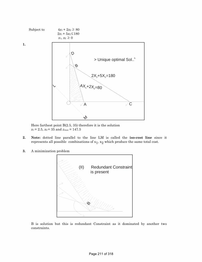
Subject to 4x1 + 2x2 ≥ 80 2x1 + 5x2≤180 x1, x2 ≥ 0
1.
Here farthest point B(2.5, 35) therefore it is the solution x1 = 2.5, x2 = 35 and zmax = 147.5 2. Note: dotted line parallel to the line LM is called the iso-cost line since it
represents all possible combinations of x1, x2 which produce the same total cost. 3. A minimization problem
B is solution but this is redundant Constraint as it dominated by another two constraints.
L
M
D
B
2X +5X =1802 2
AX +2X =801 2
A C
> Unique optimal Sol..h
B
(II) Redundant Constraint is present
Page 211 of 318

Graphical Method S K Mondal Chapter 12
4.
5.
6.
Here the constraints were incompatible. So, there is no solution.
LMIIAB So infinite number of sol..”
L
M
It is a maximization problem:but region is not bounded soHere Unbounded Sol..”
Page 212 of 318

Graphical Method S K Mondal Chapter 12
OBJECTIVE QUESTIONS (GATE, IES, IAS)
Previous 20-Years GATE Questions GATE-1. The first algorithm for Linear Programming was given by:
[GATE-1999] (a) Bellman (b) Dantzig (c) Kulm (d) Van Neumann GATE-2. If at the optimum in a linear programming problem, a dual variable
corresponding to a particular primal constraint is zero, then it means that [GATE-1996]
(a) Right hand side of the primal constraint can be altered without affecting the optimum solution
(b) Changing the right hand side of the primal constraint will disturb the optimum solution
(c) The objective function is unbounded (d) The problem is degenerate GATE-3. Consider the following Linear Programming Problem (LPP): Maximize z = 3x1 + 2x2 [GATE -2009] Subject to x1 ≤ 4 x2 ≤ 6 3x1 + x2 ≤ 18 x2 ≥ 0, x2 ≥ 0
(a) The LPP has a unique optimal solution (b) The LPP is infeasible (c) The LPP is unbounded (d) The LPP has multiple optimal solutions.
Graphical Method GATE-4. A manufacturer produces two types of products, 1 and 2, at
production levels of x1 and x2 respectively. The profit is given is 2x1 + 5x2. The production constraints are: [GATE-2003]
1 23 40x x+ ≤ 1 23 24x x+ ≤ 1 2 10x x+ ≤ 1 20, 0x x> > The maximum profit which can meet the constraints is: (a) 29 (b) 38 (c) 44 (d) 75 Statement for Linked Answer Questions Q5 and Q6: Consider a linear programming problem with two variables and two constraints. The objective function is: Maximize X1+ X2. The corner points of the feasible region are (0, 0), (0, 2) (2, 0) and (4/3, 4/3) [GATE-2005] GATE-5. If an additional constraint X1 + X2 ≤ 5 is added, the optimal solution
is:
Page 213 of 318

Graphical Method S K Mondal Chapter 12
(a) 5 5,3 3⎛ ⎞⎜ ⎟⎝ ⎠
(b) 4 4,3 3
⎛ ⎞⎜ ⎟⎝ ⎠
(c) 5 5,2 2⎛ ⎞⎜ ⎟⎝ ⎠
(d) (5, 0)
GATE-6. Let Y1 and Y2 be the decision variables of the dual and v1 and v2 be
the slack variables of the dual of the given linear programming problem. The optimum dual variables are:
(a) Y1 and Y2 (b) Y1 and v1 (c) Y1 and v2 (d) v1 and v2
Previous 20-Years IES Questions IES-1. Which one of the following is the correct statement? [IES-2007] In the standard form of a linear programming problem, all
constraints are: (a) Of less than or equal to, type. (b) Of greater or equal to, type. (c) In the form of equations. (d) Some constraints are of less than equal to, type and some of greater than
equal to, type. IES-2. Match List-I with List-II and select the correct answer using the
codes given below the lists: [IES-1995] List-I List-II A. Linear programming 1. Ritchie B. Dynamic programming 2. Dantzig C. 'C' programming 3. Bell D. Integer programming 4. Gomory Codes: A B C D A B C D (a) 2 1 4 3 (b) 1 2 3 4 (c) 2 3 1 4 (d) 2 3 4 1 IES-3. A feasible solution to the linear programming problem should (a) Satisfy the problem constraints [IES-1994] (b) Optimize the objective function (c) Satisfy the problem constraints and non-negativity restrictions (d) Satisfy the non-negativity restrictions IES-4. Consider the following statements: [IES-1993] Linear programming model can be applied to: 1. Line balancing problem 2. Transportation problem 3. Project management Of these statements: (a) 1, 2 and 3 are correct (b) 1 and 2 are correct (c) 2 and 3 are correct (d) 1 and 3 are correct. IES-5. Solution to Z = 4x1 + 6x2 [IES-1992] 1 2 1 2 1 24; 3 12; , 0 is:x x x x x x+ ≤ + ≤ ≥ (a) Unique (b) Unbounded (c) Degenerate (d) Infinite IES-6. The primal of a LP problem is maximization of objective function
with 6 variables and 2 constraints. [IES-2002]
Which of the following correspond to the dual of the problem stated?
Page 214 of 318

Graphical Method S K Mondal Chapter 12
1. It has 2 variables and 6 constraints 2. It has 6 variables and 2 constraints 3. Maximization of objective function 4. Minimization of objective function Select the correct answer using the codes given below: (a) 1 and 3 (b) 1 and 4 (c) 2 and 3 (d) 2 and 4
Graphical Method IES-7. In a linear programming problem, which one of the following is
correct for graphical method? [IES-2009] (a) A point in the feasible region is not a solution to the problem (b) One of the corner points of the feasible region is not the optimum
solution (c) Any point in the positive quadrant does not satisfy the non-negativity
constraint (d) The lines corresponding to different values of objective functions are
parallel IES-8. In case of solution of linear programming problem using graphical
method, if the constraint line of one of the non-redundant constraints is parallel to the objective function line, then it indicates [IES-2004, 2006]
(a) An infeasible solution (b) A degenerate solution (c) An unbound solution (d) A multiple number of optimal
solutions IES-9. Which of the following are correct in respect of graphically solved
linear programming problems? [IES-2005] 1. The region of feasible solution has concavity property. 2. The boundaries of the region are lines or planes. 3. There are corners or extreme points on the boundary
Select the correct answer using the code given below: (a) 1 and 2 (b) 2 and 3 (c) 1 and 3 (d) 1, 2 and 3 IES-10. Which one of the following statements is NOT correct? [IES-2000] (a) Assignment model is a special ease of a linear programming problem (b) In queuing models, Poisson arrivals and exponential services are
assumed (c) In transportation problems, the non-square matrix is made square by
adding a dummy row or a dummy column (d) In linear programming problems, dual of a dual is a primal IES-11. Consider the following statements regarding the characteristics of
the standard form of a linear programming problem: [IES-1999] 1. All the constraints are expressed in the form of equations. 2. The right-hand side of each constraint equation is non-negative. 3. All the decision variables are non-negative.
Which of these statements are correct? (a) 1, 2 and 3 (b) 1 and 2 (c) 2 and 3 (d) 1 and 3
Page 215 of 318

Graphical Method S K Mondal Chapter 12
IES-12. A variable which has no physical meaning, but is used to obtain an
initial basic feasible solution to the linear programming problem is referred to as: [IES-1998]
(a) Basic variable (b) Non-basic variable (c) Artificial variable (d) Basis IES-13. Which of the following conditions are necessary of applying linear
programming? [IES-1992] 1. There must be a well defined objective function 2. The decision variables should be interrelated and non-negative 3. The resources must be in limited supply (a) 1 and 2 only (b) 1 and 3 only (c) 2 and 3 only (d) 1, 2 and 3 IES-14. If m is the number of constraints in a linear programming with two
variables x and y and non-negativity constraints x ≥ 0, y ≥ 0; the feasible region in the graphical solution will be surrounded by how many lines? [IES-2007]
(a) m (b) m + 1 (c) m + 2 (d) m + 4 IES-15. Consider the following linear programming problem: [IES-1997] Max. Z = 2A + 3B, subject to A + B < 10, 4A + 6B < 30, 2A + B < 17, A, B ≥ 0. What can one say about the solution? (a) It may contain alternative optima (b) The solution will be unbounded (c) The solution will be degenerate (d) It cannot be solved by simplex method
Page 216 of 318

Graphical Method S K Mondal Chapter 12
Answers with Explanation (Objective)
Previous 20-Years GATE Answers GATE-1. Ans. (b) GATE-2. Ans. (c) GATE-3. Ans. (a)
GATE-4. Ans. (a) Rearranging the above equations 1 2 140403
x x+ ≤⎛ ⎞⎜ ⎟⎝ ⎠
, 1 2 18 24x x
+ ≤ and
1 2 1.x x+ ≤ Draw the lines and get solution.
GATE-5. Ans. (b) GATE-6. Ans. (d)
Previous 20-Years IES Answers
IES-1. Ans. (c) IES-2. Ans. (c) IES-3. Ans. (c) A feasible solution to the linear programming problem should satisfy the
problem constraints. IES-4. Ans. (b) Linear programming model can be applied to line balancing problem and
transportation problem but not to project management. IES-5. Ans. (a) 1 2
1 2
1 1 2
43 122 8 4 and 0
X XX XX X X
+ =
+ =
− = − ⇒ = =
IES-6. Ans. (b) IES-7. Ans. (a) IES-8. Ans. (d) All points on the line is a solution. So there are infinite no of optimal
solutions. IES-9. Ans. (b) IES-10. Ans. (c) IES-11. Ans. (a) IES-12. Ans. (c) IES-13. Ans. (d)
Page 217 of 318

Graphical Method S K Mondal Chapter 12
IES-14. Ans. (c) Constraints = 3 the feasible region is surrounded by more two lines x-axis and y-axis.
IES-15. Ans. (a)
Page 218 of 318

Graphical Method S K Mondal Chapter 12
Conventional Questions with Answer Conventional Question [ESE-2007] Two product A and B are to be machined on three machine tools, P, Q and R.
Product A takes 10 hrs on machine P, 6 hrs on machine Q and 4 hrs on machine R. The product B takes 7.5 hrs on machine P, 9 hrs on machine Q and 13 hrs on machine R. The machining time available on these machine tools, P, Q, R are respectively 75 hrs, 54 hrs and 65 hrs per week. The producer contemplates profit of Rs. 60 per product A, and Rs. 70 per product B. Formulate LP model for the above problem and show the feasible solutions to the above problem? Estimate graphically/ geometrically the optimum product mix for miximizing the profit. Explain why one of the vertics of the feasible region becomes the optimum solution point.
(Note: Graph sheet need not be used) [15-Marks] Solution: The given data are tabulated as follows:
Let = number of A to be machined
= number of B to be machined, for profit maximization. Problem formulation: (i) Restriction on availability of machines for operation. (a) If only A were operated on machine P Then,
(b) If only B were operated on machine P then, Since, both A and B are operated on machine P … (i)
Similarly, … (ii)
And … (iii) Now, profit equation: Profit fper product A = Rs.60 and profit per product B = Rs. 70 ∴Total profit is ∴Objective function which is to be maximized is
1x
2x
1x 75 / 10≤
110x 75≤
27.5x 75≤
1 210x 7.5x 75∴ + ≤
1 26x 9x 54+ ≤
1 25x 13x 65+ ≤
1 260x 70x+
1 2Z 60x 70x= +
Machine No. Time taken for operation on A
Time taken for operation on B
Available hours per week
P 10 7.5 75 Q 6 9 54 R 5 13 65
Page 219 of 318

Graphical Method S K Mondal Chapter 12
|
|
|
|
|
|
|
|
|
|
|
|
|
|
|
|
|
|
||
|
||
|
x2
x1
(0,5)
(0,6)
(0,10)
(13,0)
(9,0)(7.5,0)D••
•
•
C
BA
0
(i)
(ii)(iii)
OABCD in the graph is feasible reagion On solving equation (ii) and (iii) we get co-ordinates of B ( )B 3.5454,3.6363∴ ≡ On solving equation (i) and (ii) we get co-ordinates of C ( )C 6,2∴ ≡
And ( )A 0,5≡ ; ( )D 7.5,0≡ Now, ( )Z A 60 0 70 5 350= × + × =
( )Z B 60 3.5454 70 3.6363 467.265= × + × =
( )Z C 60 6 70 2 500= × + × =
( )Z D 60 7.5 70 0 450= × + × = Hence optimum solution is A = 6 and B = 2
Page 220 of 318

13. Simplex Method
Theory at a Glance (For IES, GATE, PSU)
General Linear Programming Problem Optimize {Minimize or maximize} 1 1 2 2 3 3 1 1.........Z c x c x c x c x= + + + +
Subjected to the constraints a11x1 + a12x2 + ...... + a1xxn ≤ b1 a21x1 + a22x2 + ...... + a2xxn ≤ b2 ------------------------------------------------------- ------------------------------------------------------- am1x1 + am2x2 + ...... + axmnxn ≤ bm
and meet the non-negativity restrictions x1, x2, x3, ...... xn ≥ 0 1. A set of values x1, x2, x3, ...... xn which constrains of the L.P.P. is called its solutions. 2. Any solution to a L.P.P. which satisfies the non-negativity restrictions of the problem
is called its feasible Solution. 3. Any feasible solution which maximizes (or minimizes) the objective function of the
L.P.P. is called its optimal solution. 4. A constraints
1
1
,( 1,2,........ )
,( 1,2,.... )
n
ij i ij
n
ij i i ij
a x b i m
a x s b i m
=
=
≤ =
+ = =
∑
∑
Then the si is called slack variables.
5. A constraints
1
1
,( 1,2,........ )
,( 1,2,.... )
n
ij i ij
n
ij i i ij
a x b i m
a x s b i m
=
=
≥ =
− = =
∑
∑
Then the Si is called surplus variables.
6. Canonical forms of L.P.P. Maximize z = c1x1 + c2x2 + ................ + cnxn
Subject to the Constraints ai1x1 + ai2x2 + ...... + ainxn ≤ bi; [i = 1, 2, .... m] x1, x2, ........, xn ≥ 0
7. Standard from of L.P.P Maximize z=c1x1+ c2x2+....+cnxn Subject to the constraint ai1x1 + ai2x2 + ...... + ainxn ≤ bi [i = 1, 2, .. m] x1, x2, ......, xn ≥ 0 8. Convert the following L.PP. to the standard form Maximize 1 2 33 5 7z x x x= + +
Page 221 of 318

Simplex Method S K Mondal Chapter 13
Subject to 1 26 4 5x x− ≤ 1 2 33 2 5 11x x x+ + ≥ 1 34 3 2x x+ ≤ 1 2, ..... 0x x ≥ As x3 is unrestricted let 3 3 3 ' ''x x x= − Where 3 3', ''x x And Introducing the slack/surplus variables, the problem in standard form becomes: Maximize 3 1 2 3 35 7 ' 7 "z x x x x+ + − Subject to 1 2 36 4 5 5x x x− + = 1 2 3 3 23 2 5 5 11x x x x s′ ′′+ + − − = 1 3 3 34 3 3 2x x x s′ ′′+ − − = ' "
1 2 3 3 1 2 3, , , ; , , 0x x x x s s s ≥
Big-M Method In the simplex method was discussed with required transformation of objective function and constraints. However, all the constraints were of inequality type withless-than-equal-to’ (δ) sign. However, ‘greater-than-equal-to’ (ε) and ‘equality’ (=) constraints are also possible. In such cases, a modified approach is followed, which will be discussed in this chapter. Different types of LPP solutions in the context of Simplex method will also be discussed. Finally, a discussion on minimization vs maximization will be presented.
Simplex method with ‘greater-than-equal-to’ (ε�) and equality (=) constraints The LP problem, with ‘greater-than-equal-to’ (ε) and equality (=) constraints, is transformed to its standard form in the following way :
1. One ‘artificial variable’ is added to each of the ‘greater-than-equal-to’ (ε) and equality (=) constraints to ensure an initial basic feasible solution.
2. Artificial variables are ‘penalized’ in the objective function by introducing a large negative (positive) coefficient M for maximization (minimization) problem.
3. Cost coefficients, which are supposed to be placed in the Z-row in the initial simplex tableau, are transformed by ‘pivotal operation’ considering the column of artificial variable as ‘pivotal column’ and the row of the artificial variable as ‘pivotal row’.
4. If there are more than one artificial variable, step 3 is repeated for all the artificial variables one by one.
Let us consider the following LP problem Maximize 1 23 5Z x x= + Subject to 1 2 2x x+ ≥
2
1 2
1 2
63 2 18
, 0
xx x
x x
≤
+ =
≥
After incorporating the artificial variables, the above LP problem becomes as follows: Maximize 1 2 1 23 5Z x x Ma Ma= + − − Subject to 1 2 3 1 2x x x a+ − + =
Page 222 of 318

Simplex Method S K Mondal Chapter 13
2 4
1 2 2
1 2
63 2 18
, 0
x xx x a
x x
+ =
+ + =
≥
Where x3 is surplus variable, x4 is slack variable and a1 and a2 are the artificial variables. Cost coefficients in the objective function are modified considering the first constraint as follows:
1 2 3 1 2(3 4 ) (5 3 ) 0 0 20 MZ M x M x Mx a a− + − + + + + = − The modified cost coefficients are to be used in the Z-row of the first simplex tableau.
Next, let us move to the construction of simplex tableau. Pivotal column, pivotal row and pivotal element are marked (same as used in the last class) for the ease of understanding.
Note: That while comparing (– 3 – 4M) and (– 5 – 3M), it is decided that (– 3 – 4M) <
(– 5 – 3M) as M is any arbitrarily large number.
Successive iterations are shown as follows:
Page 223 of 318

Simplex Method S K Mondal Chapter 13
It is found that, at iteration 4, optimality has reached. Optimal solution is Z = 36 with x1 = 2 and x2 = 6. The methodology explained above is known as Big-M method. Hope, reader has already understood the meaning of the terminology!
‘Unbounded’, ‘Multiple’ and ‘Infeasible’ solutions in the context of Simplex Method As already discussed in lecture notes 2, a linear programming problem may have different type of solutions corresponding to different situations. Visual demonstration of these
Page 224 of 318

Simplex Method S K Mondal Chapter 13
different types of situations was also discussed in the context of graphical method. Here, the same will be discussed in the context of Simplex method.
Unbounded Solution If at any iteration no departing variable can be found corresponding to entering variable, the value of the objective function can be increased indefinitely, i.e., the solution is unbounded.
sMultiple (Infinite) Solutions If in the final tableau, one of the non-basic variables has a coefficient 0 in the Z-row, it indicates that an alternative solution exists. This non-basic variable can be incorporated in the basis to obtain another optimal solution. Once two such optimal solutions are obtained, infinite number of optimal solutions can be obtained by taking a weighted sum of the two optimal solutions.
Consider the slightly revised above problem, Maximize 1 23 2Z x x= +
Subject to 1 2 2x x+ ≥
2
1 2
1 2
63 2 18
, 0
xx x
x x
≤
+ =
≥
Curious readers may find that the only modification is that the coefficient of x2 is changed from 5 to 2 in the objective function. Thus the slope of the objective function and that of third constraint are now same. It may be recalled from lecture notes 2, that if the Z line is parallel to any side of the feasible region (i.e., one of the constraints) all the points lying on that side constitute optimal solutions (refer Fig. 3 in lecture notes 2). So, reader should be able to imagine graphically that the LPP is having infinite solutions. However, for this particular set of constraints, if the objective function is made parallel (with equal slope) to either the first constraint or the second constraint, it will not lead to multiple solutions. The reason is very simple and left for the reader to find out. As a hint, plot all the constraints and the objective function on an arithmetic paper.
Now, let us see how it can be found in the simplex tableau. Coming back to our problem, final, tableau is shown as follows. Full problem is left to the reader as practice.
Page 225 of 318
Simplex Method S K Mondal Chapter 13
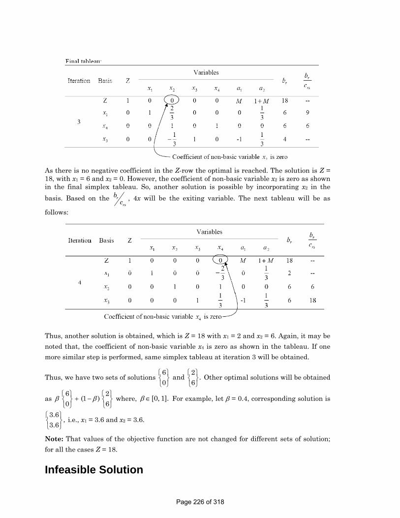
As there is no negative coefficient in the Z-row the optimal is reached. The solution is Z = 18, with x1 = 6 and x2 = 0. However, the coefficient of non-basic variable x2 is zero as shown in the final simplex tableau. So, another solution is possible by incorporating x2 in the basis. Based on the r
rs
bc , 4x will be the exiting variable. The next tableau will be as
follows:
Thus, another solution is obtained, which is Z = 18 with x1 = 2 and x2 = 6. Again, it may be noted that, the coefficient of non-basic variable x4 is zero as shown in the tableau. If one more similar step is performed, same simplex tableau at iteration 3 will be obtained.
Thus, we have two sets of solutions 6 2 and .0 6⎧ ⎫ ⎧ ⎫⎨ ⎬ ⎨ ⎬⎩ ⎭ ⎩ ⎭
Other optimal solutions will be obtained
as 6 2(1 )0 6
β β⎧ ⎫ ⎧ ⎫
+ −⎨ ⎬ ⎨ ⎬⎩ ⎭ ⎩ ⎭
where, [0, 1].β ∈ For example, let β = 0.4, corresponding solution is
3.6 ,3.6⎧ ⎫⎨ ⎬⎩ ⎭
i.e., x1 = 3.6 and x2 = 3.6.
Note: That values of the objective function are not changed for different sets of solution; for all the cases Z = 18.
Infeasible Solution
Page 226 of 318

Simplex Method S K Mondal Chapter 13
If in the final tableau, at least one of the artificial variables still exists in the basis, the solution is indefinite.
Reader may check this situation both graphically and in the context of Simplex method by considering following problem:
Maximize 1 23 2Z x x= +
Subject to 1 2 2x x+ ≤
1 2
1 2
3 2 18, 0
x xx x
+ ≥
≥
Minimization Versus Maximization Problems As discussed earlier, standard form of LP problems consist of a maximizing objective function. Simplex method is described based on the standard form of LP problems, i.e., objective function is of maximization type. However, if the objective function is of minimization type, simplex method may still be applied with a small modification. The required modification can be done in either of following two ways:
1. The objective function is multiplied by –1 so as to keep the problem identical and ‘minimization’ problem becomes ‘maximization’. This is because of the fact that minimizing a function is equivalent to the maximization of its negative.
2. While selecting the entering non-basic variable, the variable having the maximum coefficient among all the cost coefficients is to be entered. In such cases, optimal solution would be determined from the tableau having all the cost coefficients as non- positive (≤ 0).
Still one difficulty remains in the minimization problem. Generally the minimization problems consist of constraints with ‘greater-than-equal-to’ (≥) sign. For example, minimize the price (to compete in the market); however, the profit should cross a minimum threshold. Whenever the goal is to minimize some objective, lower bounded requirements play the leading role.
Constraints with ‘greater-than-equal-to’ (≥) sign are obvious in practical situations.
To deal with the constraints with ‘greater-than-equal-to’ (≥) and = sign, Big-M method is to be followed as explained earlier.
Page 227 of 318

Simplex Method S K Mondal Chapter 13
OBJECTIVE QUESTIONS (GATE, IES, IAS)
Previous 20-Years GATE Questions GATE-1. Simplex method of solving linear programming problem uses (a) All the points in the feasible region [GATE-2010] (b) Only the comer points of the feasible region (c) Intermediate points within the infeasible region (d) Only the interior points in the feasible region Common data for Question Q2 and Q3 [GATE-2008] Consider the Linear Programme (LP) Maximize 4x + 6y subject to 3x + 2y ≤ 6 2x + 3y ≤ 6 x, y ≥ 0
GATE-2. After introducing slack variables s and t, the initial basic feasible solution is represented by the tableau below (basic variables are s = 6 and t = 6, and the objective function value is 0).
–4 –6 0 0 0 s 3 2 1 0 6 t 2 3 0 1 6 x y s T RHS
After some simplex iteration, the following tableau is obtained
0 0 0 2 12 s 5/3 0 1 –1/3 2 y 2/3 1 0 1/3 2 x y s T RHS
From this, one can conclude that (a) The LP has a unique optimal solution (b) The LP has an optimal solution that is not unique (c) The LP is infeasible (d) The LP is unbounded GATE-3. The dual for the LP in Q 2 is: (a) Min 6u + 6v subject to 3u + 2v ≥ 4; 2u + 3v ≥ 6 u; and v ≥ 0 (b) Max 6u + 6u subject to 3u + 2v ≤ 4; 2u + 3v ≤ 6; and u, v ≥ 0 (c) Max 4u + 6v subject to 3u + 2v ≥ 6; 2u + 3v ≥ 6; and u, v ≥ 0 (d) Min 4u + 6u subject to 3u + 2v ≤ 6; 2u + 3v ≤ 6; and u, v ≥ 0
Page 228 of 318

Simplex Method S K Mondal Chapter 13
Previous 20-Years IES Questions IES-1. Which one of the following is true in case of simplex method of
linear programming? [IES-2009] (a) The constants of constraints equation may be positive or negative (b) Inequalities are not converted into equations (c) It cannot be used for two-variable problems (d) The simplex algorithm is an iterative procedure IES-2. Which one of the following subroutines does a computer
implementation of the simplex routine require? [IES 2007] (a) Finding a root of a polynomial (b) Solving a system of linear equations (c) Finding the determinant of a matrix (d) Finding the eigenvalue of a matrix IES-3. A tie for leaving variables in simplex procedure implies: [IES-2005] (a) Optimality (b) Cycling (c) No solution (d) Degeneracy IES-4. In the solution of linear programming problems by Simplex method,
for deciding the leaving variable [IES-2003] (a) The maximum negative coefficient in the objective function row is
selected (b) The minimum positive ratio of the right-hand side to the first decision
variable is selected (c) The maximum positive ratio of the right-hand side to the coefficients in
the key column is selected (d) The minimum positive ratio of the right-hand side to the coefficient in
the key column is selected IES-5. Match List-I (Persons with whom the models are associated) with
List-II (Models) and select the correct answer: [IES-2002] List-I List-II A. J. Von Newmann 1. Waiting lines B. G. Dantzig 2. Simulation C. A.K. Erlang 3. Dynamic programming D. Richard Bellman 4. Competitive strategies 5. Allocation by simplex method Codes: A B C D A B C D (a) 2 1 5 4 (b) 4 5 1 3 (c) 2 5 1 4 (d) 4 1 5 3 IES-6. Consider the following statements regarding linear programming:
1. Dual of a dual is the primal. [IES-2001] 2. When two minimum ratios of the right-hand side to the
coefficient in the key column are equal, degeneracy may take place.
3. When an artificial variable leaves the basis, its column can be deleted from the subsequent Simplex tables.
Select the correct answer from the codes given below:
Page 229 of 318

Simplex Method S K Mondal Chapter 13
Codes: (a) 1, 2 and 3 (b) 1 and 2 (c) 2 and 3 (d) 1 and 3 IES-7. In the solution of a linear programming problem by Simplex
method, if during iteration, all ratios of right-hand side bi to the coefficients of entering variable a are found to be negative, it implies that the problem has [IES-1999]
(a) Infinite number of solutions (b) Infeasible solution (c) Degeneracy (d) Unbound solution IES-8. A simplex table for a linear programming problem is given below:
5 X1
2 X2
3 X3
0 X4
0 X5
0 X6 Z
X4 1 2 2 1 0 0 8 X5 3 4 1 0 1 0 7 X6 2 3 4 0 0 1 10
Which one of the following correctly indicates the combination of entering and leaving variables? [IES-1994]
(a) X1 and X4 (b) X2 and X6 (c) X2 and X5 (d) X3 and X4 IES-9. While solving a linear programming problem by simplex method, if
all ratios of the right-hand side (bi) to the coefficient, in the key row (aij) become negative, then the problem has which of the following types of solution? [IES-2009]
(a) An unbound solution (b) Multiple solutions (c) A unique solution (d) No solution
Big-M Method IES-10. Consider the following statements: [IES-2000]
1. A linear programming problem with three variables and two constraints can he solved by graphical method.
2. For solutions of a linear programming problem with mixed constraints. Big-M-method can be employed.
3. In the solution process of a linear programming problem using Big-M-method, when an artificial variable leaves the basis, the column of the artificial variable can be removed from all subsequent tables.
Which one these statements are correct? (a) 1, 2 and 3 (b) 1 and 2 (c) 1 and 3 (d) 2 and 3 IES-11. A linear programming problem with mixed constraints (some
constraints of ≤ type and some of ≥ type) can be solved by which of the following methods? [IES-2009]
(a) Big-M method (b) Hungarian method (c) Branch and bound technique (d) Least cost method IES-12. When solving the problem by Big-M method, if the objective
functions row (evaluation row) shows optimality but one or more artificial variables are still in the basis, what type of solution does it show? [IES-2009]
(a) Optimal solution (b) Pseudooptimal solution
Page 230 of 318

Simplex Method S K Mondal Chapter 13
(c) Degenerate solution (d) Infeasible solution IES-13. Which one of the following statements is not correct? [IES-2008] (a) A linear programming problem with 2 variables and 3 constraints can be
solved by Graphical Method. (b) In Big-M method if the artificial variable can not be driven out it depicts
an optimal solution. (c) Dual of a dual is the primal problem. (d) For mixed constraints either Big-M method or two phase method can be
employed.
Page 231 of 318

Simplex Method S K Mondal Chapter 13
Answers with Explanation (Objective)
Previous 20-Years GATE Answers GATE-1. Ans. (b) Simplex method of solving linear programming problem uses only the
corner points of the feasible region. GATE-2. Ans. (b) As Cj = 0, 0 for x and y respectively therefore It is an optimal solution
but not unique. GATE-3. Ans. (a) Duplex method: Step-I: Convert the problem to maximization form so Choice may be (b) or (c).
Step-II: Convert (≥) type constraints if any to (≤) type by multiplying such constraints by (–1) so our choice is (b).
Previous 20-Years IES Answers IES-1. Ans. (d) IES-2. Ans. (b) IES-3. Ans. (d) IES-4. Ans. (b) IES-5. Ans. (b) IES-6. Ans. (a) IES-7. Ans. (d) IES-8. Ans. (a) The combination of entering and leaving variables corresponds to Z being
minimum and maximum value of row in table. IES-9. Ans. (a) While solving a linear programming problem by simplex method, if all the
ratios of the right hand side (bi) to the coefficient in the key row (aij) become negative, it means problem is having unbounded solution.
IES-10. Ans. (d) IES-11. Ans. (a) A linear programming problem with mixed constraints (some constraints
of ≤ type and some of ≥ type) can be solved by Big M-method which involves. (i) Objective function should be changed to maximization function. (ii) If the constraint is ≥ type, along with a slack variable an artificial
variable is also used. IES-12. Ans. (d) When solving the problem by Big-M method if the objective functions row
(evaluation row) shows optimality but one or more artificial variables are still in the basis, this shows infeasible solution.
IES-13. Ans. (b)
Page 232 of 318

14. Transportation Model
Theory at a Glance (For IES, GATE, PSU) Transportation problem: This is a special class of L.P.P. in which the objective is to transport a single commodity from various origins to different destinations at a minimum cost. The problem can be solved by simplex method. But the number of variables being large, there will be too many calculations. Formulation of Transportation problem: There are m plant locations (origins) and n distribution centres (destinations). The production capacity of the ith plant is ai and the number of units required at the jth destination bj. The Transportation cost of one unit from the ith plant to the jth destination cij.Our objective is to determine the number of units to be transported from the ith plant to jth destination so that the total transportation cost is minimum.
Let xij be the number of units shipped from ith plant to jth destination, then the general transportation problem is:
( )( )
1 1
1 2
1 2
Subjected tofor origin 1, 2, ......,
for origin 1, 2, ......,0
m n
ij iji j
thi i in i
thj j mj j
ij
C x
x x x a i i m
x x x b j i n
x
= =
+ + − − − + = =
+ + − − − + = =
≥
Σ Σ
The two sets of constraints will be consistent if 1 1
,m n
i ji j
a b= =
=Σ Σ which is the condition for a
transportation problem to have a feasible solution? Problems satisfying this condition are called balanced transportation problem.
Degenerate or non-Degenerate: A feasible solution to a transportation problem is said to be a basic feasible solution if it contains at the most (m + n – 1) strictly positive allocations, otherwise the solution will ‘degenerate’. If the total number of positive (non-zero) allocations is exactly (m + n – 1), then the basic feasible solution is said to be non-degenerate, if ‘(m + n – 1)’ → no. of allocated cell. Then put an ε →0 at a location so that all ui, vj can be solved and after optimality check put 0.ε =
Optimal solution: The feasible solution which minimizes the transportation cost is called an optimal solution.
Working Procedure for transportation problems: Step-1: Construct transportation table: if the supply and demand are equal, the problem
is balanced. If supply and demand is not same then add dummy cell to balance it.
Step-2: Find the initial basic feasible solution. For this use Vogel’s approximation Method (VAM). The VAM takes into account not only the least cost cij but also the costs that just exceed the least cost cij and therefore yields a better initial
Page 233 of 318

Transportation Model S K Mondal Chapter 14
solution than obtained from other methods. As such we shall confine our selves to VAM only which consists of the following steps:
Steps in VAM solution: 1. Determine the difference between the two lowest distribution costs for each row and
each column. 2. Select the row or column with the greatest difference. If greatest difference not
unique, make an arbitrary choice. 3. Assign the largest possible allocations within the restrictions to the lowest cost
square in the row and column selected. 4. Omit any row or column that has been completely satisfied by the assignment just
made. 5. Reallocate the differences as in step1, except for rows and columns that have been
omitted. 6. Repeat steps 2 to 5, until all assignment have been made.
Step-3: Apply Optimality Check In the above solution, the number of allocations must be ‘m+n-1’ otherwise the
basic solution degenerates. Now to test optimality, we apply the Modified Distribution (MODI) Method and examine each unoccupied cell to determine whether making an allocation in it reduces the total transportations cost and then repeat this procedure until lowest possible transportation cost is obtained. This method consists of the following steps:
1. Note the numbers ui along the left and vj along the top of the cost matrix such that their sums equals to original costs of occupied cells i.e. solve the equations [ ui+vj=cij] starting initially with some ui=0 (For allocated cell) (u or v –ive )
2. Compute the net evaluations wij=ui+vj-cij for all the empty cells and enter them in upper right hand corners of the corresponding cells.
3. Examine the sign of each wij. If all ijw 0,≤ then the current basic feasible solution is optimal. If even one ijw 0,> this solution is not optimal and we proceed further.
Step-4: Iterate towards optimal solution:
1. Choose the unoccupied cell with the largest wij and mark θ in it. 2. Draw a closed path consisting of horizontal and vertical lines beginning and
ending at θ -cell and having its other corners at the allocated cells. 3. Add and subtract θ alternately to an from the transition cells of the loop
subjected to rim requirements. Assign a maximum value to θ so that one basic variable becomes zero and the other basic variables remain non-negative. Now the basic cell whose allocation has been reduced to zero leaves the basis.
Step-5: Return to step 3 and repeat the process until an optimal basic feasible solution is obtained.
Example: 1
Page 234 of 318

Transportation Model S K Mondal Chapter 14
Solution:
Step-1: Above it is a balanced type transportation problem Step-2: VAM
A B C DSD
11
13
19
I
II
III
21 16 1325
17 18 14 23
32 41 18 41
6 10 12 15 4343
Availability
Destination
Source
Requirement
Page 235 of 318

S
St
To
All∴
Fov2,
At∴ AnAn bu
Hebu the
S K Mo
ep-3: App As
Sin ∴
o removem + n - 1
located cell Required
or that put , v3, v4, v5, vt first assum
u3 + v1 = nd u4 + v1 = nd u3 + v3 =
u1 + v3 = u4 + v4 = u4 + v5 =
ut u2 + v2 = u2 + v6 =
ere the probut allocated
u2 + v3 = u2 = 7 – 9
en v2 = 3 + 2
ondal
ply optimali number of a
nce all the n6optT =
e degener1 = 4 + 6 – 1 = 8 degenerd one ε but u1, u2, u3, u
v6. me u3=0 6 or v 6 or 9 or 9 or 2 or 2 or 3 5
blem so put cell column 7 9 = –2 2 = 5
Tr
ity check allocation =
net evaluatio6 17 3 18× + ×
racy 1 = 9 racy where? u4, and v1,
v1 = 6 u4 = 0 v3 = 9 u1 = 0 v4 = 2 v5 = 2
one ε so than (3) has m
14
ransport
= m + n – 1
on is (–ive) t8 7 27 1+ × +
at u2 is founaximum cos
4
tation M
i.e. ‘6’, we
then curren2 18 11× + ×
nd out for thst is ‘9’ so w
Model
e can apply M
nt solution is13 4 23+ × =
hat we can pwe will put
Chap
MODI meth
s optimal so796=
put ε on any ε on cell (2
pter 14
hod
olution
y of ‘*’ cell 2 – 3) i.e.,
Page 236 of 318

S K
v
Then ExamoptimStep-
m
Alloca
∴ W1. L
a
U
2. E R
Step-
A. F(a) N
(i) lta
(ii) Deacrvbvct
Put θ
K Monv6 = 5 + 2 = check optim
mple: 2 Inmality. -3: Optimm + n – 1 = ated cell = 6We can checLet u1 = allocated ce----
Using [ ui +
Empty cellRow-colum
2 – 1 2 – 2 3 – 2 1 – 3 2 – 3 1 – 4
Since the ne
-4: IteratFirst iteraNext basic f
Chose the ulower originthese cell (2and note θ
Draw a clending at θalternately cells of threquiremenvalue to θ becomes zevariables rcell whose ato zero leavsecond basi
θ =1 so that o
ndal 7
mality of the
n the next
mality check 3 + 4 – 1 =
6 ck optimalit0 then a
ell find out
+ vj = cij]
l mn
et evaluatio
tion towardtion feasible solu
unoccupied nal cost. In 2, 3) has low in it.
losed path θ -cell. Add to and fromhe loop su
nt s. Assig so that onero and t
remain 0≥ . allocation hves the basic solution (T
one cell can
Tran
e above prob
table the
6
ty according to u2, u3 ---- v
Calcwij = u– 5 + 2– 5 + 33 + 3 –0 + 12
– 5 + 10 + 6
ons in two ce
ds optimal
ution
cell with th Table 1, ce
wer original
beginning and subtram the transubject the gn a maxine basic varthe other
Now the has been reds. This giveTable 2).
n empty
nsportat
blem.
ere is some
o all v1, v2,
ulation ui + vj – cij 2 – 1 = – 4 3 – 0 = – 2 – 8 = 0 – 2 2 – 11 = 1 2 – 11 = 1 – 7 = –1 ells are posi
l solution.
he maximumells (1 – 3) l cost 6, the
and actθ , sition rim imum riable basic basic
duced es the
tion Mod
e allocated
itive a bette
m wij. In cas and (2, 3) refore we ta
del
d cell and
Improve
No No No Yes Yes No
er solution c
se of a tie, seach have
ake this as
Chapte
d we only
ement
can be found
select the onwij = 1 andthe next ba
er 14
check
d
ne with d out of asic cell
Page 237 of 318

Transportation Model S K Mondal Chapter 14
Here total transportation cost Rs. 1 2 5 3 1 6 6 5 2 15 2 9 100= × + × + × + × + × + × ×⎡ ⎤⎣ ⎦ Rs. 10,100= B. Optimality check
Empty cell Calculation Improvement ij i j ijW U V C⎡ ⎤= + −⎣ ⎦ 2 – 1 – 6 + 2 – 1 = – 5 No 2 – 2 – 6 + 3 – 0 = – 3 No 3 – 2 3 + 3 – 8 = – 2 No 1 – 3 0 + 12 – 11 = 1 Yes 1 – 4 0 + 6 – 7 = – 1 No 2 – 4 – 6 + 6 – 1 = – 1 No Second Iteration (a) Next basic feasible solution:
Put θ = 1 (b) Optimality Check
V =21 V =32 V =123 V =64
U =01
U =-62
U =33
-Q +Q
+Q -Q
Page 238 of 318

Transportation Model S K Mondal Chapter 14
Empty cell Calculation Improvement ij i j ijW U V C⎡ ⎤= + −⎣ ⎦ 1 – 1 0 + 1 – 2 = – 1 No 2 – 1 – 5 + 3 – 1 = – 5 No 2 – 2 – 5 + 3 – 0 = – 2 No 3 – 2 4 + 3 – 8 = – 1 No 1 – 4 0 + 5 – 7 = – 2 No 2 – 4 – 5 + 5 – 1 = – 1 No So this basic feasible solution is optimal
Optimal Transportation cost Rs. 5 3 1 11 1 6 7 5 1 15 2 9 100= × + × + × + × + × + × ×⎡ ⎤⎣ ⎦ Rs. 10,000 /= −
V =11 V =32 V =113 V =54
U=01
(7)
U =-92
U =43
Page 239 of 318

S
O
GA
GA
GA
GA
S K Mo
OBJEC
PATE-1.
ATE-2.
ATE-3.
ATE-4.
ondal
CTIVE
PreviouFor the stand n deoptimal soxij values upper bou(a) mn
A compansupplies fD1 requirWarehousit can takproblem isupply po(or totalrespective(a) 2, 4, 90
The supplthe demasolving th(a) A dumm(b) A dumm(c) No solu(d) None so
A firm is (P, Q, anditems (in are givenpolicy reqsupplied supplier minimumprocurem(a) 350
Tr
QUES
us 20-Ytandard trestinationsolution (lo(amounts
und for thi(b) 2(m
ny has two from S1 anres a minise D2 requke as muchis to be foroints, the nl demandely are: (
ly at threeand at the his transpomy source omy destinatution exists olution exis
required td R). The p
Rs.) by sun in tablquires thaby only osupply o
m total ment to the
(b)
ransport
STIONS
Years ransportats and totaowest cost)from sourcis number + n)
factories Snd S2 are 5imum of 2
uires a minh as can brmulated fnumber of
d) in the
(b) 2, 4, 110
e sources is four dest
ortation prf capacity 4
tion of capacas the probts as the pr
to procure prices quotuppliers S1le. The m
at each itemone supplionly one
cost (in firm is: ) 360
tation M
S (GA
GATEtion linearal supply ) with the ce i to dest is:
(c) m + n
S1, S2 and0 and 40 u20 units animum of 2be suppliedfor the abof demand e balance
(c
s 50, 40 andtinations iroblem 40 units is ncity 40 unitslem is infea
roblem is de
three itemted for the1, S2 and Smanagemem has to bier and on
item. Thn Rs.)
(c)
Model
ATE, I
E Quesr programm
equaling smallest ntinationj) i
d two wareunits respeand a max20 units and. A balanove situatipoints, an
ed transp
c) 3, 4, 90
d 60 units s 20, 30, 1
needed s is needed
asible generate
ms se S3 nt be ne he of
) 385
Chap
IES, IA
tions me with mtotal dem
number of is desired.
[GA(d) m + n –
ehouses D1ectively. Waximum of nd, over anced transpion. The nund the totaportation
[GA (d)
respective10 and 50
[GA
[GAT
(d)
pter 14
AS)
m sources mand, an non-zero The best
ATE-2008] – 1
1, D2. The arehouse 40 units.
nd above, portation umber of al supply
problem ATE-2005]
3, 4, 110
ely whilst units. In
ATE-2002]
TE-2006]
395
Page 240 of 318

Transportation Model S K Mondal Chapter 14
Previous 20-Years IES Questions IES-1. Consider the following statements: [IES-2007] The assignment problem is seen to be the special case of the
transportation problem in which 1. m = n 2. All ai = 1 3. xij = 1
(The symbols have usual meaning)
Which of the statements given above are correct? (a) 1, 2 and 3 (b) 1 and 2 only (c) 2 and 3 only (d) 1 and 3 only IES-2. In order for a transportation matrix which has six rows and four
columns, not to be degenerate, how much must be the number of allocated cells in the matrix? [IES-2007]
(a) 6 (b) 9 (c) 15 (d) 24 IES-3. Which one of the following is not the solution method of
transportation problems? [IES-2006] (a) Hungarian method (b) Northwest corner method (c) Least cost method (d) Vogel's approximation method IES-4. Which one of the following conditions should be satisfied for the
application of optimality test on an initial solution of transportation model? [IES-2004]
(a) Number of allocations should be less than m + n – 1 (b) Number of allocations should be equal to m + n – 1 (c) Number of allocations should be equal to m + n (d) Number of allocations should be more than m + n IES-5. In a connected network of 'n' arcs (roads) joining 'm' vertices
(towns), a selection of roads is taken up for resurfacing based on a minimum spanning tree of network as being the least cost solution. This spanning tree will contain [IES-1994]
(a) m arcs (b) (m + 1) arcs (c) (m – 1) arcs (d) (m + n – 1) arcs IES-6. Consider the following statements on transportation problem:
1. In Vogel's approximation method, priority allotment is made in the cell with lowest cost in the column or row with least penalty
2. The North-West corner method ensures faster optimal solution 3. If the total demand is higher than the supply, transportation
problem cannot be solved 4. A feasible solution may not be an optimal solution.
Which of these statements are correct? [IES-2003] (a) 1 and 4 (b) 1 and 3 (c) 2 and 3 (d) 2 and 4 IES-7. Assertion (A): In the solution of transportation problem, for
application of optimality test, the number of allocations required is m + n – 1 and these should be in independent positions. [IES-2003]
Reason (R): If the number of allocations is not m + n – 1, values of all oddments, i.e., ui and vj cannot be found.
(a) Both A and R are individually true and R is the correct explanation of A
Page 241 of 318

Transportation Model S K Mondal Chapter 14
(b) Both A and R are individually true but R is not the correct explanation of A
(c) A is true but R is false (d) A is false but R is true IES-8. Assertion (A): Vogel's approximation method yields the best initial
basic feasible solution of a transportation problem. [IES-2000] Reason (R): Vogel's method gives allocations to the lowest cost
elements of the whole matrix. (a) Both A and R are individually true and R is the correct explanation of A (b) Both A and R are individually true but R is not the correct explanation
of A (c) A is true but R is false (d) A is false but R is true IES-9. In a transportation problem North-West corner rule would yield (a) An optimum solution (b) An initial feasible solution [IES-1999] (c) A Vogel's approximate solution (d) A minimum cost solution IES-10. In a transportation problem, the materials are transported from 3
plants to 5 warehouses. The basis feasible solution must contain exactly, which one of the following allocated cells? [IES-1998]
(a) 3 (b) 5 (c) 7 (d) 8 IES-11. When there are 'm' rows and 'n' columns in a transportation
problem, degeneracy is said to occur when the number of allocations is: [IES-1997]
(a) Less than (m + n – 1) (b) Greater than (m + n – 1) (c) Equal to (m – n – 1) (d) Less than (m – n – 1) IES-12. In order for a transportation matrix which has six rows and four
columns not to degenerate, what is the number of occupied cells in the matrix? [IES-2008]
(a) 6 (b) 9 (c) 15 (d) 24 IES-13. Assertion (A): Transportation problem can be solved by VAM
heuristic much faster as compared to the solution through linear programming method. [IES-1996]
Reason (R): VAM heuristic gives an approximate solution. It is checked for optimality test. If it is optimal, the algorithm stops there. If it is not an optimal solution, then improved solutions are found out through very little iteration till optimality is reached.
(a) Both A and R are individually true and R is the correct explanation of A (b) Both A and R are individually true but R is not the correct explanation
of A (c) A is true but R is false (d) A is false but R is true IES-14. A solution is not a basic feasible solution in a transportation
problem if after allocations. [IES-1996] (a) There is no closed loop (b) There is a closed loop
Page 242 of 318

Transportation Model S K Mondal Chapter 14
(c) Total number of allocations is one less than the sum of numbers of sources and destinations
(d) There is degeneracy IES-15. Match List-I (O.R. Techniques) with List-II (Application) and select
the correct answer using the codes given below the lists: [IES-1995] List-I List-II A. Linear programming 1. Warehouse location decision B. Transportation 2. Machine allocation decision C. Assignment 3. Product mix decision D. Queuing theory 4. Project management decision 5. Number of servers decision Codes: A B C D A B C D (a) 1 2 3 5 (b) 3 1 2 5 (c) 1 3 4 5 (d) 3 2 1 4 IES-16. The solution in a transportation model (of dimension m × n) is said
to be degenerate if it has [IES-1995] (a) Exactly (m + n – 1) allocations (b) Fewer than (m + n – 1) allocations (c) More than (m + n – 1) allocations (d) (m × n) allocations IES-17. Assertion (A): In distribution problem, unit cost of production as
well as transportation cost is considered. [IES-1994] Reason (R): The Vogel approximation method can reduce the
number of iterations required to move from the initial assignment to the optimal solution.
(a) Both A and R are individually true and R is the correct explanation of A (b) Both A and R are individually true but R is not the correct explanation
of A (c) A is true but R is false (d) A is false but R is true IES-18. Consider the following statements: [IES-1993] In a transportation problem, North-West corner method would yield 1. An optimum solution 2. An initial feasible solution 3. Vogel's approximate solution Of these statements: (a) I alone is correct (b) 2 alone is correct (c) 3 alone is correct (d) 2 and 3 are correct IES-19. In a 6 × 6 transportation problem, degeneracy would arise, if the
number of filled slots were: [IES-1993] (a) Equal to thirty six (b) More than twelve (c) Equal to twelve (d) Less than eleven
Previous 20-Years IAS Questions IAS-1. Consider the location of a warehouse to distribute books for the
cities of Bombay, Bangalore and Calcutta. The estimated volume of distribution to Bombay, Bangalore and Calcutta are 55,000, 20,000
Page 243 of 318

Transportation Model S K Mondal Chapter 14
and 25,000 units respectively. Using some appropriate origin, the (x, y) co-ordinates of Bombay, Bangalore and Calcutta can be approximated as (10, 20), (20, 10) and (30, 30) respectively. The (x, y) co-ordinates or the optimal location would be: [IAS-1998]
(a) (20, 20) (b) (l0, 20) (c) (30, 20) (d) (20, 30)
Page 244 of 318
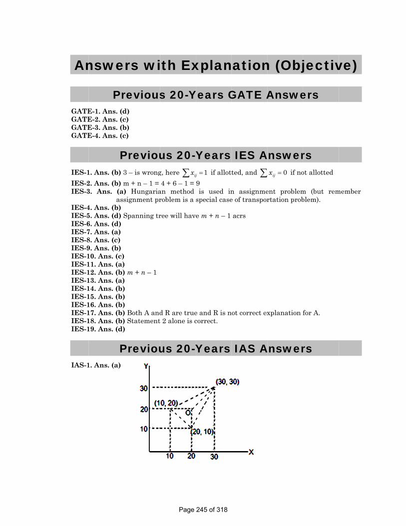
S K
An
GATEGATEGATEGATE
IES-1IES-2IES-3
IES-4IES-5IES-6IES-7IES-8IES-9IES-1IES-1IES-1IES-1IES-1IES-1IES-1IES-1IES-1IES-1
IAS-1
K Mon
nswe
PrE-1. Ans. (dE-2. Ans. (cE-3. Ans. (bE-4. Ans. (c
P1. Ans. (b) 32. Ans. (b) m3. Ans. (a)
ass4. Ans. (b) 5. Ans. (d) S6. Ans. (d) 7. Ans. (a) 8. Ans. (c) 9. Ans. (b) 10. Ans. (c)11. Ans. (a)12. Ans. (b)13. Ans. (a)14. Ans. (b)15. Ans. (b)16. Ans. (b)17. Ans. (b)18. Ans. (b)19. Ans. (d)
P1. Ans. (a)
ndal
rs wi
reviousd) c) b) c)
Previou3 – is wrongm + n – 1 = ) Hungariasignment pr
Spanning tr
) ) m + n – 1 ) ) ) ) ) Both A and) Statement)
Previou
Tran
ith Ex
s 20-Y
us 20-Yg, here ijx∑ 4 + 6 – 1 = an method roblem is a
ree will hav
d R are truet 2 alone is c
us 20-Y
nsportat
xplan
Years G
Years 1j = if allott
9 is used in
special case
e m + n – 1
e and R is ncorrect.
Years
tion Mod
nation
GATE A
IES Ated, and ∑
n assignmee of transpor
acrs
ot correct ex
IAS A
del
n (Obj
Answe
Answer0ijx = if no
ent problemrtation prob
xplanation f
Answer
Chapte
jectiv
ers
rs ot allotted
m (but remblem).
for A.
rs
er 14
ve)
member
Page 245 of 318

Transportation Model S K Mondal Chapter 14
Conventional Questions with Answer Conventional Question [ESE-2000] A company has three plants at A, B, C which supply to warehouses located at D, E, F, G and H. Weekly plant capacities are 200,125 and 225 tons respectively. Weekly warehouses requirements are 75, 105, 130, 155 and 85 tons respectively. Unit transportation cost matrix is given below:
Determine the optimum cost distribution pattern and also the minimum total cost.
Solution: Step-1:
It is a balanced type transportation problem. Step-2: VAM
Step-3: m + n – 1 = 3 + 5 – 1 = 7 And number of allocated cell = 7 ∴ It is not degenerate so we can check optimality.
ToFR
A
B
C
D E F G H
50
45
80
82
70
45
70 65
65
75 60
60 35
50
40
ToFR
A
B
C
D E F G H
50
45
80
82
70
45
70 65
65
75 60
60 35
50
40
200
125
225
75 105 130 155 85550
550
Page 246 of 318

Transportation Model S K Mondal Chapter 14
Step-4: Modi Method First Iteration
Put Q = 85
Empty Cell Calculation Improvement ij i j ijW U V C⎡ ⎤= + −⎣ ⎦ 1 – 1 0 + 40 – 50 = – 10 No 1 – 2 0 + 45 – 82 = – 37 No 1 – 5 0 + 40 – 35 = 5 Yes 2 – 2 5 + 45 – 70 = – 20 No 2 – 4 5 + 60 – 65 = 0 No 2 – 5 5 + 40 – 50 = – 5 No 3 – 1 0 + 40 – 80 = – 40 No 3 – 3 0 + 65 – 75 = – 10 No Second Iteration
Empty Cell Calculation Improvement (Do yourself and will find no improvement)
So this basic feasible solution is optimal
Minimum cost: 75 45 105 45 80 65 50 70 35 60 120 60 85 35 Rs.29,075× + × + × + × + × + × + × = Conventional Question [UPSC-1998] In the state of Bihar, in a particular region there are 5 coalmines which produce the following output at the indicated production costs:
50
45
80
82
70
45
70 65
65
75 60
60 35
50
40
V =401 V =452V =653 V =604 V =405
U =01
U =52
U =03
(75)
(80)
(50)
(120)-Q
+Q
+Q -Q
(105) (35) (85)
50
45
80
82
70
45
70 65
65
75 60
60 35
50
40
V =401 V =952V =653 V =604 V =355
U =01
U =52
U =03
(75)
(80)
(50)
(105)
(-) (-)
(-)
(-)
(-)
(35)
(-)
(120) (-)
(-)
(85)
Page 247 of 318

Transportation Model S K Mondal Chapter 14
Before the coal can be sold to the steel making units, it must be cleaned and graded at one of the 3 coal preparation plants. The capacities and operating cost of the 3 plants areas follows.
All coal is transported by rail at a cost Rs. 50 per metric ton kilometre and the distance in kilometre from each mine in the preparation plants indicated below:
(i) Using a transportation model, determine how the output of each mine should be allocated to the three preparation plants to optimise cost.
(ii) Are alternative approaches possible? If so, what is the logic of 1st allocation in these alternatives?
(iii) What is degeneration and when can it happen? [20]
Solution: Using Transportation Model
Step-1: Cost matrix per metric tonne is given by [Rs.]
Here Demand > supply, hence add dummy source with infinite cost. Step-2: Using VAM allocate
MineOutputm.tons/day
Production Cost units of100 Rs. Per metric ton
1 120 252 150 293 80 344 160 265 140 28
PlantsCapacity metric
tons/dayOpterating cost units of100 Rs. Per metric ton
A 300 2B 200 3C 200 3
1 2 3 4 5A 22 44 26 52 24B 18 16 24 42 48C 44 32 16 16 22
Preparation Plants
Distance kilometres to Mines
Coal mines A B C Supply
12500+200+22*50
38002500+300+18*150
=37002500+300+44*50
=5000 120
22900+200+2200
53002900+300+16*50
=40002900+300+32*50
=4500 150
33400+200+1300
=49003900+300+24*50
=49003400+300+16*50
4500 80
42600+200+2600
=54002600+300+42+50
50002600+300+16*50
=3700 160
52800+200+1200
42002800+300+48+50
=55002800+300+22*50
4200 140Demand 300 200 200
Page 248 of 318
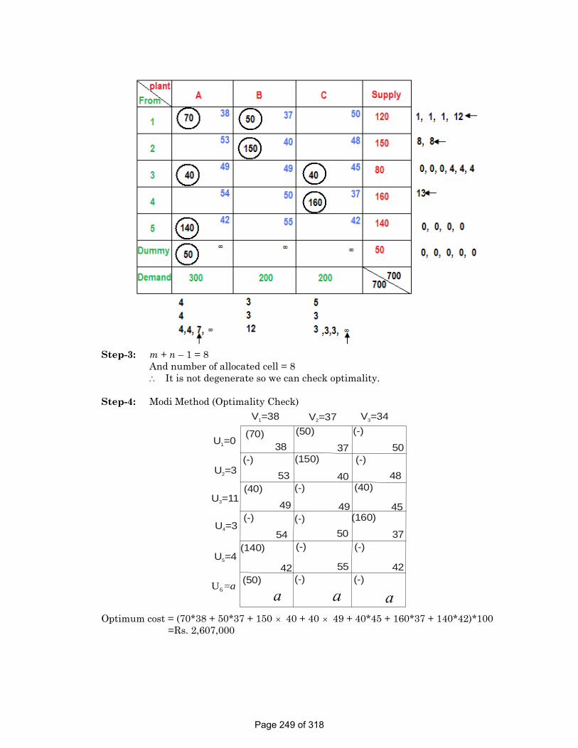
Transportation Model S K Mondal Chapter 14
Step-3: m + n – 1 = 8 And number of allocated cell = 8 ∴ It is not degenerate so we can check optimality. Step-4: Modi Method (Optimality Check)
Optimum cost = (70*38 + 50*37 + 150 × 40 + 40 × 49 + 40*45 + 160*37 + 140*42)*100 =Rs. 2,607,000
(70)38
(50)
37(-)
50(-)
53
(150)
40 48
U =01
U =32
U =113
U =34
U =45
6U =a
V =381 V =372 V =343
(-)
(40)
49 49
(-) (40)
45(-)
54
(-)
50
(160)
37(140)
42
(-)
55
(-)
42(50) (-)(-)
Page 249 of 318

15. Assignment Model
Theory at a Glance (For IES, GATE, PSU) An assignment problem is a special type of transportation problem in which the objective is to assign a number of origins to an equal number of destinations at a minimum cost (or maximum profit).
Formulation of an assignment problem: There are n new machines mi (I = 1, 2, ......, n) which are to be installed in a machine shop. There are n vacant spaces sj (j = 1, 2, ......, n) available. The cost of installing the machine mi at space Sj is Cij rupees.
Let us formulate the problem of assigning machines to spaces so as to minimize the overall cost.
Let xij be the assignment of machine mi to space sj i.e. Let xij be a variable such that
⎧
= ⎨⎩
1, if machine is installed at space 0, otherwise
th th
iji jx
Since one machine can only be installed at each place, we have xi1 + xi2 + ........ xin = 1 for mi (I = 1, 2, 3, ..., n) x1i + x2i + .... + xij =1 for sj (j = 1, 2, 3, ..., n)
Also the total installation cost is = =∑∑
1 1
n n
i j iji j
c x
Thus assignment problem can be stated as follows:
Determine xij ≥ 0 (j = 1, 2, 3, ....., n) so as to minimize(z) = = =∑∑
1 1
n n
i j iji j
c x
Subject to the constraints
= =
= = = =∑ ∑1 1
1, 1, 2, ....., and 1, 1, 2, 3, ....,n n
ij iji j
x j n x i n
This problem is explicitly represented by the following n × n cost matrix:
This assignment problem constitutes n! possible ways of installing n machines at n spaces. If we enumerate all these n! alternatives and evaluate the cost of each one of them and select the one with the minimum cost, the problem would be solved. But this method would
S1 S2 S3
Spaces
Sn
C31 C32 C33
Mn
Machines
C11 C12 C13
C21 C22 C23
M1
M2
M3
Cn1 Cn2 Cn3
Cnn
C1n
C2n
C3n
Page 251 of 318

Assignment Model S K Mondal Chapter 15
be very slow and time consuming, even for small value of n and hence it is not at all suitable. However, a much more efficient method of solving such problems in available this is the Hungarian method for solution of assignment problems which we describe below:
1. Given: Original Cost Matrix 2. Subtract the lowest entry of each column and get Job- opportunity matrix 3. Subtract the lowest entry from each row of Job- opportunity matrix and get total
opportunity cost matrix.
Example:
Original Cost Matrix
Subtract lowest entry of each column
Job-opportunity matrix
Subtract lowest entry of each row
Subtract lowest element of undotted matrix from all uncut element and add the same to corners of cut line element.
Iteration-2
Assign A is 4; B is 3; C is 2; D is 1; E is 5 VIMP: For maximization by assignment we have to firstly changed original cost matrix by putting (–ve) at all cost element.
A B C D E
1
2
3
4
5
32 38 40 28 40
40 24 28 21 36
41 27 33 30 37
22 38 41 36 36
29 33 40 35 39
It is a minimization problem
10
18
19
0
7
14
0
12 7 4
0 0 0
3 5 9 1
14 13 15 0
9 12 14 3
6-2 10-2 8-2 3-2
O
O
O O O
O
O
O
18
18-2 2-2 8-2
O 14 13 15
+Z
+Z
4-2 6-2 9-211=2
4-2
4 8 6-1 1-1 0
18+1 0+1
0
0 0 2+1
16
0
2
14
4
2-1 6-10
13-1
7-1 9-1
15-1 2
0
A B C D E
1
2
3
4
5
4 8 5 0 019 1 0 0
16 0 051
0
2 4
14 12
6
14 2
08
3
Page 252 of 318

Assignment Model S K Mondal Chapter 15
Example:
Maximize
Then first change all element (–ve), then original cost matrix is:
Minimize:
Subtract Column
Subtract Row
1
2
3
A B C
32 38 40
40 24 28
41 27 33
A B C
-32 -38 -40
-40 -24 -28
-41 -27 -33
9
1
0
0
14
11
0
12
7
9
1
0
0
13
11
0
11
7
6
16 0 0
0 5
50 0
CA B
A-2
B-1
C-3
Page 253 of 318

Assignment Model S K Mondal Chapter 15
OBJECTIVE QUESTIONS (GATE, IES, IAS)
Previous 20-Years IES Questions IES-1. Consider the following statements in respect of assignment method
of optimization: [IES-2006] 1. The matrix format of the method must be a square matrix. 2. Some type of rating has to be given to the performance of each
pairing. Which of the statements given above is/are correct? (a) Only 1 (b) Only 2 (c) Both 1 and 2 (d) Neither 1 nor 2 IES-2. In an assignment problem having n facilities and n jobs, what is the
number of possible ways of making assignments? [IES-2005] (a) nl (b) n2 (c) 2n (d) 2n IES-3. The assignment algorithm is applicable to which of the following
combined situations for the purpose of improving productivity? 1. Identification of sales force-market [IES-1998] 2. Scheduling of operator-machine 3. Fixing machine-location. Select the correct answer using the codes given below: Codes: (a) 1, 2 and 3 (b) 1 and 3 (c) 2 and 3 (d) 1 and 2
Answers with Explanation (Objective)
Previous 20-Years IES Answers IES-1. Ans. (a) There is nothing about performance.
IES-2. Ans. (a)
IES-3. Ans. (c)
Page 254 of 318

Assignment Model S K Mondal Chapter 15
Conventional Questions with Answer Conventional Question [ESE-2010] Question: Transportation costs from manufacturing plants to warehouses are given in table. They are in euros. Solve this problem to minimize the cost of transportation by stating the steps used in the algorithm. [15 Marks]
Warehouse PLANT A B C D
1 10 8 10 8 2 10 7 9 10 3 11 9 8 7 4 12 14 13 10
Answer: We have to use Hungarian method for this assignment problem. It is a special case of transportation problem. To minimize the cost of Transportation:
Warehouse PLANT A B C D
1 10 8 10 8 2 10 7 9 10 3 11 9 8 7 4 12 14 13 10
Step 1. Select minimum entry in column. Subtract from each element.
Warehouse A B C D
1. 0 1 2 1 2. 0 0 1 3 3. 1 2 0 0 4. 2 7 5 3
Step 2. Select minimum entry in each row and subtract it from each element and draw matrix and draw minimum no. of lines either horizontal and vertical covering all zeros.
B CA D
1
2
3
4 5
0
0
0
1
0
3
1
0
2
01 2
3
1
Warehouse
1
Step.3. The lines are less than number of rows and column. Therefore select minimum entry from rest element and subtract it from all non zero rows and column element and add same entry at the intersection points of lines.
Page 255 of 318

Assignment Model S K Mondal Chapter 15
B CA D
1
2
3
4 5
0
0
0
1
0
3 -1
1 -1
0
2 -1
0
1 -1
2+1
3 -1
1 -11+1
Warehouse
Repeat step 2
B CA D
1
2
3
4 5
Warehouse
0
0
0
2
1
0
3
1
0
0
2
0
0
2
0
No. of lines is equal is to no. of rows or columns hence solution is optimal Step for assignment – select rows and columns that has minimum of zeros
B CA D
1
2
3
4 5
0
0
0
2
1
0
3
1
0
0
2
0
0
2
0
Warehouse
Select: - Select that row or column that has minimum number of zero. Cost 2 - B 7 3 - C 8 1 - A 10 4 - D 10 Total cost = 35 euros Conventional Question [ESE-2009] Four technicians are required to do four different jobs. Estimates of time to
complete every job as provided by the technicians are as below:
Technician Hours to Complete Job Job 1 Job 2 Job 3 Job 4
A B C D
20 24 22 37
36 34 45 40
31 45 38 35
27 22 18 28
Assign the jobs to technicians to minimize the total work-time. State the steps taken in the algorithm used. [15-Marks]
Page 256 of 318

Assignment Model S K Mondal Chapter 15
Solution:. Step (1): Subtracting the minimum value in the row from each element in that row.
Step (2): From the resulting matrix, in each column, subtract the minimum value in the column from each element in that column.
0 16 11 17
2
12
23
4 27 20
79
0
0
0
12
Step (3): Checking whether a feasible assignment could be obtained by assigning
at the elements contain zeros.
0 174
9
16 0
0
0
0
4
4
2
13
00
15
0 17
2
4
9
16 0
0
0
0
4
4 13
00
15
Hence we find feasible solution, the optimum assignments is A → 1, B → 2, C → 4, D → 3 Total work time, T = 20 + 34 + 18 + 35 = 107
A
B
C
D
1 2 3 4
20 36 31 37
24 34 45 22
38 18
40 35
22 45
37 28
Page 257 of 318

Assignment Model S K Mondal Chapter 15
Conventional Question [ESE-2008] What are the differences between transportation and assignment problems, in
relation to (i) Structure of the problem; (ii) Procedure for solving? [ 2 Marks] Solution: The transportation problem is one of the sub-classes of L.P.Ps. in which the objective is
to transport various quantities of a single homogeneous commodity, that are initially stored at various origins, to different destinations in such a way that the total transportation cost is minimum. To achieve this objective we must know the amount and location of available supplies and the quantities demanded. In addition, we must know the costs that result from transporting one unit of commodity from various origins to various destinations.
(ii) An assignment problem is a particular case of transportation problem in which a number of operations are to be assigned to an equal number of operators, where each operator performs only one operation. The objective is to maximize overall profit or minimize overall cost for a given assignment schedule.
An assignment problem is a completely degenerate form of a transportation problem. The units available at each origin and units demanded at each destination are all equal to one. That means exactly one occupied cell in each row and each column of the transportation table i.e., only n occupied cells in place of the required n + n – 1 (= 2 n -1)
Page 258 of 318

1
QueA sim
Typicdelays
Key •
•
(i) f
•
♦
Table
S. No
1.
2.
3.
4. 5.
6.
16.
Theor
euing Tmple but typ
al measuress of custome
elementsCustomepeople, maServer: receptioni
Calling pofinite or infi
Finite pobeing servrepair arrInfinite pcustomerscustomers
e: Some Apo. Applic
Area Factory Assemb MachinmainteAirportBank Walk-in
Qu
ry at a
Theory pical queuin
s of system ers.
s of queuer: refers toachines, trurefers to
ist, repairpe
opulation: finite. opulation mved and wairival rate bepopulations being servs.
pplicationscation
y
bly line
ne enance t
n
ueuin
a Glanc
or Waitng model
performanc
uing systeo anything tucks, emails
any resouersons, retri
The popula
model: If iting, e.g., mecomes zero.n model: Ived and wait
s of WaitinArrival
Material/to Sub-assem Repair toolequipmentPlane Customer Job seeker
ng M
ce (Fo
ting Lin
ce are serve
ems that arrivess. urce that ieval machi
ation of pot
arrival ratemodel of one. If arrival rting, e.g., sy
ng Line ProWai
ools
mblies
ls & t
rs
In-p(WIPWIP MacrepaPlanDep App
odel
r IES,
ne
er utilization
s at a facili
provides tnes, runway
tential custo
e depends oe corporate j
rate is not ystems with
oblem iting Line
process invenP)
P
chines neediair nes ready toosit/withdra
licants
l
GATE
n, length of
ity and requ
he requestys at airpor
omers may
on the numjet, if it is b
affected bh large popu
Ser
ntory
ing
o fly awal
Wor EmcurrprocMai RunBancomInte
, PSU)
waiting line
uires servic
ted servicert.
be assumed
mber of cusbeing repair
by the numulation of po
rvice Facil
rk stations
ployees rently cessing the intenance cr
nway nk employed
mputer erviewers
)
es, and
ce, e.g.,
e, e.g.,
d to be
tomers red, the
mber of otential
ity
WIP rew
d &
Page 259 of 318

S
(ii
It govarr
Th
S K Mo
7. 8. 9.
10. 11.
12.
13.
14.
15. 16.
intePhoGovPostExeGro TrafcrosCarstatRail ToolHos
i) Arrival times, wprobabilFor a giv
(P xwhere: P(x 1/
can be shoverned by trivals is Poi
he correspon
( )P t λ=
ondal erview one exchangvt. office t office
ecutive note cery shop
ffic light ssing r service tion lways
l crib spital
Pattern awhich is the lity distribuven arrival r
)−
=ex
x) : Probabilx : Number λ : Average
/λ : Mean timwn mathemthe exponenisson distribnding expon
te λλ −
ge
Dialed Files LettersDictatioCustom Vehicle Cars Passeng MechanPatient
Waiting lat the Sys time betwetion. rate (λ), a d
λλ−
!
x
xity of x arriv arrivals pe arrival rateme betweenmatically thntial distribbution.
nential distr
Queui
number
on note
mers
es
gers
nics ts
CBMLCcV U WorWS
ine cost antem: The pen two cons
discrete Pois
For
val. er unit time.e.
n arrivals orhat the probbution when
ribution for
ng Mode
Caller Backlog filesMailbox Letters to beCustomer oncounter Vehicles in l
Unserviced c
Waiting pason platform/room Waiting mecSick people
nd service probability secutive arr
sson distribu
=r 0x
.
r inter-arrivbability distn the proba
inter-arriva
el
s
e typed n the
line
cars
sengers /waiting
chanics
SCPSCaT S T SDf
levels distribution
rivals, may a
ution is give
0, 1, 2,
al time. tribution of ability distr
al time is giv
Chap SwitchboardClerks Postal emplSecretary Checkout cland bag pacTraffic sign Service faci Trains Store keepeDoctor & opfacility
n of the intalso be gove
en by:
, 3, . . .
f inter-arrivribution of n
ven by:
pter 16
d
loyees
lerks ckers als
lities
er peration
ter-arrival erned by a
. . .
val time is number of
Page 260 of 318

S K
QueThe qnumb
Anothcustom F L S
For exreceiv
Ser
K Mon
eue Chqueue may bber. It may bher charactemers waitinFIFO : LIFO : SIRO : xample, in ave service pr
rvice Ch
ndal
Po
Expon
aracterbe considerebe unlimitederistic of a qng in queue First – In Last – In – Service – Ia railway rerior to other
haracte
Q
oisson distr
nential dis
risticsed to be limid or infinitequeue is its would recei– First – Ou– First – OuIn – Randomeservation cr customers
eristics
Queuing
ribution fo
stribution
ited when ite otherwise. discipline. Qive service. ut ut m – Order, eounter, the joining this
g Model
or arrival t
for service
ts length can Queue disciThese rules
etc. customer, ws queue late
time
e times
nnot exceed
pline is the s may be:
who enters fer. This is a
Chapte
d a certain
rule by whi
first in queu FIFO syste
er 16
ich
ue, will em.
Page 261 of 318

S
Seserserph
S K Moervice systervers, numbrvice mean
hases).
ondal m may varber of phass that once
Sing
ry dependinses, etc. A e an arrival
Single cha
gle channe
Multi cha
Multi Ch
Queui
ng upon thsingle chan
l enters the
annel, sing
el, multiph
annel, sing
annel, Mul
ng Mode
he number nnel servere service, it
gle phase s
hase (3-pha
gle phase s
ltiphase Sy
el
of service has one st is served
system
ase) system
ystem
ystem
Chapchannels, nerver. A that three st
m
pter 16 number of hree-phase tations (or
Page 262 of 318

Queuing Model S K Mondal Chapter 16
Single-Line-Single-Server Model Queuing models may be formulated on the basis of some fundamental assumptions related to following five features:
• Arrival process • Queue configuration • Queue discipline • Service discipline, and • Service facility.
Let us understand the M/M/1 model first. Following set of assumptions is needed: 1. Arrival Process: The arrival is through infinite population with no control or
restriction. Arrivals are random, independent and follow Poisson distribution. The arrival process is stationary and in single unit (rather than batches).
2. Queue Configuration: The queue length is unrestricted and there is a single queue. 3. Queue Discipline: Customers are patient. 4. Service Discipline: First-Come-First-Serve (FCFS) 5. Service Facility: There is one server, whose service times are distributed as per
exponential distribution. Service is continuously provided without any prejudice or breakdown, and all service parameters are state independent.
Relevance of this Model Despite being simple, this model provides the basis for many other complicated situations. It provides insight and helps in planning process. Waiting line for ticket window for a movie, line near the tool crib for checking out tools, railway reservation window, etc., are some direct applications of this model.
Operating Characteristics It is the measure of performance of a waiting line application. How well the model performs, may be known by evaluating the operating characteristics of the queue. We analyze the steady state of the queue, when the queue has stabilized after initial transient stage. Similarly, we do not consider the last or shutting down stage of the service.
There are two major parameters in waiting line: arrival rate (λ) and service rate (μ). They follow Poisson and exponential probability distribution, respectively. When arrival
rate (λ) is less than service rate (μ), i.e., traffic density λρμ
⎛ ⎞≡⎜ ⎟
⎝ ⎠ is less than one, we may
have a real waiting line situation, because otherwise there would be an infinitely long queue and steady state would never be achieved.
Following are the lists of parameters:
Mean arrival rate in units per periodMean service rate in units per period
Traffic int ensity
n Number of units in the systemw Random variate for time spent in the system.
λ ≡μ ≡
λρ ≡ ≡
μ≡≡
Following are the lists of operating characteristics, which may be derived for steady state situation and for ρ < 1:
Page 263 of 318

Queuing Model S K Mondal Chapter 16
Queue Related Operating Characteristics 1. Average line length or expected number of units in queue,
( ) ( )λ ρλ
= =μ μ − λ μ − λ
2
qL
2. Average waiting time or expected time in queue,
ρ
= =λ μ −λ
LW
System Related Operating Characteristics 3. Average line length or expected number of units in the system,
Ls = Lq + units being served = ( )λ λ ρλ
μ μ λ μ μ λ+ =
− −
2
4. Average waiting time or expected time in the system
λ μ λ= =
−1s
sLW
5. Utilization of service facility,
λ ρμ
= =U
6. Expected number of units in queue for busy system,
λ
μ λ=
−bL
7. Expected time in queue for busy system,
μ λ=
−1
bW
Probabilities Related Operating Characteristics 8. Probability of no unit in the system (i.e., system is idle),
Po = 1 – ρ
9. Probability of system being occupied or busy,
P(n > 0) = 1 – Po = ρ
10. Probability of n units in the system,
Pn = Po ρn (Geometric distribution)
11. Probability density function for time spent in the system,
( ) ( ) ( )μ λμ λ − −= − ≥ 0wf w e w
Page 264 of 318

Queuing Model S K Mondal Chapter 16
12. Variance of number of units in the system,
( )λμ
μ λ=
−2lsV
13. Variance of time in the system,
( )μ λ=
−2
1wsV
Model-I (M/M/1:N/ FIFO) In this model, the capacity of the queue is limited to N rather than infinity as in earlier model. For this model,
( )
( )
( )
( )
ρ
ρ
ρ
ρ λ μ
λ μ
ρ
ρ λ μρ
λ μ
λ μ μ
−
+
−
−⎧ ≠⎪ +⎪= ⎨⎪ =⎪ +⎩> = −
= ≤
⎧ +⎪ − ≠⎪ − += ⎨⎪
=⎪⎩
= − − =−
= + = − =− −
1
1
1
1 for1
1 for1
0 1for
1for
1 1
for2
1 ;1
1 1; ;1 1
o
o
nn o
N
s
qq s o b
o
q qq s b
N o
NP
NP n PP P n N
NNL
N
LL L P L
PL W
Ws W W WP P
When N is ∞, i.e., the queue length may be infinite, the simplified relations are given in the earlier model.
Model-II (M/M/C: ∞/FIFO) Multiple Channels Queuing Model In this model, more than one server is assumed to provide service. Each service station is assumed to provide same type of service and is equipped with similar facility for service. The waiting line breaks into shorter lines, one each for each service station.
Page 265 of 318

S
Th(a)
(b)
S K Mo
here may b) Number
custome
For this to (n μ).
) Case whgiven byaverage times μ.
(i) ρ
(ii) P
P
P
P
(iii) ProPro
P
(iv) P P
ondal
be two situr of parallers in the sy
situation, t
hen C < n, y the probab arrival rate Thus,
λρμ
=C C
Probability
λμ
⎛ ⎞= ⎜ ⎟
⎝ ⎠
1!
n
nPn
Probability o
( −=
1!n n CP
C C
obability tobability t
( ) (≤ =P n C
Probability
−
=
=⎡ ⎛⎢ ⎜
⎝⎢⎣∑
1
0
1!
oC
n
P
n
Mul
uations: el service sstem (n): i.e
there will be
queue will bility that ae (λ) and m
y of n units
≤0n
oP
of n units in
)λμ
⎛ ⎞⎜ ⎟⎝ ⎠
n
oC P
that a serthat atleast
( ) (
λμμμ
⎛ ⎞⎜ ⎟⎝ ⎠
−1 !
C
C C
y of no cust
λμ
⎤ ⎡⎛ ⎞+⎥ ⎢⎟
⎝ ⎠ ⎥ ⎢⎦ ⎣
11
!
n
C
Queui
ltiple chan
stations (C)e. C ≥ n
e no queue a
be formed. a service cha
maximum se
s in the mu
( )≤ ≤ −1n C
n the multi c
rvice statit C custom
)λ×
− oP
tomer in th
λ μμ μ
⎛ ⎞⎜ ⎟ −⎝ ⎠!
C CC
ng Mode
nnel queue
) is greater
and thus the
For this siannel is bei
ervice rate o
ulti channe
channel syst
ion is idlemers are pr
he system,
λ
⎤⎥⎥⎦
el
e
r than or
e mean serv
ituation, theing used C(ρof all the C
el system (
tem (for n >
e or waitinresent in th
Chap
equal to n
vice rate wil
e utilization) . This is th channels, w
for n < C),
> C),
ng for cushe system,
pter 16
number of
ll be equal
n factor is he ratio of which is C
stomer =
Page 266 of 318

Queuing Model S K Mondal Chapter 16
(v) ( ) ( )
λλμμ λ
μμ λ
⎧ ⎫⎛ ⎞⎪ ⎪⎜ ⎟⎪ ⎪⎝ ⎠= +⎨ ⎬
− −⎪ ⎪⎪ ⎪⎩ ⎭
21 !
C
s oL PC C
(vi) ( ) ( )
λλμμ
μ λ
⎛ ⎞⎜ ⎟⎝ ⎠=
− −21 !
C
q oL PC C
(vii) λ
= ss
LW
(viii) λ
LW
Little's Law In queuing theory, Little's result, theorem, or law are three names for the same law.
The average waiting time and the average number of items waiting for a service in a service system are important measurements for a manager. Little's law relates these two metrics via the average rate of arrivals to the system. This fundamental law has found numerous uses in operations management and managerial decision making.
Page 267 of 318

Queuing Model S K Mondal Chapter 16
Highlights (i) Distribution of arrival is Poisson’s distribution (ii) Distribution of Service Time follows Exponential law
First calculate: Mean arrival rate (λ) = 1
Time of one arrival, arrivals/min
Mean service rate μ =1( )
Time of one service, service/min
1. Probability that one has to wait, λμ
= − =( ) (1 )oP P
2. Probability that one arrival does not have to wait, λμ
= −( ) 1oP
3. Average waiting time of an arrival who waits, μ λ
=−1( )W
4. Average number of units in system, λμ λ
=−
( )L
5. Mean waiting time of an arrival, ( )λ
μ μ λ=
−( )mW
6. Average queue length, ( )λ
μ μ λ=
−
2
( )qL
7. Average length of non-empty queues (Lneq) = μμ λ
=−
( )L
8. In an M/M/1 queuing system, the number of arrivals in an interval of length T is a Poisson random variable (i.e. the probability of there being n arrivals in an
interval of length T is λ λ− ( )
!
T ne Tn
). And the probability density function f(t) of
the inter-arrival time is given by λλ − .te
9. Consider a single server queuing model with Poisson arrivals (λ) and exponential service (µ). The number in the system is restricted to a maximum of N. The probability that a person who comes in leaves without joining the queue is
+1 .
1N
10. For a M/M/1: ∞ /FCFS queue, the probability of the queue size being greater than N
is given by λμ
⎛ ⎞⎜ ⎟⎝ ⎠
.N
11. If the arrival rate of units is λ. and the service rate is μ for a waiting line system having 'm' number of service stations, then the probability of a services unit being turned out in the time interval (t; t + Δ t) (given that there are 'n' units in the system at time ‘t’ and 'n' being less than 'm' is equal to μ Δ. .t
Page 268 of 318

Queuing Model S K Mondal Chapter 16
OBJECTIVE QUESTIONS (GATE, IES, IAS)
Previous 20-Years GATE Questions GATE-1. In an M/M/1 queuing system, the number of arrivals in an interval of
length T is a Poisson random variable (i.e. the probability of
there being n arrivals in an interval of length T is ( )!
T ne Tn
λ λ−
).
The probability density function f(t) of the inter-arrival time is given by: [GATE-2008]
(a) λλ − 22( )te (b) λ
λ
−
2
te (c) λλ − te (d) λ
λ
− te
GATE-2. Consider a single server queuing model with Poisson arrivals (λ = 4/
hour) and exponential service (λ = 4/hour). The number in the system is restricted to a maximum of 10. The probability that a person who comes in leaves without joining the queue is:
[GATE-2005]
1 1 1 1( ) ( ) ( ) ( )
11 10 9 2a b c d
GATE-3. In a single serve infinite population queuing model, arrivals follow
a Poisson distribution with mean λ = 4 per hour. The service times are exponential with mean service time equal to 12 minutes. The expected length of the queue will be: [GATE-2000]
(a) 4 (b) 3.2 (c) 1.25 (d) 5 GATE-4. The cost of providing service in a queuing system increases with (a) Increased mean time in the queue [GATE-1997] (b) Increased arrival rate (c) Decreased mean time in the queue (d) Decreased arrival rate GATE-5. At a production machine, parts arrive according to a Poisson
process at the rate of 0.35 parts per minute. Processing time for parts have exponential distribution with mean of 2 minutes.
What is the probability that a random part arrival finds that there are already 8 parts in the system (in machine! in queue)?[GATE-1999]
(a) 0.0247 (b) 0.0576 (c) 0.0173 (d) 0.082 GATE-6. The number of customers arriving at a railway reservation counter
is Poisson distributed with an arrival rate of eight customers per hour. The reservation clerk at this counter takes six minutes per customer on an average with an exponentially distributed service time. The average number of the customers in the queue will be:
[GATE-2006] (a) 3 (b) 3.2 (c) 4 (d) 4.2
Page 269 of 318

Queuing Model S K Mondal Chapter 16
GATE-7. A maintenance service facility has Poisson arrival rates, negative
exponential service time and operates on a 'first come first served' queue discipline. Breakdowns occur on an average of 3 per day with a range of zero to eight. The maintenance crew can service an average of 6 machines per day with a range of zero to seven. The mean waiting time for an item to be serviced would be: [GATE-2004]
1 1( ) day (b) day ( )1day ( )3day
6 3a c d
GATE-8. Arrivals at a telephone booth are considered to be Poisson, with an
average time of 10 minutes between successive arrivals. The length of a phone call is distributed exponentially with mean 3 min. The probability that an arrival does not have to wait before service is:
[GATE-2002] (a) 0.3 (b) 0.5 (c) 0.7 (d) 0.9 GATE-9. Little’s law is a relationship between: [GATE-2010] (a) Stock level and lead time in an inventory system (b) Waiting time and length of the queue in a queuing system (c) Number of machines and job due dates in a scheduling problem (d) Uncertainty in the activity time and project completion time
Previous 20-Years IES Questions IES-1. Which of the following distributions is followed by the number of
arrivals in a given time in a single-server queueing model? (a) Negative exponential distribution (b) Poisson distribution (c) Normal distribution (d) Beta distribution [IES-2009] IES-2. In single server queuing model if arrival rate is λ and service rate is
μ, then what is the probability of the system being idle? [IES-2005]
(a)λμ
(b) μλ
(c) 1λμ
− (d) 1 λμ
⎛ ⎞−⎜ ⎟⎝ ⎠
IES-3. Which one of the following statements is correct? [IES-2004] Queuing theory is applied best in situations where (a) Arrival rate of customers equal to service rate (b) Average service time is greater than average arrival time (c) There is only one channel of arrival at random and the service time is
constant (d) The arrival and service rate cannot be analyzed through any standard
statistical distribution IES-4. Consider two queuing disciplines in a single server queue. Case 1
has a first come first served discipline and case 2 has a last come first served discipline. If the average waiting times in the two cases are W1 and W2 respectively, then which one of the following inferences would be true? [IES-1997]
1 2 1 2 1 2( ) ( ) ( )a W W b W W c W W> < = (d) Data insufficient to draw any tangible inference
Page 270 of 318

Queuing Model S K Mondal Chapter 16
IES-5. In a single server queue customers are served at a rate of μ· If W
and Wq represent the mean waiting time in the system and mean waiting time in the queue respectively, then W will be equal to:
[IES-1997] (a) ( ) ( ) ( ) 1/ ( ) 1/q q q qa W b W c W d Wμ μ μ μ− − + − IES-6. Assertion (A): In a queuing model, the assumption of exponential
distribution with only one parameter family for service times is found to be unduly restrictive. [IES-1995]
Reason (R): This is partly because the exponential distribution has the property that smaller service times are inherently less probable than larger service times.
(a) Both A and R are individually true and R is the correct explanation of A (b) Both A and R are individually true but R is not the correct explanation
of A (c) A is true but R is false (d) A is false but R is true IES-7. Match List-I with List-II and select the correct answer using the
codes given below the lists: [IES-1994] List-I List-II A. Linear programming problem 1. Travelling salesman B. Queuing problem 2. Saddle point C. Dynamic problem 3. Product mix D. Game theory problem 4. Normal distribution Codes: A B C D A B C D (a) 3 4 1 2 (b) 4 3 1 2 (c) 3 4 2 1 (d) 4 3 2 1 IES-8. If the arrivals at a service facility are distributed as per the Poisson
distribution with a mean rate of 10 per hour and the services are exponentially distributed with a mean service time of 4 minutes, what is the probability that a customer may have to wait to be served? [IES-2009]
(a) 0.40 (b) 0.50 (c) 0.67 (d) 1.00 IES-9. The inter-arrival times at a tool crib are exponential with an
average time of 10 minutes and the length of the service time is assumed to be exponential with mean 6 minutes. The probability that a person arriving at the booth will have to wait is equal to:
[IES-2008] (a) 0·15 (b) 0·40 (c) 0·42 (d) 0·6 IES-10. A single-bay car wash with a Poisson arrival rate and exponential
service time has cars arriving at an average rate of 10 minutes apart and an average service time of 4 minutes. What is the system utilization? [IES-2009]
(a) 1·00 (b) 0·67 (c) 0.40 (d) 0·24 IES-11. In a single server queuing system with arrival rate of ‘λ’ and mean
service time of 'µ' the expected number of customers in the system is
Page 271 of 318

Queuing Model S K Mondal Chapter 16
( ).λ
μ λ− What is the expected waiting time per customer in the
system? [IES-2008]
(a) ( )λμ λ−
2
(b) μ λ− (c) ( )μ λ−1
(d) μ λλ−
IES-12. If the arrival takes place every 10 minutes with a service times of 4
minutes per unit, then the mean arrival rate, mean service rate and the probability that one would have to wait will be respectively.
[IES-1994] (a) 10, 4 and 0.25 (b) 0.1, 0.25 and 0.4 (c) 10, 0.4 and 0.25 (d) 0.1, 0.25 and 0.1 IES-13. In a M/M/I queuing system, the expected waiting time of a unit that
actually waits is given by: [IES-1994]
(a) ( )λ
μ μ λ− (b)
λμ λ−
(c) 1
μ λ− (d)
( )2
λμ μ λ−
IES-14. Service time in queuing theory is usually assumed to follow: (a) Normal distribution (b) Poisson’s distribution [IES-1992] (c) Erlang distribution (d) Exponential law IES-15. If the arrivals are completely random, then what is the probability
distribution of number of arrivals in a given time? [IES-2005] (a) Negative exponential (b) Binomial (c) Normal (d) Poisson IES-16. If the number of arrivals in a queue follows the Poisson
distribution, then the inner arrival time obeys which one of the following distributions? [IES-2007]
(a) Poisson’s distribution (b) Negative exponential law (c) Normal distribution (d) Binomial IES-17. Weekly production requirements of a product are 1000 items. The
cycle time of producing one product on a machine is 10 minutes. The factory works on two shift basis in which total available time is 16 hours. Out of the available time about 25% is expected to be wasted on break downs, material unavailability and quality related problems. The factory works for 5 days in a week. How many machines are required to fulfil the production requirements?
[IES-2008] (a) 2 (b) 3 (c) 4 (d) 6 IES-18. If average arrival rate in a queue is 6/hr and the average service
rate is 10/hr, which one of the following is the average number of customers in the line, including the customer being served?
[IES-2007] (a) 0.3 (b) 0.6 (c) 1.2 (d) 1.5
Page 272 of 318

Queuing Model S K Mondal Chapter 16
IES-19. For a M/M/1: ∞ /FCFS queue, the mean arrival rate is equal to 10 per
hour and the mean service rate is 15 per hour: The expected queue length is: [IES-1998]
(a) 1.33 (b) 1.53 (c) 2.75 (d) 3.20 IES-20. For a M/M/1: ∞ /FCFS queue, the probability of the queue size being
greater than N is given; [IES-1993] (λ = mean arrival rate and µ = mean service rate)
( )( ) ( ) ( ) ( )N N
N Na b c dλ μ λμ λμμ λ
⎛ ⎞ ⎛ ⎞⎜ ⎟ ⎜ ⎟
⎝ ⎠⎝ ⎠
IES-21. Assertion (A): In waiting line model, it is assumed that arrival rate
is described by a Poisson probability distribution. [IES-1993] Reason (R): The arrival rate is a probabilistic variable and queue
discipline is first come first served. (a) Both A and R are individually true and R is the correct explanation of A (b) Both A and R are individually true but R is not the correct explanation
of A (c) A is true but R is false (d) A is false but R is true IES-22. Customers arrive at a counter randomly at the rate of 6 customers
per hour. The service is provided at the counter by a server. The mean time of the service is 4 minutes per customer. The services are exponentially distributed. What is the probability that a newly arrived customer has to wait? [IES-2004]
(a) 0.4 (b) 0.6 (c) 0.66 (d) 0.8 IES-23. At a self-service store, a cashier can serve 10 customers in 5
minutes. On an average 15 customers arrive every 10 minutes. If the arrivals are as per Poisson distribution and services as per exponential distribution, the probability that the cashier would be idle is: [IES-2003]
(a) 0.5 (b) 0.75 (c) 0.25 (d) 0 IES-24. Arrivals at a telephone booth are considered to be according to
Poisson distribution, with an average time of 10 minutes between one arrival and the next. The length of a phone call is assumed to he distributed exponentially with mean of 3 minutes.
The probability that a person arriving at the booth will have to wait, is: [IES-2000, 2001]
(a) 3
10 (b) 7
10 (c) 7
30 (d) 13
30
IES-25. The average time between two arrivals of customers at a counter in
a readymade garment store is 4 min. The average time of the counter clerk to serve the customer is 3 min. The arrivals are
Page 273 of 318

Queuing Model S K Mondal Chapter 16
distributed as per Poisson distribution and the services are as per the exponential distribution. The probability that a customer arriving at the counter will have to wait, is: [IES-1999]
(a) Zero (b) 0.25 (c) 0.50 (d) 0.75 IES-26. Assertion (A): The number of vehicles arriving per unit time at a
vehicle maintenance shop at any instant of time can be assessed if the probability of that number and the average rate of arrivals is known. [IES-1998]
Reason (R): The vehicles, 'k' arriving at a vehicle maintenance shop
with probability p(k) is given by ( ) .!
kep kk
λλ −
=
(a) Both A and R are individually true and R is the correct explanation of A (b) Both A and R are individually true but R is not the correct explanation
of A (c) A is true but R is false (d) A is false but R is true IES-27. If the arrival rate of units is λ. and the service rate is μ for a waiting
line system having 'm' number of service stations, then the probability of a services unit being turned out in the time interval (t; t + Δ t) (given that there are 'n' units in the system at time 't' and 'n' being less than 'm' is equal to: [IES-1996]
(a) Zero (b) . tμ Δ (c) . .m tμ Δ (d) . .n tμ Δ IES-28. In a queuing problem, if the arrivals are completely random, then
the probability distribution of number of arrivals in a given time follows: [IES-2006]
(a) Poisson distribution (b) Normal distribution (c) Binomial distribution (d) Exponential distribution
Page 274 of 318
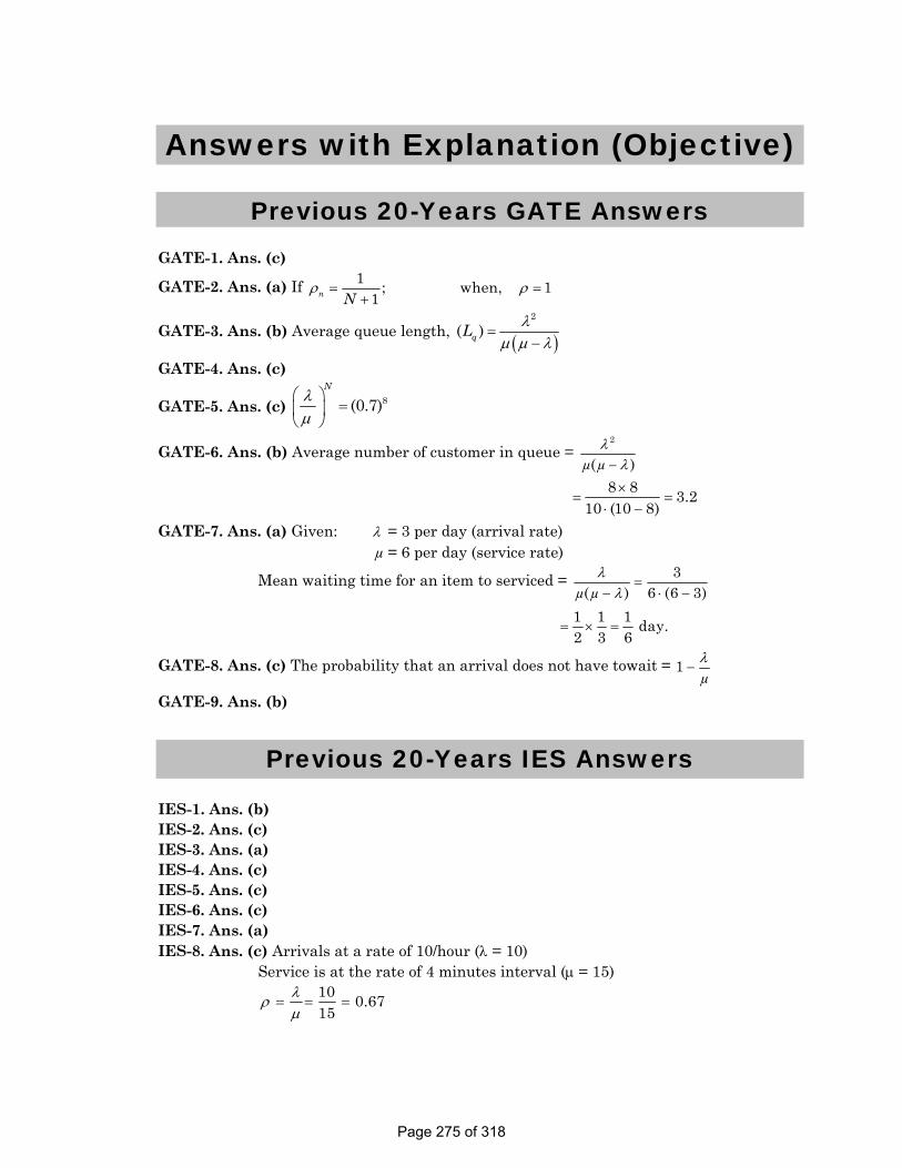
Queuing Model S K Mondal Chapter 16
Answers with Explanation (Objective)
Previous 20-Years GATE Answers GATE-1. Ans. (c)
GATE-2. Ans. (a) If ρ ρ= =+
1 ; when, 11n N
GATE-3. Ans. (b) Average queue length, ( )λ
μ μ λ=
−
2
( )qL
GATE-4. Ans. (c)
GATE-5. Ans. (c) λμ
⎛ ⎞=⎜ ⎟
⎝ ⎠8(0.7)
N
GATE-6. Ans. (b) Average number of customer in queue = 2
( )λ
λ−µ µ
×= =
⋅ −8 8 3.2
10 (10 8)
GATE-7. Ans. (a) Given: λ = 3 per day (arrival rate) µ = 6 per day (service rate)
Mean waiting time for an item to serviced = λλ
=− ⋅ −
3( ) 6 (6 3)µ µ
= × =1 1 1 day.2 3 6
GATE-8. Ans. (c) The probability that an arrival does not have towait = λ−1
µ
GATE-9. Ans. (b)
Previous 20-Years IES Answers
IES-1. Ans. (b) IES-2. Ans. (c) IES-3. Ans. (a) IES-4. Ans. (c) IES-5. Ans. (c) IES-6. Ans. (c) IES-7. Ans. (a) IES-8. Ans. (c) Arrivals at a rate of 10/hour (λ = 10) Service is at the rate of 4 minutes interval (μ = 15)
λρμ
= = =10 0.6715
Page 275 of 318

Queuing Model S K Mondal Chapter 16
per minutes
= perminutes
10
600.1666 1; 41 4
λ
ρ μ
=
=
IES-9. Ans. (d) Probability that person has to wait λρμ
= =
λ μ= = = =60 606 persons/hour and 10 persons/hour10 6
Therefore probability that person has to wait λμ
= = =6 0.6
10
IES-10. Ans. (c) IES-11. Ans. (c)
IES-12. Ans. (b) λλ μμ
= = = = = = =1 1 0.10.1, 0.25 and 0.4
10 4 0.25P
IES-13. Ans. (a) IES-14. Ans. (d) IES-15. Ans. (d) IES-16. Ans. (b)
IES-17. Ans. (b) Expected waiting time per customer in the system = λ
= ss
Lw
λμ λ λ μ λ
⎛ ⎞ ⎛ ⎞= =⎜ ⎟ ⎜ ⎟− −⎝ ⎠⎝ ⎠
1 1
IES-18. Ans. (d) 61.5
10 6
λμ λ
= =− −
IES-19. Ans. (a) Expected length of queue = ( )
λμ μ λ
= =− −
2 210 1.33( ) 15 15 10
IES-20. Ans. (a) IES-21. Ans. (a) Both A and R are true. Also R gives satisfactory explanation for A.
IES-22. Ans. (a) Mean arrival rate ( )λ = =1 6 customes arrivals/hr
Time of one arrival
Mean Service rate ( )μ = =1 15 custome service/hr
Time of one service
Probability that one has to wait ( ) λμ
= = =6 0.4
15P
IES-23. Ans. (c) λ 15Mean arrival rate, = = 1.5 customer / min10
μ
λμ
⎛ ⎞−⎜ ⎟
⎝ ⎠
10Mean service rate, = = 2 customer / min.5
Probability of idle = 1 = 0.25
Page 276 of 318

Queuing Model S K Mondal Chapter 16
IES-24. Ans. (a) λμ=
3Probability = 10
IES-25. Ans. (d) λμ
= = =15Utilization parameter 0.7520
λμ
= − =
=
Probability that system is idle 1 0.25
Probabilitythat a customer has to wait 0.75
IES-26. Ans. (a) IES-27. Ans. (b) IES-28. Ans. (a)
Page 277 of 318

Queuing Model S K Mondal Chapter 16
Conventional Questions with Answer Conventional Question [ESE-2004] In a machine shop certain type of machine breakdown are in accurate with Poisson process. The estimated cost of Idle machine is Rs. 15/-per hour. Two repair man A & B with different skill are being consider being haired as repairmen. Repairman a taken 6 min on an average to repair a machine and his wages are Rs. 8 per hour. When is repairman B taken 5 min to repair to and the wages are Rs. 10/- per hour. Which repairman should be used and why? Assume the work shift taken 8 hrs.
Solution: Consider A: Mean arrival rate (M) = 6
60 breakdown/min = 0.1 breakdown/min
Mean service time (µ) = 16
machine/min.
Mean waiting time of an arrival =⎛ ⎞−⎜ ⎟⎝ ⎠
110
1 1 16 6 10
= 9 min
In a day machine loss due to idle = × ×
× = −6 8 9Rs. 15 Rs. 108 /
60
Workman charge = Rs. 8 × 8 = Rs. 64/–
Total Cost = Rs. 172/–
Consider B: Mean arrival rate (M) = 660
breakdown/min = 0.1 breakdown/min
Mean service time (µ) = 1
5 repaire/min.
Mean waiting time of an arrival =( ) ( )μ μ
−
− − −= =
− −
1
1 1 1
10 5min5 5 10
MM
M/c Idle loss = × ×× = −
6 8 5 15 Rs. 60 /60
Man B charge = Rs. 8 × 10 = Rs. 80/–
Total Cost = Rs. 140/–
Use B workman. Example 1: Arrival of machinists at a tool crib are considered to be distributed as Poisson distribution with an average rate of 7 per hour. The service time at the tool crib is exponentially distributed with mean of 4 minutes. (a) What is the probability that a machinist arriving at the tool crib will have to wait? (b) What is the average number of machinists at the tool crib? (c) The company made a policy decision that it will install a second crib if a machinist
has to wait atleast five minutes before being served. What should be additional flow of machinist to the tool crib to justify a second tool crib?
Solution: Give λ = 7 per hour = 7
60 = 0.117 machinist per minute
Page 278 of 318
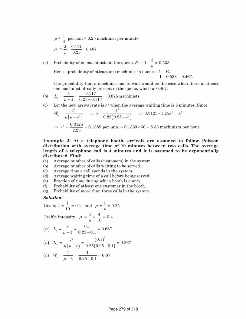
Queuing Model S K Mondal Chapter 16
µ = 14
per min = 0.25 machinist per minute
ρ = λ = =0.117 0.4670.25µ
(a) Probability of no machinists in the queue, Po = λμ
− =1 0.533
Hence, probability of atleast one machinist in queue = 1 – Po = 1 – 0.533 = 0.467.
The probability that a machinist has to wait would be the case when there is atleast one machinist already present in the queue, which is 0.467.
(b) λμ λ
= = =− −
0.117 0.875machinists.0.25 0.117sL
(c) Let the new arrival rate is λ1 when the average waiting time is 5 minutes. Since
( ) ( )λ λ λ λ
μ μ λ λ
λ
= ⇒ = ⇒ − =− −
⇒ = = = × =
1 11 1
1 1
1
5 0.3125 1.250.25 0.25
0.3125 0.1389 per min. 0.1389 60 8.33 machinists per hour.2.25
qW
Example 2: At a telephone booth, arrivals are assumed to follow Poisson distribution with average time of 10 minutes between two calls. The average length of a telephone call is 4 minutes and it is assumed to be exponentially distributed. Find: (a) Average number of calls (customers) in the system. (b) Average number of calls waiting to be served. (c) Average time a call spends in the system. (d) Average waiting time of a call before being served. (e) Fraction of time during which booth is empty. (f) Probability of atleast one customer in the booth. (g) Probability of more than three calls in the system.
Solution:
( )
( ) ( )( )( )
( )
λ μ
λρμ
λμ λ
λμ μ λ
μ λ
= = = =
= = =
= = =− −
= = =− −
= = =− −
22
1 1Given; 0.1 and 0.2510 4
4Traffic intensity, 0.410
0.1 0.6670.25 0.1
0.10.267
0.25 0.25 0.11 1 6.67
0.25 0.1
s
w
s
a L
b L
c W
Page 279 of 318

Queuing Model S K Mondal Chapter 16
( )
( )( ) ( )( ) ( ) ( ) ( ) ( )
( )
ρμ λρ
ρ ρ ρ ρ
= = =− −
= − = − =
> = − = − =
> = − + + = − + + = − + +
= − + + =
2 21 2
0.4 2.670.25 0.1
1 1 0.4 0.60 1 1 0.6 0.4
3 1 1 1 1
1 0.6 1 0.4 0.16 0.064
q
o
n o
n o o o o o
d W
e Pf P n P
g P n P P P P P P P
Example 3: A repair shop is manned by a single worker. Customers arrive at the rate of 30 per hour. Time required to provide service is exponentially distributed with mean of 100 seconds. Find the mean waiting time of a customer, needing repair facility in the queue.
Solution
( ) ( )
λ
μ
λμ μ λ
=×
= =
= = = =− −
Given; 30 per hour60 60 36 Customer per hour.
100Mean waiting time of a customer in the queue,
30 0.139 hour 8.33 minutes.36 36 30qW
Example 4: A commercial bank has three tellers counter for its customers. The services at these tellers are exponentially distributed with mean of 5 minutes per customer. The arrival of customers is Poisson distributed with mean arrival rate of 36 per hour. Analyses the system
Solution Given; λ = 36 per hour μ = 60
5 = 12 per hour
λμ= =
=
36 3124 tellers.C
( ) ( ) ( )
λ λ μμ μ μ λ
λ λ λ λ μμ μ μ μ μ λ
−
=
=⎡ ⎤ ⎡ ⎤⎛ ⎞ ⎛ ⎞
+⎢ ⎥ ⎢ ⎥⎜ ⎟ ⎜ ⎟ −⎝ ⎠ ⎝ ⎠⎢ ⎥ ⎢ ⎥⎣ ⎦ ⎣ ⎦
=⎡ ⎤ ⎡ ⎤⎛ ⎞ ⎛ ⎞ ⎛ ⎞ ⎛ ⎞ ⎛ ⎞+ + + +⎢ ⎥ ⎢ ⎥⎜ ⎟ ⎜ ⎟ ⎜ ⎟ ⎜ ⎟ ⎜ ⎟−⎝ ⎠ ⎝ ⎠ ⎝ ⎠ ⎝ ⎠ ⎝ ⎠⎢ ⎥ ⎢ ⎥⎣ ⎦ ⎣ ⎦
=⎡ ⎤×⎡ ⎤ ⎛ ⎞+ + + + ⎜ ⎟⎢ ⎥⎢ ⎥ × −⎣ ⎦ ⎝ ⎠⎣ ⎦
=+ + +
∑1
0
2 3 4
2 3 4
11 1! !
11 1 112 6 4!
11 1 1 12 41 3 3 3 32 6 24 12 4 36
11 3 4.5 4.
(i) o n CC
n
PC
n C C
CC
=+ +
0.03775 4.5 13.5
(ii) Average number of customers in the queue,
Page 280 of 318