www.lifeasti.eu

“Implementation of a forecAsting System for urban heaT Island effect for the development

of urban adaptation strategies” (LIFE ASTI)

Action A.1 Preliminary design of the pilot operational UHI forecasting systems

Thessaloniki December 2018

www.lifeasti.eu The project Implementation of a forecAsting System for urban heat Island effect for the development of urban adaptation strategies - LIFE ASTI has received funding from the LIFE Programme of the European Union”.

Document Information

Grant agreement number LIFE17 CCA/GR/OOO108

Project acronym LIFE ASTI

Project full title Implementation of a forecAsting System for urban heaT Island effect for the development of urban adaptation strategies

Project's website Under construction

Project instrument EUROPEAN COMMISSION - Executive Agency for Small and Medium-sized Enterprises

Project thematic priority Climate Change Adaptation

Deliverable type Report

Contractual date of delivery 31/12/2018

Actual date of delivery 31/12/2018

Deliverable title Preliminary Desing Report

Action A.1 Preliminary desing of the pilot operational UHI forecasting systems

Authors Christos Giannaros, Melas Dimitrios, Serafim Kontos, Stefania Argentini

Version History

Issue Date Version Author Partner

31-12-2018 V.9 Christos Giannaros, Melas Dimitrios, Serafim Kontos, Stefania Argentini

AUTh, ISAC-CNR

Disclaimer The sole responsibility for the content of this document lies with the authors. It does not necessarily reflect the opinion of the European Union. Neither the EASME nor the European Commission are responsible for any use that may be made of the information contained therein

Table of contents

I Preliminary Design Report ........................................................................................................................................... 4

i. Pilot UHI modeling system set-up .................................................................................................................... 5 a. Domains configuration ................................................................................................................................. 5 b. Meteorological initial and boundary conditions .......................................................................................... 6 c. Physics options ............................................................................................................................................. 6 d. Terrestrial and urban morphology input data ............................................................................................. 7 d.1. Land use/land cover .................................................................................................................................... 7 d.2. Topography ................................................................................................................................................. 8 d.3. Land surface and urban canopy parameters ............................................................................................... 8 e. Statistical downscaling algorithm ................................................................................................................ 9

ii. UHI-related forecasting products ................................................................................................................... 11 iii. Model evaluation data ................................................................................................................................... 13 iv. Climate and sensitivity simulations ................................................................................................................ 16 v. Local greening activities ................................................................................................................................. 17 References ............................................................................................................................................................... 18 Appendix A Calculation of UTCI ............................................................................................................................... 20

I Preliminary Design Report The LIFE ASTI project focuses on addressing the impact of Urban Heat Island (UHI) effect on human mortality by developing and evaluating a pilot system of numerical models that will lead to the short-term forecasting and future projection of the UHI phenomenon in two Mediterranean cities: Thessaloniki (Greece) and Rome (Italy). The phenomenon of UHI has an impact on human health, which is becoming more intense as the duration of the heat wave episodes is expected to increase due to climate change. The spread of urban areas has become alarming in recent years: almost 73% of Europe's population lives in cities, a rate which is expected to reach 80% by 2050. Extensive urbanization is triggering significant changes to the composition of the atmosphere and the soil, which result in the modification of the thermal climate and the temperature rise in urban areas, compared to neighboring nonurban ones. The modeling system which will be developed in the framework of the LIFE ASTI project, will produce high-quality forecasting products, such as bioclimatic indicators and heating and cooling degree days, which assess the energy needs of buildings. In addition, it will guide the Heat Health Warning System to be implemented in both cities and will aim at informing the competent authorities, the general population and the scientific community. The present document describes the preliminary design of the LIFE ASTI pilot numerical modeling system. More specifically, the Preliminary Design Report (PDR) includes the specification of the:

(a) Modeling system’s set-up covering essential aspects spanning from the configuration of the domains to the technique that will be applied for statistically downscaling selected forecasted products (Fig. 1).

(b) UHI-related forecasting products including mathematical equations that will be used in computational algorithms during the project’s implementation stage.

(c) Ground-based and satellite observational data that will be used for validating the outputs of the modeling system and statistical downscaling algorithm.

(d) Application of the modeling system for climate and sensitivity experiments in order to assess the impact of future climate change on UHI and quantify the effects of potential adaptation measures.

(e) Application of the modeling system based on local greening activities in order to demonstrate the effectiveness of the system in supporting UHI combating actions.

Figure 1. Flowchart of the pilot UHI modeling system

i. Pilot UHI modeling system set-up a. Domains configuration

Fig. 2 shows the WRF domains configuration that will be used in the framework of the LIFE ASTI project.

Figure 2. Configuration of the five (2-way) nested WRF modeling domains

The model will be applied over five (2-way) nested domains with spatial resolutions of 18 km (d01), 6 km (d02) and 2 km (d03, d04, d05). The first domain (d01; mesh size of 460x270 will cover most of the Europe, the North Africa

and the Middle East to simulate the synoptic meteorological conditions. The second domain (d02; mesh size of 450x345) includes the eastern Mediterranean, while two innermost domains focus on the studied urban areas of Thessaloniki, Greece, (d03; mesh size of 75x75) and Rome, Italy, (d05; mesh size of 78x45). All modeling domains will have the same vertical structure composing of 35 unevenly spaced full sigma layers from the lowest layer near the surface (~ 30 m) to the model top defined at 100 hPa. The above-described modeling technique is suitable for supporting the easy transferability and expandability of the system to any European and non-European region where UHI-related information is vital. For instance, the implementation of the eastern Mediterranean domain (d02) allows for including additional urban areas of the targeted, as well as of other, countries in the pilot UHI forecasting system. In this framework, the domain d04 (mesh size of 75x75) is targeted over the Heraklion, Crete, and will be used to test the transferability of the pilot UHI modeling system.

b. Meteorological initial and boundary conditions The modeling system will develop meteorological initial and boundary conditions for the coarse model grid (d01) based on forecast data produced by the Global Forecast System (GFS; http://www.emc.ncep.noaa.gov/GFS/doc.php). GFS is a global-scale weather prediction model created by the National Centers for Environmental Prediction (NCEP). Forecasts are made four times daily at 00:00, 06:00, 12:00 and 18:00 UTC providing various surface and upper-level atmospheric and land-soil variables at horizontal grid resolutions of 1.00°, 0.50° and 0.25°. In the current project, the GFS forecast data provided by the 12:00 UTC model cycle at 0.25°x0.25° (~ 27 km) spatial and 3 h temporal resolution over 32 vertical atmospheric layers and 4 soil layers will be used. The eastern Mediterranean domain (d02) will be initialized and forced at its lateral boundaries with meteorological fields interpolated from the coarse grid (d01). Correspondingly, the simulations over d02 will provide the atmospheric initial and boundary conditions to the two urban-scale domains (d03 and d04) targeted over the cities of Thessaloniki and Rome.

c. Physics options The WRF physics schemes include the: (a) microphysics, (b) cumulus physics, (c) planetary boundary and surface layer parameterizations, (d) land surface physics, and (e) short-wave and long-wave radiation parameterizations. Each category has multiple options varying from simple and efficient to more sophisticated and computationally costly. A considerable body of research has been implemented over the LIFE ASTI project studied regions examining the WRF performance in replicating hot summer conditions and the UHI effect (Giannaros T.M. and Melas, 2012, Giannaros T.M. et al., 2014; Giannaros C. et al., 2018, 2019; Morini et al., 2017). Based on these studies, the physics parameterizations listed in Table 1 will be applied in all modeling domains of the LIFE ASTI forecasting system.

Physics Parameterization References

Microphysics (clouds) WRF single-moment 5-class (WSM5)

Hong et al. (2004)

Cumulus (convection)* Kain-Fritsch (KF) Kain (2004) Planetary boundary layer asymmetric convection model

2 (ACM2) Pleim (2007a, 2007 b)

Surface layer Revised MM5 Jiménez et al. (2012)

Land surface Noah model Tewari et al. (2004) Short-wave radiation Dudhia Dudhia (1989)

Long-wave radiation rapid radiative transfer model for global circulation model (GCM) applications (RRTMG)

Iacono et al. (2008)

* Cumulus parameterization will be used only for domains d01 and d02 Table 1. Summary of the WRF physics options

Additionally, the Single-Layer Urban Canopy Model (SLUCM) will be coupled with the WRF model over Thessaloniki (d03) and Rome (d04) domains in order to represent in detail the physical processes of the targeted urban environments. The SLUCM (Kusaka et al., 2001; Kusaka and Kimura, 2004) simulates the effects of urban geomorphology on the dynamic, radiation and thermodynamic processes at the model sub-grid scale. It takes into account the cities land heterogeneity by distinguishing three types of urban surface: (a) industrial/commercial (IC), (b) high-intensity residential (HIR), and (c) low-intensity residential (LIR; Giannaros C. et al., 2018). Its application requires precise terrestrial and urban morphology data, including land use, topography and parameters representing the land surface and urban facets properties (e.g., surface albedo), as well as the urban canopy geometry (e.g., building heights).

d. Terrestrial and urban morphology input data

d.1. Land use/land cover The standard datasets used for representing the land use/land cover (LUCL) in the WRF model include the “moderate resolution imaging spectroradiometer (MODIS)” database with the classification of the “International Geosphere-Biosphere Project (IGBP)” and the “United States geological survey (USGS)” global dataset. The MODIS/IGBP dataset provides 20 land use/land cover categories in 30-arc-sec (~ 1 km) spatial resolution derived from the 2001 MODIS remote sensing products and modified for being used in the WRF modeling system. The USGS data include 24 types of LULC provided at 30-arc-sec horizontal grid resolution based on the 1-km “advanced very high resolution radiometer (AVHRR)” satellite images retrieved from April 1992 to March 1993. The USGS dataset is completely outdated, while both datasets are considered to be inadequate for urban-scale forecasting systems because they include only a single class (urban and built-up, UB) for representing urban environments. A more detailed urban LULC representation requires the employment of up-to-date and fine-scale datasets. Such datasets are available from the European Environmental Agency (EEA) in the framework of the “coordination of information on the environment (CORINE)” project (Giannaros C., 2018). In the framework of the LIFE ASTI project, the MODIS/IGBP dataset will be employed for representing the LULC in the domains d01 and d02. For the urban-scale domains d03 and d04, the LULC will be obtained from the 250 m spatial resolution CORINE 2012, version 18.5.1, dataset that includes 44 LULC categories. In order to be compatible with the WRF model, the CORINE data will be transformed to WPS (i.e., WRF pre-processor system) readable format adopting the following steps:

1. Download the CORINE data in raster (GeoTIFF) format from https://land.copernicus.eu/pan-european/corine-land-cover/clc-2012?tab=download.

2. Open the data with the open-source Geographical Information System (GIS) QGIS (https://www.qgis.org/en/site/) and: (a) Remap the 44 CORINE LULC categories to the corresponding MODIS/IGBP LULC classes according to

Pineda et al. (2004) and Giannaros T.M. et al. (2014; Table 1.2), (b) Reproject the data from their original European Terrestrial Reference System 1989 (ETRS89) Lambert

Azimuthal Equal Area (LAEA) to the WRF-compatible World Geodetic Coordinate System 1984 (WSG84),

(c) Convert the data from their original raster format to Ascii format.

3. Move the CORINE Ascii data in the WRF’s code directory “WPS/geogrid/src” and convert them into WPS format with the help of the “write_geogrid.c” Fortran routine (see http://forum.wrfforum.com/viewtopic.php?f=22&t=2266 for more details).

As shown in Table 2, the CORINE data enable the three additional urban LULC categories (IC, HIR, LIR) that are necessary for implementing the SLUCM (Giannaros C, 2018).

CORINE urban LULC classification MODIS/IGBP urban LULC classification

1.1.1: Continuous urban fabric 32: High-intensity residential 1.1.2: Discontinuous urban fabric 31: Low-intensity residential 1.2.1: Industrial/commercial units 33: Industrial/commercial 1.2.2: Road/rail networks and associated land 13: Urban and built-up 1.2.3: Port areas 13: Urban and built-up 1.2.4: Airports 13: Urban and built-up 1.3.1: Mineral extraction sites 13: Urban and built-up 1.3.2: Dump sites 13: Urban and built-up 1.3.3: Construction sites 13: Urban and built-up 1.4.1: Green urban areas 31: Low-intensity residential 1.4.2: Sports and leisure facilities 31: Low-intensity residential

Table 2. Mapping strategy of the CORINE urban LULC elements to the corresponding WRF urban LULC categories

d.2. Topography By default, the topography is represented in the WRF modeling system using the 30-arc-sec spatial resolution USGS terrain dataset. This dataset will be applied over the coarse- and moderate-resolution domains d01 and d02 of the LIFE ASTI pilot forecasting system. Concerning the fine-scale domains, several studies highlighted that the integration of high-resolution terrain data in the WRF model, such as those of the Shuttle Radar Topography Mission (SRTM) dataset (Farr et al., 2007), improve remarkably its performance in simulating the near-surface meteorological fields (e.g., Lupascu et al., 2015; Meij and Vinuesa, 2014; Nunalee et al., 2015). For this, the 250 m horizontal grid resolution resampled SRTM topography data, version 4.1 (Jarvis et al., 2008), will be utilized over the LIFE ASTI domains d03 and d04. The data will be downloaded from http://gisweb.ciat.cgiar.org/TRMM/SRTM_Resampled_250m/ in raster (GeoTIFF) format and will be converted to WPS-compliant format using QGIS and a command line utility based on the Geospatial Data Abstraction Library (GDAL;https://www.gdal.org/) and the programming language Python (https://www.python.org/; see https://wrfexplorer.wordpress.com/2015/03/24/high-resolution-topography/ for more details).

d.3. Land surface and urban canopy parameters Land surface properties have a crucial role in urban modeling applications because they contribute to the accurate representation of the surface energy budget (SEB). Especially, the surface albedo and emissivity are of great importance in the UHI causation and development. In addition, the implementation of the SLUCM requires the realistic description of the urban environment through the specification of 20 urban canopy parameters (UCPs) for each urban LULC category (IC, HIR, LIR). Among the UCPs, the building height and road width are marked with high significance in representing the complex geometry of the urban street canyons, while the urban fraction (i.e., the percentage of the impervious urban facets in the WRF sub-grid proportion) affects essentially the near-surface air temperatures (Giannaros C., 2018). The adaptation of these highly uncertain land surface and urban canopy properties for Thessaloniki and Rome is a necessary procedure in order to conclude to an optimal set of parameters, which is representative of the targeted cities.

The specification of the surface albedo and emissivity over the studied areas will be based on satellite-retrieved data. In particular, albedo and emissivity maps for Thessaloniki and Rome will be obtained from the new Sentilel-2 satellite during action C.3 and will be integrated in the pilot UHI forecasting system. Following Giannaros C. et al. (2018) methodology, the SLUCM code will be modified to assign the retrieved values of albedo and emissivity to the pervious and impervious, including roads, walls and roofs, surfaces of each urban grid cell. Concerning the building height, road width and urban fraction, the values of these variables for Thessaloniki and Rome will be set equal to those applied in the study of Giannaros C. et al. (2018) for the city of Athens. Thessaloniki is characterized by a similar urban structure as Athens and, thus, it is foreseen that the adoption of Athens’ UCPs will be representative for the city. For Rome, the values will be calibrated, if necessary, based on the evaluation of the model results during action C.3.

e. Statistical downscaling algorithm The ultimate goal for UHI modeling systems is to capture the intra-urban variations of near-surface meteorological variables associated with the thermal environment on the scale of few hundreds of meters. This requires the application of the system with high horizontal grid resolution; in principle lower than 1 km. However, this is not always possible, especially in operational forecasting systems, due to limitations in the availability of computational resources. In order to address this issue, statistical downscaling can be applied as an alternative method for producing high-resolution forecasts without increasing computer resource requirements (Giannaros T.M. et al, 2014). In this case, the local climate is predicted through statistical relationships that combine the model forecasts with fine-scale historical observations and various parameters that govern the variability of the meteorological fields (e.g., topography; Fig. 3).

Figure 3. Schematic example of a statistical downscaling case (adopted from

https://meteo.unican.es/downscaling/intro.html#) Nowadays, there is a variety of statistical downscaling methods, which are divided into three categories: analogs and weather typing, stochastic weather generators and regression models that are based on linear or non-linear relationships (Benestad et al., 2008). The regression approach is the most widely used method due to its relatively easy realization and its relatively small computational needs (Tang et al., 2016). Linear regression has been applied successfully in several studies involving regional climate models, especially for temperature estimations. However, this method is limited by its assumption that the dependent (output) variable has a linear relationship with each independent (input) variable (Le Roux et al., 2017). For this, a non-linear regression technique will be used in the current project in order to downscale selected 2-km forecasted products derived from the urban-scale domains

(d03 over Thessaloniki and d04 over Rome) to the spatial resolution of the SRTM topography and CORINE LULC grid (i.e., 250 m). In particular, the LIFE ASTI statistical downscaling algorithm (LASDA) will be based on Support Vector Regression (SVR) to predict the 2-m air temperature and relative humidity at 250 m horizontal grid resolution over Thessaloniki and Rome. SVR is capable of handling large amount of multidimensional data without requiring significant amounts of computation time. It is based on machine learning theory utilizing Kernel functions to estimate complex and multivariate relationships between a dependent variable (i.e., predicted named as Y) and a range of independent variables (i.e., predictors named as X; Le Roux et al., 2018). The selection of the input predictors is based on the predictive power that believed to have over the output predicted variable, while the selection of the Kernel function defines the statistical assumption used for estimating the relationship between the variables. LASDA will be developed using the LIBSVM tools, version 3.23, developed by Chang and Lin (2013; freely available on GitHub: https://github.com/cjlin1/libsvm). The radius basis function (RBF) Kernel will be used, as it is one of the most frequently applied Kernel function accounting for non-linear problems and is known to perform well in earth science applications (e.g., Du et al., 2017; Kim et al., 2018; Le Roux et al., 2018). The input data will include (a) the geographical coordinates (latitude and longitude) the impact of location on the predicted variables, (b) the time of the day, separated into two components using the sine and cosine trigonometric functions, to represent the diurnal cycle of the predicted variables, (c) the 250 m spatial resolution SRTM terrain elevation data to describe the effect of topography on the predicted variables, (d) the 250 m spatial resolution CORINE LULC data to represent the impact of land surface type on the predicted variables, and (e) the 2-km simulated data. The expected output will be the modeled data downscaled to 250 m spatial resolution. The implementation of LASDA will be based on the procedure suggested by the LIBSVM guide (Hsu et al., 2016). More specifically, the following steps will be adopted:

1. Prepare the data on the appropriate LIBSVM format. 2. Scale the data to equalize quantitative differences among them. 3. Apply a grid search routine and 5-fold cross validation for selecting the optimal parameters for LASDA’s

equation. 4. Train the LASDA using the optimal parameters found in step 3. 5. Test the trained LASDA to assess the predictive accuracy of the algorithm

LASDA training and testing will be carried out in two phases using ground-based observational data of 2-m air temperature and relative humidity. The first stage will be completed prior the beginning of the early pilot UHI forecasting system operation (May 2019; action C.2) using 2015 warm period (May to September) measurements collected from existing networks of weather stations in Thessaloniki and Rome. The second phase will take place in parallel with the evaluation of the pilot UHI modeling system during action C.3 in order to refine the initially developed LASDA. In this case, the training and testing period will be the warm season of 2019 using observations provided by the existing measurement networks, as well as by the additional urban weather stations that will be installed in both targeted cities during action A.2. For Thessaloniki, measurements from a micro-sensor monitoring network that will be installed in the framework of KASTOM project will be also utilized (more details on the validation data are provided in section 3). In both stages, three training datasets (i.e., one for 2-m air temperature, one for 2-m dew point temperature and one for 2-m air relative humidity) will be constructed for each studied city. The learning datasets will consist of:

(a) hourly observations at the locations of various meteorological stations within each targeted urban area (LASDA “desired output”),

(b) geographical coordinates of each meteorological station (LASDA input), (c) time of the day, transformed using the sine and cosine trigonometric functions (LASDA input), (d) terrain elevation of each meteorological station according to the 250 m spatial resolution SRTM dataset

(LASDA input),

(e) land use classification of each meteorological station according to the 250 m spatial resolution CORINE LULC dataset (LASDA input),

(f) hourly 2-km simulated data, bilinearly interpolated onto the locations of the meteorological stations (LASDA input).

The respective testing datasets will have the same composition apart from the “desired output”. During the testing, the output will be resulted from the LASDA application and it will be compared against the ground-based measurements by computing statistical measures, such as the mean bias (MB), the mean absolute error (MAE) and the index of agreement (IOA). Following the LASDA validation, the algorithm will be applied as a post-processing step after the implementation of the pilot UHI forecasting system (see “post-processing tools” in section 2) resulting to 250 m spatial resolution 2-m air temperature and relative humidity over Thessaloniki and Rome.

ii. UHI-related forecasting products The UHI forecasting system will be initialized at 19:00 local time on a daily basis during its pilot implementation. 96 h numerical simulations will be conducted providing output in netCDF format every hour. The first 12 simulated hours will be discarded from the forecasts because they will be coincided with the model’s spin up period. A dedicated database, named as pilot operational simulations database (POSD), will be created to store systematically the UHI forecasting system’s output. Post-processing tools (PPTs) applied to the POSD’s data will be developed based on advanced programming languages, such as Python and NCL (National Center of Atmospheric Research (NCAR) command language). PPTs will be used for extracting and computing the UHI-related prediction products, most of which will be provided to the end-users through the LIFE ASTI system platform (LASP; see the Architectural and Functional Report (AFR) for more details). More specifically, the LIFE ASTI forecasting products will include: • The 2-m air temperature at 250 m spatial resolution (T2_250m) in °C provided through the application of

the LASDA. • The 2-m air relative humidity at 250 m spatial resolution (RH2_250m) in % provided through the

application of the LASDA. • The 2-m dew point temperature at 250 m spatial resolution (TD2_250m) °C calculated using the following

formula:

SVP_250m = 6.11 ∙ 107.5∙T2_250m

237.7+T2_250m (2.1a)

VP_250m =RH_250m ∙ SVP_250m

100 (2.1b)

TD2_250m =237.7 ∙ ln (SVP_250m

6.11)

7.5 − ln (SVP_250m6.11

) (2.1c)

where SVP_250m and SV_250m are the saturated and actual vapor pressure at 250 m horizontal grid resolution, respectively, in hPa.

• The 10-m wind speed and direction at 2 km horizontal grid resolution (WS10_2km and WD10_2km) in m/s and °, respectively.

• The downward short-wave solar radiation at 2k horizontal grid resolution (SW_2km) in W/m2. • The downward long-wave solar radiation at 2k horizontal grid resolution (LW_2km) in W/m2.

• The UHI intensity at 250 m spatial resolution (UHII_250m) in °C defined as the T2_250m difference between an urban area and a surrounding territory, which is representative of non-urban conditions (e.g., rural):

UHII_250m = T2_250murban − T2_250mnon−urban (2.2)

It should be noticed that the selected urban and non-urban areas must have common topographic features to eliminate temperature divergences associated mainly with the terrain elevation (Giannaros C., 2018).

• The discomfort index at 250 m horizontal grid resolution (DI_250m) in °C calculated using the following equation:

DI_250m = T2_250m − 0.55 ∙ (1 − 0.01 ∙ RH_250m) ∙ (T2_250m − 14.5) (2.3)

DI_250m provides a measure of discomfort experienced by an individual according to Table 3 (Giannaros T.M. et al., 2014).

DI value Discomfort conditions

DI ≤ 21 °C No discomfort 21 °C < DI ≤ 24 °C Under 50 % of the population feels discomfort 24 °C < DI ≤ 27 °C Above 50 % of the population feels discomfort 27 °C < DI ≤ 29 °C Most of the population feels discomfort 29 °C < DI ≤ 32 °C The entire population feels discomfort DI > 32 °C Sanitary emergency conditions

Table 3. The discomfort index assessment scale • The universal thermal climate index at 250 m spatial resolution (i.e., the highest horizontal grid

resolution of the inputs; UTCI_250m) in °C estimated by a 6th order polynomial regression equation, which considers the effects of near-surface air and dew point temperature, relative humidity, wind speed and radiation on thermal comfort (http://www.utci.org/utci_doku.php; see Appendix A). Table 4 provides the thermal sensation associated with the UTCI values (Giannaros T.M., 2013).

UTCI value Thermal sentation

UTCI ≤ – 40 °C Extreme cold stress – 40 °C < UTCI ≤ – 27 °C Very strong cold stress – 27 °C < UTCI ≤ – 13 °C Strong cold stress – 13 °C < UTCI ≤ 0 °C Moderate cold stress 0 °C < UTCI ≤ 9 °C Slight cold stress 9 °C < UTCI ≤ 26 °C No thermal stress (comfort) 26 °C < UTCI ≤ 32 °C Moderate heat stress 32 °C < UTCI ≤ 38 °C Strong heat stress 38 °C < UTCI ≤ 46 °C Very strong heat stress UTCI > 46 °C Extreme heat stress

Table 4. The UTCI assessment scale • The apparent temperature at 250 m horizontal grid resolution (TAPP_250m) in °C computed based on the

following equation: TAPP_250m = −2.653 + 0.994 ∙ T2_250m + 0.0153 ∙ (TD2_250m)2 (2.4)

TAPP_250m will be used in developing and operating the pilot heat health warning system (HHWS) during action C.6 (Michelozzi et al., 2010).

• The daily value of cooling and heating degree days at 250 m spatial resolution (CDD_250m, HDD_250m) in °C days calculated using the equation:

CDD_250m = (1 day) ∙ (T2_250mmean − T2base_cdd) (2.5) HDD_250m = (1 day) ∙ (T2_250mmean − T2base_hdd) (2.5)

where T2_250mmean is the daily mean T2_250m, and T2base_cdd = 22 °C and T2base_hdd = 15.5 °C is the base temperature for cooling and heating, respectively. CDD_250m (HDD_250m) will be used as measure that reflect (proportionally) the energy demand to cool (heat) a building to a comfortable temperature (Elizbarashvili et al., 2018; Spinoni et al., 2014).

It is worth mentioning that the selection of downscaling only 2-m air temperature and relative humidity at 250 m horizontal grid resolution derives from the fact that the rest of the forecasting variables do not vary significantly at the scale of the LIFE ASTI urban domains that focus over the studied areas (i.e., 2 km).

iii. Model evaluation data The evaluation of the pilot UHI forecasting system will take place after its first pilot application in the framework of action C.3. Satellite and in-situ observations from existing and additional measurement networks will be utilized for this purpose. For Thessaloniki, the observational data will be collected from ground-based weather stations operated by the Municipality of Thessaloniki (MoT), Region of Central Macedonia (RCM), National Hellenic Meteorological Service (HNMS) and Aristotle University of Thessaloniki (AUTH). Table 5 presents the main characteristics of the measurement sites classified into local climate zones (LCZs) according to Stewart and Oke (2012), while Fig. 4 illustrate their locations.

Monitoring network

Station name (short name)

Latitude (°N) Longitude (°E) Altitude (m a.s.l.a)

LCZ classification

MoT

Eptapyrgio (EPT) 40.64 22.94 43 2: Compact mid-rise Pedio tou Arews (PAR) 40.62 22.96 13 2: Compact mid-rise 25is Martiou (MAR) 40.60 22.96 20 2: Compact mid-rise Lagada (LAG) 40.65 22.94 45 2: Compact mid-rise

RCM

Kalamaria (KAL) 40.58 22.96 61 5: Open mid-rise Kordelio (KOR) 40.67 22.89 31 2: Compact mid-rise Panorama (PAN) 40.59 23.03 364 6: Open low-rise Sindos (SIN) 40.66 22.80 2 9: Sparsely built

HNMS Makedonia Airport (AIR)

40.52 22.97 6.7 8: Large low-rise

AUTH AUTH (AUTH) 40.63 22.96 39 2: Compact mid-rise

LIFE ASTI

Evosmos (EVO) 40.67 22.91 30 2: Compact mid-rise Agias Sofias (AGS) 40.63 22.95 22 2: Compact mid-rise Toumpa-Xarilaou-Triandria (TXT)

40.61 22.96 24 2: Compact mid-rise

a above sea level Table 5. Major characteristics of the ground-based observational sites over Thessaloniki

Three stations, namely EVO, AGS and TXT, refer to the supplementary urban weather sites that will be installed during action A.2 in order to increase the spatial coverage of the current monitoring networks. Additional data will be obtained from a dense micro-sensor network that will be installed and operated from May 2019 during the

project “Innovative system for air quality monitoring and forecasting” (KASTOM). KASTOM is funded by the European Regional Development Fund under the “Competitiveness, Entrepreneurship and Innovation” (EPAnEK) Operation Programme 2014-2020 and coordinated by AUTH, which is also the LIFE ASTI coordinator.

Figure 4. Locations of Thessaloniki’s ground-based weather stations (green color denoted MoT network, blue color denotes RCM network, pink color denotes HNMS network, light blue denotes AUTH network and red color denotes

LIFE ASTI network). In Rome, two existing weather station networks, already operational (Fig. 5, red flags), will be exploited for collecting data for the evaluation of the model; the first is managed by the Regional Agency for the Environmental Protection (ARPA Lazio) whereas the second by Meteo Lazio, an amateur network, responding to the WMO standards. The ARPA Lazio stations are micro-meteorological stations equipped with the following instrumentation: (a) a three-axes ultrasonic thermometer-anemometer USA-1 (Metek Scientific), (b) a radiometric station CNR1 (Kipp & Zonen), (c) a thermo-hygrometer HMP155 (Vaisala), (d) a barometer PTB 110 (Vaisala), (e) a rain gauge C100A (LASTEM), (f) sensors for measurements of the thermal properties of the ground, (g) a soil flux plate at 5 cm depth and (h) soil sensors for temperature measures at 2.5, 5.0, 10.0 and 50 cm. The Meteo Lazio stations are Davis Vantage Pro2™ Wireless Weather Stations providing measurements of the main meteorological parameters such as temperature, relative humidity, precipitation, wind speed and direction.

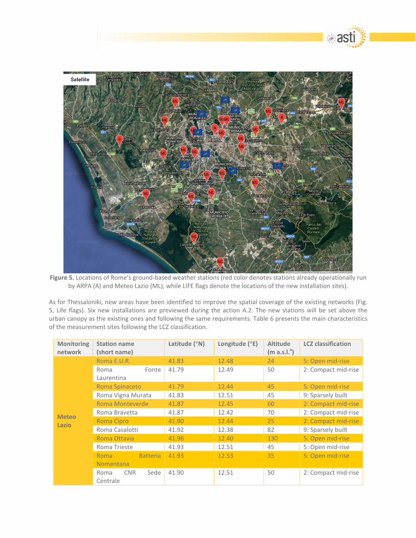
Figure 5. Locations of Rome’s ground-based weather stations (red color denotes stations already operationally run

by ARPA (A) and Meteo Lazio (ML), while LIFE flags denote the locations of the new installation sites). As for Thessaloniki, new areas have been identified to improve the spatial coverage of the existing networks (Fig. 5, Life flags). Six new installations are previewed during the action A.2. The new stations will be set above the urban canopy as the existing ones and following the same requirements. Table 6 presents the main characteristics of the measurement sites following the LCZ classification.

Monitoring network

Station name (short name)

Latitude (°N) Longitude (°E) Altitude (m a.s.l.a)

LCZ classification

Meteo Lazio

Roma E.U.R. 41.83 12.48 24 5: Open mid-rise Roma Fonte Laurentina

41.79 12.49 50 2: Compact mid-rise

Roma Spinaceto 41.79 12.44 45 5: Open mid-rise Roma Vigna Murata 41.83 12.51 45 9: Sparsely built Roma Monteverde 41.87 12.45 60 2: Compact mid-rise Roma Bravetta 41.87 12.42 70 2: Compact mid-rise Roma Cipro 41.90 12.44 25 2: Compact mid-rise Roma Casalotti 41.92 12.38 82 9: Sparsely built Roma Ottavia 41.96 12.40 130 5: Open mid-rise Roma Trieste 41.93 12.51 45 5: Open mid-rise Roma Batteria Nomentana

41.93 12.53 35 5: Open mid-rise

Roma CNR Sede Centrale

41.90 12.51 50 2: Compact mid-rise

Roma Tor Sapienza 41.91 12.59 32 9: Sparsely built Roma Tor De Schiavi 41.89 12.56 35 5: Open mid-rise Roma Centocelle 41.88 12.56 45 2: Compact mid-rise Settecamini 41.94 12.63 55 9: Sparsely built Ciampino 41.81 12.59 105 9: Sparsely built Castel Romano 41.71 12.45 85 9: Sparsely built Dragona 41.79 12.33 25 9: Sparsely built Fosso Olgiata 42.05 12.36 155 B: Scattered trees Fonte Di Papa 42.05 12.57 40 C: Bush, scrub Tivoli 41.96 12.80 253 2: Compact mid-rise

ARPA Lazio

Tor Vergata 41.84 12.65 100 9: Sparsely built Castel Di Guido 41.89 12.27 70 B: Scattered trees Roma Boncompagni 41.91 12.50 72 2: Compact mid-rise Cavaliere 41.93 12.66 57 G: Water

LIFE ASTI

Appia antica 41.83 12.54 83 B: Scattered trees Università Salesiana 41.96 12.52 55 5: Open mid-rise Liceo Orazio 41.94 12.55 40 5: Open mid-rise Liceo Keplero Centrale 41.86 12.47 20 2: Compact mid-rise Liceo Keplero Succursale

41.84 12.42 60 9: Sparsely built

Città Del Vaticano 41.90 12.45 35 5: Open mid-rise Tor Vergata 41.84 12.65 100 9: Sparsely built Zona Municipio XV 41.94 12.46 20 5: Open mid-rise

a above sea level Table 6. Major characteristics of the ground-based observational sites over Rome

For both cities, the retrieved data will include hourly values of near-surface meteorological parameters, primarily air temperature and relative humidity. The data will be converted in usable format and will be stored on a dedicated database, the ground-based and remote-sensing database (GROD). Advanced programming languages (e.g., Python, NCL) will be used for developing statistical analysis tools (SATs), which will be applied for comparing the forecasting system’s output against the ground-based observations focusing on the UHI-related products (see section 2). For example, key statistical measures (e.g., MB, MAE, IOA) will be calculated. The evaluation data will cover the period from May to September 2015 and 2019. The 2015 data will be used for the first phase of LASDA training and testing (see sub-section 1.5). The 2019 data will be used for evaluating the performance of the pilot UHI forecasting system, as well as for validating the LIFE ASTI statistical downscaling algorithm (see sub-section 1.5). Moreover, hourly land surface temperature (LST) maps for the two studied cities will be retrieved from the geostationary satellite MSG2-SEVIRI and the new Sentinel-2 satellite. They will cover one week of the 2019 warm period (May to September) and will be stored on the GROD. The remote-sensed LST maps will be used for qualitatively comparing them against the model simulated LST.

iv. Climate and sensitivity simulations The pilot UHI forecasting system will be applied for climate simulations and sensitivity experiments during action C.4. For this objective, the modeling system will be initialized and forced at its lateral boundaries with the global bias-corrected climate model output from NCAR's Community Earth System Model, version 1, (CESM1) that participated in phase 5 of the Coupled Model Intercomparison Experiment (CMIP5) supporting the Intergovernmental Panel on Climate Change Fifth Assessment Report (IPCC AR5). The data are available online (https://rda.ucar.edu/datasets/ds316.1/) provided in WPS-compliant format at 26 pressure levels and 6 hourly

intervals and. They are bias-corrected using the European Centre for Medium-Range Weather Forecasts (ECMWF) Interim Reanalysis (ERA-Interim) fields for 1981-2005 (Monaghan et al., 2014). Using the same model set-up (see section i) and the CESM1-CMIP5 data as initial and boundary conditions for the coarse model grid (d01), the following simulations will be performed:

(a) A control simulation (base case scenario), which refers to the 20th century representing the present climate conditions.

(b) Two climate simulations (future climate scenarios) projecting the short-term (until 2050) and distant (between 2051 and 2100) future conditions. The simulations will be based on the next generation of scenario simulations, the so-called Reference Concentration Pathways (RCPs), i.e., prescribed GreenHouse-Gas (GHG) concentration pathways throughout the 21st century, corresponding to different radiative forcing stabilization levels by the year 2100.

(c) Two sensitivity simulations (sensitivity experiments) introducing UHI adaptation measures in the base case scenario. Green and cool roofs, as well as green infrastructures (e.g., parks), will be introduced during these simulations by replacing and modifying the properties (e.g., albedo) of roofs and land use in specific urban grid points of the model over Thessaloniki (d03) and Rome (d04). The exact grid points, where the modifications will take place in the sensitivity simulations, will be determined based on the spatial distribution of the UHI magnitude and thermal discomfort, as well as considering the suitability of a place regarding green interventions. In particular, it is foreseen that areas characterized by high UHI intensity and thermal discomfort, and considerable potential for greening expansion will be chosen

The simulations’ outcome will be stored on a dedicated Assessment Simulations Database (ASD). The future climate scenarios will be compared with the base case scenario in order to assess the impact of the RCP8.5 future climate change scenario on UHI and energy demands of buildings (based on CDD). The sensitivity experiments will also be compared with the base case scenario in order to determine the effect of the selected UHI adaptation strategies and quantify their benefits. Several investigation methodologies will be applied, including statistical analysis, and thematic maps, to cover all aspects of the UHI and adaptation plans assessment under climate change conditions.

v. Local greening activities Sensitivity simulations based on local greening activities will be conducted using the pilot UHI forecasting system in the framework of action C.7. In Thessaloniki, the simulations will be carried out for green actions that have been applied in practical terms. Indicatively, MoT has already completed green intervations such as the bioclimatic upgrading of the Stock Exchange Square wider area, the improvement of the microclimate conditions in Stamatis Karamanlis square and the formulation of four school curves based on bioclimatic criteria. These actions include the coating of green and cool materials and new plantings. For Rome, the simulations will be implemented for hypothetical green activities having an analogous spatial scale as the corresponding actions in Thessaloniki. Following a similar technique as in the case of the climate sensitivity experiments (Section iv), the land use in the modeling system will be adapted according to the changes in the cities’ intervention areas. The sensitivity simulations will cover the summer period (June to August) of 2020. Quantitative and qualitative analysis will be applied for comparing the sensitivity experiments’ results with those that will be resulted from the June-August 2020 pilot application of the UHI forecasting system. In addition, a survey/questionnaire will be given to to a pool of residents of the locations where adaptation actions plans applied in order to monitor the real impact on their thermal comfort conditions. In this way, the effect of the local green measures in terms of combating the UHI effect and its impacts on human health and energy demand will be assessed. Moreover, the local green actions will

be the base for designing and assessing larger-scale interventions. Thus, the effectiveness of the modeling system regarding the support of developing and validating UHI adaptation activities will be examined.

References Benestad, R.E., Hanssen-Bauer, I., Chen, D., 2008. Empirical-Statistical Downscaling. WORLD SCIENTIFIC. doi:doi:10.1142/6908. Chang, C-C., Lin, C-J., 2013. LIBSVM: A library for support vector machines Technical report, Department of Computer Science, National Taiwan University. https://www.csie.ntu.edu.tw/~cjlin/papers/libsvm.pdf. Chih-Wei Hsu, Chih-Chung Chang, Lin, C.-J., Chih-Wei Hsu, Chih-Chung Chang, and C.-J.L., Chih-Wei Hsu, Chih-Chung Chang, Lin, C.-J., 2008. A Practical Guide to Support Vector Classification. BJU Int. 101, 1396–1400. doi:10.1177/02632760022050997. De Meij, A., Vinuesa, J.F., 2014. Impact of SRTM and Corine Land Cover data on meteorological parameters using WRF. Atmos. Res. 143, 351–370. doi:10.1016/j.atmosres.2014.03.004. Du, J., Liu, Y., Yu, Y., Yan, W., 2017. A prediction of precipitation data based on Support Vector Machine and Particle Swarm Optimization (PSO-SVM) algorithms. Algorithms 10. doi:10.3390/a10020057. Dudhia, J., 1989. Numerical Study of Convection Observed during the Winter Monsoon Experiment Using a Mesoscale Two-Dimensional Model. J. Atmos. Sci. 46, 3077–3107. doi:10.1175/1520-0469(1989)046<3077:NSOCOD>2.0.CO;2. Elizbarashvili, M., Chartolani, G., Khardziani, T., 2018. Variations and trends of heating and cooling degree-days in Georgia for 1961–1990 year period. Ann. Agrar. Sci. 16, 152–159. doi:10.1016/j.aasci.2018.03.004. Farr, T.G., Rosen, P.A., Caro, E., Crippen, R., Duren, R., Hensley, S., Kobrick, M., Paller, M., Rodriguez, E., Roth, L., Seal, D., Shaffer, S., Shimada, J., Umland, J., Werner, M., Oskin, M., Burbank, D., Alsdorf, D., 2007. The Shuttle Radar Topography Mission. Rev. Geophys. 45. doi:10.1029/2005RG000183. Giannaros, C., Melas, D., Giannaros, T.M., 2019. On the short-term simulation of heat waves in the Southeast Mediterranean: Sensitivity of the WRF model to various physics schemes. Atmos. Res. 218, 99–116. doi:https://doi.org/10.1016/j.atmosres.2018.11.015. Giannaros, C., Nenes, A., Giannaros, T.M., Kourtidis, K., Melas, D., 2018. A comprehensive approach for the simulation of the Urban Heat Island effect with the WRF/SLUCM modeling system: The case of Athens (Greece). Atmos. Res. 201, 86–101. doi:https://doi.org/10.1016/j.atmosres.2017.10.015. Giannaros, T.M., Melas, D., 2012. Study of the urban heat island in a coastal Mediterranean City: The case study of Thessaloniki, Greece. Atmos. Res. 118, 103–120. doi:10.1016/j.atmosres.2012.06.006. Giannaros, T.M., Melas, D., Daglis, I.A., Keramitsoglou, I., 2014. Development of an operational modeling system for urban heat islands: An application to Athens, Greece. Nat. Hazards Earth Syst. Sci. 14, 347–358. doi:10.5194/nhess-14-347-2014. Hong, S.-Y., Dudhia, J., Chen, S.-H., 2004. A Revised Approach to Ice Microphysical Processes for the Bulk Parameterization of Clouds and Precipitation. Mon. Weather Rev. 132, 103–120. doi:10.1175/1520-0493(2004)132<0103:ARATIM>2.0.CO;2.

Iacono, M.J., Delamere, J.S., Mlawer, E.J., Shephard, M.W., Clough, S.A., Collins, W.D., 2008. Radiative forcing by long-lived greenhouse gases: Calculations with the AER radiative transfer models. J. Geophys. Res. Atmos. 113, 2–9. doi:10.1029/2008JD009944. Jarvis, A., Reuter, H.A., Nelson, A., Guevara, E., 2008. Hole-filled seamless SRTM data V4. International Centre for Tropical Agriculture (CIAT). http://srtm.csi.cgiar.org (last accessed February 2017). Jiménez, P. a., Dudhia, J., González-Rouco, J.F., Navarro, J., Montávez, J.P., García-Bustamante, E., 2012. A Revised Scheme for the WRF Surface Layer Formulation. Mon. Weather Rev. 140, 898–918. doi:10.1175/MWR-D-11-00056.1. Kain, J.S., 2004. The Kain–Fritsch Convective Parameterization: An Update. J. Appl. Meteorol. 43, 170–181. doi:10.1175/1520-0450(2004)043<0170:TKCPAU>2.0.CO;2. Kim, D., Moon, H., Kim, H., Im, J., Choi, M., 2018. Intercomparison of Downscaling Techniques for Satellite Soil Moisture Products. Adv. Meteorol. 2018. doi:10.1155/2018/4832423. Kusaka, H., Kimura, F., 2004. Coupling a Single-Layer Urban Canopy Model with a Simple Atmospheric Model: Impact on Urban Heat Island Simulation for an Idealized Case. J. Meteorol. Soc. Japan 82, 67–80. doi:10.2151/jmsj.82.67. Kusaka, H., Kondo, H., Kikegawa, Y., Kimura, F., 2001. A Simple Single-Layer Urban Canopy Model For Atmospheric Models: Comparison With Multi-Layer And Slab Models. Boundary-Layer Meteorol. 101, 329–358. doi:10.1023/A:1019207923078. Le Roux, R., de Rességuier, L., Corpetti, T., Jégou, N., Madelin, M., van Leeuwen, C., Quénol, H., 2017. Comparison of two fine scale spatial models for mapping temperatures inside winegrowing areas. Agric. For. Meteorol. 247, 159–169. doi:10.1016/j.agrformet.2017.07.020. Le Roux, R., Katurji, M., Zawar-Reza, P., Quénol, H., Sturman, A., 2018. Comparison of statistical and dynamical downscaling results from the WRF model. Environ. Model. Softw. 100, 67–73. doi:10.1016/j.envsoft.2017.11.002. Li, D., Bou-Zeid, E., Oppenheimer, M., 2014. The effectiveness of cool and green roofs as urban heat island mitigation strategies. Environ. Res. Lett. 9, 055002. doi:10.1088/1748-9326/9/5/055002. Lupaşcu, A., Iriza, A., Dumitrache, R.C., 2015. Using a high resolution topographic data set and analysis of the impact on the forecast of meteorological parameters. Rom. Reports Phys. 67, 653–664. Michelozzi, P., de’ Donato, F.K., Bargagli, A.M., D’Ippoliti, D., de Sario, M., Marino, C., Schifano, P., Cappai, G., Leone, M., Kirchmayer, U., Ventura, M., di Gennaro, M., Leonardi, M., Oleari, F., de Martino, A., Perucci, C.A., 2010. Surveillance of summer mortality and preparedness to reduce the health impact of heat waves in Italy. Int. J. Environ. Res. Public Health 7, 2256–2273. doi:10.3390/ijerph7052256. Monaghan, A.J., Steinhoff, D.F., Bruyere, C.L., Yates, D., 2014. NCAR CESM Global Bias-Corrected CMIP5 Output to Support WRF/MPAS Research. doi:10.5065/D6DJ5CN4. Morini, E., Touchaei, A.G., Rossi, F., Cotana, F., Akbari, H., 2018. Evaluation of albedo enhancement to mitigate impacts of urban heat island in Rome (Italy) using WRF meteorological model. Urban Clim. 24, 551–566. doi:10.1016/j.uclim.2017.08.001.

Nunalee, C.G., Horváth, Basu, S., 2015. High-resolution numerical modeling of mesoscale island wakes and sensitivity to static topographic relief data. Geosci. Model Dev. 8, 2645–2653. doi:10.5194/gmd-8-2645-2015. Pleim, J.E., 2007a. A combined local and nonlocal closure model for the atmospheric boundary layer. Part I: Model description and testing. J. Appl. Meteorol. Climatol. 46, 1383–1395. doi:10.1175/JAM2539.1. Pleim, J.E., 2007b. A combined local and nonlocal closure model for the atmospheric boundary layer. Part II: Application and evaluation in a mesoscale meteorological model. J. Appl. Meteorol. Climatol. 46, 1396–1409. doi:10.1175/JAM2534.1. Powers, J.G., Klemp, J.B., Skamarock, W.C., Davis, C.A., Dudhia, J., Gill, D.O., Coen, J.L., Gochis, D.J., Ahmadov, R., Peckham, S.E., Grell, G.A., Michalakes, J., Trahan, S., Benjamin, S.G., Alexander, C.R., Dimego, G.J., Wang, W., Schwartz, C.S., Romine, G.S., Liu, Z., Snyder, C., Chen, F., Barlage, M.J., Yu, W., Duda, M.G., 2017. The weather research and forecasting model: Overview, system efforts, and future directions. Bull. Am. Meteorol. Soc. 98, 1717–1737. doi:10.1175/BAMS-D-15-00308.1. Skamarock, W.C., Klemp, J.B., Dudhia, J., Gill, D.O., Backer, D.M., Duda, M.G., Huang, X.Y., Wang, W., Powers, J.G., 2008. A description of the advanced WRF version 3, NCAR Technical Note (NCAR/TN-475+STR), Boulder, Colorando, USA. Spinoni, J., Vogt, J., Barbosa, P., 2014. European degree-day climatologies and trends for the period 1951–2011. Int. J. Climatol. 35, 25–36. doi:10.1002/joc.3959. Stewart, I.D., Oke, T.R., 2012. Local climate zones for urban temperature studies. Bull. Am. Meteorol. Soc. 93, 1879–1900. doi:10.1175/BAMS-D-11-00019.1. Tang, J., Niu, X., Wang, S., Gao, H., Wang, X., Wu, J., 2016. Statistical downscaling and dynamical downscaling of regional climate in China: Present climate evaluations and future climate projections. J. Geophys. Res. Atmos. 121, 2110–2129. doi:doi:10.1002/2015JD023977. Tewari, M., Chen, F., Wang, W., Dudhia, J., LeMone, M.A., Mitchell, K., Ek, M., Gayno, G., Wegiel, J., Cuenca, R.H., 2004: Implementation and verification of the unified NOAH land surface model in the WRF model. 20th conference on weather analysis and forecasting/16th conference on numerical weather prediction, pp. 11–15.

Appendix A Calculation of UTCI ; Necessary variables tc2 ; T2_250m in °C (limited between -50 °C and 50 °C) rh2 ; RH2_250m in % (limited below 100 %) td2 ; TD2_250m in °C swd ; SW_2km in W/m2 glw ; LW_2km inW/m2 wsp ; WS10_2km (m/s) (limited between 0.5 m/s and 17 m/s) ; e = 6.11 * (10^((7.5*td2)/(237.7+td2))) ; vapor pressure in hPa vPa = e / 10 ; vapor pressure in Pa ; LA = glw LG = 320. + (5.2 * tc2) ; upward long-wave solar radiation in W/m2 mrt1 = ((1/sigma)*(LA*FA + LG*FG))^(0.25) mrt2 = ((sfp*cabs)/(cems*sigma))*swd mrt = ((mrt1^4) + mrt2)^0.25

tmrt = mrt - 273.15 (limited 30 °C below to 70 °C above tc2) D_Tmrt = tmrt - tc2 ; UTCI calculation utci = tc2 + \ ( 6.07562052D-01 ) + \ ( -2.27712343D-02 ) * tc2 + \ ( 8.06470249D-04 ) * tc2*tc2 + \ ( -1.54271372D-04 ) * tc2*tc2*tc2 + \ ( -3.24651735D-06 ) * tc2*tc2*tc2*tc2 + \ ( 7.32602852D-08 ) * tc2*tc2*tc2*tc2*tc2 + \ ( 1.35959073D-09 ) * tc2*tc2*tc2*tc2*tc2*tc2 + \ ( -2.25836520D+00 ) * wsp + \ ( 8.80326035D-02 ) * tc2*wsp + \ ( 2.16844454D-03 ) * tc2*tc2*wsp + \ ( -1.53347087D-05 ) * tc2*tc2*tc2*wsp + \ ( -5.72983704D-07 ) * tc2*tc2*tc2*tc2*wsp + \ ( -2.55090145D-09 ) * tc2*tc2*tc2*tc2*tc2*wsp + \ ( -7.51269505D-01 ) * wsp*wsp + \ ( -4.08350271D-03 ) * tc2*wsp*wsp + \ ( -5.21670675D-05 ) * tc2*tc2*wsp*wsp + \ ( 1.94544667D-06 ) * tc2*tc2*tc2*wsp*wsp + \ ( 1.14099531D-08 ) * tc2*tc2*tc2*tc2*wsp*wsp + \ ( 1.58137256D-01 ) * wsp*wsp*wsp + \ ( -6.57263143D-05 ) * tc2*wsp*wsp*wsp + \ ( 2.22697524D-07 ) * tc2*tc2*wsp*wsp*wsp + \ ( -4.16117031D-08 ) * tc2*tc2*tc2*wsp*wsp*wsp + \ ( -1.27762753D-02 ) * wsp*wsp*wsp*wsp + \ ( 9.66891875D-06 ) * tc2*wsp*wsp*wsp*wsp + \ ( 2.52785852D-09 ) * tc2*tc2*wsp*wsp*wsp*wsp + \ ( 4.56306672D-04 ) * wsp*wsp*wsp*wsp*wsp + \ ( -1.74202546D-07 ) * tc2*wsp*wsp*wsp*wsp*wsp + \ ( -5.91491269D-06 ) * wsp*wsp*wsp*wsp*wsp*wsp + \ ( 3.98374029D-01 ) * D_Tmrt + \ ( 1.83945314D-04 ) * tc2*D_Tmrt + \ ( -1.73754510D-04 ) * tc2*tc2*D_Tmrt + \ ( -7.60781159D-07 ) * tc2*tc2*tc2*D_Tmrt + \ ( 3.77830287D-08 ) * tc2*tc2*tc2*tc2*D_Tmrt + \ ( 5.43079673D-10 ) * tc2*tc2*tc2*tc2*tc2*D_Tmrt + \ ( -2.00518269D-02 ) * wsp*D_Tmrt + \ ( 8.92859837D-04 ) * tc2*wsp*D_Tmrt + \ ( 3.45433048D-06 ) * tc2*tc2*wsp*D_Tmrt + \ ( -3.77925774D-07 ) * tc2*tc2*tc2*wsp*D_Tmrt + \ ( -1.69699377D-09 ) * tc2*tc2*tc2*tc2*wsp*D_Tmrt + \ ( 1.69992415D-04 ) * wsp*wsp*D_Tmrt + \ ( -4.99204314D-05 ) * tc2*wsp*wsp*D_Tmrt + \ ( 2.47417178D-07 ) * tc2*tc2*wsp*wsp*D_Tmrt + \ ( 1.07596466D-08 ) * tc2*tc2*tc2*wsp*wsp*D_Tmrt + \ ( 8.49242932D-05 ) * wsp*wsp*wsp*D_Tmrt + \ ( 1.35191328D-06 ) * tc2*wsp*wsp*wsp*D_Tmrt + \

( -6.21531254D-09 ) * tc2*tc2*wsp*wsp*wsp*D_Tmrt + \ ( -4.99410301D-06 ) * wsp*wsp*wsp*wsp*D_Tmrt + \ ( -1.89489258D-08 ) * tc2*wsp*wsp*wsp*wsp*D_Tmrt + \ ( 8.15300114D-08 ) * wsp*wsp*wsp*wsp*wsp*D_Tmrt + \ ( 7.55043090D-04 ) * D_Tmrt*D_Tmrt + \ ( -5.65095215D-05 ) * tc2*D_Tmrt*D_Tmrt + \ ( -4.52166564D-07 ) * tc2*tc2*D_Tmrt*D_Tmrt + \ ( 2.46688878D-08 ) * tc2*tc2*tc2*D_Tmrt*D_Tmrt + \ ( 2.42674348D-10 ) * tc2*tc2*tc2*tc2*D_Tmrt*D_Tmrt + \ ( 1.54547250D-04 ) * wsp*D_Tmrt*D_Tmrt + \ ( 5.24110970D-06 ) * tc2*wsp*D_Tmrt*D_Tmrt + \ ( -8.75874982D-08 ) * tc2*tc2*wsp*D_Tmrt*D_Tmrt + \ ( -1.50743064D-09 ) * tc2*tc2*tc2*wsp*D_Tmrt*D_Tmrt + \ ( -1.56236307D-05 ) * wsp*wsp*D_Tmrt*D_Tmrt + \ ( -1.33895614D-07 ) * tc2*wsp*wsp*D_Tmrt*D_Tmrt + \ ( 2.49709824D-09 ) * tc2*tc2*wsp*wsp*D_Tmrt*D_Tmrt + \ ( 6.51711721D-07 ) * wsp*wsp*wsp*D_Tmrt*D_Tmrt + \ ( 1.94960053D-09 ) * tc2*wsp*wsp*wsp*D_Tmrt*D_Tmrt + \ ( -1.00361113D-08 ) * wsp*wsp*wsp*wsp*D_Tmrt*D_Tmrt + \ ( -1.21206673D-05 ) * D_Tmrt*D_Tmrt*D_Tmrt + \ ( -2.18203660D-07 ) * tc2*D_Tmrt*D_Tmrt*D_Tmrt + \ ( 7.51269482D-09 ) * tc2*tc2*D_Tmrt*D_Tmrt*D_Tmrt + \ ( 9.79063848D-11 ) * tc2*tc2*tc2*D_Tmrt*D_Tmrt*D_Tmrt + \ ( 1.25006734D-06 ) * wsp*D_Tmrt*D_Tmrt*D_Tmrt + \ ( -1.81584736D-09 ) * tc2*wsp*D_Tmrt*D_Tmrt*D_Tmrt + \ ( -3.52197671D-10 ) * tc2*tc2*wsp*D_Tmrt*D_Tmrt*D_Tmrt + \ ( -3.36514630D-08 ) * wsp*wsp*D_Tmrt*D_Tmrt*D_Tmrt + \ ( 1.35908359D-10 ) * tc2*wsp*wsp*D_Tmrt*D_Tmrt*D_Tmrt + \ ( 4.17032620D-10 ) * wsp*wsp*wsp*D_Tmrt*D_Tmrt*D_Tmrt + \ ( -1.30369025D-09 ) * D_Tmrt*D_Tmrt*D_Tmrt*D_Tmrt + \ ( 4.13908461D-10 ) * tc2*D_Tmrt*D_Tmrt*D_Tmrt*D_Tmrt + \ ( 9.22652254D-12 ) * tc2*tc2*D_Tmrt*D_Tmrt*D_Tmrt*D_Tmrt + \ ( -5.08220384D-09 ) * wsp*D_Tmrt*D_Tmrt*D_Tmrt*D_Tmrt + \ ( -2.24730961D-11 ) * tc2*wsp*D_Tmrt*D_Tmrt*D_Tmrt*D_Tmrt + \ ( 1.17139133D-10 ) * wsp*wsp*D_Tmrt*D_Tmrt*D_Tmrt*D_Tmrt + \ ( 6.62154879D-10 ) * D_Tmrt*D_Tmrt*D_Tmrt*D_Tmrt*D_Tmrt + \ ( 4.03863260D-13 ) * tc2*D_Tmrt*D_Tmrt*D_Tmrt*D_Tmrt*D_Tmrt + \ ( 1.95087203D-12 ) * wsp*D_Tmrt*D_Tmrt*D_Tmrt*D_Tmrt*D_Tmrt + \ ( -4.73602469D-12 ) * D_Tmrt*D_Tmrt*D_Tmrt*D_Tmrt*D_Tmrt*D_Tmrt + \ ( 5.12733497D+00 ) * vPa + \ ( -3.12788561D-01 ) * tc2*vPa + \ ( -1.96701861D-02 ) * tc2*tc2*vPa + \ ( 9.99690870D-04 ) * tc2*tc2*tc2*vPa + \ ( 9.51738512D-06 ) * tc2*tc2*tc2*tc2*vPa + \ ( -4.66426341D-07 ) * tc2*tc2*tc2*tc2*tc2*vPa + \ ( 5.48050612D-01 ) * wsp*vPa + \ ( -3.30552823D-03 ) * tc2*wsp*vPa + \ ( -1.64119440D-03 ) * tc2*tc2*wsp*vPa + \ ( -5.16670694D-06 ) * tc2*tc2*tc2*wsp*vPa + \ ( 9.52692432D-07 ) * tc2*tc2*tc2*tc2*wsp*vPa + \ ( -4.29223622D-02 ) * wsp*wsp*vPa + \ ( 5.00845667D-03 ) * tc2*wsp*wsp*vPa + \ ( 1.00601257D-06 ) * tc2*tc2*wsp*wsp*vPa + \

( -1.81748644D-06 ) * tc2*tc2*tc2*wsp*wsp*vPa + \ ( -1.25813502D-03 ) * wsp*wsp*wsp*vPa + \ ( -1.79330391D-04 ) * tc2*wsp*wsp*wsp*vPa + \ ( 2.34994441D-06 ) * tc2*tc2*wsp*wsp*wsp*vPa + \ ( 1.29735808D-04 ) * wsp*wsp*wsp*wsp*vPa + \ ( 1.29064870D-06 ) * tc2*wsp*wsp*wsp*wsp*vPa + \ ( -2.28558686D-06 ) * wsp*wsp*wsp*wsp*wsp*vPa + \ ( -3.69476348D-02 ) * D_Tmrt*vPa + \ ( 1.62325322D-03 ) * tc2*D_Tmrt*vPa + \ ( -3.14279680D-05 ) * tc2*tc2*D_Tmrt*vPa + \ ( 2.59835559D-06 ) * tc2*tc2*tc2*D_Tmrt*vPa + \ ( -4.77136523D-08 ) * tc2*tc2*tc2*tc2*D_Tmrt*vPa + \ ( 8.64203390D-03 ) * wsp*D_Tmrt*vPa + \ ( -6.87405181D-04 ) * tc2*wsp*D_Tmrt*vPa + \ ( -9.13863872D-06 ) * tc2*tc2*wsp*D_Tmrt*vPa + \ ( 5.15916806D-07 ) * tc2*tc2*tc2*wsp*D_Tmrt*vPa + \ ( -3.59217476D-05 ) * wsp*wsp*D_Tmrt*vPa + \ ( 3.28696511D-05 ) * tc2*wsp*wsp*D_Tmrt*vPa + \ ( -7.10542454D-07 ) * tc2*tc2*wsp*wsp*D_Tmrt*vPa + \ ( -1.24382300D-05 ) * wsp*wsp*wsp*D_Tmrt*vPa + \ ( -7.38584400D-09 ) * tc2*wsp*wsp*wsp*D_Tmrt*vPa + \ ( 2.20609296D-07 ) * wsp*wsp*wsp*wsp*D_Tmrt*vPa + \ ( -7.32469180D-04 ) * D_Tmrt*D_Tmrt*vPa + \ ( -1.87381964D-05 ) * tc2*D_Tmrt*D_Tmrt*vPa + \ ( 4.80925239D-06 ) * tc2*tc2*D_Tmrt*D_Tmrt*vPa + \ ( -8.75492040D-08 ) * tc2*tc2*tc2*D_Tmrt*D_Tmrt*vPa + \ ( 2.77862930D-05 ) * wsp*D_Tmrt*D_Tmrt*vPa + \ ( -5.06004592D-06 ) * tc2*wsp*D_Tmrt*D_Tmrt*vPa + \ ( 1.14325367D-07 ) * tc2*tc2*wsp*D_Tmrt*D_Tmrt*vPa + \ ( 2.53016723D-06 ) * wsp*wsp*D_Tmrt*D_Tmrt*vPa + \ ( -1.72857035D-08 ) * tc2*wsp*wsp*D_Tmrt*D_Tmrt*vPa + \ ( -3.95079398D-08 ) * wsp*wsp*wsp*D_Tmrt*D_Tmrt*vPa + \ ( -3.59413173D-07 ) * D_Tmrt*D_Tmrt*D_Tmrt*vPa + \ ( 7.04388046D-07 ) * tc2*D_Tmrt*D_Tmrt*D_Tmrt*vPa + \ ( -1.89309167D-08 ) * tc2*tc2*D_Tmrt*D_Tmrt*D_Tmrt*vPa + \ ( -4.79768731D-07 ) * wsp*D_Tmrt*D_Tmrt*D_Tmrt*vPa + \ ( 7.96079978D-09 ) * tc2*wsp*D_Tmrt*D_Tmrt*D_Tmrt*vPa + \ ( 1.62897058D-09 ) * wsp*wsp*D_Tmrt*D_Tmrt*D_Tmrt*vPa + \ ( 3.94367674D-08 ) * D_Tmrt*D_Tmrt*D_Tmrt*D_Tmrt*vPa + \ ( -1.18566247D-09 ) * tc2*D_Tmrt*D_Tmrt*D_Tmrt*D_Tmrt*vPa + \ ( 3.34678041D-10 ) * wsp*D_Tmrt*D_Tmrt*D_Tmrt*D_Tmrt*vPa + \ ( -1.15606447D-10 ) * D_Tmrt*D_Tmrt*D_Tmrt*D_Tmrt*D_Tmrt*vPa + \ ( -2.80626406D+00 ) * vPa*vPa + \ ( 5.48712484D-01 ) * tc2*vPa*vPa + \ ( -3.99428410D-03 ) * tc2*tc2*vPa*vPa + \ ( -9.54009191D-04 ) * tc2*tc2*tc2*vPa*vPa + \ ( 1.93090978D-05 ) * tc2*tc2*tc2*tc2*vPa*vPa + \ ( -3.08806365D-01 ) * wsp*vPa*vPa + \ ( 1.16952364D-02 ) * tc2*wsp*vPa*vPa + \ ( 4.95271903D-04 ) * tc2*tc2*wsp*vPa*vPa + \

( -1.90710882D-05 ) * tc2*tc2*tc2*wsp*vPa*vPa + \ ( 2.10787756D-03 ) * wsp*wsp*vPa*vPa + \ ( -6.98445738D-04 ) * tc2*wsp*wsp*vPa*vPa + \ ( 2.30109073D-05 ) * tc2*tc2*wsp*wsp*vPa*vPa + \ ( 4.17856590D-04 ) * wsp*wsp*wsp*vPa*vPa + \ ( -1.27043871D-05 ) * tc2*wsp*wsp*wsp*vPa*vPa + \ ( -3.04620472D-06 ) * wsp*wsp*wsp*wsp*vPa*vPa + \ ( 5.14507424D-02 ) * D_Tmrt*vPa*vPa + \ ( -4.32510997D-03 ) * tc2*D_Tmrt*vPa*vPa + \ ( 8.99281156D-05 ) * tc2*tc2*D_Tmrt*vPa*vPa + \ ( -7.14663943D-07 ) * tc2*tc2*tc2*D_Tmrt*vPa*vPa + \ ( -2.66016305D-04 ) * wsp*D_Tmrt*vPa*vPa + \ ( 2.63789586D-04 ) * tc2*wsp*D_Tmrt*vPa*vPa + \ ( -7.01199003D-06 ) * tc2*tc2*wsp*D_Tmrt*vPa*vPa + \ ( -1.06823306D-04 ) * wsp*wsp*D_Tmrt*vPa*vPa + \ ( 3.61341136D-06 ) * tc2*wsp*wsp*D_Tmrt*vPa*vPa + \ ( 2.29748967D-07 ) * wsp*wsp*wsp*D_Tmrt*vPa*vPa + \ ( 3.04788893D-04 ) * D_Tmrt*D_Tmrt*vPa*vPa + \ ( -6.42070836D-05 ) * tc2*D_Tmrt*D_Tmrt*vPa*vPa + \ ( 1.16257971D-06 ) * tc2*tc2*D_Tmrt*D_Tmrt*vPa*vPa + \ ( 7.68023384D-06 ) * wsp*D_Tmrt*D_Tmrt*vPa*vPa + \ ( -5.47446896D-07 ) * tc2*wsp*D_Tmrt*D_Tmrt*vPa*vPa + \ ( -3.59937910D-08 ) * wsp*wsp*D_Tmrt*D_Tmrt*vPa*vPa + \ ( -4.36497725D-06 ) * D_Tmrt*D_Tmrt*D_Tmrt*vPa*vPa + \ ( 1.68737969D-07 ) * tc2*D_Tmrt*D_Tmrt*D_Tmrt*vPa*vPa + \ ( 2.67489271D-08 ) * wsp*D_Tmrt*D_Tmrt*D_Tmrt*vPa*vPa + \ ( 3.23926897D-09 ) * D_Tmrt*D_Tmrt*D_Tmrt*D_Tmrt*vPa*vPa + \ ( -3.53874123D-02 ) * vPa*vPa*vPa + \ ( -2.21201190D-01 ) * tc2*vPa*vPa*vPa + \ ( 1.55126038D-02 ) * tc2*tc2*vPa*vPa*vPa + \ ( -2.63917279D-04 ) * tc2*tc2*tc2*vPa*vPa*vPa + \ ( 4.53433455D-02 ) * wsp*vPa*vPa*vPa + \ ( -4.32943862D-03 ) * tc2*wsp*vPa*vPa*vPa + \ ( 1.45389826D-04 ) * tc2*tc2*wsp*vPa*vPa*vPa + \ ( 2.17508610D-04 ) * wsp*wsp*vPa*vPa*vPa + \ ( -6.66724702D-05 ) * tc2*wsp*wsp*vPa*vPa*vPa + \ ( 3.33217140D-05 ) * wsp*wsp*wsp*vPa*vPa*vPa + \ ( -2.26921615D-03 ) * D_Tmrt*vPa*vPa*vPa + \ ( 3.80261982D-04 ) * tc2*D_Tmrt*vPa*vPa*vPa + \ ( -5.45314314D-09 ) * tc2*tc2*D_Tmrt*vPa*vPa*vPa + \ ( -7.96355448D-04 ) * wsp*D_Tmrt*vPa*vPa*vPa + \ ( 2.53458034D-05 ) * tc2*wsp*D_Tmrt*vPa*vPa*vPa + \ ( -6.31223658D-06 ) * wsp*wsp*D_Tmrt*vPa*vPa*vPa + \ ( 3.02122035D-04 ) * D_Tmrt*D_Tmrt*vPa*vPa*vPa + \ ( -4.77403547D-06 ) * tc2*D_Tmrt*D_Tmrt*vPa*vPa*vPa + \ ( 1.73825715D-06 ) * wsp*D_Tmrt*D_Tmrt*vPa*vPa*vPa + \ ( -4.09087898D-07 ) * D_Tmrt*D_Tmrt*D_Tmrt*vPa*vPa*vPa + \ ( 6.14155345D-01 ) * vPa*vPa*vPa*vPa + \ ( -6.16755931D-02 ) * tc2*vPa*vPa*vPa*vPa + \ ( 1.33374846D-03 ) * tc2*tc2*vPa*vPa*vPa*vPa + \ ( 3.55375387D-03 ) * wsp*vPa*vPa*vPa*vPa + \ ( -5.13027851D-04 ) * tc2*wsp*vPa*vPa*vPa*vPa + \ ( 1.02449757D-04 ) * wsp*wsp*vPa*vPa*vPa*vPa + \

( -1.48526421D-03 ) * D_Tmrt*vPa*vPa*vPa*vPa + \ ( -4.11469183D-05 ) * tc2*D_Tmrt*vPa*vPa*vPa*vPa + \ ( -6.80434415D-06 ) * wsp*D_Tmrt*vPa*vPa*vPa*vPa + \ ( -9.77675906D-06 ) * D_Tmrt*D_Tmrt*vPa*vPa*vPa*vPa + \ ( 8.82773108D-02 ) * vPa*vPa*vPa*vPa*vPa + \ ( -3.01859306D-03 ) * tc2*vPa*vPa*vPa*vPa*vPa + \ ( 1.04452989D-03 ) * wsp*vPa*vPa*vPa*vPa*vPa + \ ( 2.47090539D-04 ) * D_Tmrt*vPa*vPa*vPa*vPa*vPa + \ ( 1.48348065D-03 ) * vPa*vPa*vPa*vPa*vPa*vPa