Efficient geometric integrators for nonadiabatic quantum dynamics. I. The adiabatic

representation

Seonghoon Choi and Jirı Vanıceka)

Laboratory of Theoretical Physical Chemistry, Institut des Sciences et Ingenierie

Chimiques, Ecole Polytechnique Federale de Lausanne (EPFL), CH-1015,

Lausanne, Switzerland

(Dated: 18 April 2019)

Geometric integrators of the Schrodinger equation conserve exactly many invariants

of the exact solution. Among these integrators, the split-operator algorithm is explicit

and easy to implement, but, unfortunately, is restricted to systems whose Hamilto-

nian is separable into a kinetic and potential terms. Here, we describe several implicit

geometric integrators applicable to both separable and non-separable Hamiltonians,

and, in particular, to the nonadiabatic molecular Hamiltonian in the adiabatic rep-

resentation. These integrators combine the dynamic Fourier method with recursive

symmetric composition of the trapezoidal rule or implicit midpoint method, which

results in an arbitrary order of accuracy in the time step. Moreover, these integra-

tors are exactly unitary, symplectic, symmetric, time-reversible, and stable, and, in

contrast to the split-operator algorithm, conserve energy exactly, regardless of the

accuracy of the solution. The order of convergence and conservation of geometric

properties are proven analytically and demonstrated numerically on a two-surface

NaI model in the adiabatic representation. Although each step of the higher order

integrators is more costly, these algorithms become the most efficient ones if higher

accuracy is desired; a thousand-fold speedup compared to the second-order trape-

zoidal rule (the Crank-Nicolson method) was observed for wavefunction convergence

error of 10−10. In a companion paper [J. Roulet, S. Choi, and J. Vanıcek (2019)],

we discuss analogous, arbitrary-order compositions of the split-operator algorithm

and apply both types of geometric integrators to a higher-dimensional system in the

diabatic representation.

a)Electronic mail: jiri.vanicek@epfl.ch

1

arX

iv:1

902.

0466

1v2

[ph

ysic

s.ch

em-p

h] 1

7 A

pr 2

019

I. INTRODUCTION

Separating electronic from nuclear degrees of freedom leads to the Born–Oppenheimer

approximation1,2 and the intuitive picture of electronic potential energy surfaces. However,

many chemical, physical, and biological processes can only be described by taking into

account the correlation between the nuclear and electronic motions,3 which is reflected in

the nonadiabatic couplings between different Born–Oppenheimer surfaces.4–8 To address

such processes, one can forget the Born–Oppenheimer picture and treat electrons and nuclei

on the same footing,9,10 use an exact factorization11,12 of the molecular wavefunction, or,

most commonly, determine which Born–Oppenheimer states are significantly coupled13,14

and then solve the time-dependent Schrodinger equation with a molecular Hamiltonian that

contains the nonadiabatic couplings. Below, we will only consider the third, yet the most

traditional way to treat quantum nonadiabatic dynamics.

An approach particularly suited to study the nonadiabatic population dynamics of large

chemical systems is the ab initio multiple spawning15,16 and related methods, all of which

represent the wavefunction by a superposition of time-dependent Gaussian basis functions

moving along classical17,18 or variational19,20 trajectories. If high accuracy is required and

especially if the Hamiltonian can be expressed as a sum of products of one-dimensional

operators, a nonadiabatic algorithm of choice is the multiconfigurational time-dependent

Hartree (MCTDH) method21,22 or its multilayer extension,23 which expand the state using

orthogonal time-dependent basis functions. The power of the MCTDH method relies on

the fact that only a small fraction of the tensor-product Hilbert space is typically accessible

during the time of interest; sparse-grid methods24,25 also take advantage of this phenomenon.

However, there are systems, in which the full Hilbert space is accessible, and then full grid

or time-independent basis sets are preferable.25,26

There also exist situations, where, in addition to prescribed accuracy, it pays off to

conserve certain invariants of the exact solution exactly, regardless of the accuracy of the

wavefunction. Because the above-mentioned methods typically conserve none or only some

of these invariants, other methods, called geometric integrators,27 are needed in this setting.

The geometric integrators acknowledge that the Schrodinger equation is special, and not

just another general differential equation. Using these integrators can be likened to realizing

that the Earth is not flat but round, and even approximate models of its surface should take

2

this curvature into account. Geometric integrators are highly exploited in classical molecular

dynamics, where the deceptively simple Verlet algorithm,28,29 despite its only second-order

accuracy, results in exact conservation of D invariants in a D-dimensional system, where D

can easily reach thousands or millions in state-of-the art simulations of proteins.

Time propagation schemes based on geometric integrators have also been applied to

the time-dependent Schrodinger equation.25,30–32 Symmetric compositions of the first-order

split-operator algorithms,25,32 including the standard second-order splitting,31 are unitary,

symplectic, stable, symmetric, and time-reversible regardless of the size of the time step.

Moreover, the symmetric split-operator algorithms can be recursively composed to obtain

efficient methods of arbitrary order in the time step.27,33–37 In a companion paper37 (below

referred to as Paper II), we implement such higher-order compositions for the nonadiabatic

quantum molecular dynamics in the diabatic representation.

Although the split-operator algorithms preserve numerous geometric properties of in-

terest of the exact evolution operator, their use is limited to systems with Hamiltonians

separable into a sum H = T (p) + V (q) of two terms, the first depending only on the mo-

mentum operator and the second only on the position operator. One must use a different

time propagation scheme for systems with a non-separable Hamiltonian; for example, the

nonadiabatic dynamics in the adiabatic representation or particles in crossed electric and

magnetic fields.

The explicit Euler method is the simplest integrator applicable to non-separable Hamil-

tonians; it is, however, unstable.27,38 The implicit Euler method is stable regardless of the

size of the time step but requires solving a large, although sparse, system of linear equations

at every time step; furthermore, the method fails to preserve the unitarity, time reversibility,

energy conservation, and other geometric properties of the exact evolution operator. The

second-order differencing method39–41 introduces symmetry by combining the forward and

backward step of the explicit Euler method. It is explicit and stable for small enough time

steps, but does not conserve the norm or energy exactly.

Another issue with the second-order differencing is that a much too small time step is

required to obtain an accurate solution.42 This problem has been addressed by using the

Chebyshev43 and short iterative Lanczos algorithms;41,44,45 both methods increase remark-

ably the efficiency of numerical integration by effectively approximating the exact evolution

operator. However, these two methods are neither time-reversible nor symplectic, and the

3

Chebyshev propagation scheme does not even conserve the norm.

To address either the low accuracy or nonconservation of geometric properties by various

nonadiabatic integrators, we propose time propagation schemes based on symmetric com-

positions of the trapezoidal rule (also known as the Crank-Nicolson method30,46) or implicit

midpoint method. As we show below, because these elementary methods are unitary, sym-

plectic, energy conserving, stable, symmetric, and time-reversible, so are their symmetric

compositions. Furthermore, like any other symmetric second-order algorithm, the trape-

zoidal rule and implicit midpoint method can be recursively composed to obtain integrators

of arbitrary order of accuracy in the time step.27,33–35 Methods with higher orders of accu-

racy are useful for obtaining highly accurate solutions because, for that purpose, they are

more efficient than the second-order algorithms. Although each time step of a higher-order

method costs more, the solution with the same accuracy can be obtained using a larger

time step and, hence, a smaller total number of steps in comparison to lower-order methods.

The final benefit of the proposed geometric integrators is the simple, abstract, and general

implementation of the compositions of the trapezoidal rule and implicit midpoint methods;

indeed, even these “elementary” methods are, themselves, compositions of simpler explicit

and implicit Euler methods.

In the adiabatic representation, the proposed integrators cannot be fully compared with

the integrators based on the compositions of the split-operator algorithm, which are only

applicable to separable Hamiltonians. Both types of integrators, however, can be used in

the diabatic representation, which is the focus of Paper II.37 We, therefore, compare the two

integrators there, using a one-dimensional model47 of NaI and a three-dimensional model48

of pyrazine.

The remainder of this paper is organized as follows: In Section II, after defining geometric

properties of the exact evolution operator, we discuss their breakdown in elementary meth-

ods and recovery in the proposed symmetric compositions of the trapezoidal rule and implicit

midpoint methods. Next, we present the dynamic Fourier method for its ease of implemen-

tation and the exponential convergence with the number of grid points. Yet, the proposed

integrators can be combined with any other basis or grid representation. We conclude Sec-

tion III by discussing the relationship between the molecular Hamiltonians in the adiabatic

and diabatic representations. In Section III, the convergence properties and conservation

of geometric invariants by various methods are analyzed numerically on a two-surface NaI

4

model47 in the adiabatic representation. This system has a non-separable Hamiltonian due

to an avoided crossing between its potential energy surfaces and a corresponding region of

large nonadiabatic momentum coupling. Section IV concludes the paper.

II. THEORY

For a time-independent Hamiltonian H, the time-dependent Schrodinger equation

i~dψ(t)

dt= Hψ(t) (1)

has the formal solution ψ(t) = U(t)ψ(0), where ψ(0) is the initial state and U(t) the so-called

evolution operator. The exact evolution operator

U(t) = e−iHt/~ (2)

is linear (in particular, independent of the initial state), reversible, stable, and, moreover,

conserves both the norm and energy of the quantum state. Let us define and discuss these

and other geometric properties of the exact evolution operator because they are also desirable

in approximate numerical evolution operators Uappr(t).

A. Geometric properties of the exact evolution operator

An operator U on a Hilbert space is said to preserve the norm ‖ψ‖ := 〈ψ|ψ〉1/2 if ‖Uψ‖ =

‖ψ‖. For linear operators U , preserving the norm is equivalent to preserving the inner

product,

〈Uψ|Uφ〉 ≡ 〈ψ|U †Uφ〉 = 〈ψ|φ〉, (3)

where U † is the Hermitian adjoint of U . The preservation of inner product is, therefore,

equivalent to the condition that U †U be the identity operator, or that

U−1 = U †. (4)

Such an operator U is said to be unitary. The exact evolution operator is unitary since

U(t)† = exp(iHt/~) = U(t)−1.

An operator U is said to be symplectic if it preserves the symplectic two-form ω(ψ, φ),

i.e., a nondegenerate skew-symmetric bilinear form on the Hilbert space, if ω(Uψ, Uφ) =

5

ω(ψ, φ). In classical mechanics, conservation of the symplectic two-form has many far-

reaching consequences, one of which is Liouville’s theorem—the conservation of phase space

volume. In quantum mechanics, a symplectic two-form can be defined as25

ω(ψ, φ) := −2~Im〈ψ|φ〉; (5)

obviously, it is conserved if the inner product 〈ψ|φ〉 itself is. The exact evolution operator

is therefore symplectic.

The expectation value of energy is conserved if the evolution operator is unitary and

commutes with the Hamiltonian:

E(t) = 〈H〉ψ(t) := 〈ψ(t)|H|ψ(t)〉

= 〈ψ(0)|U(t)†HU(t)|ψ(0)〉

= 〈ψ(0)|U(t)†U(t)H|ψ(0)〉

= 〈ψ(0)|H|ψ(0)〉 = E(0). (6)

The exact evolution operator is unitary, and because U(t) = exp(−iHt/~) can be Taylor

expanded into a convergent series in powers of H, U(t) also commutes with H. As a result,

the exact evolution conserves energy.

An adjoint U(t)∗ of an evolution operator U(t) is defined as its inverse taken with a

reversed time step:

U(t)∗ := U(−t)−1. (7)

An evolution operator is said to be symmetric if it is equal to its own adjoint:27

U(t)∗ = U(t). (8)

An evolution is time-reversible if a forward propagation for time t is exactly cancelled by an

immediately following backward propagation for the same time, i.e., if27

U(−t)U(t)ψ(0) = ψ(0). (9)

Time reversibility in quantum dynamics is, therefore, a direct consequence of symme-

try. The exact evolution operator is both symmetric and time-reversible because U(t)∗ =

exp(−iHt/~).

Finally, the time evolution is said to be:

6

(i) stable38,49,50 if for every ε > 0, there exists δ(ε) > 0 such that

‖ψ(0)− φ(0)‖ < δ implies ‖ψ(t)− φ(t)‖ < ε for all t; (10)

(ii) attracting49,50 if there exists a δ > 0 such that

‖ψ(0)− φ(0)‖ < δ implies ‖ψ(t)− φ(t)‖ → 0 as t→∞; (11)

(iii) asymptotically stable if it is both stable and attracting.

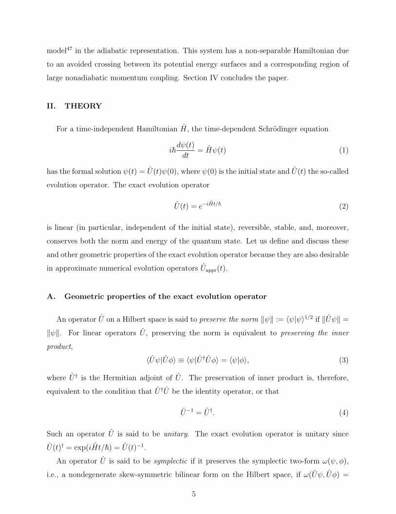
These conditions are visualized in Fig. 1. The exact evolution operator is stable but not

asymptotically stable because, due to norm conservation,

‖ψ(t)− φ(t)‖ = ‖ψ(0)− φ(0)‖. (12)

StableAsymptotically

stableUnstable

FIG. 1. Schematic representation of stability conditions in Euclidean space; the distance between

corresponding points on the two curves (e.g., the tips of the arrows) is analogous to a metric

‖ψ(t)− φ(t)‖ in the Hilbert space; the dotted lines represent ‖ψ(0)− φ(0)‖.

B. Loss of geometric properties by approximate methods

In approximate propagation methods, the state ψ(t+ ∆t) at time t+ ∆t, where ∆t is the

numerical time step, is obtained from the state ψ(t) at time t by applying an approximate

time evolution operator Uappr(∆t). This operator is

Uexpl(∆t) := 1− i

~∆t H (13)

in the explicit Euler method and

Uimpl(∆t) :=

(1 +

i

~∆t H

)−1

(14)

7

in the implicit Euler method. Both Euler methods are of the first order in the time step ∆t,

and both are neither unitary nor symplectic. Due to their lack of unitarity, the methods do

not conserve energy, even though their evolution operators commute with the Hamiltonian.

Neither method is symmetric; in fact, they are adjoints of each other. Hence, neither

method is time-reversible. The explicit Euler method is unstable with the distance between

two wavefunctions diverging,

‖ψexpl(t)− φexpl(t)‖ → ∞ as t→∞, (15)

whereas the implicit Euler method is asymptotically stable.

The second-order differencing method39–41 recovers symmetry by combining a forward

and backward steps of the explicit Euler method:

ψsod(t+ ∆t)− ψsod(t−∆t) = −2i

~∆tHψsod(t). (16)

The method can be also obtained directly from the time-dependent Schrodinger equation

by using a finite-difference approximation

dψ(t)

dt≈ ψ(t+ ∆t)− ψ(t−∆t)

2∆t. (17)

While it is almost as simple as the explicit Euler method to implement, the second order

differencing has a higher order of accuracy and, in contrast to the explicit Euler method,

it is symmetric, time-reversible, and at least conditionally stable, meaning that it remains

stable for sufficiently small time steps ∆t. The second order differencing does not conserve

the inner product, norm, energy, or symplectic two-form exactly. Yet, it conserves quantities

analogous to the inner product [see Eq. (A21)], norm,40,41 energy40,41 [see Eq. (A32)], and

symplectic two-form [see Eq. (A28)]. The corresponding exact quantities are conserved only

up to the fourth order in ∆t (see Propositions 5 and 6 of Appendix A).

The properties of the different methods are summarized in Table I; a more thorough

justification of these properties is provided in Appendix A. Although the explicit and implicit

Euler methods are not geometric, composing them in a specific way leads to arbitrary-

order integrators that preserve many important geometric properties of the exact solution.

Obviously, the compositions are applicable to systems with non-separable Hamiltonians just

like the elementary methods themselves.

8

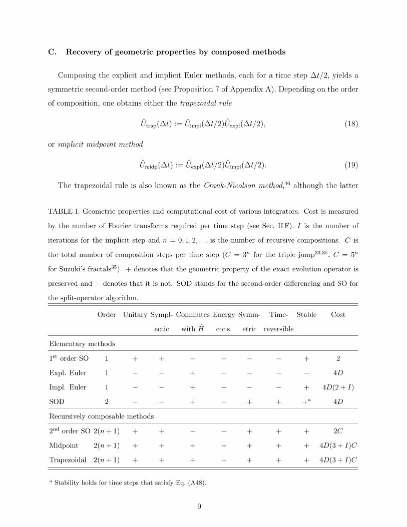
C. Recovery of geometric properties by composed methods

Composing the explicit and implicit Euler methods, each for a time step ∆t/2, yields a

symmetric second-order method (see Proposition 7 of Appendix A). Depending on the order

of composition, one obtains either the trapezoidal rule

Utrap(∆t) := Uimpl(∆t/2)Uexpl(∆t/2), (18)

or implicit midpoint method

Umidp(∆t) := Uexpl(∆t/2)Uimpl(∆t/2). (19)

The trapezoidal rule is also known as the Crank-Nicolson method,46 although the latter

TABLE I. Geometric properties and computational cost of various integrators. Cost is measured

by the number of Fourier transforms required per time step (see Sec. II F). I is the number of

iterations for the implicit step and n = 0, 1, 2, . . . is the number of recursive compositions. C is

the total number of composition steps per time step (C = 3n for the triple jump33,35, C = 5n

for Suzuki’s fractals35). + denotes that the geometric property of the exact evolution operator is

preserved and − denotes that it is not. SOD stands for the second-order differencing and SO for

the split-operator algorithm.

Order Unitary Sympl- Commutes Energy Symm- Time- Stable Cost

ectic with H cons. etric reversible

Elementary methods

1st order SO 1 + + − − − − + 2

Expl. Euler 1 − − + − − − − 4D

Impl. Euler 1 − − + − − − + 4D(2 + I)

SOD 2 − − + − + + +a 4D

Recursively composable methods

2nd order SO 2(n+ 1) + + − − + + + 2C

Midpoint 2(n+ 1) + + + + + + + 4D(3 + I)C

Trapezoidal 2(n+ 1) + + + + + + + 4D(3 + I)C

a Stability holds for time steps that satisfy Eq. (A48).

9

frequently implies a second-order finite-difference approximation to the spatial derivative in

the kinetic energy operator, whereas we use the dynamic Fourier method (see Sec. II E),

which has exponential convergence with grid density (see Appendix B).

Both the trapezoidal rule and implicit midpoint methods are Cayley transforms51 of

(i∆t/2~)H and, therefore, are unitary; in addition, both are second-order, symplectic, sym-

metric, time-reversible, and stable regardless of the size of the time step. Both methods

also commute with the Hamiltonian, are energy conserving, and can be further recursively

composed to obtain arbitrary-order methods (see Sec. II D). The summary of the properties

is given in Table I and a detailed justification provided in Appendix A.

It is necessary to stress that the geometric properties of the trapezoidal rule and implicit

midpoint method are only preserved if the implicit step, which involves solving a set of

linear equations, is executed exactly (or, in practice, to machine accuracy). We solved the

system of equations using the generalized minimal residual method,52–54 an iterative method

based on Arnoldi process.55,56 It was an appropriate choice since the matrix being inverted

was not positive-definite, symmetric, skew-symmetric, Hermitian, or skew-Hermitian, and

therefore neither conjugate gradient nor minimal residual method was applicable.54 The

initial guess for the implicit step was approximated with the explicit Euler method since for

small time steps, the solutions from the explicit and implicit Euler methods differ only by

(∆t/~)2H2|ψ(t)〉.

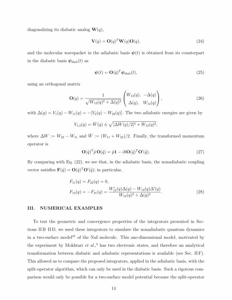
D. Symmetric composition schemes for symmetric methods

Recursively composing symmetric methods with appropriately chosen time steps leads

to symmetric integrators of arbitrary orders.27,33,35 More precisely, there exist a natural

number M and real numbers γn, n = 1, . . . ,M , called composition coefficients, satisfying∑M

n=1 γn = 1 and such that if Up(∆t) is any symmetric integrator of (necessarily even) order

p, then

Up+2(∆t) := Up(γM∆t) · · · Up(γ1∆t)

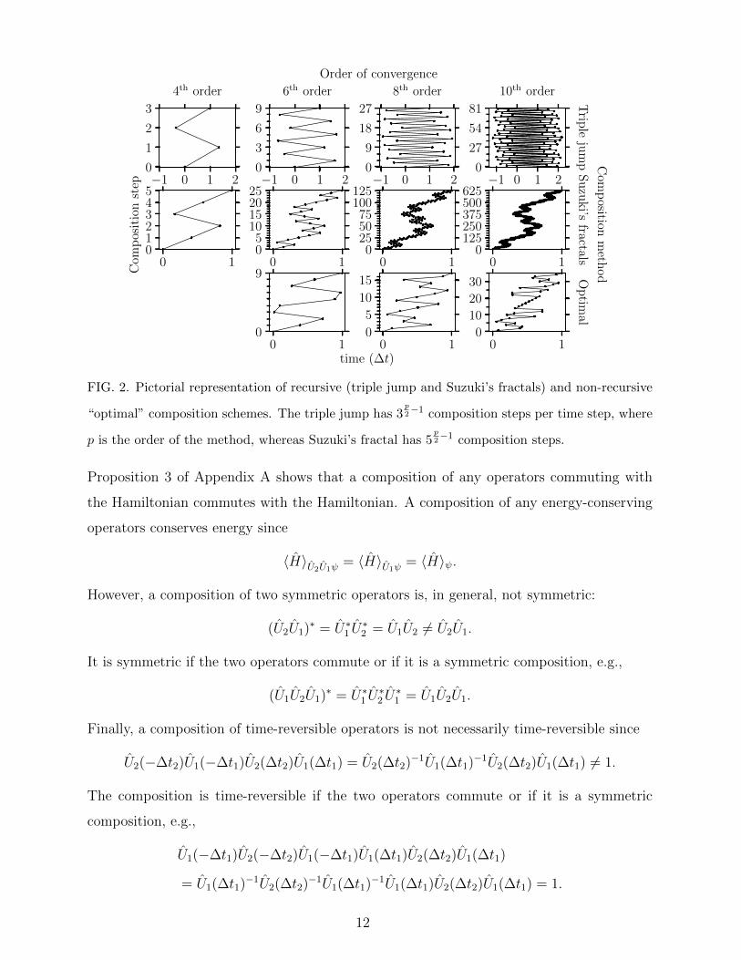
is a symmetric integrator of order p+2. The most common composition schemes (see Fig. 2)

are the triple jump33,35,57,58 with M = 3,

γ1 =1

2− 21/(p+1), γ2 = − 21/(p+1)

2− 21/(p+1), (20)

10

and Suzuki’s fractals35 with M = 5,

γ1 = γ2 =1

4− 41/(p+1), γ3 = − 41/(p+1)

4− 41/(p+1). (21)

The remaining coefficients are obtained from the relation γM+1−n = γn, which expresses that

both of these are symmetric compositions.

Because each triple jump is formed of three steps while each Suzuki’s fractal is composed of

five steps, the pth-order integrator obtained using Suzuki’s fractals has (5/3)p2−1 times more

composition steps than the one obtained from the same symmetric second-order method

using the triple jump. Therefore, the pth-order method obtained from Suzuki’s fractals takes

(5/3)p2−1 times longer to execute per time step ∆t than does the method of the same order

achieved through the triple jump. Yet, the leading order error coefficient of the pth-order

integrator based on Suzuki’s fractal is smaller because the magnitude of each composition

step is smaller in Suzuki’s fractal. Consequently, to achieve the same accuracy at a final time

t, larger time steps can be typically used for calculations using Suzuki’s fractals compared

to those based on the triple jump.

Non-recursive composition schemes, which require fewer composition steps and are also

more efficient, have been obtained for various specific orders. We will refer to these as “opti-

mal” schemes because they minimize the “magnitude” of composition steps. The magnitude

of composition steps can be defined as either maxn |γn| or∑M

n=1 |γn|. With either definition,

Suzuki’s fractal is the optimal fourth-order scheme. The optimal sixth- and eighth-order

schemes,59 found by Kahan and Li by minimizing maxn |γn|, have two more composition

steps (M = 9 and M = 17, respectively) than the minimum number possible for the re-

spective order; the optimal tenth-order scheme,60 obtained by Sofroniou and Spaletta by

minimizing∑M

n=1 |γn|, has four more (M = 35).

Theorem. All compositions of the trapezoidal rule or implicit midpoint method are

unitary, symplectic, stable, energy-conserving, and their evolution operators commute with

the Hamiltonian; all symmetric compositions are symmetric and therefore time-reversible.

Proof. We prove the theorem in much greater generality. Indeed, a composition of any

unitary operators U1 and U2 is unitary since

(U2U1)† = U †1 U†2 = U−1

1 U−12 = (U2U1)−1.

A composition of any symplectic operators is symplectic since

ω(U2U1ψ, U2U1φ) = ω(U1ψ, U1φ) = ω(ψ, φ).

11

−1 0 1 2

4th order

0

1

2

3

−1 0 1 2

6th order

0

3

6

9

−1 0 1 2

8th order

0

9

18

27

−1 0 1 2

10th order

0

27

54

81

Trip

leju

mp

0 1012345

0 105

10152025

0 10

255075

100125

0 10

125250375500625

Su

zuki’s

fractals

0 10

9

0 10

5

10

15

0 10

10

20

30

Op

timal

time (∆t)

Com

pos

itio

nst

epC

omp

ositionm

ethod

Order of convergence

FIG. 2. Pictorial representation of recursive (triple jump and Suzuki’s fractals) and non-recursive

“optimal” composition schemes. The triple jump has 3p2−1 composition steps per time step, where

p is the order of the method, whereas Suzuki’s fractal has 5p2−1 composition steps.

Proposition 3 of Appendix A shows that a composition of any operators commuting with

the Hamiltonian commutes with the Hamiltonian. A composition of any energy-conserving

operators conserves energy since

〈H〉U2U1ψ= 〈H〉U1ψ

= 〈H〉ψ.

However, a composition of two symmetric operators is, in general, not symmetric:

(U2U1)∗ = U∗1 U∗2 = U1U2 6= U2U1.

It is symmetric if the two operators commute or if it is a symmetric composition, e.g.,

(U1U2U1)∗ = U∗1 U∗2 U∗1 = U1U2U1.

Finally, a composition of time-reversible operators is not necessarily time-reversible since

U2(−∆t2)U1(−∆t1)U2(∆t2)U1(∆t1) = U2(∆t2)−1U1(∆t1)−1U2(∆t2)U1(∆t1) 6= 1.

The composition is time-reversible if the two operators commute or if it is a symmetric

composition, e.g.,

U1(−∆t1)U2(−∆t2)U1(−∆t1)U1(∆t1)U2(∆t2)U1(∆t1)

= U1(∆t1)−1U2(∆t2)−1U1(∆t1)−1U1(∆t1)U2(∆t2)U1(∆t1) = 1.

12

E. Dynamic Fourier method

To propagate the wavepacket using the explicit or implicit Euler method, or one of their

compositions (see Sec. II B–II D), only the action of the Hamiltonian operator H on ψ(t)

is required provided that the implicit steps are solved iteratively. The dynamic Fourier

method31,32,40,61 is an efficient approach to compute f(x)ψ(t), where f(x) is an arbitrary

function of x, which denotes either the nuclear position (q) or momentum (p) operator.

Each action of f(x) on ψ(t) is evaluated in the x-representation (in which x is diagonal)

by a simple multiplication, after Fourier-transforming ψ(t) to change the representation if

needed. On a grid of N points, f(x)ψ(t) is evaluated as f(xi)ψ(xi, t), 1 ≤ i ≤ N , where

ψ(x, t) is the wavepacket in the x-representation and xi are either the position or momentum

grid points.

F. Molecular Hamiltonian in the adiabatic basis

The molecular Hamiltonian in the adiabatic basis can be expressed as

H =1

2[p1− i~F(q)]† ·m−1 · [p1− i~F(q)] + V(q), (22)

where m is the diagonal D × D nuclear mass matrix, D the number of nuclear degrees of

freedom, V the diagonal S×S potential energy matrix, S the number of considered electronic

states, and F the nonadiabatic coupling vector (more precisely, a D-vector of S×S matrices).

In Eq. (22), the dot · denotes the matrix product in nuclear D-dimensional vector space,

the hatˆrepresents a nuclear operator, and the bold font indicates an electronic operator,

i.e., an S × S matrix. Using the dynamic Fourier method, each evaluation of the action of

H on a molecular wavepacket ψ(t), which now becomes an S-component vector of nuclear

wavepackets (one on each surface), involves 4D changes of the wavepacket’s representation.

In two-state models (i.e., for S = 2), it is possible to obtain H in the adiabatic represen-

tation analytically from the one in the diabatic representation,62–64

Hdiab =1

2pT ·m−1 · p1 + W(q), (23)

in which W(q) is the (real) diabatic potential energy matrix and in which the nonadia-

batic vector couplings vanish. The adiabatic potential energy matrix V(q) is obtained by

13

diagonalizing its diabatic analog W(q),

V(q) = O(q)TW(q)O(q), (24)

and the molecular wavepacket in the adiabatic basis ψ(t) is obtained from its counterpart

in the diabatic basis ψdiab(t) as

ψ(t) = O(q)Tψdiab(t), (25)

using an orthogonal matrix

O(q) =1√

W12(q)2 + ∆(q)2

W12(q), −∆(q)

∆(q), W12(q)

, (26)

with ∆(q) = V1(q)−W11(q) = −[V2(q)−W22(q)]. The two adiabatic energies are given by

V1,2(q) = W (q)±√

[∆W (q)/2]2 +W12(q)2,

where ∆W := W22 −W11 and W := (W11 + W22)/2. Finally, the transformed momentum

operator is

O(q)T pO(q) = p1− i~O(q)TO′(q). (27)

By comparing with Eq. (22), we see that, in the adiabatic basis, the nonadiabatic coupling

vector satisfies F(q) = O(q)TO′(q); in particular,

F11(q) = F22(q) = 0,

F12(q) = −F21(q) =W ′

12(q)∆(q)−W12(q)∆′(q)

W12(q)2 + ∆(q)2. (28)

III. NUMERICAL EXAMPLES

To test the geometric and convergence properties of the integrators presented in Sec-

tions II B–II D, we used these integrators to simulate the nonadiabatic quantum dynamics

in a two-surface model47 of the NaI molecule. This one-dimensional model, motivated by

the experiment by Mokhtari et al.,3 has two electronic states, and therefore an analytical

transformation between diabatic and adiabatic representations is available (see Sec. II F).

This allowed us to compare the proposed integrators, applied in the adiabatic basis, with the

split-operator algorithm, which can only be used in the diabatic basis. Such a rigorous com-

parison would only be possible for a two-surface model potential because the split-operator

14

algorithm requires the diabatization of the Hamiltonian formulated in the adiabatic repre-

sentation and this cannot be done exactly for higher-dimensional ab initio potential energy

surfaces with more electronic states.

Before the electronic excitation, the NaI molecule was assumed to be in the ground

vibrational eigenstate of a harmonic fit to the ground-state potential energy surface at

the equilibrium geometry. This vibrational wavepacket was then lifted to the excited-state

surface, in order to obtain an initial Gaussian wavepacket (q0 = 4.9889 a.u., p0 = 0 a.u., σ0 =

0.110436 a.u.) for the nonadiabatic dynamics. This use of the sudden approximation assumes

an impulsive excitation, i.e., the simultaneous validity of the time-dependent perturbation

theory and Condon and ultrashort pulse approximations during the excitation process. After

that, the nonadiabatic dynamics was performed by solving the time-dependent Schrodinger

equation using the dynamic Fourier method (see Sec. II E) on a uniform grid with 2048

points between q = 3.8 a.u. and q = 47.0 a.u.; Appendix B shows wavepacket represented

on such a grid is converged for the duration of the dynamics. A long-enough propagation

time, tf = 10500 a.u., was chosen so that the wavepacket traverses the avoided crossing and

simultaneously witnesses the change of the nature of the excited adiabatic state from covalent

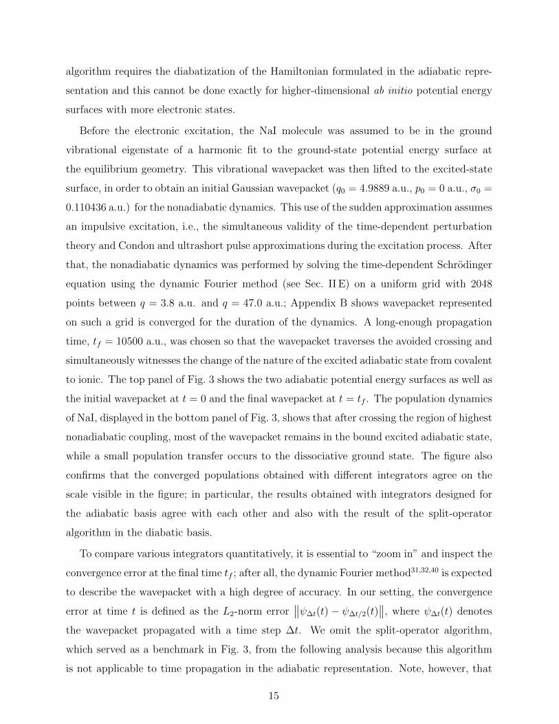
to ionic. The top panel of Fig. 3 shows the two adiabatic potential energy surfaces as well as

the initial wavepacket at t = 0 and the final wavepacket at t = tf . The population dynamics

of NaI, displayed in the bottom panel of Fig. 3, shows that after crossing the region of highest

nonadiabatic coupling, most of the wavepacket remains in the bound excited adiabatic state,

while a small population transfer occurs to the dissociative ground state. The figure also

confirms that the converged populations obtained with different integrators agree on the

scale visible in the figure; in particular, the results obtained with integrators designed for

the adiabatic basis agree with each other and also with the result of the split-operator

algorithm in the diabatic basis.

To compare various integrators quantitatively, it is essential to “zoom in” and inspect the

convergence error at the final time tf ; after all, the dynamic Fourier method31,32,40 is expected

to describe the wavepacket with a high degree of accuracy. In our setting, the convergence

error at time t is defined as the L2-norm error∥∥ψ∆t(t)− ψ∆t/2(t)

∥∥, where ψ∆t(t) denotes

the wavepacket propagated with a time step ∆t. We omit the split-operator algorithm,

which served as a benchmark in Fig. 3, from the following analysis because this algorithm

is not applicable to time propagation in the adiabatic representation. Note, however, that

15

0.951.0

P2

SOD

Trapezoidal

Midpoint

Split-operator

0 2500 5000 7500 10000

t (a.u.)

0.00.05 P1

10 20

q (a.u.)

0

1

E(a

.u.)

or|ψ

(q,t

)|/3 V11

V22

|F12|ψ1(q, tf )

ψ2(q, 0)

ψ2(q, tf )

Pj

FIG. 3. Nonadiabatic dynamics of NaI. Top: Adiabatic potential energy surfaces with the initial

and final nuclear wavepacket components in the ground and excited adiabatic electronic states

[Because the initial molecular wavepacket was in the excited state, its component ψ1(q, t = 0) ≡

0 is not shown.]. Bottom: Ground- and excited-state populations of NaI computed with four

different second-order methods: SOD stands for the second-order differencing. The populations

were propagated with a time step ∆t = 0.01 a.u., i.e., much more frequently than the markers

suggest. The small time step guaranteed wavepacket convergence errors below ≈ 10−6 in all

methods.

for separable Hamiltonians, such as the nonadiabatic Hamiltonian in the diabatic basis, the

split-operator algorithms are more efficient than the present integrators of the corresponding

order (see Table I and Paper II).

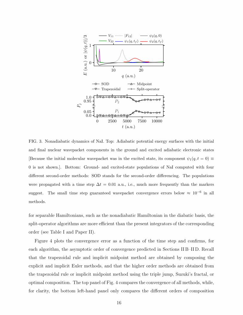
Figure 4 plots the convergence error as a function of the time step and confirms, for

each algorithm, the asymptotic order of convergence predicted in Sections II B–II D. Recall

that the trapezoidal rule and implicit midpoint method are obtained by composing the

explicit and implicit Euler methods, and that the higher order methods are obtained from

the trapezoidal rule or implicit midpoint method using the triple jump, Suzuki’s fractal, or

optimal composition. The top panel of Fig. 4 compares the convergence of all methods, while,

for clarity, the bottom left-hand panel only compares the different orders of composition

16

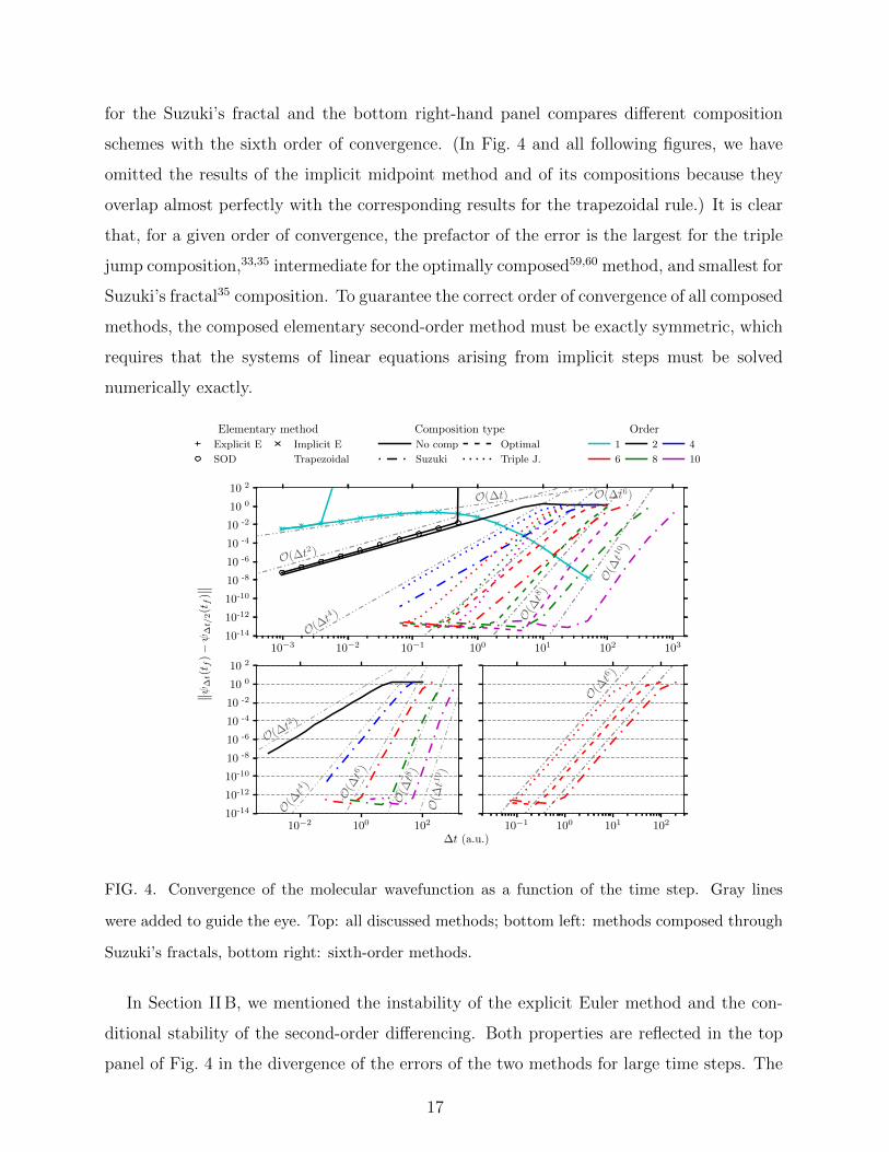
for the Suzuki’s fractal and the bottom right-hand panel compares different composition

schemes with the sixth order of convergence. (In Fig. 4 and all following figures, we have

omitted the results of the implicit midpoint method and of its compositions because they

overlap almost perfectly with the corresponding results for the trapezoidal rule.) It is clear

that, for a given order of convergence, the prefactor of the error is the largest for the triple

jump composition,33,35 intermediate for the optimally composed59,60 method, and smallest for

Suzuki’s fractal35 composition. To guarantee the correct order of convergence of all composed

methods, the composed elementary second-order method must be exactly symmetric, which

requires that the systems of linear equations arising from implicit steps must be solved

numerically exactly.

10−3 10−2 10−1 100 101 102 10310-14

10-12

10-10

10 -8

10 -6

10 -4

10 -2

10 0

10 2

O(∆t)

O(∆t2 )

O(∆t4 )

O(∆t6)

O(∆t

8 )

O(∆t1

0 )

10−1 100 101 102

O(∆t6 )

10−2 100 10210-14

10-12

10-10

10 -8

10 -6

10 -4

10 -2

10 0

10 2

O(∆t2 )

O(∆t

4 )

O(∆t

6 )

O(∆t8

)

O(∆t1

0 )

∥ ∥ ψ∆t(tf)−ψ

∆t/

2(tf)∥ ∥

∆t (a.u.)

Order

1

6

2

8

4

10

Composition type

No comp

Suzuki

Optimal

Triple J.

Elementary method

Explicit E

SOD

Implicit E

Trapezoidal

FIG. 4. Convergence of the molecular wavefunction as a function of the time step. Gray lines

were added to guide the eye. Top: all discussed methods; bottom left: methods composed through

Suzuki’s fractals, bottom right: sixth-order methods.

In Section II B, we mentioned the instability of the explicit Euler method and the con-

ditional stability of the second-order differencing. Both properties are reflected in the top

panel of Fig. 4 in the divergence of the errors of the two methods for large time steps. The

17

critical time step for the second-order differencing is ∆t ≈ 0.5 a.u., whereas the explicit Euler

method is unstable regardless of ∆t but the effect of instability is more visible for larger time

steps. In contrast, the trapezoidal rule, implicit midpoint method, and their compositions

are stable, but implicit, and, therefore, require the solution of systems of linear equations.

These methods could not be used beyond a certain time step (maxn |γn|∆t ≈ 100 a.u. for

both the trapezoidal rule and implicit midpoint method) because the iterative generalized

minimal residual algorithm did not converge for very large ∆t.

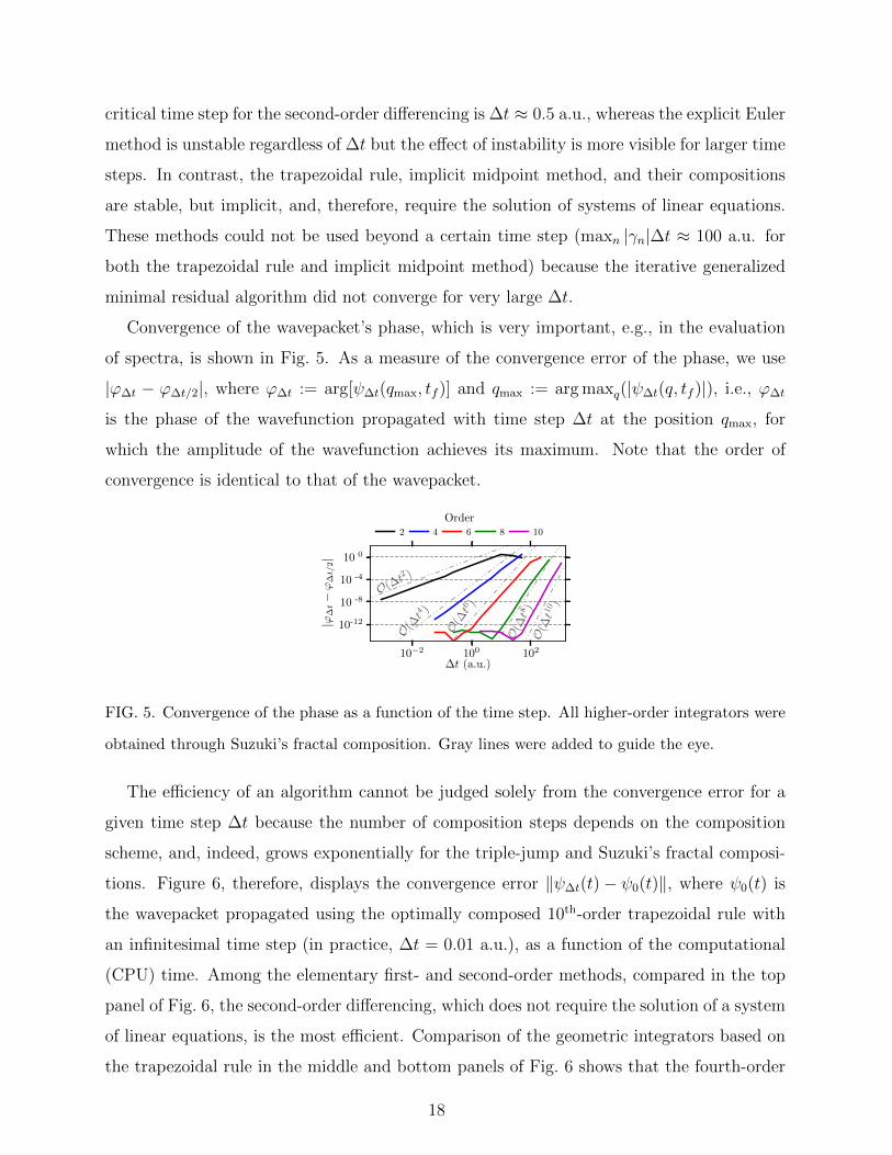
Convergence of the wavepacket’s phase, which is very important, e.g., in the evaluation

of spectra, is shown in Fig. 5. As a measure of the convergence error of the phase, we use

|ϕ∆t − ϕ∆t/2|, where ϕ∆t := arg[ψ∆t(qmax, tf )] and qmax := arg maxq(|ψ∆t(q, tf )|), i.e., ϕ∆t

is the phase of the wavefunction propagated with time step ∆t at the position qmax, for

which the amplitude of the wavefunction achieves its maximum. Note that the order of

convergence is identical to that of the wavepacket.

10−2 100 102

10-12

10 -8

10 -4

10 0

O(∆t2 )

O(∆t4 )

O(∆t

6 )

O(∆t8

)O(

∆t1

0 )

|ϕ∆t−ϕ

∆t/

2|

∆t (a.u.)

Order2 4 6 8 10

FIG. 5. Convergence of the phase as a function of the time step. All higher-order integrators were

obtained through Suzuki’s fractal composition. Gray lines were added to guide the eye.

The efficiency of an algorithm cannot be judged solely from the convergence error for a

given time step ∆t because the number of composition steps depends on the composition

scheme, and, indeed, grows exponentially for the triple-jump and Suzuki’s fractal composi-

tions. Figure 6, therefore, displays the convergence error ‖ψ∆t(t)− ψ0(t)‖, where ψ0(t) is

the wavepacket propagated using the optimally composed 10th-order trapezoidal rule with

an infinitesimal time step (in practice, ∆t = 0.01 a.u.), as a function of the computational

(CPU) time. Among the elementary first- and second-order methods, compared in the top

panel of Fig. 6, the second-order differencing, which does not require the solution of a system

of linear equations, is the most efficient. Comparison of the geometric integrators based on

the trapezoidal rule in the middle and bottom panels of Fig. 6 shows that the fourth-order

18

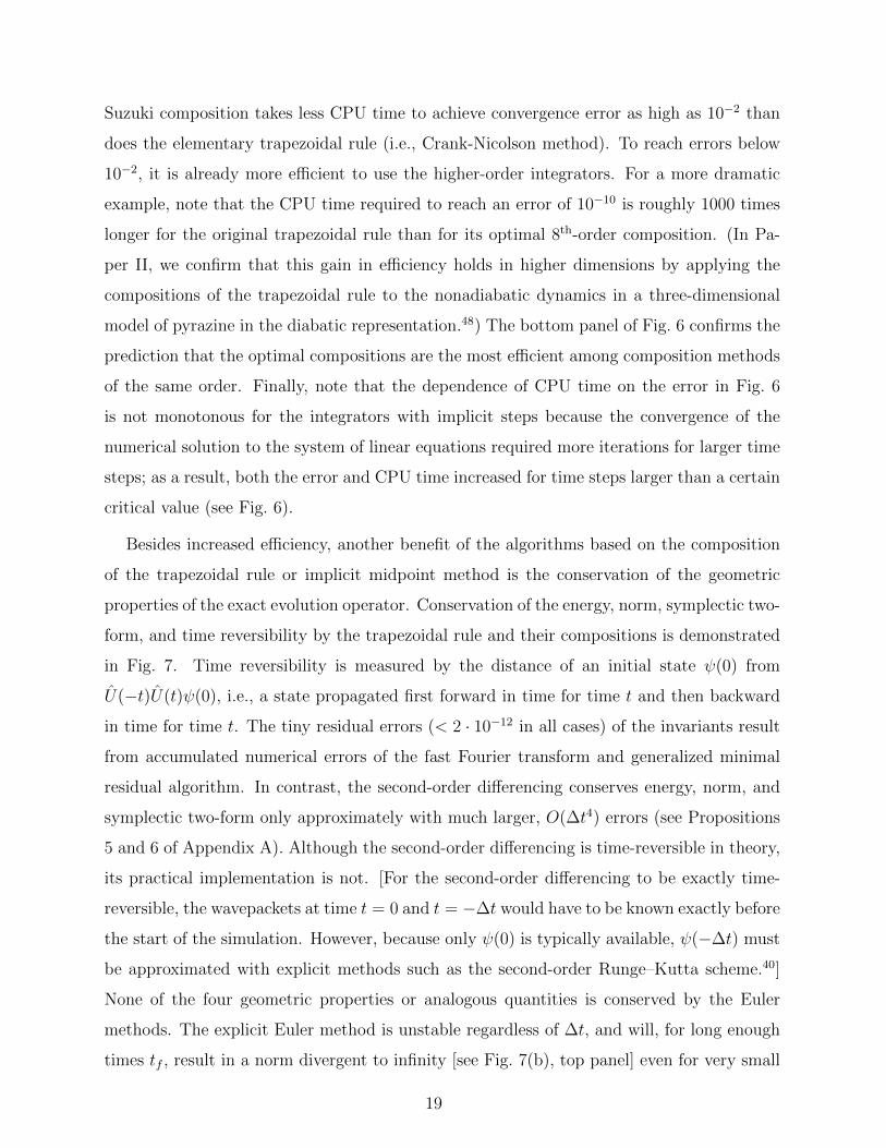
Suzuki composition takes less CPU time to achieve convergence error as high as 10−2 than

does the elementary trapezoidal rule (i.e., Crank-Nicolson method). To reach errors below

10−2, it is already more efficient to use the higher-order integrators. For a more dramatic

example, note that the CPU time required to reach an error of 10−10 is roughly 1000 times

longer for the original trapezoidal rule than for its optimal 8th-order composition. (In Pa-

per II, we confirm that this gain in efficiency holds in higher dimensions by applying the

compositions of the trapezoidal rule to the nonadiabatic dynamics in a three-dimensional

model of pyrazine in the diabatic representation.48) The bottom panel of Fig. 6 confirms the

prediction that the optimal compositions are the most efficient among composition methods

of the same order. Finally, note that the dependence of CPU time on the error in Fig. 6

is not monotonous for the integrators with implicit steps because the convergence of the

numerical solution to the system of linear equations required more iterations for larger time

steps; as a result, both the error and CPU time increased for time steps larger than a certain

critical value (see Fig. 6).

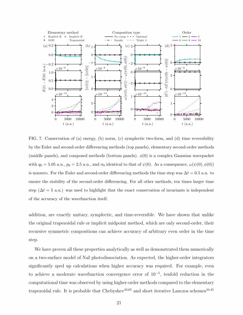
Besides increased efficiency, another benefit of the algorithms based on the composition

of the trapezoidal rule or implicit midpoint method is the conservation of the geometric

properties of the exact evolution operator. Conservation of the energy, norm, symplectic two-

form, and time reversibility by the trapezoidal rule and their compositions is demonstrated

in Fig. 7. Time reversibility is measured by the distance of an initial state ψ(0) from

U(−t)U(t)ψ(0), i.e., a state propagated first forward in time for time t and then backward

in time for time t. The tiny residual errors (< 2 · 10−12 in all cases) of the invariants result

from accumulated numerical errors of the fast Fourier transform and generalized minimal

residual algorithm. In contrast, the second-order differencing conserves energy, norm, and

symplectic two-form only approximately with much larger, O(∆t4) errors (see Propositions

5 and 6 of Appendix A). Although the second-order differencing is time-reversible in theory,

its practical implementation is not. [For the second-order differencing to be exactly time-

reversible, the wavepackets at time t = 0 and t = −∆t would have to be known exactly before

the start of the simulation. However, because only ψ(0) is typically available, ψ(−∆t) must

be approximated with explicit methods such as the second-order Runge–Kutta scheme.40]

None of the four geometric properties or analogous quantities is conserved by the Euler

methods. The explicit Euler method is unstable regardless of ∆t, and will, for long enough

times tf , result in a norm divergent to infinity [see Fig. 7(b), top panel] even for very small

19

∆t, implying that also the wavefunction will have an error increasing beyond any bound. As

for the implicit Euler method, its error of the norm converges to −1 because ‖ψimpl(t)‖ → 0

as t→∞ [see Fig. 7(b), top panel].

IV. CONCLUSION

We have described geometric integrators for nonadiabatic quantum dynamics in the adi-

abatic representation, in which the popular split-operator algorithms cannot be used due

to nonseparability of the Hamiltonian into a kinetic and potential terms. The proposed

methods are based on the symmetric composition of the trapezoidal rule or implicit mid-

point method, and as a result, are symmetric, stable, conserve the energy exactly and, in

10 -8

10 -4

10 0

101 102 103 104 105 106

10-12

10 -8

10 -4

10 0

103 104

CPU time (s)

10-12

10-10

10 -8

10 -6

10 -4‖ψ∆t(tf)−ψ

0(tf)‖

Order1

6

2

8

4

10

Composition typeNo comp

Suzuki

Optimal

Triple J.

Elementary methodExplicit E

SOD

Implicit E

Trapezoidal

FIG. 6. Efficiency of various methods shown using the dependence of the convergence error on the

computational (CPU) time. Results of the elementary trapezoidal rule were extrapolated using the

line of best fit to highlight the speedup achieved with higher-order compositions. Top: elementary

methods; middle: trapezoidal rule and its compositions; bottom: detail of the middle panel.

20

−0.2

0.0

0.2(a)

0.0

0.5

1.0×10−9

0 5000 10000

t (a.u.)

0

2

4

×10−15

−1

0

1(b)

0

1

×10−8

0 5000 10000

t (a.u.)

0

5

×10−14

−2

0

2(c)

−2

0×10−9

0 5000 10000

t (a.u.)

0

1×10−13

0

5(d)

0

2

×10−2

0 5000 10000

t (a.u.)

0

1

×10−12

E(t

)−E

(0)

(a.u

.)

‖ψ(t

)‖−‖ψ

(0)‖

ω(ψ

(t),φ

(t))−ω

(ψ(0

),φ

(0))

‖U(−t)U

(t)ψ

(0)−ψ

(0)‖

Order1

6

2

8

4

10

Composition typeNo comp

Suzuki

Optimal

Triple J.

Elementary methodExplicit E

SOD

Implicit E

Trapezoidal

FIG. 7. Conservation of (a) energy, (b) norm, (c) symplectic two-form, and (d) time reversibility

by the Euler and second-order differencing methods (top panels), elementary second-order methods

(middle panels), and composed methods (bottom panels). φ(0) is a complex Gaussian wavepacket

with q0 = 5.05 a.u., p0 = 2.5 a.u., and σ0 identical to that of ψ(0). As a consequence, ω(ψ(0), φ(0))

is nonzero. For the Euler and second-order differencing methods the time step was ∆t = 0.5 a.u. to

ensure the stability of the second-order differencing. For all other methods, ten times larger time

step (∆t = 5 a.u.) was used to highlight that the exact conservation of invariants is independent

of the accuracy of the wavefunction itself.

addition, are exactly unitary, symplectic, and time-reversible. We have shown that unlike

the original trapezoidal rule or implicit midpoint method, which are only second-order, their

recursive symmetric compositions can achieve accuracy of arbitrary even order in the time

step.

We have proven all these properties analytically as well as demonstrated them numerically

on a two-surface model of NaI photodissociation. As expected, the higher-order integrators

significantly sped up calculations when higher accuracy was required. For example, even

to achieve a moderate wavefunction convergence error of 10−5, tenfold reduction in the

computational time was observed by using higher-order methods compared to the elementary

trapezoidal rule. It is probable that Chebyshev43,65 and short iterative Lanczos schemes44,45

21

would be more efficient in this and other typical systems, but these methods do not conserve

exactly all the invariants conserved by the described geometric integrators.

Finally, we hope that the ability to run “geometric” quantum molecular dynamics in

the adiabatic representation will be useful especially in conjunction with potential energy

surfaces obtained from ab initio electronic structure calculations because this will avoid the

tedious diabatization process necessary for the applicability of the split-operator algorithm.

The authors acknowledge the financial support from the European Research Council

(ERC) under the European Union’s Horizon 2020 research and innovation programme (grant

agreement No. 683069 – MOLEQULE), and thank Nikolay Golubev and Rob Parrish for

useful discussions.

Appendix A: Geometric properties of various integrators

To shorten formulas, we set ~ = 1 and denote the increment ∆t with ε throughout the

Appendix. The ~ can be reintroduced by replacing each occurrence of t with t/~ (and ε

with ε/~). To analyze geometric properties of various integrators, we will use the following

operator identities:

Proposition 1. Let A and B be invertible operators on a Hilbert space, and let A†

and B† their Hermitian adjoints. Then both A† and AB are invertible, and the following

identities hold:

(A†)−1 = (A−1)†, (A1)

(AB)−1 = B−1A−1, (A2)

(AB)† = B†A†, (A3)

(A†)† = (A−1)−1 = A. (A4)

The first property expresses the compatibility of the inverse and Hermitian adjoint op-

erations, while the last three properties express that these two operations are involutive

antiautomorphisms on the group of invertible operators. All four properties are easy to

prove in finite-dimensional spaces;66 the proofs for infinite-dimensional spaces can be found

in textbooks on advanced linear algebra or functional analysis.67

Proposition 2. Let A and B be commuting operators on a vector space, i.e., [A, B] :=

AB − BA = 0. If A is invertible, then [A−1, B] = 0. If both A and B are invertible, then

22

[A−1, B−1] = 0.

The first statement follows from the sequence of identities

A−1B = A−1BAA−1 = A−1ABA−1 = BA−1.

The second statement follows from the first by applying it twice, the second time for A := B

and B := A−1, or directly from

A−1B−1 = (BA)−1 = (AB)−1 = B−1A−1

by using property (A2).

Proposition 3. Let A, B, and H be operators on a vector space. If [H, A] = [H, B] = 0,

then [H, AB] = 0.

This follows immediately from the identity [H, AB] = A[H, B] + [H, A]B.

1. Local error

The local error of an approximate evolution operator, defined as Uappr(ε) − U(ε), is ob-

tained by comparing the Taylor expansion of Uappr(ε) with the Taylor expansion of the exact

evolution operator:

U(ε) = e−iεH = 1− iεH − 1

2!(εH)2 +

i

3!(εH)3 +O(ε4). (A5)

If the local error is O(εn+1), the method is said to be of order n because the global error for

a finite time t = Nε is O(εn).

For the explicit Euler method, the Taylor expansion is identical to the evolution operator

(13) itself, and therefore the leading order local error is (εH)2/2. The Taylor expansion of

the implicit Euler method (14) is the Neumann series68

Uimpl(ε) = (1 + iεH)−1 = 1− iεH + (iεH)2 − (iεH)3 +O(ε4); (A6)

the leading order local error is −(εH)2/2.

The Taylor expansions of the trapezoidal rule and implicit midpoint method are obtained

by composing Eqs. (13) and (A6) with time steps ε/2:

Utrap(ε) = Umidp(ε) = 1− iεH − 1

2(εH)2 +

i

4(εH)3 +O(ε4); (A7)

23

the leading order local error of both methods is i(εH)3/12.

Finally, the local error of the second-order differencing method is

− i

3(εH)3 +O(ε4), (A8)

which is found by Taylor expanding ψsod(t− ε), assumed to be exact, in Eq. (16) to obtain

ψsod(t+ ε) =

(1− iεH − 1

2!(εH)2 − i

3!(εH)3 +O(ε4)

)ψsod(t) (A9)

and

Usod = 1− iεH − 1

2!(εH)2 − i

3!(εH)3 +O(ε4). (A10)

Subtracting Eq. (A5) from Eq. (A10) gives the local error (A8).

2. Unitarity

Neither Euler method is unitary because

Uexpl(ε)†Uexpl(ε) = (1 + iεH)(1− iεH)

= 1 + ε2H2 (A11)

and

Uimpl(ε)†Uimpl(ε) = (1− iεH)−1(1 + iεH)−1

=(

(1 + iεH)(1− iεH))−1

= (1 + ε2H2)−1

= 1− ε2H2 +O(ε4). (A12)

In contrast, both the trapezoidal rule and implicit midpoint methods are unitary because

Utrap(ε)†Utrap(ε) =

(1 +

iε

2H

)(1− iε

2H

)−1(1 +

iε

2H

)−1(1− iε

2H

)

=

(1 +

iε

2H

)(1 +

iε

2H

)−1(1− iε

2H

)−1(1− iε

2H

)

= 1 · 1 = 1, (A13)

24

(Proposition 1 was used in the first and Proposition 2 in the second line) and because

Umidp(ε)†Umidp(ε) =

(1− iε

2H

)−1(1 +

iε

2H

)(1− iε

2H

)(1 +

iε

2H

)−1

=

(1− iε

2H

)−1(1− iε

2H

)(1 + i

ε

2H)(

1 +iε

2H

)−1

= 1 · 1 = 1 (A14)

(Proposition 1 was used in the first line).

The analysis of its geometric properties is simplified if the second-order differencing is

represented by a 2× 2 propagation matrix

Usod(ε) :=

1− (2εH)2, −2iεH

−2iεH, 1

(A15)

acting on a vector of ψ at two different times:41

ψsod(t+ ε)

ψsod(t)

= Usod(ε)

ψsod(t− ε)ψsod(t− 2ε)

. (A16)

Comparing the Hermitian conjugate Usod(ε)† of Usod(ε) with its inverse,

Usod(ε)−1 =

1, 2iεH

2iεH, 1− (2εH)2

, (A17)

found using det Usod(ε) = 1, shows that the second-order differencing is not unitary.

When U(ε) is not unitary, we can obtain the time dependence of the norm from

‖ψ(t+ ε)‖2 = 〈ψ(t)|U(ε)†U(ε)|ψ(t)〉. (A18)

For the explicit and implicit Euler methods, we find that

‖ψexpl(t+ ε)‖2 = ‖ψexpl(t)‖2 + ε2〈H2〉ψexpl(t), (A19)

‖ψimpl(t+ ε)‖2 = ‖ψimpl(t)‖2 − ε2〈H2〉ψimpl(t) +O(ε3), (A20)

where 〈A〉ψ := 〈ψ|A|ψ〉 denotes the expectation value of operator A in state ψ.

Although the second-order differencing is not unitary, a conserved quantity analogous to

the inner product exists:

25

Proposition 4. The second-order differencing conserves the quantity

(〈ψsod(t)|φsod(t− ε)〉+ 〈ψsod(t− ε)|φsod(t)〉)/2. (A21)

The proof starts by projecting 〈φsod(t)| on Eq. (16), which yields

〈φsod(t)|ψsod(t+ ε)〉 = 〈φsod(t)|ψsod(t− ε)〉 − 2iε〈φsod(t)|H|ψsod(t)〉. (A22)

Adding the complex conjugate of Eq. (A22) to the analogue of Eq. (A22), in which ψ and

φ are exchanged, gives

〈ψsod(t)|φsod(t+ ε)〉+ 〈ψsod(t+ ε)|φsod(t)〉

= 〈ψsod(t)|φsod(t− ε)〉+ 〈ψsod(t− ε)|φsod(t)〉,

completing the proof. As an immediate corollary, obtained by taking φ = ψ, the second-

order differencing conserves the quantity Re〈ψsod(t)|ψsod(t− ε)〉, which is an analogue of the

norm.40

Proposition 5. The global error of the inner product between two quantum states propa-

gated by the second-order differencing is fourth-order in the time step, i.e., 〈ψsod(tf )|φsod(tf )〉−〈ψ(0)|φ(0)〉 = O(ε4).

Assuming that the wavepackets at t = −ε are known exactly, Proposition 4 implies

〈ψsod(tf + ε)|φsod(tf )〉+ 〈ψsod(tf )|φsod(tf + ε)〉 = 〈ψ(0)|φ(−ε)〉+ 〈ψ(−ε)|φ(0)〉. (A23)

By Taylor expanding ψ(−ε) and φ(−ε), and using Eq. (A9), we obtain

〈ψsod(tf )|φsod(tf )〉 −ε2

2〈ψsod(tf )|H2|φsod(tf )〉 = 〈ψ(0)|φ(0)〉 − ε2

2〈ψ(0)|H2|φ(0)〉+O(ε4).

Rearranging the two sides gives

〈ψsod(tf )|φsod(tf )〉 − 〈ψ(0)|φ(0)〉 =ε2

2

[〈ψsod(tf )|H2|φsod(tf )〉 − 〈ψ(0)|H2|φ(0)〉

]+O(ε4).

(A24)

The global error of the second-order differencing method is second-order in the time step

and, therefore,

ψsod(tf ) = ψ(tf ) +O(ε2), (A25)

φsod(tf ) = φ(tf ) +O(ε2).

Noting that under exact evolution, 〈ψ(tf )|H2|φ(tf )〉 = 〈ψ(0)|H2|φ(0)〉, we obtain Proposi-

tion 5 by substituting Eq. (A25) into Eq. (A24).

26

3. Symplecticity

Using a shorthand notation ωappr|t := ω(ψappr(t), φappr(t)) and expressions Uappr(ε)†Uappr(ε)

from Appendix A 2 for the two Euler methods gives

ωexpl|t+ε = ωexpl|t − 2~ε2Im〈ψexpl(t)|H2|φexpl(t)〉 (A26)

ωimpl|t+ε = ωimpl|t + 2~ε2Im〈ψimpl(t)|H2|φimpl(t)〉+O(ε3), (A27)

showing that neither first-order method is symplectic. In contrast, both the trapezoidal rule

and implicit midpoint methods are symplectic because they are unitary.

Finally, the second-order differencing is strictly not symplectic, but Proposition 4 implies

that the quantity

− ~Im[〈ψsod(t)|φsod(t+ ε)〉+ 〈ψsod(t+ ε)|φsod(t)〉], (A28)

analogous to the symplectic two-form, is conserved. In fact, Proposition 5 shows that the

global error of the symplectic two-form is O(ε4).

4. Commutation of the evolution operator with the Hamiltonian

Evolution operators of both Euler methods commute with the Hamiltonian:

[H, Uexpl(ε)] = [H, 1− iεH] = 0, (A29)

[H, Uimpl(ε)] = [H, (1 + iεH)−1] = 0, (A30)

where in Eq. (A30), Proposition 2 was used. Applying Proposition 3 to A = Uexpl(ε/2)

and B = Uimpl(ε/2) (or vice versa) then shows that the evolution operators of both the

trapezoidal rule and implicit midpoint methods commute with the Hamiltonian. As for the

second-order differencing, all entries in Usod are polynomials in H and hence commute with

H; as a result, [H, Usod] = 0 as well.

5. Energy conservation

Neither Euler method is unitary and hence neither conserves the energy. In contrast, both

the trapezoidal rule and implicit midpoint methods conserve energy because their evolution

operators are unitary and commute with the Hamiltonian.

27

The second-order differencing does not conserve energy exactly but a conserved quantity

analogous to the energy has been defined:41 Applying 〈ψsod(t)|H to Eq. (16) gives

〈ψsod(t)|H|ψsod(t+ ε)〉 = −2iε〈H2〉ψsod(t) + 〈ψsod(t)|H|ψsod(t− ε)〉. (A31)

Because 〈H2〉ψsod(t) is real, taking the real part of Eq. (A31) shows that

Re〈ψsod(t)|H|ψsod(t+ ε)〉 (A32)

is conserved.

Proposition 6. The global error of the expectation value of energy of the quantum state

propagated by the second-order differencing is fourth-order in the time step, i.e., 〈H〉ψsod(tf )−〈H〉ψ(0) = O(ε4).

From Eq. (A32),

Re〈ψsod(tf )|H|ψsod(tf + ε)〉 = Re〈ψ(−ε)|H|ψ(0)〉. (A33)

Assuming, as in the proof of Proposition 5, that ψ(−ε) is known exactly, by Taylor expanding

ψ(−ε) and using Eq. (A9), we obtain

〈H〉ψsod(tf ) − 〈H〉ψ(0) =ε2

2

[〈H3〉ψsod(tf ) − 〈H3〉ψ(0)

]+O(ε4). (A34)

Invoking Eq. (A25) and identity 〈H3〉ψ(tf ) = 〈H3〉ψ(0) completes the proof of Proposition 6.

6. Symmetry

Proposition 7. The adjoint of an evolution operator has the following properties:

(U(ε)∗)∗ = U(ε), (A35)

(U1(ε)U2(ε))∗ = U2(ε)∗U1(ε)∗, (A36)

U(ε)U(ε)∗ is symmetric. (A37)

The first and second properties mean, respectively, that the adjoint operation ∗ is an

involution and an antiautomorphism on the group of invertible operators, while the last

property provides the simplest recipe for constructing a symmetric method—by composing

a general method with its adjoint, with both composition coefficients of 1/2. All three

properties follow directly from the definition: the first because (U(ε)∗)∗ = (U(−ε)∗)−1 =

28

(U(ε)−1)−1, the second because (U1(ε)U2(ε))∗ = (U1(−ε)U2(−ε))−1 = U2(−ε)−1U1(−ε)−1,

and the third by applying Eq. (A36) to the product of U and U∗, and using Eq. (A35).

The explicit and implicit Euler methods are adjoints of each other, which follows from

Uexpl(−ε)−1 = (1 + iHε)−1 = Uimpl(ε) (A38)

and Eq. (A35). Therefore, neither method is symmetric. In contrast, the trapezoidal rule

and implicit midpoint methods are both symmetric, which follows from Eq. (A37) applied

to the composition of the explicit and implicit Euler methods with composition coefficients

1/2.

Taking the inverse of Usod(−ε) gives

Usod(−ε)−1 =

1, −2iεH

−2iεH, 1− (2εH)2

=

0 1

1 0

Usod(ε)

0 1

1 0

, (A39)

implying that the second order differencing is symmetric if the sequence of wavefunctions is

reversed when taking the inverse.

7. Time reversibility

For an elementary time step ε, time reversibility is a direct consequence of the symmetry

of the operator: if the operator is symmetric, i.e., if U(−ε)−1 = U(ε), then a forward

propagation is exactly cancelled by the immediately following backward propagation:

U(−ε)U(ε) = U(−ε)U(−ε)−1 = 1. (A40)

This argument is easily extended, by induction, to a forward propagation forN steps followed

by a backward propagation for N steps:

U(−ε)N U(ε)N = 1.

As a result, the Euler methods are not time-reversible, whereas the trapezoidal rule, implicit

midpoint, and second-order differencing methods are.

29

8. Stability

The explicit Euler method is unstable because, using Eq. (A19),

‖ψ(t+ ε)− φ(t+ ε)‖2 = ‖ψ(t)− φ(t)‖2 + ε2〈H2〉ψ(t)−φ(t)

≥ (1 + ε2E2min)‖ψ(t)− φ(t)‖2, (A41)

as long as H has no eigenvalue in the finite interval (−Emin, Emin); composing the above

inequality N times shows that

‖ψ(Nε)− φ(Nε)‖2 ≥ (1 + ε2E2min)N‖ψ(0)− φ(0)‖2 →∞ (A42)

as N →∞ for ψ(0) 6= φ(0).

Asymptotic stability of the implicit Euler method follows, using Eq. (A20), from an

analogous inequality

‖ψ(t)− φ(t)‖2 = ‖ψ(t+ ε)− φ(t+ ε)‖2 + ε2〈H2〉ψ(t+ε)−φ(t+ε)

≥ (1 + ε2E2min)‖ψ(t+ ε)− φ(t+ ε)‖2, (A43)

which implies

‖ψ(Nε)− φ(Nε)‖2 ≤ (1 + ε2E2min)−N‖ψ(0)− φ(0)‖2 → 0 (A44)

as N →∞.

Both the trapezoidal rule and implicit midpoint methods are unitary, and therefore

‖ψ(t+ ε)− φ(t+ ε)‖ = ‖ψ(t)− φ(t)‖; (A45)

as a result, both methods are stable but not asymptotically stable.

Following Leforestier et al.41 and slightly abusing notation, the stability of the second-

order differencing is analyzed by examining the eigenvalues

λ1,2 = 1− 2ε2H2 ± 2εH(ε2H2 − 1)12 (A46)

of Usod(ε). For the method to be stable, the eigenvalues must be complex units (i.e., |λ1,2| =1), which is equivalent to requiring

ε2H2 − 1 < 0. (A47)

30

Otherwise, the magnitude of one of the eigenvalues is greater than unity and the method is

unstable.41 For the stability criterion to be met, the condition (A47) must be satisfied for

all energy eigenstates and, therefore, the method is stable only for time steps41

ε <1

Emax

, (A48)

where Emax is the largest eigenvalue of the Hamiltonian operator approximated by a finite

matrix.

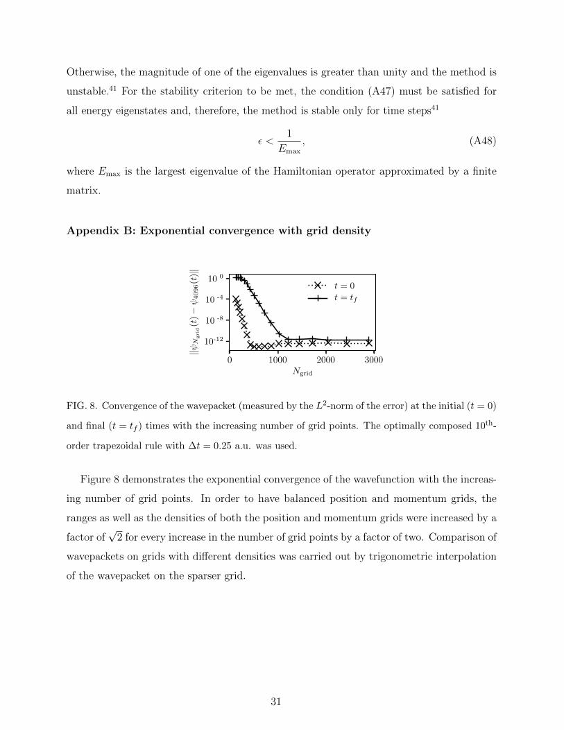
Appendix B: Exponential convergence with grid density

0 1000 2000 3000Ngrid

10 0

10 -4

10 -8

10-12

‖ψN

grid

(t)−ψ

4096(t

)‖

t = 0

t = tf

FIG. 8. Convergence of the wavepacket (measured by the L2-norm of the error) at the initial (t = 0)

and final (t = tf ) times with the increasing number of grid points. The optimally composed 10th-

order trapezoidal rule with ∆t = 0.25 a.u. was used.

Figure 8 demonstrates the exponential convergence of the wavefunction with the increas-

ing number of grid points. In order to have balanced position and momentum grids, the

ranges as well as the densities of both the position and momentum grids were increased by a

factor of√

2 for every increase in the number of grid points by a factor of two. Comparison of

wavepackets on grids with different densities was carried out by trigonometric interpolation

of the wavepacket on the sparser grid.

31

REFERENCES

1M. Born and R. Oppenheimer, Ann. Phys. 389, 457 (1927).

2E. J. Heller, The semiclassical way to dynamics and spectroscopy (Princeton University

Press, Princeton, NJ, 2018).

3A. Mokhtari, P. Cong, J. L. Herek, and A. H. Zewail, Nature 348, 225 (1990).

4M. Baer, Beyond Born-Oppenheimer: Electronic Nonadiabatic Coupling Terms and Con-

ical Intersections, 1st ed. (Wiley, 2006).

5W. Domcke and D. R. Yarkony, Annu. Rev. Phys. Chem. 63, 325 (2012).

6H. Nakamura, Nonadiabatic Transition: Concepts, Basic Theories and Applications, 2nd

ed. (World Scientific Publishing Company, 2012).

7K. Takatsuka, T. Yonehara, K. Hanasaki, and Y. Arasaki, Chemical Theory Beyond the

Born-Oppenheimer Paradigm: Nonadiabatic Electronic and Nuclear Dynamics in Chemical

Reactions (World Scientific, Singapore, 2015).

8M. P. Bircher, E. Liberatore, N. J. Browning, S. Brickel, C. Hofmann, A. Patoz, O. T.

Unke, T. Zimmermann, M. Chergui, P. Hamm, U. Keller, M. Meuwly, H. J. Woerner,

J. Vanıcek, and U. Rothlisberger, Struct. Dyn. 4, 061510 (2017).

9S. Shin and H. Metiu, J. Chem. Phys. 102, 9285 (1995).

10J. Albert, D. Kaiser, and V. Engel, J. Chem. Phys. 144, 171103 (2016).

11A. Abedi, N. T. Maitra, and E. K. Gross, Phys. Rev. Lett. 105, 123002 (2010).

12L. S. Cederbaum, J. Chem. Phys. 128, 124101 (2008).

13T. Zimmermann and J. Vanıcek, J. Chem. Phys. 132, 241101 (2010).

14T. Zimmermann and J. Vanıcek, J. Chem. Phys. 136, 094106 (2012).

15M. Ben-Nun, J. Quenneville, and T. J. Martınez, J. Phys. Chem. A 104, 5161 (2000).

16B. F. E. Curchod and T. J. Martınez, Chem. Rev. 118, 3305 (2018).

17D. V. Shalashilin and M. S. Child, J. Chem. Phys. 115, 5367 (2001).

18D. V. Makhov, C. Symonds, S. Fernandez-Alberti, and D. V. Shalashilin, Chem. Phys.

493, 200 (2017).

19G. A. Worth, M. A. Robb, and I. Burghardt, Faraday Discuss. 127, 307 (2004).

20G. Richings, I. Polyak, K. Spinlove, G. Worth, I. Burghardt, and B. Lasorne, Int. Rev.

Phys. Chem. 34, 269 (2015).

21H.-D. Meyer, U. Manthe, and L. S. Cederbaum, Chem. Phys. Lett. 165, 73 (1990).

32

22G. A. Worth, H.-D. Meyer, H. Koppel, L. S. Cederbaum, and I. Burghardt, Int. Rev.

Phys. Chem. 27, 569 (2008).

23H. Wang and M. Thoss, J. Chem. Phys. 119, 1289 (2003).

24G. Avila and T. Carrington Jr, J. Chem. Phys. 147, 144102 (2017).

25C. Lubich, From Quantum to Classical Molecular Dynamics: Reduced Models and Numer-

ical Analysis, 12th ed. (European Mathematical Society, 2008).

26R. Kosloff, J. Phys. Chem. 92, 2087 (1988).

27E. Hairer, C. Lubich, and G. Wanner, Geometric Numerical Integration: Structure-

Preserving Algorithms for Ordinary Differential Equations (Springer Berlin Heidelberg

New York, 2006).

28L. Verlet, Phys. Rev. 159, 98 (1967).

29D. Frenkel and B. Smit, Understanding molecular simulation, 2nd ed. (Academic Press,

2002).

30E. A. McCullough, Jr. and R. E. Wyatt, J. Chem. Phys. 54, 3578 (1971).

31M. D. Feit, J. A. Fleck, Jr., and A. Steiger, J. Comp. Phys. 47, 412 (1982).

32D. J. Tannor, Introduction to Quantum Mechanics: A Time-Dependent Perspective (Uni-

versity Science Books, Sausalito, 2007).

33H. Yoshida, Phys. Lett. A 150, 262 (1990).

34R. I. McLachlan, SIAM J. Sci. Comput. 16, 151 (1995).

35M. Suzuki, Phys. Lett. A 146, 319 (1990).

36M. Wehrle, M. Sulc, and J. Vanıcek, Chimia 65, 334 (2011).

37J. Roulet, S. Choi, and J. Vanıcek, Unpublished.

38B. Leimkuhler and S. Reich, Simulating Hamiltonian Dynamics (Cambridge University

Press, 2004).

39A. Askar and A. S. Cakmak, J. Chem. Phys. 68, 2794 (1978).

40D. Kosloff and R. Kosloff, J. Comp. Phys. 52, 35 (1983).

41C. Leforestier, R. H. Bisseling, C. Cerjan, M. D. Feit, R. Friesner, A. Guldberg, A. Ham-

merich, G. Jolicard, W. Karrlein, H.-D. Meyer, N. Lipkin, O. Roncero, and R. Kosloff,

J. Comp. Phys. 94, 59 (1991).

42C. Lubich, “Quantum simulation of complex many-body systems: From theory to algo-

rithms, lecture notes,” (John von Neumann Institute for Computing, Julich, 2002) Chap.

Integrators for quantum dynamics: A numerical analyst’s brief review, pp. 459–466.

33

43H. Tal-Ezer and R. Kosloff, J. Chem. Phys. 81, 3967 (1984).

44C. Lanczos, J. Res. Nat. Bur. Stand. 45, 255 (1950).

45T. J. Park and J. C. Light, J. Chem. Phys. 85, 5870 (1986).

46J. Crank and P. Nicolson, Math. Proc. Camb. Phil. Soc. 43, 50 (1947).

47V. Engel and H. Metiu, J. Chem. Phys. 90, 6116 (1989).

48G. Stock, C. Woywod, W. Domcke, T. Swinney, and B. S. Hudson, J. Chem. Phys. 103,

6851 (1995).

49J. Auslander, N. Bhatia, and P. Seibert, Bol. Soc. Mat. Mex. 9, 55 (1964).

50N. P. Bhatia and G. P. Szego, Dynamical systems: stability theory and applications, Vol. 35

(Springer, 2006).

51G. H. Golub and C. F. Van Loan, Matrix Computations, 3rd ed. (The Johns Hopkins

University Press, 1996).

52W. H. Press, S. A. Teukolsky, W. T. Vetterling, and B. P. Flannery, Numerical Recipes,

The art of scientific computing, 3rd ed. (Cambridge University Press, 2007).

53Y. Saad and M. H. Schultz, SIAM J. Sci. Stat. Comp. 7, 856 (1986).

54Y. Saad, Iterative Methods for Sparse Linear Systems, 2nd ed. (SIAM, 2003).

55W. E. Arnoldi, Quart. Appl. Math 9, 17 (1951).

56Y. Saad, Linear Algebra Appl. 34, 269 (1980).

57M. Creutz and A. Gocksch, Phys. Rev. Lett. 63, 9 (1989).

58E. Forest and R. D. Ruth, Physica D 43, 105 (1990).

59W. Kahan and R.-C. Li, Math. Comput. 66, 1089 (1997).

60M. Sofroniou and G. Spaletta, Optim. Method Softw. 20, 597 (2005).

61R. Kosloff and D. Kosloff, J. Chem. Phys. 79, 1823 (1983).

62R. G. Sadygov and D. R. Yarkony, J. Chem. Phys. 109, 20 (1998).

63M. Baer and R. Englman, Mol. Phys. 75, 293 (1992).

64W. D. Hobey and A. D. McLachlan, J. Chem. Phys. 33, 1695 (1960).

65H. Tal-Ezer, J. Sci. Comput. 4, 25 (1989).

66P. R. Halmos, Finite dimensional vector spaces (Princeton University Press, 1942).

67P. R. Halmos, Introduction to Hilbert space and the theory of spectral multiplicity (Chelsea,

1951).

68G. W. Stewart, Matrix algorithms, Vol. 1 (SIAM, 1998).

34