Laughter Detection in Noisy SettingsMary Felkin, Jeremy Terrien and Kristinn R. Thorisson

Technical Report number CS09002

1 IntroductionThe importance of laughter in human relationships can hardly be contested; its importance in communication has beenpointed out by a number of authors (cf. [11] [15] [18]). Like some of those working on analysis of audio data beforeus [26] [37], a future goal of our work is to be able to classify many types of non-speech vocal sounds. The approachwe use in this work relies upon machine learning techiques, as it could take centuries to hand-code algorithms fordetecting laughter and other sounds, which have high variability both between cultures and between individuals. Herewe describe our application of C4.5 to find the onset and offset of laughter using single-speaker audio recordings. Priorefforts using machine learning for this purpose have focused on several techniques, but no one, to our knowledge, hasused C4.5.

Unlike much of the prior work on laughter detection (although see [16] [36]) our ultimate aim is not simply thedetection of laughter but the use of this information – by a robot or virtual humanoid – to produce the appropriateconversational responses in realtime dialogue with people. Such a system could also be used to improve speechrecognition by eliminating periods of non-speech sound. As false positives constitute a significant portion of speechrecognition errors, a high-quality solution in this respect could be expected to improve speech recognition considerably.

Many prior papers on automatic laughter detection leave out details on the average duration of the laughter andonly mention the length of the full recordings containing (one or more bursts of) laughter – these presumably beingthe recordings that got them the best results. In our corpus laughter duration of 2.5 seconds produced the highestaccuracy. Because of our interest in realtime detection we analyze our recordings not only at this length, to produce abest-possible result, but also at sub-optimal sample duration, from 150 msecs up to the full length of our samples of 3seconds. We discuss the results of this analysis in light of our realtime goals.

Our audio is collected with a close microphone and the audio is relatively clean; however the duration of laughtervaries from 0.5 to 5 seconds. Additionally, the negative examples include not only speech but also other non-laughtergeneral vocal sounds. These were generated by instructing subjects to “make sounds that are not laughter but youthink might be confused with laughter”. We have used the context of a television interview scenario as a way to focusthe work on a practical scenario. In such a scenario each person would be carrying a clip-on microphone but withfar-from-perfect noise control, and thus all our data has been recorded with a moderate amount of background noise.

We use an auto-regression algorithm to produce a set of descriptors for the sound samples and segments thereof.The output of this signal processing stage (what would be called “pre-processing” in the machine learning community)shows exremely high correlation for each individual descriptor between laughter and non-laughter samples, meaningthat discerning their difference using our descriptors is difficult and error prone. This motivates in part the use ofmachine learning. It may not be immediately obvious that C4.5 should be applied to the task of laughter detection.However, we report better result than the best that we are aware of yet in the literature. This will serve as a pointof comparison when we go to solutions that work faster, for realtime purposes. Once trained on the data the C4.5algorithm is extremely fast to execute, since it is represented as a set of If-Then rules. This caters nicely to anyrealtime application.

The paper is organized as follows: After a review of related work we describe the signal processing algorithmsemployed and show how correlated their output is. Then we describe the results from training C4.5 on the corpus andpresent the results of applying it to new data.

2 Related WorkA number of papers have been published on the application of learning for detecting the difference between speech andlaughter in audio recordings [15] [35] [9] [34] [11]. The work differs considerably on several dimensions includingthe cleanliness of data, single-person versus multiple-person soundtracks, as well as the learning methods used. Rea-sonable results of automatic recognition have been reported using support vector machines [35], [9], Hidden MarkovModels [15] [18], artificial neural nets [11] [35] and Gaussian Mixture Models [35], [34]. Some of the studies ([5],[11], [34], [35], [9], [14], [31], [24] and [15]) relie on very expensive databases such as the ICSI meeting corpus [1]and [23]. Use of a common corpus might make one think it possible to easily compare results between studies. Thestudies, however, pre-process data in many ways, from manual isolation of laughter versus non-laughter segments, tocompletely free-form multi-party recordings. They are therefore not easily comparable. [8] describes a classification

1

experiment during which fourteen professional actors recorded themselves reading a few sentences and expressed, ineach recording, an emotion chosen among {neutral, hapiness, sadness, anger}. The authors do not give their results.[19] classifies laughter versus non-laughter from among 96 audio-visual sequences and uses visual data to improveaccuracy. [20] also describes audio-visual laughter detection, based on temporal features and using perceptual linearprediction coefficients. Among the highest reported recognition rate for audio alone was that of [11], which reportedonly 10% misses and 10% false positives, with a 750msecs sample length, using a neural network on clean data.Finally, [28] gives a review of multimodal video indexing.

Among the methods used for pre-processing are mel-frequency cepstral coefficients (MFCCs) [11] [35] (see alsothe seminal work introducing their use for audio processing: [32]). Perceptual Linear Prediction features are also apossibility: [34] for a an example of related use and [6] for a more general discussion.

Among other laugh-related studies are [13] which describes the phonetics of laughter. It is not a classificationexperiment. [2] studies how people react to different types of laughter. [30] describes relationships between breathingpatterns and laughter. [36] uses multimodal laughter detection to make a “mirror” which distorts the face. The morethe person laughs at the distortion, the more distorted the picture gets. [18] differentiate between types of laugh: forJapanese speakers, some words are considered to be laugh. Related to it is [27] about clustering audio according to thesemantics of audio effects. [29] tackles the inverse problem: laughter synthesis. The wide spectrum of laugh-relatedstudies, of which these are but a small sample, encompass, without being restricted to, pychology, cognitive scienceand philosophy as well as acoustics, giving to our topic an important place in any field related to intelligence and tocommunication.

3 Data CollectionSound samples were collected through a user-friendly interface; subjects were volunteers from Reykjavik University’sstaff and student pool. Recordings were done in a relatively noisy environment (people talking and moving in thebackground, and often people hanging around while the recording was achieved) using a microphone without noisecancellation mechanisms.

The volunteers were asked to:

• Record 5 samples of him/herself laughing

• Record 5 samples of him/herself speaking spontaneously

• Record 5 samples of him/herself reading aloud

• Record 5 samples of him/herself making other sounds

The other noises recorded included humming, coughing, singing, animal sound imitations, etc. One volunteerthought that rythmic hand clapping and drumming could also be confused with laughter so he was allowed to producesuch non-vocal sounds.

The instructions to each participant were to “Please laugh into the microphone. Every sample should last at leastthree seconds.” For the non-laughter sounds we instructed them that these could “include anything you want. Wewould appreciate it if you would try to give us samples which you think may be confused with laughter by a machinebut not by a human. For example, if you think the most discriminant criteria would be short and rythmic bursts ofsound, you could cough. If you think phonemes are important, you could say “ha ha ha” in a very sad tone of voice,etc.”.

The University cosmopolitan environment allowed us to record speech and reading in several different languages,the volunteers were encouraged to record themselves speaking and reading in their native languages.

4 Signal Processing Using CUMSUMWe assume that each phoneme can be defined as a stationary segment in the recorded sound samples. Several algo-rithms have been developed to extract the stationary segments composing a signal of interest. In a first approach, we

2

chose a segmentation algorithm based on auto-regressive (AR) modeling, the CUMSUM (CUMulated SUMs) algo-rithm [25]. Other methods have been tried, for example [33], and [17] gives a method for segmenting videos. Thepupose is classification according to the genre of the movie (science fiction, western, drama, etc.).

In a change detection context the problem consists of identifying the moment when the current hypothesis startsgiving an inadequate interpretation of the signal, so another hypothesis (already existing or created on the fly) becomethe relevant one. An optimal method consists in recursive calculation, at every time step, of the logarithm of thelikelihood ratio Λ(xt). This is done by the CUMSUM algorithm [3].

The constants in the equations were tuned for the particular corpus we used; these have not yet been compared toresults on other samples so we cannot say, at the moment, how particular they are to our recordings. However, we donot expect these to be significantly different for any general recordings done by close-mic, single user data sets as weused standard PC equipment and an off-the-shelf microphone to collect the data.

4.1 The CUMSUM algorithmH0 and H1 are two hypothesisH0 : xt, t ∈]0, k] where xt follows a probability density f0

H1 : xt, t ∈]k, n] where xt follows a probability density f1

The likelihood ratio Λ(xt) is defined as the ratio of the probability densities of x under both hypothesis (equation1).

Λ(xt) =f1(xt)

f0(xt)(1)

The instant k of change from one hypothesis to the other can then be calculated according to [3], [7] and [4](equations 2 and 3).

K = inf{n ≥ 1 : max

t∑

j=1

logΛ(xj) ≥ λ0}; 1 ≤ t ≤ n (2)

K = inf{n ≥ 1 : Sn − min St ≥ λ0}; 1 ≤ t ≤ n (3)

Where St is the cumulated sum at time t, defined according to equation 4.

St =n∑

t=1

logΛ(xt); S0 = 0 (4)

In the general case, with several hypotheses, the detection of the instant of change k is achieved through thecalculation of several cumulated sums between the current hypothesis Hc and each of the N hypotheses alreadyidentified.

∀ Hi hypothesis

S(t, i) =t∑

j=1

logΛ(xj) (5)

Λi(xn) =fc(xn)

fi(xn)(6)

Where :

fc is the probability density function of x under the current hypothesis Hc

fi is the probability density function of x under Hi hypothesis for i ∈ {1, ..., N}

3

We define a detection functionD(t, i) = max S(n, i)−S(t, i) for i ∈ {1, ..., N}. This function is then comparedto a threshold λ in order to determine the instant of change between both hypotheses.

In several instances the distribution parameters of random variable x, under the different hypothesis, are unknown.As a workaround, the likelihood ratios used by CUMSUM are set according to either signal parameters obtained fromAR modeling or the decomposition of the signal into wavelets by wavelet transform [10].

4.1.1 Breakpoint detection after AR modeling

When the different samples xi of a signal are correlated, these samples can be expressed by an AR model (equation 7).

xi +q∑

k=1

akxi−k = εi; εi ∈ N(0,σ) (7)

Where :

εi is the prediction error

a1, ..., ak are the parameters of the AR model

q is the order of the model

If x follows a Gaussian distribution the prediction errors εi also follow a Gaussian distribution and are not corre-lated. In this case the logarithm of the likelihood ratio of the prediction errors Λ(εi) can be expressed under H0 andH1 hypothesis as in [10] (equation 8).

log(Λ(εi)) =1

2log

σ20

σ21

+1

2((εi,0)2

σ20

−(εi,1)2

σ21

) (8)

Where :

σ2j is the variance of the prediction error under the jth hypothesis

εi,j is the prediction error under the jth hypothesis

When several hypotheses exist, the likelihood ratio between the current hypothesisHc and every already identifiedhypothesis is calculated. The cumulated sum S(n, i) at time n between the current hypothesis and the ith hypothesisis calculated according to equation 9.

S(n, i) = S(n − 1, i) +1

2log

σ2c

σ2i

+1

2((εt,c)2

σ2c

−(εt,i)2

σ2i

) (9)

The detection function D(t, i) is defined:D(t, i) = max S(t, i)S(n, i)for 1 ≤ t ≤ nThe instant of change is detected whenever one of the M detection functions reaches a λ0 threshold. Although

temporal issues are subject to future work, it should be noted that there exists a detection time lag τ introduced bydetection functionD(t, i).

5 Attribute Construction for ChunksTo separate audio segments from silence segments we applied an energy threshold on each detected stationary segment.We chose to keep all segments that represent 80% of the energy of the original signal. All non-selected segments whereconsidered silence and discarded from further analysis. All contiguous phonemes where then mixed to form a burst.

For each burst Wi we first computed their fundamental frequency, defined as the frequency of maximal energy inthe burst’s Fourier power spectrum. The power spectrum of the burst i (Pxxi(f)) was estimated by averaged modifiedperiodogram. We used a Hanning window of one second duration with an overlap of 75%. The fundamental frequencyFi and the associated relative energy Ereli are then obtained according to equations 10 and 11.

4

Fi = argmaxf Pxxi (f) (10)

Ereli =max (Pxxi(f))∑Fs

2f=0

Pxxi (f)(11)

where Fs is the sampling frequency.We also considered the absolute energy Ei, the length Li and the time instant Ti of each burst. Their use can be

seen in the decision tree.

5.1 Burst SeriesA burst series is defined as a succession of n sound burst bursts. The number of bursts is not constant from one seriesto another. Our approach to pre-processing for audio stream segmentation was based on the following hypotheses:

1. F. Maximum energy frequency: The fundamental frequency of each audio burst is constant or slowly varying.No supposition has been made concerning the value of this parameter since it could vary according to the genderof the speaker (we performed no normalisation to remove these gender-related differences in vocal tract length).It could also vary according to the particular phoneme pronounced during the laugh, i.e.“hi hi hi” or “ho ho ho”,or, as some native Greenanders’ laugh, “t t t”.

2. Erel. Relative energy of the maximum: The relative energy of the fundamental frequency of each burst isconstant or slowly varying. This parameter should be high due to the low complexity of the phoneme.

3. E. Total energy of the burst: The energy of each burst is slowly decreasing. The laugh is supposed to beinvoluntary and thus no control of the respiration to maintain the voice level appears. This is, as we will see,a useful criterion because when a human speaks a sentence, he or she is supposed to control the volume ofeach burst in order to maintain good intelligibility and this control for the most part only breaks down whenexpressing strong emotions.

4. L. Instant of the middle of the burst: The length of each burst is low and constant due to the repetition of thesame simple phoneme or group of such.

5. T. Length of the burst: The difference between consecutive burst occurence instants is constant or slowly vary-ing. A laugh is considered as an emission of simple phonemes at a given frequency. No supposition concerningthe frequency was done since it could vary strongly from one speaker to the other. At the opposite, a nonlaughing utterance is considered as a “random” phoneme emission.

6. Te. Total energy of the spectre’s summit: Same as 2. but not normalised according to the total energy of theburst.

To differentiate records corresponding to a laugh or a non-laugh utterance, we characterised each burst series bythe regularity of each parameter. This approach allowed us to be independent of the number of bursts in the recordedburst series. For the parameters Fi,Ereli,Ei and Li, we evaluated the median of the absolute instantaneous differenceof the parameters. For the parameter Ti, we evaluated the standard deviation of the instantaneous emission period, i.e.Ti+1 − Ti.

5.2 Burst Series Characterisation: Details of Attribute ConstructionThe input is an array of floats. The sound samples were recorded in mono (using one audio channel of the uncom-pressed .wav format).

We segment the array into “bursts”. Fig.1 shows 3 bursts. The horizontal axis is time, the vertical axis is the sound.We take the first 512 points. We dot-multiply them by a vector of 512 points distributed along a gaussian-shaped

curve according to Hanning’s function (equation 12 and fig.3). Fig.2 illustrates this process, showing a burst (left)multiplied by points distributed according to Hannings’ function (center) and the resulting normalisation (right).

5

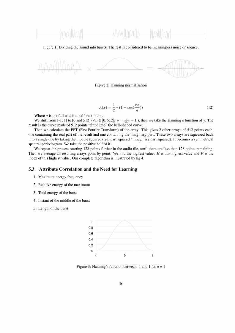
Figure 1: Dividing the sound into bursts. The rest is considered to be meaningless noise or silence.

Figure 2: Hanning normalisation

A(x) =1

2∗ (1 + cos(

πx

a)) (12)

Where a is the full width at half maximum.We shift from [-1, 1] to [0 and 512] (∀x ∈ [0, 512]; y = x

256− 1 ), then we take the Hanning’s function of y. The

result is the curve made of 512 points “fitted into” the bell-shaped curve.Then we calculate the FFT (Fast Fourier Transform) of the array. This gives 2 other arrays of 512 points each,

one containing the real part of the result and one containing the imaginary part. These two arrays are squeezed backinto a single one by taking the module squared (real part squared * imaginary part squared). It becomes a symmetricalspectral periodogram. We take the positive half of it.

We repeat the process starting 128 points further in the audio file, until there are less than 128 points remaining.Then we average all resulting arrays point by point. We find the highest value. E is this highest value and F is theindex of this highest value. Our complete algorithm is illustrated by fig.4.

5.3 Attribute Correlation and the Need for Learning1. Maximum energy frequency

2. Relative energy of the maximum

3. Total energy of the burst

4. Instant of the middle of the burst

5. Length of the burst

Figure 3: Hanning’s function between -1 and 1 for a = 1

6

Figure 4: The complete algorithm

7

Figure 5: Attribute 1

6. Total energy of the spectre’s summit

No single descriptor on it’s own is sufficient to differentiate laughter vs. non laughter samples. Figures 5, 6, 7, 8and 9 represent the probability densities (Y-axis) of the attribute values (X-axis). For comparison purposes a summedhistogram is given in fig.10. This indicates that there is no trivial method to differenciate laughter from non-laughtersamples, using our descriptors, and supervised classification techniques are required. We solved this problem with thedecision tree inducer C4.51 [21] [22].

5.4 Sensitivity to preprocessing parametersWe used Mayavi to map the results of different parameter values in 3D boxes. Mayavi shows the location of allaccuracy results within a specified range in parameter space, as illustrated by fig. 12. In fig. 13 the low accuraciesare on the left and the better ones on the right. The top to bottom rows represent the fourth dimension created bymodifying the values of parameter ”Taille Fen” which represents the length of the Hanning window (the best one, onesecond with 75% overlap, is the fourth row of boxes).

It can be seen from figs. 12 and 13 that this program requires careful tuning in order to obtain good results.

5.5 Shortening Sample Duration Weeds Out Troublesome ExamplesIn the following experiments we tried reducing the length of the samples. In figs. 11 to 20, the X axis alwaysrepresents the percentage of the sound file which has been used. These percentages go from 5% (0.15 seconds) to100% (3 seconds).

But the preprocessing we use skips samples when they do not contain enough information. The comparison-based descriptors cannot compare bursts when they have a single or no “burst”. The files corresponding to the shortersamples are full of zeroes, for example the average distance between two consecutive bursts is set to zero when there isonly one burst. When nothing meaningful is found no output is produced. Even when the samples do contain enough

1We tried a few classification algorithms which met the following criteria: generating explicit models, being readily available and being fast.C4.5 turned out to be the best predictor of our class attribute among them.

8

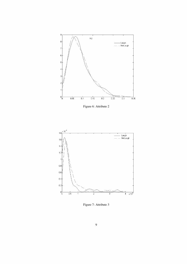
Figure 6: Attribute 2

Figure 7: Attribute 3

9

Figure 8: Attribute 4

Figure 9: Attribute 5

10

Figure 10: Attribute Values

Figure 11: Number of samples

11

Figure 12: Parameter space

12

Figure 13: Location of accuracy results

13

information to provide a numerical result, this result is sometimes not significant (for example, Matlab considers thatthe standard deviation of the two numbers 1 and 2 is 0.7, for a reason we do not know). Fig.11 shows the number oflaughter and on-laughter examples we have for the different durations.

Analysis starts from beginning of the sound file, not from the first burst occurrence. A better result could verylikely be achieved for the shorter samples if analysis started with the first burst in each sound file.

As it is, the results corresponding to the shorter samples should be treated with suspicion, as the pre-processinghas only kept the “best behaved” samples. Only in the range [75%, 100%] do we have all the examples. In [35%, 70%]not more than 6 samples have been removed. At 5% only 67 out of 235 samples remain. For various mathematicalreasons, when the calculations cannot be performed the example is ignored, so the smaller databases comprise onlythe calculable examples. Replacing all uncalculable values by zeros did not appear to be a good solution because itwould overwelm meaningfull zeros, and setting an arbirary value (or an extra attribute) to mean ”uncalculable” wasconsidered and rejected because we did not want our attributes to be given arbitrary values.

6 Supervised Classification: Primary resultsCross-validation is the practice of partitioning a set of data into subsets to perform the analysis on a single subsetwhile the others are used for training the classification algorithm. This operation is repeated as many times as thereare partitions. In the following, except where otherwise mentioned, we use 10 − folds cross validation, which meanswe train on 90% of the samples and test on the remaining 10%. We do this 10 times and average the results. In thisway, our accuracy is a good (if slightly pessimistic2 [12]) estimator of what our accuracy would be upon unknownexamples.

6.1 Laughter vs. non-laughterFig.14 shows that 3 seconds is too long: In many samples, people had not been able to laugh during 3 seconds, so thetail of the sound file is noise. It also happens with spontaneous speech and other noises. Our best results were:

• Sample length = 75%, accuracy = 88.6%

• Sample length = 80%, accuracy = 88.1%

• Sample length = 85%, accuracy = 89.5%

Figure 14: laughter vs. non-laughter, realtime results.

14

Figure 15: Training on full length samples and testing on shorter lenghs samples

6.2 Shortening the sample length: ResultsIn fig.15, the Y axis is the result of using the 100% length dataset as a training set and the datasets corresponding to theshorter lengths as test set. So this experiment does not use cross validation. The 97.4% accuracy achieved at the 100%length is the result of using the same set for training and testing, and as such should not be considered as a dataminingresult. The previous fig shows that “real” accuracy for this is 86.4%.

These are nevertheless interesting for comparison purposes between shorter and longer sample datasets.Smooth upgoing line from 35% to 100%. Gets wobbly in the lower region from 5% to 30% This wobbliness could

indicate that the results are less and less precise, in the sense that with another set of recording samples we could getresults which are more different one from the other in the lower region for the same sample length.

It is interesting to note how a decision tree (the one reproduced below), which can restitute its own dataset with97.4% accuracy and has 86.6% 10-folds cross validation accuracy, completely fails on shorter samples. When thelengths are between 5% and 20% (included), the accuracy is actually lower than 50% (which means that a classifiergiving random predictions would do better on average).

The decision tree on the full length samples is shown in the appendix.

7 Supervised Classification: Secondary Results7.1 Multi-class values experimentsIn two further experiments, we tested the ability of our system to differentiate between the three non-laughter types.In the first experiment, we ran our classifier on a database where the samples were labeled according to 3 possiblevalues: Laughter, Reading and Speech. The ”Other sounds” samples were excluded. In the second one all sampleswere included and so the class had four possible values, laughter, Reading, Speech and Others.

7.1.1 laughter, reading or speech

In fig.16, the Y axis is the result of using 10-folds cross-validation on the ternary datasets where the class can have thevalues of laughter, Reading or Speech. The “Other sounds” samples were removed from the databases.

For comparison purposes, results were transformed into their binary equivalent.

7.1.2 laughter, Reading, Speech or Others Sounds

In fig.17, the Y axis is the result of using 10-folds cross-validation on the quaternary datasets where the class can havethe values of laughter, Reading, Speech or Other sounds.

For comparison purposes, results were transformed into their binary equivalent.2because we only build the classification models upon which we calculate the acuracy on 90% of the examples instead of 100%. When the

number of examples is limited, increasing the number of training examples tends to increase the accuracy

15

Figure 16: laughter, Reading or Speech

Figure 17: laughter, Reading, Speech or Others Sounds

7.1.3 Comparing results across experiments where the number of possible class values differs

The results were transformed into their binary equivalent according to equation 13.

acc2 = acclog(2)log(N)

N (13)

Where N is the number of possible class values, accN the accuracy obtained on the N class values problem andacc2 the equivalent binary accuracy.

In fig.18, dark blue is the original experiment, light blue is the ternary experiment and light green is the quaternaryexperiment. It shows our system, designed specifically for laughter detection, performs poorly on other tasks.

7.2 Reading or SpeechTo explain the poor results illustrated by fig.18, we show in fig.19 that our system is not meant to differentiate be-tween Reading and Speech. This binary experiment, during which the samples correspondig to laughter and thesecorresponding to the other sounds were removed from the databases, shows that any experiment which implies differ-entiating between Reading and Speech is bound to have poor results. (In order not to miss how poor these results are,it should be noted that the Y axis only goes up to 70 in fig.19).

7.3 laughter or Spoken soundsFinally, we tried without the “Other sounds” examples. These results appear in red in the fig.20 while the originalresults are in dark blue. We were wondering whether these other sounds could be detrimental to the results, by beingeasily confused with laughter. It turned out they were only slightly so.

16

Figure 18: Comparisons: dark blue is binary, light blue is ternary and green is quaternary experiment

Figure 19: Reading or Speech

Figure 20: laughter or Spoken sounds

7.4 Combining sound files of different lengthsThe matrices illustrated by fig.21 and fig.22 are the same, shown under different angles.

Combining sound files of different lengths improves accuracy for the shorter samples. Matrices 1 show crossvalidation performed on set containing examples of length 0.15 seconds to 3 seconds. On the diagonal only examplesof one length were used, so there was no hidden repetition of examples or of part of examples.

As we go away from the diagonal the databases contain examples of length 0.15 and 0.3; then 0.15, 0.3 and 0.45,etc, until on the corner we have all examples, from 0.15 to 0.3 seconds.

This result is biased because the samples of length, say, 0.15 and 0.3 seconds, are not completely distinct. They arecalculated from the same sound samples, each example of length 0.15 is the half of one example of length 0.3. Proper

17

Figure 21: Matrix 1

Figure 22: Matrix 1 (different angle)

Figure 23: Matrix 2

cross validation would require separating the examples into 10 subsets right at the start of the experiment (beforepre-processing the sound files) otherwise, as some examples get dropped in the preprocessing, they cannot be tracked.

Matrix 2 in fig.23 was generated without cross validation: on it the advantage gained by repeating examples (whichpulled the diagonal on matrix 1 downwards) is gone. So around 1 or 2% can be gained by combining examples of

18

different lengths, on the longer segments. The shorter samples are much more unpredictable. Still, we reach accuracies> 80% more quickly this way, (which will be important when the speed of the classfication will matter).

This is also an advance with respect to the state of the art, as far as we know no-one had investigated this aspectbefore.

8 Summary of best resultsLength Accuracy with other sounds Accuracy without other sounds75% 88.6% 86.4%80% 88.1% 88.8%85% 89.5% 89.6%90% 86.1% 85.2%95% 84.4% 87.6%100% 86.4% 85.2%

9 Towards Laughter Detection in Realtime SystemsSo far we have been focused on classification accuracy of laughter. However, using such information in dialoguecalls for processing speed with a particular recognition reliability. It would do the artificial host of television-showno good if his recogition of laughter happened 5 seconds after the laughter was detected; unnatural responses wouldbe certain to unsue. Ideally detection of laughter in a realtime system has minimum latency and maximum accuracy;given that these can of course never be 0 and 100%, respectively, one has to construct the system in such a way as tohave a reasonable speed/accuracy tradeoff. Ideally, that tradeoff is controlled by the system itself. Two ways to do thatwould be to either allow that to be set prior to the processing of the live stream or, a better alternative, to implement ananytime algorithm that, for every minimal time sampling period outputs a ¡guess, certainty¿ value par, and then keepsupdating the guess and its certainty as more processing is done on the signal.

To expand the system built so far to such a system we have made the sound processing functions free-standingexecutables which talk to each other via streams. The sound files are now streamed through such a pipeline, simulatinglive audio streaming (the latter of which can also be done in the new system). In our current setup, sound capturedfrom the sound card is sent to the RAM in bursts of 1kB (about 0.1 second) in a succession unsigned floats (16 bitslong). The results of this work will be detailed in a later report.

19

10 ConclusionsLaughter is important. Among all possible non-verbal sounds, laughing and crying are these which carry the strongestemotional-state related information. Their utterance predates language skills acquisition by newborn babies. Laughteris typically human, with the possible inclusion of some other primates. Crying and related sounds emitted by youngsfor the purpose of attracting the attention and care of adults belonging to the same specie3 is common accross mostmammal species. In the framework of inter-adult communication, laughter could be the non-verbal sound which is themost meaningfull while still being relatively common.

C4.5 is well known as being a robust multi-purpose algorithm. What has been designed specifically for the purposeof recognising laughter are our preprocessing formulas and we have shown that our preprocessing is appropriate forlaughter detection, but useless for other tasks such as distinguishing between reading aloud and spontaneous speech.

We have shown that we do better than the state of the art on audio data, and we are now working on optimising ouralgorithm for real-time uses.

3Cats are an example of specie which has evolved phonetic utterances destined to attract the attention of members of another specie, i.e. humans.

20

References[1] Jane Edwards Dan Ellis David Gelbart NelsonMorgan Barara Peskin Thilo Pfau Elisabeth Shriberg Andreas Stol-

cke Adam Janin, Don Baron and Chuck Wooters. The icsi meeting corpus. Acoustics, Speech, and SignalProcessing, 1:364– I–367, 2003.

[2] Jo-Anne Bachorowski and Micheal J. Owren. Not all laughs are alike: Voiced but not unvoiced really elicitspositive affect. Psychological Science, 12:252–257, 2002.

[3] Nikiforov I Basseville M. Detection of Abrupt Changes, Theory and Application. Prentice-Hall, EnglewoodCliffs, NJ, 1993.

[4] Ghosh BK and Sen PK. Handbook of Sequential Analysis. Marcel Dekker, New York, 1991.

[5] Khiet Truong Ronald Poppe Boris Reuderink, Mannes Poel and Maja Pantic. Decision-level fusion for audio-visual laughter detection. Lecture Notes in Computer Science, 5237, 2008.

[6] H Hermansky. Perceptual linear predictive (plp) analysis of speech. J. Acoust. Soc. Am., 87:1738–1752.

[7] Nikiforov IV. A generalized change detection problem. IEEE Trans. Inform. Theory, 41:171–171.

[8] Eero Vayrynen Juhani Toivanen and Tapio Seppanen. Automatic discrimination of emotion in spoken finnish:Research utilizing the media team speech corpus. Language and Speech, 47:383–412, 2004.

[9] Lyndon S. Kennedy and Daniel P.W. Ellis. Laughter detection in meetings. Proc. NIST Meeting RecognitionWorkshop, 2004.

[10] Duchene J Khalil M. Detection and classification of multiple events in piecewise stationary signals: Comparisonbetween autoregressive and multiscale approaches. Signal Processing, 75:239–251, 1999.

[11] Mary Knox. Automatic laughter detection. Final Project (EECS 294), 2006.

[12] Ron Kohavi. A study of cross-validation and bootstrap for accuracy estimation and model selection. Proceedingsof the Fourteenth International Joint Conference on Artificial Intelligence (IJCAI), 2:11371143, 1995.

[13] Klaus J. Kohler. “speech-smile, “speech-laugh, “laughterand their sequencing in dialogic interaction. JournalPhonetica, 65, 2008.

[14] Kornel Laskowski and Susanne Burger. Analysis of the occurrence of laughter in meetings. Proc. INTER-SPEECH, 2007.

[15] Kornel Laskowski and Tanja Schultz. Detection of laughter in interaction in multichannel close talk microphonerecordings of meetings. Lecture Notes in Computer Science, 5237, 2008.

[16] Laurence Devillers Laurence Vidrascu. Detection of real-life emotions in call centers. Interspeech’2005 - Eu-rospeech, 2005.

[17] Milind R. Naphade and Thomas S. Huang. Stochastic modeling of soundtracks of efficient segmentation andindexing of video. Proc. SPIE 3972, 1999.

[18] Hideki Kashioka Nick Campbell and Ryo Ohara. No laughing matter. Interspeech’2005 - Eurospeech, 2005.

[19] Stavros Petridis and Maja Pantic. Audiovisual discrimination between laughter and speech. Acoustics, Speechand Signal Processing (ICASSP 2008), pages 5117–5120, 2008.

[20] Stavros Petridis and Maja Pantic. Audiovisual laughter detection based on temporal features. InternationalConference on Multimodal Interfaces, pages 37–44, 2008.

[21] J. R. Quinlan. C4.5: Programs for Machine Learning. Morgan Kaufmann Publishers, 1993.

21

[22] J. R. Quinlan. Improved use of continuous attributes in c4.5. Journal of Artificial Intelligence Research, 4:77–90,1996.

[23] Chad Kuyper ad Patrick Menning Rebecca Bates, Elisabeth Willingham. Mapping Meetings Project: GroupInteraction Labeling Guide. Minnesota State University, 2005.

[24] Boris Reuderink. Fusion for audio-visual laughter detection. Technical Report TR-CTIT-07-84, Centre forTelematics and Information Technology, University of Twente, Enschede, 2007.

[25] Mounira Rouainia and Noureddine Doghmane. Change detection and non stationary signals tracking by adaptivefiltering. Proceedings of World Academy of Science, Engineering and Technology, 17, 2006.

[26] Hong-Jiang Zhang Rui Cai and Lian-Hong Cai. Highlight sound effects detection in audio stream. Multimediaand Expo, 2003. ICME ’03, 3:37–40, 2003.

[27] Lie Lu Rui Cai and Lian-Hong Cai. Unsupervised auditory scene categorization via key audio effects andinformation-theoretic co-clustering. Acoustics, Speech, and Signal Processing, 2:1073–1076, 2005.

[28] Cees G.M. Snoek and Marcel Worring. Multimodal video indexing: A review of the state-of-the-art. MultimediaTools and Applications, 2005.

[29] Shiva Sundaram and Shrikanth Narayanan. Automatic accoustic synthesis of human-like laughter. SPEECHPROCESSING AND COMMUNICATION SYSTEMS, 121:527–535, 2007.

[30] Sven Svebak. Respiratory patterns as predictors of laughter. Psychophysiology, 12:62–65, 2008.

[31] Andrey Temko and Climent Nadeu. Classification of meeting-room accoustic events with support vector ma-chines and variable feature set clustering. Acoustics, Speech, and Signal Processing, 5:505–508, 2005.

[32] Jonathan T.Foote. Content-based retrieval of music and audio. Multimedia Storage and Archiving Systems II,Proc. of SPIE., 1997.

[33] Jurgen Trouvain. Segmenting phonetic units in laughter. Proc. 15th. International Congress of Phonetic Sci-ences(ICPhS), 2003.

[34] Khiet P. Truong and David A. van Leeuwen. Automatic detection of laughter. Interspeech’2005 - Eurospeech,2005.

[35] Khiet P. Truong and David A. van Leeuwen. Automatic discrimination between laughter and speech. SpeechCommunication, 49:144–158, 2007.

[36] Marten Den Uyl David A. van Leeuwen Mark A. Neerincx Lodewijk Loos Willen A. Melder, Khiet P. Truongand B. Stock Plum. Affective multimodal mirror: Sensing and eliciting laughter. International MultimediaConference, pages 31–40, 2007.

[37] Christian Zieger. An hmm based system for acoustic event detection. Lecture Notes in Computer Science, 4625,2008.

22

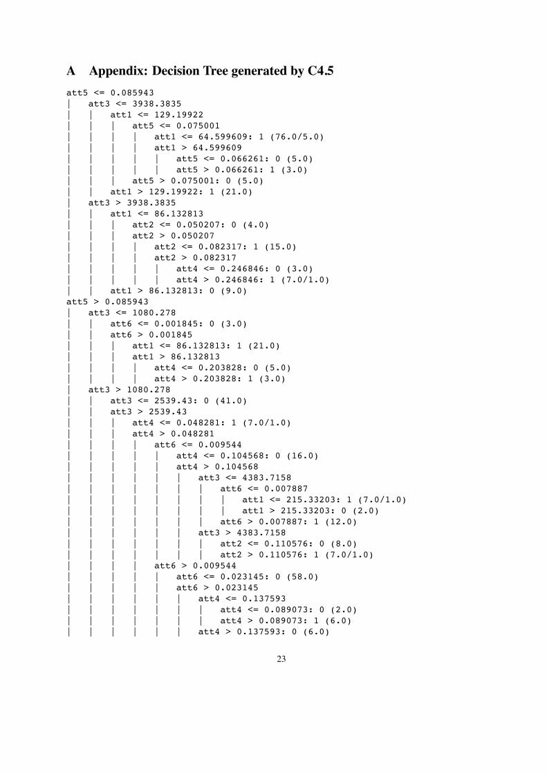
A Appendix: Decision Tree generated by C4.5att5 <= 0.085943| att3 <= 3938.3835| | att1 <= 129.19922| | | att5 <= 0.075001| | | | att1 <= 64.599609: 1 (76.0/5.0)| | | | att1 > 64.599609| | | | | att5 <= 0.066261: 0 (5.0)| | | | | att5 > 0.066261: 1 (3.0)| | | att5 > 0.075001: 0 (5.0)| | att1 > 129.19922: 1 (21.0)| att3 > 3938.3835| | att1 <= 86.132813| | | att2 <= 0.050207: 0 (4.0)| | | att2 > 0.050207| | | | att2 <= 0.082317: 1 (15.0)| | | | att2 > 0.082317| | | | | att4 <= 0.246846: 0 (3.0)| | | | | att4 > 0.246846: 1 (7.0/1.0)| | att1 > 86.132813: 0 (9.0)att5 > 0.085943| att3 <= 1080.278| | att6 <= 0.001845: 0 (3.0)| | att6 > 0.001845| | | att1 <= 86.132813: 1 (21.0)| | | att1 > 86.132813| | | | att4 <= 0.203828: 0 (5.0)| | | | att4 > 0.203828: 1 (3.0)| att3 > 1080.278| | att3 <= 2539.43: 0 (41.0)| | att3 > 2539.43| | | att4 <= 0.048281: 1 (7.0/1.0)| | | att4 > 0.048281| | | | att6 <= 0.009544| | | | | att4 <= 0.104568: 0 (16.0)| | | | | att4 > 0.104568| | | | | | att3 <= 4383.7158| | | | | | | att6 <= 0.007887| | | | | | | | att1 <= 215.33203: 1 (7.0/1.0)| | | | | | | | att1 > 215.33203: 0 (2.0)| | | | | | | att6 > 0.007887: 1 (12.0)| | | | | | att3 > 4383.7158| | | | | | | att2 <= 0.110576: 0 (8.0)| | | | | | | att2 > 0.110576: 1 (7.0/1.0)| | | | att6 > 0.009544| | | | | att6 <= 0.023145: 0 (58.0)| | | | | att6 > 0.023145| | | | | | att4 <= 0.137593| | | | | | | att4 <= 0.089073: 0 (2.0)| | | | | | | att4 > 0.089073: 1 (6.0)| | | | | | att4 > 0.137593: 0 (6.0)

23