LATERAL DISPLACEMENT MAPS OBTAINED FROM

SCANNING PROBE MICROSCOPE IMAGES

by

CHANG SHEN, 1960-

A DISSERTATION

Presented to the Faculty of the Graduate School of the

UNIVERSITY OF MISSOURI-ROLLA

and

UNIVERSITY OF MISSOURI-ST. LOUIS

In Partial Fulfillment of the Requirements for the Degree

DOCTOR OF PHILOSOPHY

in

PHYSICS

1997

Phil B. Fraundorf, Advisor Bernard J. Feldman

Edward B. Hale Oran A. Pringle

Joseph W. Newkirk

© 1997

CHANG SHEN

ALL RIGHTS RESERVED

iii

ABSTRACT

We have investigated a method to study the nanomechanical properties of surfaces by

correlation-based lateral displacement mapping. The method is applicable to all scanning tip

microscopes without additional special hardware. The approach is also relevant to other displacement

mapping tasks, such as stereo image analysis, and can be extended to n-dimensions as well. By studying

lateral differences of two images of essentially the same object, we obtained quantitative information on

either the physical changes of the object or the sample-probe interaction during image acquisition. In

particular, vector lateral displacements were used to study the changes between image pairs and can also

be used to convert a two-dimensional stereo to a three-dimensional topographic map.

We applied this method to the study of surface friction using air-based scanning tunneling

images. By studying the lateral displacement of a pair of scanning tip microscopy images of a hologram

sample, we showed that the lateral displacement map has a doubled spatial frequency in comparison to

the topographic hologram grating structure. A constant normal force model was used to interpret this

result. This explanation works well if the friction force was assumed proportional to the normal force. A

theoretical model was also offered to explain the differences between lateral-force and scanning-force

microscope images.

In order to infer the lateral force from measured lateral displacements, we assumed a continuum

model of tip bending under lateral force. Two approaches, one analytical and one numerical, were

used. The results suggested that tips of some shapes might be very sensitive to lateral forces, enabling

study of scan-dependent transverse forces in high vacuum STM.

iv

ACKNOWLEDGMENTS

The author wishes to express gratitude and appreciation to Professor Philip B.

Fraundorf and Professor Bernard Feldman for their assistance in the preparation of this

manuscript. The author is grateful for their advice and guidance for his research during the six

and half years of happy, yet busy, student life at University of Missouri at St. Louis and

Rolla. The author is also grateful for their consistent encouragement and help.

In addition, special thanks to Dr. Barbara Armbruster of Monsanto, Inc., for her

generous support, including the provision of samples for the study. The author also wishes to

address a deep appreciation to Professor Ta-Pei Cheng. Thanks are also expressed for the

support and encouragement from those professors who helped the author through all the

research and through daily life in St. Louis. Without their help, it would have been impossible

to make any progress in such a drastically different cultural environment.

The author wishes to thank the other members of the dissertation committee for their

help, their valuable input, their suggestions and their participation. They are: Professors

Edward B. Hale, Oran A. Pringle, and Joseph W. Newkirk.

The author thanks the Department of Physics and Astronomy at UM-St. Louis for my

educational and their financial support. Thanks are also extended to UM-St. Louis for

providing the author the opportunity to pursue an advanced degree.

v

The author wishes to thank Mr. Fei Lu, now a new Ph.D., and Mr. Qin Wentao, for their

invaluable discussions, help, and contributions in various aspects of this work. The author

wishes to thank Mr. Wayne Garver for his assistance with laboratory’s equipment. The author

wishes to thank Mike Way for his consistent help with my computer problems. Thanks to Kurt

Pollack, Mike Way, Jeff Tentschert, Mike Meyer, and Kay Brewer for helping me adjust to

American cultural life and the English language. Special thanks goes to Kay Brewer for her

help with English and invaluable discussion. The author wishes also to thank Helen Yi for her

encouragement and support.

vi

TABLE OF CONTENTS

ABSTRACT................................................................................................................ iii

ACKNOWLEDGMENTS ........................................................................................... iv

LIST OF ILLUSTRATIONS..................................................................................... viii

LIST OF TABLES .................................................................................................... xvi

I. THE LITERATURE ON NANOFORCES, DISPLACEMENT MAPPING, AND

SCANNED PROBE MICROSCOPY.................................................................... 1

A. SCANNED PROBE MICROSCOPY ................................................................. 1

B. FORCES AND MECHANICAL PROPERTIES AT THE MICRO AND NANO METER

SCALES..................................................................................................... 7

1. Force Between STM Tip and Sample Surface........................................ 9

2. Force Between AFM Tip and Sample Surface...................................... 10

C. CORRELATION BASED LATERAL DISPLACEMENT MAPPING ...................... 11

D. THE WORK OF THIS DISSERTATION .......................................................... 13

II. LATERAL DISPLACEMENT MEASUREMENT BETWEEN IMAGES ..................... 18

A. FORCES AND MECHANICAL PROPERTIES AT THE MICRO AND NANO SCALES

18

B. METHODOLOGY ...................................................................................... 19

C. COMPUTER SIMULATION ......................................................................... 22

D. APPLICATIONS ........................................................................................ 25

E. CONCLUSION .......................................................................................... 28

III. LATERAL DISPLACEMENT MAPPING OF SCANNED PROBE MICROSCOPE IMAGE

PAIRS ........................................................................................................ 54

A. INTRODUCTION ....................................................................................... 54

vii

B. METHODOLOGY ...................................................................................... 55

C. IMAGE PAIR ACQUISITION ....................................................................... 58

D. ANALYSIS AND RESULTS OF STM IMAGE PAIR ........................................ 60

E. LFM IMAGES OF HOLOGRAM .................................................................. 62

F. CONCLUSION AND SUMMARY ................................................................. 63

IV. THEORY OF THE DDOUBLED SPATIAL FREQUENCY IN HOLOGRAM STMLATERAL DISPLACEMENT MAPS................................................................. 80

A. INTRODUCTION ...................................................................................... 80

B. THEORY OF LATERAL DISPLACEMENT MAPS - SCANNING TUNNELING .... 81

C. THEORY OF LATERAL DISPLACEMENT MAPS - SCANNING FORCE ............ 83

D. LATERAL DISPLACEMENT MAP MODELS................................................. 88

E. CONCLUSIONS AND SUMMARY............................................................... 89

V. THE RELATIONSHIP BETWEEN A TIP’S BENDING AND THE FORCE APPLIED. 102

A. INTRODUCTION ..................................................................................... 102

B. CLASSICAL MODEL ............................................................................... 102

C. ANALYTICAL SOLUTION ........................................................................ 107

D. NUMERICAL SOLUTION ......................................................................... 110

E. DISCUSSION.......................................................................................... 117

VI. SUMMARY OF RESULTS............................................................................ 129

APPENDICES ......................................................................................................... 133

BIBLIOGRAPHY .................................................................................................... 148

VITA ....................................................................................................................... 155

viii

LIST OF ILLUSTRATIONS

Figure Page

II-1. Schematic illustration of mapping algorithm and an alternate kind of imagedistortion might involve regional rotations. (a) Schematic illustration of mappingalgorithm. (b) An alternate kind of image distortion might involve regionalrotations. The algorithm examines two regions from images A and B,respectively, and calculates the correlation between the two regions. The higherthe correlation coefficient is, the more alike the two regions are. The lateraldisplacement is the center shift of these two regions. Although rotationalcorrelation functions might be used analogously for this task, the calculationsdone here do not test for this kind of distortion. Rotational displacement is anoption in the displacement program. ............................................................... 29

II-2. The flow chart of the computer simulation. The grayed area in this chart iswhat we did in actual experiments. Since we have knowledge of distortionsources DX and DY, we can compare them with the calculated distortionsources dx and dy to see whether or not the algorithm works. ........................ 30

II-3. Original (undistorted) image for the simulation. This is a picture of the earthtaken from a satellite. A grid and noise are superimposed on the image. Thegrid is for the comparison and the noise is for texture enhancement. The textureis the fingerprint needed for the correlation mapping algorithm to lock in thepixel position. ................................................................................................ 31

II-4. X direction distortion source (map). The grey value is the amount of thedistortion which will be imposed to the x direction of the original image. Forexample, if the grey value is 9.90 at position (0,0), then the pixel of the originalimage at (0,0) will be shifted 9.9 pixels in the x direction. This is the knowndistortion source which will be compared to the calculated one from thecorrelation mapping. ...................................................................................... 32

II-5. Y direction distortion source. The grey value of this image works the same wayas in Figure II-4, the X direction source, but in the y direction. The distortionwill be imposed in the y direction, not the x direction. In order to distinguish thisfrom the X distortion source, there are three periodical structures instead of fourin Figure II-4. ................................................................................................ 33

ix

II-6. Image A, the first distorted image of an "experimental" image pair. This is thedistorted image in the x direction. If we have no knowledge of the object norgrid lines, we would not know whether it is distorted or what the distortionsource looks like. ........................................................................................... 34

II-7. Image B, the second distorted image of an "experimental" image pair. This is thedistorted image in the y direction. In the real world, we would not knowwhether it is distorted or what the distortion source looks like before applyingthe correlation algorithm to the image pair. .................................................... 35

II-8. Inferred or estimated x-direction displacement map. This is the calculated xcomponent of distortion source by correlation displacement mapping. We cansee that it is very similar to the X distortion source in Figure II-4. This provesthat the algorithm works for this case. ............................................................ 36

II-9. Inferred or estimated y-direction displacement map. This is the calculated ydistortion component by correlation displacement mapping. It has three periodicstructures at both sides similar to Figure II-5. The major topographic structuresof this image and Figure II-5 are the same. Again this proves that the algorithmworks for this case. Note that we got gray edges because the mapping processneeds a certain free region (window) to perform correlation mapping. ............ 37

II-10. Image inferred by removing the estimated x-displacement. This is the imagerecovered from Figure II-6, image A. It is obtained by correcting the imageFigure II-6 with calculated distortion map Figure II-8. Note the positionsmarked with ‘a’, ‘b’, ‘c’ and ‘d’ are not recovered very well compared with thecenter region. This is due to the flat, grey region around the edge of Figure II-8......................................................................................................................... 38

II-11. Image inferred by removing the estimated y-displacement. This is the imagerecovered from Figure II-7, image B. It is obtained by correcting the imageFigure II-7 with calculated distortion source Figure II-9. Note that the positionsmarked with ‘a’, ‘b’, ‘c’, and ‘d’ are not recovered very well compared with thecenter region due to the flat region around the edge of Figure II-9. ................ 39

II-12. The first image of a pair of scanning electron microscope images (image A).This image was taken without tilting. The image was digitized from a photo.The original image was of size 700×440 pixels. We cut a 440×440 portion fromthe original and re-sized it to an image of 512×512 pixels. Thus the real

x

resolution is 440×440 pixels. This image and the next one are from an advancedindustrial laboratory. ....................................................................................... 40

II-13. The second image of a pair of scanning electron microscopy images (image B).This image was taken by tilting the sample at a small angle (about 5 degrees).Other conditions were the same as Figure II-12 (image A) including theresolution. ..................................................................................................... 41

II-14. Schematic illustration of an equivalent optical system of scanning electronmicroscope. The electromagnetic field works like an optical lens on the electronbeam. The drawing shows that the sample is tilted at a small angle (from theproject view at -y direction in Figure II-15). ................................................... 42

II-15. A schematic illustration of the relationship between tilted and untitled samples.H is the sample elevation at position (Xo, Yo). We do not see Yo here since thisis a projected view from the Y direction. The tilted angle is α. Sample centeris at So on Z-axis. After the sample being tilted, there is a lateral displacement(r’-r) in the X direction. Here r and r’ are the image positions of untilted andtilted samples, respectively. ............................................................................ 43

II-16. A schematic illustration of the relation between tilted and untitled samples. H isthe sample elevation at position (Xo,Yo). Unlike Figure II-14, we do not see Xo

here since this is a projected view from the X direction. The tilted angle α is inthe X direction so it is not marked. This angle causeed the images of the tiltedand untitled samples to have a lateral displacement r’-r in the Y direction. Thesample center is at So on Z-axis. ..................................................................... 44

II-17. Inferred x-displacement map from our SEM image pair. The x lateraldisplacement image got from correlation mapping of two SEM images. We cansee some topographic structures. Though the detail is not very clear, most ofsample features have been revealed. ............................................................... 45

II-18. Inferred y-displacement map from our SEM image pair. The y lateraldisplacement image derived from the correlation mapping of two SEM images.According to Equation (6), we can not see the topographic structures veryclearly. ........................................................................................................... 46

xi

II-19. Correlation coefficient map for our SEM image pair. The grey value is thecorrelation coefficient. The larger the gray value, the more the two regions arealike. ............................................................................................................. 47

II-20. The image of optimized window size of mapping. The gray value is the size ofthe mapping region. The smaller the gray values, the more the mappingalgorithm locks in on a location. .................................................................... 48

II-21. Geophysics stereo pair mapping--remote sensing. The picture at the top is thethree-dimensional image and the one at the bottom is the two dimensional imagewith user-added marks. (Magellan Stereo Experiment. F. W. Leberl et al., J. ofGeophysical Research, Vol 97, No. E8 (1992), page 13675.) ......................... 49

III-1. Clockwise (CW) outward helical scan STM image of a hologram. A crosslocates the helical center. The field of view is about 5 microns. ..................... 63

III-2. Counter-clockwise (CCW) outward helical scan STM images of a hologram.The cross locates the helical center. The field view is about 5 microns. Thedisplacement is above a half micron at the edge area, when comparing CW andCCW images (Figure III-1 and Figure III-2). The bending of the tip causes suchdistortion. ...................................................................................................... 64

III-3. Left raster scanning tunneling microscope image of a hologram. The biasvoltage was 40 mV and the tunneling current was 2 nA. The long arrow pointsto a flying-line. A bold arrow points to a structure which was displaced to theleft compared to the same structure in Figure III-4. ......................................... 65

III-4. Right raster scanning tunneling microscope image of a hologram. The parametersetting is the same as Figure III-3. The bias voltage was 40 mV and thetunneling current was 2 nA. We can see a dent being displaced to the right (anarrow points to the same structure in Figure III-3). ........................................ 66

III-5. Inferred X-displacement map from the left-right STM image Pair, calculatedusing correlation mapping from Figure III-3 and Figure III-4. The spatialfrequency is doubled compared to the topographic structure of the samplesurface in Figure III-3 and Figure III-4. ......................................................... 67

III-6. Inferred Y-displacement map from the left-right STM image. There is noperiodic structure. We can see no interesting patterns in this image. .............. 68

xii

III-7. A correlation coefficient map obtained from the left-right STM image Pair. Thegrey value of the image is the largest coefficient in the cross-correlation integral.The higher the grey value is (i.e. the brighter the image), the better the algorithmcan lock in the position. Please refer to Figure III-8 for a more detailedexplanation. ................................................................................................... 69

III-8. A map of the window size which gave the best offset value for correlationcoefficient. The gray value of the image is the base 2 logarithm of mappingwindow size (in pixels on a side). Generally, the lower the gray value is (i.e. thedarker the image), the better the mapping algorithm can lock in the position. Ifthe sample is very rough and noisy, bigger window sizes may produce bettercorrelation coefficients. .................................................................................. 70

III-9. Projected view of x-displacement image. This is the projection of Figure III-5 ina direction 97.5 degrees from the x-axis. This direction is that of the periodicityin the hologram sample. We can see that this is a periodic curve. The two flatends are due to the grey edge of the Figure III-5. MEAN=-5.74 and SD=5.68. 71

III-10.Projected view of y-displacement in the left-right STM image pair. Same as in Figure III-9, a projection of

III-11.The projected view of overlaid images of the sample’s topographic structure and the X displacement image. The maximum displacement happened in valley and mountain areas and the minimum displacement was in a sloping area. Please notice that the two curves have different 73

III-12.Lateral force microscope image of a hologram. The lateral force reaches local maximum at mountain and valley area (“Max” and “C” regions). “Min” and “B” is at the slope area, so they are local minimum. Those five marks of “A”, “B”, “C”, “Min”, and “Max” are also marked in

III-13.Contact-mode scanning force height image of the hologram in the same region as Figure III-12. The mark “Max”, “A”, “B”, “C”, and “Min” are explained in

III-14.The projected view of the lateral force map of a hologram. Please notice the positions marked as 'A', 'B', 'C', ‘Max’ and ‘Min’. The cantilever scans from left to right. Mark 'B' pointsedges noted by an 'A' show that the normal force also contributed to the twist.Mark 'C' points to a secondary-maximum located at the mountain area. Marks'Max' points to the valley area, at which the twist reaches maximum. The causeof the difference between ‘Max’ and ‘B’ may be due to the difference ofroughness of valley and mountain areas or the normal force may contribute tothe twist. The thickness of adsorbed layers may also make contributions. Thisasymmetrical double frequency is discussed in the text. Same region as FigureIII-13. ............................................................................................................. 76

III-15.The overlay image of lateral force image and height image ( Figure III-12 and Figure III-13). 77

xiii

IV-1. An illustration of an STM tip’s bending. The forces are applied on the very endof the tip. One of those forces is the normal force, coming from the samplesurface. The feedback mechanism of the STM keeps this force a constant.Another force is the frictional force, due to the interaction between the tip andthe sample surface. The absorbed layer on the surface also contributes to thefriction force. Angle α is defined between -π/2 to +π/2. ................................ 88

IV-2. An illustration of the twist of the AFM cantilever. There are two forces thathave contributed to the torque. The combined effect is decided by whichbalance mechanism the AFM uses. If the vertical force is kept constant, downhill and up hill traveling will have different torque. ......................................... 89

IV-3. A classical example of constant normal force STM tip displacement. A plot ofthe curves of S(x), α(x), dS(x)/dx and L(x) as predicted by Equation 12) toEquation (13) are shown. We can see the double spatial frequency (halfwavelength). .................................................................................................. 90

IV-4. The DR and DL of tip’s bending. The imaged feature is shifted left and rightrespectively for the left and right raster scan. .................................................. 91

IV-5. Up hill and down hill travelling cantilever will have different torque. Due tocombination of α and φ angles, the normal force, friction force, and the verticalforce will have different contributions. Where α is the angle between normalforce and vertical force. Angle φ is the angle between cantilever and verticalforce. The angle α+φ is the angle between the torque and the surface. ........... 92

IV-6. A simulation of STM and LFM images. The constant force is a combination ofnormal and vertical forces, where the constant is (1-x)N+ xV. When x is zero, itis a pure STM constant normal force model; while x=1, it is an AFM constantvertical force model. This image is drawn for x=0.3. Surface is z=cos|r|. ........ 93

IV-7. The relatoinship between the normal force and the surface tangent. As the slopebecomes steeper, the normal force becomes larger. .......................................... 94

IV-8. A three dimensional view of double frequency. Surface is z=cos|r|. It simulatesthe tip scanning in the x direction. The friction is superimposed as color onto thetopographic surface. Friction increases as the color changes from green to red(light grey to dark grey). ................................................................................. 95

xiv

IV-9. Figure IV-9, Figure IV-10 and Figure IV-11 show how the lateral force changesas the constant force model changes. The constant force is a combination of anormal force and a vertical force. Figure IV-9 is for pure vertical force and thereis no double frequency. Figure IV-10 is for mixed normal and vertical force.There is a no-symmetric double frequency. Figure IV-11 is for pure constantnormal force and there is a double frequency. The surface is cos|r|. ............... 96

IV-10.This image is calculated using a constant force as mixed by normal and vertical force. There is a non-symmetric double frequency. The surface is

V-1. Figure V-1a shows a bending segment of a beam. The central line of thesegment keeps unchanged. A segment, which is away from the central line, willbe stretched or contracted and then produces stress to resist the bending. FigureV-1b is the zoom out view of Figure V-1a. The bending of the segment iscaused by a force couple. ........................................................................................... 118

V-2. The bending curve of the tip with power law index n runs from 0 to 0.74. The yaxis is the lateral displacement and the x axis is the lateral location of the tip. Wecan see from the curves that there is no significant change for curves of n=0 ton=0.64. If we define the percentage change as p(n1, n2) = [Y(L, n1)-Y(L,n2)]/Y(L, n2), then the percentage of change p(0.64, 0)=0.026 and p(0.74,0)=0.109. That means if n changes from 0.64 to 0.74, the bending increases8.3%. When n changes from 0 to 0.64, the total amount of bending increasesonly 2.6%. .................................................................................................... 119

V-3. The curves of different tail length. The tail length L1=m×R0. Here m=40, 30,20, and 10. We can see that most of the distribution of the bending is from thetip head. The x axis is the step index N and y axis is the lateral displacement. Sothe x axis unit is different for different curves (i.e., different tips). This figureshows that most of the bending happens in the tip head region. ......................... 120

V-4. The lateral displacement Y(L) vs. power law index n. For the convenience of thedrawing, the x axis represents power law index n as: x0 =0, x1 =0.14, x2 =0.24,x3=0.34, x4=0.44, x5=0.54, x6=0.64, and x7 =0.74. This figure shows theincreasing speed of the bending vs. the power index n. ........................................ 121

V-5. The curve of displacement Y(L) (y-axis) as a function of sampling number N(step number N, x axis). This curve shows that the displacement has an up limitfor the sampling number. That means the curve is convergent under thesampling number N. The parameters of the tip are: length L=40R0, tip head =

xv

3R0, and n= 0.74. We can see that the curve approaches to a limit around 0.75nm. This figure also shows that the calculation using MathCad is convergentand N=5×105 is enough for the discussion. ......................................................122

V-6. This plot is an example of a sample study. A bending calculation for the tipshape as a two-piece tip model shown in Figure V-8a and Figure V-8b. In thiscase, we obtain a much larger bending compare with the one-piece tip in FigureV-8c. The curve only shows the bending curve of the tip head. Parameters areset as R0=0.1 mm, R1=0.1 micron, R2=1 nm. L1=10R0=1 mm, L2=3R0=0.3 mm,L3=30R1=3 microns, and L4=7R1=0.7micron. Force=294 nN. Step Number =5×105 so step size is 3 nm, power law index n1=2 and n2=0.6. Thedisplacements are: Y(L)=37.65 nm and Y(L+L4)=10.92 nm. .............................123

V-7. Figure V-7a is the bending curve of the tip head. Figure V-7b and Figure V-7care the whole bending curve of a two-piece tip model. Most of the bendingtakes place at the tip’s head. ...........................................................................124

V-8. The two-piece tip model and the one-piece tip. Figure V-8c is the zoom in viewof Figure V-8b. ...............................................................................................125

xvi

LIST OF TABLES

Table Page

I. The Extensions of Scanning Tunneling Microscopy.......................................... 16

II. Lateral displacement Y(L) with the power law index n and the number of

sampling steps N. ........................................................................................... 119

III. The lateral displacement Y (nm) of different step number N and the length of

the tip as the ratio of m=L/R0. Here L is the total length of the tip and R0 is

the radius of the tip. The length of tip’s head is 3R0. We can see that the

bending curve has an up boundary. So, N=106 will be good enough for the

numerical calculation...................................................................................... 120

I. THE LITERATURE ON NANOFORCES, DISPLACEMENT

MAPPING, AND SCANNED PROBE MICROSCOPY

In this thesis, we investigate the nanomechanical properties of surfaces via

correlation-based displacement mapping. This method maps structures using left-

right scanned image pairs and is applicable to all scanning tip microscopes without

special hardware. We begin with a review of the literature in these fields.

A. SCANNED PROBE MICROSCOPY

Since the Nobel prize winning invention of the scanning tunneling microscope

(STM) by Gerd Binnig and Heinrich Rohrer of IBM Zurich around 19821, 2, 3, a

variety of new techniques of scanned probe microscopy (SPM4,5), including the

atomic force microscope6, 7, have been developed (please refer to Table 1-1). SPM

is a general term for near-field scanning microscopes patterned after the STM,

which may use different signals for guiding the scan and investigating local

properties of the sample. The ability of SPM to create micrographs with resolution

down to atomic levels in three dimensions has made them essential for imaging

surfaces in physics, surface science, semiconductors 8, 9, chemistry 10, polymer

2

science11, biology, medical science12, 13-15, tribology, and lithography. In addition to

topographical imaging, these microscopes can provide nano-mechanical information,

roughness spectra, data on local physical and chemical properties and on processes

at surface and phase interfaces16, 17, with lateral spatial resolutions ranging from a

few micrometers to below ten Angstroms and with vertical resolutions below one

Angstrom. SPMs can be operated with novel environments from liquid helium

temperature up to 900 oK and even higher18, 19, from ultrahigh vacuum (UV) to

several atmospheres, and even inside a fluid20. Tips with integrated nano-sensors or

coated with special-function molecules on the tip head (e.g., Mossbauer absorption

or NMR sensors) will be integrated into the next generation of microscopes.

The SPM studies fall into three categories. (I) Instrument concept inventions,

prototype designs, and concept implementations, such as improved STM or AFM

models; (II) Data processing, such as taking images, filtering noise, correcting

distortion, and analyzing or interpreting contrast, etc., (III) Field applications, e.g.,

in physics, chemical, biology, and material science studies, etc. New inventions (I)

generate applications (III), and vice versa. In this context, data processing (II) is

the bridge between (I) and (III). Data processing further improves designs to

accommodate signal/noise filtering, distortion recovery, etc. It also serves field

applications. Lateral displacement mapping, described here, is a good example of

this since it includes distortion discovery and removal (i.e., instrumentation design

3

improvements), while providing insight into the specimen via a look at its ability to

locally cause friction (a field application).

The ideal microscope generates a direct map of the property of interest on a

specimen surface with lateral dimensions modified only by a magnification factor

from the actual sample size. Scanning probe microscopes ideally measure surface

topography in three dimensions. Scanning probe microscope images represent the

sample surface accurately with respect to constant contours of whatever signal set-

point is being used for the feed back control. However, data in these images are

subject to distortion, in part because the imaging process involves physical contact

between tip and sample21, 22. If the distortion is not understood, the microscopist

will not be able to properly interpret the data. This in turn leads to undesirable

consequences such as the false interpretation of experimental results, as pointed out

by many scientists23.

Distortion in scanning probe microscope images is important for image

analysis and understanding. Its investigations may have two perspectives. One is to

improve the imaging technique and the SPM design so as to eliminate and reduce

the distortion. Another is to study the effect of those distortions and to extract

information about the specimen hidden in them. In order to interpret image contrast

correctly, microscopists must understand these distortions as well. Information on

4

the interaction between the tip and sample surface may be especially helpful when

using functionalized tips, as in chemical force microscopy24 (CFM) and magnetic

force microscopy25,26,27(MFM). Pohl28 discussed these techniques and some

potential applications using the interaction and actuation mechanisms between tip

and sample surface.

There are a variety of types of distortion in SPM29, 30. Unlike those associated

with piezo-nonlinearity, the most important distortions may come from the interaction

between tips and samples. Lateral tip displacement is one such distortion. It is

specimen dependent and may provide interesting information about the sample

surface. The interaction between tip and specimen exists not only in contact mode

scanning force microscopes (SFM or AFM), but also in scanning tunneling

microscopes, and tapping-mode atomic force microscopes (TM-AFM).

In order to correctly interpret SPM data, it is important to catalog, filter out,

and even put to use those distortions and artifacts. Some distortions are associated

with tip shape31, 32, 33, surface topographic structure, and surface contamination.

Probe-sample interaction in AFM can make the probe “stick” to a surface bump and

cause it to appear to be a depression rather than a raised feature. Loose particles on

the sample surface may stick to the SPM probe and causing streaking.

5

Other distortions come from the SPM’s scanner, its feedback circuit, and its

motion control modules. Some of those distortions can be calibrated and removed

systematically because they are independent of the specimen. Many can be

calibrated with a standard sample, such as a grid, and removed at least statistically

by adjusting hardware and software. However, the distortion coming from the

interaction between tip and sample can not be systematically calibrated and is hard

to remove because it varies from specimen to specimen and tip to tip. However, it

provides us with information about the interaction between tip and samples. We

seek to turn the disadvantage of specimen-dependent distortion into an advantage

and to uncover important information in the process. Unlike SPM, far field (e. g.,

optical) imaging systems and specimens do not have physical contact, so the

distortions that come from the equipment are specimen independent, and thus both

less interesting and easier to remove.

SPM captures an image by monitoring the motion of the probe in the direction

perpendicular to the surface (z-direction) as the tip moves across the sample. Usually

the SPM scanner is controlled by piezoelectric ceramics that change dimensions when

an electrical potential is applied. In the ideal case, the piezoelectric ceramic will

deform in a linear manner with applied voltage, both when voltage is increased and

decreased. In practice, piezoelectric ceramics do not behave according to the linear

model. A real scanner has non-ideal behavior, such as nonlinearity, hysteresis, and

6

creep. Hysteresis is a type of non-linear behavior in which the response of the

mechanical deformation of the ceramic lags that which is expected based on the

applied voltage. In addition, when cycled through an increasing and decreasing

voltage, the ceramic may not retain its original length due to hysteresis. Creep causes

the ceramic to continue deformation after a rapid change in voltage. Another

practical problem is that the x-y components of the scanner are not independent.

When a piezo changes due to a voltage applied, the piezo will likely change in other

directions than the one extended, though the changes may be smaller than the

deformation in the primary direction (i.e., piezoelectrics are non-linear). This will, for

example, make the scanner scan over a non-square area, i.e., over a parallelogram.

Fortunately, good design of hardware and software can correct most of the distortion

created by scanners. Due to aging of the piezo and/or the changing environment, we

must frequently calibrate the response function of the STM head. Aketagawa34

discussed a practical image-processing method to correct the in-plane geometrical

distortion of an STM image using a regular crystalline lattice and two-dimensional

Fourier fast transform power spectrum.

7

B. FORCES AND MECHANICAL PROPERTIES AT THE MICRO AND

NANO METER SCALES

Atomic scale friction can differ significantly from the friction at the macroscopic

level. The origin of friction on the atomic scale is a classic question that requires

further investigation35. According to G. M. McClelland30, sufficiently small solids

might exhibit nearly-frictionless sliding. With the help of an atomic force microscope,

McClelland’s measurement yielded a friction force that had no dependence on normal

load. The range of the shear stress of his measurement was 10-9 Newtons per square

nanometer. Roland Rüthi and Ernst Meyer36 measured the shear stresses on a

buckyball’s surface in the range of 10-14 to 10-13 Newtons per square meter.

Researchers also found that the friction was dependent on velocity. In some cases,

the total contact area, not the surface roughness, contributed to the friction. The

recent progress in nanotribology demonstrates that the laws of macroscopic friction

may not be applicable at the atomic scale37.

Lateral force and frictional force are closely related in SPM38. They often cause

distortions, especially in scanning tunneling microscopy and scanning force

microscopy. It is possible to directly measure lateral force, but not frictional force.

In the early part of this decade, Joe Griffith of AT&T Bell Lab suggested a method to

a researcher with SPM manufacturer Digital Instruments, Inc. (DI). The result was a

8

commercial lateral force attachment for DI’s AFM. Now lateral force microscopy

(LFM) is a commercial technique that identifies and maps relative differences in

surface frictional characteristics39. LFM is particularly useful for differentiating

among material surfaces. Applications40 include: characterizing frictional force;

identifying surface contaminants; identifying transitions between different components

in compounds, mixtures and polymer blends; delineating surface coatings and covered

layers; and depicting the surface chemical treatment and chemical spaciations41, 42.

The lateral force could come from a variety of sources. Probe-sample adhesion, nano-

scale friction force, sample topographic structure, and the interaction between tip and

specimen atoms will all contribute to the lateral force.

The understanding of interaction forces is very important in microtribology and

wear studies43. Myshkin44 reviewed tribological problems in surface topographic

measurements on the nanometer scale and the relationship between contact

interaction, contact formation, adhesion, and separation. For example, step features

on a sample surface may cause an unusually high “frictional force” in LFM, though

we could also exploit this effect to enhance the contrast of step features. LFM image

intensity is not simply proportional to the friction coefficient of the sample surface.

However, we will show here that lateral displacement contrast is proportional to the

frictional force.

9

1. Force Between STM Tip and Sample Surface

According to tunneling theory in quantum mechanics, tunneling current decays

exponentially with the barrier width (the gap or the distance between tip and sample

surface). STM feedback loop is designed to control this distance between tip and

sample surface. Ideally, in an ultra high vacuum (UHV) chamber, the sample surface

is clean so the STM tip and the sample surface are separated by a vacuum gap. The

tip and the sample surfaces are mechanically non-interacting. Since electrons travel

between tip and sample surface during the tunneling, there is a force generated by

such an electron current. Spence45 reported that in a vacuum of ~5×10-7 torr, the

STM tip cause a strong elastic strain field on a graphite surface. Nevertheless, the

tip’s density of states appears to play no significant role in STM results46. However,

the question of what forces exist in clean vacuum experiments and their effect on

STM images remains largely unexplored at this time28. The techniques described here

might aid in the exploration of this question.

Generally, STM sample surfaces have adsorbates, especially in air based STM.

Early vacuum tunneling experiments of Binnig et al.47 observed that for dirty surfaces

the current varies less drastically than expected with the vertical displacement of the

tip. Coombs and Pethica48 pointed out that this behavior could be explained by

assuming that the dirt mediates a mechanical interaction between tip and sample

surface. The observation of ridiculously large corrugations (up to 10 Å or more

10

vertically within the 2 Å wide unit cell of graphite49) first indicated that these giant

corrugations are the result of direct interaction. But a detailed study by Mamin et

al.50 suggested that the interaction is mediated by dirt, consistent with the earlier

proposal by Coombs et al.42. Very clean UHV measurements apparently give

corrugations of at most a small fraction of an Å consistent with recent theoretical

calculations for realistic single-atom tips51.

The impact of direct and indirect interaction between tip and sample surface in

the lateral direction is more complex. The effect of the interaction force in the lateral

direction involves the tip shape52 as well as the scanning environment. When there is

dirt between surface and tip, some scraping might be expected as the tip is scanned,

or the dirt moves with the tip, or the “dirt” is possibly a liquid such as water.

2. Force Between AFM Tip and Sample Surface

Binnig et al.5 estimated the interatomic forces between tip and sample by

considering the binding energy of ionic bonds, van der Waals bonds, and those of

reconstructed surfaces. The energies53 of these bonds are on the order of 10 eV, 10

meV, and 1 meV, respectively. For distances on the order of 0.16 Å they calculated

forces of 10-7 N, 10-11 N, and 10-12 N respectively. The contact force mode of atomic

force microscopes measures the repulsive force between a stylus and the sample with

11

the stylus gently touching the surface5,54, 55. The force is measured by detecting the

deflection of a cantilever attached to the stylus. Wickramasinghe et al.56,57 reported

they are capable of measuring van der Waals forces down to 10-7 N and force

gradients down to 10-6 N/m in the attractive mode. The non-contact atomic force

microscope58 measures the change of cantilever resonance frequency and keeps the

excitation frequency constant. Soler40 applied standard elastic theory to the

interaction of a rigid force-sensing tip and the surface of graphite deformed by the tip.

Contact scanning force microscopy (SFM) causes sample surface distortion.

Shluger59 presented a simple theoretical model of a scanning force microscope (SFM)

experiment that discussed lateral and friction forces originating during the scanning of

ionic surfaces. Shluger tried to explain the micro-mechanisms of the friction source

with a model which is based on a Van der Waals attraction force and on a constant

vertical force between sample and cantilever.

C. CORRELATION BASED LATERAL DISPLACEMENT MAPPING

Correlation functions can be used to infer the lateral displacement between

generally similar data sets60. They are used more and more in acoustics and speech

band signal processing61,62(one-dimensional time domain data), image analysis63- 67

12

(two or higher-dimensional data), such as noise reduction68, noise filtering69,70, image

character enhancement71, 73, morphing, and interpolating74.

Human eyes together with their brains are very effective at depth perception − a

miracle of nature-built bio-hardware for analyzing image pairs. Theoretically,

computers can do the same job with sophisticated algorithms. Pattern recognition

plays a key role in image difference analysis. In the software approach, correlation

and autocorrelation integrals provide two of the methods which may be used for

pattern recognition.

There are two approaches to pattern recognition. The first approach requires

user-input, and involves knowledge-based self-training. For example, it uses corner-

edge structure of objects and sample-template recognition methods for pattern

recognition. The alternative is comprised of approaches without any user-input.

Autocorrelation and cross-correlation integrals can be used in both approaches.

Scientists75,77 in other disciplines apply special, user-input methods to measure the

lateral displacement among images with the help of correlation integrals and other

pattern recognition algorithms78, 79, 80. For example, geographic remote-sensing

employs a landmark mapping technique to construct three-dimensional maps from

two-dimensional images81, 82. Real time correlation values are used to measure the

lateral displacement of objects83 and an extended sample autocorrelation-function can

13

be used for feature extraction84. Texture pattern modeling85, object tracking86, and

local surface orientation determination87 all use autocorrelation functions. Cross-

correlation techniques are also used for structure identification in satellite images88.

Sample-template autocorrelation pattern recognition also is used for classification and

identification of certain compounds from mass spectra89.

Correlation and autocorrelation functions can be used for automatic image

measurement without user-entered features. Pickering et al.34 discussed the

application of 2-D autocorrelations in particle-image velocimetry. Dong et al.90

measured the speed of flow particles by computing the mean shift of all particles

within many small regions of an image using an autocorrelation function. Singh et

al.91 applied autocorrelation functions as spatial correlation filters for texture

distinction. Furusawa92 proposed an interpolation method using autocorrelation

function and diffraction tomography in two-dimensional radar image reconstruction.

D. THE WORK OF THIS DISSERTATION

There are three main parts in this dissertation. Chapter Two discusses the

mapping of vector lateral displacement between image pairs, using correlation

analysis. Application of this algorithm to higher dimensional systems is also

discussed. In Chapter Two, both theoretical and experimental analyses were carried

14

out to investigate the method. Computer simulation shows that the algorithm can

perform well in measuring and removing lateral distortion. We apply this method to a

stereo pair of scanning electron microscope images, and successfully generate a three-

dimensional image without knowing the tilt magnitude or direction a priori.

In Chapter Three, pairs of scanning probe microscope images of the same

region of a sample are taken with different scan parameters. STM, LFM, and AFM

images were taken from a hologram sample with a corrugated surface. Lateral

displacement maps were determined by the method discussed in Chapter Two. The

algorithm calculates a vector displacement map of the STM image pair. The

experiment shows that the lateral displacement has a doubled spatial frequency, while

the lateral force microscope image has an asymmetric doubled spatial frequency. The

explanation of such data is related to the microscope feedback system and the

instrument response function.

In Chapter Four, a simple Newtonian model is presented to explain the observed

lateral displacement. A comparison of lateral displacement map (LDM) and lateral

force microscope (LFM) images of holograms provides some clues to the behavior of

friction in scanning probe microscope, as well as to the onset of elastic surface

deformation during the scan.

15

Given experimental maps of tip lateral displacement on a specimen, we can

now ask what lateral forces are associated therewith. Chapter Five covers force

calculations for the bending of variously shaped tips. Both analytical and numerical

calculations are studied. The calculations show that for certain tip shapes, the

bending of the tip is 10-1 micron for a 10-8 Newton lateral force, which is comparable

to the experimental data.

16

Table I

The Extensions of Scanning Tunneling Microscopy93.

Name Inventors Year Method(range) Application (feedback signal)

Scanning near-field

optical microscope

(SNOM)

D.W. Pohl 1984 Optical (50 nm) Optical images (X)

Scanning

capacitance

microscope (SCM)

J. R. Matey

J. Blanc

1984 electromagnetic

property (500 nm)

Capacitance variance (EM)

Atomic force

microscope (AFM)

G. Binnig

C.F.Quate,

Ch.Gerber

1986 Atomic force

(<1 nm)

Atomic force, conductor, and

insulator (F)

Magnetic force

microscope

Y. Martin

H.K. Wickramasinhe

1987 magnetic force

(100 nm)

magnetic bit/heads (F)

Lateral force

microscope

C.M.Mate

G.M.McClelland

S. Chiang

1987 frictional force

(<1 nm)

atomic scale frictional force (F)

Inverse

photoemission force

microscope

J.H.Coombs

J.K. Gimzewski

B.Reihl, J.K.Sass

R.R.Schlittler

1988 Luminescence

spectra (~ nm)

Luminescence (X)

Function tip

microscope (?)

(Mossbauer, NMR

tips, and selective

molecular tips?)

?

17

18

II. LATERAL DISPLACEMENT MEASUREMENT BETWEEN IMAGES

A. FORCES AND MECHANICAL PROPERTIES AT THE MICRO AND

NANO SCALES

In this chapter, we discuss a method to extract quantitative information on

lateral differences between two images of essentially the same object. The differences

are either due to physical changes of the object or due to image acquisition effects,

such as scan-direction anisotropy. In the latter case, for example, information on

topography from stereo pair images or maps of surface friction coefficient from air-

based scanning tunneling images may be generated. In the former case, vector lateral

displacements can be used to study the dynamic changing of an object or image. For

example, the shape change of a face during aging might be quantified. This method

may also be extended to n-dimensional data. A computer-generated image pair is used

to test the method.

Suppose we have only one image of an object. Conclusions based on this image

depend upon what we know about the image-forming instrument. For example, we

might try to get elevation information from a single two-dimensional image or to infer

lateral distortion from a single image. Reasonable conclusions will be difficult without

other information on the imaging instrument’s response function, and probably on the

object being imaged as well.

19

One practical choice to improve our situation is to take more images. We can

use statistics to analyze the images, especially if unwanted data has a random

component like time domain noise. A second choice is to study the relationship

between images and the imaging system. Two images are the minimum number we

must have to extract the difference between the images. The difference could be time-

independent or could depend only on the acquisition mode if the object undergoes no

physical change.

B. METHODOLOGY

To quantify lateral displacements, we must have at least two images. We must

also assume that (at least some of) the same objects or regions are present in each

image, although they may be in different locations. Determining lateral displacement

vectors then simply amounts to writing out the x and y components of the

displacement from one image to the next for the object associated with each pixel.

This may be done either by adding user input from without (via human pattern

recognition) or by providing a computer with only the two images and some pattern

recognition guidelines. We adopt this latter strategy here.

We can use the displacement mapping technique to extract the lateral

displacement between two images. The algorithm requires a mechanism to recognize

the pattern changes and to judge whether the change is a lateral displacement or just a

20

change of gray value. In order to obtain the difference and the distortion between two

images, we use a general method called autocorrelation mapping. The correlation of

two functions of two-dimensional data, is defined as:

∫∫ ++== dxdyyxHyxGHGCorrHGCorr ),(),(),(),,,( ξδξδ (1)

The general form of the cross-correlation integral of an n-dimensional system is

∫ ∫ +++= dwdxdywyxHwyxGHGCorr ...),...,(),...,(...),( ηξδ , (2)

where x, y...w could be space or time coordinates. The correlation of a function with

itself is called autocorrelation. Our approach uses Equation (2) to find a region

H(x+δ, y+ξ) that is most similar to G(x, y). The optimized values of δ and ξ are the

lateral displacement.

If a first image is measured at time t and the second image is measured at t+∆t,

the vector displacement map will provide the evolution information

V x y t tt

Displacement x y t t( , , , ) ( , , , )∆∆

∆=1

, (3)

where V(x, y, t, ∆t) is the speed of evolution.

Generally the process of correlation mapping is to find an object (pixel) at position

(x, y) in one set of data, and its correspondent object (pixel) at position (x’, y’) in

another set of data (including the rotational displacement if desired). Generally, the

sizes of those two correspondent objects in the images are not necessarily the same.

21

For a simple case, suppose we have two images, namely A and B, and the objects in

these two images are the same size. When we do correlation mapping for position (x,

y) in A, we cut a square region G of size L×L around it (see Figure II-1). This square

G is the examination window and L is the window size. We use this window to search

the corresponding region H of size (L×L) around it in B at the location (x’=x+δ,

y’=y+ξ) for which the cross-correlation calculation gives the highest index value

(coefficient) as defined in Equation (1). The shift (δ, ξ) is the lateral displacement of

this round of calculations at position (x, y). The sizes of the mapping windows in A

and B are then reduced from L to L-d and the window is moved to the new position

(x’, y’). The calculation is repeated in order to see whether or not we can get a higher

cross-correlation coefficient. Whether d is a predefined step size or dynamically

defined depends on the optimization method we are using. We continue to reduce the

window size and move the window to a new location trying to find a higher cross-

correlation coefficient until the coefficient decreases. We repeat this process for the

entire image until we get a vector displacement map.

If the calculation considers rotational distortion, we will also get a rotational

distortion map. The rotational displacement is defined as follows: the topographic

structure around position (x, y) in the first image and the topographic structure around

position (x’, y’) in the second image are the same except that the latter is rotated by a

certain degree φ(x, y). The angle φ(x, y) is the rotational displacement at (x, y). Pure

rotational distortion could happen in a helical scan.

22

There are some artifacts we must take into account. Two images can have similar

structures superimposed on different, low spatial frequency base structures. We can

apply regional high frequency filtering. There are other artifacts such as global

rotation. For scanning probe microscopy images, there are so called “flying lines”, the

lines without any features, and other artifacts caused by tip vibration. Those artifacts

will prevent the algorithm from determining the correct location.

C. COMPUTER SIMULATION

In order to prove that the algorithm produces the correct results, we applied it

to computer-simulated images. The following is an example of this procedure. First

we generate an original image. It is a picture of the earth taken from a satellite.

Since the image does not have enough detailed texture in some areas, we add noise

to the image as its texture (or fingerprint). The noise level is so low that we can not

see the noise in the image. If the image does not have enough detailed texture, the

mapping algorithm can not produce the desired results, since the algorithm uses fine

details in the image to “lock in on” and recognize distortions. It is obvious that an

image without any structure has no information or distortion. Further, in order to

see how the distortion happens, we add a grid to the image. Hence the picture of the

earth with a grid plus low-level noise is our starting image and is shown in Figure II-

3.

23

Second, we generate two “known” displacement maps (distortion sources) for

later comparison, Figure II-4 and Figure II-5. The gray values in Figure II-4 and

Figure II-5 are, respectively, the amount of distortion which will be imposed to the x

direction and y direction of the starting image, Figure II-3. In this way we can make

a pair of distorted “experimental” images. For example in Figure II-4, if the gray

value of the position (32, 32) is 8, i.e., z(x, y) = z(32, 32)=8, then the pixel of Figure

II-3 at this location (32, 32) will be shifted to the x direction by 8 units (pixels) in

Figure II-6. If we have z(32, 32) = -3.5 in Figure II-5, the pixel of Figure II-3 at

location (32, 32) will be shifted in the -y direction by 3.5 pixels in Figure II-7.

We use the starting image Figure II-3 and a pair of displacement maps (Figure

II-4 and Figure II-5) to generate two distorted images Figure II-6 and Figure II-7.

These are the image pair (or experimental data) to which we apply the algorithm.

The image processing language Semper6 is used to do all calculations. The task of

our algorithm is to extract displacements given the “experimental” image pair alone.

This part of the Semper6 code is listed in List 1. See the Appendix for the program

script.

The computer simulation procedure is summarized as follows: (Please refers

to the flow chart in Figure II-2)

(a) Generate an original image, (Figure II-3)

24

(b) Generate two images, X and Y, as the input displacement vector components

(Figure II-4 and Figure II-5).

(c) From the X and Y displacement maps and the original image, create a pair of

distorted experimental images A and B (see Figure II-6 and Figure II-7). These

images are used for correlation mapping. In real world applications, these are the

image pair we actually acquire from the imaging system.

(d) Apply the correlation mapping algorithm to the experimental image pair A and B,

thus estimating the displacement vector components, Figure II-8 and Figure II-9.

These are the data we seek in a real calculation. This step is called the displacement

discovery. We also can analyze the cause of the distortion by studying its structure.

(e) Compare the results of Figure II-8 and Figure II-9 with the known displacement

maps. (Figure II-4 and Figure II-5).

(f) Reconstruct the pair of experimental images A and B (Figure II-6 and Figure II-7)

by removing the distortion sources (Figure II-8 and Figure II-9) from images A and B

respectively. Save the reconstructed images in Figure II-10 and Figure II-11. This

step is called displacement removal.

(g) Compare the recovered images to the initial undistorted image, Figure II-3.

If we have any two similar images, A and B, the normalized cross-correlation integral

at the location of its highest peak provides us with a dimensionless measurement of the

difference between them:

XCFA B A B

A A B B( , )

( )( )0 0

2 2 2 2=

< ⋅ > − < >< >

< > − < > < > − < > ,

(4)

25

where <A> is the average gray value of image A. We can use it to examine the

differences between image pairs (Figure II-4 and Figure II-8, Figure II-5 and Figure II-

9, Figure II-3 and Figure II-10, and Figure II-3 and Figure II-11).

If we compare the lateral displacement maps, Figure II-8 and Figure II-9, with

the known displacements Figure II-4 and Figure II-5, one can see that the major

features in them are similar. The gray edges of Figure II-8 and Figure II-9 are

generated by the algorithm, because the mapping process needs a certain free region

(window) to perform correlation mapping. We also find that the recovered images,

Figure II-10 and Figure II-11, are quite similar to the original image in Figure II-3.

Equation (4) gives us a quantitative measurement of the difference between two

images. Note that the edges of these constructed images are not recovered. This is

due to the gray edges of Figure II-8 and Figure II-9. This demonstrates that our

computer mapping works quite well. (Refer to Appendix for this part of the Semper6

scripts (step (e)). A schematic illustration of the mapping algorithm is provided in

Figure II-1 and Figure II-2.)

D. APPLICATIONS

This strategy for quantifying lateral displacement between image pairs has

many potential applications. We mention some of them in Chapter One and in the

introduction to this chapter. Chapter Three and Chapter Four cover an original

application of these algorithms in scanned probe microscopy. Perhaps the most well-

26

established application of algorithms similar to the one discussed here is in converting

stereo-image data into quantitative information on topography. For example, depth

perception is an evolved survival technique which most of us apply every day, and the

diverse applications of satellite imaging in the study of land and ocean surface

topography are easy to imagine. Hence in this section, we illustrate the effectiveness

of our algorithm for the quantitative mapping of topography from an image stereo-

pair.

The sample images that we use (Figure II-12 and Figure II-13) were taken with

a scanning electron microscope. The second image was taken with a different tilt

angle. As discussed above, we need some knowledge of the relationship between the

images in the pair to interpret the lateral displacement map data. If the imaging system

obeys the optics law 1/s+1/s’=1/f, a simple calculation shows that to the first order,

the lateral displacement (dx, dy) and the elevation H(x, y) at location (x, y) follows the

equations:

dx(x, y) ≅C H(x, y) and (5)

dy(x, y) ≅D xy ≈0, (6)

where dx(x, y) and dy(x, y) are lateral displacements at location (x, y) and C and D are

constants (please refer to Appendix A for calculation of constants C and D). Please

refer to Figure II-14 to Figure II-16 for the schematic illustration. The Y-axis is the

rotation axis and the X-axis passes through the center of the imaging plane. As we get

the x component of the lateral displacement, we generate a three-dimensional image

27

from the two-dimensional stereo pair images. Notice the constants C and D are

needed to calibrate the real elevation of the topographic structure.

The results of 2D to 3D dimensional converting of scanning electron microscope

images are shown in Figure II-17 to Figure II-20. Figure II-17 shows some three-

dimensional structure. The resolution is poor in this example, due to the lack of

detailed texture in the images since the images were digitized from two 4×6 inches

Polaroid pictures of SEM images with 440×440 pixels. The advantage of correlation

mapping is that we really do not need to make any assumptions to calculate the

displacement map. Figure II-19 is the correlation coefficient image, and Figure II-20 is

a map of the window size for which the best correlation was obtained.

By comparison, things are done differently in remote sensing (RM).

Stereoscopic imagery methods use two perspective views of a three-dimensional

object. Scientists in RM calculate the elevation difference according to the position of

two cameras’ stations and obtain depth information from the stereoscopic images (see

Figure II-21) Remote sensing researchers in NASA94 suggest that one needs the

projection rule (below), the tilt angle of the camera, and the distance between the

camera and object in order to get the topographic structure. The steps to obtain 3-D

information in remote sensing is:

(1) Establish a projection rule as

(dx, dy) = f(x, y, z, viewing angle, viewing distance). (7)

28

(2) Compare multiple looks (i.e., use more than one image) to compute the pixel

disparity map.

(3) Try to solve for z from the disparity following the projection rule. In case of

stereo, the viewing geometry is established in such a way that the x directional

disparity is the result of z and viewing angle difference. As listed below:

(x1, y) = f(x,y,z,angle1, distance),

(x2, y) = f(x,y,z,angle2, distance) . (8)

As one changes the viewing distance, the disparity will change for the same z and

viewing angle difference. So, once one establishes the projection rule for the imaging

environment, solving for z or relative z becomes a disparity calculation followed by

geometric equations corresponding to the projection.

Note two facts in the remote sensing stereoscopic imagery method: (1) The

number of images must be larger than or equal to two; (2) A projection rule is

required. The SEM stereo pair case above is a special case of the remote sensing case.

E. CONCLUSION

We presented a general method, correlation displacement mapping, to extract

lateral displacement maps from any image pair. The method uses correlation maps to

“lock-in” on similar regions in two images. This algorithm can determine lateral

distortions associated with scan direction in scanning probe images or to reconstruct

29

a three-dimensional image from a pair of two-dimensional images taken from

different angles. The meaning of the lateral displacement depends on the image pair

and the image processes. The resolution of the resulting image relies on the texture

resolution of the image pair, and generally is lower than the resolution of the original

images. A computer simulation proves that the algorithm works quite well in

extracting the displacement maps and reconstructing an undistorted image.

Two real cases have been studied. One is the distortion of pair-scanned

scanning tunneling microscope images and another one is the three-dimensional

image construction from a pair of scanning electron microscope images. This

method should work for data of any dimension. One needs only a pair of n-

dimensional images.

30

Image A Image B

x'-x = x displacement, y'-y = y displacement

G(x, y)

H(x', y')

L=window size

G H

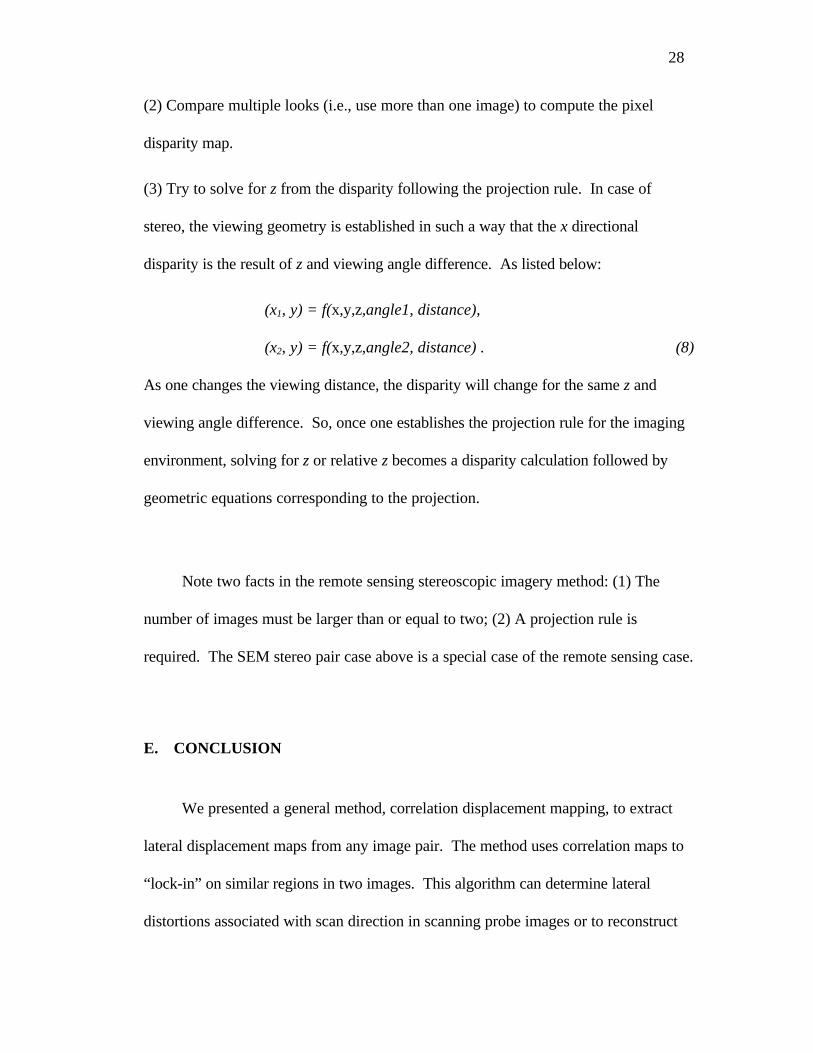
Figure II-1. (a) Schematic illustration of mapping algorithm. (b) An alternate kind of

image distortion might involve regional rotations. The algorithm examines two regions

from images A and B, respectively, and calculates the correlation between the two

regions. The higher the correlation coefficient is, the more alike the two regions are.

The lateral displacement is the center shift of these two regions. Although rotational

correlation functions might be used analogously for this task, the calculations done here

do not test for this kind of distortion. Rotational displacement is an option in the

displacement program.

(a)

(b)

31

Distortion source DX(displacement map DX)

Distortion source DY(displacement map DY)

Image A Image B

Autocorrelationmapping of A & B

CalculatedDisplacement mapsdx and dy

Recovered imagesfrom image pairs(A, dx) and (B, dy)

Original image: O (Starting image)

Figure II-2. The flow chart of the computer simulation. The grayed area in this chart is

what we did in actual experiments. Since we have knowledge of distortion sources DX

and DY, we can compare them with the calculated distortion sources dx and dy to see

whether or not the algorithm works.

32

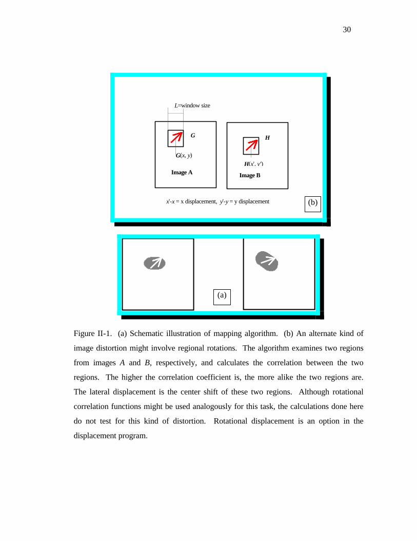
Figure II-3. The original (undistorted) image for the computer simulation. This is a

picture of the earth taken from a satellite. A grid and noise are superimposed on the

image. The grid is for the comparison and the noise is for texture enhancement. The

texture is the fingerprint needed for the correlation mapping algorithm to lock in the

pixel position.

33

Figure II-4. X direction distortion source (map). The grey value is the amount of the

distortion which will be imposed to the x direction of the original image. For example, if

the grey value is 9.90 at position (0,0), then the pixel of the original image at (0,0) will

be shifted 9.90 pixels in the x direction. This is the known distortion source which will

be compared to the calculated one from the correlation mapping.

34

Figure II-5. Y direction distortion source. The grey value of this image works the same

way as in Figure II-4, the X direction source, but in the y direction. The distortion will

be imposed in the y direction, not the x direction. In order to distinguish this from the X

distortion source, there are three periodical structures instead of four in Figure II-4.

35

Figure II-6. Image A, the first distorted image of an "experimental" image pair. This is

the distorted image in the x direction. If we have no knowledge of the object nor grid

lines, we would not know whether it is distorted or what the distortion source looks like.

36

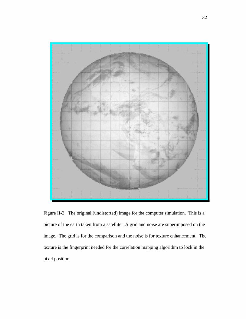
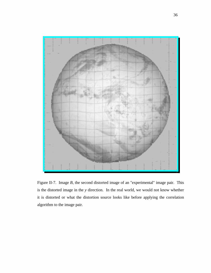
Figure II-7. Image B, the second distorted image of an "experimental" image pair. This

is the distorted image in the y direction. In the real world, we would not know whether

it is distorted or what the distortion source looks like before applying the correlation

algorithm to the image pair.

37

Figure II-8. Inferred or estimated x-direction displacement map. This is the calculated x

component of distortion source by correlation displacement mapping. We can see that it

is very similar to the X distortion source in Figure II-4. This proves that the algorithm

works for this case.

38

Figure II-9. Inferred or estimated y-direction displacement map. This is the calculated y

distortion component by correlation displacement mapping. It has three periodic

structures at both sides similar to Figure II-5. The major topographic structures of this

image and Figure II-5 are the same. Again this proves that the algorithm works for this

case. Note that we got gray edges because the mapping process needs a certain free

region (window) to perform correlation mapping.

39

Figure II-10. Image inferred by removing the estimated x-displacement. This is the

image recovered from Figure II-6, image A. It is obtained by correcting the image

Figure II-6 with calculated distortion map Figure II-8. Note the positions marked with

‘a’, ‘b’, ‘c’ and ‘d’ are not recovered very well compared with the center region. This is

due to the flat, grey region around the edge of Figure II-8.

c

a

bd

40

Figure II-11. Image inferred by removing the estimated y-displacement. This is the

image recovered from Figure II-7, image B. It is obtained by correcting the image

Figure II-7 with calculated distortion source Figure II-9. Note that the positions marked

with ‘a’, ‘b’, ‘c’, and ‘d’ are not recovered very well compared with the center region

due to the flat region around the edge of Figure II-9.

b

c

d

a

41

Figure II-12. The first image of a pair of scanning electron microscope images (image

A). This image was taken without tilting. The image was digitized from a photo. The

original image was of size 700×440 pixels. We cut a 440×440 portion from the original

and re-sized it to an image of 512×512 pixels. Thus the real resolution is 440×440

pixels. This image and the next one are from an advanced industrial laboratory.

42

Figure II-13. The second image of a pair of scanning electron microscopy images (image

B). This image was taken by tilting the sample at a small angle (about 5 degrees). Other

conditions were the same as Figure II-12 (image A) including the resolution.

43

project view from y

y

x

z, e-beam

EM-field aslens system

tilt angle x

z

αα

Sample

Figure II-14. A Schematic illustration of an equivalent optical system of scanning

electron microscope. The electromagnetic field works like an optical lens to the electron

beam. The drawing shows that the sample is tilted at a small angle (from the project

view at -y direction).

44

α

H

So

Xo

Sample

r r'α

Tiltedsample

x

y

z

Viewing direction

The sample before tilted.It is a board with an arrow

The sample after tilted byan angle α.

α

xy

Figure II-15. A schematic illustration of the relation between tilted and untilted samples.

H is the sample elevation at position (Xo, Yo). We do not see Yo here since this is a

projected view from the Y direction. The tilted angle is α. Sample center is at So on Z-

axis. After the sample being tilted, there is a lateral displacement (r’-r) in the X

45

direction. Here r and r’ are the image positions of untilted and tilted samples,

respectively.

Yo

H

rr'

So

Sample before tiltSample after tilt

y

zViewing direction

Figure II-16. A schematic illustration of the relation between tilted and untilted samples.

H is the sample elevation at position (Xo,Yo). Unlike Figure II-14, we do not see Xo here

since this is a projected view from the X direction. This angle causes the images of the

46

tilted and untilted samples to have a lateral displacement r’-r in the Y direction. The

sample center is at So on Z-axis.

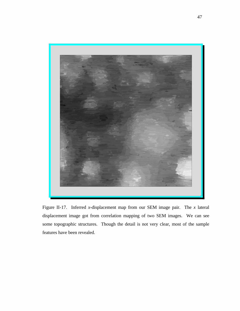
47

Figure II-17. Inferred x-displacement map from our SEM image pair. The x lateral

displacement image got from correlation mapping of two SEM images. We can see

some topographic structures. Though the detail is not very clear, most of the sample

features have been revealed.

48

Figure II-18. Inferred y-displacement map from our SEM image pair. The y lateral

displacement image derived from the correlation mapping of two SEM images.

According to the Equation (6), we can not see the topographic structures very clearly.

49

Figure II-19. Correlation coefficient map for our SEM image pair. The grey value is the

correlation coefficient. The larger the gray value, the more the two regions are alike.

50

Figure II-20. The image of optimized window size of mapping. The gray value is the

size of the mapping region. The smaller the gray values, the better the mapping

algorithm locks in on a location.

51

Figure II-21. Geophysics stereo pair mapping--remote sensing. The picture at the top is

the three-dimensional image and the one at the bottom is the two dimensional image with

user-added marks. (Magellan Stereo Experiment. F. W. Leberl et al., J. of Geophysical

Research, Vol 97, No. E8 (1992), page 13675.)

52

List I

The part of the code used to make a pair of images. It uses the displacement

maps to dislocate the starting image in order to distort the start image.

calculate x + fg2 to im1

calculate y to im2

stack im1, im2 to im3

reclass im3 plist

extract fg1 with im3 to fg4

calculate x to im1

calculate y+fg3 to im2

stack im1, im2 to im3

reclass im3 plist

extract fg1 with im3 to fg5

53

List II

The part of the code used to recover the distorted image. It uses the calculated

displacement maps to relocate the image in order to recover the distortion.

calculate x - fg6 to im1

calculate y to im2

stack im1, im2 to im3

reclass im3 plist

extract fg4 with im3 to fg8

calculate x to im1

copy y - fg7 to im2

stack im1, im2 to im3

reclass im3 plist

extract fg5 with im3 to fg9

54

III. LATERAL DISPLACEMENT MAPPING OF SCANNED PROBE

MICROSCOPE IMAGE PAIRS

A. INTRODUCTION

In this chapter, we study the lateral displacement caused by a scanning probe

microscope’s tip (i.e. lateral displacement maps) using the correlation-based lateral

displacement mapping technique discussed in Chapter 2. Tip displacement is one of

the distortions resulting from the interaction between tip and specimen, which is

found in scanning probe microscope images. The distortion is specimen dependent

and could provide information on sample surfaces. We describe a scanning tunneling

microscope experiment involving the lateral displacement mapping of a metal-coated

polymer hologram. The data show that the lateral displacement map has a spatial

frequency that is just double the frequency of sample topographic undulations. We

also examine lateral displacement maps taken with a contact-mode scanning (or

“atomic”) force microscope.

Distortions and artifacts in scanned probe microscope images are an important

issue in analyzing and understanding images. For example, specimen-dependent

“deviations from topography” found in scanning probe images can hardly be avoided.

55

We here examine one of many ways they provide interesting information on the tip-

sample interaction, namely on the mechanical interaction between tips and samples. It

will help us understand friction forces on the nanoscale as well. By studying lateral

displacement maps, we will be able to separate the lateral friction force from the

topographic component.

B. METHODOLOGY

In order to study the friction force in SPM, we could change the contact force

magnitude used as a set point for the feedback loop. Since the friction force is likely

opposite to the direction of motion, the simplest way to sense the friction force is to

vary the moving direction. Reversing the direction of the tip’s motion is one of the

simplest perturbations for studying the friction force in SPM. We might thus change

the scan direction, and study the differences between the image pairs. The difference,

in the form of lateral displacement vector map, provides us with information on the

friction coefficient. We expect that the friction-force related distortion to be the

opposite of the scan direction. Since the tip will be displaced by such a friction force,

there will be local displacement of high transverse-friction regions with respect to low

transverse-friction regions. Thus, we can study the friction by studying the lateral

displacement.

56

In contrast to non-mechanical microscopes such as far field electron

microscope, there is a direct local interaction between the sample surface and the

probe due to the nature of SPM. This is true even in the tapping-mode atomic force

microscope (TM-AFM), an instrument designed for “minimal-contact” imaging.

Hence there are numerous kinds of distortions and artifacts associated with tip-sample

interaction. Most of them are related to tip shape, surface topographic structure, and

surface contamination. In order to correctly interpret the SPM data, it is important to

catalog, to filter out and even, if possible, to utilize those distortions and artifacts

caused by SPM. Thus we might be able to collect important information from them

and to provide another way for understanding the specimen.

Some kinds of distortions of SPM are related to strong tip-sample interaction.

One example is the tip’s displacement due to the friction force between tip and

specimen. Although modern scanning tunneling microscopes (STM) have atomic scale

resolution, the tip displacement associated with lateral forces between specimen and tip

might be large (e.g., micron size) and specimen dependent especially for the sharp,

small cone angle tip. Things might be worse on soft samples in air-based scanning

tunneling microscopy and scanning force microscopy (SFM). We have observed that a

chemically-etched Au tip with a long tip head and very small cone angle is not able to

scan the sample surface, since the bending of the tip is so large that the displacement

57

exceeds the scan range. Thus it is standard practice to use hard materials such as

tungsten for sharp, small cone angle tips.

Generally, advantages and disadvantages of scanning probe microscopes come

from the same cause. The interaction between tip and sample will cause distortion and

artifacts, and then require image processing to correct them. But the very same

interaction also makes the microscope capable of nanoscale manipulation, and provides

vital information on the specimen surface.

An advantage of using lateral displacement maps to study friction force in this

way is that it is experimentally simple. Special hardware is not needed, only the usual

ability to change scan direction! As we show in the next chapter, the approach also

de-couples the friction force from the sample surface topography. This technique

allows simultaneous measurement of both x and y components of the drag-related

displacement, and no topographic terms complicate the lateral displacement map’s

proportionality to the magnitude of the friction force. Absolute measurements of

lateral forces, such as those obtained by cantilever twists from commercial AFM,

require extra hardware only available for scanning-cantilever systems, provide a signal

which may be dominated by purely geometric effects (i.e. by surface topography

alone), and can not measure the lateral force in two directions simultaneously.

58

C. IMAGE PAIR ACQUISITION

The specimens for this study are holograms coated with copper. The imaging

systems we used are the NanoScope I and NanoScope III Microscopes from Digital

Instruments. We wrote our own data acquisition program for an IBM PC, which is

dedicated to tip control and data acquisition with the NanoScope I. While on the

NanoScope III, we took lateral force images in contact LFM and AFM modes. We

prepared Pt/Ir tips by an acid etching technique. The LFM cantilever was specified by

Digital Instruments as having a 100-nm wide leg with a spring constant of 0.58 N/m.

STM images were acquired with a Digital Instruments' air-based NanoScope I (helical

scan as well as raster scan) and AFM and LFM images with a Digital Instruments’

NanoScope III (raster scan only). STM images were acquired under constant current

mode with 40 mV bias voltage and 2 nA tunneling current. Scan speed is set at 5 Hz for

512×512 pixels image of less than 10 microns size view.

There are several considerations in the choice of parameter settings. Changing

the bias voltage and tunneling current will change the height of the probe from the

surface and, hence, change the friction force. The further the tip is away from the

surface, the less the friction force. The friction force is also effected by the travel

speed of the tip in the adsorbed surface-layer on the specimen. In order to reduce the

effect of scan speed, a slow scan is required to study the normal and friction forces.

Scanning at a speed below 5 Hz/line for a 512×512 pixels image of a 10 µm by 10 µm

59

size area (at the speed lower than 50 microns/second) satisfies this requirement. If the

speed is faster than 100 microns/second, we did not see clear lateral displacement

features. Since the tip may change the sample surface especially in contact mode

scanning force images, the effects of the physical changes of tip and specimen also

have to be considered.

The images shown as Figure III-1 and Figure III-2 are a pair of clockwise-

counterclockwise helical scanned images. Those distorted clockwise-

counterclockwise helical scan STM images of the hologram show lateral tip

displacements on the order of 0.5 µm. This is the first time we have evidence that the

image is distorted by the tips’ bending and the distortion is related to scan direction

and sample topographic structure.

Figure III-3 and Figure III-4 are a pair of left-right raster scan STM images of a

hologram sample. There are about five and half spatial gratings in the image. The

wavelength is about 2 microns. Compared to the left scan image, the right scan image

shifts to the right by about half of wavelength, or about one micron. The difference

between the left and right scan images does not directly show any interesting

microscopic features except for this left-right shift of about a half-column of the

corrugated structure. Also, there are a few defects caused by an imperfect feedback

loop response, such as the “flying line”. These minor defects did not effect our results.

AFM and LFM images on holograms show differences in comparison to the STM

images (please refer to Figure III-12, Figure III-13, and Figure III-15 for AFM and

LFM images). There is also a double spatial frequency feature found comparing AFM

60

with LFM images (Figure III-14). However, there are a set of secondary-minimum

data and a set of sub-maximum ones, etc., marked as ‘MIN’, ‘MAX’, ‘A’, ‘B’, and

‘C’.

D. ANALYSIS AND RESULTS OF STM IMAGE PAIR

The algorithm described in Chapter 2 was used to extract lateral displacement

maps from our two three-dimensional STM images of the hologram. After the lateral

displacement map was obtained, it was also possible to remove such lateral distortion

from the original images. For simplicity, we interpret the gray value in STM images

as the height of the specimen and use it as the fingerprint for the mapping. The lateral

displacement vector is stored in two image files, namely X (Figure III-5) and Y

(Figure III-6), for x and y displacement components, respectively.

Only in image X, we observe a sinusoidal feature which has a spatial periodicity

whose frequency is double that of the periodicity found in the specimen’s topography

(Figure III-3 and Figure III-5). More importantly, when we examined sinusoidal

structures of the specimen and the X image, we find that the minimum value of image X

appears on the slope regions of the specimen, and the maximum value appears on the

mountain and valley regions, respectively. The largest displacement happens in regions

where the surface is flat. This is very clear when we project the specimen image and

the x-displacement map orthogonal to the direction of specimen periodicity, i.e., along

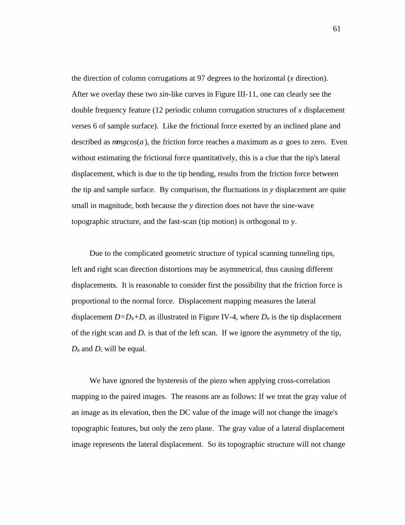
61

the direction of column corrugations at 97 degrees to the horizontal (x direction).

After we overlay these two sin-like curves in Figure III-11, one can clearly see the

double frequency feature (12 periodic column corrugation structures of x displacement

verses 6 of sample surface). Like the frictional force exerted by an inclined plane and

described as µmgcos(α), the friction force reaches a maximum as α goes to zero. Even

without estimating the frictional force quantitatively, this is a clue that the tip's lateral

displacement, which is due to the tip bending, results from the friction force between

the tip and sample surface. By comparison, the fluctuations in y displacement are quite

small in magnitude, both because the y direction does not have the sine-wave

topographic structure, and the fast-scan (tip motion) is orthogonal to y.

Due to the complicated geometric structure of typical scanning tunneling tips,

left and right scan direction distortions may be asymmetrical, thus causing different

displacements. It is reasonable to consider first the possibility that the friction force is

proportional to the normal force. Displacement mapping measures the lateral

displacement D=DR+DL as illustrated in Figure IV-4, where DR is the tip displacement

of the right scan and DL is that of the left scan. If we ignore the asymmetry of the tip,

DR and DL will be equal.

We have ignored the hysteresis of the piezo when applying cross-correlation

mapping to the paired images. The reasons are as follows: If we treat the gray value of

an image as its elevation, then the DC value of the image will not change the image's

topographic features, but only the zero plane. The gray value of a lateral displacement

image represents the lateral displacement. So its topographic structure will not change

62

if we add a DC constant displacement value to its gray value. In our experiment, if the

hysteresis is introduced by changing the direction of raster voltage, then the hysteresis

only adds a constant gray value to the whole image.

Since the SPM piezo-electric crystal is scanning in both x and y directions,

hysteresis effects are unlike to be confined to one directions. What is more, the

displacement due to the piezo's hysteresis is not likely to oscillate repeatedly along any

scan direction. If the value of hysteresis of the piezo changes gradually along the

scanning path, it only adds a slowly changing background to the X-displacement image.

If the hysteresis is a function of x and y, it is not likely to have a sinusoidal profile when

it is projected orthogonal to the direction of the periodicity. When we project them to

110 degrees, all the sinusoidal features, as well as the double frequency feature, are

gone! Thus the discussed features are not caused by the hysteresis.

E. LFM IMAGES OF HOLOGRAM

Lateral displacement maps measure changes in the tip’s bending between scans,

and hence measures lateral components of both friction and the normal force. It is

interesting to compare lateral displacement maps with lateral force (LFM) images

obtained with the AFM. In our LFM image of the hologram (Figure III-12 and

Figure III-14), the lateral force reaches its largest value in the valley areas and its

smallest values on slopes. The twist of the cantilever in mountain areas is bigger than

the twist of the cantilever in slope regions. If we directly examine the image from the

top view, the evidence of double frequency is unclear. After we project the image to

63

128 degrees from the horizontal direction, the double frequency feature becomes

easily visible (Figure III-14).

In comparing lateral displacement maps to lateral force images, we see that the

LFM hologram image has a set of sub-maximum points. Those points are due to either

the difference in roughness at trough and mountain areas, or to a thicker contamination

layer in the trough region. Notice that there is also a set of secondary-minimum

points. One possible explanation of the secondary-minima is that LFM lateral force

microscopy also takes the normal force into account. On uphill traveling, the torque

acting on the cantilever is larger than that during downhill traveling on the surface

regions with same tilt angle. Therefore, there is a set of secondary-minimum points.

The fact that the STM x displacement image has the double frequency structure,

and the y displacement does not, gives us a clue that the tip’s displacement has a

strong connection to the scan path and geometric structure along the path. The

difference between LFM images and STM lateral displacement maps prompts us to

look into the contrast mechanisms in such images. In the next chapter we will present

some models and provide an explanation of the data.

F. CONCLUSION AND SUMMARY

We applied the method of lateral cross-correlation mapping to study pair

scanning STM images on holograms. We compared these lateral displacement maps

with AFM and LFM images. The data shows that there is a double spatial frequency in

64

an STM’s lateral displacement maps, as well as in LFM images. There are differences

between the double spatial frequencies of STM images and LFM images, such as the

asymmetrical double frequency in LFM. The relation of lateral displacement maps,

LFM images, and the feed back loops of STM and LFM need to be studied. The

double-frequency features in the lateral displacement maps hint that the lateral

displacement of the tip is very likely related to a frictional force. It needs further

theoretical study, and a model is needed to explain the data.

65

Figure III-1. Clockwise (CW) outward helical scan STM image of a hologram. A

cross locates the helical center. The field of view is about 5 microns. The

displacement is above a half micron at the edge area, when comparing CW and CCW

images. The bending of the tip causes such distortion.

66

Figure III-2. Counter-clockwise (CCW) outward helical scan STM images of a

hologram. The cross locates the helical center. The field view is about 5 microns. The

displacement is above a half micron at the edge, comparing the CW and CCW images.

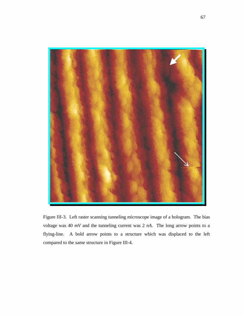
67

Figure III-3. Left raster scanning tunneling microscope image of a hologram. The bias

voltage was 40 mV and the tunneling current was 2 nA. The long arrow points to a

flying-line. A bold arrow points to a structure which was displaced to the left

compared to the same structure in Figure III-4.

68

Figure III-4. Right raster scanning tunneling microscope image of a hologram. The

parameter setting is the same as Figure III-3. The bias voltage was 40 mV and the

tunneling current was 2 nA. We can see a dent being displaced to the right (an arrow

points to the same structure in Figure III-3).

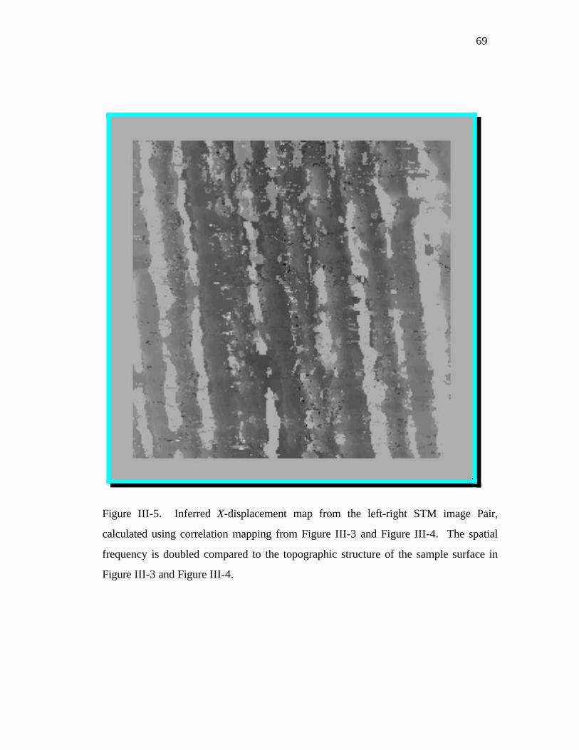
69

Figure III-5. Inferred X-displacement map from the left-right STM image Pair,

calculated using correlation mapping from Figure III-3 and Figure III-4. The spatial

frequency is doubled compared to the topographic structure of the sample surface in

Figure III-3 and Figure III-4.

70

Figure III-6. Inferred Y-displacement map from the left-right STM image. There is no

periodic structure. We can see no interesting patterns in this image.

71

Figure III-7. A correlation coefficient map obtained from the left-right STM image

Pair. The grey value of the image is the largest coefficient in the cross-correlation

integral. The higher the grey value is (i.e. the brighter the image), the better the

algorithm can lock in the position. Please refer to Figure III-8 for a more detailed

explanation.

72

Figure III-8. A map of the window size which gave the best off-set value for

correlation coefficient. The gray value of the image is the base 2 logarithm of mapping

window size (in pixels on a side). Generally, the lower the gray value is (i.e. the darker

the image), the better the mapping algorithm can lock in the position. If the sample is

very rough and noisy, bigger window sizes may produce better correlation coefficients.

73

Figure III-9. Projected view of X displacement image. This is the projection of Figure

III-5 in a direction 97.5 degrees from the x-axis. This direction is that of the

periodicity in the hologram sample. We can see that this is a periodic curve. The two

flat ends are due to the grey edge of the Figure III-5. MEAN=-5.74 and SD=5.68

74

Figure III-10. Projected view of y-displacement in the left-right STM image pair. Same

as in Figure III-9, a projection of Figure III-6 at 97.5 degrees in the direction of sample

periodicity. The MEAN = 0.33 pixels and SD= 0.88, much smaller than that of X

displacement image. There is no interesting pattern of Y displacement image.

Project view of Y-displacement image

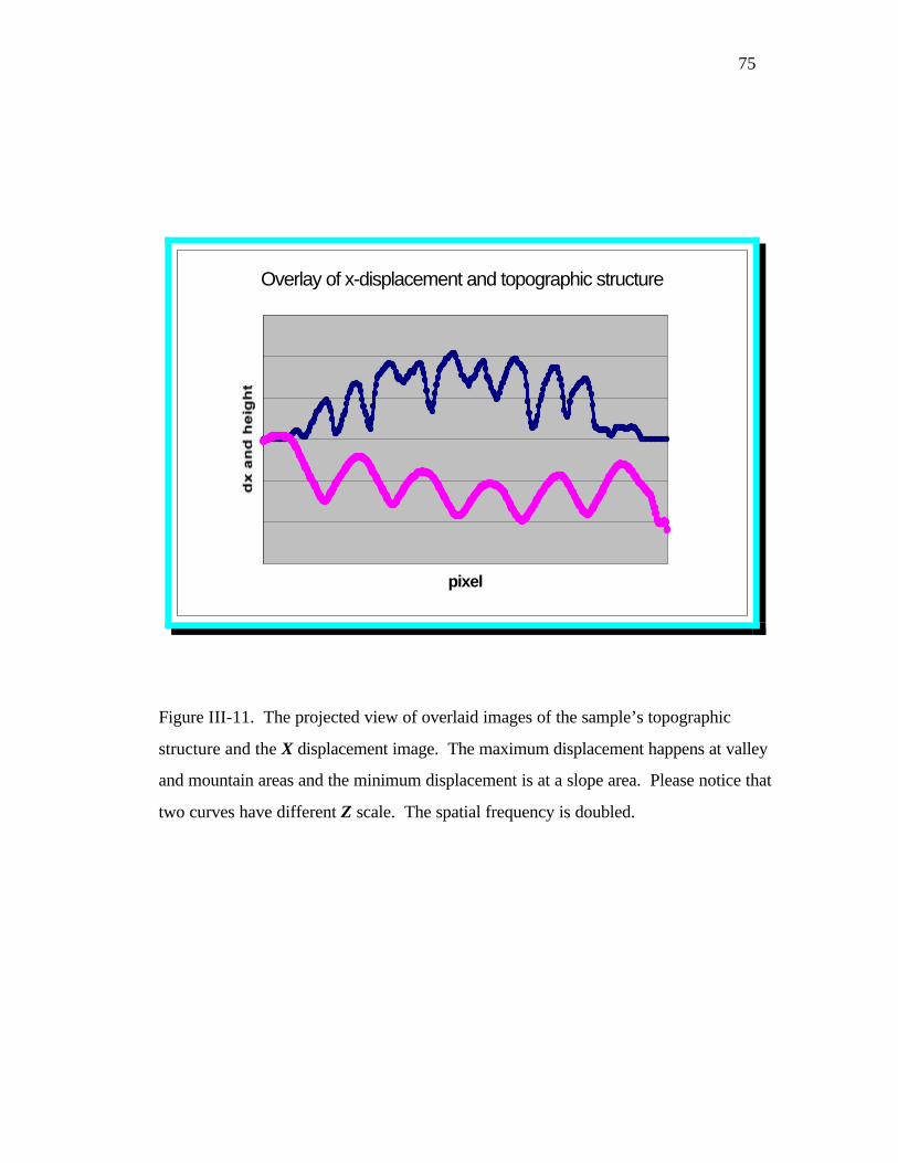
75

Overlay of x-displacement and topographic structure

pixel

Figure III-11. The projected view of overlaid images of the sample’s topographic

structure and the X displacement image. The maximum displacement happens at valley

and mountain areas and the minimum displacement is at a slope area. Please notice that

two curves have different Z scale. The spatial frequency is doubled.

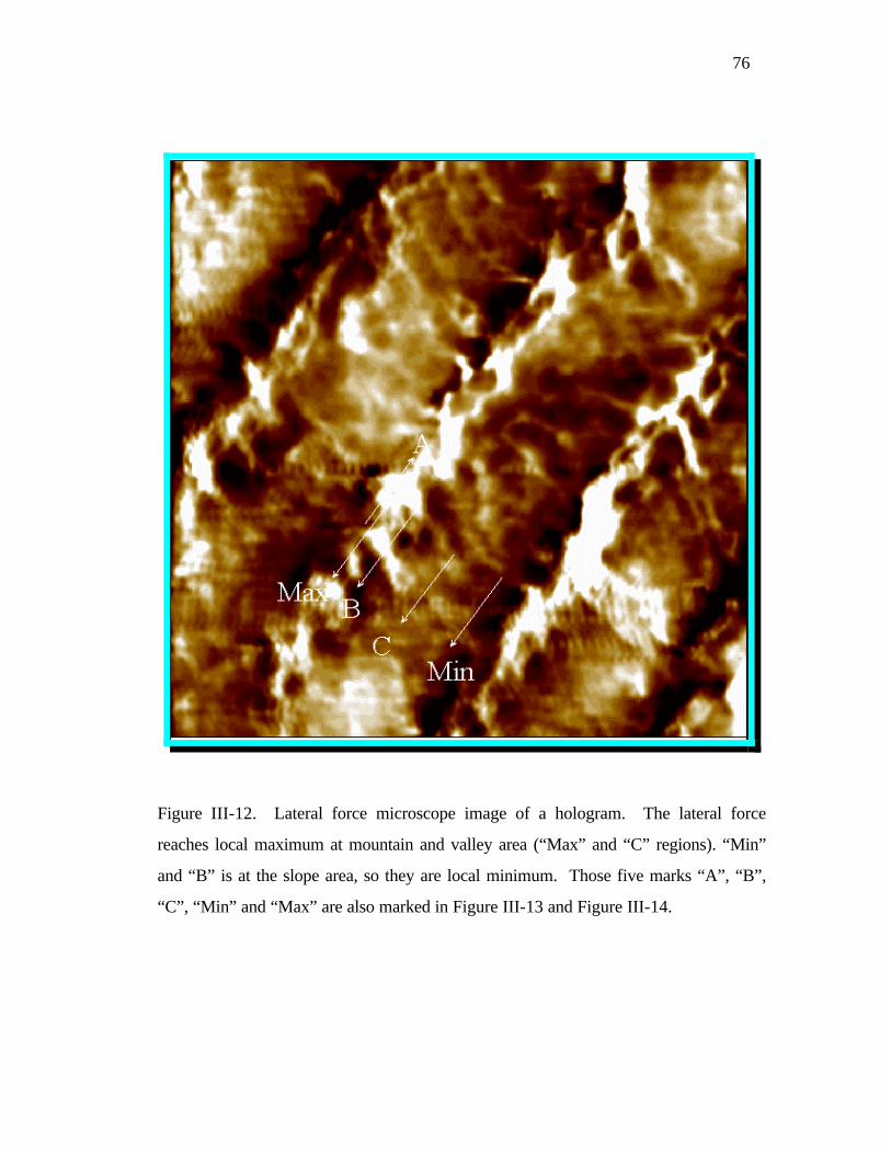
76

Figure III-12. Lateral force microscope image of a hologram. The lateral force

reaches local maximum at mountain and valley area (“Max” and “C” regions). “Min”

and “B” is at the slope area, so they are local minimum. Those five marks “A”, “B”,

“C”, “Min” and “Max” are also marked in Figure III-13 and Figure III-14.

77

Figure III-13. Contact-Mode scanning force height image of the hologram in the same

region as Figure III-12. The mark “Max”, “A”, “B”, “C”, and “Min” are explained in

Figure III-15.

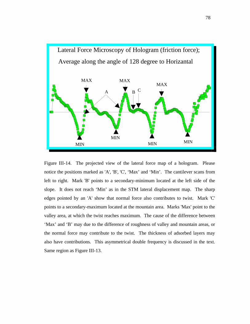
78

Lateral Force Microscopy of Hologram (friction force);

Average along the angle of 128 degree to Horizantal

MIN

MINMIN MIN

MAX MAXMAX

A B C

Figure III-14. The projected view of the lateral force map of a hologram. Please

notice the positions marked as 'A', 'B', 'C', ‘Max’ and ‘Min’. The cantilever scans from

left to right. Mark 'B' points to a secondary-minimum located at the left side of the

slope. It does not reach ‘Min’ as in the STM lateral displacement map. The sharp

edges pointed by an 'A' show that normal force also contributes to twist. Mark 'C'

points to a secondary-maximum located at the mountain area. Marks 'Max' point to the

valley area, at which the twist reaches maximum. The cause of the difference between

‘Max’ and ‘B’ may due to the difference of roughness of valley and mountain areas, or

the normal force may contribute to the twist. The thickness of adsorbed layers may

also have contributions. This asymmetrical double frequency is discussed in the text.

Same region as Figure III-13.

79

Figure III-15. The overlay image of lateral force image and height image (Figure III-12 and Figure III-13).

80

IV. THEORY OF THE DDOUBLED SPATIAL FREQUENCY IN

HOLOGRAM STM LATERAL DISPLACEMENT MAPS

A. INTRODUCTION

In the previous chapter, a “double spatial frequency” structure in lateral

displacement maps obtained from STM hologram images was described. In this

chapter, we present a possible explanation for this double spatial frequency. We will

also discuss the differences between lateral displacement microscope images and the

lateral force microscope images.

Our discussion of lateral displacement is in the framework of Newtonian

mechanics. Elastic deformation of the sample and the tip, the tip's shape, and the

surface layer adsorbed on any surface in air all make contributions to observed

lateral displacement maps. Because the effects observed are larger than the

coherence distance for atom-bound electrons, Newtonian mechanics is appropriate.

This approach should work for other lower resolution SPM images as well.

81

B. THEORY OF LATERAL DISPLACEMENT MAPS - SCANNING

TUNNELING

In air-based scanning tunneling microscopy, mechanical forces are known to

exist between the tip and specimen. The normal force N, and the friction force f, are

surface slope shown in Figure IV-1 and Figure IV-2 (with α between -ππ/2 to +ππ/2

radians). Since the current between specimen and tip is held constant by the feedback

loop, one might guess that the normal force N between specimen and tip is to the first

order constant as well. The vertical (V) and lateral (L) components of those

specimen forces, which of course the microscope must balance if the tip is to remain

unaccelerated, then become

)( )(= αα sincos f N V m± (9)

).( )( = αα cossin fNL ±± (10)

Here the top/bottom subscripts are for (fast) scans in the positive and negative

directions, respectively. Note that the lateral force has a geometric component,

sin(α), which is independent of scan direction, and present even in the absence of

friction. Variations in cos(α) dominate only when the friction force f is larger than

the normal force N. Hence, when the coefficient of friction µ= f/N is small or

relatively constant from point to point, one expects lateral force images to be

dominated by topographic contrast.

82

The following mechanism can account for the doubled spatial frequency of

lateral displacement maps. Suppose that the following two conditions are true: (1)

The lateral displacement in a given image is proportional to the lateral force and (2)

Reversing the scan direction simply reverses the direction of the friction force while

leaving the normal force unchanged. Then from Equation (10), the change in the

lateral displacement between two images taken with the scan direction reversed will

be proportional to

)cos(αδ fLLL 2≅−≅ −+ . (11)

The approximation sign is used because the friction force and the normal force for

different scan directions may not be identical in real situations. The Nsin(α) terms

subtract out. Hence, the amount of lateral displacement between two images taken

with opposite scan directions, unlike the lateral force itself, is simply proportional to

the magnitude of the friction force between specimen and tip. No friction force

means no contrast in the image. Lateral displacement images will show topographic

variation through the cos(α) factor, although when α is small (i.e., for relatively flat

specimens), any significant changes in the friction force from point to point will likely

dominate the contrast.

Topographic structure in the lateral displacement, i.e., the cos(α) factor, is an

even function of α which reaches a maximum when α is zero (the surface is flat)

83

and reaches a minimum when α goes to its positive and negative extrema. Let’s

look at an example of a surface which has the topographic structure, e.g. S(x)=A

sin(2πx/λ). The function of α is then

α(x)=tan-1[2πA /λcos(2πx/λ)], (12)

and the lateral displacement is

L(x)≅2fcos{tan-1[2πΑΑ/λcos(2πx/λ)]}. (13)

This is of course the half-wavelength or "double frequency" function that we saw in

the lateral displacement image of the STM hologram image! The plot of those

functions S(x), α(x), dS(x)/dx, and L(x) are shown in Figure IV-3.

C. THEORY OF LATERAL DISPLACEMENT MAPS - SCANNING

FORCE

In scanning force microscopy, the feedback loop is typically designed to hold

a constant vertical force between specimen and tip. In the case of repulsive

(contact-mode) scanning force microscopy (AFM or SFM), if we assume that to the

first order the feedback loop holds a constant vertical force V between specimen

and tip, then the normal force N from Equation (9) is

)sin()cos( αµα −=

VN

, (14)

84

where we again define the coefficient of friction as µ. If the absolute value of α is

small enough so that the required normal force does not cause appreciable specimen

deformation, the lateral force becomes

)sin()cos(

)cos()sin(

αµααµα

−+

= VL.

(15)

The denominator of this equation goes to zero for α when

)(tan µαα 11−== o . (16)

Hence, for constant V, the lateral force is a monotone function of α except at the

singularity αo. Separate minima for positive and negative values of α do not occur,

and a "double-frequency" pattern of the sort seen with the displacement image above

is not expected.

As before, if lateral displacement is proportional to lateral force, and if

reversing the scan direction simply reverses the direction of the friction force while

leaving the normal force unchanged, then the change in lateral displacement

between two images taken with the scan direction reversed will be proportional to

)(sin)(cos αµαµ

δ222

2

−=−= −+

VLLL

. (17)

This is symmetric about α=0 as in the constant normal force case, although it has a

central minimum (of 2µV) rather than a maximum. Thus, again in the displacement

85

image, we expect a double frequency effect, albeit one which is inverted in

comparison to the constant normal force case.

In our force microscope, the cantilever deflects an angle φ when the tip is

traveling. The LFM measures this twist angle φ, and hence measures the combination

of normal force N and friction force f. Let us still assume that f is proportional to

normal force N and f=µΝ. Under conditions of constant vertical force, the combined

force on the cantilever should balance the torque of the twist cantilever. A vector

calculation leads us to

)sin()cos(

)sin()cos(

αµαφαφαµ

−+++

= VT.

(18)

Notice that it has a singularity, as does Equation (16). The torque balance does not

introduce any new physics. When α→ αο, the normal force Ν→∞. In practice, when

α exceeds a critical value, say αmax, the normal force will be so large that the sample

surface can no longer bear it. The surface forms a dent to hold the tip in order to

change the direction of the normal force until the condition of constant vertical force

returns. The critical angle αmax is given by Equation (19). We include surface

deformation from Equation (16) to give

maxmax ),(tan

NV

=−

−+−= − ξ

ξµξµξµ

α22

221 1

(19)

86

>=≤=

max

max

),/(

,

αααααααααα

(20)

where Nmax is the maximum normal force that the sample surface can bear. Equation

(20) sets a limitation of αmax ≤ αο. So α always reaches αmax first and then surface

deformation occurs. The singularity is thus avoided. We might be able to verify the

existence of αmax by increasing sample's tilt angle when we are imaging the force

curve with zero scan size.

Equation (18) shows that the torque acting on the uphill traveling (α>0)

cantilever is larger than the one acting during downhill travel (α<0), though φ is

very small (less than one degree). When α>>φ and α>45 degrees, the lateral

displacement is mainly determined by the topographic structure of the sample

surface or the topographic factor α. In the case of α<<1 and φ<<1, the surface is

flat and the twist angle of the cantilever is approximately proportional to

T/V = µ (1+α2 )+ α (1+µ2 ) ≈ µ. (21)

Only in this case does LFM measure the friction coefficient on the sample surface.

Usually LFM measures a combination of friction coefficient µ and topographic

structure α. It is interesting that we might be able to convert an AFM topographic

image (which is converted to an α-value image) and an LFM image (the torque image

87

which is proportional to T) to a friction coefficient image with the help of Equation

(21).

Our first attempt to verify these relationships in scanning force microscopy

has resulted in a puzzle and a need for further work. Unfortunately, the LFM image

has a double frequency structure which is not reversed, as predicted by Equation (9)

and Equation (17). The image in Figure III-14 is a profile of the lateral force

microscope image of our hologram, projected orthogonal to the direction of the

periodicity. Note that a double frequency feature is present, although it is non-

symmetric, as one might predict for a lateral force image taken under conditions of

constant normal force. Unfortunately, a constant repulsive feedback loop was in

operation, for which our simple model predicts no double minima.

This conflict between theory and experiment is currently under investigation.

For example, a model that considers the cantilever’s tilt angle φ during the scan might

help. Another possibility is that the high normal force and rounded contact areas of

cantilevers operating in the repulsive force mode (as compared to air-based scanning

tunneling tip operation) might require a different look at the physics altogether.

88

D. LATERAL DISPLACEMENT MAP MODELS

Since the experimental data shows differences between AFM and STM, we

can combine the two formulas for STM and AFM, forming a mathematical hybrid of

constant normal force and constant vertical force. Specimen hardness may play a

role in AFM displacement maps, but not in air based STM displacement maps.

For AFM, we assume that the feedback loop keeps some combination of

vertical and normal forces constant. This is reasonable since the twist torque and

the forces at x-y direction both need to be balanced. When the ratio of vertical to

normal force goes to zero, it is a pure constant vertical force model. When the ratio

reaches infinite, it is a constant normal force model. We analyze the simulated AFM

images on a cosine ripple of cos[|r|] (Figure IV-6). The images are calculated by

assuming that the specimen deforms if the normal force of the tip exceeds a critical

value. From the images Figure IV-7 to Figure IV-9, the simulation shows that

when the ratio rises from zero to one, the spatial frequency of lateral displacement

changes from no double frequency to non-symmetric double frequency, then to

symmetric one. Hence the observation of a non-symmetric double frequency in

LFM hologram images indicates that the feedback loop does not obey the pure

vertical force constant rule. (Note: It is better to say that the feedback loop does not

keep the vertical force 100% constant)

89

E. CONCLUSIONS AND SUMMARY

Lateral displacement maps from the STM hologram images show that there is a

doubled spatial frequency along the x direction. From a Newtonian model, the

doubled spatial frequency in these maps indicates that the lateral force primarily is a

friction force. The normal force (here the repulsive force between sample and tip)

between tip and the sample is approximately unchanged during the scanning process.

The deformation of samples, particularly soft samples, mixed with the deformation of

the tip, will make lateral displacement mapping more complicated. It would be

interesting if the tip's deformation can be ignored and the lateral displacement

significantly came from the deformation of the sample. In that case we might be able

to detect structure beneath the soft sample surface via our lateral displacement

calculations.

In LFM images, in addition to the double frequency feature, there are

secondary-maximum and secondary-minimum in the microscopy data. These

secondary-minimum are located on the sloped areas at each side of the hologram

column corrugations. We explain these secondary-minimum qualitatively by a model

which considers twists of the cantilever a function of both normal and frictional

forces. Uphill traveling will yield a larger twisting of the cantilever than downhill

90

traveling. According to this model, LFM measures a combination of friction

coefficient µ and topographic structure tangent angle α.

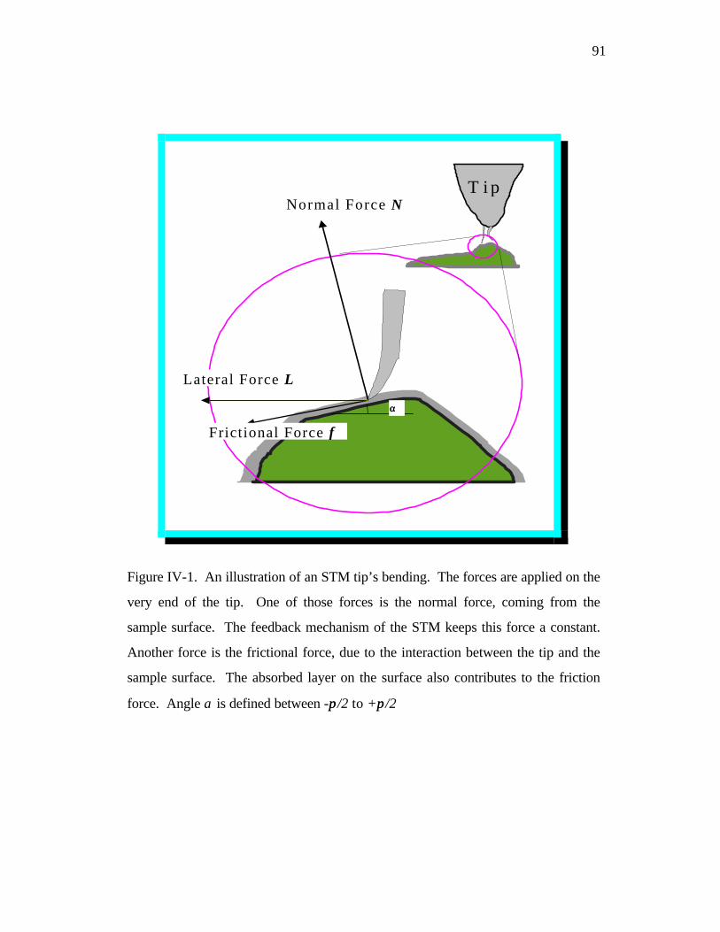
91

T i pNormal Force N

Lateral Force L

Frictional Force f

αα

Figure IV-1. An illustration of an STM tip’s bending. The forces are applied on the

very end of the tip. One of those forces is the normal force, coming from the

sample surface. The feedback mechanism of the STM keeps this force a constant.

Another force is the frictional force, due to the interaction between the tip and the

sample surface. The absorbed layer on the surface also contributes to the friction

force. Angle α is defined between -ππ/2 to +ππ/2

92

Normal Force N

Lateral Force L

Frictional Force f

T w ist force T

V e r tical F o r c e V

C a n ti lever

Figure IV-2. An illustration of the twist of the AFM cantilever. There are two

forces that have contributed to the torque. The combined effect is decided by

which balance mechanism the AFM uses. If the vertical force is kept constant,

down hill and up hill traveling will have different torque.

93

Surface and Lateral Force

dy/dx Lateral forceSurface y(x)

Figure IV-3. A classical example of constant normal force STM tip displacement.

A plot of the curves of S(x), α(x), dS(x)/dx and L(x) as predicted by Equation (12)

to Equation (13) are shown. We can see the double spatial frequency (half

wavelength).

94

Figure IV-4. The DR and DL of tip’s bending. The imaged feature is shifted left and

right respectively for the left and right raster scan.

Object X

Left scanned tip Right scanned tip

X moves to XR in right scannedimage

XR

X moves to XL in left scannedimage

XL

DL=|X-XL| DR=|X-XR|

DL DR

95

Figure IV-5. Up hill and down hill travelling cantilever will have different torque.

Due to combination of α and φ angles, the normal force, friction force and the

vertical force will have different contributions. Where α is the angle between

normal force and vertical force and φ is the angle of cantilever and vertical force.

The angle of α+φ is the angle between the torque and the surface.

Vertical force VNormal force N

Torque T

Friction force f

α+φ

α φ

T’

f’

V’N’

α’-φ’

α’

φ’

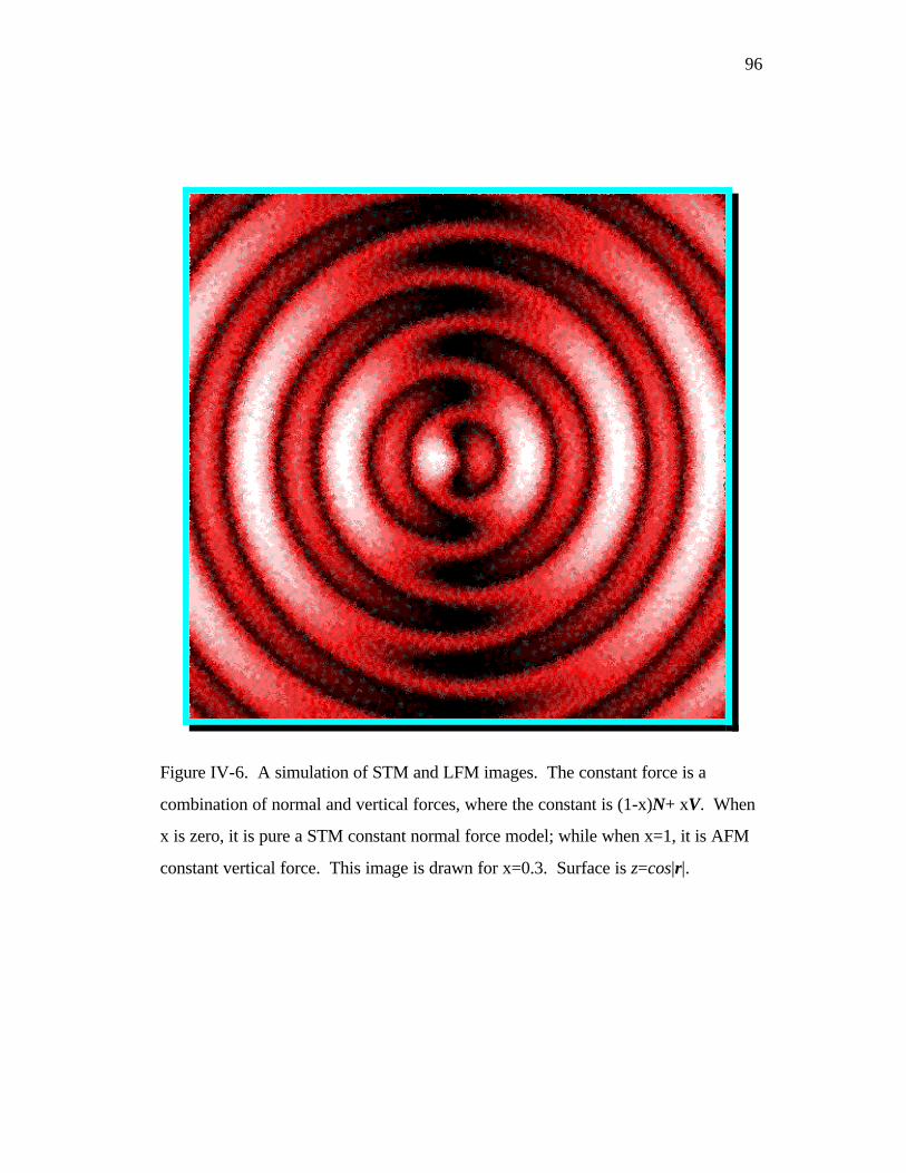
96

Figure IV-6. A simulation of STM and LFM images. The constant force is a

combination of normal and vertical forces, where the constant is (1-x)N+ xV. When

x is zero, it is pure a STM constant normal force model; while when x=1, it is AFM

constant vertical force. This image is drawn for x=0.3. Surface is z=cos|r|.

97

Figure IV-7. The relationship between the normal force and the surface tangent.

As the slope becomes deeper, the normal force becomes larger.

98

Figure IV-8. A three dimensional view of double frequency. Surface is z=cos|r|. It

simulates the tip scanning in the x direction. The friction is superimposed as color

onto the topographic surface. Friction increases as the color changes from green to

red.

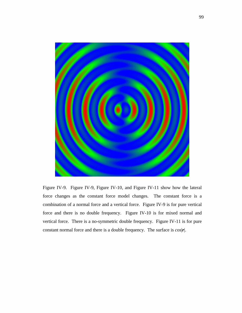
99

Figure IV-9. Figure IV-9, Figure IV-10, and Figure IV-11 show how the lateral

force changes as the constant force model changes. The constant force is a

combination of a normal force and a vertical force. Figure IV-9 is for pure vertical

force and there is no double frequency. Figure IV-10 is for mixed normal and

vertical force. There is a no-symmetric double frequency. Figure IV-11 is for pure

constant normal force and there is a double frequency. The surface is cos|r|.

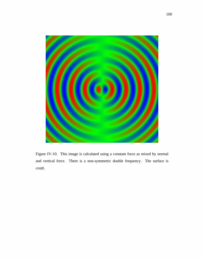
100

Figure IV-10. This image is calculated using a constant force as mixed by normal

and vertical force. There is a non-symmetric double frequency. The surface is

cos|r|.

101

Figure IV-11. This is a pure constant normal force case and there is a double

frequency

102

V. THE RELATIONSHIP BETWEEN A TIP’S BENDING AND

THE FORCE APPLIED

A. INTRODUCTION

In this chapter, we ask: Do the displacements reported in Chapter Three

result from lateral forces of plausible size and can we use lateral displacement

maps to obtain quantitative maps of the forces of lateral interaction? In order to

calculate the lateral force associated with a tip’s lateral displacement, we must

study the relationship between the bending of a tip and the force applied to it. In

this chapter, we take both analytic and numerical approaches. All are based on the

classic mechanical model of a bending beam.

B. CLASSICAL MODEL

Classical mechanics has a well-developed model for beam-bending, based on

Young’s theory95. In this chapter I treat the scanning probe tip as a classic beam.

The amount of tip displacement depends on the force F applied at the tip’s head

(the end nearest to the specimen), and the tip’s Young’s modulus E. The

103

displacement is very sensitive to tip shape and dimensions, e.g., the cone angle of a

conical tip.

Consider the segment of beam as shown in Figure V-1. The beam is bent by

a pair of forces F and -F. Suppose the length of a beam segment is L. The

change of the length of this segment, dL, is a function of the offset from its center

line, as:

dxR

rdxdrRdLL +=+=+ θ)( . (22)

Hence

dxR

rdL = . (23)

Here R is the radius of curvature and dθ is the angle shown in Figure V-1. From

Young’s theory, the force is proportional to E×dL. Thus the stress T (Force per

unit area) is proportional to the rate at which force increases as the segment length

dx is increased:

R

rE

dx

dLET == , (24)

where E is Young’s modulus for the material from which the beam is made. The

force then becomes

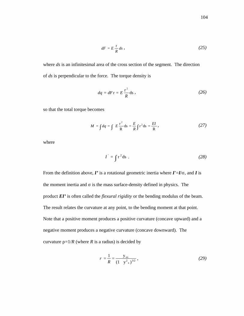
104

dsR

EdFr

= , (25)

where ds is an infinitesimal area of the cross section of the segment. The direction

of ds is perpendicular to the force. The torque density is

dsr

r2

REdFdq == , (26)

so that the total torque becomes

∫∫ ∫ ====R

dsrdsRr 2

2 EI

R

EEdqM , (27)

where

∫= dsr 2'I . (28)

From the definition above, I’ is a rotational geometric inertia where I’=I/σ, and I is

the moment inertia and σ is the mass surface-density defined in physics. The

product EI’ is often called the flexural rigidity or the bending modulus of the beam.

The result relates the curvature at any point, to the bending moment at that point.

Note that a positive moment produces a positive curvature (concave upward) and a

negative moment produces a negative curvature (concave downward). The

curvature ρ=1/R (where R is a radius) is decided by

3/2x

2xx

)y(1

y1

+==

Rρ , (29)

105

where we define yx ≡ dy/dx and yxx ≡d2y/dx2. After we discard the second order

infinitesimal, this becomes:

.dx

yd2

2'EIM = (30)

Now we obtain the basic relationship for determining the deflection curve. From

this solution we can obtain all the information needed, such as beam’s slope and the

deflection function. Note that

dx)dxx()x( FMM =+− . (31)

Hence,

3

3'

dx

ydEIF −= . (32)

The negative sign can be eliminated by redefining the direction of the stress T to -T.

Finally, this yields96, 97

'3

3

dx

yd

EI

F= . (33)

We first assume that the shape of a tip is cylindrically symmetric. Then, its

shape can be described by the radius function r(x) for its radius at lateral position x

106

r(x)r = . (34)

The following equation then shows a truncated form for this function r(x), which

models a conical tip:

1k0R(x),R)L

x)(Lk)(1(kRr(x) 0n

n

0 ≤≤=−

−+= . (35)

Here L is the total length of the tip, R0 and R1 = kR0 are the radii at x=0 and x=L,

respectively. The tip’s head (the end which is closer to the specimen) has radius

r(L)=R1. The tip shape as a function of power law index n and tip reduction ratio k

is shown in Figure V-8.

If the cross section of the tip is a circle, then the geometric inertia is

I’=(1/2)πr4. Hence, Equation (33) becomes

4n

n4

)L

x)(Lk)(1(k

A

r

A''y'

−−+

== , (36)

where

40ðER

2TA = (37)

is a constant. The boundary conditions should be

y(0)=0,

107

dy(0)/dx=0, (38)

d2y(0)/dx2=0.

After we solve Equation (36), we will have a bending function y(x). The tip’s

lateral displacement is y(L). When k=0, Equation (36) can be solved analytically.

Generally, the derivative equation can be written as Equation (39) and we only need

to discuss the behavior of the dimensionless function Y(ξ), where ξ=x/L. In the rest

of the chapter, I will use x as ξ, i.e., a dimension-less coordinate.

y xT

ERY x A Y x

A

R x' ' ' ( ) ' ' ' ( ) ' ' ' ( )

( )= = ⋅ =

2

04 4π

, (39)

YR

' ' ' ( )( )

ξξ

=1

4 . (40)

So Y(ξ) is a dimensionless function.

C. ANALYTICAL SOLUTION

Let us look at Equation (40). In special circumstances, we can obtain

analytical solutions for the derivative equation for a given power law index n and

tip-reduction parameter k=0. The tip’s displacement is sensitive to n, but relatively

insensitive to L. The behavior as a function of dimensionless distance x/L is the

same regardless of length L. After integration, Equation (40) shows some

interesting behavior of Y(x). Putting Equation (35) into Equation (40),

108

44 ])(

[)(''' −− −==

n

n

L

xLxRY . (41)

The integration yields

YL

nL x C

nn' '

( )( )= −

−− +−

41 4

11 4 (42)

and integration yields

YL

n nL x C x C

nn'

( )( )( )=

− −− + +−

42 4

1 21 4 2 4 . (43)

Finally,

YL

n n nL x

Cx C x C

nn=

−− − −

− + + +−4

3 4 1 22 31 4 2 4 3 4 2( )( )( )

( ) , (44)

where C1, C2, and C3 are equal

CL

n

n

1

1 4

1 4=

−

−

( ) , (45)

CL

n n

n

2

2 4

1 4 2 4=

−− −

−

( )( ), (46)

CL

n n n

n

2

3 4

1 4 2 4 3 4=

− − −

−

( )( )( ). (47)

Note that the power law index n must not equal to 3/4, ¼, or 2/4 in these equations.

At the end of the tip (when x=L), we have

109

Y LL

n

n

( ) =−

−3 4

3 4 . (48)

Note here that n must be less than 3/4, if Y(L) is to have a physical meaning. For

the curve of n=3/4, integration instead gives

Y xL L x

L

Lx

Lx( ) ln( )=

−+ −

32

2

2 4 2, (49)

which has a singularity when x=L. Also for n=2 and n=4, the value of Y(L) →∞.

Hence, the value of n must be smaller then 0.75 if the tip shrinks to infinitesimal size

at its head (k=0). For a non-zero radius tip head, n can be larger than 0.75.

An analytic general solution for k≠0 can be found by the series expansion

method. For example, we can expand function R4(x) as a Taylor series in the

neighborhood around x = L, since most of the bending is at the tip’s head. The

Taylor series index m can run from a negative integer to a very large positive one.

The convergence of the series expansion and its integral must be carefully

considered when this is done.

A function y(x) has a good behavior if it is finite within its domain. For

example, y(x) is finite in the domain of 0≤x≤L for our case. We can see that the

110

function y(x) has the following properties (assuming that the tip is cylindrical

symmetrical):

(1) When n = 0, function y(x) has good behavior for any 0 ≤k ≤1.

(2) If k = 0 and 0 ≤n<3/4, y(x) has good behavior and y(L) is finite. But when k=0

and n =3/4, y(L) will be infinite. For this case, we get an analytical solution of

y(x). It indeed has a singularity at n=3/4. When k>0, y(x) will have good

behavior for any n. This is the case that the tip’s head is not a point.

D. NUMERICAL SOLUTION

A more practical one-piece tip model than the truncated cone above is that

for tips with a cylindrical tail. Suppose therefore that we have a simple,

cylindrically symmetric tip whose shape can be described by the following

equation:

r x

R

R kx L

L LR R xn( ) ( ( )( ) ) ( )= − −

−−

=

1

11

111 1

x L

L x L

≤< <

1

1

. (50)

Here r(0)=R0 and r(L)=R1= kR0 are the radii of the tip’s tail and head, respectively.

Equation (50) can be used to describe to first order the (seemingly) most important

characteristics of many real scanned probe tips. When k=R1/R0 = 0, our tip has a

pointed head. Please refer to the tip’s shape in the Figure V-8, for the tip shapes of

111

different R0 and power law index n. Equation (51) can not be solved analytically if

the tip obeys Equation (50).

yT

Er x

T

ER R x' ' '

( ) ( )= = ⋅

2 2 14

04 4π π

. (51)

This can not be solved analytically. However it is an ordinary differential equation

(ODE), for which there are well-developed numerical solutions. Such problems can

always be reduced to a set of first order differential equations. The generic formula

for the m’th order of an ordinary differential equation is

y x g x y x r xii

m

i

m( ) ( )( ) ( ) ( ) ( )+ =

=

−

∑0

1

, (52)

where y(j) is the j’th derivative of y. Equation (52) can be converted to a set of first

order differential equations shown as

y x f x y y y i mi i m( ) ( ) ( , , ,..., ). ,...,1

1 2 1= = , (53)

where the functions fi(x,y1,...,ym) are known and are derivatives of the y’s. For

example, a second order ordinary differential equation

y q x y r x( ) ( )( ) ( )2 1+ = (54)

can be rewritten as two first order equations

112

y z x

z r x q x z x

( )

( )

( )

( ) ( ) ( )

1

1

=

= −, (55)

where z is a new variable.

This procedure for converting of an arbitrary ordinary differential equation to

first order equations does not obey a standard rule. There is a rule of thumb that

involves techniques to mitigate singular behavior that could result in overflows or

increased round-off error. The numerical solution of ordinary differential equations

is also not completely specified by the differential equation itself, but is also

dependent on its boundary conditions. When we study a physical model for the

ordinary differential problem, we expect that the solution should behave well and

have no singularity. Any solutions with the singular properties may therefor be

discarded.

Practically there are three major types of numerical methods for solving initial

value problems involving ordinary differential equations: the Runge-Kutta method,

the Richardson extrapolation/Bulirsch-Stoer method and predicator-corrector

method. In this chapter, I chose the Runge-Kutta method as the tool of numerical

analysis. The Runge-Kutta method propagates a solution over an interval by

combining the information from several Euler style steps and then using the

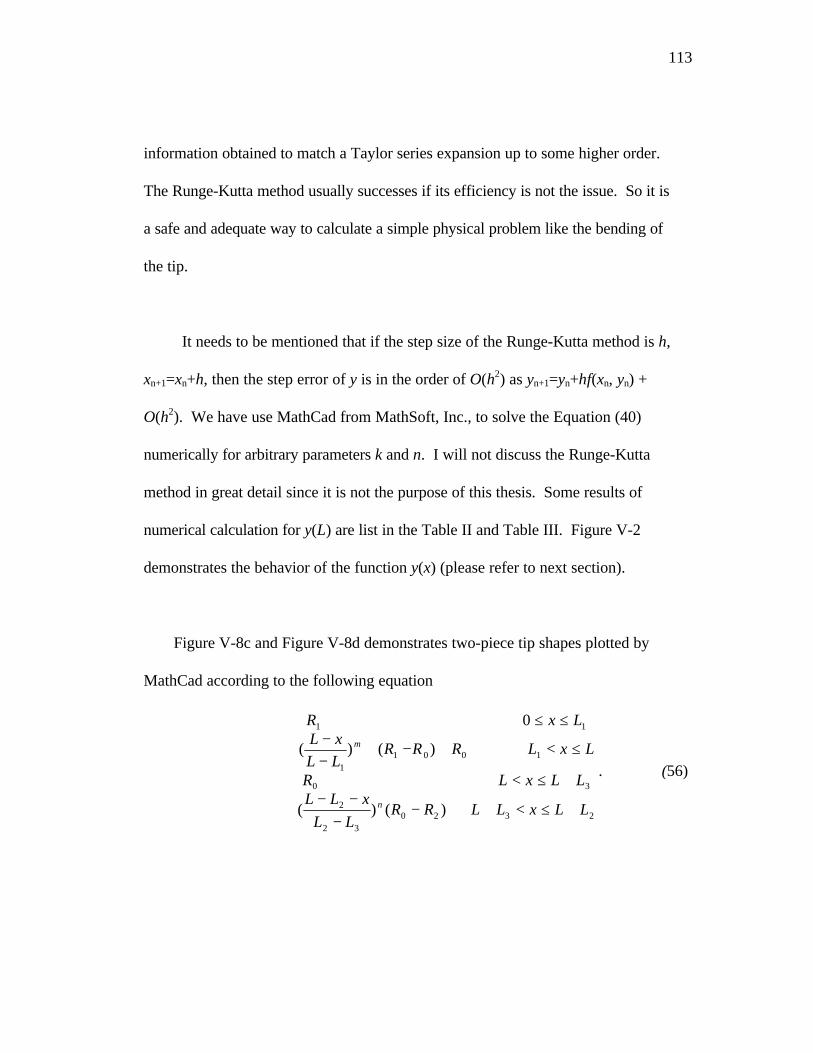
113

information obtained to match a Taylor series expansion up to some higher order.

The Runge-Kutta method usually successes if its efficiency is not the issue. So it is

a safe and adequate way to calculate a simple physical problem like the bending of

the tip.

It needs to be mentioned that if the step size of the Runge-Kutta method is h,

xn+1=xn+h, then the step error of y is in the order of O(h2) as yn+1=yn+hf(xn, yn) +

O(h2). We have use MathCad from MathSoft, Inc., to solve the Equation (40)

numerically for arbitrary parameters k and n. I will not discuss the Runge-Kutta

method in great detail since it is not the purpose of this thesis. Some results of

numerical calculation for y(L) are list in the Table II and Table III. Figure V-2

demonstrates the behavior of the function y(x) (please refer to next section).

Figure V-8c and Figure V-8d demonstrates two-piece tip shapes plotted by

MathCad according to the following equation

+≤<+−−

−−+≤<

≤<+−−−

≤≤

232032

2

30

10011

11

)()(

)()(

0

LLxLLRRLL

xLLLLxLR

LxLRRRLL

xLLxR

n

m

. (56)

114

For the definition of parameters, please refer to Figure V-6. The power law indices

are m and n. R0, R1, and R2 are the radii of the tip as shown in Figure V-6 and

Figure V-8. From the bending curve in Figure V-7b and Figure V-7c, we can see

that most of the bending is from the smaller head segment.

When we try to apply the above method to a practical lateral displacement,

we face some problems especially for quantitative measurement of the lateral force.

First, it is difficult to measure the shape of a tip head32. Second, the shape of the tip

keeps changing during the scanning, because in air-based SPM there are interactions

between tip and sample surface that cause wear to the tip’s head (even for tapping

mode scanning force imaging). The interaction will change tip’s shape. What is

more, tip usually does not have a cylindrical symmetric structure. Third, the forces

acting on the tip come from different sources, and some of them are not only

applied on the very head of the tip. Especially for the air based scanning probe

microscopes, the adsorbed surface layer distributes the force at a certain region of

the tip.

Although these things make the quantitative analysis of the tip’s bending to

infer forces difficult, we may still be able to provide some qualitative estimates.

Table 5-1 lists calculated value of lateral displacements y(L) (in 102nm unit) for a

115

force of 98 nano Newton(nN), using tips with different power law indices n and tip-

reduction parameters k. The bending is Y(L)=38 nm for a lateral force of nano

Newton, which is in the plausible region. Certainly, adjusting tip’s dimensional

parameters will yield different lateral displacement.

Figure V-3 shows a numerical calculation of the displacement for the power

law index n=2. We can see that the bending is 0.1 micron for the tip head of 4 mm.

In this case, the tip’s head may be physically worn off (or curled up) until the head

is big enough to resist the force. Usually, we would like to make a tip as sharp as

possible. Practically, we see that a sharp tip with a cone angle too small (a large

power law index n) can not resist the friction force, and will be worn off (or bent

into a spiral) until the head is big enough.

For the numerical calculation, we must answer two questions. The first one is

how the physical parameters effect the calculation results and the second is how the

mathematical parameters effect the results. For this particular case, the physical

parameters are tip’s length, power law index and tip radii, and the mathematical

parameter is the sampling number (step size) for the integral.

116

The tip, with a point head of power-law index n less than 0.75, will have finite

displacement. If n is larger than 0.75, we might still have finite displacement

because in the real world, the bending force is not applied on a very point of the tip

head. The bending force is distributed in a finite region at the tip’s head. From our

numerical calculation, we can see that if the index n is between 0 to 0.70, the

displacement does not change significantly with k and L (please refer to Figure V-

2). Only when n is close to or larger than 0.75 does the displacement change

significantly. For an upper limit approximation to the lateral force, n=0.74 is

therefore not a bad choice. Figure V-2 displays the curves with different power law

indexes. The dependence of the lateral displacement for given force on tip with

different length is shown in Figure V-3. The calculation is done with a fixed tip

head length and a fixed power law index as 0.75 but the tail length of the tip

changes from 10R0 to 40R0. It seems that most of the bending is generated by the

tip head.

The number of sampling points, i.e., the number of steps in the calculation,

also will cause errors. Figure V-5 shows the change for the different step sizes

given the same values for n, k, and tip length. We can see that the curve has an

upper limit. N=106 will be accurate enough for us here. The above calculations

show that for a lateral force comparable to the data (~40 nN) given by other

117

researchers98, we can obtain a reasonable bending of the tip which is comparable to

our experimental lateral displacement data (~100 nm).

E. DISCUSSION

In the foregoing, we simply draw out the consequences of a classical

continuum-elasticity model for the relationship between lateral force and lateral

displacement for cylindrically symmetric tips whose radius as a function of position

along their length with a simple power law relationship. By combining several such

tip-segments in series, a wide range of tip shapes can be modeled and the quantitative

relationship between lateral force and lateral displacement be predicted.

A preliminary look at the variable space defined by these models suggests that

significant lateral forces must exist in air-based scanning tunneling microscopy, in

order for the displacements we observe to be thereby accounted for. If we assume

that lateral forces are smaller than those inferred in contact-mode atomic force

situations, in fact, it seems that small protrusions near the end of our tip may be

required. For example, if we model a tip made from the standard Pt-Ir wire of

commercial tips, and place a 10 micron protrusion 1 micron in diameter at the end

(with suitable conical caps for transition at each end), then a lateral displacement of

0.3 microns requires a force of just under 100 nN. This observation supports earlier

118

reports of significant forces between tunneling tips and their substrates, although

quantitative measurements of these forces have not been reported in the literature.

These calculations also suggest strategies for the design of tips sensitive to

the much smaller scan-direction-related lateral forces between tip and specimen that

might be present in ultra high vacuum STM studies. Although none of this requires

special equipment for data acquisition, quantitation will remain a challenge since it is

difficult to know and keep track of tip shape during an experiment.

119

Table II

n\N 300 3000 30000 3000000 0.880 0.884 0.884 0.884

0.14 0.880 0.884 0.884 0.8840.24 0.881 0.885 0.885 0.8850.34 0.883 0.887 0.887 0.8870.44 0.885 0.889 0.890 0.8900.54 0.889 0.894 0.894 0.8950.64 0.896 0.904 0.907 0.9070.74 0.912 0.939 0.961 0.980

Table II. Lateral displacement Y(L) with the power law index n and the number of

sampling steps N. The first column is n and the first row is N. The data in the body

of the table are the value of Y(L) as in nm unit. Other parameters are R0=0.1 mm,

L=18R0=1.8 mm, R1=10-4 R0 mm. We can see that for a larger power law index n,

the step size N plays a more important role than small power law index n, especially

for n near 0.75. The table also shows that the value of Y(L)/N approaches to finite

as N goes to ∞.

120

Table III.

m\N 1000 10000 50000 100000 500000 100000040 43.211 55.578 63.381 66.464 72.663 74.75730 11.055 13.755 15.464 16.14420 1.437 1.541 1.607 1.63410 0.151 0.152 0.152 0.152

Table III. The lateral displacement Y (nm) of different step number N and the

length of the tip as the ratio of m=L/R0. Here L is the total length of the tip and R0

is the radius of the tip. The length of tip’s head is 3R0. We can see that the bending

curve has an up boundary. So, N=106 will be good enough for the numerical

calculation.

121

R

dx

dθ

drr

Center Line

F

-F

T

-T

L=dx

dxdr

Center

Beam

Beam Segment

Figure V-1. Figure V-1a shows a bending segment of a beam. The central line of

the segment keeps unchanged. A segment, which is away from the central line, will

be stretched or contracted and then produces stress to resist the bending. Figure V-

1b is the zoom out view of Figure V-1a. The bending of the segment is caused by a

force couple.

5-1a

5-1b

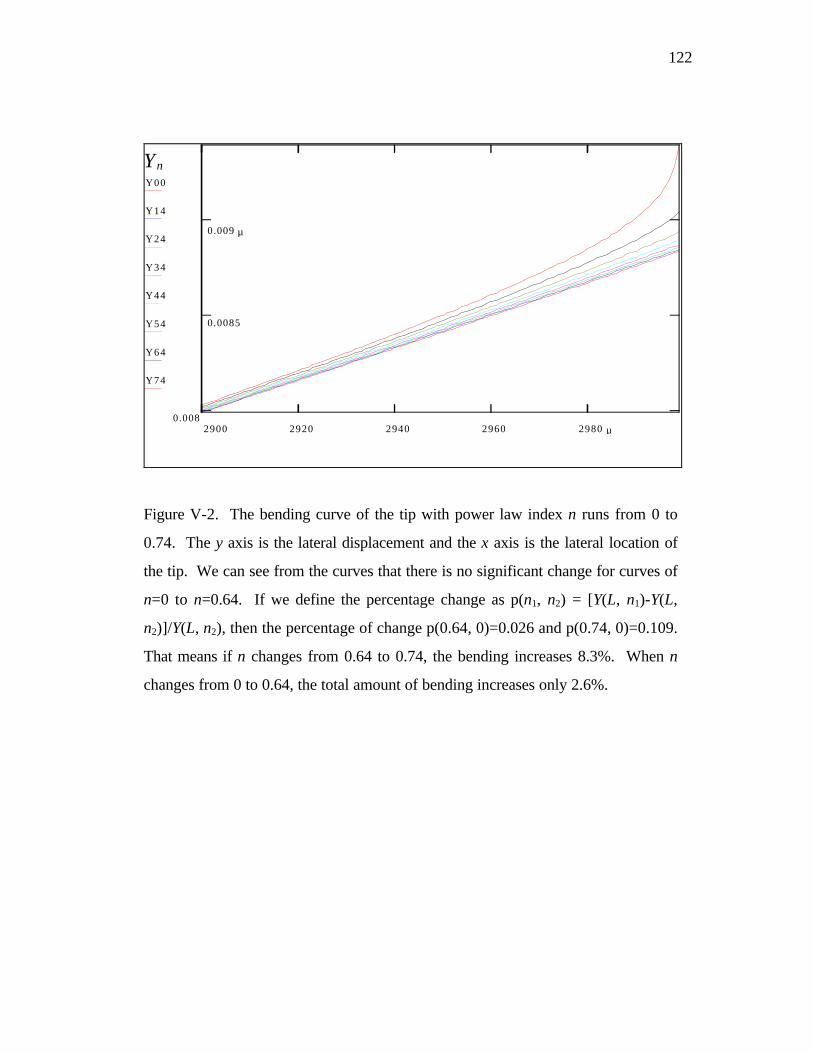
122

2900 2920 2940 2960 2980 µ0.008

0.0085

0.009 µ

Y00

Y14

Y24

Y34

Y44

Y54

Y64

Y74

Yn

Figure V-2. The bending curve of the tip with power law index n runs from 0 to

0.74. The y axis is the lateral displacement and the x axis is the lateral location of

the tip. We can see from the curves that there is no significant change for curves of

n=0 to n=0.64. If we define the percentage change as p(n1, n2) = [Y(L, n1)-Y(L,

n2)]/Y(L, n2), then the percentage of change p(0.64, 0)=0.026 and p(0.74, 0)=0.109.

That means if n changes from 0.64 to 0.74, the bending increases 8.3%. When n

changes from 0 to 0.64, the total amount of bending increases only 2.6%.

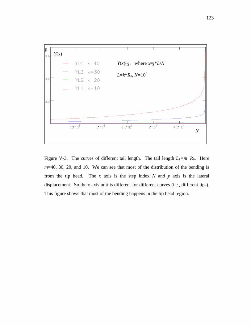
123

µ

Y(x)~j, where x=j*L/N

L=k*R0, N=105

N

Y(x)

Figure V-3. The curves of different tail length. The tail length L1=m×R0. Here

m=40, 30, 20, and 10. We can see that most of the distribution of the bending is

from the tip head. The x axis is the step index N and y axis is the lateral

displacement. So the x axis unit is different for different curves (i.e., different tips).

This figure shows that most of the bending happens in the tip head region.

124

0 1 2 3 4 5 6 J

0.009

0.0092

0.0094

0.0096 Y(L)~n[j]

nm

Figure V-4. The lateral displacement Y(L) vs. power law index n. For the

convenience of the drawing, the x axis represents power law index n as: x0 =0, x1

=0.14, x2 =0.24, x3=0.34, x4=0.44, x5=0.54, x6=0.64, and x7 =0.74. This figure

shows the increasing speed of the bending vs. the power index n.

125

Step N

Y(L)*102(nm)

Y(L) ~ Step number N

Figure V-5. The curve of displacement Y(L) (y-axis) as a function of sampling

number N (step number N, x axis). This curve shows that the displacement has an

up limit for the sampling number. That means the curve is convergent under the

sampling number N. The parameters of the tip are: length L=40R0, tip head = 3R0,

and n= 0.74. We can see that the curve approaches to a limit around 0.75 nm.

This figure also shows that the calculation using MathCad is convergent and

N=5×105 is enough for the discussion.

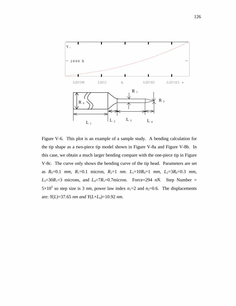
126

L 1

R 0

L 2 L 3 L 4

R 1

R 2

t j

Y j

2 0 0 0 Å

µ

Figure V-6. This plot is an example of a sample study. A bending calculation for

the tip shape as a two-piece tip model shown in Figure V-8a and Figure V-8b. In

this case, we obtain a much larger bending compare with the one-piece tip in Figure

V-8c. The curve only shows the bending curve of the tip head. Parameters are set

as R0=0.1 mm, R1=0.1 micron, R2=1 nm. L1=10R0=1 mm, L2=3R0=0.3 mm,

L3=30R1=3 microns, and L4=7R1=0.7micron. Force=294 nN. Step Number =

5×105 so step size is 3 nm, power law index n1=2 and n2=0.6. The displacements

are: Y(L)=37.65 nm and Y(L+L4)=10.92 nm.

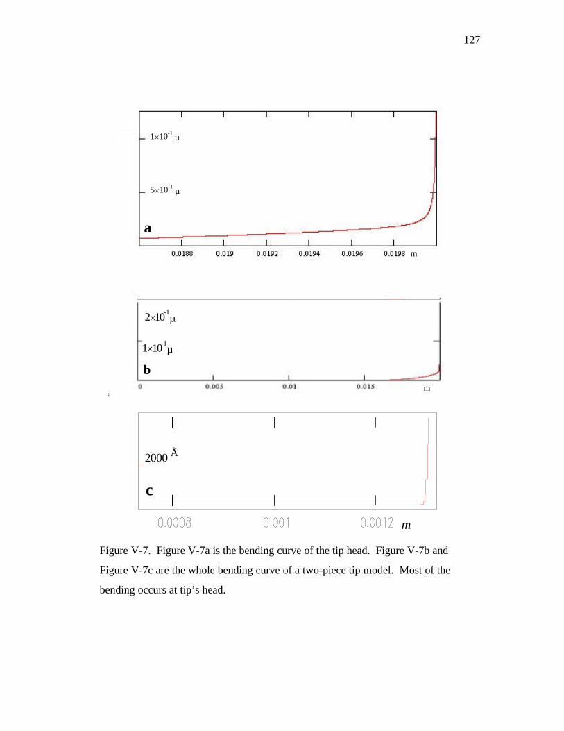
127

1×10-1 µ

5×10-1 µ

m

a

2×10-1µ

1×10-1µ

m

b

2000 Å

m

c

Figure V-7. Figure V-7a is the bending curve of the tip head. Figure V-7b and

Figure V-7c are the whole bending curve of a two-piece tip model. Most of the

bending occurs at tip’s head.

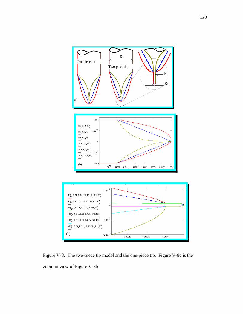
128

R1

Ro

R2

Two-piece tipOne-piece tip

(a)

(b)

(c)

Figure V-8. The two-piece tip model and the one-piece tip. Figure V-8c is the

zoom in view of Figure V-8b

129

VI. SUMMARY OF RESULTS

In this thesis, we developed a method to infer the vector lateral displacement

between two images of essentially the same objects by using correlation-based

displacement mapping (including rotational displacement if desired). Although

similar algorithms have been used in the past for topographic studies, we are

unaware of an implementation general enough for scanned probe microscope

applications. The physical meaning of the lateral displacement map depends on the

process that creates the “differing” image pairs. The resolution of the resulting

image maps relies on the texture resolution of the image and generally is lower than

the original images. This lateral mapping method should work for n-dimensional

image sets as well as for 2-dimensional image pairs. The effectiveness of our

algorithm for a more traditional application, namely quantifying topography from

image stereo-pairs, was demonstrated with an example.

The mapping algorithm was then used to quantify vector lateral

displacements, for the first time, between scanning tunneling microscope image

pairs with different scan directions such as left-right (X - (-X)) or left-up (X-Y).

This allowed us to store the x and y components as separate image maps.

Acquiring the images required no special hardware and can be done with any STM

130

capable of recording scan and rescan images. Such lateral displacement maps of

STM hologram image pairs show that the spatial frequency of lateral displacement

across the corrugated hologram structure is twice that of the spatial frequency of

the topographic corrugation in the scan direction.

A simple, classical friction model of lateral force on the tip explains the

spatial frequency, the phase, and the direction of the observed displacements, if we

assume only that the friction force is constant in magnitude. This assumption

seems plausible in air-based scanning tunneling microscopy if friction is

proportional to the normal force, since a constant tunneling current will likely

require that the normal force between tip and specimen be held constant as well.

The model therefore indicates that the measured lateral displacements come from

friction between the tip and the sample. The model also suggests that

displacements will be simply proportional to coefficient of friction even in the

presence of significant topography. Lateral force microscope image contrast is

dominated by coefficient of friction differences only when topography plays a

small role. In either case, the topographic effects (if they follow the classical

model as in the work here) are possible to model and remove from the maps.

131

The work reported here also shows that lateral force microscope images,

taken using a constant force rather than a constant current feedback loop, show a

doubled spatial frequency on holograms as well. Unlike the STM lateral

displacement maps, the lateral force double spatial frequency profiles are

asymmetric. Beside the double spatial frequency feature, we find a set of

secondary-minima in the lateral force profiles. Those secondary minima are

located at high slope areas on each side of the hologram corrugation being

traversed by the tip. We explain these secondary minima by a model in which

twists of the cantilever are due to a combination of the normal and frictional force.

Uphill traveling yielded a larger twisting of the cantilever than did downhill

traveling. Thus according to this model, LFM measures a combination of friction

coefficient µ and topographic tangent angle α.

Lastly, we calculated the relationship between tip shape, bending, and the

size of lateral forces involved. Thus, these first measurements of tip lateral

displacement in the scanning tunneling microscope allow us to make the first

estimates of tip lateral force as well. Although we do not have shape data on the

specific tips used to take data in Chapter 2, the calculations and our examination

of other tips suggest that the observed tip bending will likely require forces on the

order of 100 nN. Thus, this result follows the early TEM work of specimen lattice

132

bending by Lo et al.43, and is as independent confirmation of the significant

interaction forces between tip and specimen in STM at non-UHV pressures.

Interestingly, researchers involved in scanning tip microscopy often struggle

to make and keep their tips as sharp as possible with a small cone angle as well.

How sharp is practicable? Our calculations show that if the tip is too sharp, i.e.,

with a very small cone angle, the tip probably will be altered at first contact until the

tip head is worn off or bent sufficiently to sustain the lateral force. Numerical

calculation shows that tip shapes with power law indices less then 0.75 are

practicable, at least in theory. The results also suggest that STM lateral

displacement studies at low pressure should now allow exploration of scan-direction

dependent lateral forces in ultra-high-vacuum STM, if they exist, as well as the

onset of friction forces on the nanoscale as atmospheric pressures are allowed to

increase.

133

APPENDIX

A. The Constants C and D in Equation (5) and Equation (6)

We can calculate the constants C and D if the SEM image system obeys theoptical equation

fss111

=+'

. (A-1)

From Figure II-15, we have

fsHs111

1

=+− '

, (A-2)

'

'

1

1

s

xHs

x=

−. (A-3)

If α<<1, H/(s-f) <<1 and x/(s-f) <<1, we have

fsxHs111

2

=++− 'α

, (A-4)

'

'

2

2

s

x

xHsxH

=+−+

αα

. (A-4)

Thus, the x displacement dx is

HCHfs

fxxdx ⋅=

−≈−=

α''12 . (A-5)

Similarly, from Figure II-16, we have

fsHs111

1

=+− '

, (A-6)

'

'

1

1

s

y

Hsy

=−

, (A-7)

fsxHs111

2

=++− 'α

, (A-8)

'

'

2

2

s

yxHs

y=

+− α. (A-9)

And dy as

134

0212 ≈⋅=

−≈−= xyDxy

fsf

yydy)(

'' α. (A-10)

135

B. The measurement of Young's modulus of the Pt/Pr wire:

We use a piece of Pt/Pr wire of length L=8.5 cm and radius R=0.001 cm. One

end is fixed at wall horizontally and another end is hanged with a piece of paper.

The weight of this piece of paper is W=0.2106g. The total bending is B=2.1 cm.

According the calculation made by Chapter Five, we have Pt/Pr wire’s Young’s

modulus as E=0.7×1010 kg m-2

136

C. The Semper6 Code of Lateral Displacement Mapping

LIST C-1

Generate distorted image (add the distortion to the images).

calculate x + fg2 to im1

calculate y to im2

stack im1, im2 to im3

reclass im3 plist

extract fg1 with im3 to fg4

calculate x to im1

calculate y+fg3 to im2

stack im1, im2 to im3

reclass im3 plist

extract fg1 with im3 to fg5

LIST C-2

Remove distortion from the images

calculate x - fg6 to im1

calculate y to im2

stack im1, im2 to im3

reclass im3 plist

extract fg4 with im3 to fg8

calculate x to im1

copy y - fg7 to im2

137

stack im1, im2 to im3

reclass im3 plist

extract fg5 with im3 to fg9

LIST C-3

Correlation mapping program.

!!!!!!!!!!!!!!!!!!!!!!!!!!!!!!!!!!!!!!!!!!!!!!!!!!!!

! /home/newton/staff/semper/dis.run

! displacement mapping program

! version 1.0 UM-St. Louis Department of Physics and

! Astronomy and Center for Molecular Electrons.

! Chang Shen 1992, Original: Phil Fraundorf

!!!!!!!!!!!!!!!!!!!!!!!!!!!!!!!!!!!!!!!!!!!!!!!!!!!!

type 'displacement mapping'

type 'normal version, version 1.0 UMSL sc (ori pf)'

p00=4:1

ask 'name of image A (last dig # of first image )(rtn=4:1) '

p98

unless set(p98) p98=4:1

138

if p98 ~= p00 jump T99

ask 'name of image B (rtn=4:2) ' p99

unless set(p99) p99=4:2

T99:

ask 'number of series start (rtn=4:3) ' p03

unless set(p03) p03=4:3

ask 'Step of series images (rtn=3) ' sp1

unless set(sp1) sp1=3

ask 'No. of series images (rtn=1) ' sp2

unless set(sp1) sp2=1

sp0=0

p04=p03+1

p05=p03+2

p06=p03+3

p07=p03+4

p08=p03+5

p09=p03+6

p10=p03+7

139

p11=p03+8

p14=p03+11

p15=p03+12

p16=p03+13

p17=p03+14

p18=p03+15

p19=p03+16

p20=p03+17

p21=p03+18

p22=p03+19

p01=p03-2

p02=p01+1

ask 'step size in pixels (rtn=1) ' a81

unless set(a81) a81=1

ask 'max. size of block in x 2^i (rtn=2) ' itx

unless set(itx) itx=2

!ask 'max. size of block in y 2^i (rtn=2) ' ity

!unless set(ity) ity=2

140

! Main loop

L77:

if p98=p00 jump L99

m99=100+p98

m88=200+p98

ass name 'sc/dsk/df/df1/',m99

cop n:1 to p01

deas dev n

ass name 'sc/dsk/df/df1/',m88

cop n:1 to p02

deas dev n

L99:

sur p02 ful nover

origin p02 reset

sur p01 ful nover

origin p01 reset

141

pcb p01

x=0; y=0

npx=ncols; npy=nrows

cop p01 to p03

mask p03 to p04 out rad npx/6 pos 0,0

npx=ncols; npy=nrows

cop p01 to p03

mask p03 to p04 out rad npx/6 pos 0,0 width 1

xex=npx/2-npx/16; yex=npy/2-npy/16

xold=0; yold=0

create p15 size npx,npy value 0 fp

xcf p01 with p02 to p15

yy0=y

type 'creating topographic map...'

create p03 size npx,npy value 0 fp

create p05 size npx,npy value 0 fp

142

create p06 size npx,npy value 0 byte

create p04 size npx,npy value 0 fp

create p07 size npx,npy value 0 fp

title p03 text 'x-displacement'

title p05 text 'correlation coefficient'

title p06 text 'optimal correlation coefficient'

title p04 text 'y-displacement'

title p07 text 'peek pixel value'

!get average displacement first

xcf p01 with p02 to p07

survey p07 ful noverify

trap=77 peaks p07 to p08 radius thresh max-sd

select p07

if rc=77 p 0,0,0=ax0

if rc=77 p 0,1,0=ay0

! xp0,yp0 are average displacement

xp0=p(0,0,0)

143

yp0=p(0,0,1)

ax0=xpk

ay0=ypk

!-- begin main loop

i0=-xex

a02=4

L01:

j0=-yex

type 'image=',p98,' (column,row)=(',i0,';',j0,')'

L02:

! Now we are at i0,j0

x01=i0; y01=j0;

w2x=0; ww0=0; tmx=-1; xmx=0;

wlst=0; dx=0; imx=0; tmo=0; ich=1; xold=0; i=4

yold=0; dy=0

L03:

144

if tmx=tmo | i>6 ich=-1

if tmx=tmo | i>6 dx=dx+xold

if tmx=tmo | i>6 dy=dy+yold

if i<7 & tmx=tmo i=i-1

if i>6 i=i-2

xold=x

yold=y

tmo=tmx

a01=2^i

m01=256/a01

a02=(a01/8)+1

!Cut a square from p01 at (x01,y01) to p09

extr p01 to p09 size a01 pos x01,y01

!Cut a square at (xx01,yy01) from p02 to p10

xx01=x01+dx;yy01=y01+dy

extr p02 to p10 size a01 pos xx01,yy01

!X corr. function of p09 and p10

xcf p09 with p10 to p07

!Get the displacement value in fp

145

survey p07 full noverify

trap=77 peaks p07 to p08 radius 1 thresh max-sd

select p07

if rc=77 p 0,0,0=ax0

if rc=77 p 0,1,0=ay0

!temp. displacement xpk,ypk

xpk=p(0,0,0)

ypk=p(0,0,1)

! For later use of average displacement ax0,ay0

ax0=xpk

ay0=ypk

if t<tmx jump TS1

xmx=xpk+dx

ymx=ypk+dy

imx=i

tmx=t

TS1:

146

!square became smaller, use new displacement

if ich=-1 dx=dx+x

if ich=-1 dy=dy+y

if tmx>tmo i=i+ich

!The best result for this location (x01,y01)

if i>itx & (ich>0 | tmx>tmo) jump L03

select p03

p i0,j0,0=xmx

select p08

p i0,j0,0=tmx

select p09

p i0,j0,0=imx

select p10

p i0,j0,0=ymx

j0=j0+a81

! next column

if j0<yex jump L02

i0=i0+a81

147

!next row

if i0<xex jump L01

save p03 name 'cs/dx',p98

save p04 name 'cs/dy',p98

save p05 name 'cs/mx',p98

save p06 name 'cs/mc',p98

type 'Done of displace.run !!!'

end

148

BIBLIOGRAPHY

1 G. Binnig, and H. Rohrer, Scanning tunneling microscopy, Helvetica Physica Acta55, 726 (1982).

2 G. Binnig, and H. Rohrer, Scanning tunneling microscopy, IBM J. Res. Develop.A30, 355 (1986).

3 G. Binnig, and H. Rohrer, Rev. Mod. Phys. 59, 615 (1987); P. K. Hansma and J.Tersoff, J. Appl. Phys. 61 R1 (1987).

4 T E. Feuchtwang, and P H. Cutler, Tunneling and scanning tunnel microscopy: Acritical review, Physica Scripta 35(2) Feb, 132 (1987).

5 V S. Edel'man, Scanning tunneling microscopy (review), Instruments &Experimental Techniques 32(5) Mar, 993 (1990).

6 G. Binnig, C. F. Quate, and Ch. Gerber, Scanning force microscopy, Phys. Rev.Lett. B56, 930 (1986).

7 G. Binnig, et al., Atomic resolution with atomic force microscope, Europhys.Lett. 3, 1281 (1987).

8 H. Salemink, and O. Albrektsen, Applications of scanning tunneling microscopyto the characterization of semiconductor technologies and devices,Microelectronic Engineering 15 (1-4) Oct, 101 (1991).

9 W. Mirande, H. Geuther, and H. Jacobsen, Accuracy in critical dimensionmeasurements on integrated circuits and photomasks, MicroelectronicEngineering 30 (1-4) Jan, 587 (1996).

10 M. P. Green, Electrochemical applications of scanning probe microscopy,Materials Technology 9 (5-6) May-June, 100 (1994).

149

11 J. Mayer, et al., Characterization of thermally oxidized carbon fiber surfaces byESCA, wetting techniques and scanning probe microscopy, and the interactionwith polyethylmethacrylate, Development Of A Biocompatible CompositeMaterial Composites 25 (7), 763 Aug., (1994).

12 B. L. Blackford, M. H. Jericho, and P J. Mulhern, Review of scanning tunnelingmicroscope and atomic force microscope imaging of large biological structures:problems and prospects, Scanning Microscopy 5 (4), 907 Dec., (1991).

13 C. R. Clemmer, and T. P. Beebe Jr., Review of graphite and gold surface studiesfor use as substrates in biological scanning tunneling microscopy studies,Scanning Microscopy 6 (2), 319 Jun., (1992).

14 R. J. Wilson, K. E. Johnson, D. D. Chambliss, and B. Melior, Scanning tunnelingmicroscopy of biological molecules on Pt(111): from 100 to 5 multiplied by 106,Da Langmuir 9 (12), 3478 Dec., (1993).

15 V. T. Moy, et al., Probing the forces between complementary strands of DNAwith the atomic force microscope, Proceedings of SPIE-The International Societyfor Optical Engineering 2384, (1995), (Society of Photo-Optical InstrumentationEngineers, Bellingham, WA, USA.) pp. 2-12.

16 S. M. Lindsay, et al., Scanning tunneling microscopy and atomic forcemicroscopy studies of biomaterials at a liquid-solid Interface, J. Vac. Sci.Technol. A 11(4), 808 (1993).

17 A. A. Gewirth, and B. K. Niece, Electrochemical applications of in situ scanningproblem microscopy, Chemical Reviews, 1129 June, (1997).

18 T. Koshikawa, et al., Surface structure of Cu/Si(111) at high temperature,Surface Science 331-333 A July, 506 (1995).

19 A. W. Stephenson, T. M H. Wong, and M. E. Welland, Ambient and hightemperature STM investigations of the growth of titanium silicide on siliconsubstrates, Evolution of Thin Film and Surface Structure and MorphologyMaterials Research Society Symposium Proceedings 355, (1995) (MaterialsResearch Society, Pittsburgh, PA, USA.) pp. 287-292.

150

20 J. A N. Zasadzinski, et al., Scanning tunneling microscopy of freeze-fracturereplicas of biomembranes, Science 239 (4843), 1013 Feb. 16, (1988).

21 T. G. Lenihan, A P. Malshe, W. D. Brown, and L. W. Schaper, Artifacts inSPM measurements of thin films and coatings, Thin Solid Films, 270 (1-2), 356Dec., (1995).

22 D. J. Keller, et al., Envelope reconstruction of probe microscope images, SurfaceScience 294, 409 (1993).

23 S. S. Sheiko, M. Moller, E M C M. Reuvekamp, and H W. Zandbergen,Evaluation of the probing profile of scanning force microscopy tips,Ultramicroscopy 53 (4), 371 Apr., (1994).

24 H. J. Butt, Electrostatic interaction in atomic force microscopy, Biophys. J.(USA) 60(4), 777 (1991); X.Y. Lin, F. Creuzet, and H. Arribart, Atomic forcemicroscopy for local characterization of surface acid-base properties, J. Phys.Chem. 97, 7272 (1993); C.D. Frisbie, et al., Functional group imaging bychemical force microscopy, Science 265, 2071 Sept. 30, (1994).

25 Y. Martin, and H. K. Wickramasinghe, Appl. Phys. Lett. 50, 1455 (1987).

26 R. Wiesendanger, et al., Recent advances in scanning tunneling microscopyinvolving magnetic probes and samples, Applied Physics A-Solids & Surfaces 53(5), 349 Nov., (1991).

27 U. Hartmann, Scanning probe microscopy on superconductors: achievementsand challenges, Applied Physics A-Solids & Surfaces 59 (1), 41 July, (1994).

28 D. W. Pohl, Some thoughts about scanning probe microscopy, micromechanics,and storage, IBM J. of Res. & Develop. 39 (6), 701 Nov. (1995).

29 M. J. Allen, et al., Tip-radius-induced artifacts in AFM images of protamine-complexed DNA fibers, Ultramicroscopy 42-44, 1095 (1992).

30 S. Vieira, The behavior and calibration of some piezoelectric ceramics used inthe STM, IBM J. Res. Develop. 30 (5), 553 (1986)

151

31J. E. Griffith, and D. A. Grigg, Dimensional Metrology with Scanning ProbeMicroscopes, J. Appl. Phys. 74(9) (1993) page R83.

32 P. Fraundorf, and J. Tentschert, The instrument response function in air-basedscanning tunneling microscopy, Ultramicroscopy 37, 125 (1991).

33 J. S. Villarrubia, Morphological estimation of tip geometry for scanned probemicroscopy, Surface Science 321 (3), 287 Dec., 20 (1994).

34 Masato Aketagawa, and Koji Takada, Correction of distorted STM image byusing a regular crystalline lattice and 2D FFT, Nanotechnology 6 (4), 105 Oct.,(1995).

35 J. Krim, Friction at the atomic scale, Scientific American, 74 Oct., (1996).

36 E. Meyer, et al., Atomic Force Microscopy For The Study Of Tribology andAdhension, Thin Solid Films (Switzerland), (1989) (San Diego, CA, USA.)

37 M. Binggeli, and C. M. Mate, Influence of capillary condensation of water onnanotribology studied by force microscopy, Appl. Phys. Lett. (USA) 65(4), 415(1994).

38 I. L. Singer, et al., Fundamentals of Friction: Macroscopic and microscopicprocesses, Dordrecht, (1992).

39 M. G. Heaton, C. B. Prater, and K. J. Kjoller, Lateral and chemical forcemicroscopy mapping surface friction and adhension, Instruments notes ofDigital Instruments, Inc.

40 C. B. Prater, P. G. Maivald, K. J. Kjoller, and M. G. Heaton, Probing nano-scaleforce with the atomic force microscope, Instruments Notes of Digital Instruments,Inc.

41 A. Peled, et al., Characterization of photodeposited selenium planar structuresby scanning force microscopy, J. of Appl. Phys. 77 (12), 6208 Jun, 15 (1995).

152

42 S D. Campbell, et al., Spectral and structural features of porous silicon preparedby chemical and electrochemical etching processes, J. of Vac. Sci. & TechnologyB 13 (3), 1184 May-Jun., (1995).

43 R. Kaneko, Microtribology today and tomorrow, Wear. 168 (1-2), 1 Sept. 1,(1993).

44 N. K. Myshkin, S A. Chizhik, and V. V. Gorbunov, Nanoscale topography andtribological problems, Tribology International. 28 (1), 39 (1995).

45 J. C. H. Spence, et al., J. Vac. Sci. Technol., A7, 2745 (1989).

46 J. A. Stroscio, R. M. Feenstra, and A. P. Fein, Phys. Rev. Lett. 57, 2579 (1986).

47 G. Binnig, H. Rohrer, Ch. Gerber, and E. Weibel, Appl. Phys. Lett. 40, 178(1982).

48 J. H. Coombs, and J. B. Pethica, Properties of vacuum tunneling currents:Anomalous barrier heights, IBM J. Res. Develop. 30, 455 (1986).

49 J. M. Soler, A. M. Baro, N. Garcia, and H. Rohrer, Interatomic forces inscanning tunneling microscopy: Giant corrugations of the graphite surface,Phys. Rev. Lett. 57, 444 (1986).

50 H. J. Mamin, et al., Phys. Rev. B 34, 9015 (1986).

51 J. Tersoff, and N. D. Lang, Phys. Rev. Lett. 65, 1132 (1990).

52 W. Hanrieder, R. Mock, and H. Meixner, The whip motion of ultra-thintunneling tips, Ultramicroscopy 42-44, 169 (1992).

53 Dror Sarid, Scanning force microscopy with applications to electric, magnetic,and atomic forces, Oxford University Press (1991) pp. 197.

54 G. Mayer, and N. M. Amer, Appl. Phys. Lett. 53 1044 (1988).

55 D. Rugar, and P. Hansma, Phys Today 43(10), 23 (1990).

153

56 Y. Martin, C. C. Williams, and H. K. Wickramasinghe, Atomic force microscope-force mapping and profiling on a sub 100 Å scale, J. Appl. Phys. 61, 4723(1987).

57 G. M. McClelland, R. Erlandsson, and S. Chiang, Review of progress inquantitative nondestructive evaluation, Vol. 6B, D. O. Thompson and D. E.Chimenti. eds., (Plenum, New York, 1987) pp. 307.

58 H. K. Wickramasinghe, Methods of Experimental Physics, Vol. 27 ScanningTunneling Microscopy, Academic Press, Inc. (1993) pp. 88.

59 Alexander L. Shluger, Andrew L. Rohl, R M. Wilson, and R T. Williams,Atomistic modeling of imaging of ionic surfaces with a scanning forcemicroscope, J. of Vacu. Sci. & Technol. B 13 (3), 1155 May-Jun. (1995).

60 W. H. Press, B. P. Flannery, S. A. Teukolsky, and W. T. Vetterling, NumericalRecipes, Cambridge University Press (1988) pp. 400-449

61 V. Lipovac, Zero-crossing-based linear prediction for speech recognition,Electronics Lett. 25 (2), 90 Jan 19 (1989).

62 David Mansour, Biing Hwang Juang, Short-time modified coherencerepresentation and its application for noisy speech recognition,

Proceedings - ICASSP, IEEE International Conference on Acoustics, Speech andSignal Processing 1-5 (Piscataway, NJ, USA, 1988) pp. 525-528 (Available fromIEEE Service Cent, Cat. Publ by IEEE, New York, NY, USA. n 88 CH2561-9).

63 V. V. Apanasovich, and E G. Novikov, Identification of lifetime characteristicsin fluorescence experiments, Proceedings of SPIE - The International Society forOptical Engineering. v 2388 (Society of Photo-Optical Instrumentation Engineers,Bellingham, WA, USA, 1995) pp. 378-384

64 Massimiliano Martone, Blind deconvolution in spread spectrum communicationsover non minimum phase channels, IEEE MILCOM. 2 (IEEE, Piscataway, NJ,USA, 1994) pp. 463-467 (94CH3400-9)

154

65 Douglas A. Ross, and Nicholas Dimas, Particle sizing by dynamic lightscattering: Noise and distortion in correlation data, Particle & Particle SystemsCharacterization 10 (2), 62 Apr. (1993).

66 Nicholas Lange, Variability and covariability in magnetic resonance functionalneuroimaging, Proceedings of SPIE - the International Society for OpticalEngineering, 2299, (1994) pp. 150-160

67 S. Pfleiderer, D G A. Ball, and R C. Bailey, AUTO: A computer program for thedetermination of the two-dimensional autocorrelation function of digital images,Computers & Geosciences 19 (6), 825 Jul., (1993).

68 Ying-Lin Yu, and Li-Hong Ma, Image reconstruction by an extendautocorrelation method, China 1991 International Conference on Circuits andSystems; China 91 Int Conf Circuit Syst. Publ by IEEE, IEEE Service Center,Piscataway, NJ, USA (IEEE cat n 91TH0387-1), pp. 582-583

69 Noel Bonnet, On the use of correlation functions for improving the imagesignal-to-noise ratio, Optik 80 (3), 103 Oct., (1988).

70 Jean-Claude Rajaonah, Bruno Dousse, and Jean-Jacques Meister, Compensationof the bias caused by the wall filter on the mean Doppler frequency, IEEETransactions on Ultrasonics Ferroelectrics & Frequency Control 41 (6), 812Nov., (1994).

71 H. Lee, and H. Oshima, New crack-imaging procedure using spatialautocorrelation function, Journal of Transportation Engineering 120 (2), 206Mar.-Apr. (1994).

72 Pietro A. Brivio, Ilaria Doria, and Eugenio Zilioli, Aspects of spatialautocorrelation of Landsat TM data for the inventory of waste-disposal sites inrural environments, Photogrammetric Engineering & Remote Sensing, 59 (9),1377 Sept. (1993).

73 C. D. Knittle, and N. Magotra, Image enhancement using the adaptivecorrelation enhancer, IEEE Transactions on Circuits & Systems II-Analog &Digital Signal Processing 39 (12), 862 Dec., (1992).

155

74 Bishnu S. Atal, Richard V. Cox, and Peter Kroon, Spectral quantization andinterpolation for CELP coders, Proceedings - ICASSP, IEEE InternationalConference on Acoustics, Speech and Signal Processing Vol. 1(of 4). (Availablefrom IEEE Service Cent. cat. Publ by IEEE, IEEE Service Center, Piscataway,NJ, USA. n 89CH2673-2), Piscataway, NJ, USA pp. 69-72.

75 K. W. Fleischer, et al., Cellular texture generation, Proceedings of the ACMSIGGRAPH Conference on Computer Graphics, (ACM, New York, NY, USA1995) pp. 239-248.

76 J. R. Logie, and J W. Patterson, Inverse displacement mapping in the generalcase, Computer Graphics Forum 14 (5), 261 Dec., (1995).

77 V. Burdin, C. Roux, C. Lefevre, and E. Stindel, Modeling and analysis of 3-Delongated shapes with applications to long bone morphometry, IEEETransactions on Medical Imaging, 15 (1), 79 Feb., (1996).

78 Dennis A. et al., Object tracking through adaptive correlation, Proceedings ofSPIE - The International Society for Optical Engineering 1959, (1993) pp. 314-321 (Publ by Society of Photo-Optical Instrumentation Engineers, Bellingham,WA, USA).

79G. Bonmassar, and E. L. Schwartz, Geometric invariance in space-variant visionsystems: The exponential chirp transform, Proceedings - International Conferenceon Pattern Recognition 3, (1994) pp. 204-207 (IEEE, Piscataway, NJ, USA,94CH3440-5).

80 S. M. Seitz, and C. R. Dyer, View Morphing, (Preprint for ACM ComputerGraphic Proceedings, Annual Conference Series, 1996)

81 E. Nezry, M. Leysen, and G. De Grandi, Speckle and scene spatial statisticalestimators for SAR image filtering and texture analysis: some applications toagriculture, forestry, and point targets detection, Proceedings of SPIE-TheInternational Society for Optical Engineering 2584, (1995) pp. 110-120 (Societyof Photo-Optical Instrumentation Engineers, Bellingham, WA, USA).

82 M. Radmacher, et al, Science, Vol. 257, 1901 Sept., (1992).

156

83 Takashi Okamoto, Yuuki Egawa, and Toshimitsu Asakura, Liquid crystaltelevision applied to a speckle correlation method Real time measurement of theobject displacement. Optics Communications, 88 (1), 17 Mar. 1, (1992).

84Jae Kyu Lee, and Won Chul Jhee, Two-stage neural network approach for ARMAmodel identification with ESACF, Decision Support Systems 11 (5), 461 Jun.,(1994).

85 Wolfgang Krueger, Intensity fluctuations and natural texturing ComputerGraphics (ACM), 22 (4), 213 Aug. (1988).

86 Dennis A. Montera, et al., Object tracking through adaptive correlation,Proceedings of SPIE - The International Society for Optical Engineering 1959,314 (1993). (Publ by Society of Photo-Optical Instrumentation Engineers,Bellingham, WA, USA ).

87 Lisa G. Brown, and H. Shvaytser, Surface orientation from projectiveforeshortening of isotropic texture autocorrelation, Proc CVPR 88 Comput Soc.Conf. on Comput Vision and Pattern Recognit, (1988) pp.510-514 (Availablefrom IEEE Service Cent, cat. Publ by IEEE, New York, NY, USA 88CH2605-4,Piscataway, NJ, USA).

88 R. Srinivasan, Autocorrelation For Structure Identification In Satellite Images,Publ by IEEE, New York, NY, USA. n 87CH2423-2, Piscataway, NJ, USA pp.86-90.

89 William J III Dunn, et al., Preprocessing, variable selection, and classificationrules in the application of SIMCA pattern recognition to mass spectral data,Environmental Science & Technology 23 (12), 1499 Dec. (1989).

90 R. Dong, S. Chu, and J. Katz, Quantitative visualization of the flow within thevolute of a centrifugal pump, Part A: technique, Journal of Fluids Engineering-Transactions of the ASME 114 (3), 390 Sept. (1992).

157

91H. Singh, and A. Mahalanobis, Correlation filters for texture recognition andapplications to terrain-delimitation in wide-area surveillance. Proceedings -ICASSP, IEEE International Conference on Acoustics, Speech and SignalProcessing 5, (1994) pp. V-153-156 (IEEE, Piscataway, NJ, USA,94CH3387-8)

92 Akira Furusawa, Toshio Wakayama, Toru Sato, and Iwane Kimura, Two-dimensional interpolation in the wavenumber domain for radar imagereconstruction, Electronics & Communications in Japan, Part 1: Communications77 (7), 60 July (1994). (English Translation of Denshi Tsushin GakkaiRonbunshi)

93 J. A. Stroscio, and W. J. Kaiser (Editor), Methods of Experimental Physics,Scanning Tunneling Microscopy Vol. 27, Academic Press, Inc. (1993) pp. 77.

94 Private e-mail exchange between NASA scientists.

95 A. E. H. Love, A Treatise on the Mathematical Theory of Elasticity, FourthEdition, (1927). (Dover Publications, Mineola, NY, USA)

96 K. M. Liang, The Method for Mathematical Physics, Peoples’ EducationPublisher, Beijing, P. R. China, First Edition (1960), Second Edition (1978), pp.167.

97 E. F. Byars, and R. D. Snyder, Engineering Mechanics of Deformable Bodies,Harper & Row, publishers, First Edition (1963), Third Edition (1975), pp. 276.

98 J-B. B. Green, M. T. McDermott, and M. D. Porter, J. Phys. Chem. 99, 10960(1995).