Latepayment predictionof invoicesthrough graphfeatures

Late paymentprediction ofinvoices throughgraph featuresMaster ThesisBy: Arthur Hovanesyan

Late-payment prediction of invoices throughgraph features

Arthur Hovanesyan

to obtain the degree of Master of Science,Computer Science, Data Science Trackat the Delft University of Technology,

to be defended publicly on Wednesday December 18, 2019 at 12:30 PM.

Student number: 4322711Thesis committee: Associate Prof. dr. Pablo Cesar, TU Delft, (Chair)

Assistant Prof. dr. Huijuan Wang, TU Delft (Supervisor)Assistant Prof. dr. Christoph Lofi, TU DelftHead Data Science. dr. Judith Redi, Exact (Supervisor)

Preface

This report concludes the thesis project and with it the two-year journey towards receiving my master’s de-gree in Computer Science. Thank you to Exact and especially to everyone in the Customer Intelligence/DataScience team for giving me the opportunity to work on such an awesome project. This was was not possiblewithout the supervision of Dr. Judith Redi, Dr. Huijuan Wang, Dr. Bikash Joshi, Ir. Xiuxiu Zhan and of courseeveryone else from the team that chipped in and kept the morale high. Thank you for your guidance duringthe process. There are too many of you now to list. Thank you to my family and friends for your supportthroughout the journey. Without you all, this would not have been possible.

Arthur HovanesyanDelft, December 2019

iii

Disclaimer

The information made available by Exact for this research is provided for use of this research only and understrict confidentiality.

v

Abstract

Keeping a steady cash flow is one of the biggest if not the biggest problem that Small to Medium Enterprises(SMEs) deal with daily. Within the different types of cash flow, Accounts Receivable (AR) classifies the balanceof money that needs to be paid by the company’s customers. In the most typical case, after receiving goods orservices, the customer receives an invoice with the amount that is owed to the supplier. However, this oftendoes not happen before the aforementioned date, meaning that the invoice is often paid late. Interventionrequires resources and over-intervention could cause unwanted customer dissatisfaction. Knowing whetheran invoice is going to be paid late can be vital information. Current methods of late payment prediction focusonly on the history between the seller and the buyer and are unusable when this history is not present. Intu-itively, one’s business depends on the relationships and transactions that it has with its neighbors. Suggestingthat neighbor behavior could be useful when predicting the cash flow of a company. Unfortunately, this typeof information is not always given and needs to be data mining from non-relational data. This work presentsa method for building a relational network of SMEs using entity resolution and improving the current state ofthe art of late payment prediction using features extracted from the graph.

vii

Contents

List of Figures xiList of Tables xiii1 Introduction 1

1.1 Currently available solutions . . . . . . . . . . . . . . . . . . . . . . . . . . . . . . . . . . . 11.2 Exact . . . . . . . . . . . . . . . . . . . . . . . . . . . . . . . . . . . . . . . . . . . . . . . 21.3 Problem Definition and Research Questions . . . . . . . . . . . . . . . . . . . . . . . . . . . 21.4 Contributions . . . . . . . . . . . . . . . . . . . . . . . . . . . . . . . . . . . . . . . . . . . 21.5 Report structure. . . . . . . . . . . . . . . . . . . . . . . . . . . . . . . . . . . . . . . . . . 3

2 RelatedWork 52.1 Late payment prediction . . . . . . . . . . . . . . . . . . . . . . . . . . . . . . . . . . . . . 52.2 Financial transactions . . . . . . . . . . . . . . . . . . . . . . . . . . . . . . . . . . . . . . 72.3 Graph analysis and feature engineering . . . . . . . . . . . . . . . . . . . . . . . . . . . . . . 8

2.3.1 Feature engineering . . . . . . . . . . . . . . . . . . . . . . . . . . . . . . . . . . . . 102.4 Entity Resolution . . . . . . . . . . . . . . . . . . . . . . . . . . . . . . . . . . . . . . . . . 12

3 Entity Resolution 133.1 Division-Accounts . . . . . . . . . . . . . . . . . . . . . . . . . . . . . . . . . . . . . . . . 133.2 Problem of record matching . . . . . . . . . . . . . . . . . . . . . . . . . . . . . . . . . . . 13

3.2.1 Generic ERA pipeline . . . . . . . . . . . . . . . . . . . . . . . . . . . . . . . . . . . 143.2.2 Data definition and preprocessing . . . . . . . . . . . . . . . . . . . . . . . . . . . . . 153.2.3 Classifier . . . . . . . . . . . . . . . . . . . . . . . . . . . . . . . . . . . . . . . . . . 173.2.4 Custom method for Entity Resolution . . . . . . . . . . . . . . . . . . . . . . . . . . . 18

4 Invoicing 234.1 EDA . . . . . . . . . . . . . . . . . . . . . . . . . . . . . . . . . . . . . . . . . . . . . . . . 24

4.1.1 Distribution . . . . . . . . . . . . . . . . . . . . . . . . . . . . . . . . . . . . . . . . 264.1.2 Timeline . . . . . . . . . . . . . . . . . . . . . . . . . . . . . . . . . . . . . . . . . . 26

5 Method 295.1 Overview of late payment experiments . . . . . . . . . . . . . . . . . . . . . . . . . . . . . . 295.2 Featuring . . . . . . . . . . . . . . . . . . . . . . . . . . . . . . . . . . . . . . . . . . . . . 30

5.2.1 Modeling. . . . . . . . . . . . . . . . . . . . . . . . . . . . . . . . . . . . . . . . . . 325.2.2 Evaluation . . . . . . . . . . . . . . . . . . . . . . . . . . . . . . . . . . . . . . . . . 33

5.3 Baseline . . . . . . . . . . . . . . . . . . . . . . . . . . . . . . . . . . . . . . . . . . . . . . 345.3.1 Results . . . . . . . . . . . . . . . . . . . . . . . . . . . . . . . . . . . . . . . . . . . 34

6 Experiments 376.1 Custom features. . . . . . . . . . . . . . . . . . . . . . . . . . . . . . . . . . . . . . . . . . 37

6.1.1 Experiment 1: Node level profiling . . . . . . . . . . . . . . . . . . . . . . . . . . . . . 376.1.2 Experiment 2: Time sensitive customer profiling. . . . . . . . . . . . . . . . . . . . . . 386.1.3 Experiment 3: Alternatives to profile features . . . . . . . . . . . . . . . . . . . . . . . 386.1.4 Experiment 4: Neighborhood level profiling . . . . . . . . . . . . . . . . . . . . . . . . 39

ix

x Contents

6.2 Learned features . . . . . . . . . . . . . . . . . . . . . . . . . . . . . . . . . . . . . . . . . 406.2.1 Experiment 5: Business Graph Embedding. . . . . . . . . . . . . . . . . . . . . . . . . 406.2.2 Experiment 6: Invoice Graph Embedding . . . . . . . . . . . . . . . . . . . . . . . . . 426.2.3 Split graph tuning . . . . . . . . . . . . . . . . . . . . . . . . . . . . . . . . . . . . . 44

7 Discussion 477.1 Entity Resolution . . . . . . . . . . . . . . . . . . . . . . . . . . . . . . . . . . . . . . . . . 477.2 Invoice prediction. . . . . . . . . . . . . . . . . . . . . . . . . . . . . . . . . . . . . . . . . 47

8 Conclusion 499 FutureWork 51

9.1 Entity Resolution . . . . . . . . . . . . . . . . . . . . . . . . . . . . . . . . . . . . . . . . . 519.1.1 Matching based on context information:. . . . . . . . . . . . . . . . . . . . . . . . . . 519.1.2 Recognition of private entities:. . . . . . . . . . . . . . . . . . . . . . . . . . . . . . . 519.1.3 Testing on public datasets: . . . . . . . . . . . . . . . . . . . . . . . . . . . . . . . . . 51

9.2 Late-Payment prediction . . . . . . . . . . . . . . . . . . . . . . . . . . . . . . . . . . . . . 529.2.1 Modeling of cashflow and node interactions . . . . . . . . . . . . . . . . . . . . . . . . 529.2.2 GNN models . . . . . . . . . . . . . . . . . . . . . . . . . . . . . . . . . . . . . . . . 52

A Experiment protocol: Investigating the subjective quality of generated entities. 53A.1 Motivation . . . . . . . . . . . . . . . . . . . . . . . . . . . . . . . . . . . . . . . . . . . . 53A.2 Research Questions . . . . . . . . . . . . . . . . . . . . . . . . . . . . . . . . . . . . . . . . 53A.3 Independent Variables / Setup . . . . . . . . . . . . . . . . . . . . . . . . . . . . . . . . . . 53A.4 Brand level vs Franchise level . . . . . . . . . . . . . . . . . . . . . . . . . . . . . . . . . . . 54A.5 Validation . . . . . . . . . . . . . . . . . . . . . . . . . . . . . . . . . . . . . . . . . . . . . 54

B Experiment Briefing 55Bibliography 57

List of Figures

2.1 t-SNE representation of the features before the classification layer. . . . . . . . . . . . . . . . . . . 102.2 Taxonomy for the feature extraction techniques and feature learning methods for link predic-

tion studies. . . . . . . . . . . . . . . . . . . . . . . . . . . . . . . . . . . . . . . . . . . . . . . . . . . 112.3 List of heuristic features used by the SEAL model for link prediction. . . . . . . . . . . . . . . . . . 11

3.1 Generic pipeline of ERA . . . . . . . . . . . . . . . . . . . . . . . . . . . . . . . . . . . . . . . . . . . 143.2 Overview of how many fields of the given accounts have been supplied with information. . . . . 163.3 Overlap between KvK and VAT. . . . . . . . . . . . . . . . . . . . . . . . . . . . . . . . . . . . . . . . 163.4 Example of the matching dataset used to train the matching classifier . . . . . . . . . . . . . . . . 183.5 Scatter plot of matching and non-matching records, with on the x-axis the cosine similarity

between the two strings and on the y-axis the partial similarity. . . . . . . . . . . . . . . . . . . . . 193.6 Distribution of similarity between the mode of a cluster and the inner records. Clusters smaller

than 5 have been taken filtered out. . . . . . . . . . . . . . . . . . . . . . . . . . . . . . . . . . . . . 203.7 Fraction of the clusters that have a certain amount of possible modes. Clusters smaller than 5

have been taken filtered out. . . . . . . . . . . . . . . . . . . . . . . . . . . . . . . . . . . . . . . . . 213.9 Contingency matrix of the experiment . . . . . . . . . . . . . . . . . . . . . . . . . . . . . . . . . . 22

4.1 Interactions between the Division (in the illustration the Invoice Sender) and one of their ac-counts (Invoice Receiver in the illustration) in no specific order. . . . . . . . . . . . . . . . . . . . 24

4.2 Barplot shows the most frequent sequences of dates in the system. The sequences have beencoded for readability (Invoice Date = I, Payment Date = P, System Invoice Date = Is, SystemPayment Date = Ps,). The sequence next to a bar represents the order of the dates. Leftmostsymbol is the oldest date, rightmost the most recent. Two symbols in brackets are equal, inother words these dates represent the same day. . . . . . . . . . . . . . . . . . . . . . . . . . . . . 25

4.3 Distribution of invoices sent and received by the divisions. Only shows divisions with countsfrom 1 to 25 invoices. . . . . . . . . . . . . . . . . . . . . . . . . . . . . . . . . . . . . . . . . . . . . . 25

4.4 Overview of invoices over the duration of time. Figure (a) shows the complete view of all avail-able data. Plots (b) and (c) show the segments during the end of the year in 2017 and 2018. . . . 26

4.5 Balances of late payment in the complete dataset, on specific weekdays and the magnitude ofthe delay. . . . . . . . . . . . . . . . . . . . . . . . . . . . . . . . . . . . . . . . . . . . . . . . . . . . . 27

4.6 Returning customers and how often they have been seen in the dataset. . . . . . . . . . . . . . . 27

5.1 Overview of experiments and type of the generated feature sets. . . . . . . . . . . . . . . . . . . . 305.2 Visualization of an expanding window featuring approach. The example shows the calcula-

tion of the late-payment ratio feature. A rolling function iterates over the sequence of invoices(late in red, non-late in blue) for every invoice, every preceding available invoices are taken andpassed to the feature functions. . . . . . . . . . . . . . . . . . . . . . . . . . . . . . . . . . . . . . . . 32

5.3 Pipeline from the data source to the prediction of late payments. . . . . . . . . . . . . . . . . . . . 325.4 Example of bayesian optimization using the skopt package as described in [24] on the Random

Forest Classifier. The x-axis shows the progression in time. The red line shows the trend of theperformance. . . . . . . . . . . . . . . . . . . . . . . . . . . . . . . . . . . . . . . . . . . . . . . . . . 33

5.5 Feature importance of the Random Forest model on the baseline features . . . . . . . . . . . . . 345.6 Heatmap showing the correlations between all baseline features. . . . . . . . . . . . . . . . . . . . 35

6.1 t-SNE clustering of the embeddings made with node2vec . . . . . . . . . . . . . . . . . . . . . . . 41

xi

xii List of Figures

6.2 Scatter plot (left) and heatmap (right) of the t-SNE embedding showing the relation to the posi-tion of a node and its percentage of received late payments. . . . . . . . . . . . . . . . . . . . . . . 42

6.3 Heatmap shows the interaction between the sector of the source node and the target node. An-notated values show the count of invoices with this sector combination, where as the hue de-scribes the ratio of invoices that have been paid late. . . . . . . . . . . . . . . . . . . . . . . . . . . 43

6.4 Choice of binary operators for learning edge features. The definitions correspond to the i thcomponent of g (u; v). . . . . . . . . . . . . . . . . . . . . . . . . . . . . . . . . . . . . . . . . . . . . 44

6.5 Figure showing the performance of the model per different embedding sizes. . . . . . . . . . . . 456.6 Mean results of tuned node2vec parameters. . . . . . . . . . . . . . . . . . . . . . . . . . . . . . . . 46

List of Tables

2.1 Table showing which features have been used by different methods. Crossed cell "x" shows thatthe feature has been used, empty cell shows that the feature was not used. . . . . . . . . . . . . . 6

2.2 Table showing the classifiers used by the used by different methods. Crossed cell "x" shows thatthe model has been used, the larger cross shows that the model gave the best results for thatproblem. . . . . . . . . . . . . . . . . . . . . . . . . . . . . . . . . . . . . . . . . . . . . . . . . . . . . 7

3.1 Performance of several classifiers on the matching dataset. . . . . . . . . . . . . . . . . . . . . . . 18

5.1 Table showing which features have been used by different methods. Crossed cell "x" shows thatthe feature has been used, empty cell shows that the feature was not used. . . . . . . . . . . . . . 31

5.2 Performance of Random Forest, Mulit-Layered Perceptron, Decision Tree and LightGBM . . . . 34

6.1 Performance of node level features on a Random Forest model. . . . . . . . . . . . . . . . . . . . . 386.2 Performance of multiple classifiers on the combination of incoming invoices of the target node 386.3 Results based on several metrics using the Random Forest model . . . . . . . . . . . . . . . . . . 386.4 Performance of hand crafted temporal features compared to the baseline. . . . . . . . . . . . . . 396.5 Performance of neighborhood features on Random Forest model compared to the baseline and

previous node level feature experiment. . . . . . . . . . . . . . . . . . . . . . . . . . . . . . . . . . . 396.6 The number of invoices per year and customer type . . . . . . . . . . . . . . . . . . . . . . . . . . 406.7 Table shows the AUC of a Random Forest model on different combinations of features and in-

voice situations. The left-hand size contains sets that are identified as follows: I - invoice, P -Profile (from history), E - embedding of Gb both source and target, Es - embedding of source inGb , Et - embedding of target in Gb . The features are concatenated. . . . . . . . . . . . . . . . . . 40

6.8 Comparison of business graph embedding versus embedding of the invoice graph measuringAUC. The left-hand size contains sets that are identified as follows: I - invoice, P - Profile (fromhistory), E - embedding of both source and target, Es - embedding of source, Et - embedding oftarget, Epos - embedding of source and target from the late invoice graph., Eneg - embedding ofsource and target from the non-late invoice graph. The features are concatenated. . . . . . . . . 44

xiii

Chapter 1

Introduction

Keeping a steady cash flow is one of the biggest if not the biggest problem that Small to Medium Enterprises(SMEs) deal with daily. Within the different types of cash flow, Accounts Receivable (AR) classifies the balanceof money that needs to be paid by the company’s customers. In the most typical cases, after receiving sometype of goods or services, the customer receives an invoice with the amount that is owed to the supplier.Making sure that these funds are received is not always an easy task. Many businesses with a typical Order-to-Cash process deal with a problem of customers that do not pay on time. Whether or not the customer canpay the debt, there is a clear conflict of interest between the customer and the supplier. In the analysis madeby Pfohl et al [30], it is explained that for any financial transaction, the buyer will try to delay payment as longas possible, while the seller wants to be paid soon. Because of this conflicting interest, poor management ofAR could lead to missed cash flow and financial instability if a significant portion of the customer base doesnot pay within the expected time frame. One way to combat the tardiness of the customers is to contact thembefore the delay becomes too big. However, intervention requires resources and over-intervention couldcause unwanted customer dissatisfaction. Customers that are unlikely to be delaying payments do not needto be contacted. For a business to be able to intervene in a manner that is not too invasive, a decision needsto be made in which cases there needs to be an intervention. While this is important for all business, manysmall to medium enterprises (SME) don’t have the resources to do comprehensive risk-assessment of all theirsuppliers and customers. These businesses often rely on third-party business software suites with customerrelationship management (CRM) from companies such as Microsoft, Sap, and Exact.

1.1 Currently available solutions

Companies such as Oracle and SAP [3]have created software that can process invoices and automatically takeactions as a result of that. In the case of Microsoft, users can install a plugin that gives them more insight intotheir sales invoices [2]. The tool provides a prediction on whether a specific invoice will be paid on time. Thetool categorizes the invoice into two prediction classes; on-time and delayed. Attached to this prediction aconfidence level is given. The confidence levels go from Low, Medium to High. The levels correspond to the70%, 80%, and the 90% confidence thresholds respectively. Being a generic tool, the model has been trainedon a range of small and medium businesses. Made to be able to serve different types of companies whenit comes off the shelve. The model improves over time by using the user’s data to retrain. Resulting in amodel that will eventually be fitted on the data of the user. While the complete architecture of the solution isunclear, it does not seem to account for the possible transactions between the parties in the system. Rather,the predictions are made by solely looking at an individual customer and its history. Intuitively, one’s businessdepends on the relationships and transactions that it has with its neighbors and that growth or bankruptcydoes not happen in isolation. In some cases the customer becomes insolvent for a brief period, meaning itis not able to pay its debts. This will impact the outstanding sales, despite the customer being trustworthy ornot. UK’s association of business recovery professionals (R3) [17] explains that around 27% of insolvenciesare triggered by the insolvency of another company. Adding that there is some type of "domino effect" in play.This suggests that a company’s ability to pay off invoices is dependent on the insolvency of its suppliers andcustomers. Which in turn, also depends on further relationships. While this relational information can bebeneficial, this type of data is not always available. Moreover, in cases where it is, the data is not guaranteedto be in a standardized form, rich enough that it can be used to construct a reliable network. Given this

1

2 1. Introduction

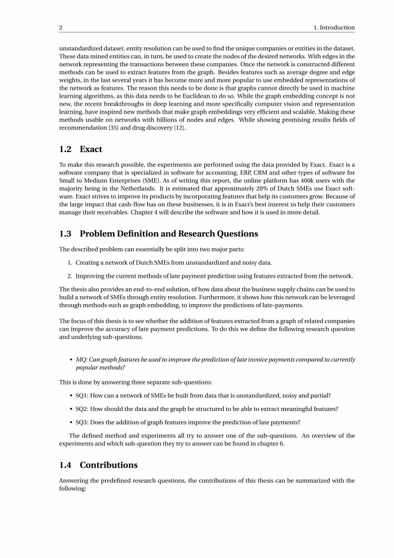
unstandardized dataset, entity resolution can be used to find the unique companies or entities in the dataset.These data mined entities can, in turn, be used to create the nodes of the desired networks. With edges in thenetwork representing the transactions between these companies. Once the network is constructed differentmethods can be used to extract features from the graph. Besides features such as average degree and edgeweights, in the last several years it has become more and more popular to use embedded representations ofthe network as features. The reason this needs to be done is that graphs cannot directly be used in machinelearning algorithms, as this data needs to be Euclidean to do so. While the graph embedding concept is notnew, the recent breakthroughs in deep learning and more specifically computer vision and representationlearning, have inspired new methods that make graph embeddings very efficient and scalable. Making thesemethods usable on networks with billions of nodes and edges. While showing promising results fields ofrecommendation [35] and drug discovery [12].

1.2 Exact

To make this research possible, the experiments are performed using the data provided by Exact. Exact is asoftware company that is specialized in software for accounting, ERP, CRM and other types of software forSmall to Medium Enterprises (SME). As of writing this report, the online platform has 400k users with themajority being in the Netherlands. It is estimated that approximately 20% of Dutch SMEs use Exact soft-ware. Exact strives to improve its products by incorporating features that help its customers grow. Because ofthe large impact that cash-flow has on these businesses, it is in Exact’s best interest to help their customersmanage their receivables. Chapter 4 will describe the software and how it is used in more detail.

1.3 Problem Definition and Research Questions

The described problem can essentially be split into two major parts:

1. Creating a network of Dutch SMEs from unstandardized and noisy data.

2. Improving the current methods of late payment prediction using features extracted from the network.

The thesis also provides an end-to-end solution, of how data about the business supply chains can be used tobuild a network of SMEs through entity resolution. Furthermore, it shows how this network can be leveragedthrough methods such as graph embedding, to improve the predictions of late-payments.

The focus of this thesis is to see whether the addition of features extracted from a graph of related companiescan improve the accuracy of late payment predictions. To do this we define the following research questionand underlying sub-questions.

• MQ: Can graph features be used to improve the prediction of late invoice payments compared to currentlypopular methods?

This is done by answering three separate sub-questions:

• SQ1: How can a network of SMEs be built from data that is unstandardized, noisy and partial?

• SQ2: How should the data and the graph be structured to be able to extract meaningful features?

• SQ3: Does the addition of graph features improve the prediction of late payments?

The defined method and experiments all try to answer one of the sub-questions. An overview of theexperiments and which sub-question they try to answer can be found in chapter 6.

1.4 Contributions

Answering the predefined research questions, the contributions of this thesis can be summarized with thefollowing:

1.5. Report structure 3

1. A novel method for entity resolution that can be used on large scale, unstandardized, noisy and partialdatasets.

2. A novel method for late payment prediction that not only combines node embeddings to improve thecurrent standard of prediction but also makes it possible to make predictions when no historical dataabout the buyer is available.

3. Demonstration of both entity resolution and late payment prediction on a use case that has not beenseen in the literature.

1.5 Report structure

The the complete outline of the report is as follows: In Chapter 2 we make an extensive review of the liter-ature surrounding the topics of entity resolution, late-payment prediction, graph embedding and analysis ofcomplex networks. We will first look at how the taxonomy is defined around these topics, their use cases, andtheir limitations. Chapter 3 will describe how the first problem of the thesis is tackled and more importantlyhow the network of Dutch SMEs is built. Chapter 4 shows how companies within the network interact duringinvoicing and how this is observed within Exact’s system. In Chapter 5 we will describe how what the methodswill be used to solve the proposed problem. Chapter 6 describes further experimentation using the creatednetwork to answer the defined research questions. Further, section Chapter 7 discusses the results gatheredfrom the experiments and Chapter 8 gives a summary and concludes the research by answering the researchquestions. Finally, in section Chapter 9 we give a series of possible additions that could benefit the researchin the future.

Chapter 2

Related Work

To be able to understand the problem further and see what the different solutions are currently available, wereview the available literature. To scope the literature we look at the different tasks a company would have totackle to be able to perform late-payment prediction based on a network of their customers.

2.1 Late payment prediction

The literature surrounding this topic shows different types of methodologies applied for customer scoringand determining whether there is a need for intervention.

Kim et al. [19] gives a taxonomy of categories where predictive models used in customer relationshipmanagement (CRM) can be divided into response models, churn prediction models, fraud detection models,and insolvency prediction/late payment prediction models. Both insolvency and late payment predictionsare a variation of the credit scoring problem, where the goal is to define a score that corresponds to the inverselikelihood of a customer to default on some type of payment. The line between the two is drawn in theapplication of the model. Insolvency prediction models are used before a service is provided to a customer,predicting whether the customer will be able to raise enough money to meet its obligations. Late-paymentprediction models are used on a more granular level, predicting when specific payments (i.e invoices) aregoing to default. While credit scoring is a well-researched topic, there has been very little research done inregards to predicting late payments.Zeng et al. [36] show how late payment prediction could be done through machine learning. This was done bygathering invoices from four different firms including 2 fortune 500 companies, which were sent to differentcompanies around the world. Next to basic invoice information such as entry date, due date and amount,the dataset also contained the delay of payment for every invoice. Ranging from 0 to more than 90 days.For this task, several decision tree algorithms are used such as PART and C4.5. Trained on the data to beable to predict the size of the delay in terms of five classes: no-delay, 1-30 days, 31-60, 61-90 and 90+ days.Zeng compares the difference between training a model for each separate firm and training one model on alldata. The author concludes that training the model on combined data from all companies gives a significantimprovement in terms of accuracy in all cases. This suggests that invoices sent by different companies (or atleast those specific four companies) share similar behavioral patterns.

Similar approach was used in [15] and [16]. Hu in [15] tested the models in two separate scenarios:

• Scenario One (Binary outcome): Predicting whether an invoice is going to be paid on time (True/False)

• Scenario Two (Multiple outcomes): Predicting whether the invoice belongs to one of four delay classes:no delay, short delay (within 30 days), medium delay (30-90 days) and long delay (more than 90 days).

The author compared the results of five different models when trained on the dataset. These models are De-cision Tree (DT), Random Forest (RF), AdaBoost (AB), Logistic Regression (LR) and Support Vector Machine(SVM). Overall, the Random Forest classifier seemed to give the best results. The most important features inboth cases were "delay ratio" and "average days of delay" of the customer.

When looking at the multiple outcome scenarios, longer delays are the worst type of delay for the busi-ness. Additionally, classifying an invoice as "no-delay" when it is actually delayed by more than 90 days isa bigger mistake than classifying it as "delayed between 30 to 90 days". To solve this and the imbalance in

5

6 2. Related Work

PaperFeature Zeng [36] Kim [19] Cheong [8] P Hu [15] W Hu [16]amount x x x x xpayment_term x x xnumber_of_paid_invoices x x x xnumber_of_late_payments x x x xratio_paid_late x x xsum_paid x x x xsum_paid_late x x x xratio_sum_paid_late x x xmean_delay x x xaverage_amount xoutstanding xaverage_amount_outstanding xoutstanding_sum_amount xaccount_manager x xbilling_cylce xintervention_count xdemographic xproducts_used x x

Table 2.1: Table showing which features have been used by different methods. Crossed cell "x" shows that the feature has been used,empty cell shows that the feature was not used.

the dataset, the authors use cost-sensitive learning. This is done by changing the weight of the cost matrix,setting higher weights for further away classes. To show that their method performs significantly better thana possible heuristic, as a point of reference both papers use the majority class as the baseline to see whethertheir methods improve compared to a weighted random guess.

An interesting insight between the papers [36] and [15], is that the datasets show similar class frequencies.In both cases, the majority class seemed to be invoices that are paid with a delay between 1 and 30 days. Withthe no-delay class being the second most frequent. In further analysis, [15] showed that there is no correlationbetween the amount invoiced and the delay of the payment. However [16], showed conflicting results. In thiscase, the amount of the invoice was the most important feature for the RF classifier.

The authors in [36][15][16] argue that to be able to predict whether a customer will pay the invoice, therehave to be two levels of features. Namely features on invoice level and customer level. Invoice level featuresconsist of information present on the invoice such as Payment Amount, Payment Term, Entry Date, Due Date,Payment Date, etc. Customer level features consist of information gathered from the history of previous in-voices. With features such as Number of paid invoices, Number of delayed invoices, Ratio of delayed invoices,Average payment term, etc. In [19] the authors make use of additional features. The dataset was provided by aKorean broadcast service company where product and demographic information is available. This informa-tion consists of the type subscriptions the customer has (i.e. cable TV, Internet, etc), how long these productshave been used and the demographic information: age and gender. Table 2.1 shows a complete overview ofthe discussed papers and the features that they use for their proposed method.

Across all papers discussed, customer level features play a major role in the prediction of the invoice. Inall cases, invoices where customer information was missing (i.e. first-time customers) showed significant lossin accuracy. Moreover [16] shows that the prediction accuracy increases as the number of invoices per personincreases.

The authors in [19] used a similar set of classifiers in addition to a two-layer Neural Network (ANN). The paperdescribes that these models are combined to, in most cases, give better results. This is done by using a simpleaverage of the prediction probabilities of all trained models. Compared to the ensemble approach, the resultsshow that RF gives the best results when it comes to individual models. The goal of the paper was to give a fairallocation of customers to the support agents. It shows that the supervised models outperform the generalheuristic rules of allocation.

While these works predicted the likeliness of a particular invoice being delayed, [8] looked at how likely acustomer was to delay payment. This subtle difference brings the method closer to the credit-scoring prob-

2.2. Financial transactions 7

PaperModel Zeng [36] Kim [19] Cheong [8] P Hu [15] W Hu [16]Classification multi-class binary/multi-class binary binary binaryLogistic Regression x x x x xNaïve Bayes xDecision Tree x x x xAdaBoost xC4.5 xPART XRandom Forest X X XNeural Networks x X xSVM x xKNN xEnsemble X x

Table 2.2: Table showing the classifiers used by the used by different methods. Crossed cell "x" shows that the model has been used, thelarger cross shows that the model gave the best results for that problem.

lem while still using invoice data to do so. The authors show that customers from smaller companies, tendto be late more in payments. Additionally, a new measure is provided to give an idea of customer "pure-ness". Where if pureness=0, the customer will always delay the payments, and if pureness=1, the customerwill always pay on time. The pureness metric is defined by the following formula:

Pur eness =W1 · number of invoices paid on time

total number of invoices+W2 · sum of value of invoices paid on time

sum of value of all invoices

Weights 1 and 2 are set manually by the user of the model to emphasize either of the ratios. The paper con-cludes shows that the ANN approach outperforms the other models provided by SAS Enterprise.

Because of the similarity between the credit scoring problem and the late-payment prediction. It is alsointeresting to look at the methodology used for those cases. Zhou et al. [40] surveys the current state ofthe art of credit-scoring. Besides the general supervised learning methods that are also used in late-paymentpredictions such as LR, DT, and RF. There are also unsupervised and semi-supervised methods used for creditscoring. The unsupervised method that is highlighted by the paper is the K-Means algorithm. The benefits ofthe unsupervised methods are that there is no need for labeled data, which often is hard to come by.

To summarize, table 2.2 shows an overview of the papers on late-payment prediction and the algorithmsthat were used for their problem.

2.2 Financial transactions

Financial transactions can be modeled as a dynamic graph to analyze the interaction between different finan-cial bodies. Work done by [33] explores different types of metrics in an economic system model as a complexnetwork. The network explains monetary transactions between 105 clusters, each representing an economicactivity standardized by the UN. The paper provides the following two contributions: A Network definitionthat is as follows:

• Node, is an economic activity cluster, with the node weight being the summed transactions within thecluster.

• An undirected Edge is present when money flows between two sectors. Its weights show the summedmoney flow between two clusters in either direction.

The paper applies different metrics (such as the distribution of degrees and correlations between neighbors)to find the following insights:

• Activity clusters with a large internal flow tend to cooperate with many other clusters via high volumemonetary transactions.

8 2. Related Work

• Activity clusters with a lower internal transaction volume prefer to transact with fewer neighboringnodes that have a higher internal flow.

• The node weights seem to follow a power-law distribution.

• Activity clusters tend to balance the monetary volume of their transactions with their neighbors, re-flected by a positive link weight correlation around each node.

Graph-based approaches are also used in the domain of risk assessment and fraud detection. [22] showsan example of how graph-based semi-supervised learning can be used to improve an existing fraud detectionsystem. The authors highlight that in networks of transactions, the presence of hubs can harm the fraudclassifier. These hubs are nodes with a high degree and thus neighbors to a large number of nodes. As thesenodes accumulate a large number of transactions, they tend to accumulate a large amount of risk score. Tosolve this issue the risk scores are normalized by the node degree.

2.3 Graph analysis and feature engineering

Graph embedding methods have seen a spike in interest and application in the last couple of years. Thesegraph embeddings make it possible to encode graphs, making it possible to use graphs as input in variousmachine learning algorithms. This was previously not possible due to the non-Euclidean nature of graphs.Besides embedding, the most basic way to represent a graph is by encoding it as an adjacency matrix. How-ever, as every row only contains information of the neighbors of a single node, adjacency matrices are a verysparse and thus inefficient representation of the graphs. Within these matrices, there is no notion of similar-ity if two nodes do not share any neighbors or labels. Preferably, we would like to have an embedding thatlets us compare nodes (or other aspects of graph structure) that are far from one another. Representationsgathered from graph embedding make this possible.

The concept of graph embedding itself has been present for decades and closely associated with dimen-sionality reduction. In dimensionality reduction the goal is to represent a n x m matrix as a n x a matrix,where a << m. While dimensionality reduction is beneficial, in representation learning it is not required.The goal of the representation is to map the graph to a latent space that makes the information used for othertasks, even if the dimensionality does not decrease. Works such as [34], [7], [39], [6] have surveyed the dif-ferent graph embedding methods, describing their benefits, limitations, and taxonomies categorizing them.The surveyed works show examples of graph embedding being used in tasks such as classification, clustering,link prediction, anomaly detection, and visualization. The embedding methods can encode a complete graphor different parts of the graph to a set of vectors. Based on the output granularity, the embedded output canbe divided into four different output types. Namely node embedding, edge embedding, hybrid embedding,and graph embedding. The type of output depends on the desired application and the embedding algorithmthat is used.Generally, the embedding algorithms are categorized by its method:

• Matrix Factorization: the embedding is achieved by factorization of the adjacency matrix.

• Random Walk based Deep Learning: uses the SkipGram architecture to learn effective embeddings ofrandom walks generated from the graphs.

• Non-Random walk Deep Learning: these methods leverage network architectures such as autoen-coders or graph convolution layers to embed the input.

In the next few segments, we will take a closer look at the different types of graph embeddings and theirapplications.

DeepWalk [29] was the first to use random walks in combination with the SkipGrams to embed nodes intoa latent space. SkipGram is a language model that maximizes the co-occurrence probability among the wordsthat appear within a sentence. The DeepWalk method argues that random walks in a graph, starting from aseed node, can be seen as sentences of nodes. These sentences are used as context for the SkipGram model,optimizing the co-occurrence of neighbor nodes in the walk. As the number of nodes in these networkscan increase to million or in some cases even billions, the softmax layer of the SkipGram is replaced by aHierarchical Softmax layer. Instead of predicting the isolated individual nodes, the problem is turned intomaximizing the probability of traversing a specific path in a binary tree. Within this binary tree, the leaves are

2.3. Graph analysis and feature engineering 9

the individual nodes of the network. This reduction of the output layer significantly reduces run-time, with aslight reduction in accuracy as a trade-off. Once the training is done, the output layer is removed, leaving theinput layer and the embedding layer. The remainder of the model can be used to embed any arbitrary nodefrom the network. Following the introduction of DeepWalk, works of LINE [32] and Node2Vec [13] showedimprovements in terms of random walk strategy and alternatives for Hierarchical Softmax.

Node2Vec [13] provides an extension to the framework of DeepWalk [29] by introducing a biased methodof a random walk. According to the authors, nodes within a graph can share similarities based on the follow-ing two aspects:

1. Nodes that are highly interconnected and belong to similar network clusters or communities should beembedded closely together (homophily)

2. Nodes that have similar structural roles in networks should be embedded closely together (such ashubs, bridges)

Unlike homophily, nodes with structural similarity do not have to be closely connected. real-world networksoften show both of these equivalences among similar nodes. To find these similarities there needs to be atrade-off between exploring the network in the search for structurally similar nodes, but also exploring thedirect neighbors that possibly belong to the same community. To be able to benefit from these aspects, theauthors introduce a bias into the random walk that increases either exploration or exploitation.Random Walk methods have been one of the first scalable methods that have been available for graph em-bedding of large graphs. However, more recently deep learning methods have been becoming more popularin the literature. This is due to the success achieved by the work done in deep neural network architec-tures such as Convolutional Neural Networks (CNNs). One of the first attempts to make the convolutionkernel generic enough to be applicable for graph-structured and 3D data was done using spectral convolu-tions [4]. While very promising, the spectral graph convolution requires the computation of the eigende-composition of the graph laplacian. The theoretical complexity of the decomposition is equivalent to thecomplexity of matrix multiplications. With a naive method, this can be done in O(n3). Methods such as theCoppersmith–Winograd algorithm [10] can reduce the time to O(n2.373). However, even with this speedup,the method quickly becomes expensive if the size of the graph is increased. Work that was done in Kipf et al.[20] shows that the graph convolutions can be done in linear time and used for semi-supervised classificationto propagate node labels. This method is similar to the Weisfeiler-Lehman algorithm where the hashing stepis replaced by the convolution. One of the important contributions of this work is that the graph convolutioncan now be used on large graphs and even run on GPU’s. This greatly reduces the run-time compared to therandom walk method which cannot be run in parallel. The graph convolution method has some limitationsin terms of application. For example, the embeddings do not take into account the direction of the edges, northe weights of the edge.

The graph convolution operator has sparked a new set of neural networks and is defined by the literatureas Graph Convolutional Networks (GCN) or Graph Neural Networks/Geometric Neural Networks (GNN). Anexample of its use is work done by Monti et al. [26]. The paper describes how cascades of twitter retweetscan be used to predict whether a website contains fake news. Cascades are subsets of the social graph. Ev-ery cascade contains the propagation of the information (in this case tweets containing URLs) after severaltimesteps. Monti et al. propose a model that takes a cascade information as input in the form of a graph anduses two graph convolution layers in combination with pooling to predict weather the retweets contain fakenews.

After training the network, the output from the second convolution layer is visualized with t-SNE. Thevisualization in fig. 2.1 shows that the learned features clump together samples of the same class.

The choice of embedding method depends on the task at hand. When it comes to comparing the RandomWalk methods to the GNN’s, the biggest difference between the two is that while Random Walk is optimizedfor representation, the GNN methods are end-to-end and thus are optimized for the task at hand. Arguably,the end-to-end methods should result in more accurate models since it is directly optimized for that. How-ever, the benefits of learning a representation is that it can be done completely unsupervised. This meansthat there is no need for labeled data (which often is not present and costly to get) or a model to be trained toachieve the embedding.The discussed methods are still a major topic for research. Cai et al. [6] categorize different problem set-tings, graph embedding methods shown in the field and, analyses the advantages and disadvantages of thesemethods. The author describes the four research directions for the fields of graph embedding:

10 2. Related Work

Figure 2.1: t-SNE representation of the features before the classification layer.

• Computation. The deep architecture, which takes the geometric input (e.g., graph), suffers from alow-efficiency problem. Traditional deep learning models (designed for Euclidean domains) utilizethe modern GPU to optimize their efficiency by assuming that the input data are on a 1D or 2D grid.More work is needed in researching how to be able to use GPU’s for graph input data.

• Problem setting. Existing graph embedding mainly focuses on embedding the static graph and the set-tings of dynamic graph embedding are overlooked. How to design effective graph embedding methodsin dynamic domains remains an open question.

• Techniques. Current edge reconstruction based graph embedding methods are mainly based on theedges only. The global structure of a graph (e.g., paths, tree, subgraph patterns) is omitted. Intuitively,a substructure contains richer information than one single edge. An efficient structure-aware graphembedding optimization solution, together with the substructure sampling strategy, is needed.

• Applications. It is of great importance to exploring the application scenarios which benefit from graphembedding, as it provides effective solutions to the conventional problems from a different perspective.

2.3.1 Feature engineering

Since networks cannot directly be used as input in machine learning models. The problem of prediction re-lies primarily on the quality of engineered features. Therefore, it is important to have effective techniquesthat extract meaningful features from the networks. A well-known problem in this domain is the problem oflink prediction, where the goal is to find missing links in a network using information about the nodes. Mutluet al. [27] shows a taxonomy of the graph features primarily used for link-prediction (fig. 2.2). In addition tothis taxonomy, works such as [23] that structural features such as graphlets can be viable depending on theproblem domain.

Promising work by Zhang et al [38], shows that the combination of several techniques can be very beneficial.The authors show that the graph structure features such as Katz index, rooted PageRank and SimRank aredifferent from the latent features learning with graph embedding methods. With this insight, a new frame-work is proposed named SEAL. The framework uses three types of features to predict the likelihood of a linkexisting between two nodes. The used features come from: a GNN method called DGCNN, embedding made

2.3. Graph analysis and feature engineering 11

Figure 2.2: Taxonomy for the feature extraction techniques and feature learning methods for link prediction studies.

Figure 2.3: List of heuristic features used by the SEAL model for link prediction.

12 2. Related Work

by node2vec and a list of heuristics that can be seen in fig. 2.3. The paper shows that the information from dif-ferent types of features gives an increased generalized performance. With the use of heuristic features alone,in some cases, the model performed at a similar accuracy as a random guess.

2.4 Entity Resolution

Entity Resolution (ER for short, also known as Entity Matching, Entity Disambiguation, Record Linkage) de-scribes the problem of finding unique entities from either single or multiple data sources [31]. The paperdone by Konda et al. [21] describes that while there has been an effort made in understanding the problemthere is very little to no published work on ER in practice, end-to-end. The general outline of the paper is toshow the methodology and workflow of doing ER in a real-world scenario. It argues that every unique caseneeds experts to differentiate the records and heuristics. The paper contributes a description of a real-worldapplication, the goals set by the stakeholders involved and a description of the common ER challenges inreal-world applications.

The authors describe the first step to be setting up the matching rules:

1. Two records are a direct match if the unique ID is the same in both records.

2. If Titles are similar.

3. If similar individuals are involved.

The second step is blocking. In this step, candidate matches are excluded based on some rules. Theserules are in this case heuristic thresholds. After the candidates were made, the data were manually labeledby a trained student (only 300 matching pairs were labeled). Train several Sci-Kit learn [28] classifiers untilthe best one was found. The author describes non-matching rules, to be rules that when true remove thecandidate. Similar to blocking. The paper argues that the best method for ER would have a combination ofML and rule-based methods as matches.

In Chapter 3 we will further look into Entity Resolution and how it is used on the data provided by Exact.

Chapter 3

Entity Resolution

As previously mentioned one of the goals of the proposed framework is to create a network of Dutch SMEsthat can be used for further network analysis and feature extraction. The way this is going to be tackled isby proposing a tailored method for recognizing unique companies in the data and building relationshipsbetween them. In the next sections, we will take a closer look into how the data of the accounts are set up,what the challenges are in building the network of companies, and how the proposed method tackles them.

3.1 Division-Accounts

With the software suite from Exact, companies and accountants can do their bookkeeping digitally. This andmany other functionalities fall under the cloud solution, Exact Online (EOL). Within the EOL framework, thereexist three levels of accounts. Level 1, the upper level, also called the Account, refers to a single license thatan entity has purchased to be able to use the software. A single license contains administrations of severalcompanies. For example, an accountant can purchase a license to do the bookkeeping for multiple admin-istrations. These administrations are considered level 2. A single administration or division is a single entitythat has its bookkeeping done in the system. These businesses have a collection of (Division-)Accounts whichare other business entities they do business with. Depending on the business these can be either companiesor any other private customer. With almost 400,000 unique divisions, the majority of these companies are sit-uated in the Netherlands. This segment covers roughly 20% of the dutch SMEs. As this is a major segment ofthe Dutch market, there is a high probability that if a division sends an invoice to a company, and it happensto be an SME, that it is an administration in EOL. However, to be able to recognize that this is indeed the case,the available information needs to be cross-compared to the accounts in the dataset. To see how this can bedone, we look at what type of information is available with each account.Following this, level three will be referred to as Accounts or Division-Accounts, level two will be referred to asDivisions or Administrations and Level one will be referred to as Licenses.

In the following sections, we will look at how we can solve the deduplication problem in a dataset thatcontains noisy unstandardized data. The problem of deduplication is a special case of record linkage. Whereinstead of linking several datasets together, records that represent a single entity within a single dataset aregrouped. The goal of deduplication is to transform a dataset containing duplicate records to a smaller datasetcontaining all unique entities. Which in this case are Dutch SMEs.

3.2 Problem of record matching

Data has been the crude oil of the twenty-first century and has been the driving force behind the changes inhow companies service and do business in general. However, clean structured data is often very hard to comeby. Especially when it comes to SMEs, which often do not have designated data science roles. Moreover, theneeded data is often spread over different sources and needs to be integrated so that can be used to generateuseful insight. Of course, these data sources often come from different parties or vendors, are unstandardized,noisy and partial. By some [1], the problems of data integration and approximate data deduplication areconsidered as the biggest problems in the world of data.

13

14 3. Entity Resolution

Figure 3.1: Generic pipeline of ERA

The data provided for this project was a dataset containing divisions(customers of Exact) and all of theiraccounts. Every account contains information of one or more companies/persons that division is doing busi-ness with. As this information can come from various sources, the data is not standardized and in most casesis incomplete. Two divisions can do business with the same supplier but have different information in almostall fields of the account. For example, the given name strings could look like one of the following: "AlbertHeijn", "Albert Heijn | Allerhande Kookt", "AH" or "Alfred Heijn". Looking at the company names, if one hasheard of Albert Heijn it would be easy to distinguish the four cases from each other. This is because we knowwhat the abbreviation stands for and we are familiar with other aliases that the company has. However, it isvery difficult to do this fully automatically. Besides, there are different types of information that could to betaken into account, such as address and other account details. To get a complete picture of which recordsare similar to each other, one would have to cross-compare all available records. While this possible for smalldatabases, cross-comparison quickly because impossible when the sets grow to millions or billions in size.Another method would be to use a clustering algorithm that groups records together that a similar based onsome metric. However, the time complexity of algorithms such as DBSCAN is quadratic in the worst case,and thus unscalable for datasets of millions. Without even considering the difficulty of defining the similaritymetric for the task. To make the matching algorithm scalable and effective, there needs to be series filters andoptimizations that avoid making extra comparisons. To give an overview of these steps, the next section willdefine the pipeline for resolving entities.

3.2.1 Generic ERA pipeline

Rahm et al. [31] give a generic overview of how an Entity Resolution Algorithm(ERA) looks like if it generalizedas a pipeline of steps. This can be seen in fig. 3.1

A generic ERA method achieves final clustering of records about the same entity using the following steps:

1. Preprocessing: in the first step of the pipeline, the records are standardized and cleaned as much aspossible to make the following steps easier to achieve. This can be simple sanitation or simplificationof input using domain knowledge.

2. Blocking: as cross-comparison is not possible if the dataset is large enough, records are pre-groupedin blocks or clusters. Once this is done, records inside the block are then cross-compared. The benefitof this is that the comparison is only done on records that already have something in common. Forexample, a block could be all records that have a specific postal code.

3. Similarity comparison: In this step, different similarity metrics are calculated to create sets of features.These are used in further steps to distinguish matching from non-matching records. An example ofthese features is the edit distance between two names.

4. Classification: Once the features are made, a classifier is used to find the matching records. This classi-fier is trained beforehand using a dataset that is defined for this specific task.

5. Clustering: Once the records are compared and classified, it is important to have a strategy that clustersthe records into specific entity clusters. This is needed because records can match to several differentrecords or entities. Especially when the data is noisy, this can be a major problem. The clustering makessure that there is a split in groups of records that all belong to a specific entity. Without this final step,the entity groups implode to a small number of entities.

3.2. Problem of record matching 15

As previously mentioned, one of the biggest problems with entity resolution is that no one solution fits allcases. This is primarily because generic methods don’t scale to larger sizes of the dataset. This often dependson the approach to be tailored for the problem at hand. While there has been work done on ER on publicdatasets, there has been little work done on ER in practice. Because of this, a custom ERA method has beendeveloped to find the unique groups of records within the data of Exact.

In further sections of the chapter, the focus will be on how the data is constructed and what steps aretaken to build a graph of Dutch SMEs using a tailored ERA method.

3.2.2 Data definition and preprocessing

Before we go into the further steps, we look at how the data is defined and how it is pre-processed. Everyaccount consist of the following information:

• Name: The name of the organization or person. (Required)

• Address: The address at which the organization or person resides. It can also be a registered mailbox toreceive mail. (Optional)

• Postal code: The postal code of the address. It can also be the Postal Code of the mailbox. The combi-nation of the postal code and address number is unique. (Optional)

• Email: The email address of the organization. It can also be the email address of a contact person in thecompany. (Optional)

• Phone: Phone number of the organization, support line or contact person. (Optional)

• Website: Website of the organization (Optional)

• Chamber Of Commerce/Kamer van Koophandel (KvK): This is a unique identifier that every companyin the Netherlands has (Optional).

• VAT Number: Identifier used for tax filing, also unique in the same manner that KvK is. (Optional)

• IBAN: Bank account number of the organization (Optional).

Importantly the user of the system does not have to fill in any of the fields except for the company name.Unfortunately, while key fields such as KvK and VAT are very useful when matching accounts together, theyare only present in a small fraction of the accounts. Figure fig. 3.2 shows the number of records that containa value in the presented fields.

As can be seen in the figure, only roughly 12% of accounts contains a KvK number, and even less has aVAT number. When we compare these two sets, we can see that while there is a lot of overlap between theseaccounts. Figure 3.3 shows the relationship between these sets.

However, we can see that if we group records by their respective KvK number, the majority of the groupshas multiple VAT numbers among the clustered records. While having (had) different VAT or KvK numbersfor one specific company is possible, because of the change in ownership, this makes it hard to group recordsby a single value. Even more so because the input information is not standardized by any method and iscompletely up to the user.

The first step of the pipeline is the preprocessing step. During this step, we try to filter out as many unus-able accounts as possible and standardize as many of the values as possible to make our life easier in furthersteps. For example removal of characters that are not used in the alphabet and more specifically, noisy terms.As a large number of these accounts are names of organizations, they often have their legal status in theirname. For example My Company LLC. The LLC, in this case, describes that the organization is a Limited Lia-bility Company, similar to a BV and VoF in the Netherlands. Whether or not these terms should be removeddepends on further methods of comparison. While the legal status gives useful information in terms of con-text, similarity metrics that look at overlap in characters will find similarities only because the companiesshare the same legal status. As we are using such metrics, as will be explained in further sections, the legalterms have been removed from the account name. If use case and memory permits, it is possible to extractthe legal status from the name and use it in further steps or other applications. However, in our case, thisinformation was taken out to keep the columns in the dataset as manageable as possible.


Figure 3.2: Overview of how many fields of the given accounts have been supplied with information.

Figure 3.3: Overlap between KvK and VAT.


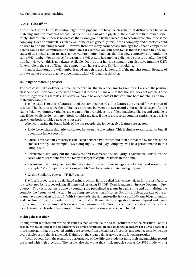
3.2.3 Classifier

At the heart of the Entity Resolution algorithms pipeline, we have the classifier that distinguishes betweenmatching and non-matching records. While being a part of the pipeline, the classifier is first trained sepa-rately. Unfortunately, there is no dataset that shows ground truth of whether to accounts are about the samecompany. KvK and similar IDs such as VAT number are generally unique for a company, and therefore couldbe used to find matching records. However, there are many corner cases and legal tools that a company orperson can do that complicates the situation. For example, an issue with KvK is that it is person bound. Be-cause of this, when a person starts a new venture it often happens that this new company is put under thesame KvK number. For this specific reason, the KvK system has another 2 digit code that is put after the KvKnumber. However, this is not always available. On the other hand, a company can also have multiple KvK’sfor example in the case of Exact, the company can have a second KvK for its holding.

In most situations, the KvK number is good enough to get a large chunk of the matches found. Because ofthis, we can use records that have been made with KvK to train a classifier.

Building the matching dataset

The dataset is built as follows: Sample 1M record pairs that have the same KvK number. These are the positiveclass samples. Then sample the same amount of records but make sure that the KvK does not match. Theseare the negative class samples. This way we have a balanced dataset that contains both matching and non-matching examples.

The next step is to create features out of the sampled records. The features are created for every pair ofrecords. The features show the differences in values between the two records. For all fields except for theName field, two dummy variables are created. First variable is true if field matches. The second variable istrue if the two fields do not match. Both variables are false if one of the records contains a missing value. Thecase where both variables are true is not used.

When comparing the Name fields of the two records, the following five features are created:

• Ratio, Levenshtein similarity calculated between the two strings. This is similar to edit-distance but alloperations have a cost of 1.

• Partial, Levenshtein similarity is calculated between two strings and then normalized by the size of thesmallest string. For example: "My Company BV" and "My Company" will be a perfect match in thiscomparison.

• Levenshtein similarity but the names are first lowercased the similarity is calculated. This is for thecases where users either use too many or forget to capitalize letters in the name.

• Levenshtein similarity between the two strings, but first these strings are tokenized and sorted. Forexample: "My Company" and "Company My" will be a perfect match using this metric.

• Cosine Similarity between TF-IDF vectors.

The first four features are calculated using a python library called fuzzywuzzy [9]. As for the last feature,it is calculated by first vectorizing all name strings using TF-IDF (Term Frequency - Inverse Document Fre-quency). The vectorization is done by counting the predefined n-grams in each string and normalizing thecount by the frequency of the term in the complete collection of strings. For this problem, the size of the n-grams have been taken to 1 and 2. With 2-size words, the dimensionality is close to 1400. Any bigger n-gramsand the dimensionality explodes to an unpractical size. To keep this manageable in terms of speed and mem-ory, the size of the n-grams had been kept to a maximum of 2. Once this is done, the dataset is ready to beused to train the classifier. An example of how the features look can be seen in fig. 3.4.

Picking the classifier

An important requirement for the classifier is that we reduce the False Positive rate of the classifier. For thisreason, when looking at the classifiers we optimize for precision alongside the accuracy. For our use case, it ismore important that the created entities are created from a clean set of records, and not necessarily includeevery single record that is matched. Training on the created dataset, we get the following results:

As can be seen from the results the performance of the different models is fairly high and matching recordare found with high precision. The results also show that the simple models such as the SVM model with a


Figure 3.4: Example of the matching dataset used to train the matching classifier

RandomForestClassifier DecisionTreeClassifier LinearSVCAUC 0.97350 0.95693 0.97113Accuracy 0.97350 0.95693 0.97113Precision 0.98721 0.95341 0.99673

Table 3.1: Performance of several classifiers on the matching dataset.

linear kernel perform similar to the model complex models such as the Random Forest. A closer look at thefeature importances and specifically the cosine similarity between the tf-idf vectors show that the majority ofthe non-matching are easily found.

Figure 3.5 shows a small sample of 250 matching and non-matching examples. By taking the cosine sim-ilarity and putting it against the partial similarity, we can see that the two classes are fairly easily separable.Because of this and precision of the model, we have taken SVM as the go-to model for match classification.

3.2.4 Custom method for Entity Resolution

As mentioned earlier a general ERA contains the following steps: preprocessing, blocking, classifying andcombining. In the following section, we will describe the proposed ERA by going through the steps it takes todisambiguate the entities.

Intuition

The algorithm is specialized and optimized for the dataset at hand. The method was created with specificheuristics in mind. In our case, we know that there are several IDs or keys that can be used to group records.What about when multiple keys are available? Can we leverage the existence of these keys for a fast andscalable implementation of ER? Theoretically, with the use of multiple keys to compare with, the providedentities should be less noisy compared to the mappings made with a single key alone. In further steps, welimit the available data to a segment of the accounts that have either a KvK, VAT or IBAN number. We takespecifically these accounts because we are interested in the companies within the collection. The accountsthat do not have these values are often private accounts and don’t belong to an organization.

Method

As Name is the only mandatory field, there is a large number of records that have a very limited amount offields filled in. When cross-comparing these records, there is a lot of uncertainty in the comparison due tothe sparsity. Because of these matches are often misclassified. For example, what is common among SMEsis change of branding or maybe even ownership. Especially since the data start in 2005 it is likely that thishappens over time. So if one would take two records and try to compare them to each other, it is possible thatone of the accounts holds the new brand name of the company, while the other one does not. Due to missinginformation, this could result in a non-match. However, it is possible that other accounts that belong to thatsame cluster, have the fields that can be used to match with the candidate. Generally, this is handled by crosscomparing records within a block. However, if the size of the block gets bigger, it quickly becomes unscalable.In this method, the comparison is made by comparing the record the mode of the collection. The mode of acollection contains the most common value in a field in all of its fields. However, this is not always possible.For example, if one of the fields does not have a single value that is most common, but multiple that occurthe same amount of time. In this case value for the field is taken at random, from one of the common values.


Figure 3.5: Scatter plot of matching and non-matching records, with on the x-axis the cosine similarity between the two strings and onthe y-axis the partial similarity.

Step1: Initial groupingIn the first step of the algorithm, a choice is made of which fields to use for clustering. These can be anycolumn of the dataset. Once the fields are chosen, buckets are made for each unique value or key from thesecolumns. It is important to note that records are put in multiple buckets if more than one of the columnscontains a value. In our case, we choose to use KvK, VAT, and IBAN as fields to group on. Once the initialgroups are made, a single record is created from the mode of the collection that represents that group, similarto a centroid in the K-Means algorithm.

Step 2: Flagging similar clustersOnce the first set of clusters and its modes are created, the next step merges clusters that are similar to eachother. This is done using the classifier that is trained beforehand and instead of cross-comparing all records,only the modes of the clusters are compared to each other. If this record pair is matched then the clusters areflagged to be merged. The goal of the merging step is to reduce the number of total clusters and to optimizethe blocking step by matching groups of records together instead of doing so one by one. To further optimizethe number of matches that need be made only candidate clusters are compared to each other. Candidatepairs are found by looking at whether there are any overlapping records.

Step 3: Combining matched clustersOnce the matching clusters have been flagged, a merging strategy needs to be applied to segment the matchesand re-cluster them. This is done by creating a graph of the clusters and connecting clusters with one anotherif they have been matched in the previous step. Applying any community search algorithm on this graph willsegment the clusters into communities where each community represents a collection of records of an entity.However, to avoid merging long chains of matches and other types of loosely connected communities, thealgorithm combines clusters that belong to the same maximal clique. Meaning that clusters are only mergedif all clusters in a segment match with one another. Once this step is done the number of clusters is generallyreduced by a large amount. However, for every cluster pair that didn’t match, a set of records exist that are inmultiple clusters.

Step 4: Remove multi-dippingIn this step, duplicate records are removed and made sure that they only are placed in one cluster. This isdone by comparing the record to the modes of the clusters it belongs to. The record is then removed from


Figure 3.6: Distribution of similarity between the mode of a cluster and the inner records. Clusters smaller than 5 have been takenfiltered out.

all clusters except for the one where the classifier gives the highest softmax probability. Once the final step isdone, the results are clusters of records where to contents of each cluster belong to a single entity.

Results

To benchmark the proposed method, we compare the created entities to a baseline method of grouping ac-counts, which is grouping them on the provided KvK. While the proposed method works on a larger set ofdata and does not necessarily need KvK specifically to match records together. To make the two methodsmore comparable, the data is limited to the accounts that have a KvK number. The following results showthe comparison of a baseline (records grouped on KvK) and the proposed method using two heuristics. Thefirst heuristic shows the distribution of the similarity between the mode of a cluster and the records that arewithin it. The second heuristic shows the fraction of records that have a specific amount of modes within itscluster. A larger mode length means that there are no values that are prevalent in the cluster. If many of therecords are the same, specific values of the cluster will make the majority of that cluster.

As can be seen from fig. 3.6 and fig. 3.7, for both heuristics the proposed method outperforms the base-line. However, with these heuristics, it is hard to say whether the pureness of the clusters actually improveswhen the proposed method is used. Because of this, further experimentation was conducted to research thepureness of the clusters as a subjective measure when evaluated by human subjects. How the experimentwas conducted exactly can be read in Appendix A with the briefing that was used to explain the problem tothe subject in Appendix B.

In short, the experiment was done by showing Exact fields experts samples from clusters made by the pro-posed algorithm the baseline. The subjects would not know what method was used to group the records. Theexperts would be asked to label records they think were grouped incorrectly. This is done for roughly 24 clus-ters. With 10 records per cluster and the clusters equally split, the subject labels 120 records for each method,resulting in 240 records per subject. The results of the questionnaires have been aggregated in fig. 3.8a andfig. 3.8b. Figure 3.8a shows the number of defects that each of the subjects has found in its questionnaire.Looking at the number of defects per category shown by fig. 3.8b it seems that in some the preferences be-tween the methods vary between subjects. However, having asked the subjects whether they were able topredict which questions were generated by which method. None of the subjects were able to consistentlypredict which was which and generally saw no difference between the questions. The same could be saidfrom looking at the statistics. Figure 3.9 shows the contingency matrix of the experiment. As can be seenfrom the matrix, the difference between the two methods is very small in comparison. The proposed methodonly has several defects less than the baseline. To see whether this difference is significant we perform a


Figure 3.7: Fraction of the clusters that have a certain amount of possible modes. Clusters smaller than 5 have been taken filtered out.

(a) Defects and non-defects per subject (b) Amount of defects per category


Figure 3.9: Contingency matrix of the experiment

Chi-square test. With a p-value > 0.05, the difference between the two seems to be insignificant.

Chapter 4

Invoicing

An invoice is a document issued from the seller of goods (or services) to the buyer. This document containsinformation about the purchase. Such as the amount that is owed, a payment deadline and sometimes ashort description of what is that is being sold. There exist two types of invoices: Sales Invoices and PurchaseInvoices. This type depends on the perspective of the user. When a division is buying goods, this is registeredas a purchase invoice into the system. In the case of selling goods, the invoice would be registered as a Pur-chase Invoice. The Invoices table contains all individual sales invoices sent from individual divisions to theircustomers. Every record contains several pieces of information about the invoice, such as the amount paidand the payment term. As these invoices are historical, they include information about when the actual pay-ment has taken place. However, this information is not always available. The invoices and the correspondingpayments need to be registered manually. Most common is that this information is put in by either a com-pany administrator or accountant into the system. Figure 4.1 shows the possible interactions between thedivision, its customer and the bookkeeping system where the data is stored and processed.

The figure shows that there is an exchange of information between the sender and the receiver. All ofthe data is put into the system by the user and the user can do this whenever he/she desires to do so. Theseinteractions don’t have a specific order and are not enforced on the user in any way. Moreover, as thesepayments are not done automatically, there is a discrepancy between the state of the system (informationavailable) and the actual situation. Resulting in the system to show an outstanding invoice, while in actualityit has been paid and not yet registered.In any case, the following information about an invoice can be available:

• Amount: The amount to be paid by the customer.

• Division ID: Identifier that belongs to a single division in the system.

• Division Account ID: Identifier that belongs to a single Division Account.

• Invoice ID: Identifier that belongs to a unique Invoice.

• Entity ID: Unique Entity ID inferred from the Entity Resolution algorithm.

• Due Date: The deadline at which the payment from the buyer has to be received by the seller.

• Invoice Date: The date that describes the beginning of the payment term. Generally, this is the datewhen the buyer receives the invoice.

• Payment Term: The number of days that the user has to pay the invoice. Calculated by counting thenumber of days between the invoice date and the due date.

• Payment Date: the date at which the seller has received the payment from the buyer.

• System Invoice Date: The date at which the invoice has been entered into the system.

• System Payment Date: The date at which the invoice has been entered into the system.

• Is Late: whether an invoice was paid late. Invoice is late if the Payment Date is bigger than Due Date.The target for the machine learning models.

23

24 4. Invoicing

Figure 4.1: Interactions between the Division (in the illustration the Invoice Sender) and one of their accounts (Invoice Receiver in theillustration) in no specific order.

• Payment Delay: The number of days that the invoice is paid late. Step-function where the delay is thenumber of days from Due Date to Payment Date. Delay is 0 if payment was on time.

By looking at the most frequent date sequences, we can define a general case. This can be seen in fig. 4.2. Thetop 10 covers over 90% of all invoices. As can be seen, the invoice date (I ) is the first date in the majority ofcases. This means that most of the time the invoice is received before it is put into the system.The most frequent sequences seem to correspond with the following chain of events:

1. The invoice is created by the seller of the goods and sent to the buyer.

2. This invoice is entered by the seller into the system as a sales invoice that has been sent to one of theaccounts.

3. The buyer receives the invoice and pays this at a certain moment in time.

4. Once the payment has been received by the division, this is entered into the system either manually orsome type of import method.

Further analysis over the complete dataset shows that it is the case for 97.7% of the invoices. For the remaining2.3%, the order at which information becomes available is very different. For example, for a segment of theinvoices, the payment is done before the invoice date. Resulting in a negative days-outstanding. In othercases, an invoice is registered into the system way ahead of time. An option would be when the seller has asubscription-based business model. In other cases, it is even possible that a buyer has paid for somethingahead of time. The following section will focus on exploring the data through an EDA.

4.1 EDA

In this section of the chapter, we will explore the dataset to gain insight into the problem. This gained insightshould help us make design decisions in further steps. During the EDA of the invoice, we look specifically forthe following aspects of the dataset: The distribution, time-line, class balance and returning customers.

4.1. EDA 25

Figure 4.2: Barplot shows the most frequent sequences of dates in the system. The sequences have been coded for readability (InvoiceDate = I, Payment Date = P, System Invoice Date = Is, System Payment Date = Ps,). The sequence next to a bar represents the order of the

dates. Leftmost symbol is the oldest date, rightmost the most recent. Two symbols in brackets are equal, in other words these datesrepresent the same day.

(a) Sent. (b) Received.

Figure 4.3: Distribution of invoices sent and received by the divisions. Only shows divisions with counts from 1 to 25 invoices.

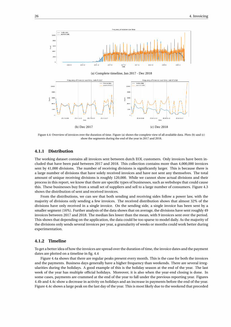
26 4. Invoicing

(a) Complete timeline, Jan 2017 - Dec 2018

(b) Dec 2017 (c) Dec 2018

Figure 4.4: Overview of invoices over the duration of time. Figure (a) shows the complete view of all available data. Plots (b) and (c)show the segments during the end of the year in 2017 and 2018.

4.1.1 Distribution

The working dataset contains all invoices sent between dutch EOL customers. Only invoices have been in-cluded that have been paid between 2017 and 2018. This collection contains more than 4,000,000 invoicessent by 41,000 divisions. The number of receiving divisions is significantly larger. This is because there isa large number of divisions that have solely received invoices and have not sent any themselves. The totalamount of unique receiving divisions is roughly 120,000. While we cannot show actual divisions and theirprocess in this report, we know that there are specific types of businesses, such as webshops that could causethis. These businesses buy from a small set of suppliers and sell to a large number of consumers. Figure 4.3shows the distribution of sent and received invoices.

From the distributions, we can see that both sending and receiving sides follow a power law, with themajority of divisions only sending a few invoices. The received distribution shows that almost 32% of thedivisions have only received in a single invoice. On the sending side, a single invoice has been sent by asmaller segment (16%). Further analysis of the data shows that on average, the divisions have sent roughly 49invoices between 2017 and 2018. The median lies lower than the mean, with 9 invoices sent over the period.This shows that depending on the application, the data could be too sparse to model daily. As the majority ofthe divisions only sends several invoices per year, a granularity of weeks or months could work better duringexperimentation.

4.1.2 Timeline

To get a better idea of how the invoices are spread over the duration of time, the invoice dates and the paymentdates are plotted on a timeline in fig. 4.4

Figure 4.4a shows that there are regular peaks present every month. This is the case for both the invoicesand the payments. Business days generally have a higher frequency than weekends. There are several irreg-ularities during the holidays. A good example of this is the holiday season at the end of the year. The lastweek of the year has multiple official holidays. Moreover, it is also when the year-end closing is done. Insome cases, payments are crammed at the end of the year to fall under the previous reporting year. Figures4.4b and 4.4c show a decrease in activity on holidays and an increase in payments before the end of the year.Figure 4.4c shows a large peak on the last day of the year. This is most likely due to the weekend that preceded

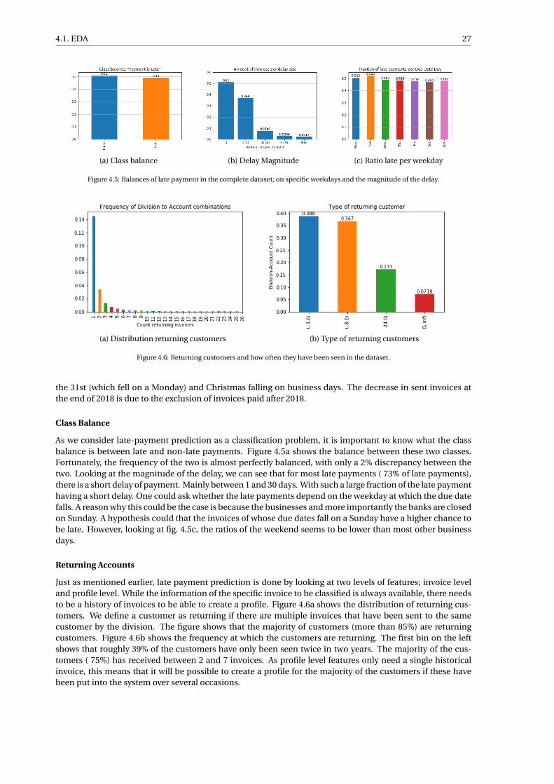
4.1. EDA 27

(a) Class balance (b) Delay Magnitude (c) Ratio late per weekday

Figure 4.5: Balances of late payment in the complete dataset, on specific weekdays and the magnitude of the delay.

(a) Distribution returning customers (b) Type of returning customers

Figure 4.6: Returning customers and how often they have been seen in the dataset.

the 31st (which fell on a Monday) and Christmas falling on business days. The decrease in sent invoices atthe end of 2018 is due to the exclusion of invoices paid after 2018.

Class Balance

As we consider late-payment prediction as a classification problem, it is important to know what the classbalance is between late and non-late payments. Figure 4.5a shows the balance between these two classes.Fortunately, the frequency of the two is almost perfectly balanced, with only a 2% discrepancy between thetwo. Looking at the magnitude of the delay, we can see that for most late payments ( 73% of late payments),there is a short delay of payment. Mainly between 1 and 30 days. With such a large fraction of the late paymenthaving a short delay. One could ask whether the late payments depend on the weekday at which the due datefalls. A reason why this could be the case is because the businesses and more importantly the banks are closedon Sunday. A hypothesis could that the invoices of whose due dates fall on a Sunday have a higher chance tobe late. However, looking at fig. 4.5c, the ratios of the weekend seems to be lower than most other businessdays.

Returning Accounts

Just as mentioned earlier, late payment prediction is done by looking at two levels of features; invoice leveland profile level. While the information of the specific invoice to be classified is always available, there needsto be a history of invoices to be able to create a profile. Figure 4.6a shows the distribution of returning cus-tomers. We define a customer as returning if there are multiple invoices that have been sent to the samecustomer by the division. The figure shows that the majority of customers (more than 85%) are returningcustomers. Figure 4.6b shows the frequency at which the customers are returning. The first bin on the leftshows that roughly 39% of the customers have only been seen twice in two years. The majority of the cus-tomers ( 75%) has received between 2 and 7 invoices. As profile level features only need a single historicalinvoice, this means that it will be possible to create a profile for the majority of the customers if these havebeen put into the system over several occasions.

Chapter 5

Method

In this chapter, we will look into the different experiments surrounding the problem of late payment pre-diction. In previous chapters we have discussed how invoicing is registered in the system and the generalbehaviors around the topic. In combination with the resolved entities, we now have a constructed network ofDutch SMEs that results from it. In this chapter, we will discuss the method for late payment prediction andthe corresponding experiments.

5.1 Overview of late payment experiments

The goal of the experiments is to validate assumptions and to answer the defined sub-questions. The first setof experiments will show how the addition of a single group of custom-crafted features impacts the perfor-mance of the model. Following this, we will show how these features impact the payment prediction on theirown, and in combination with predefined baseline features.

Experiment 1: Node scope profile features (SQ3) . Comparing the cases discussed in the literature, ourdataset contains invoices between a large number of companies. To see whether global information is bene-fiting the prediction of late-payment, we first bring the baseline features to the node level. Meaning that welook at all invoices associated with the sender and receiver of the invoice we are trying to predict.

Experiment 2: Impact of windowing features In this experiment, we look at whether it is beneficial to onlyconsider the most recent invoices. All previous features will be windowed to different human seasonal timeframes. For example windowing on 1-month, 3-month, 6-month, and 12-month basis. The intuition behindthis experiment is that companies and the people responsible for their payments change over time. Recenttimely payments should outweigh the late-payment made years ago and vice-versa.

Experiment 3: Temporal features The goal of the third experiment is to see whether time-related features canimprove the predictions of our models. For this experiment we specifically look at the time-frame betweendifferent payments and how this time-frame changes over the period of time. We will look specifically at thefollowing features:

• gradient of delay at last step

• variance of delay

• time between last late payment

• mean time between late payments

• inverse temporal link weight

Experiment 4: Neighborhood scope features (SQ3) The goal of this experiment is to explore whether per-formance of the models can be improved by introducing information that is available from 1-hop neighbors.More specifically we look at the neighbors of the source node. The features are calculated by gathering theinvoices that are sent by all 1-hop neighbors. Similar to the first experiment, node level features are calculated

29

30 5. Method

Figure 5.1: Overview of experiments and type of the generated feature sets.

using the baseline features. The average of these features create the neighborhood profile feature set.

Experiment 5: Business graph embedding (SQ2, SQ3) To be able to answer SQ3, we look into different possi-ble graph constructions. The business graph only contains the information of which companies do businesswith each other. In terms of the system, two companies do business with each other if one of them has addedthe other as an account. In this experiment the set of features will be extended with latent embeddings ofthe nodes. This will be done with methods such as Node2Vec. However, this method highly depends on theconstructed graph. A part of this experiment (and the following ones) will show how the predictions are im-pacted by the constructed graph of the company invoices.

Experiment 6: Embedding of invoice graphs (SQ2, SQ3) In this experiment we will look how the graph ofcompanies can be constructed using different available information such as accounts and invoices. With thisexperiment we will answer the sub-question of how the graph should be constructed to be able to benefitfrom extracted graph features. Some of the following graph structured will be tested:

• Static graph of companies built from accounts of the divisions. This graph does not any link weights.

• Two static graphs each for a single type of payment. One graph consists of links where a single link isa timely payment between two companies, while the other graph has a link if there is a late payment.The link weight represents the amount of

These experiments and the generated features can be split into two different groups. Namely, Handcraftedfeatures and Learned features. Figure 5.1 shows the overview of the experiments and to which type of featuresthey belong to.

5.2 Featuring

For the baseline the focus will be on the next features: Amount, Payment Term, # paid invoices, # late in-voices, ratio between paid and late invoices, sum of the amount from paid invoices, sum of the amount fromlate invoices, mean delay for all invoices, # of outstanding invoices, average amount of outstanding invoiceamounts, and sum of outstanding invoice amounts. The features have been chosen because this set coversthe majority of the features shown in table 5.1. The baseline features can be splits into the following twogroups:

• Invoice Level features: consist of information that is present on the invoice. Namely the Amount andPayment term of the invoice. This information is always present.

• Profile level features: consist of aggregate information from previous invoices. These features are notavailable if there have not been any invoices sent from the seller to the buyer.

5.2. Featuring 31

PaperFeature Zeng [36] Kim [19] Cheong [8] P Hu [15] W Hu [16]amount x x x x xpayment_term x x xnumber_of_paid_invoices x x x xnumber_of_late_payments x x x xratio_paid_late x x xsum_paid x x x xsum_paid_late x x x xratio_sum_paid_late x x xmean_delay x x xaverage_amount xoutstanding xaverage_amount_outstanding xoutstanding_sum_amount xaccount_manager x xbilling_cylce xintervention_count xdemographic xproducts_used x x

Table 5.1: Table showing which features have been used by different methods. Crossed cell "x" shows that the feature has been used,empty cell shows that the feature was not used.

Profile level features can sometimes be tricky to calculate. As previously discussed, there is a discrepancybetween the current state of invoices and what is visible in the bookkeeping system. This is because theuser does not have to enter both at the same time or within any time period for that matter. What oftenhappens is that there is a significant delay between an invoice being sent or paid and when it is put into thesystem. Analysis of the data shows, that the median time between the invoice date and the date at which theinvoice has been put into the system is 55 days. Looking at payment, the delay is even larger. The mediandelay between an actual payment and when the payment is put into the system is 80 days. An explanationfor this could be that as there are many invoices being sent and received, it is often more efficient for theadministrator to register/import the invoices in bulk every period of time. This period can be weekly, monthlyor even quarterly or yearly. With current median delay, the latter seems to be more common. Nevertheless,the method of administration is company dependent. With a large number of different companies in thesystem, there is a high amount variety in behavior across the invoices in the dataset. This makes it hard topredict when a division is missing a payment. It is uncertain whether the invoice is unpaid or just has notbeen registered yet. For this same reason, it is not possible to assume that an invoice is past due when thedeadline has been past and no payment has not been seen yet. That is why the invoices that do not have aregistered payment are excluded from the dataset.

But besides the missing payments, the delay that is present in most of the data causes problem in thequality of the data too. Figure 5.2 shows how featuring is done with an expanding window. This comes downto going over every invoice in the order that is was supposedly received by the customer, and creating theprofile feature by looking at all previous invoices. As there is no history for the first invoice in the sequence,the features cannot be created for that specific invoice. This is also known as a cold start problem. However,because of the delay in the system, the cold start is prolonged until the invoice and the corresponding pay-ment is put into the system. In a median case, this will be almost 3 months of no data. To be able create ageneric model the training data needs to represent the actual situation at which its is going to be used. Fea-turing is not a problem for it is done at the latest timestep. This is because the most recent snapshot showsall available data by definition. But during modeling, when looking at historical data, only the data should bekept that is available at the point in time at which the invoice is created. And thus during training there is anextra step which filters out all unavailable invoices at each rolling iteration.

32 5. Method

Figure 5.2: Visualization of an expanding window featuring approach. The example shows the calculation of the late-payment ratiofeature. A rolling function iterates over the sequence of invoices (late in red, non-late in blue) for every invoice, every preceding

available invoices are taken and passed to the feature functions.

Figure 5.3: Pipeline from the data source to the prediction of late payments.

5.2.1 Modeling

Once the features are created they can be used to train a model for our problem. To do this we use modelsfrom the most popular machine learning library Sci-Kit Learn [28]. From this library, the Random Forest,Multi-Layered Perceptron and Decision Tree classifiers are used. Additionally, we use LightGBM [18], whichis currently a popular and fast implementation of the Gradient Boosted Decision Tree and Random Forest.Once the models have been chosen, the next steps are taken to create a model that is as generic as possible:

• Random Seed: at the beginning of every run a random seed is set to guarantee reproducibility. Not onlyfor the models but also for the preprocessing steps. In all cases, the random seed is set to 0.

• Dataset consistency: Every experiment has its own method of feature engineering. To make sure thatthe results are comparable across the experiments, the same set of invoices is used over all experimentsunless specified. To keep the dataset consist in among all experiments, the invoices for which featurescould not be generated are padded.

• Dataset split: the complete dataset is split into a training and test set. The training data is roughly 80%,while the test set consists of the remaining 20%. The test set consists of the most recent invoices.

• Balancing: Before the training is done, the dataset is first balanced. This is done by simply oversam-pling the class that is less frequent in the dataset without creating any synthetic samples. This createsduplicate records in the dataset but balances the classes to the same frequency. To make sure that no

5.2. Featuring 33

Figure 5.4: Example of bayesian optimization using the skopt package as described in [24] on the Random Forest Classifier. The x-axisshows the progression in time. The red line shows the trend of the performance.

samples from the test set leak into the training set and as general good practice, the balancing is onlyperformed on the training set of the data.

• Shuffle: the training set is shuffled to make sure that the score of the model does not depend on theordering of the data. This is done because the features are made with an expanding window, the in-voices that are at the end of the dataset have features made from a larger history than the ones at thebeginning. When taking a validation set from the end, the features from this segment are richer thanthe training set. To avoid this, the dataset is shuffled. The test set is unaltered and consists of

• Cross-validation: To reduce the chance of overfitting on the training set, during the training we applyK-Fold cross-validation. During cross-validation, the training set is first split into k folds. One by one,a single fold is chosen and used as a validation set. The remaining folds are used to train the model.At the end of all runs, the scores are gathered from measuring the performance on the test set. In allexperiments, k is set to 5 unless specified otherwise.

• Parameter optimization: as is well known, most machine learning model performances depend on howwell the parameters are optimized for the problem. The input features are different between runs andthus there is no single set of parameters that is optimal in all cases. To make sure that the parametersare separately optimized in combination with the input of the model, parameter optimization is part ofthe pipeline for every run. To do this we use Bayesian Optimization as described in [24]. The methodsearches for more optimal parameters within a predefined parameter space. An example of the processcan be seen in fig. 5.4.

The complete pipeline from the data source to validation can be seen in fig. 5.3 and highlights the dis-cussed steps on a higher level.

5.2.2 Evaluation

To be able to draw conclusions from the proposed experiments there are several methods we use to evaluatethe results. The problem of late payment is defined as This is done by comparing the results of the experi-ments to the proposed baseline (table 2.1, table 2.2) using the Accuracy and Receiver Operating Characteris-tic curve (ROC curve) Area-Under-the-Curve (AUC) metrics. These two metrics are also used in the surveyedlate payment prediction methods. While Accuracy is generally the most popular method of evaluation, AUCshows the quality of the model under different discrimination thresholds. More on AUC can be found in [11].Additionally, in some cases we provide the F1-score of the model. The F1-score considers the recall and theprecision of the predictions.

r ecal l = T P

T P +F N

34 5. Method

RandomForest MLP DecisionTree LGBMAccuracy 0.81558 0.77433 0.77765 0.80442F1 0.83108 0.78749 0.80154 0.81923Recall 0.80734 0.74408 0.80385 0.78866ROC AUC 0.81674 0.77861 0.77418 0.80665

Table 5.2: Performance of Random Forest, Mulit-Layered Perceptron, Decision Tree and LightGBM

Figure 5.5: Feature importance of the Random Forest model on the baseline features

pr eci si on = T P

T P +F P

Recall is the fraction of positive sample (True positives or TP) that are successfully found (TP + False Negativesor FN). The precision of the predictions is similar, but calculates the fraction of the successfully found positivesamples from all positively labeled predictions (TP + False Positives or FP).

F1 = 2 · pr eci si on · r ecal l

pr eci si on + r ecal l

5.3 Baseline

As previously mentioned in chapter 5, to be able to show that the proposed method improves the currentlyavailable methods of late-payment prediction, the results need to be compared to a baseline. This base-line model is constructed from the papers available on the topic of late-payments prediction. Table 2.1 andTable 2.2 show an overview of the used features and models from the literature. In the next section, theseresources are used to construct a baseline.

5.3.1 Results

Table 5.2 shows the performance of several classifiers that have been gathered from the overview of most usedmodelstable 2.2. The Random Forest classifier gives the best results in terms of accuracy, F1 and AUC. Inter-estingly, The LightGBM model is underperforming compared to the RF model. To get a better understandingof the impact of the features, we can look at the feature importance from the trained models. Figure 5.5 showthe feature importance of the RF model. The two most important features seem to be ’Ratio Paid Late’ and’Ratio Sum Paid Late’. These represent the ratio of invoices paid late, and the ratio of the summed amount thatwas late, respectively. In cases where there is a low variance in payment amounts between the invoices, thesetwo numbers should be almost equal. Other features seem to have similar importance to each other, exceptfor the Payment Term feature. To further analyze this, a heatmap is created showing the Pearson correlationbetween the features. This can be seen in Figure 5.6. Similar finding can be seen in the correlation between

5.3. Baseline 35

Figure 5.6: Heatmap showing the correlations between all baseline features.

Payment Term and the target variable, "IsLate". A more interesting find is that almost no feature correlateswith strongly one another. The exception here is "Number of late payments" and "Number of paid invoices".Because of this strong correlation, it can be beneficial to remove this feature from the set as there is a littleamount of information added by leaving the feature in at the cost of run-time.

Chapter 6

Experiments

In this chapter we will discuss the experiments and the methods that have been introduced in chapter 5. Thechapter is split into two segments. The first segment will look into the experimentation of custom features.These are features that have been handcrafted by looking into different scopes for the baseline features or areintroduced as new features altogether. The second segment of the chapter looks into learned features usinggraph embedding.

6.1 Custom features

In this section we will look how the custom handmade features perform to the baseline shown above. Withthese experiments the goal is primarily to test the quality of other custom features other than the ones thatwere shown in the literature. Additionally, these experiments should help us in answering SQ3, namelywhether any additional information from the network improves the performance of our predictions. Thisis done step by step by iteratively increasing the scope of features. To be able to build a graph of that encodesinvoices, a segment of the dataset

6.1.1 Experiment 1: Node level profiling

In this experiment we investigate the effects of raising the baseline features to the scale of the node, to seewhether it improves the accuracy of the model. In the baseline model all features were based on the historybetween the sender of the invoices and its receiver. However, over the duration the two parties are also in-volved with invoices from and to other companies. These transactions could possibly give insight about thebehavior of the two parties by leveraging data of other administrations.For the featuring we introduce two new sets of features. Baseline features calculated on all outgoing invoicesfrom the source entity, and all incoming invoices coming into the target entity. The choice was made toinclude these two sets, and not for example all outgoing invoices of the target entity, is because divisions aremissing this type of data. Purely because the majority of the divisions in the dataset, has not sent any invoicesto another division. However, to avoid any overlap in information between this global information and thebaseline, the pairwise invoices between the source and target have been removed.

Results

The results of the experiment can be summarized by the following tables. The first table shows the results ofthe Random Forest model, which performed best on the baseline, on different segments of the new features.As can be seen in the table, the addition of the incoming and outgoing features next to the existing baselinefeatures increase all measures across the board. The table below shows the other models performed on thiscombination of features.

Similar to the baseline, Random Forest outperforms all models by a margin. Almost for all models the additionof the incoming and outgoing features has increased the performance. However, the MLP model seems tohave trouble with the addition of the dimensionality. With Accuracy slightly higher than 50%, it performsalmost as bad as random guessing.

37

38 6. Experiments

Baseline Incoming Outgoing In + Out Baseline + In + OutAccuracy 0.81558 0.80721 0.75055 0.82508 0.83086F1 0.83108 0.82346 0.77216 0.84048 0.84579Recall 0.80734 0.80011 0.75219 0.82006 0.82541ROC AUC 0.81674 0.80822 0.75032 0.82579 0.83163

Table 6.1: Performance of node level features on a Random Forest model.

RandomForest MLP DecisionTree LGBMAccuracy 0.83086 0.56358 0.79528 0.79104F1 0.84579 0.71995 0.81789 0.80627Recall 0.82541 0.56291 0.81746 0.84138ROC AUC 0.83163 0.66062 0.79211 0.78929

Table 6.2: Performance of multiple classifiers on the combination of incoming invoices of the target node

6.1.2 Experiment 2: Time sensitive customer profiling

In this experiment we look whether it is beneficial to only consider most recent invoices. The features willbe windowed to different human seasonal time frames. For example: windowing on 3-month, 6-month and12-month basis. The intuition behind this experiment is that companies and the people responsible for theirpayments change over time. Recent timely payments should outweigh the late-payment made years agoand vice-versa. The difference between these features and the baseline is that for the baseline completeaggregates are taken for all available data. Because of this, features such as the Sum of Invoice Amounts willhave larger values the more invoices and time are available.

So for this experiment the featuring is done using time windows, instead of all preceding data points.Primarily windows of 3-months, 6-months and 1-year. Because of the way the windowed methods calculatethe features there are often more sparse. For example, when no invoices are sent within the period of thewindow. In order to keep the datasets the same between the experiments and the baseline, the features arepadded with zeroes in cases where the feature cannot be calculated. The following table shows the result ofthe experiment.

As can be seen in table 6.3 limiting invoices to a recent time window does not directly improve the ac-curacy of the model. This could be due to how different divisions are amongst each other. The dataset con-tains roughly 150000 with each their own types of behaviors. Moreover, there is a high variance between theamount of invoices that every division sends. Among these divisions majority only sends several invoices ayear, while others send hundreds. In future steps the static n-day window of time could be replace by a moredynamic method that considers the amount of invoices that are sent by the divisions.

6.1.3 Experiment 3: Alternatives to profile features

In this experiment we look whether new features can be introduced that consider the late payments and thedelay of the payments as a signal. Specifically in this experiment we will look at the following features:

• gradient/slope of delay at last steps

• variance of delay

• time since last late payment

• mean time between late payments

Baseline 90-day window 180-day window 365-day windowAccuracy 0.81558 0.78573 0.80992 0.81541F1 0.83108 0.80335 0.82555 0.83085Recall 0.80734 0.77883 0.80039 0.80674ROC AUC 0.81674 0.78670 0.81126 0.81663

Table 6.3: Results based on several metrics using the Random Forest model

6.1. Custom features 39

Baseline Temporal Baseline + TemporalAccuracy 0.81558 0.77002 0.81489ROC AUC 0.81674 0.76335 0.81575

Table 6.4: Performance of hand crafted temporal features compared to the baseline.

Baseline Neighborhood Baseline + Neighborhood Baseline + In + Out + NeighborhoodAccuracy 0.81558 0.73463 0.82790 0.83265ROC AUC 0.81674 0.73193 0.82533 0.82998

Table 6.5: Performance of neighborhood features on Random Forest model compared to the baseline and previous node level featureexperiment.

• inverse temporal link weight

Compared to the existing features, with these features we look at the delay and the late payments as asignal. With the gradient and variance we try to get more information on the volatility of the target’s payments.For example, if the customer is becoming more lax over time this would be visible in the the gradient of thedelay. The mean time between late payments and the time since the last late payment can could be useful ifthe late payments are done periodically. The inverse temporal link weight is inspired by the Temporal LinkWeight introduced in [37]. The goal of the feature as described in the paper is to assign more weight to eventsthat happened early in the process to account for the possible spreading and snowball-effect. For our usecase we would like to do the opposite, and rather have the weight to be high if the payment were made laterecently and decay the weight over time. This is done using the following formula of Inverse Temporal LinkWeight:

φ(α) =n∑

m=1(

t (m)j k

tmax)α

The event at which there is a late payment is defined by t (m)j k , from node j to node k at timestep m. tmax is

the normalizing factor and is set to the latest possible timestep m. Since we have two years of data, tmax is setto 730. The factor α is set with α> 1 to increase the weight exponentially the more recent it is. The parametercan be used to create similar features but with different settings for alpha. Looking at the other featuresthe calculations more are straightforward. With the gradient, the delay is first smoothed out using a movingaverage. The slope is then taken at the last step. The calculation of the other features is straightforward. Thefollowing table shows these features perform compared to our baseline:

As can be seen from table 6.4, these features do not perform as well as the baseline features. However,these features perform only 5% worse than the baseline, with a very small feature set. The benefits of this isthat the training is quicker and easier to tune as a result. The combination of the baseline and the temporalfeatures does not seem to show any improvements.

6.1.4 Experiment 4: Neighborhood level profiling

The goal of this experiment is to explore whether performance of the models can be improved by introduc-ing information that is available from 1-hop neighbors. More specifically we look at the neighbors of thesource node. This is similar to the node level features in experiment 1. However, now instead of looking atthe invoices neighborhood pays, we look into the invoices that are sent by the neighborhood. The baselinefeatures aggregate the invoices from the neighborhood and generate a single set of features. This should giveinformation about how much money the neighborhood has and how much they are still owed by others.

Table 6.5 shows the performance of these generated features. As can be seen from the table the neigh-borhood features perform well when combined with the baseline feature set. The results from experiment1 showed that node level profiles can improve the performance of the predictions, even when the featuresare made from a similar set of invoices. The neighborhood features on the other hand do not use any of theinvoices that have been used by the other features sets. However, the results from table 6.5 do not show alarge increase in performance when combined with the incoming and outgoing features. Moreover, compar-ing to the results from experiment 1, the increase is marginal. Nonetheless, with the use of the same definedfeatures as in the literature but raising the scope at which they are calculated, we have increased the perfor-mance. The next section will show how this can be done with learned features.

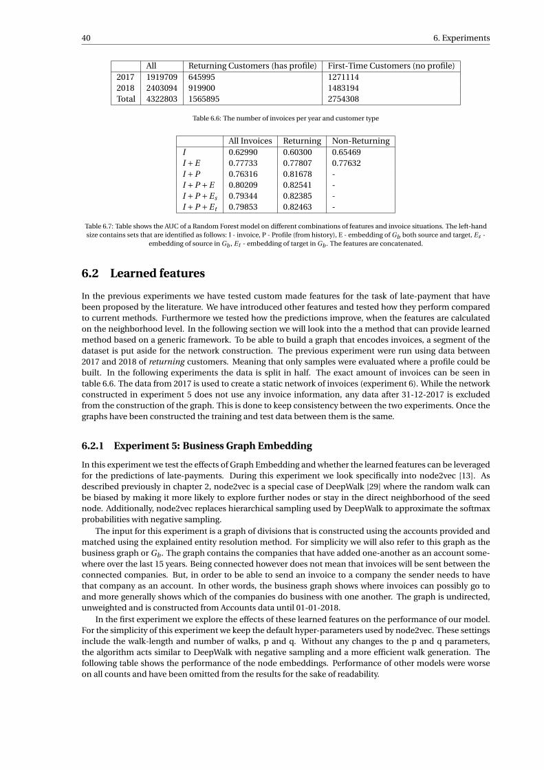
40 6. Experiments

All Returning Customers (has profile) First-Time Customers (no profile)2017 1919709 645995 12711142018 2403094 919900 1483194Total 4322803 1565895 2754308

Table 6.6: The number of invoices per year and customer type

All Invoices Returning Non-ReturningI 0.62990 0.60300 0.65469I +E 0.77733 0.77807 0.77632I +P 0.76316 0.81678 -I +P +E 0.80209 0.82541 -I +P +Es 0.79344 0.82385 -I +P +Et 0.79853 0.82463 -

Table 6.7: Table shows the AUC of a Random Forest model on different combinations of features and invoice situations. The left-handsize contains sets that are identified as follows: I - invoice, P - Profile (from history), E - embedding of Gb both source and target, Es -

embedding of source in Gb , Et - embedding of target in Gb . The features are concatenated.

6.2 Learned features

In the previous experiments we have tested custom made features for the task of late-payment that havebeen proposed by the literature. We have introduced other features and tested how they perform comparedto current methods. Furthermore we tested how the predictions improve, when the features are calculatedon the neighborhood level. In the following section we will look into the a method that can provide learnedmethod based on a generic framework. To be able to build a graph that encodes invoices, a segment of thedataset is put aside for the network construction. The previous experiment were run using data between2017 and 2018 of returning customers. Meaning that only samples were evaluated where a profile could bebuilt. In the following experiments the data is split in half. The exact amount of invoices can be seen intable 6.6. The data from 2017 is used to create a static network of invoices (experiment 6). While the networkconstructed in experiment 5 does not use any invoice information, any data after 31-12-2017 is excludedfrom the construction of the graph. This is done to keep consistency between the two experiments. Once thegraphs have been constructed the training and test data between them is the same.

6.2.1 Experiment 5: Business Graph Embedding

In this experiment we test the effects of Graph Embedding and whether the learned features can be leveragedfor the predictions of late-payments. During this experiment we look specifically into node2vec [13]. Asdescribed previously in chapter 2, node2vec is a special case of DeepWalk [29] where the random walk canbe biased by making it more likely to explore further nodes or stay in the direct neighborhood of the seednode. Additionally, node2vec replaces hierarchical sampling used by DeepWalk to approximate the softmaxprobabilities with negative sampling.

The input for this experiment is a graph of divisions that is constructed using the accounts provided andmatched using the explained entity resolution method. For simplicity we will also refer to this graph as thebusiness graph or Gb . The graph contains the companies that have added one-another as an account some-where over the last 15 years. Being connected however does not mean that invoices will be sent between theconnected companies. But, in order to be able to send an invoice to a company the sender needs to havethat company as an account. In other words, the business graph shows where invoices can possibly go toand more generally shows which of the companies do business with one another. The graph is undirected,unweighted and is constructed from Accounts data until 01-01-2018.

In the first experiment we explore the effects of these learned features on the performance of our model.For the simplicity of this experiment we keep the default hyper-parameters used by node2vec. These settingsinclude the walk-length and number of walks, p and q. Without any changes to the p and q parameters,the algorithm acts similar to DeepWalk with negative sampling and a more efficient walk generation. Thefollowing table shows the performance of the node embeddings. Performance of other models were worseon all counts and have been omitted from the results for the sake of readability.

6.2. Learned features 41

Figure 6.1: t-SNE clustering of the embeddings made with node2vec

The table shows results for the follow feature sets, the baseline, baseline with the embedded features ofthe source node concatenated, same as the previous but the embeddings of the target node are also concate-nated. For the final setup the node embedding features have been reduce in dimensionality using PCA. UsingPCA the dimensionality of the embedding is reduced from 128 to 10. As can be seen from the table, in allcases where the node features have been added to the existing baseline feature set, the prediction improved.The biggest improvement is when the embedding of both nodes is added. Although, individually it seemsthat information about the target is slightly more important than source embedding. The most interestingresults are regarding the performance of the embeddings when the profile of a companies is not available.There is a major increase in performance compared to predicting the late payment based on only invoice in-formation. The invoice information only consists of the Amount that needs to be paid and the correspondingpayment term. This is a major benefit to a late payment framework. From the surveyed literature, none wereable to make predictions when there was no historical data. The use of these features opens the possibilityto classify invoices where no other invoices are present in the history. In other words these types of featurescan help solve the cold start problem by providing context features of the companies involved. With such alarge fraction of the dataset suffering from the cold start problem, this method provides a large improvementcompared to the methods gathered from the literature.

Ofcourse the increase in utility and performance does not come entirely free. A Problem with node em-beddings in general is that it cannot be updated when new data becomes available. This can be a problemwith using graph embedding for classification. The runtime of the embedding algorithm scales primarilywith the amount of edges in the graph. While the featuring of the profile features can be done in about 20minutes, the embedding of the accounts graph takes almost 12 hours to run. While this is not a problem inthe grand scheme of things, it is not possible to recalculate the embedding every time a new connection ismade. This is a known problem that many graph embedding methods struggle with. A compromise could bethat the embedding is calculated once a day for the next day or even once a week or once a month dependingon the availability of the resources and the size of the graph. A more dynamic method of using the embeddedfeatures is tested in further experiments.

As can be seen from the table, the learned features gives a better prediction in a situation where onlyinvoice information is present. The combination of the invoice features and the learned features further in-

42 6. Experiments

Figure 6.2: Scatter plot (left) and heatmap (right) of the t-SNE embedding showing the relation to the position of a node and itspercentage of received late payments.

creases the accuracy. Interestingly, the learned features are not dependent on time or the previous invoicesbetween the companies. Moreover, none of the invoice information is embedded in them. But rather thefeatures are supposed to represent the nodes in a latent space. Whether these latent features could be inter-preted and correlated to an aspects of the company is still an open research problem.

Work from Bruss et al. [5] shows different ways of how these features are incorporated into their predic-tion. The paper discusses two different methods, namely directly concatenating the feature set or training aseparate classifier that and passing the predictions as a feature to the existing classifier. The first method hasbeen described above. However, while being the superior method in the paper discussed by Bruss, similarimprovements were not seen during experimentation. Moreover the general results of this method show areduction in performance across the board from 3% to 4%. Due to its performance and overall readability ofthe chapter, the results of the stacking have been omitted.

To understand why there is such an increase in performance we explore the embedding by visualising itusing t-SNE. The main benefit of t-SNE is that it is a great method for visualizing high dimensional data intoreadable 2-dimensional clusters. More on t-SNE can be found in [25]. Figure 6.1 shows the created repre-sentation embedded to a 2-dimensional space using t-SNE. The sector information of a few largest sectors islabeled after the dimensional reduction is applied, to show possible similarity between companies. The plotclearly shows clustering and segmentation of nodes that share the same sector. It is important to note thatthe sector information has not been used during any of the preprocessing or embedding of the networks. Ad-ditionally, this shows that the graph generated using entity resolution is well structured and carries valuableinformation about the supply chain between the SMEs in the graph.

fig. 6.2 shows the relation between the position of a node and its percentage of received late payments.The scatterplot shows the exact location and ratio of late payment of a node, but it is prone to overlapping.The heatmap on the other hand, divides the plane into a grid and calculates it per cell. However, this causesextreme values in cells where there are not enough nodes. Disregarding this, both visualizations do not showthat the position of the node corresponds to its likeliness to pay late. Finally, we can look whether the combi-nation of certain sector pairs is more likely to have late payments. This can be seen in fig. 6.3. The hue of thecells shows the ratio of late payment while the annotated number shows the actual amount of invoices in thatcell. While there are no clear heavy hitters, sectors such as the Industrial sector receive a fairly high amountof late payments from the Distribution of water and waste sector.

6.2.2 Experiment 6: Invoice Graph Embedding

In the previous experiment we have shown learned features which were gathered using node embeddings onthe business graph. This graph only contained information about which companies do business with eachother. This graph did not contain any further information about the invoices sent between nodes. However,creating a network that models the invoices between companies is not a trivial task, especially as node em-bedding methods are only limited to (un)directed and (un)weighted graphs. With invoice being able to beeither late or on-time, we cannot model the events with a single network unless the edges are typed. Un-fortunately, this is not supported by the node2vec architecture unless some workaround is applied. To still


Figure 6.3: Heatmap shows the interaction between the sector of the source node and the target node. Annotated values show the countof invoices with this sector combination, where as the hue describes the ratio of invoices that have been paid late.

44 6. Experiments

All Invoices (Business Graph) All Invoices (Invoice Graphs)I 0.62990 0.62990I +E 0.77732 0.77919I +P 0.76316 0.76316I +P +E 0.80209 0.80020I +P +Eneg - 0.79701I +P +Epos - 0.79800I +P +Es 0.79344 0.78830I +P +Et 0.79853 0.79676

Table 6.8: Comparison of business graph embedding versus embedding of the invoice graph measuring AUC. The left-hand sizecontains sets that are identified as follows: I - invoice, P - Profile (from history), E - embedding of both source and target, Es -

embedding of source, Et - embedding of target, Epos - embedding of source and target from the late invoice graph., Eneg - embeddingof source and target from the non-late invoice graph. The features are concatenated.

Figure 6.4: Choice of binary operators for learning edge features. The definitions correspond to the i th component of g (u; v).

be able to use node2vec for the node embedding the invoices are split over two separate graphs. One ofthe graphs contains all late invoices while the other contains all invoices that were paid on time. Unlike thebusiness graph, these graphs are directed in the direct of the node that receives the invoice. These edges arealso weighted. This weight represents the count of invoices that have been paid by the receiver(target) to thesender(source). Further exploration shows the quality of the generated features and performance when thenode2vec framework is tuned.

The most simple way of using the generated features is to direct use the latent features as the input to theclassifier. With two graphs, this results into a total of 4 sets of features. The embedding of the source nodefrom both graph, and the same for the target node. However, due to the embedding not always being avail-able, for example because a node has never sent or received late invoice payments, the feature set is paddedto match the input size. Table 6.8 shows the performance of the embedded features compared to the em-bedding of the business graph. This set of features performs very similar to the performance of the businessgraph but at the benefit of faster runtime.

This method decreases the runtime of the algorithm in two different ways:

1. Since invoices can only be sent to existing accounts, the invoice graph is a subset of the business graph.With only a fraction of the accounts receiving invoices, the invoices graph count significantly less edgesthan the business graph.

2. Additionally the two graphs are directional. This reduces the amount of possible paths and reduces thetime needed to calculate the transition probabilities.

Alongside the node2vec frame work, Groover et al. provide several operators that can be used to do classi-fication on edge level. These operators are shown in fig. 6.4. According to the paper, the Hadamard operatoroutperformed raw features and any other operators that were tested. Testing out this operator, we combinethe raw features of the embedded target and source nodes using the Hadamard operator. This is done foreach graph separately. However, the performance of the operator is lower than using raw features as input byroughly 3% across the board and has therefore been omitted from the report.

6.2.3 Split graph tuning

Looking at the previous experiments, we saw that the introduction of dimensionality reduction improved theperformance of the model. This suggests that the default embedding dimensionality of 128, is possibly too


Figure 6.5: Figure showing the performance of the model per different embedding sizes.

large for the graph and could possible be reduced. Looking at work done by Bruss et al. [5], the embeddingsize of the their network was the most optimal around size 10. To investigate the effect of the dimensionalitysize, we create several embedding at different embedding sizes. This can be seen in fig. 6.5.

The different embeddings show that the more optimal embedding sizes are much lower than the defaultembedding size of 128 set by node2vec. The embedding size is set for both graphs at the same time. Theperformance is measured The embedding size that gives the best performance seems to be 12 from the set ofparameters that has been tried out. This is consistent with all performed metrics.The general performance from the node embedding experiments have been very promising. However node2vecand graph embedding methods can really give different results depending on the tuning of the hyper-parameters.So in the following steps we will look into the performance differences when the embedding method is tuned.Specifically, we will look into the walk length, number of walks, p and q. Where the latter two bias the randomwalk probability.

The tuning of these parameters is done using Grid Search. This comes down to exhaustively trying outall parameter given combinations. With 4 hyperparameters and 5 settings for each parameter, totals to 625trials. The chosen search space is similar to the one discussed in [13] with p and q values between 0.25 and2.0. Figure 6.6 shows the mean results of the tuned parameters. As can be seen from the figures the meandifference in AUC varies only slightly between the trials. This can be seen throughout the measurement ofthe trials.

46 6. Experiments

Figure 6.6: Mean results of tuned node2vec parameters.

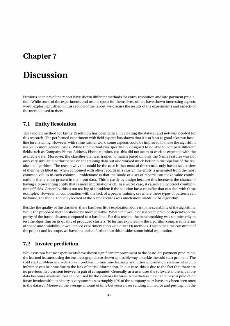
Chapter 7

Discussion

Previous chapters of the report have shown different methods for entity resolution and late payment predic-tion. While some of the experiments and results speak for themselves, others have shown interesting aspectsworth exploring further. In this section of the report, we discuss the results of the experiments and aspects ofthe method used in them.


The tailored method for Entity Resolution has been critical in creating the dataset and network needed forthis research. The performed experiment with field experts has shown that it is at least as good a known base-line for matching. However, with some further work, some aspects could be improved to make the algorithmusable in more general cases. While the method was specifically designed to be able to compare differentfields such as Company Name, Address, Phone number, etc. this did not seem to work as expected with theavailable data. Moreover, the classifier that was trained to match based on only the Name features was notonly very similar in performance on the training data but also worked much better in the pipeline of the res-olution algorithm. The reason why this could be the case is that most of the records only have a select viewof their fields filled in. When combined with other records in a cluster, the entity is generated from the mostcommon values in each column. Problematic is that the mode of a set of records can make value combi-nations that are not present in the input data. This is partly by design because this increases the chance ofhaving a representing entity that is more information-rich. In a worse case, it causes an incorrect combina-tion of fields. Generally, this is not too big of a problem if the solution has a classifier that can deal with theseexamples. However, in combination with the lack of a proper training set where these types of patterns canbe found, the model that only looked at the Name records was much more stable in the algorithm.

Besides the quality of the classifier, there has been little exploration done into the scalability of the algorithm.While the proposed method should be more scalable. Whether it would be usable in practice depends on thepurity of the found clusters compared to a baseline. For this reason, the benchmarking was set primarily totest the algorithm on its quality of produced clusters. To further explore how the algorithm compares in termsof speed and scalability, it would need experimentation with other ER methods. Due to the time constraint ofthe project and its scope, we have not looked further into this besides some initial exploration.

7.2 Invoice prediction

While custom feature experiments have shown significant improvement to the basic late payment prediction,the learned features using the business graph have shown a possible way to tackle the cold start problem. Thecold start problem is a well-known problem in machine learning and other information systems where noinference can be done due to the lack of initial information. In our case, this is due to the fact that there areno previous invoices sent between a pair of companies. Generally, as a user uses the software, more and moredata becomes available that can be used by the system’s features. Nonetheless, having to make a predictionfor an invoice without history is very common as roughly 40% of the company pairs have only been seen oncein the dataset. Moreover, the average amount of time between a user sending an invoice and putting it in the

47

48 7. Discussion

system easily racks up to several months. Because of this, a large segment of the invoices does not have ahistory during inference. In this case, it is possible that only information is available about the invoice itselfand nothing more.

At the same time, there are different features that could potentially help the performance of the predic-tions. For example, when no history is available for transactions between two companies, it is sometimespossible to use the information from the other transactions of the nodes. This information is of course onlyavailable if the nodes have exchanged invoices with other nodes in the network. While we have not exten-sively experimented with extended versions of the baseline. From experience, these methods underperformcompared to the learned node embeddings. Nevertheless, no exhaustive research has been done in exploringnew types of baselines for invoices dealing with the cold start problem. Newfound features could be used incombination with learned node embeddings to improve the performance further.

Interestingly, the results of the business graph experiment show that the embedding of the target nodedoes not provide any improvements to the performance of the model. A reason for why this could be thecase is because the profile is already strictly information about the target. However, this would suggest thatthe addition of the context to the profile does not give any additional information that can be of use to themodel. More generally, the performance of the node embedding on the business graph could possibly bedue to it being the superset of the invoice graph. Additionally, the business graph contains more connectionscompared to the graph of invoices. This due to the fact that not every division sends invoices or has registeredeverything within the period that has been explored during this research.

Thanks to the entity resolution done by the proposed method, we are not only able to solve the cold startproblem but do much more. Since the business connection only has to be done by one side of the relation,we in some cases can make predictions for companies that have not even become a part of the platform yet.Of course, it is important to understand what is allowed with the data and when you are crossing any moralor ethical boundaries. Nonetheless, these examples show the added utility of the proposed methods.

Chapter 8

Conclusion

In this report, we have presented how late-payment prediction can be done through graph features when re-lational data is not available. In the first steps of the project, we have introduced a method that can generatethe needed relational data through recognition of shared connections and matching of entities. In furthersteps, this network of companies has been used to not only improve the existing methods of late paymentprediction but also provide utility in cases where very little information is available.

At the start of the research, a set of questions were defined to guide research and to clarify a general goal of theproject. The main research question was as follows: Can graph features be used to improve the predictionof late invoice payments compared to currently popular methods? With the research completed, we havesufficiently gathered enough information to answer the defined sub-questions.

SQ1: How can a network of SMEs be built from data that is unstandardized, noisy and partial?To create the needed relational dataset a tailored entity resolution algorithm was created. The algorithmshowed that similar records can be found by leveraging the most frequent values in a cluster and move sep-arate records between clusters using a matching classifier. It was shown that the pureness of the createdclusters is similar to the currently best case scenario baseline. Additionally, the algorithm can create clustersfrom incomplete data that is beyond the capabilities of the baseline.

SQ2: How should the data and the graph be structured to be able to extract meaningful features?With one of the following two methods, (1) graph that shows business between companies and, (2) a setupwhere late and non-late payments are constructed separately. The business graph represents the most sim-ple network construction possible and does not contain any invoice information. The embedding of a largegraph can be slow and thus difficult to tune. With the construction of the split invoice graph, the embeddingtime is reduced from 12 hours to 20 minutes. This makes the method much more usable when training timeis an issue. The two methods showed similar results and both improved over the performance of the baseline.

SQ3: Does the addition of graph features improve the prediction of late payments?As can be seen from the results, the addition of the extracted features has improved the performance in sev-eral of the experiments. Besides improving on the baseline, the learned node embeddings give a large amountof utility by unlocking the possibility to predict invoices where invoice history is not available. Meaning it isthe case for both new and returning customers. The visualization of the latent features has shown that entityresolution has been successful in constructing a network that holds vital contextual information.

49

Chapter 9

Future Work

In this section, we will discuss the possible future steps for the described method and implemented frame-work. Some of these features are aspects where we think the research done and the proposed frameworkcould benefit from if looked into. Many of these aspects are direct follow-ups for the research done. However,due to the limited time and scope of this thesis, these aspects were not further investigated.


Throughout the project, a method was developed that successfully was able to apply entity resolution on alarge dataset. Having done this, and having used this method to build a relational graph of Dutch SMEs, hascreated many opportunities. The future work in this segment is not only focused on improving the resolutionalgorithm but also into possible avenues for the created network.

9.1.1 Matching based on context information:

The proposed algorithm provides a method for entity resolution based on the information that is provided inthe accounts of the divisions. From further experimentation and testing with field experts, it became appar-ent that sometimes there was not enough information provided by the records to decide whether they match.However, as these accounts are used for functionalities such as invoicing and other types of transactions, it ispossible to leverage the information that is provided in these transactions as context to improve the resolu-tion. This can be done for example, by recognizing similar templates across invoices or data mining contextfrom descriptions of transactions.

9.1.2 Recognition of private entities:

A major challenge in this data is the separation between private entities and natural persons. This problemarises due to the similarity in naming between the two types of entities. For example, taking the followingtwo names: Albert Heijn and Alfred Heijn. While the two names are very similar in terms of character-levelsimilarity, they represent different types of entities. While Albert Heijn is a large franchise of supermarkets,Albert Heijn is probably a person. This type of ambiguity increases the noise in the data and poses a majorproblem for the quality of the resolved entities. Since the goal of the algorithm is to match the record togetherthat belongs to an entity (private and public) and give a single clean representation of that entity, it is in thebest interest to filter out the natural persons out as part of the algorithm pipeline.

9.1.3 Testing on public datasets:

While the method was specifically made for the problem for Exact’s dataset, it is not completely limited interms of the dataset. Due to how the algorithm works, it should be usable on other datasets once a set ofcolumns has been chosen for grouping.

51

52 9. Future Work

9.2 Late-Payment prediction

While there have been many different features that have been tried and experimented with, we have onlyscratched the surface of what is possible. There are still many types of features and methods that could beused to improve the performance of the models and give more insight into how these businesses interact witheach other.

9.2.1 Modeling of cashflow and node interactions

While the goal of this research was to see whether existing late payment prediction methods could be im-proved using network information. The overarching reason for modeling invoices is due to it being used toestimate a companies cashflow. With this project serving as a proof of concept for the usefulness of the net-work, it would be interesting to see whether it could be used to model the flow of cash from one business toanother. With a large sample of the Dutch SMEs, such research could be used to model the Dutch economy tosome extent. Besides cash flow, it would be interesting to see whether other interactions between companiescould be modeled. For example, the flow of goods, change in KPI’s or bankruptcy status.

9.2.2 GNN models

One method that could perform very well on the data is the set of models that fall under Graph Neural Net-works. The majority of these methods make use of the Graph Convolutional layer that learns features fromthe proximity of each node. A major problem with this approach is that it is much slower and scales muchworse than the methods that have been applied in this research. Nonetheless, GNNs also knows as GeometricDeep Learning is currently a very active field that has many different fields it is applied in. However, as writingthis report, I have not seen any GNN applications in the scope of financial networks or payment predictions.Due to the scalability, the complexity of the GNN architectures and the scope of the project, GNNs were leftfor future steps.

Appendix A

Experiment protocol: Investigating thesubjective quality of generated entities.

A.1 Motivation

Entity Resolution (ER) describes the problem of finding unique entities in a single or among multiple sourcesof records. The later is more commonly known as record linkage if the goal of the method is to enrich adatabase with external information. Record linkage methods are generally measured by the precision andrecall of the classification if ground truth is available. However these methods of validation can be problem-atic [14]. Moreover, whether the mapping of entities is good enough for the task at hand, is task dependentand somewhat subjective. The baseline method that will be compared against are clusters made by groupingthe records on the Chamber Of Commerce number, also known as Kamer van Koophandel (KvK) number. Tounderstand whether the method provides a better representation compared to the current standard or othertype of baseline, the methods should be compared in a subjective test. Within this test records from a singlecluster will be evaluated by a domain expert. This will show the quality of the generated cluster, and whetherit brings an improvement compared to the current baseline.

A.2 Research Questions

The goal of the experiment is to find out how the proposed clustering methods perform in when evaluatedby domain experts. Moreover, we are trying to find whether the proposed method outperforms the baselineduring the evaluation.

• How pure are the clusters made with KvK and the proposed method?

• Does the proposed method provide better clusters compared than the current baseline method?

A.3 Independent Variables / Setup

The independent variable in this experiment is the source algorithm which has grouped the records shownto the expert. To make a sure that the clusters are comparable to each other, we will include records of thesame entity. Additionally, for both methods, the same data will be used to create the clusters. The question-naires consists of 18 multiple choice questions, one question for each of the following: 2 algorithms and per(baseline, proposed) algorithm, 4 large, 4 medium and 4 small clusters. The cluster sizes are classified asfollows:

• large: cluster size between 10000 and 5000

• medium: cluster size between 1000 and 500

• small: cluster size between 100 and 50

53

54 A. Experiment protocol: Investigating the subjective quality of generated entities.

Every question will show 10 different records, which gives a sample size of 120 per algorithm/version/personcombination. Each records has a checkbox next to it. The user is able to check any of the records that he/shefinds to be clustered incorrectly. We expect that a single question will take roughly 30 seconds to complete.With 24 questions, it will take a user about 12 minutes to complete the task. For the experiment we perform awithin group comparison, giving us evaluations of several clusters. To cover a larger set of clusters, the ques-tionnaire will be generated using random companies every single time. Every version will have a different setof companies. This is to cover as much clusters from the methods as possible while keeping the questionnaireshort and with some variation in terms of entities. We hope to have at least 3 people per version, that is atleast 9 human subjects in total.

For every subject, we will create an excel sheet that contains the questionnaire in one of the three ver-sions. The subjects will not have any overlapping clusters. The human subjects will be asked to evaluate thequestions without using any external resources. To make sure that there is no learning or recency effects,the order of the questions will be randomized. To have as least noise as possible in the produced labels, thehuman subject should be a field expert.

A.4 Brand level vs Franchise level

Entities exist on different levels of branding. To be able to distinguish companies from the brands, the focuswill be on comparing records on individual company level. For example, different McDonald’s restaurantscould be grouped on a brand level, encapsulating all franchised restaurants. However, for further use casesof the algorithm it is important to distinguish between different real-world entities. The problem with tryingto make a distinction between a brand level and franchise level entity, is that there often was not enoughinformation to make that choice. The majority of accounts have missing values, which makes the sample alot more uncertain. Because of this, the experts will specifically be asked to distinguish the companies onfranchise level and not on brand level if possible.

A.5 Validation

For the validation we will look at the following aspects of the produced labels:

• Number of defects per human subject.

• Number of defects per algorithm.

To show the significance of these measurements, a Chi-square test will be performed on the results. The con-clusion of the experiment will conclude whether or not the proposed ER algorithm outperforms the baseline,and will show how pure both methods are when evaluated by field experts.

Appendix B

Experiment Briefing

Thank you for helping us test the quality of the account matching algorithm. The goal of the matching al-gorithm is to group accounts together that belong to a single entity. We define an entity as a brand-levelcompany, organization or person. The match is made by cross-referencing the given information to other"similar" accounts.

To validate the quality of the algorithm, we would like to ask you help us find mismatched accounts. To dothis, we have created a list of questions. Every question will contain a set of accounts sampled from a singlecluster. These clusters are either made by matching accounts on KvK or by the proposed method. As part ofthe questions we ask you to checkmark the records you think do not belong with the rest of the accounts. Ifnone of the accounts belong together, you can mark all of the records.

The questions are set up as follows:

• Every question will contain a sample of 10 accounts.

• Every account will show you basic information such as Name, Address, Postalcode, Emailaddress of thecorrespondent, Website and Phonenumber. However, not all information is always provided.

• The questions are generated randomly and were not handpicked.

• For every entity, there will be a question made by each of the methods. Naturally, you will not know bywhich algorithm the records were grouped.

• This also means that there will be multiple questions about the same company.

• The comparison can seem difficult, but you can go back to previous questions.

• The questions don’t necessarily have defect records. There are no wrong or right answers.

Further notes:

• Please read through all the information in a single question before checkmarking any of the records.

• If you are unsure about your choice, it is possible to use external sources to help you (e.g. Google).

• Some clusters contain accounts that are almost 15 years old.

• In case the company changed its name, both new and old names will be present in the cluster.

55

Bibliography

[1] 3 top data challenges and how firms solved them. URL https://www.ibmbigdatahub.com/blog/3-top-data-challenges-and-how-firms-solved-them.

[2] Microsoft dynamics 365 late payment prediction. https://appsource.microsoft.com/en-us/product/dynamics-365-business-central/PUBID.microsoftdynsmb%7CAID.late-payment-prediction%7CPAPPID.3d5b2137-efeb-4014-8489-41d37f8fd4c3?tab=Overview. Accessed: 2019-06-02.

[3] Business content: Payment predictions: Sap analytics cloud, Feb 2019. URL https://www.sapanalytics.cloud/resources-business-content-payment-predictions/.

[4] Joan Bruna, Wojciech Zaremba, Arthur Szlam, and Yann LeCun. Spectral networks and locally connectednetworks on graphs. arXiv preprint arXiv:1312.6203, 2013.

[5] C Bayan Bruss, Anish Khazane, Jonathan Rider, Richard Serpe, Antonia Gogoglou, and Keegan E Hines.Deeptrax: Embedding graphs of financial transactions. arXiv preprint arXiv:1907.07225, 2019.

[6] Hongyun Cai, Vincent W Zheng, and Kevin Chen-Chuan Chang. A comprehensive survey of graph em-bedding: Problems, techniques, and applications. IEEE Transactions on Knowledge and Data Engineer-ing, 30(9):1616–1637, 2018.

[7] Haochen Chen, Bryan Perozzi, Rami Al-Rfou, and Steven Skiena. A tutorial on network embeddings.arXiv preprint arXiv:1808.02590, 2018.

[8] Michelle LF Cheong and Wen SHI. Customer level predictive modeling for accounts receivable to reduceintervention actions. -, 2018.

[9] Adam Cohen. Fuzzywuzzy. URL https://chairnerd.seatgeek.com/fuzzywuzzy-fuzzy-string-matching-in-python/.

[10] Don Coppersmith and Shmuel Winograd. Matrix multiplication via arithmetic progressions. Journal ofsymbolic computation, 9(3):251–280, 1990.

[11] Tom Fawcett. An introduction to roc analysis. Pattern recognition letters, 27(8):861–874, 2006.

[12] Justin Gilmer, Samuel S Schoenholz, Patrick F Riley, Oriol Vinyals, and George E Dahl. Neural mes-sage passing for quantum chemistry. In Proceedings of the 34th International Conference on MachineLearning-Volume 70, pages 1263–1272. JMLR. org, 2017.

[13] Aditya Grover and Jure Leskovec. node2vec: Scalable feature learning for networks. In Proceedings of the22nd ACM SIGKDD international conference on Knowledge discovery and data mining, pages 855–864.ACM, 2016.

[14] David Hand and Peter Christen. A note on using the f-measure for evaluating record linkage algorithms.Statistics and Computing, 28(3):539–547, 2018.

[15] Peiguang Hu. Predicting and improving invoice-to-cash collection through machine learning. PhD thesis,Massachusetts Institute of Technology, 2015.

[16] Weikun Hu. Overdue invoice forecasting and data mining. PhD thesis, Massachusetts Institute of Tech-nology, 2016.

57

https://www.ibmbigdatahub.com/blog/3-top-data-challenges-and-how-firms-solved-them

https://www.ibmbigdatahub.com/blog/3-top-data-challenges-and-how-firms-solved-them

https://appsource.microsoft.com/en-us/product/dynamics-365-business-central/PUBID.microsoftdynsmb%7CAID.late-payment-prediction%7CPAPPID.3d5b2137-efeb-4014-8489-41d37f8fd4c3?tab=Overview




https://www.sapanalytics.cloud/resources-business-content-payment-predictions/

https://www.sapanalytics.cloud/resources-business-content-payment-predictions/

https://chairnerd.seatgeek.com/fuzzywuzzy-fuzzy-string-matching-in-python/

https://chairnerd.seatgeek.com/fuzzywuzzy-fuzzy-string-matching-in-python/

58 Bibliography

[17] Richard HG Jackson and Anthony Wood. The performance of insolvency prediction and credit risk mod-els in the uk: A comparative study. The British Accounting Review, 45(3):183–202, 2013.

[18] Guolin Ke, Qi Meng, Thomas Finley, Taifeng Wang, Wei Chen, Weidong Ma, Qiwei Ye, and Tie-Yan Liu.Lightgbm: A highly efficient gradient boosting decision tree. In Advances in Neural Information Process-ing Systems, pages 3146–3154, 2017.

[19] Jongmyoung Kim and Pilsung Kang. Late payment prediction models for fair allocation of customercontact lists to call center agents. Decision Support Systems, 85:84–101, 2016.

[20] Thomas N Kipf and Max Welling. Semi-supervised classification with graph convolutional networks.arXiv preprint arXiv:1609.02907, 2016.

[21] Pradap Konda, Sanjay Subramanian Seshadri, Elan Segarra, Brent Hueth, and AnHai Doan. Execut-ing entity matching end to end: A case study. Technical report, Technical report pages. cs. wisc. edu/˜anhai/papers/umetrics-tr. pdf, 2019.

[22] Bertrand Lebichot, Fabian Braun, Olivier Caelen, and Marco Saerens. A graph-based, semi-supervised,credit card fraud detection system. In International Workshop on Complex Networks and their Applica-tions, pages 721–733. Springer, 2016.

[23] Daoyuan Li, Jessica Lin, Tegawendé François D Assise Bissyande, Jacques Klein, and Yves Le Traon. Ex-tracting statistical graph features for accurate and efficient time series classification. In 21st Interna-tional Conference on Extending Database Technology, 2018.

[24] Gilles Louppe. Bayesian optimisation with scikit-optimize. 2017.

[25] Laurens van der Maaten and Geoffrey Hinton. Visualizing data using t-sne. Journal of machine learningresearch, 9(Nov):2579–2605, 2008.

[26] Federico Monti, Fabrizio Frasca, Davide Eynard, Damon Mannion, and Michael M Bronstein. Fake newsdetection on social media using geometric deep learning. arXiv preprint arXiv:1902.06673, 2019.

[27] Ece C Mutlu and Toktam A Oghaz. Review on graph feature learning and feature extraction techniquesfor link prediction. arXiv preprint arXiv:1901.03425, 2019.

[28] Fabian Pedregosa, Gaël Varoquaux, Alexandre Gramfort, Vincent Michel, Bertrand Thirion, OlivierGrisel, Mathieu Blondel, Peter Prettenhofer, Ron Weiss, Vincent Dubourg, et al. Scikit-learn: Machinelearning in python. Journal of machine learning research, 12(Oct):2825–2830, 2011.

[29] Bryan Perozzi, Rami Al-Rfou, and Steven Skiena. Deepwalk: Online learning of social representations. InProceedings of the 20th ACM SIGKDD international conference on Knowledge discovery and data mining,pages 701–710. ACM, 2014.

[30] Hans-Christian Pfohl and Moritz Gomm. Supply chain finance: optimizing financial flows in supplychains. Logistics research, 1(3-4):149–161, 2009.

[31] Erhard Rahm and Eric Peukert. Large scale entity resolution., 2019.

[32] Jian Tang, Meng Qu, Mingzhe Wang, Ming Zhang, Jun Yan, and Qiaozhu Mei. Line: Large-scale informa-tion network embedding. In Proceedings of the 24th international conference on world wide web, pages1067–1077. International World Wide Web Conferences Steering Committee, 2015.

[33] Huijuan Wang, E Van Boven, A Krishnakumar, M Hosseini, H Van Hooff, T Takema, N Baken, and PietVan Mieghem. Multi-weighted monetary transaction network. Advances in Complex Systems, 14(05):691–710, 2011.

[34] Zonghan Wu, Shirui Pan, Fengwen Chen, Guodong Long, Chengqi Zhang, and Philip S Yu. A compre-hensive survey on graph neural networks. arXiv preprint arXiv:1901.00596, 2019.

[35] Rex Ying, Ruining He, Kaifeng Chen, Pong Eksombatchai, William L Hamilton, and Jure Leskovec. Graphconvolutional neural networks for web-scale recommender systems. In Proceedings of the 24th ACMSIGKDD International Conference on Knowledge Discovery & Data Mining, pages 974–983. ACM, 2018.

Bibliography 59

[36] Sai Zeng, Prem Melville, Christian A Lang, Ioana Boier-Martin, and Conrad Murphy. Using predictiveanalysis to improve invoice-to-cash collection. In Proceedings of the 14th ACM SIGKDD internationalconference on Knowledge discovery and data mining, pages 1043–1050. ACM, 2008.

[37] Xiu-Xiu Zhan, Alan Hanjalic, and Huijuan Wang. Information diffusion backbones in temporal networks.Scientific reports, 9(1):6798, 2019.

[38] Muhan Zhang and Yixin Chen. Link prediction based on graph neural networks. In Advances in NeuralInformation Processing Systems, pages 5165–5175, 2018.

[39] Ziwei Zhang, Peng Cui, and Wenwu Zhu. Deep learning on graphs: A survey. arXiv preprintarXiv:1812.04202, 2018.

[40] Xun Zhou, Sicong Cheng, Meng Zhu, Chengkun Guo, Sida Zhou, Peng Xu, Zhenghua Xue, and WeishiZhang. A state of the art survey of data mining-based fraud detection and credit scoring. In MATEC Webof Conferences, volume 189, page 03002. EDP Sciences, 2018.

Latepayment predictionof invoicesthrough graphfeatures

Documents

Transcript of Latepayment predictionof invoicesthrough graphfeatures