Latent variable structural equation models for ... · PDF fileLatent variable structural...

Latent variable structural equation models

for longitudinal and life course data using

Mplus

Dr. Gareth Hagger-Johnson

Senior Research Associate

Department of Epidemiology and Public Health

University of Ulster at Magee

21st June 2012

Intended learning outcomes

• By the end of this masterclass, you should be able to

• Test a simple mediation model

• Calculate direct and indirect effects

– Cross-sectionally and longitudinally

• Create a cross-lagged panel model

• Distinguish between mediation, moderation, confounding,

suppressor effects and antecedent variables

• Build a life course structural equation model in Mplus

• Introduce latent variables into path models

DIRECT AND INDIRECT

EFFECTS

Morning session

X predicts Y

• Direct effect, quantified by c

– Amount by which two participants who differ by one X unit are

expected to differ on Y

• Linear regression

– Y = B0 + B1X+e

• X measured without error, Y with error

– Reliability and validity established prior to modelling

X Y

c

Aberdeen Children of the 1950s

(ACONF) Leon et al. (2006, IJE)

• Health from infancy to adulthood in Aberdeen

– Participants born in Aberdeen 1950-1956

• Biological and social influences on health

– Across the life-course

– Between generations

• Birth records (father’s social class)

• Cognitive ability test in 1962-1964 (IQ)

• Postal questionnaire 2001-2002 (education, health)

– 81% still living in Scotland

Does childhood SES predict adult health?

• Childhood SES

– Father’s occupational social class (range 1, 6)

• Self-rated health

– Validated as a good proxy for actual health (range 1,4)

– Treated as continuous

Childhood SES

1950s

Self-rated health

2002

Mplus input file

• TITLE: ACONF

• DATA: FILE IS aconf.dat;

• VARIABLE: NAMES ARE id sex age health fsclass ed iq

ediq verbal1 verbal2 maths english nomiss;

• MISSING ARE ALL (9999); !This is a comment

• USEVARIABLES ARE health fsclass;

• USEOBSERVATIONS (nomiss EQ 1);

• MODEL: health ON fsclass;

• OUTPUT: STAND;

Mplus output file

• B = 0.09

– One unit increase in childhood SES = 0.09 units

increase in adult health

• β = 0.14

– One SD increase in childhood SES = 0.14 SD increase

in adult health

Life course approaches

• ‘When distal exposures operate through different levels of risk factors,

their full impact may not be captured in traditional regression analysis

methods in which both proximal and distal variables are

included…Risk factors can also be separated from outcomes in time,

sometimes by many decades’ (WHO, 2002, p.15)

Individual

differences

Socio-

economic

status (SES)

Health

behaviours

Psychosocial

stress

Physiological

variables

Physical

morbidity

Mortality

Distal causes Proximal causes

Physiological and

pathophysiological

causes

Outcomes Sequelae

Psychiatric

morbidity

Life course models

• Biological, behavioural, and psychosocial processes

operate across an individual’s life course, or across

generations, to influence the development of disease risk

• Multidisciplinary approach

– Psychology, sociology, demography, epidemiology, anthropology,

biology

• Socially patterned exposures during childhood,

adolescence, and early adult life influence adult disease

risk and socioeconomic position, and hence may account

for social inequalities in adult health and mortality

Kinds of research questions

• Accumulation of risk

– Life course exposures gradually accumulate, insult accumulation

• Birth cohort effects

– Environmental change may show up several decades later

• Chains of risk

– Sequence of linked exposures, one leads to another then another

• Critical period

– Time window for development, biological programming

• Trajectory

– Normative trajectories around which individuals vary, turn

Mediator

• Mediators are variables that lie on the causal chain

• Childhood SES could influence education, then health

• Also known as

– Mechanisms

– Explanatory variables

– Intermediate variables

– Causal confounders

Childhood SES

1950s

Self-rated health

2002

Educational

attainment

Baron & Kenny (1986) approach

• Show that X and Y are correlated

• Show that X and M are correlated

• Regress Y on X and M

– Full mediation if X is not associated with Y, controlling for M

– Partial mediation if X and M are associated with Y

X Y

M

Mplus illustration

Input syntax B coefficient Conclusion

Show that X and Y are

correlated

X WITH Y; 0.13

Show that X and M are

correlated

X WITH M; 0.38

Regress Y on X and M Y ON X M; 0.05 (fsclass)

0.08 (ed)

Effect decomposition analysis

• Calculate percentage attenuation when proposed mediator

is added to the model containing X and Y

• 100*[(Bbasic – Bbasic+meditator)/Bbasic]

• 100*[(0.09-0.048)/0.09]

• =47%

• Education explains 47% of the association

Problems with Baron & Kenny (1986)

approach

• Multiple testing

– Increases likelihood of type I error (false positive)

• Low power

– Least likely to detect an indirect effect

– Type II errors (false negative)

• Significance test not effect size

– Does not show the size of the ‘indirect effect’

– How much of the association happens through the mediator?

• Assumes X-Y have to be associated

Is your project over if Baron & Kenny (1986)

will not sing?

• ‘Advisors tell their graduate students to start out a project

establishing the basic effect. “Once you have the effect,

then you can start looking for mediators and

moderators”… Is the project not over until Baron and

Kenny sing? Or can a project be declared over too soon

because Baron and Kenny would not sing?... a ticket to the

file drawer’ (Zhao, John & Chen, 2010)

Towards direct and indirect effects

X Y

M

c’

a b

• c = the total effect

• a*b = the indirect effect

• Amount expected to differ on Y through X’s effect on M, which in

turn affects Y

• c’ = the direct effect

• c = c’ + ab (if variables are observed)

• ab = c – c’ (indirect effect)

Effect sizes for indirect effects

• .01 small

• .09 large

• .25 medium

• Direct effect c’ is the part of the effect X on Y that is

independent on the pathway through M

– Proportion of total effect that is mediated (ab/c)

– Ratio of mediated to direct effect (ab/c’)

Significance of the indirect effect:

Sobel test

• Standard error of ab

• z-value = a*b/SQRT(b2*sa2 + a2*sb

2)

• Ratio of ab to its standard error = statistical significance

• Assumes normal distribution of indirect effect

• Sampling distribution of ab tends to be asymmetric,

skewed and kurtotic

• Bootstrapping is an alternative

Does education mediate the association

between childhood SES and adult health?

Childhood SES

1950s

Self-rated health

2002

Educational

attainment

c’

a b

MODEL:

health ON ed fsclass;

ed ON fsclass;

MODEL INDIRECT:

health IND ed fsclass;

OUTPUT: STAND;

Mplus output file

Childhood SES

1950s

Self-rated health

2002

Educational

attainment

.08

.32 .21

Indirect effect

• One unit increase in childhood SES, 0.042 units increase

in adult health through the effect of childhood SES on

education (95% CI .037 to 0.47)

MODEL INDIRECT

• Provides indirect effects and standard errors

• STANDARDIZED option in OUTPUT provides

standardized indirect effects

• ANALYSIS: BOOTSTRAP=1000

– Bootstrapped standard errors (‘resampling’ technique)

• OUTPUT: CINTERVAL for confidence intervals

– Symmetric, bootstrap or bias-corrected bootstrap

– Allow for non-normality

Indirect and total effects in Mplus

• TOTAL = combination of direct effect and indirect effects

• TOTAL INDIRECT = combination of indirect effects

• SPECIFIC INDIRECT = indirect effects listed separately

• DIRECT EFFECTS = direct effects listed separately

Do X and Y have to be associated?

• Indirect effects can exist without X-Y association

– Calculate direct, indirect and total effects simultaneously

– Do not use Baron & Kenny (1986) steps sequentially

• Total effect is sum of several pathways

– The pathways may not have been elucidated by the researcher

• Indirect effects can have opposite signs

– These can ‘cancel out’

– Compare to main effect in 2 by 2 ANOVA

• Simple effects could have opposite signs

• Main effect can be non-significant

Two contrasting views

• ‘An intervening variable transmits the effect of an

independent variable to a dependent variable’ MacKinnon et

al., 2002

• ‘a given variable may be said to function as a mediator to

the extent that it accounts for the relation between the

predictor and the criterion’ Baron & Kenny (1986)

• Mediation as a special (restrictive) case of indirect effects

• Confounding, suppression and moderation can attenuate

X-Y association

– Other variables may contaminate the apparent association

Example

• No association between X and Y

• Two mechanisms work in opposite directions

Political

campaign news Voting intention

Trust in

government

Perceived

importance of

election

a1 b1

a2 b2

Indirect effect = -0.23, 95% CI -0.47, 0.06

Indirect effect = 0.19, 95% CI .01, .44

‘If you find a significant indirect effect in the absence of a

detectable total effect, call it what you want – mediation or

otherwise. The terminology does not affect the empirical outcomes.

A failure to test for indirect effects in the absence of a total effect

can lead you to miss some potentially interesting, important, or

useful mechanisms by which X exerts some kind of effect on Y’

(Hayes, 2009)

Two mediators, single step model

• Total effect is c’ plus sum of indirect effect through M and indirect effect through W

• c = c’ a1b1+a2b2

X Y

M

W

a1 b1

a2 b2

c’

Two mediators, multiple step

• c = c’+a1b1+a2b2+a1a3b2

X Y

M W a1

a3

b2

a2 b1

c’

Indirect effects are important

• Explain why an association exists

• Show mechanisms

• Articulate assumptions explicitly

• Specify model in advance

– Based on theory and prior research

• Allow model testing

• Identify possible points of intervention

Process analysis in interventions

• Not whether but how an intervention produced the

desired effects

• Treatment affects outcome

• Each variable affects the variable following it in the chain

• The treatment exerts no effect upon the outcome when

the mediating variables are controlled

• If the hypothesized mediation process is sufficient

treatment outcome knowledge behaviour

Health and Lifestyle Survey (HALS) 1984

• Representative sample of 9003 adults in England, Wales

and Northern Ireland 1984-1985 (HALS1), 1991-1992

(HALS2)

– Baseline interview

– Nurse home visit

– Postal questionnaire

• Variables included: demographic, lifestyle, socio-

economic, psychological health, personality traits, physical

health

PRACTICAL SESSION

Mediation model in Mplus

• ‘Personality traits are associated with health habits...These

habits, in turn, could mediate associations between

personality and health’ (Smith, 2006)

• Does smoking mediate the association between

neuroticism (EPI score) and minor psychiatric morbidity

(GHQ-30 score)?

Personality traits Health

Health

behaviours

• Do cigarette smoking and/or alcohol units mediate the

association between personality traits and minor

psychiatric morbidity?

Neuroticism

GHQ score

Cigarettes

Alcohol

Extraversion

Some rules about pathways

• No loops

– Pass through each variable once

• No going forward then backward

• Only one arrow from first to last

variable

X

M

Y

Limitations of simple mediation models

• Cross-sectional data

– Causal relationships take time to unfold

– Some proposed mediators (e.g. education) more plausible

• Previous levels of variables not controlled

• Magnitude of effect can depend on

– Period (of time)

– Span (of study, follow-up)

– Lag (between waves)

• Consider timing not just temporal ordering

Longitudinal mediation models

• Autoregressive

– Cross-lagged panel model

• Cross-sectional and autoregressive

– X, M and Y within wave and across waves

• Latent growth curve model

Practical exercise 2

Neuroticism

1984

GHQ

1991

Neuroticism

1991

GHQ

1984

Limitations of the cross-lagged panel model

• Does not explicitly consider passage of time

• Seconds or decades later?

• Effect take time to develop

• Interval too short (effect not happened yet)

• Interval too long (effect faded)

X

M

Y

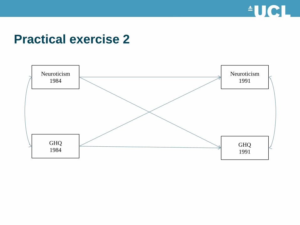
Mediation

X

Z

Y

Confounding

M

X

Y

Antecedent variable

X

M

Y

Moderator

Suppressor effects

• Association between X-Y usually decreases when adding

a confounder or mediator

– If it increases, this could indicate suppression

– Also known as ‘negative confounding’

• If regression coefficient larger than correlation, also

indicates suppression

• Also known as ‘inconsistent mediation’

– at least one indirect effect has a different sign than other indirect or

direct effects in a model

Suppression

• Verbal associated with mechanical

• Verbal not associated with success

• Mechanical B = 0.4

• Verbal B = -0.2

• Verbal ability is required for mechanical test

Mechanical

Pilot success

Verbal

Horst (1941) Mechanical Verbal Pilot success

Mechanical 1

Verbal 0.5 1

Pilot success 0.3 0 1

LATENT VARIABLES

Afternoon session

Measurement error

• Measurement error attenuates correlations

– In X variables, attenuates regression coefficients

– In Y variables, increases standard errors

• Latent variables are used to address measurement error

– If known, we can specify what it is

– If unknown, we can estimate from multiple indicators

Latent variables

• Captures covariation between observed

variables

– Intelligence, personality, SES

• Latent variable is common cause of indicators

• Advantages

– Reduces measurement error

– Address collinearity

– Invoke theoretical constructs

Latent

Observed

Observed

Observed

Other names for latent variables

• Hypothetical variables

• Hypothetical constructs

• Factors

• Unobservable variables

• Unmeasured variable influenced by causal indicators

• Phantom variables

• Variables which exist only in the mind of social scientists

Theoretical status of latent variables

• Formal

– Syntax: Defined by x1, x2, x3

– Semantics: 1 unit increase in f1, X unit increase in Y

• Empirical

– Does the model fit the data?

• Ontological

– The latent exists independent of measurement (entity realism),

observable in the future (e.g. atoms)

– The latent variable is constructed (constructivist)

– Operationalist (numerical track, empirical only)

Latent variable units

• There are no units

• Two solutions

– Fix a path coefficient to 1 (default = first)

– Fix variance of latent variable to 1

• Standardizes the latent so that 1 unit = 1 SD or z score

Path diagram notation

Observed

Latent

Regression

Correlation, covariance

Pathway added following modification index

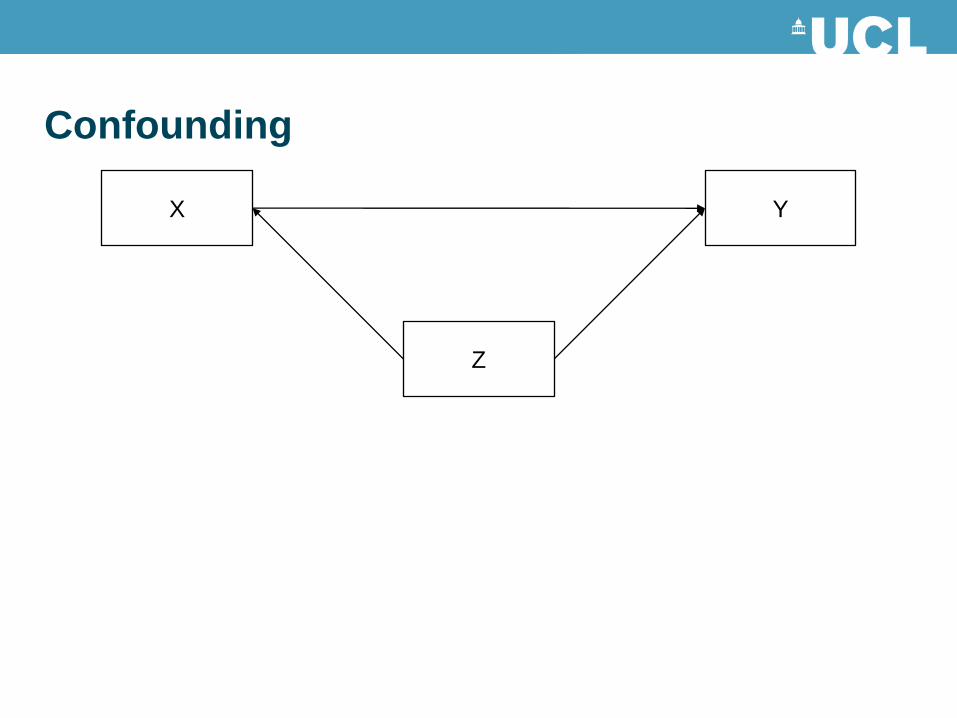
Measurement model

Latent

Observed

Observed

Observed

Latent

Observed

Observed

Observed

1 1

Structural model

Latent

Observed

Observed

Observed

Latent

Observed

Observed

Observed

1 1

exogenous endogenous

Confirmatory Factor Analysis

• Prior knowledge about factors

• More advanced stage of research

• Factors assumed to have caused correlations

• Specify exact model in advance

• Do the data fit the hypothesized model?

• Theory testing (CFA), not hypothesis generation (EFA)

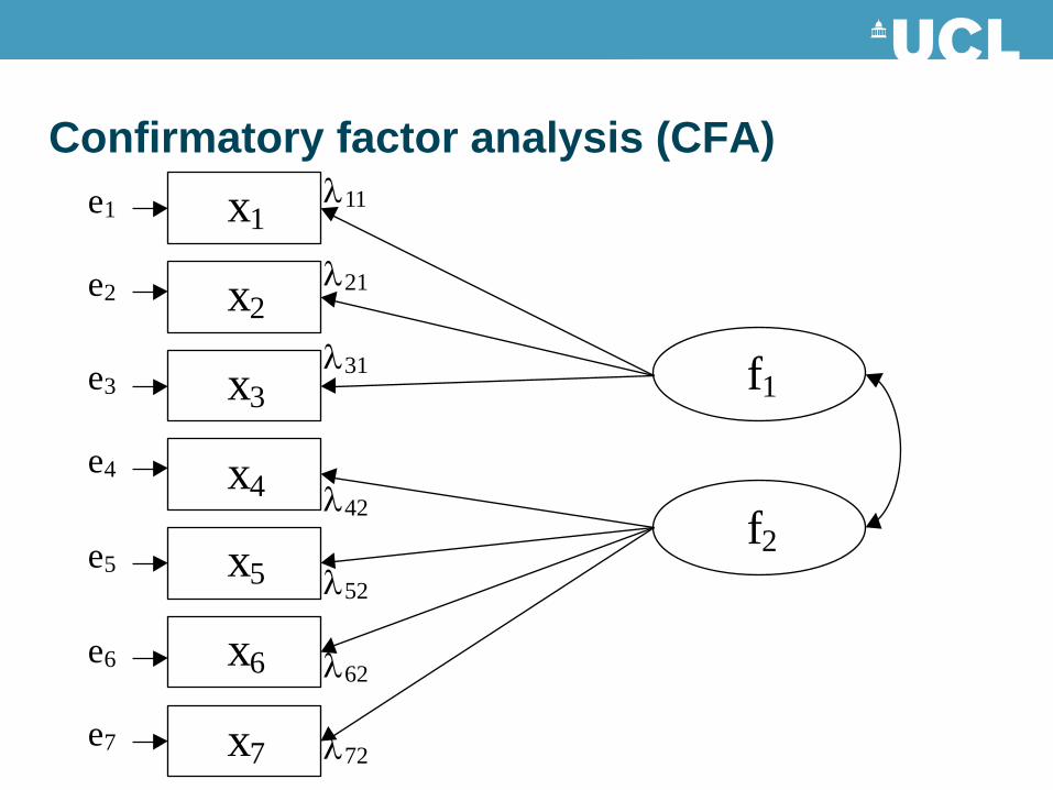
Confirmatory factor analysis (CFA)

x2

x3

x4

x5

x6

x1

x7

f1

f2

l11

l72

l31

l52

l21

l42

l62

e1

e2

e3

e4

e5

e6

e7

Exploratory factor analysis (EFA)

x2

x3

x4

x5

x6

x1

x7

f1

f2

l11

l12

l72

l71

l22

l31

l32

l41

l51

l52

l61

l21

l42

l62

e1

e2

e3

e4

e5

e6

e7

Causal inference

• Factors reflect underlying processes that create variables

– Implies that factors cause variables

• EFA

– What underlying processes could have produced the correlations?

– Useful in theory development

• CFA

– Are correlations consistent with hypothesized factor structure?

– Useful in theory testing

Measurement model steps

• Latent variables defined by observed variables

• At least three, preferably more

• Choose method for setting metric

– MODEL: iq BY verbal1 verbal2 maths english;

– MODEL: iq BY verbal1* verbal2 maths english; iq@1;

• Model testing using confirmatory factor analysis

• Test each latent variable separately for fit

• Build up to the full model

Intelligence as a latent variable (ACONF)

IQ IQ@1

Verbal 2

Maths

English

Verbal 1

1 Verbal 2

Maths

English

Verbal 1

Mplus defaults for CFA

• Factor loading of first variable after BY is fixed to one

• Factor loadings of other variables are estimated

• Residual variances are estimated

• Residual covariances are fixed to zero

• Variances of factors are estimated

• Covariance between the exogenous factors is estimated

Model fit

Model results

Modification indices

• english WITH verbal2;

Goodness of fit indices

• χ² (not recommended N>200)

• χ²/df ratio (no agreed standard)

• TLI (.90 good, >.95 better)

• CFI (.90 good, >.95 better)

• RMSEA (<.05 ‘close’)

• SRMR (<.10 good, <.06 better)

• Use with caution

– SEM can disprove a model

– It cannot prove a model

Sample Size

• Ratio 20 to 1

• Ratio 5 to 1

• 200 minimum

• Fewer if no latent variables

• Fewer with larger correlations

• Fewer for simpler models

• Power analysis

Comparing fit of nested models

• 2 times difference in LL values for two models

• LR = 2(LL2-LL1)

• df = number of parameters constrained (removed from the

model)

• Statistic is distributed as chi-square

Saving factor scores

• Descriptive

• Treat as observed in other models

• Rank people on factor

– Percentiles

• Proxy for latent variable

• Caution – depends on fit/quality of model

• SAVE: FILE IS fscores.dat; SAVE ARE FSCORES;

Structural equation modelling steps

• Model fit=S-Σ

– S = actual data, Σ = implied covariance matrix

• Maximum likelihood estimation

– Given data and model, what parameter values make the observed

data most likely?

• Model modification

– Lagrange Multiplier tests

– Wald tests (‘model trimming’)

• Regression coefficients

• Indirect effects

Identification

• Number of knowns = m(m+1)/2

– m = manifest (measured) variables

• Parameters

– Path coefficients, variances, covariances

• Identified if moments >=parameters

• Mplus gives a number to each parameter in the matrices

– Available by asking for OUTPUT: TECH1;

Notation for matrices

Symbol English

λ

Lambda Loadings for endogenous

variables

ɸ Psi Variances and covariances for

exogenous variables

β Beta Causal path

θ Theta Measurement errors for

endogenous variables

Parameters: Loadings

f1

y1

y2

y3

f2

y4

y5

y6

Lambda λ f1 f2

y1 0 0

y2 7 0

y3 8 0

y4 0 0

y5 0 9

y6 0 10

Parameters: Variances and covariances

f1

y1

y2

y3

f2

y4

y5

y6

Psi ɸ

f1 f2

f1 18

f2 0 19

Parameters: Causal paths (regressions)

f1

y1

y2

y3

f2

y4

y5

y6

Beta

β

f1 f2

f1 0 0

f2 17 0

Parameters: Measurement errors

f1

y1

y2

y3

f2

y4

y5

y6

Theta

θ

y1 y2 y3 y4 y5 y6

y1 11

y2 0 12

y3 0 0 13

y4 0 0 0 14

y5 0 0 0 0 15

y6 0 0 0 0 0 16

Not identified

• This model has 4 parameters

• 2(2+1)/2 = 3 knowns

f1

y1

y3

# Matrix

1 Lambda Loadings for endogenous variables

1 Psi Variances and covariances for endogenous variables

0 Beta Causal paths

2 Theta Measurement errors for endogenous variables

Just identified


• 3(3+1)/2 = 6 knowns

• Fit cannot be tested

# Matrix



0 Beta Causal paths


f1

y1

y2

y3

Over identified


• 4(4+1)/2 = 10 knowns

• Fit can be tested

# Matrix



0 Beta Causal paths


f1

y2

y3

y4

y1

Model modification

• Parsimony

– Remove non-significant pathways

– Starting with the lowest t value

– MODEL TEST: p1=1; !provides Wald test

• Better fit

– Add additional pathways

– MODINDICES provide Lagrange Multiplier Tests

• Describe your modifications transparently

Problems with model modification

• Capitalize on chance

• Rarely reported as happened

• Using p values to make decisions unwise

• Hypothesized model has now changed

• Equivalently well-fitting but different models

Lothian Birth Cohort Study (1936)

• Do childhood risk factors influence cardiovascular disease

risk (inflammation) in old age?

– Father’s social class

– Intelligence at age 11

Participants

• Lothian Birth Cohort (1936)

• Survivors from Scottish Mental Survey 1947

• Located and recruited 2004-2007

• N=1091 (548 men), age 68 to 71

C-reactive protein

• Distal causes

– SES in childhood (father’s social class)

– Intelligence at age 11

• Proximal causes

– Health behaviours, quality of life, own SES

– Pathophysiological causes

– Body mass index

• Own SES

Hypothesized model

IQ

at age 11

Father’s social class

BMI Log

CRP

Health

behaviours

SES

Quality of

life

Mplus input file, new additions

• DEFINE: lncrprot1=ln(crprot1); units=unitwk1/10;

• MODEL:

• ses BY highered* higherclass lowerdep WHOQOL4;

ses@1; !WHOQOL4 added

• hb BY smokcat1* phyactiv f2 units; hb@1;

• who BY WHOQOL1* WHOQOL2-WHOQOL4; who@1;

WHOQOL3 WITH WHOQOL2;

Indirect pathways

• MODEL INDIRECT:

• lncrprot1 IND bmi1 ses AGE11IQ;

• lncrprot1 IND hb ses AGE11IQ;

• lncrprot1 IND hb AGE11IQ;

• lncrprot1 IND BMI1 who;

• lncrprot1 IND f4 ses AGE11IQ;

• lncrprot1 IND bmi1 ses hfclass;

• lncrprot1 IND hb ses hfclass;

• lncrprot1 IND hb hfclass;

• lncrprot1 IND BMI1 who;

• lncrprot1 IND f4 ses hfclass;

IQ

at age 11

Higher father’s

social class

Occupational social

class

Educational

attainment

Lower area-based

deprivation

Environmental

domain

Social

domain

Psychological

domain

Physical

domain

Smoking Health aware

dietary pattern

Physical

activity

BMI Log

CRP

Alcohol

units

Sweet foods

dietary pattern

Quality of

life

Health

behaviours

SES

.80

.66

.57

.29

-.38 .28 .63

.60 .79 .56 .67

.36

.11

.25

.55

-.18

-.39

-.17

.14

.14

.23

-.13

.07

-.07

-.09

-.26

.09

.19

-.46

.22

PRACTICAL SESSION

MODEL EXTENSIONS

Appendices

Formative indicators

• Latent variables with reflective indicators

– Construct causes the variables

• Latent variables with formative indicators

– Indicators cause the construct

• SES a good example

– Which model is more believable?

Hagger-Johnson G et al. J Epidemiol Community Health

doi:10.1136/jech.2010.127696

Formative indicators

• MODEL:

f2 BY verbal1 verbal2 maths english;

ses BY f2*;

ses@0;

ses ON occupation@1 education income;

Categorical outcomes

• CATEGORICAL ARE smoker84;

X

M

U

Time to event data (survival analysis)

• SURVIVAL = t_all;

• TIMECENSORED = eventall (1 = NOT 0 = RIGHT);

• ANALYSIS: BASEHAZARD = OFF;

• TYPE=RANDOM;

• MODEL:

• t_all ON agyrs sex smoker84 n84;

X T

X1

M

Y

X2

Moderated mediation

Example of suppression

• Simple regression shows a positive association between BP and birth

weight: the regression coefficient for birth weight is 1.861 mmHg/Kg

(95% CI: 0.770, 2.953).

• Simple regression also reveals a positive association between BP and

current weight: the regression coefficient for current weight is 0.382

(95% CI = 0.341, 0.423) mmHg/Kg.

• BP is regressed on birth weight and current weight simultaneously and

the partial regression coefficients for birth weight and current weight

are -3.708 (95% CI = -4.794, -2.622) and 0.465 (95% CI = 0.418,

0.512) mmHg/Kg respectively, and both are highly statistically

significant

• Adjusting for a mediator? birth weight → BP

Nine scenarios

Population value of direct effect

0 Positive Negative

Population

value of third

variable effect

0 * * *

Positive Fully

mediated or

confounded

*

Partly

mediated or

confounded

*

Suppression

Negative Fully

mediated or

confounded

*

Suppression

*

Partly

mediated or

confounded

*

*Possible by chance

Suppression is also called ‘inconsistent mediation’ or ‘negative confounding’.

Mediation or confounding may also be called mediation or ‘positive

confounding’.

Other terms used

Zhao et al. (2010) terms

Complementary mediation Mediated effect ab and direct effect c

exist and in same direction

Competitive mediation Mediated effect ab and direct effect c

exist and in opposite directions

Indirect-only mediation Mediated effect ab exists

No direct effect c

Direct-only non-mediation Direct effect c exists, no significant ab

No-effect non-mediation Neither direct nor indirect exists

References and further reading

• Baron, R. M. and Kenny, D. A. (1986). The moderator-mediator variable distinction in social psychological research: conceptual, strategic, and

statistical considerations. Journal of Personality and Social Psychology, 51, 1173-1182.

• Ben-Shlomo, Y. and Kuh, D. (2002). A life course approach to chronic disease epidemiology: conceptual models, empirical challenges and

interdisciplinary perspectives. International Journal of Epidemiology, 31, 285-293.

• Bollen, K. A. (2002). Latent variables in psychology and the social sciences. Annual Review of Psychology, 53, 605-634.

• Borsboom, D., Mellenbergh, G. J., and van Heerden, J. (2003). The theoretical status of latent variables. Psychological Review, 110, 203-219.

• Byrne, B. M. (2011). Structural Equation Modeling with Mplus: Basic Concepts, Applications, and Programming. London: Routledge.

• Cox, B. D. (1988). Health and Lifestyle Survey, 1984-1985 (HALS1) User Manual. Economic and Social Data Service.

• Deary, I. J., Blenkin, H., Agius, R. M., Endler, N. S., Zealley, H., and Wood, R. (1996). Models of job-related stress and personal achievement

among consultant doctors. British Journal of Psychology, 87, 3-29.

• Hagger-Johnson, G., Mõttus, R., Craig, L. C. A., Starr, J. M., & Deary, I. J. (in press). Pathways from childhood intelligence and socio-

economic status to late-life cardiovascular disease risk. Health Psychology.

• Hayes, A. F. (2009). Beyond Baron and Kenny: Statistical mediation analysis in the new millennium. Communication Monographs, 76, 408-

420.

• Judd, C. M. and Kenny, D. A. (1981). Process analysis. Evaluation Review, 5, 602-619.

• Kline, R. B. (2005). Principles and Practice of Structural Equation Modeling (2nd . London: Guilford Press.

• Kuh, D., Ben-Shlomo, Y., Lynch, J., Hallqvist, J., and Power, C. (2003). Life course epidemiology. Journal of Epidemiology and Community

Health, 57, 778-783.

• Leon, D. A., Lawlor, D. A., Clark, H., and Macintyre, S. (2006). Cohort profile: The Aberdeen children of the 1950s study. International Journal

of Epidemiology, 35, 549-552.

References and further reading

• Lockhart, G., MacKinnon, D. P., and Ohlrich, V. (2011). Mediation analysis in psychosomatic medicine research. Psychosomatic Medicine, 73,

29-43.

• MacKinnon, D. P., Fairchild, A. J., and Fritz, M. S. (2007). Mediation analysis. Annual Review of Psychology, 58, 593-614.

• MacKinnon, D. P., Krull, J. L., and Lockwood, C. M. (2000). Equivalence of the mediation, confounding and suppression effect. Prevention

Science, 1, 173-181.

• Mathieu, J. E. and Taylor, S. R. (2006). Clarifying conditions and decision points for mediational type inferences in organizational

behavior. Journal of Organizational Behavior, 27, 1031-1056.

• Selig, J. P. and Preacher, K. J. (2009). Mediation models for longitudinal data in developmental research. Research in Human Development,

6, 144-164.

• Singh-Manoux, A., Martikainen, P., Ferrie, J., Zins, M., Marmot, M., and Goldberg, M. (2006). What does self rated health measure? results

from the British Whitehall II and French Gazel cohort studies. Journal of Epidemiology and Community Health, 60, 364-372.

• Smith, T. W. (2006). Personality as risk and resilience in physical health. Current Directions in Psychological Science, 15, 227-231.

• Tabachnick, B. G. and Fidell, L. S. (2006). Using Multivariate Statistics (5th Edition). London: Pearson. [chapter 14]

• Tu, Y. K., Gunnell, D., and Gilthorpe, M. (2008). Simpson's paradox, lord's paradox, and suppression effects are the same phenomenon - the

reversal paradox. Emerging Themes in Epidemiology, 5(1):2+.

• World Health Organization (2002). The world health report 2002 - Reducing Risks, Promoting Healthy Life. World Health Organization,

Geneva.

• Wright, S. (1934). The Method of Path Coefficients. Annals of Mathematical Statistics, 5, 161-215.

• Zhao, X., John, and Chen, Q. (2010). Reconsidering Baron and Kenny: Myths and truths about mediation analysis. Journal of Consumer

Research, 37:197-206.

•

Latent variable structural equation models for ... · PDF fileLatent variable structural...

Documents

Transcript of Latent variable structural equation models for ... · PDF fileLatent variable structural...