Latent variable models forlongitudinal twin data

Annica Dominicus

Mathematical StatisticsDepartment of Mathematics

Stockholm University2006

Doctoral Dissertation 2006Mathematical StatisticsStockholm UniversitySE-106 91 Stockholm

c©Annica DominicusISBN 91-7155-211-1 pp. 1-49Printed by Akademitryck AB

Abstract

Longitudinal twin data provide important information for explor-ing sources of variation in human traits. In statistical models fortwin data, unobserved genetic and environmental factors influenc-ing the trait are represented by latent variables. In this way, traitvariation can be decomposed into genetic and environmental com-ponents. With repeated measurements on twins, latent variablescan be used to describe individual trajectories, and the genetic andenvironmental variance components are assessed as functions of age.This thesis contributes to statistical methodology for analysing lon-gitudinal twin data by (i) exploring the use of random change pointmodels for modelling variance as a function of age, (ii) assessing hownonresponse in twin studies may affect estimates of genetic and en-vironmental influences, and (iii) providing a method for hypothesistesting of genetic and environmental variance components. The ran-dom change point model, in contrast to linear and quadratic randomeffects models, is shown to be very flexible in capturing variabilityas a function of age. Approximate maximum likelihood inferencethrough first-order linearization of the random change point modelis contrasted with Bayesian inference based on Markov chain MonteCarlo simulation. In a set of simulations based on a twin model forinformative nonresponse, it is demonstrated how the effect of non-response on estimates of genetic and environmental variance com-ponents depends on the underlying nonresponse mechanism. Thisthesis also reveals that the standard procedure for testing variancecomponents is inadequate, since the null hypothesis places the vari-ance components on the boundary of the parameter space. Theasymptotic distribution of the likelihood ratio statistic for testingvariance components in classical twin models is derived, resultingin a mixture of chi-square distributions. Statistical methodology isillustrated with applications to empirical data on cognitive functionfrom a longitudinal twin study of aging.

Keywords: Latent variable models; twin models; variance compo-nents; change point models; non-ignorable nonresponse; likelihoodratio tests.

iv

Preface

This thesis has been prepared during my enrollment as a PhDstudent at the Division of Mathematical Statistics, Department ofMathematics, Stockholm University. Much of the work has takenplace at the Department of Medical Epidemiology and Biostatistics(MEB), Karolinska Institutet. As part of my PhD studies I spentone semester at the Department of Biostatistics, Harvard School ofPublic Health. It has been a very rewarding and enjoyable time,which is much thanks to all the people who have shared ideas, ex-periences and everyday life with me during these years. I wouldlike to express my sincere gratitude to all these people: former andcurrent colleagues, family and friends, who have contributed in oneway or another to this thesis. In particular, I would like to thank:

Juni Palmgren, my main supervisor, for all the encouragement andsupport, and for giving me a broad perspective on biostatistics andresearch. Your enthusiasm, energy and optimism has been my guid-ing star!

Nancy Pedersen, my co-supervisor, for support, brilliant guidance,and for always looking out for my best interests. Thanks for havingpatience with me, and for helping me to get back on track wheneverI needed it.

Anders Skrondal, my co-author, for agreeing to visit Stockholm inthe first place, and for fruitful collaboration.

Hakon Gjessing, my co-author, for fun and fruitful discussions, andfor valuable contributions.

Samuli Ripatti, my co-author, for enjoyable collaboration and forteaching me the beauty of being pragmatic.

All my colleagues and friends at Matstat, for making Kraftriket agood place to be. Especially, I thank Rolf Sundberg, for showinginterest in my work and for giving constructive comments on a latedraft of the thesis, Ola Hossjer, for good discussions, and ChristinaNordgren, for always being very friendly and helpful.

v

All my colleagues and friends at MEB, and especially everyone inthe Biostat group, for contributing to the good and friendly atmo-sphere. In particular, I want to thank Yudi Pawitan and Paul Dick-man for important contributions to making theoretical and appliedwork in the Biostat group so rewarding, Anna Johansson, AnnaTorrang, Asa Klint and Gudrun Jonasdottir for discussions andlaughs, and Alexander Ploner and Sven Sandin for always beingvery helpful.

All twin researchers working with SATSA, for interesting and valu-able discussions.

Everyone at the Department of Biostatistics, Harvard School of Pub-lic Health, for making my stay in Boston very rewarding and enjoy-able.

My nearest and dearest. My father, Bengt, my mother, Maud, andmy ‘extra’, Stefan, for unconditional love and continuous support.My words of appreciation also go to my dear brothers Eric, Larsand Gustaf, as well as everyone else in the family and all friends. Aspecial ‘thank you’ goes to Magnus, my hero, for invaluable supportand for your marvelous ability to put things in perspective.

The Swedish Foundation of Strategic Research, the Swedish Foun-dation for International Cooperation in Research and Higher Edu-cation, the National Institutes of Health, the Department of HigherEducation, the Swedish Scientific Council, and the Swedish Councilfor Social Research, for financial support.

Stockholm, February 2006,Annica Dominicus

vi

List of papers

This thesis is based on the following papers, which are referred toin the text by their Roman numerals:

I Dominicus, A., Ripatti, S., Pedersen, N.L. and Palmgren, J.Modelling variability in longitudinal data using random changepoint models. Submitted.

II Dominicus, A., Palmgren, J. and Pedersen, N.L. Bias in vari-ance components due to nonresponse in twin studies. TwinResearch and Human Genetics. In press.

III Dominicus, A., Skrondal, A., Gjessing, H.K., Pedersen, N.L.and Palmgren, J. Likelihood ratio tests in behavioral genetics:Problems and solutions. Behavior Genetics. In press.

Previously published papers were reprinted with permission of Aus-tralian Academic Press (Paper II) and Springer (Paper III).

vii

viii

Contents

1 Introduction 1

2 Swedish Adoption/Twin Study of Aging 4

3 Latent variable models 73.1 Models for twin data . . . . . . . . . . . . . . . . . . 73.2 Models for longitudinal data . . . . . . . . . . . . . . 103.3 Models for longitudinal twin data . . . . . . . . . . . 12

3.3.1 Latent growth curve models . . . . . . . . . . 133.3.2 Linear latent variable models . . . . . . . . . 153.3.3 Variance profiles . . . . . . . . . . . . . . . . 16

4 Likelihood inference 184.1 Maximum likelihood estimation . . . . . . . . . . . . 18

4.1.1 The likelihood . . . . . . . . . . . . . . . . . . 184.1.2 Linear latent variable models . . . . . . . . . 184.1.3 Nonlinear latent variable models . . . . . . . . 19

4.2 Goodness-of-fit . . . . . . . . . . . . . . . . . . . . . 214.2.1 Asymptotic likelihood theory . . . . . . . . . 214.2.2 Tests of hypotheses on the boundary . . . . . 224.2.3 Likelihood ratio tests of variance components 244.2.4 Likelihood ratio tests of nested twin models . 264.2.5 Model selection based on relative fit criteria . 28

5 Bayesian inference 305.1 Three-stage hierarchical models . . . . . . . . . . . . 305.2 MCMC for the hierarchical change point model . . . 31

6 Dropout from longitudinal twin studies 336.1 Missing value mechanisms . . . . . . . . . . . . . . . 336.2 Ignorable dropout . . . . . . . . . . . . . . . . . . . . 356.3 Modelling the dropout process . . . . . . . . . . . . . 356.4 Dropout due to death . . . . . . . . . . . . . . . . . . 37

7 Discussion 38

8 Svensk sammanfattning 41

ix

References 43

Paper I: Modelling variability in longitudinal datausing random change point models

Paper II: Bias in variance components due to nonre-sponse in twin studies

Paper III: Likelihood ratio tests in behavioral genet-ics: Problems and solutions

x

1 Introduction

Genetic and environmental influences on human traits can be ex-plored by comparing the resemblance in trait values for differentkinds of relatives. In twin studies, a larger trait resemblance amongidentical twins compared to fraternal twins is interpreted as an ef-fect of genes. Because genes can be turned on and off in differentphases of life and environmental factors change through accumula-tion or removal, genetic and environmental influences may not bethe same throughout life. Longitudinal twin studies offer an excep-tional possibility to explore these issues.

The classical twin model can be formulated as a structural equa-tion model (e.g. Bollen, 1989), where unobserved genetic and envi-ronmental factors are represented by latent variables (random vari-ables) with a specified probability distribution. This enables aninvestigation of sources of individual variability. Random variablescan also be used for describing variability and dependence in re-peated measurements on individuals, in so called random effectsmodels (e.g. Laird and Ware, 1982). In latent growth curve modelsfor longitudinal twin data, these ideas are combined by incorporat-ing genetic and environmental factors influencing the overall levelof an individual’s outcome (trait), as well as factors influencing thetemporal development (e.g. McArdle, 1986).

This thesis addresses various aspects of statistical methodologyfor analysing longitudinal twin data. It consists of an introductorypart and three original papers. The introductory part is a broadsynthesis of the topic area placing the papers in a broader context.The work has been guided by the general aim of improving methodsfor the statistical analysis of data from the Swedish Adoption/TwinStudy of Aging (SATSA) (Finkel and Pedersen, 2004). Empiricaldata on cognitive function from this study are used to illustratestatistical methodology. Cognitive function is measured on contin-uous scales and the twin models considered in the thesis are formultivariate normally distributed outcomes.

A central goal when analysing longitudinal twin data is to de-compose the trait variance profile over age into genetic and envi-ronmental variance components. This can be achieved by formulat-ing a growth curve model for the individual trajectories, including

1

assumptions about variability and co-variability of features of thecurves. Because the shape of the variance profile is restricted by thegrowth curve model, it is crucial that the growth curve model doesnot only reflect the change in mean trait level over age but also thechange in trait variance with age.

The aim of Paper I is to formulate a longitudinal model that isflexible for modelling changes in trait variability. We consider a ran-dom change point model for modelling cognitive decline in old age,and compare it to linear and quadratic random effects models. Dueto the nonlinearity of the random change point model, parameterestimation is not straightforward. We contrast approximate max-imum likelihood inference based on first-order linearization of therandom change point model (Beal and Sheiner, 1982), with Bayesianinference based on Markov chain Monte Carlo (MCMC) simulationusing Gibbs sampling (Geman and Geman, 1984).

In longitudinal twin studies, loss to follow-up (dropout) of someparticipants is often a reality, which means that the available dataare incomplete. Estimation of genetic and environmental variancecomponents based on incomplete twin data is commonly based onfull information maximum likelihood (FIML), assuming that thedropout mechanism is ignorable (Little and Rubin, 2002). In studiesof aging, loss to follow-up due to death is likely to occur, and thisis also the case in SATSA. Dropout due to death is believed tobe related to the aging process, which makes the nonresponse inSATSA problematic (Pedersen et al., 2003).

The aim of Paper II is to clarify the meaning of ignorable non-response in twin studies and assess how non-ignorable nonresponsemay influence estimates of genetic and environmental variance com-ponents. In a set of simulations, we investigate if the decrease in es-timates of genetic variance components with time, which is observedin analyses of cognitive function in SATSA, may be attributable tothe dropout of study participant.

Assessments of genetic and environmental influences based ontwin data are usually based on likelihood inference. Statistical testsrely on standard asymptotic theory. However, tests of genetic or en-vironmental variance components correspond to tests of hypotheseson the boundary of the parameter space, since variance componentsare naturally constrained to be non-negative. Hence, the test of

2

variance components is a nonstandard problem and the methodscommonly used are inappropriate.

Paper III raise this question and provide a method for makingcorrect inference. Based on asymptotic likelihood theory for testingparameters on the boundary of the parameter space (Self and Liang,1987), we derive the asymptotic distribution of the likelihood ratiostatistic for tests of genetic and environmental variance componentsin classical twin models.

A more detailed background to Papers I to III is given in thefollowing sections. In section 2, the Swedish Adoption/Twin Studyof Aging is presented. Section 3 describes the ideas underlying la-tent variable modelling of twin data, longitudinal data, and longi-tudinal twin data. Likelihood inference for latent variable modelsis described in section 4, and is contrasted with Bayesian inferencethrough MCMC simulation in section 5. Dropout from twin studies,and nonresponse in general, is discussed in section 6. Conclusionsand final remarks are given in section 7.

3

2 Swedish Adoption/Twin Study of Aging

The Swedish Adoption/Twin Study of Aging (SATSA) is a longi-tudinal twin study including both questionnaire assessments andin-person testing of cognitive and functional capabilities, personal-ity and health. The base population of SATSA consists of 3838individuals, comprising all twin pairs in the Swedish Twin Registry(Lichtenstein et al., 2002) who indicated that they had been sepa-rated before the age of eleven years and reared apart, and a sampleof twins reared together matched on the basis of gender, date andcounty of birth. The first in-person testing in SATSA took place in1986-1988 for a subsample of pairs and follow-up data were obtainedafter 3, 6, 13 and 16 years. SATSA has been described in detail byFinkel and Pedersen (2004).

In this thesis, cognitive measures are used as markers of the agingprocess. The SATSA cognitive test battery includes eleven cogni-tive measures drawn from various sources and chosen to assess fourareas of cognitive ability: crystallized intelligence, fluid intelligence,memory and perceptual processing speed (Pedersen et al., 1992).Crystallized intelligence refers to those cognitive processes that areimbedded in a context of cultural meaning and reflects the store ofknowledge or information that has accumulated over time. Fluid in-telligence is the on-the-spot reasoning ability, which is not basicallydependant on an individual’s experience. Perceptual speed is theability to quickly and accurately compare letters, numbers, objects,pictures, or patterns.

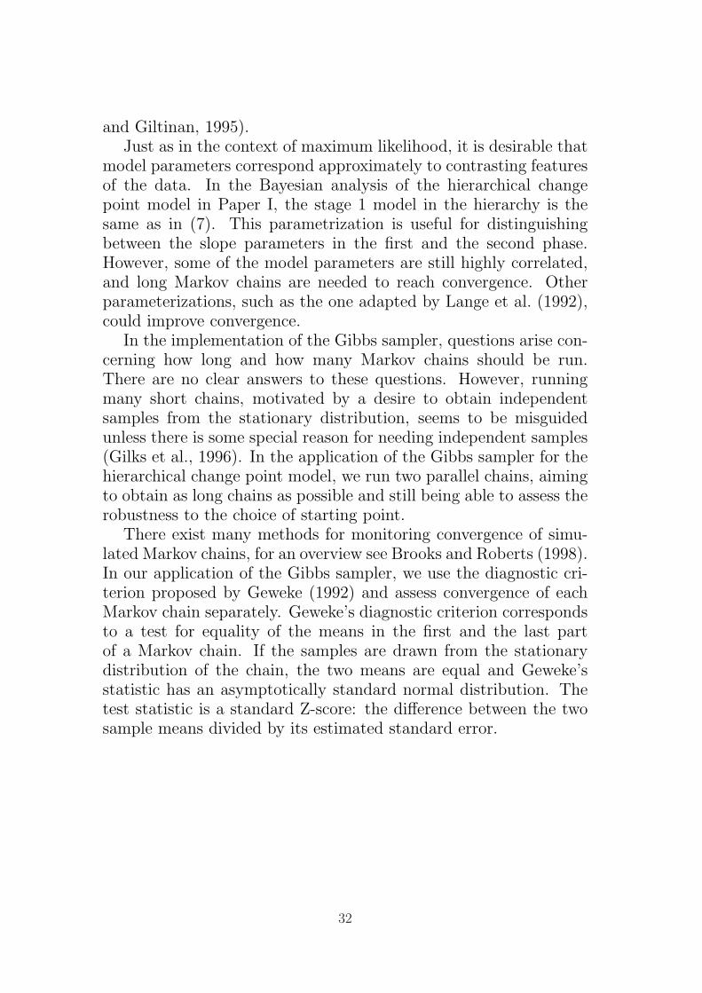
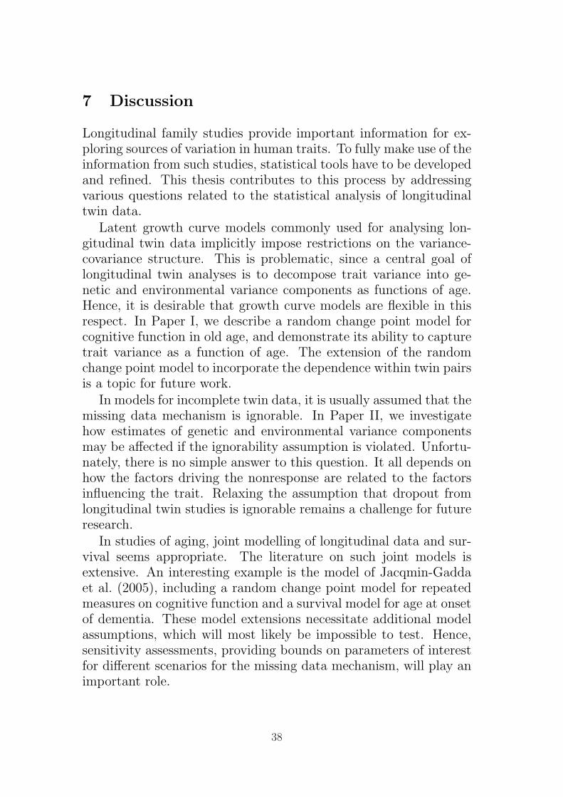
Only one cognitive measure at a time is used to illustrate statis-tical methodology addressed in this thesis. In Paper III the BlockDesign test, tapping fluid ability, is used for illustration. In Pa-pers I and II we use the Symbol Digit test, which is a measure ofperceptual speed. The bivariate distribution of Symbol Digit testscores for twins, stratified on zygosity, is shown in Figure 1. Withthe purpose of giving a rough idea of the distribution, test scoresfrom all five test occasions are included and treated as independent.The picture indicates that the within-pair correlation for identical(monozygotic, MZ) twins is higher than for fraternal (dizygotic, DZ)twins, suggesting a genetic influence on perceptual speed.

The repeated measures of cognition in SATSA are unbalanced in

4

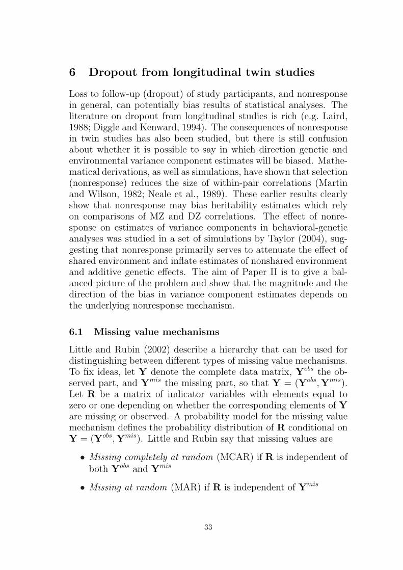
the sense that individuals are measured at different ages. One rea-son for the unbalance is the study design, with participants being50 years or older at study entry. The only exception to this rule isa subsample of twins younger than 50 years, who were recruited foranother study and also were administered the same cognitive bat-tery. Another reason for the unbalance is that some participants arelost to follow-up or have intermittent missing values. The dropoutmechanism is believed to be related to the process of aging andcognitive decline (Pedersen et al., 2003; Dominicus, 2003). Figure2 displays cognitive trajectories for a random subsample of SATSAparticipants, stratified on participation pattern. The first groupconsists of individuals with test scores from 5 occasions, and theother groups include individuals who drop out from the study afterparticipating at 4, 3 and 2 occasions, respectively. The figure showsthat the age distribution is somewhat different for these groups.There is also an indication that the distribution of the overall level,and temporal development, of cognitive function may be differentas well, although the pattern is not clear.

MZ twin pairs

Twin 1

Tw

in 2

10 30 50

1030

50

DZ twin pairs

Twin 1

Tw

in 2

10 30 50

1030

50

Figure 1: Contour level plots for Symbol Digit test scores.

5

50 60 70 80

10

40

70

5 occasions

50 60 70 80

10

40

70

4 occasions

50 60 70 80

10

40

70

3 occasions

50 60 70 80

10

40

70

2 occasions

Age

Sym

bo

l D

igit t

est

sco

re

Figure 2: Trajectories of Symbol Digit test scores for a random subsample ofSATSA participants stratified on participation pattern.

6

3 Latent variable models

3.1 Models for twin data

Based on trait data from monozygotic (MZ) and dizygotic (DZ)twins, genetic and environmental influences can be dissected with-out having any molecular genetic, or environmental, data. This ispossible through the formulation of models including latent vari-ables representing unobserved genetic and environmental factors.To fix ideas, consider an univariate trait measured on a continu-ous scale. Genes can have an additive effect on the trait, or showa dominance deviation. The latter reflects the extent to which agenetic variant (allele) does not simply ‘add up’ if it is present inzero, one or two copies in the chromosome pair. For the jth twin(j = 1, 2) in the ith twin pair (i = 1, ..., n), let ηAij and ηDij denotethe additive and the dominant genetic influences on the trait, Yij.Environmental influences can be either shared within twin pairs orindividual-specific, and these components are denoted ηCij and ηEij,respectively. The model is expressed as

Yij = xijβ + λAηAij + λDηDij + λCηCij + λEηEij, (1)

where β is a vector of regression coefficients (including an inter-cept), xij is the associated vector of covariates, and λA, λD, λC

and λE are factor loadings (path coefficients) for the unobservedgenetic and environmental factors. The latent variables ηAij, ηDij,ηCij and ηEij are assumed to be normally distributed with meanzero and variances VA, VD, VC and VE, respectively. The normalitydistribution is a consequence of the central limit theorem under theassumption that a large number of genetic and environmental influ-ences are present, all effects being small and largely independent ofeach other (Lange, 1978).

Some of the random components in (1) are correlated between rel-atives. Assuming random mating and Hardy–Weinberg equilibriumin the population, the within-pair correlation of genetic factors forrelatives can be derived. MZ twins share all their segregating genes,so the genetic correlations, ρ(ηAi1, ηAi2) and ρ(ηDi1, ηDi2), are bothequal to one. In contrast, DZ twins share on average only half oftheir segregating genes, and it can be shown that ρ(ηAi1, ηAi2) = 0.5and ρ(ηDi1, ηDi2) = 0.25 (e.g. Falconer and Mackay, 1996).

7

Environmentally caused similarity for twins reared in the samefamily is assumed to be the same for MZ and DZ twins, that is,ρ(ηCi1, ηCi2) = 1 for all twin pairs. The equal environments as-sumption is of course crucial for the interpretation of findings intwin studies. It has been tested in several ways and appears rea-sonable for most traits (Plomin et al., 2001, pp. 79–82).

Model (1) can be parameterized in terms of the variances VA, VD,VC and VE, by setting the factor loadings λA, λD, λC and λE to one.Alternatively, the model can be parameterized in terms of the factorloadings λA, λD, λC and λE, by fixing the variances VA, VD, VC andVE to one. The latter is the parametrization commonly used becauseit ensures that estimated variance components are non-negative, andcan be directly interpreted as genetic and environmental influencescontributing to the heterogeneity between individuals.

If the genetic and environmental factors are independent andnormally distributed then the trait Yij is normally distributed withthe following mean and variance-covariance structure:

E(Yij) = xijβ for all twins

Var(Yij) = λ2A + λ2

D + λ2C + λ2

E for all twins

Cov(Yi1, Yi2) = λ2A + λ2

D + λ2C for MZ twins

Cov(Yi1, Yi2) = 0.5λ2A + 0.25λ2

D + λ2C for DZ twins.

It is not possible to estimate all four variance components λ2A, λ2

D,λ2

C and λ2E from the equations above. One solution is to compare

several constrained models based on indices of fit such as the Akaikeinformation criterion (AIC) (Akaike, 1987). Often the dominantgenetic effect is excluded and the genetic effect thus assumed to besolely additive. The model, referred to as the ACE model (Nealeand Cardon, 1992), has the form

Yij = xijβ + λAηAij + λCηCij + λEηEij. (2)

Like model (1), model (2) assumes that many independent in-fluences are present and that neither Gene-Environment correlationnor Gene-Environment interaction is present. Gene-Environmentcorrelation means that for some loci, the distribution of the allelesis associated with environmental factors. Gene-Environment inter-action refers to the case where the effect of some genes is associ-ated with the exposure to some environmental factors or vice versa.

8

Purcell (2002) extends model (2) by relaxing the assumptions of nointeraction, and no correlation, between genes and environment.

The twin model, as formulated in (2), belongs to the family ofstructural equation models (SEM) (see e.g. Bollen, 1989). It caneasily be extended to more complex data structures. An importantfeature of model (2) is that the variation for MZ and DZ twins isconstrained to be equal. In contrast, early methods for the sta-tistical analysis of twin data were based on the idea of dissectingtrait variance into between-pair and within-pair components in ananalysis of variance (ANOVA). If there is a genetic influence, thewithin-pair variation is smaller among MZ twins than among DZtwins (e.g. Sham, 1998). A general framework for variance decom-position into within-pair and between-pair components are based onmultilevel models, including latent variables corresponding to dif-ferent levels of clustering (see e.g. Hox, 2002). By restricting thesum of within-pair and between-pair variance to be the same forMZ and DZ twins in a multilevel model for twin data, estimatesof genetic and environmental variance components similar to thosein the SEM formulation can be obtained (McArdle and Prescott,2005).

Conclusions about a general population based on findings in twinstudies relies on the assumption that the marginal trait distributionof twins is representative for the trait distribution of individuals inthe general population. Although twins differ from individuals inthe general population for some traits, such as birth weight, this isnot believed to be the case for most phenotypes.

9

3.2 Models for longitudinal data

Longitudinal data arise when responses (trait values) for each indi-vidual are available on multiple occasions. The dependence amongmeasurements from the same individual can be accommodated inseveral ways. Unobserved heterogeneity between individuals in-duces within-individual dependence, which can be accounted forby including individual-specific latent variables in the model. Thisapproach uses a combination of (across individuals) fixed effects tosummarize the average features of the trajectories and individual-specific random effects (with some specified probability distribution)to represent variability between individuals.

In the random intercept model, an individual-specific interceptaccounts for the association between measurements from the sameindividual. Extensions of this model to random coefficient modelsallow both the level of the response and the effects of covariatesto vary randomly across individuals (e.g. Laird and Ware, 1982).A useful version of the random coefficient model for longitudinaldata is the growth curve model where individuals are assumed todiffer not only in their intercepts but also in other aspects of theirtrajectory over time. These models include random coefficients for(functions of) time. Let Yjk denote the response of the jth individualat time point tjk (k = 1, ..., nj). This notation allows for unbalanceddata. The linear growth curve model is expressed as

Yjk = βI + tjkβS + ηIj + tjkηSj + εjk, (3)

where βI and βS are fixed effects, ηIj and ηSj are individual-specificrandom effects, and εjk is an error term. In vector notation, model(3) is expressed as

Yj = Xjβ + Λjηj + εj, (4)

where Yj = (Yj1, ..., Yjnj)T , εj = (εj1, ..., εjnj

)T , β = (βI , βS)T ,

ηj = (ηIj, ηSj)T , and Xj = Λj =

(1 · · · 1tj1 · · · tjnj

)T

, with ηj and

εj random. The model specification involves specifying probabilitydistributions for the random effects, ηj, and the error terms, εj.For multivariate normal data, the random effects are assumed to

10

be multivariate normally distributed with mean zero and variance-covariance matrix Ψ, and the error terms are multivariate normallydistributed with mean zero and variance-covariance matrix Φ. Ifresponses from the jth individual are independent, conditional onthe individual-specific random effects, the error terms in εj are inde-pendent and Φ thus a diagonal matrix. Deviations from conditionalindependence can be accounted for by including a serial correlationbetween error terms (e.g. Verbeke and Molenberghs, 2000).

Model (4) assumes a linear relationship between the responses,Yj, and the random effects, ηj. A generalization to nonlinear re-lationships between Yj and ηj is the family of generalized linearmixed models (GLMM) (e.g. Breslow and Clayton, 1993; Diggleet al., 2002). GLMMs are extensions of generalized linear mod-els (McCullagh and Nelder, 1989), to models with random effectsamong the predictor variables. Let µj denote the expected valueof Yj conditional on ηj. In GLMMs, µj is related to the linearpredictor via the link function g(·):

g(µj) = Xjβ + Λjηj. (5)

In addition to the specification of the link function, a probabilitydistribution for the random effects, ηj, has to be specified.

Other generalizations of model (4) are the nonlinear mixed mod-els (hierarchical nonlinear models) (e.g. Davidian and Giltinan, 1995).In vector notation, such models can be expressed as

Yj = f(Xj, ηj, β,Λj) + εj, (6)

where f(·) is any nonlinear function. Going from a linear to a non-linear function introduces various complications along the road. Afundamental difference between the linear and the nonlinear ver-sions of the mixed model lies in the ability to explicitly derive themarginal distribution of Yj. This is possible for the linear modelbut not for the nonlinear model, which complicates the estimation ofmodel parameters. The nonlinearity also complicates the interpre-tation of model parameters. In the linear mixed model, the fixed ef-fects, β, have the interpretation as ‘mean effects’, that is, the valuesproducing the ‘typical’ response vector at the covariate setting Xj.In contrast, in the nonlinear mixed model the mean response vector

11

for a given individual with covariate setting Xj is f(Xj, ηj, β,Λj),and the corresponding variation in the population of response vec-tors Yj (j = 1, ..., n for n individuals) depends on the assumptionsmade about ηj and f(·). In general,

E(f(Xj, ηj, β,Λj)) 6= f(Xj, β,Λj).

Hence, using the same function f(·) to model either individual meanresponse or population mean response does not in general lead tothe same marginal model for the population.

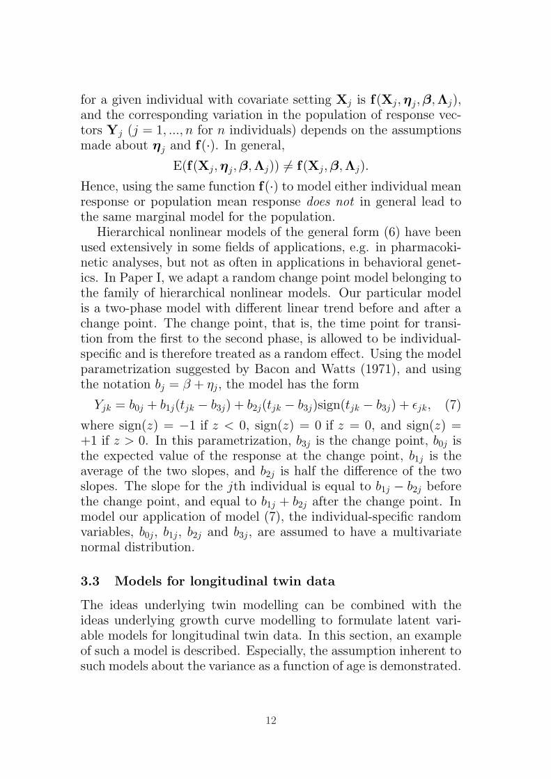
Hierarchical nonlinear models of the general form (6) have beenused extensively in some fields of applications, e.g. in pharmacoki-netic analyses, but not as often in applications in behavioral genet-ics. In Paper I, we adapt a random change point model belonging tothe family of hierarchical nonlinear models. Our particular modelis a two-phase model with different linear trend before and after achange point. The change point, that is, the time point for transi-tion from the first to the second phase, is allowed to be individual-specific and is therefore treated as a random effect. Using the modelparametrization suggested by Bacon and Watts (1971), and usingthe notation bj = β + ηj, the model has the form

Yjk = b0j + b1j(tjk − b3j) + b2j(tjk − b3j)sign(tjk − b3j) + εjk, (7)

where sign(z) = −1 if z < 0, sign(z) = 0 if z = 0, and sign(z) =+1 if z > 0. In this parametrization, b3j is the change point, b0j isthe expected value of the response at the change point, b1j is theaverage of the two slopes, and b2j is half the difference of the twoslopes. The slope for the jth individual is equal to b1j − b2j beforethe change point, and equal to b1j + b2j after the change point. Inmodel our application of model (7), the individual-specific randomvariables, b0j, b1j, b2j and b3j, are assumed to have a multivariatenormal distribution.

3.3 Models for longitudinal twin data

The ideas underlying twin modelling can be combined with theideas underlying growth curve modelling to formulate latent vari-able models for longitudinal twin data. In this section, an exampleof such a model is described. Especially, the assumption inherent tosuch models about the variance as a function of age is demonstrated.

12

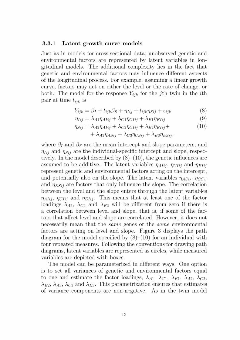
3.3.1 Latent growth curve models

Just as in models for cross-sectional data, unobserved genetic andenvironmental factors are represented by latent variables in lon-gitudinal models. The additional complexity lies in the fact thatgenetic and environmental factors may influence different aspectsof the longitudinal process. For example, assuming a linear growthcurve, factors may act on either the level or the rate of change, orboth. The model for the response Yijk for the jth twin in the ithpair at time tijk is

Yijk = βI + tijkβS + ηIij + tijkηSij + εijk (8)

ηIij = λA1ηAIij + λC1ηCIij + λE1ηEIij (9)

ηSij = λA2ηAIij + λC2ηCIij + λE2ηEIij+ (10)

+ λA3ηASij + λC3ηCSij + λE3ηESij,

where βI and βS are the mean intercept and slope parameters, andηIij and ηSij are the individual-specific intercept and slope, respec-tively. In the model described by (8)–(10), the genetic influences areassumed to be additive. The latent variables ηAIij, ηCIij and ηEIij

represent genetic and environmental factors acting on the intercept,and potentially also on the slope. The latent variables ηASij, ηCSij

and ηESij are factors that only influence the slope. The correlationbetween the level and the slope enters through the latent variablesηAIij, ηCIij and ηEIij. This means that at least one of the factorloadings λA2, λC2 and λE2 will be different from zero if there isa correlation between level and slope, that is, if some of the fac-tors that affect level and slope are correlated. However, it does notnecessarily mean that the same genes or the same environmentalfactors are acting on level and slope. Figure 3 displays the pathdiagram for the model specified by (8)–(10) for an individual withfour repeated measures. Following the conventions for drawing pathdiagrams, latent variables are represented as circles, while measuredvariables are depicted with boxes.

The model can be parameterized in different ways. One optionis to set all variances of genetic and environmental factors equalto one and estimate the factor loadings, λA1, λC1, λE1, λA2, λC2,λE2, λA3, λC3 and λE3. This parametrization ensures that estimatesof variance components are non-negative. As in the twin model

13

for cross-sectional data, we assume that many independent factorsare involved, i.e. that the latent variables representing genetic andenvironmental factors are independent and multivariate normallydistributed. We further assume that error terms are independentand normally distributed with mean zero and the same variance φ.

In longitudinal models for twin data, the trait value is usuallya linear function of the individual-specific growth variables (e.g.McArdle, 1986; Reynolds et al., 2002a,b). Neale and McArdle (2000)describe latent growth curve models for dynamic processes that arenonlinear in the individual-specific latent growth variables. As men-tioned in section 3.2, nonlinearity complicates model estimation.Neale and McArdle (2000) solve this by adapting a first-order lin-earization, which is described in section 4.1.

Y14Y11 Y12 Y13 Y21 Y22

ηI1 ηS1

ηAI1 ηCI1 ηCS1 ηES1

ηI2 ηS2

ηAI2

Y24Y23

ηEI2 ηCS2 ηES2

ρ=1

ηAS2

ρ=1 for MZρ=0.5 for DZ ρ=1

ρ=1 for MZρ=0.5 for DZ

11

λA2

λC1

11

λC2

λA1

ηEI1 ηAS1

λC3 λE3λA3

λE2

λE1

t11

t12

t13

t14

twin 1 twin 2

e14e13 e23e22e21 e24e12e11

ηCI2

Figure 3: Path diagram for a linear latent growth curve model for twins, includingadditive genetic (A), shared (C), and nonshared (E) environmental effects onintercept (ηI) and slope (ηS).

14

3.3.2 Linear latent variable models

A general formulation of the linear latent variable model (structuralequation model), which extends the twin model (8)–(10), can beexpressed as in Muthen and Muthen (1998–2004):

Yi = Λiηi + X1iβ + εi (11)

ηi = Bηi + X2iΓ + ζi. (12)

Model (11) is called the measurement model and has the same formas model (4), except that twin pairs are now the units of clusteringon the highest level, which we indicate by using the index i. Model(12) is called the structural model and specifies the structure forthe latent variables. As before, β denotes the vector of regressionparameters related to observed covariates X1i. B is a parametermatrix of slopes for regression of latent variables on other latentvariables and thus has zero diagonal elements. It is assumed that(I −B) is non-singular so that (I −B)−1 exists. Then (12) can besolved algebraically and written in reduced form with ηi only ap-pearing on the left-hand side. Γ is a parameter matrix for regressionof the latent variables on known covariates X2i, and ζi are vectorsof zero mean random errors. Inserting the reduced form expressionfor ηi obtained from (12) into the measurement model (11) givesthe reduced form model for Yi:

Yi = Λi(I−B)−1X2iΓ + X1iβ + Λi(I−B)−1ζi + εi.

The mean vector, µi, and the variance-covariance matrix, Σi, forYi are thus

µi = Λi(I−B)−1X2iΓ + X1iβ (13)

Σi = Λi(I−B)−1Ψi((I−B)−1)TΛTi + Φi, (14)

where Ψi is the variance-covariance matrix for the random errors ζi.The index i in Ψi indicates that the variance-covariance structureneed not be the same for all units. Φi is the variance-covariancematrix for the error terms εi. When the observed outcomes Yi areconditionally independent given the latent variables ηi, Φi will bediagonal. In the latent growth curve model (8)–(10), the parametersto be estimated are the factor loadings in B, the variance parameterin Φi, and the regression parameters in β.

15

3.3.3 Variance profiles

In behavioral genetics there is a specific interest in the trait varianceexpressed as a function of age, dissected into genetic and environ-mental components. For linear latent variable models, the variancecomponents profiles can be calculated from expression (14). Becausethe time points enter into the matrix Λi, the shape of the varianceprofiles are driven by the choice of growth curve model. As an il-lustration, consider the linear latent growth curve model specifiedby (8)-(10). In this model, the variance-covariance structure for theindividual-specific intercept and slope is

Var(ηIij) = λ2A1 + λ2

C1 + λ2E1

Var(ηSij) = λ2A2 + λ2

C2 + λ2E2 + λ2

A3 + λ2C3 + λ2

E3

Cov(ηIij, ηSij) = λA1λA2 + λC1λC2 + λE1λE2.

Based on these expressions, the variance of Yij at time t, V (t),can be calculated and decomposed into genetic and environmentalcomponents:

V (t) = VA(t) + VC(t) + VE(t) + φ

VA(t) = λ2A1 + 2tλA1λA2 + t2(λ2

A2 + λ2A3)

VC(t) = λ2C1 + 2tλC1λC2 + t2(λ2

C2 + λ2C3)

VE(t) = λ2E1 + 2tλE1λE2 + t2(λ2

E2 + λ2E3),

where φ is the variance of the error term. In the linear latent growthcurve model, V (t) is thus a function of t and t2, which restricts theestimated variance curves to be of some specific forms. Estimatedvariance component profiles based on results from fitting model (8)-(10) to the Symbol Digit test scores in SATSA have been plotted inFigure 4.

The inherent restrictions on the shape of the variance curves areproblematic, since the variance curves are the quantities of interestand presumably sensitive to the choice of growth curve model. InPaper I we investigate the ability of the random change point model(7) to capture the marginal trait variance as a function of age. In ananalysis of cognitive function based on SATSA data, we demonstratethat the random change point model captures the observed varianceprofile well, in contrast to the linear and the quadratic random

16

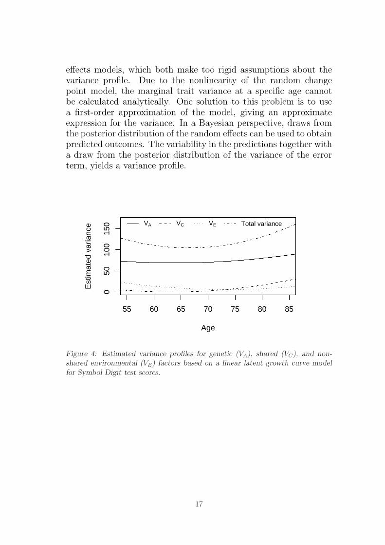
effects models, which both make too rigid assumptions about thevariance profile. Due to the nonlinearity of the random changepoint model, the marginal trait variance at a specific age cannotbe calculated analytically. One solution to this problem is to usea first-order approximation of the model, giving an approximateexpression for the variance. In a Bayesian perspective, draws fromthe posterior distribution of the random effects can be used to obtainpredicted outcomes. The variability in the predictions together witha draw from the posterior distribution of the variance of the errorterm, yields a variance profile.

55 60 65 70 75 80 85

050

100

150

Age

Est

imat

ed v

aria

nce VA VC VE Total variance

Figure 4: Estimated variance profiles for genetic (VA), shared (VC), and non-shared environmental (VE) factors based on a linear latent growth curve modelfor Symbol Digit test scores.

17

4 Likelihood inference

4.1 Maximum likelihood estimation

Maximum likelihood (ML) methods are widely used for fitting thetype of linear latent variable models described in section 3.3. MLestimators have many nice properties: they are consistent, asymp-totically unbiased, asymptotically normal and asymptotically effi-cient, i.e. no other consistent estimators can have a smaller asymp-totic variance. When Yi is multivariate normally distributed, as inthe linear latent variable models, ML is straightforward. For non-normally distributed Yi, however, exact ML is not always possibleand approximate methods have to be used. In Paper I, we evaluatethe performance of an approximate maximum likelihood procedurefor fitting the random change point model (7).

4.1.1 The likelihood

In latent variable models, the complete data from n units are (Y, η)with Y = (YT

1 , ...,YTn )T and η = (ηT

1 , ..., ηTn )T . Only Y is observed.

Letting θ denote variance parameters for η, and φ the varianceparameters for the error terms, the marginal density of Y is obtainedfrom

p(Y|X, β, θ, φ) =

∫p(Y|X, η, β, φ)p(η|θ)dη, (15)

where X denotes the covariate matrix associated with the fixed ef-fects parameters β. p(Y|X, β, θ, φ) is the marginal density of Y,p(Y|X, η, β, φ) is the conditional density of Y given the randomeffects η, and p(η|θ) is the marginal distribution of η.

4.1.2 Linear latent variable models

The integral in (15) can in some instances be expressed in closedform and evaluated analytically. When both p(Yi|Xi, β, θ, φ) andp(ηi|θ) are multivariate normal densities, the marginal distributionof Yi is multivariate normal. For models of the form (11)–(12),the mean vector, µi, and variance-covariance matrix, Σi, are givenby (13) and (14), respectively. Thus, estimates of β, θ, and φ are

18

obtained from maximizing the loglikelihood

`(β, θ, φ|Y) =n∑

i=1

(−1

2log |Σi| − 1

2(Yi − µi)

T Σ−1i (Yi − µi)

), (16)

where µi = µi(β) and Σi = Σi(θ, φ). In general, the likelihoodfunction (16) is a complicated nonlinear function of β, θ, and φ,and iterative numerical optimization procedures are necessary toobtain the maximum likelihood estimates.

Maximum likelihood estimators of variance-covariance parame-ters in latent variable models are expected to be biased downwards.To address this problem a so-called restricted or residual maximumlikelihood (REML) method can be used (Patterson and Thompson,1971). In this case, ML is not applied directly to the responsesYi but instead to linear functions of the responses AiYi, whereAi is chosen so that E(AiYi) = 0. In this way, the fixed effectsare ‘swept out’ from the model. In a Bayesian perspective, REMLcan be derived from integrating out β, that is, marginalizing withrespect to a flat prior density (e.g. Harville, 1977; Dempster et al.,1981). REML, unlike ML, produces unbiased estimators of varianceparameters in balanced study designs. However, the bias of ML es-timates will be important only if the number of units, n, is smallcompared to the number of fixed effects. In the models consideredin this thesis, the units of clustering are either twin pairs or repeatedmeasurements on individuals. The number of fixed effects is smallcompared to the number of units and REML and ML are expectedto give similar results.

4.1.3 Nonlinear latent variable models

Generalized linear random intercept models, i.e. special cases of(5), can also have closed-form likelihoods (e.g. Skrondal and Rabe-Hesketh, 2004). In general, however, the integral in (15) does nothave a closed-form expression. To make the numerical optimizationof the likelihood function tractable, different approximations havebeen proposed in the literature.

In Paper I, we consider the random change point model (7),which belongs to the family of nonlinear mixed models (6), for de-scribing repeated measurements on cognitive function in old age.

19

For the estimation of model parameters, we evaluate the first-orderlinearization method advocated by Beal and Sheiner (1982), whichis an approximate maximum likelihood approach. The idea is toapproximate the nonlinear model (6) with the first terms in a Tay-lor expansion around the expected value of the random effects, thatis, around ηj = 0. Retaining the first two terms in the expressiongives

Yj ≈ f j(Xj,0, β) + Fj(Xj,0, β, )ηj + εj, (17)

where Fj(Xj,0, β) is the matrix of first order partial derivatives off j(Xj, ηj, β) with respect to ηj, evaluated at ηj = 0. Expression(17) is linear in the random effects ηj, and a nonlinear function ofthe fixed effects, β. The important consequence of (17) is that themarginal mean and covariance of Yj may be specified readily as:

E(Yj) ≈ f j(Xj,0, β), (18)

Cov(Yj) ≈ Fj(Xj,0, β)ΨFTj (Xj,0, β) + φInj

, (19)

where Injis the nj × nj identity matrix, and Ψ is the covariance

matrix for ηj. If ηj and εj are normally distributed, it follows from(17) that the marginal distribution of Yj is approximately normalwith moments given by (18) and (19), and inference may be basedon standard asymptotic theory under the assumption that (17) is agood approximation.

A refinement of the first-order linearization method is the con-ditional first-order linearization of Lindstrom and Bates (1990).Here, the first-order Taylor expansion is evaluated at the condi-tional modes of ηj, that is, around the empirical Bayes estimatesηj. This procedure involves an additional computational burdensince it requires an alternating algorithm, but is expected to re-duce bias in parameter estimates from the approximation in (17).The difference between the first-order and the conditional first-orderanalyses will decrease as the number of observations per individualdecreases. The reason is that the empirical Bayes estimates, ηj,are ‘shrunk’ towards the mean value of zero, and the shrinkage isgreater when less data are available for each individual (Davidianand Giltinan, 1995, pp. 186–187).

There are several alternatives to the linearization methods de-scribed above for estimation of nonlinear mixed models. These in-clude Laplacian approximation, importance sampling, Monte Carlo

20

EM, and various quadrature rules, such as adaptive Gaussian quadra-ture (for a comparison of methods see Pinheiro and Bates, 1995).These alternative procedures may perform better than the lineariza-tion methods, but are in general computationally intensive.

4.2 Goodness-of-fit

Likelihood ratio tests of nested models and comparisons of AIC andBIC measures for non-nested models are commonly used for assess-ing goodness-of-fit of twin models to empirical data. The assessmentof genetic and environmental influences is usually based on standardlikelihood theory. However, the test of genetic and environmentalvariance components is in fact a nonstandard problem, correspond-ing to a test of a hypothesis on the boundary of the parameter space.In this section, the ideas underlying likelihood theory are reviewed,and the details of Paper III on the likelihood ratio test of variancecomponents are explained.

4.2.1 Asymptotic likelihood theory

Consider the log-likelihood function for some parameter vector θ =(θ1, ..., θH)T based on observed data Y, `(θ) = `(θ|Y). Asymptotictheory for the maximum likelihood estimator of θ, and tests of hy-potheses about θ, are based on a quadratic approximation to thelog-likelihood function:

`(θ) ≈ `(θ0) + STθ0

(θ − θ0)− 1

2(θ − θ0)

TIθ0(θ − θ0), (20)

where θ0 is the vector of true parameter values. Sθ0is the score func-

tion, that is, the vector of first order partial derivatives of `(θ) withrespect to the elements of θ, and Iθ0

is the (expected) Fisher infor-mation matrix, that is, minus the expectation of the Hessian matrix,evaluated at θ = θ0. Assuming regularity conditions, the score func-tion, Sθ0

, has a multivariate normal distribution with mean 0 andvariance-covariance matrix Iθ0

(e.g. Pawitan, 2001). This means

that the score function can be expressed as Sθ0= (I1/2

θ0)TZ, where

Z has a standard multivariate normal distribution with mean 0, andthe H ×H identity matrix as variance-covariance matrix.

21

The likelihood ratio test statistic, TLR, for the test of a null hy-pothesis H0 : θ = θ0 (meaning θh = θh0 for h = 1, ..., H) versusan alternative HA : θ 6= θ0 (meaning θh 6= θh0 for h = 1, ..., H) isdefined as

TLR = 2(supHA

`(θ)− `(θ0)).

To find the distribution of TLR, consider the parameter transforma-

tion υ = I1/2θ0

(θ − θ0). From expression (20) we then get

`(θ)− `(θ0) ≈ STθ0

(θ − θ0)− 1

2(θ − θ0)

TIθ0(θ − θ0)

= ZTI1/2θ0

(θ − θ0)− 1

2(θ − θ0)

TIθ0(θ − θ0)

= ZTυ − 1

2υTυ.

Under regularity conditions, ensuring that θ0 is an interior point ofthe parameter space, the estimator of υ that maximizes the expres-sion above is Z, and the likelihood ratio statistic becomes

TLR = 2 supHA

(ZTυ − 1

2υTυ) = ZTZ,

which has a χ2(H) distribution.

4.2.2 Tests of hypotheses on the boundary

The result that TLR asymptotically has a χ2 distribution does nothold if the null hypothesis places the parameter vector on the bound-ary of the parameter space, which violates the regularity conditions.One example that is common in twin analyses is the test of vari-ance components, where the null hypothesis value is zero and hencea boundary point.

The asymptotic distribution of TLR for tests where the null hy-pothesis value is a boundary point was examined already by Cher-noff in 1954. Self and Liang (1987) generalized the results of Cher-noff, and presented some special cases where the asymptotic distri-bution of the likelihood ratio statistic is obtained as a mixture ofchi-square distributions. An example where this distribution is not

22

a mixture of chi-square distributions was also given (Case 8 in Selfand Liang, 1987).

Sen and Silvapulle (2002) and Silvapulle and Sen (2005) give abroad description of constrained statistical inference, and refer tothe mixture of chi-square distributions as chi-bar squared distribu-tions. They discuss the computation of the chi-bar squared-weights,which in many practical situations may be difficult to compute ex-actly. In these situations, simulation techniques are needed. Inother situations, e.g. when sample sizes are small and asymptoticresults cannot be trusted, sampling methods may be preferable.

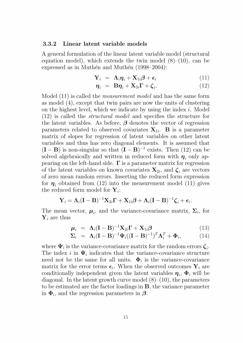
The asymptotic results for hypothesis testing under nonstandardconditions have been used in some fields of applications. For ex-ample, Stram and Lee (1994, 1995) addressed the problem of test-ing variance components in longitudinal random effects models. Intwin research, however, the fact that variance component testing isa nonstandard problem has been ignored. In Paper III, we describethe asymptotic distribution of the likelihood ratio statistic for testsinvolving up to two variance components.

γ

α

f2

f1

β

Υ2

Υ4Υ3

Υ1

υ1

υ2

Figure 5: Regions of the parameter space for υ = (υ1, υ2)T .

23

4.2.3 Likelihood ratio tests of variance components

Just as under standard conditions, the derivation of the asymptoticdistribution of TLR under nonstandard conditions is based on thequadratic approximation to the log-likelihood, and TLR is expressedin terms of Z and the new parameter set υ as previously described.In addition, the parameter space for θ is approximated with a conelocally around the null value θ0 (Self and Liang, 1987).

For a single variance component θ1, consider the test of H0 : θ1 =0 versus HA : θ1 > 0. Using the same terminology and notation asbefore, θ = θ1, Z = Z1, υ = υ1, and TLR = Z2

1I(Z1 > 0), whereZ1 ∼ N(0, 1) and I(·) is an indicator variable (Case 5 in Self andLiang, 1987). Hence, the asymptotic distribution of TLR is a 0.5:0.5mixture of χ2(0) (a distribution with a point mass at 0) and χ2(1).

For the test of two variance components, consider a model withparameters θ = (θ1, θ2)

T , and the test of H0 : θ1 = θ2 = 0 versusHA : θ1 > 0, θ2 > 0. In this case Z = (Z1, Z2)

T , where Z hasa bivariate standard normal distribution. The parameters θ are

transformed to υ = (υ1, υ2)T = I1/2

θ0(θ1, θ2)

T . By approximatingthe parameter space for θ with a cone locally around the null θ0 =(0, 0)T , the parameter space for υ can be described as in Figure 5,where the two vectors f1 and f2 are

f1 = I1/2θ0

(10

)and f2 = I1/2

θ0

(01

). (21)

The shaded region in Figure 5, Υ1, is the image of the region ofthe parameter space for θ = (θ1, θ2)

T where θ1 > 0 and θ2 > 0 (Case7 in Self and Liang, 1987). Observations in region Υ2 are projectedon to f2, observations in Υ3 are projected on to f1, and observationsin Υ4 are projected on to the origin, giving

TLR =

0 if (υ1, υ2) ∈ Υ4

Z22 if (υ1, υ2) ∈ Υ3

Z21 if (υ1, υ2) ∈ Υ2

Z21 + Z2

2 if (υ1, υ2) ∈ Υ1.

24

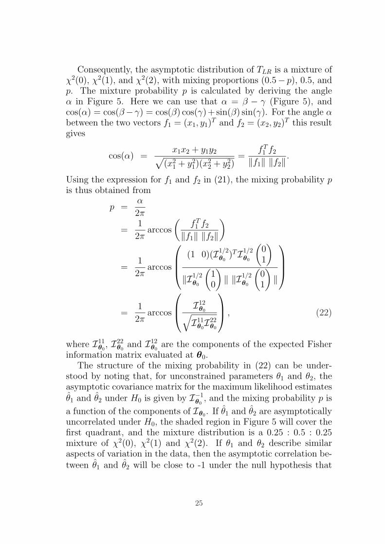
Consequently, the asymptotic distribution of TLR is a mixture ofχ2(0), χ2(1), and χ2(2), with mixing proportions (0.5− p), 0.5, andp. The mixture probability p is calculated by deriving the angleα in Figure 5. Here we can use that α = β − γ (Figure 5), andcos(α) = cos(β−γ) = cos(β) cos(γ)+ sin(β) sin(γ). For the angle αbetween the two vectors f1 = (x1, y1)

T and f2 = (x2, y2)T this result

gives

cos(α) =x1x2 + y1y2√

(x21 + y2

1)(x22 + y2

2)=

fT1 f2

‖f1‖ ‖f2‖ .

Using the expression for f1 and f2 in (21), the mixing probability pis thus obtained from

p =α

2π

=1

2πarccos

(fT

1 f2

‖f1‖ ‖f2‖)

=1

2πarccos

(1 0)(I1/2θ0

)TI1/2θ0

(01

)

‖I1/2θ0

(10

)‖ ‖I1/2

θ0

(01

)‖

=1

2πarccos

I12

θ0√I11

θ0I22

θ0

, (22)

where I11θ0

, I22θ0

and I12θ0

are the components of the expected Fisherinformation matrix evaluated at θ0.

The structure of the mixing probability in (22) can be under-stood by noting that, for unconstrained parameters θ1 and θ2, theasymptotic covariance matrix for the maximum likelihood estimatesθ1 and θ2 under H0 is given by I−1

θ0, and the mixing probability p is

a function of the components of Iθ0. If θ1 and θ2 are asymptotically

uncorrelated under H0, the shaded region in Figure 5 will cover thefirst quadrant, and the mixture distribution is a 0.25 : 0.5 : 0.25mixture of χ2(0), χ2(1) and χ2(2). If θ1 and θ2 describe similaraspects of variation in the data, then the asymptotic correlation be-tween θ1 and θ2 will be close to -1 under the null hypothesis that

25

θ1 and θ2 are both equal to zero, and the ratio I12θ0

/√I11

θ0I22

θ0will be

close to 1. In this case, the mixing probability p obtained from (22)is small, which is expected: If θ1 and θ2 capture similar aspects ofvariation, we do not expect θ1 and θ2 to both be positive at the sametime if the true values of θ1 and θ2 are zero. Hence, the contributionof χ2(2) is expected to be small in this case.

The p-value for a test of two parameters on the boundary from anobserved likelihood ratio statistic value tLR based on the (0.5− p) :0.5 : p mixture of χ2(0), χ2(1) and χ2(2), is easily obtained from

(0.5− p) · p0(tLR) + 0.5 · p1(tLR) + p · p2(tLR),

where p is the mixture probability given by expression (22), andps(tLR) denotes the p-value for an observed test statistic tLR basedon the χ2(s) distribution.

4.2.4 Likelihood ratio tests of nested twin models

According to the results from the previous section, the p-value ob-tained from χ2(1) in a likelihood ratio test of one variance compo-nent should be divided by two to yield a correct inference. Theprocedure does not depend on the model or which variance compo-nent that is tested.

For a test of two variance components, the Fisher informationmatrix has to be calculated to obtain the correct reference distri-bution. Consider a twin model within the family of linear latentvariable models, with likelihood given by (16). For simplicity, weonly consider the variance component parameters θ = (θ1, ..., θH),and write Σi = Σi(θ), and `(θ) = `(θ|Y). The derivative of `(θ)with respect to θh (h = 1, ..., H) can be obtained using the followinggeneral results for the differentiation of matrix expressions:

∂Σ−1

∂θh= −Σ−1 ∂Σ

∂θhΣ−1 (23)

∂

∂θhlog |Σ| = tr

(Σ−1 ∂Σ

∂θh

), (24)

where tr() denotes the trace (Searle et al., 1992). Using (23) and(24), the first order partial derivative of `(θ) in (16) with respect to

26

θh can be expressed as

∂`(θ)∂θh

=n∑

i=1

(−1

2tr

(Σ−1

i

∂Σi

∂θh

)+

12(Yi − µi)

TΣ−1i

∂Σi

∂θhΣ−1

i (Yi − µi))

=n∑

i=1

(12tr

(−Σ−1i Σi(h) + Σ−1

i Σi(h)Σ−1i (Yi − µi)(Yi − µi)

T))

, (25)

where Σi(h) = ∂Σi

∂θh. The second equality is obtained by noting that

(Yi − µi)TA(Yi − µi) = tr(A(Yi − µi)(Yi − µi)

T ) for any non-stochastic matrix A. The components of the Hessian of `(θ), i.e.the second order partial derivatives, are obtained by again using thegeneral derivation rule (23) on expression (25). The expected Fisherinformation matrix I(θ) is obtained as minus the expectation of theHessian matrix. From E((Yi − µi)(Yi − µi)

T ) = Σi we obtain

Ihk(θ) = −E

(∂2`(θ)

∂θh∂θk

)=

n∑i=1

(1

2tr

(Σ−1

i Σi(h)Σ−1i Σi(k)

)). (26)

For models such as the longitudinal twin model for unbalanced datadescribed in section 3.3, Σ−1

i , Σi(h) and Σi(k) are different for alltwin pairs. On the other hand, for twin models where the variance-covariance structure only depends on zygosity there are only twovariance-covariance matrices, which we denote ΣMZ and ΣDZ . Inthis case, with data on nMZ MZ twin pairs and nDZ DZ twin pairs,expression (26) becomes

Ihk(θ) =nMZ

2tr

(Σ−1

MZΣMZ(h)Σ−1MZΣMZ(k)

)+

+nDZ

2tr

(Σ−1

DZΣDZ(h)Σ−1DZΣDZ(k)

),

(27)

where ΣMZ(h) = ∂ΣMZ

∂θhand ΣDZ(h) = ∂ΣDZ

∂θh.

Consider a test of two variance component parameters, say θ1and θ2, being components of the vector of variance-covariance pa-rameters, θ, describing ΣMZ and ΣDZ . The mixing probability forthe asymptotic distribution of the likelihood ratio statistic for thetest of H0 : θ1 = 0, θ2 = 0 versus HA : θ1 > 0, θ2 > 0 can be obtainedby first calculating I(θ)−1. We then invert the 2 × 2 submatrix ofI(θ)−1 corresponding to θ1 and θ2. The terms I11

θ0and I22

θ0in ex-

pression (22) are the diagonal elements, and I12θ0

the off-diagonalelement, of this matrix evaluated under H0.

27

In Paper III, we derive the mixture probability for the likelihoodratio test of the E model, only including individual-specific environ-mental effects, against the ACE model (2). We provide a formulafor the mixing probability p as a function of the ratio r = nMZ

nDZ, and

show that p ≈ 0.05 is a good approximation in all realistic situa-tions. The 0.45 : 0.5 : 0.05 mixture of χ2(0), χ2(1), and χ2(2) isfar from the χ2(2), which is commonly used as reference distribu-tion for this test. The small contribution of χ2(2) can be intuitivelyunderstood by noting that the genetic and environmental variancecomponents in the ACE model, λ2

A and λ2C , both capture familial

correlation. Hence, there is a very strong negative asymptotic corre-lation between the estimates of λ2

A and λ2C under the E model of no

familial correlation. Consequently, if there is no familial correlationit rarely happens that both estimates of λ2

A and λ2C are found to be

positive at the same time, and there is little contribution from theχ2(2) distribution.

4.2.5 Model selection based on relative fit criteria

Twin analyses are often of an hypothesis-generating nature. Sev-eral models are tried out and their relative fit to the available datais assessed. If inference is taken from the perspective that we arecomparing several working models on equal footing, not necessar-ily containing the true model, alternatives to the likelihood ratiotest are needed. One such overall model fit measure is the Akaikeinformation criterion (AIC), defined as

AIC = −2` + 2r,

where ` is the log-likelihood and r is the number of free modelparameters (Akaike, 1987). The first term in AIC can be interpretedas a measure of data fit and the second term as a penalty. Inthis formulation, small values of the AIC are preferable. The AIChas the advantage of also enabling comparisons of goodness-of-fitof non-nested models. An alternative to the AIC is the Bayesianinformation criterion (BIC), defined as

BIC = −2` + r log(N),

where N is the number of observations (Schwarz, 1978). Manyvariants of the AIC and the BIC measures exist (e.g. Burnham and

28

Anderson, 2002).Unfortunately, the problems for likelihood ratio tests of param-

eters on the boundary of the parameter space also affects the AICand the BIC. In addition, use of the AIC and the BIC in latentvariable models is not straightforward because it is not clear howthe number of degrees of freedom (effective number of parameters),should be determined. Hodges and Sargent (2001), Burnham andAnderson (2002) and Vaida and Blanchard (2005) argue that thedegrees of freedom lie somewhere between the number of model pa-rameters (excluding the latent variables) and the sum of the numberof model parameters and the number of realizations of the latentvariables. An additional difficulty with the application of BIC isthat the number of observations N must be specified, which is notstraightforward in latent variable modelling (Skrondal and Rabe-Hesketh, 2004, pp. 264–265).

29

5 Bayesian inference

An alternative to likelihood-based inference is to view the problemin a Bayesian perspective. In Bayesian analysis of hierarchical (ran-dom effects) models, Markov chain Monte Carlo (MCMC) methods,especially the Gibbs sampler, have been shown to be useful (e.g.Gelfand and Smith, 1990). In Paper I, we use a Gibbs sampler formodel estimation of the random change point model (7).

5.1 Three-stage hierarchical models

In the Bayesian analysis we make a conceptual shift and treat themodel parameters β (for fixed effects), θ (for random effects), andφ (for error terms) as random, while the data Y = (YT

1 , ...,YTn )T

(from a sample of n individuals) are treated as fixed. Writing theindividual effects as the sum of fixed effects and random effects, wehave bj = β + ηj for the jth individual, and b = (bT

1 , ...,bTn )T .

The model can be specified as a three-stage hierarchical model, byspecifying p(Y|X,b, φ), the conditional likelihood for the data givenb and φ (stage 1), p(b|β, θ), the joint prior for the random effects(stage 2), and p(β, θ, φ), the joint (hyper)prior distributions for themodel parameters (stage 3). The joint posterior distribution of theunknowns in the three-stage hierarchical model is obtained from

p(β,b, θ, φ|Y,X) ∝ p(Y|X,b, φ)p(b|β, θ)p(β, θ, φ). (28)

The models specified in stage 1 and stage 2 are the same as the onesspecified within the likelihood framework. In addition, we now alsospecify prior distributions for the model parameters β, θ, and φ.

In the hierarchical change point model (7), the parameters areβ = (β0, β1, β2, β3), θ is the vector of parameters in Ψ, which is thevariance-covariance matrix for the random effects, and φ = φ is thevariance of the error terms. We use conjugate priors for the modelparameters, which means that the posterior distributions follow thesame parametric form as the prior distributions. This is convenientin that the posterior distributions follow a known parametric form.In the most general specification, we use a multivariate normal dis-tribution as prior for β, an inverse-Wishart distribution as prior for

30

Ψ and an inverse-gamma distribution as prior for φ. The inverse-gamma(ε, ε), with ε set to a low value, is a typical choice of priordistribution for independent variance components, in an attempt atnoninformativeness within the conditional conjugate family. How-ever, the limit of ε → 0 results in an improper posterior density, andthus ε must be set to a reasonable value. For a general discussionof alternative prior distributions for variance components, refer toGelman (2005).

Marginal posterior distributions for the parameters β, θ, andφ can be obtained by integrating expression (28) over b. Themulti-dimensional integration required for explicit calculation of themarginal distributions may be prohibitive, in which case sampling-based procedures may be useful. One such procedure is Markovchain Monte Carlo simulation, which involves the construction andthe simulation of a Markov chain that has the posterior distribu-tion of interest as the stationary distribution. After deleting the firstpart of realizations of the Markov chain (the burn-in) to remove anyeffects of the choice of starting points, the posterior distribution isobtained from the simulated Markov chain.

5.2 MCMC for the hierarchical change point model

One way of constructing Markov chains is by the Gibbs sampler(e.g. Geman and Geman, 1984; Gelfand and Smith, 1990), involv-ing sampling from the full conditional distributions of all unknowns.The implementation of the Gibbs sampler thus relies on the abil-ity to sample from the relevant conditional distributions, which isstraightforward when the necessary full conditionals are explicitlyspecified. Due to the nonlinearity of the regression function in thehierarchical change point model, the full conditional density of eachbj, given the remaining parameters and the data, cannot be cal-culated explicitly. The conditional density of bj may, however, bewritten up to a proportionality constant. To overcome this problema Metropolis algorithm can be used within the Gibbs sampler. TheMetropolis algorithm is an adaption of a random walk that uses anacceptance/rejection rule to converge to the specified target distri-bution. It often starts with an adapting phase where the Metropolisjumps are tuned to get the acceptance rates desired (e.g. Davidian

31

and Giltinan, 1995).Just as in the context of maximum likelihood, it is desirable that

model parameters correspond approximately to contrasting featuresof the data. In the Bayesian analysis of the hierarchical changepoint model in Paper I, the stage 1 model in the hierarchy is thesame as in (7). This parametrization is useful for distinguishingbetween the slope parameters in the first and the second phase.However, some of the model parameters are still highly correlated,and long Markov chains are needed to reach convergence. Otherparameterizations, such as the one adapted by Lange et al. (1992),could improve convergence.

In the implementation of the Gibbs sampler, questions arise con-cerning how long and how many Markov chains should be run.There are no clear answers to these questions. However, runningmany short chains, motivated by a desire to obtain independentsamples from the stationary distribution, seems to be misguidedunless there is some special reason for needing independent samples(Gilks et al., 1996). In the application of the Gibbs sampler for thehierarchical change point model, we run two parallel chains, aimingto obtain as long chains as possible and still being able to assess therobustness to the choice of starting point.

There exist many methods for monitoring convergence of simu-lated Markov chains, for an overview see Brooks and Roberts (1998).In our application of the Gibbs sampler, we use the diagnostic cri-terion proposed by Geweke (1992) and assess convergence of eachMarkov chain separately. Geweke’s diagnostic criterion correspondsto a test for equality of the means in the first and the last partof a Markov chain. If the samples are drawn from the stationarydistribution of the chain, the two means are equal and Geweke’sstatistic has an asymptotically standard normal distribution. Thetest statistic is a standard Z-score: the difference between the twosample means divided by its estimated standard error.

32

6 Dropout from longitudinal twin studies

Loss to follow-up (dropout) of study participants, and nonresponsein general, can potentially bias results of statistical analyses. Theliterature on dropout from longitudinal studies is rich (e.g. Laird,1988; Diggle and Kenward, 1994). The consequences of nonresponsein twin studies has also been studied, but there is still confusionabout whether it is possible to say in which direction genetic andenvironmental variance component estimates will be biased. Mathe-matical derivations, as well as simulations, have shown that selection(nonresponse) reduces the size of within-pair correlations (Martinand Wilson, 1982; Neale et al., 1989). These earlier results clearlyshow that nonresponse may bias heritability estimates which relyon comparisons of MZ and DZ correlations. The effect of nonre-sponse on estimates of variance components in behavioral-geneticanalyses was studied in a set of simulations by Taylor (2004), sug-gesting that nonresponse primarily serves to attenuate the effect ofshared environment and inflate estimates of nonshared environmentand additive genetic effects. The aim of Paper II is to give a bal-anced picture of the problem and show that the magnitude and thedirection of the bias in variance component estimates depends onthe underlying nonresponse mechanism.

6.1 Missing value mechanisms

Little and Rubin (2002) describe a hierarchy that can be used fordistinguishing between different types of missing value mechanisms.To fix ideas, let Y denote the complete data matrix, Yobs the ob-served part, and Ymis the missing part, so that Y = (Yobs,Ymis).Let R be a matrix of indicator variables with elements equal tozero or one depending on whether the corresponding elements of Yare missing or observed. A probability model for the missing valuemechanism defines the probability distribution of R conditional onY = (Yobs,Ymis). Little and Rubin say that missing values are

• Missing completely at random (MCAR) if R is independent ofboth Yobs and Ymis

• Missing at random (MAR) if R is independent of Ymis

33

• Informative if R is dependent of Ymis.

Thus, despite the name, MAR does not suggest that the missing val-ues are a simple random sample of all values; it only requires thatthe missing values behave like a random sample of all values withinsubclasses defined by the observed data. For likelihood-based infer-ence, the important distinction is between random and informativemissing value mechanisms. To see this, consider the probability dis-tribution of the observed data. If some of the data are missing the‘observed data’ truly consist not only of Yobs but also of R and theprobability distribution of the observed data is given by

p(R,Yobs|θ, ξ) =

∫p(R,Y|θ, ξ)dYmis

=

∫p(R|Y, ξ)p(Y|θ)dYmis,

where θ are the model parameters for Y, and ξ are the modelparameters for R. When missing values are MAR, the probabilitydistribution of the observed data simplifies to

p(R,Yobs|θ, ξ) = p(R|Yobs, ξ)

∫p(Y|θ)dYmis

= p(R|Yobs, ξ)p(Yobs|θ).

Taking logarithms in the expression above, the log-likelihood func-tion is

`(θ, ξ|R,Y) = `(ξ|R,Yobs) + `(θ|Yobs),

which is maximized by separate maximization of the two terms onthe right-hand side. The first term contains no information aboutthe distribution of Yobs, and can be ignored for the purpose of mak-ing inferences about Yobs. This requires that the measurement pa-rameters, θ, and the missing value mechanism parameters, ξ, arevariation independent, or ‘distinct’ (Little and Rubin, 2002). Thismeans that no group of parameter values for θ restricts the possiblerange of values of any parameters in ξ, and vice versa. If missingvalues are MAR and θ and ξ are distinct, the missing value mech-anism is said to be ignorable, and if not, the missing value mecha-nism is non-ignorable, or informative (Little and Rubin, 2002). Note

34

that θ refers to the parameters of the model for the complete dataY = (Yobs,Ymis), not the parameters for the distribution of Yobs

alone.

6.2 Ignorable dropout

If the missing value mechanism underlying dropout is ignorable, es-timation of θ can be based on the likelihood ignoring the missingvalue mechanism, `(θ|Yobs). This is sometimes referred to as fullinformation maximum likelihood (FIML), or raw maximum likeli-hood (Lange et al., 1976; Arbuckle, 1996), and is usually the basisfor model estimation based on incomplete twin data. For the linearlatent variable models described in section 3.3, Yobs

i simply replacesthe complete data Yi in the log-likelihood given by (16).

Missing data can alternatively be handled by multiple imputationmethods (e.g. Rubin, 1987; Schafer, 1997). Multiple imputation isbased on the idea of imputing values that are missing, based on animputation model for missing values given the observed data, andaveraging over multiple imputations. This procedure provides con-sistent estimates as long as the missing data mechanism is ignorable.The observed likelihood method can be seen as a multiple imputa-tion approach where infinitely many imputations are performed.The advantage with multiple imputation is that it can handle bothmissing covariates and missing responses.

6.3 Modelling the dropout process

If the missing value mechanism is non-ignorable, the proceduresdescribed above may yield biased parameter estimates. To accom-modate a non-ignorable missing value mechanism, joint models forthe longitudinal and the missingness processes can be formulated.

In the ‘selection model’ approach (e.g. Little, 1995), the depen-dence of the missingness process on the unobserved response is ex-plicitly modeled. In other words, the joint distribution of Y and Ris factorized as the marginal distribution of Y and the conditionaldistribution of R given Y, that is, p(R,Y) = p(Y)p(R|Y). Inthe setting of dropout from a longitudinal study, Diggle and Ken-ward (1994) model the dropout at each time-point (given that it

35

has not yet occurred) using a logistic regression model with previ-ous responses and the contemporaneous response as covariates. Ifdropout occurs, the contemporaneous response is not observed butcan be represented by a latent variable, and the likelihood is thejoint likelihood of the response and dropout status after integratingout the latent variable.

The joint distribution of Y and R can alteratively be factor-ized in terms of the marginal distribution of R and the conditionaldistribution of Y given R, that is, p(R,Y) = p(R)p(Y|R). Thesemodels are referred to as pattern-mixture models, and are especiallyuseful when the focus is on Y conditional on missing value patterns(e.g. Little, 1993; Hogan and Laird, 1997).

Yet another approach for incorporating informative dropout, andnonresponse in general, is to adapt a random effects model. Here,an individual’s propensity to drop out depends on unobserved vari-ables, that is, on random effects. Postulating the latent variablesη = (ηR, ηY ), the joint distribution of Y, R and η is

p(R,Y, η) = p(Y|ηY )p(R|ηR)p(η). (29)

The dependence between R and Y is a by-product of a dependencebetween the latent variables ηR and ηY .

In Paper II, we formulate a model for twin data with informativenonresponse, which can be expressed as in (29). The factors ηR andηY are decomposed into genetic and environmental factors, and thefactors underlying ηR and ηY are allowed to be correlated. In asimulation study, we assess the bias in FIML estimates of the geneticand environmental variance components for different scenarios. Wedemonstrate that the bias does not only depend on the value of thecorrelation between ηR and ηY , but also on the mechanism givingrise to the correlation.

In analyses of cognitive function from SATSA, based on measure-ments at occasions 13 years apart, the estimated genetic variancebased on FIML decreases dramatically. The decrease is potentiallypartly explained by the dropout of study participants. However, oursimulations suggest that even with a highly informative dropoutmechanism it is unlikely that the dramatic decrease solely is at-tributable to the dropout. This result supports the hypothesis thatgenetic influences on some cognitive abilities decrease with age in

36

late life.Modelling informative dropout is clearly associated with identifi-

ability problems, since it is impossible to verify the model assump-tions based on empirical data. On the other hand, relying on theassumption of ignorable dropout, which is untestable as well, mayyield biased estimates. It is therefore recommendable that differentscenarios for the dropout mechanism are considered, to get an ideaof the potential effect of the dropout mechanism. Molenberghs et al.(2003) argue that the treatment of incomplete data should be em-bedded within a sensitivity analysis, and present several modellingstrategies.

6.4 Dropout due to death

Standard approaches for handling missing data assume that miss-ing values hide true values, and estimation of parameters are per-formed by integrating over, or imputing, missing values. Trunca-tion of follow-up data due to death is conceptually different fromdropout where the individual is still alive. For most outcomes it isnot reasonable to think of missing values after death, since they arecounterfactual and poorly defined. The value is not ‘missing’ be-cause an existing value is unobserved, but because no value exists.Within the framework of marginal models, models conditional onbeing alive have been described (e.g. Dufouil et al., 2004; Kurlandand Heagerty, 2005). The methods proposed make a distinction be-tween dropout and truncation by death in analyses based on inverseprobability of censoring-weighted generalized estimating equations(Robins et al., 1995). How truncation by death should be accountedfor within the framework of latent variable models for modelling lon-gitudinal twin data, remains to be explored.

37

7 Discussion

Longitudinal family studies provide important information for ex-ploring sources of variation in human traits. To fully make use of theinformation from such studies, statistical tools have to be developedand refined. This thesis contributes to this process by addressingvarious questions related to the statistical analysis of longitudinaltwin data.

Latent growth curve models commonly used for analysing lon-gitudinal twin data implicitly impose restrictions on the variance-covariance structure. This is problematic, since a central goal oflongitudinal twin analyses is to decompose trait variance into ge-netic and environmental variance components as functions of age.Hence, it is desirable that growth curve models are flexible in thisrespect. In Paper I, we describe a random change point model forcognitive function in old age, and demonstrate its ability to capturetrait variance as a function of age. The extension of the randomchange point model to incorporate the dependence within twin pairsis a topic for future work.

In models for incomplete twin data, it is usually assumed that themissing data mechanism is ignorable. In Paper II, we investigatehow estimates of genetic and environmental variance componentsmay be affected if the ignorability assumption is violated. Unfortu-nately, there is no simple answer to this question. It all depends onhow the factors driving the nonresponse are related to the factorsinfluencing the trait. Relaxing the assumption that dropout fromlongitudinal twin studies is ignorable remains a challenge for futureresearch.

In studies of aging, joint modelling of longitudinal data and sur-vival seems appropriate. The literature on such joint models isextensive. An interesting example is the model of Jacqmin-Gaddaet al. (2005), including a random change point model for repeatedmeasures on cognitive function and a survival model for age at onsetof dementia. These model extensions necessitate additional modelassumptions, which will most likely be impossible to test. Hence,sensitivity assessments, providing bounds on parameters of interestfor different scenarios for the missing data mechanism, will play animportant role.

38

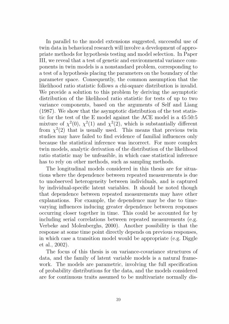
In parallel to the model extensions suggested, successful use oftwin data in behavioral research will involve a development of appro-priate methods for hypothesis testing and model selection. In PaperIII, we reveal that a test of genetic and environmental variance com-ponents in twin models is a nonstandard problem, corresponding toa test of a hypothesis placing the parameters on the boundary of theparameter space. Consequently, the common assumption that thelikelihood ratio statistic follows a chi-square distribution is invalid.We provide a solution to this problem by deriving the asymptoticdistribution of the likelihood ratio statistic for tests of up to twovariance components, based on the arguments of Self and Liang(1987). We show that the asymptotic distribution of the test statis-tic for the test of the E model against the ACE model is a 45:50:5mixture of χ2(0), χ2(1) and χ2(2), which is substantially differentfrom χ2(2) that is usually used. This means that previous twinstudies may have failed to find evidence of familial influences onlybecause the statistical inference was incorrect. For more complextwin models, analytic derivation of the distribution of the likelihoodratio statistic may be unfeasible, in which case statistical inferencehas to rely on other methods, such as sampling methods.

The longitudinal models considered in this thesis are for situa-tions where the dependence between repeated measurements is dueto unobserved heterogeneity between individuals, and is capturedby individual-specific latent variables. It should be noted thoughthat dependence between repeated measurements may have otherexplanations. For example, the dependence may be due to time-varying influences inducing greater dependence between responsesoccurring closer together in time. This could be accounted for byincluding serial correlations between repeated measurements (e.g.Verbeke and Molenberghs, 2000). Another possibility is that theresponse at some time point directly depends on previous responses,in which case a transition model would be appropriate (e.g. Diggleet al., 2002).

The focus of this thesis is on variance-covariance structures ofdata, and the family of latent variable models is a natural frame-work. The models are parametric, involving the full specificationof probability distributions for the data, and the models consideredare for continuous traits assumed to be multivariate normally dis-

39

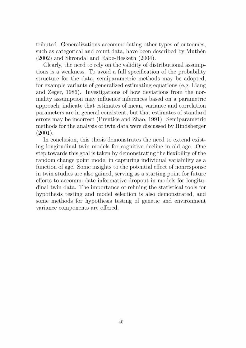
tributed. Generalizations accommodating other types of outcomes,such as categorical and count data, have been described by Muthen(2002) and Skrondal and Rabe-Hesketh (2004).

Clearly, the need to rely on the validity of distributional assump-tions is a weakness. To avoid a full specification of the probabilitystructure for the data, semiparametric methods may be adopted,for example variants of generalized estimating equations (e.g. Liangand Zeger, 1986). Investigations of how deviations from the nor-mality assumption may influence inferences based on a parametricapproach, indicate that estimates of mean, variance and correlationparameters are in general consistent, but that estimates of standarderrors may be incorrect (Prentice and Zhao, 1991). Semiparametricmethods for the analysis of twin data were discussed by Hindsberger(2001).

In conclusion, this thesis demonstrates the need to extend exist-ing longitudinal twin models for cognitive decline in old age. Onestep towards this goal is taken by demonstrating the flexibility of therandom change point model in capturing individual variability as afunction of age. Some insights to the potential effect of nonresponsein twin studies are also gained, serving as a starting point for futureefforts to accommodate informative dropout in models for longitu-dinal twin data. The importance of refining the statistical tools forhypothesis testing and model selection is also demonstrated, andsome methods for hypothesis testing of genetic and environmentvariance components are offered.

40

8 Svensk sammanfattning

Longitudinella studier av tvillingar tillfor viktig information i sokan-det efter en forklaring till hur arv och miljo paverkar manskligaegenskaper och hur denna paverkan forandras med aldern. I stati-stiska modeller for upprepade matningar pa tvillingar representerasgener och miljofaktorer som inte ar observerade av latenta variablermed en specificerad sannolikhetsfordelning. Pa sa satt kan varia-tionen i en egenskap hos olika individer delas upp i komponentersom forklaras av gener och miljofaktorer. Varianskomponenternakan sedan beskrivas som en funktion av alder.

Denna avhandling ar en bred syntes av statistisk modelleringav longitudinella tvillingdata och utvecklar denna genom att (i)utvardera en tva-fas-modell for modellering av variation som enfunktion av alder baserat pa longitudinella data, (ii) undersokahur skattningar av varianskomponenter paverkas av bortfall frantvillingstudier, och (iii) presentera en metod for hypotestest av vari-anskomponenter. Statistisk metodik illustreras med analyser av em-piriska data pa kognitiv formaga fran en longitudinell studie kringaldrande (the Swedish Adoption/Twin Study of Aging, SATSA).

De ovan namnda bidragen aterfinns i tre artiklar som en delav avhandlingen. I den inledande delen av avhandlingen beskrivsideerna bakom statistisk modellering av tvillingdata och longitudi-nella data, och hur de knyts samman i modellering av longitudinellatvillingdata. Likelihood-baserad inferens kontrasteras med Bayesi-ansk inferens, och fragestallningar kring bortfall av deltagare i tvil-lingstudier diskuteras. Detaljerna bakom resultaten i artiklarnabeskrivs och amnen for framtida forskning pekas ut.

I artikel I jamfors olika modeller for att beskriva individers pro-filer fran upprepade matningar over tid. Vi formulerar en tva-fas-modell dar aldern vid overgang fran den forsta till den andra fasentillats vara olika for olika individer. Modellen ar icke-linjar i delatenta variabler som beskriver en individs profil over tid, vilketkomplicerar skattning av modellparametrar. En approximativ max-imum likelihood-metod som ar baserad pa en linjarisering av mod-ellen utvarderas och jamfors med en Bayesiansk metod som ar base-rad pa Markov chain Monte Carlo simulering. Vi visar att tva-fas-modellen, till skillnad fran den linjara och den kvadratiska modellen

41

som ofta anvands for att beskriva en individs forandring over tid,ar flexibel i att beskriva variationen som en funktion av alder.

I artikel II undersoks hur skattningar av varianskomponenterpaverkas nar tvillingdata ar ofullstandiga, t.ex. pa grund av bortfallav deltagare i longitudinella studier. Den metod som ofta anvandsfor att anpassa modeller till ofullstandiga tvillingdata ar baserad paett antagande om icke-informativt bortfall, d.v.s. att bortfallsmekan-ismen helt kan forklaras av observerade data. Vi formulerar en mod-ell for tvillingdata med informativt bortfall och visar att bortfall-ets paverkan helt beror pa hur faktorerna som styr bortfallsmekan-ismen hanger ihop med de faktorer som influerar egenskapen i fraga.Matningar av kognitiv formaga fran SATSA, gjorda med 13 arsmellanrum, analyseras och en markant nedgang i skattad genetiskvarians observeras. Baserat pa en simuleringsstudie utifran ett an-tal olika hypoteser om den underliggande bortfallsmekanismen, drarvi slutsatsen att nedgangen inte helt kan forklaras av borfallet avdeltagare i studien.

I artikel III presenteras en metod for hypotesprovning av var-ianskomponenter i statistiska modeller for familjedata. Eftersomvarianser ar icke-negativa placerar nollhypotesen parametrarna paranden av parameterrymden. Det medfor att standardresultat inommaximum-likelihood-teori som brukar anvandas ger felaktiga resul-tat. Som losning till detta harleder vi den asymptotiska fordelnin-gen for likelihood-kvot-statistikan for test av varianskomponenternai klassiska tvillingmodeller. Resultatet ar en mix av chi-tva-fordel-ningar. Fordelningen har storre sannolikhetsmassa for sma vardenpa likelihood-kvot-statistikan an den chi-tva-fordelning som brukaranvandas. Det betyder att tidigare tvillingstudier kan ha misslyck-ats att pavisa genetiska effekter endast pa grund av att fel sanno-likhetsfordelning har anvants.

42

References

Akaike, H. (1987). Factor analysis and AIC. Psychometrika, 52, 317–332.

Arbuckle, J. L. (1996). Full information estimation in the presenceof incomplete data. In G. A. Marcoulides and R. E. Schumacker(Eds.), Advanced Structural Equation Modeling (pp. 243–277).Mahwah: Lawrence Erlbaum Associates.

Bacon, D. W. and Watts, D. G. (1971). Estimating the transitionbetween two intersecting straight lines. Biometrika, 58, 525–534.

Beal, S. L. and Sheiner, L. B. (1982). Estimating population kinet-ics. CRC Critical Reviews in Biomedical Engineering, 8, 195–222.

Bollen, K. A. (1989). Structural Equations with Latent Variables.New York: Wiley.

Breslow, N. E. and Clayton, D. G. (1993). Approximate inferencein generalized linear mixed models. Journal of the American Sta-tistical Association, 88, 9–25.

Brooks, S. P. and Roberts, G. O. (1998). Convergence assessmenttechniques for Markov chain Monte Carlo. Statistics and Comput-ing, 8, 319–335.

Burnham, K. P. and Anderson, D. R. (2002). Model Selectionand Multimodel Inference: A Practical Information-Theoretic Ap-proach (2nd ed.). New York: Springer.

Chernoff, H. (1954). On the distribution of the likelihood ratio. TheAnnals of Mathematical Statistics, 25, 573–578.

Davidian, M. and Giltinan, D. M. (1995). Nonlinear Models for Re-peated Measurement Data. Boca Raton: Chapman & Hall/CRC.

Dempster, A. P., Rubin, D. B. and Tsutakawa, R. K. (1981). Esti-mation in covariance components models. Journal of the AmericanStatistical Association, 76, 341–353.

Diggle, P. and Kenward, M. G. (1994). Informative drop-out inlongitudinal data analysis. Applied Statistics, 43, 49–93.

43

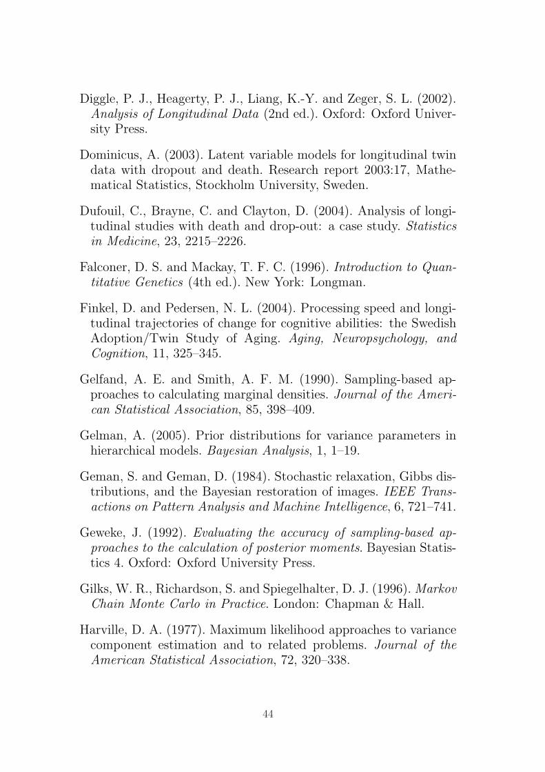
Diggle, P. J., Heagerty, P. J., Liang, K.-Y. and Zeger, S. L. (2002).Analysis of Longitudinal Data (2nd ed.). Oxford: Oxford Univer-sity Press.

Dominicus, A. (2003). Latent variable models for longitudinal twindata with dropout and death. Research report 2003:17, Mathe-matical Statistics, Stockholm University, Sweden.

Dufouil, C., Brayne, C. and Clayton, D. (2004). Analysis of longi-tudinal studies with death and drop-out: a case study. Statisticsin Medicine, 23, 2215–2226.

Falconer, D. S. and Mackay, T. F. C. (1996). Introduction to Quan-titative Genetics (4th ed.). New York: Longman.

Finkel, D. and Pedersen, N. L. (2004). Processing speed and longi-tudinal trajectories of change for cognitive abilities: the SwedishAdoption/Twin Study of Aging. Aging, Neuropsychology, andCognition, 11, 325–345.

Gelfand, A. E. and Smith, A. F. M. (1990). Sampling-based ap-proaches to calculating marginal densities. Journal of the Ameri-can Statistical Association, 85, 398–409.

Gelman, A. (2005). Prior distributions for variance parameters inhierarchical models. Bayesian Analysis, 1, 1–19.

Geman, S. and Geman, D. (1984). Stochastic relaxation, Gibbs dis-tributions, and the Bayesian restoration of images. IEEE Trans-actions on Pattern Analysis and Machine Intelligence, 6, 721–741.

Geweke, J. (1992). Evaluating the accuracy of sampling-based ap-proaches to the calculation of posterior moments. Bayesian Statis-tics 4. Oxford: Oxford University Press.

Gilks, W. R., Richardson, S. and Spiegelhalter, D. J. (1996). MarkovChain Monte Carlo in Practice. London: Chapman & Hall.

Harville, D. A. (1977). Maximum likelihood approaches to variancecomponent estimation and to related problems. Journal of theAmerican Statistical Association, 72, 320–338.

44

Hindsberger, C. (2001). Robust analysis of quantitative twin data:genetic and environmental influences on obesity. Ph.D. thesis, De-partment of Biostatistics, University of Copenhagen, Denmark.

Hodges, J. S. and Sargent, D. J. (2001). Counting degrees of freedomin hierarchical and other richly-parameterised models. Biometrika,88, 367–379.

Hogan, J. W. and Laird, N. M. (1997). Mixture models for the jointdistribution of repeated measures and event times. Statistics inMedicine, 16, 239–257.

Hox, J. (2002). Multilevel Analysis: Techniques and Applications.Mahwah: Lawrence Erlbaum Associates.

Jacqmin-Gadda, H., Commenges, D. and Dartigues, J.-F. (2005).Random changepoint model for joint modeling of cognitive declineand dementia. Biometrics, doi:10.1111/j.1541-0420.2005.00443.x.

Kurland, B. F. and Heagerty, P. J. (2005). Directly parameterizedregression conditioning on being alive: analysis of longitudinaldata truncated by deaths. Biostatistics, 6, 241–258.

Laird, N. M. (1988). Missing data in longitudinal studies. Statisticsin Medicine, 7, 305–315.

Laird, N. M. and Ware, J. H. (1982). Random-effects models forlongitudinal data. Biometrics, 38, 963–974.

Lange, K. (1978). Central limit theorems for pedigrees. Journal ofMathematical Biology, 6, 59–66.

Lange, K., Westlake, J. and Spence, M. A. (1976). Extensionsto pedigree analysis: III. Variance components by the scoringmethod. Annals of Human Genetics, 39, 485–491.

Lange, N., Carlin, B. P. and Gelfand, A. E. (1992). HierarchicalBayes models for the progression of HIV infection using longi-tudinal CD4 T-cell numbers. Journal of the American StatisticalAssociation, 87, 615–626.

Liang, K.-Y. and Zeger, S. L. (1986). Longitudinal data analysisusing generalized linear models. Biometrika, 73, 13–22.

45

Lichtenstein, P., deFaire, U., Floderus, B., Svartengren, M., Sved-berg, P. and Pedersen, N. L. (2002). The Swedish Twin Registry:a unique resource for clinical, epidemiological and genetic studies.Journal of Internal Medicine, 252, 184–205.

Lindstrom, M. J. and Bates, D. M. (1990). Nonlinear mixed effectsmodels for repeated measures data. Biometrics, 46, 673–687.

Little, R. J. A. (1993). Pattern-mixture models for multivariate in-complete data. Journal of the American Statistical Association,88, 125–134.

— (1995). Modeling the drop-out mechanism in repeated-measuresdata. Journal of the American Statistical Association, 90, 1112–1121.

Little, R. J. A. and Rubin, D. B. (2002). Statistical Analysis withMissing Data (2nd ed.). Hoboken: Wiley.

Martin, N. G. and Wilson, S. R. (1982). Bias in the estimation ofheritability from truncated samples of twins. Behavior Genetics,12, 467–472.

McArdle, J. J. (1986). Latent variable growth within behavior ge-netic models. Behavior Genetics, 16, 163–200.

McArdle, J. J. and Prescott, C. A. (2005). Mixed-effects variancecomponents models for biometric family analyses. Behavior Ge-netics, 35, 631–652.

McCullagh, P. and Nelder, J. A. (1989). Generalized Linear Models(2nd ed.). London: Chapman & Hall.

Molenberghs, G., Thijs, H., Kenward, M. G. and Verbeke, G. (2003).Sensitivity analysis of continuous incomplete longitudinal out-comes. Statistica Neerlandica, 57, 112–135.

Muthen, B. O. (2002). Beyond SEM: General latent variable mod-eling. Behaviormetrika, 29, 81–117.

Muthen, B. O. and Muthen, L. K. (1998–2004). Mplus User’s Guide(3rd ed.). Muthen & Muthen, Los Angeles, CA.

46

Neale, M. C. and Cardon, L. R. (1992). Methodology for GeneticStudies of Twins and Families. Dordrecht: Kluwer Academic Pub-lishers.

Neale, M. C., Eaves, L. J., Kendler, K. S. and Hewitt, J. K. (1989).Bias in correlations from selected samples of relatives: the effectsof soft selection. Behavior Genetics, 19, 163–169.

Neale, M. C. and McArdle, J. J. (2000). Structured latent growthcurves for twin data. Twin Research, 3, 165–177.

Patterson, H. D. and Thompson, R. (1971). Recovery of inter-blockinformation when block sizes are unequal. Biometrika, 58, 545–554.

Pawitan, Y. (2001). In All Likelihood: Statistical Modelling and In-ference Using Likelihood. Oxford: Oxford University Press.

Pedersen, N. L., Plomin, R., Nessleroade, J. R. and McClearn, G. E.(1992). Quantitative genetic analysis of cognitive abilities duringthe second half of the lifespan. Psychological Science, 3, 346–353.

Pedersen, N. L., Ripatti, S., Berg, S., Reynolds, C., Hofer, S. M.,Finkel, D., Gatz, M. and Palmgren, J. (2003). The influenceof mortality on twin models of change: addressing missingnessthrough multiple imputation. Behavior Genetics, 33, 161–169.

Pinheiro, J. C. and Bates, D. M. (1995). Approximations to the log-likelihood function in the nonlinear mixed-effects model. Journalof Computational and Graphical Statistics, 4, 12–35.

Plomin, R., DeFries, J. C., McClearn, G. E. and McGuffin, P.(2001). Behavioral Genetics (4th ed.). New York: Worth Pub-lishers.

Prentice, R. L. and Zhao, L. P. (1991). Estimating equations forparameters in means and covariances of multivariate discrete andcontinuous responses. Biometrics, 47, 825–839.

Purcell, S. (2002). Variance components models for gene-environment interaction in twin analysis. Twin Research, 5, 554–571.

47

Reynolds, C. A., Finkel, D., Gatz, M. and Pedersen, N. L. (2002a).Sources of influence on rate of cognitive change over time inSwedish twins: an application of latent growth models. Experi-mental Aging Research, 28, 407–433.

Reynolds, C. A., Gatz, M. and Pedersen, N. L. (2002b). Individualvariation for cognitive decline: quantative methods for describingpatterns of change. Psychology & Aging, 17, 271–287.

Robins, J. M., Rotnitzky, A. and Zhao, L. P. (1995). Analysis ofsemiparametric regression models for repeated outcomes in thepresence of missing data. Journal of the American Statistical As-sociation, 90, 106–121.

Rubin, D. B. (1987). Multiple Imputation for Nonresponse in Sur-veys. New York: Wiley.

Schafer, J. L. (1997). Analysis of Incomplete Multivariate Data. Lon-don: Chapman & Hall.

Schwarz, G. (1978). Estimating the dimension of a model. Annalsof Statistics, 6, 461–464.

Searle, S. R., Casella, G. and McCulloch, C. E. (1992). VarianceComponents. New York: Wiley.

Self, S. G. and Liang, K.-L. (1987). Asymptotic properties of max-imum likelihood estimators and likelihood ratio tests under non-standard conditions. Journal of the American Statistical Associa-tion, 82, 605–610.

Sen, P. K. and Silvapulle, M. J. (2002). An appraisal of some as-pects of statistical inference under inequality constraints. Journalof Statistical Planning and Inference, 107, 3–43.

Sham, P. C. (1998). Statistics in Human Genetics. London: Arnold.

Silvapulle, M. J. and Sen, P. K. (2005). Constrained Statistical Infer-ence: Inequality, Order, and Shape Restrictions. Hoboken: Wiley.

Skrondal, A. and Rabe-Hesketh, S. (2004). Generalized Latent Vari-able Modeling: Multilevel, Longitudinal and Structural EquationModels. Boca Raton: Chapman & Hall/CRC.

48

Stram, D. O., and Lee, J. W. (1994). Variance components testing inthe longitudinal mixed effects model. Biometrics, 50, 1171–1177.

— (1995). Correction to ”Variance components testing in the longi-tudinal mixed effects model” by D. O. Stram and J. W. Lee; 50,1171-1177, 1994. Biometrics, 51, 1196–1196.

Taylor, A. (2004). The consequences of selective participation onbehavioral-genetic findings: evidence from simulated and realdata. Twin Research, 7, 485–504.

Vaida, F. and Blanchard, S. (2005). Conditional Akaike informationfor mixed-effects models. Biometrika, 92, 351–370.

Verbeke, G. and Molenberghs, G. (2000). Linear Mixed Models forLongitudinal Data. New York: Springer.

49