Last Time: Seismic Reflection Travel-Time
18
Last Time: Seismic Reflection Travel-Time \ • Dipping Layer Problem: Using t 2 on x 2 –t 2 plot: (works for 1-layer!) Using T DMO approximation on a T NMO vs x plot: (works for n-layers!) • Diffractions: For a truncated layer boundary, travel-time of the diffraction has different moveout than reflection energy After migration, diffraction will remain as a “smile”(and in seismic section, shows up as a “frown”) sin 1 V 1 2 t 2 8 h 1 x sin 1 V RMS n T DMO 2 x t x s 2 h 1 2 x g 2 h 1 2 V 1
Transcript of Last Time: Seismic Reflection Travel-Time

Last Time: Seismic Reflection Travel-Time
\• Dipping Layer Problem: Using t2 on x2–t2 plot: (works for 1-layer!)
Using TDMO approximation on a TNMO vs x plot: (works for n-layers!)
• Diffractions: For a truncated layer boundary, travel-time of the diffraction has different moveout than reflection energy
After migration, diffraction will remain as a “smile”(and in seismic section, shows up as a “frown”)
sin1 V12t2
8h1x
sin1 VRMSn TDMO
2x
t xs
2 h12 xg
2 h12
V1

Practicalities: Approximations valid for small offsets only; reflections visible in optimal window; watch multiples!
Optimal window: distances beyond interference from low-V waves, but also beyond direct & refracted wave interference to observe confidently
“Optimal window”
(Industry seismic)

More practical considerations:
• Emphasize high frequencies to better differentiate from low-f arrivals (e.g., surface waves) & improve resolutionVertical resolution: Recall V = f(high frequency = short wavelength)
Theoretical limit of resolution for a thin bed is h = /4 (& in the practical limit, h will have to be > /2)
h = 7.5 m
= 10 m
= 20 m
(Burger §4.5-4.6)

Frequency also determines horizontal resolution:The first Fresnel zone (approximate area of the reflectorresponsible for a signal) has radius
If hmin
= /2, then Rmin
= /2!
R
“Fresnel zone”For V = 1500 m/s, f = 150 Hz, h = 20 m R = 10 m
R V
2
t0
f h
2
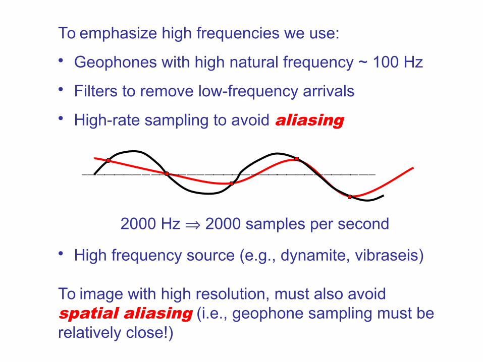
To emphasize high frequencies we use:
• Geophones with high natural frequency ~ 100 Hz
• Filters to remove low-frequency arrivals
• High-rate sampling to avoid aliasing
• High frequency source (e.g., dynamite, vibraseis)
To image with high resolution, must also avoid spatial aliasing (i.e., geophone sampling must be relatively close!)
2000 Hz 2000 samples per second

Reflection Seismic Data Processing:
Step I: Static Correction for elevation, variable weathering &/or water table:
Generally would like to remove effectsof elevation & shallow layer thicknessto emphasize deeper reflections
Vw
V1
V2

Vw
V1
V2
First subtract a correction for low-velocity layer thickness:
Assumes vertical rays, known thickness (from refraction!) & “corrects” travel time to what it would be if the top layer had velocity V1.
(Unsaturated soil Vw ~ 400 m/s;saturated soil V1 ~ 1500 m/s)
hwg
hws
tcorr tobs hws
hwg
Vw
hws
hwg
V1

Vw
V1
V2
Then subtract a correction for elevation differences:
Typically choose elevation datum to be lowest point on the survey. Static correction is a time shift applied to the entire geophone trace! Equivalently can use “refraction static”: Shift head wave arrivals from layer 1 (on each trace) to give slope = 1/V1.es
eg
elevation datum ed
hwg
hws
tcorr tobs hws
hwg
Vw
hws
hwg
V1
es eg 2ed
V1

Static correction: Entire trace is shifted by a constant timeDynamic correction: Different portions of the trace are shifted by different amounts of time
Reflection Seismic Data Processing Step II:
Correction for Normal Move-out (NMO):If we want an image of the subsurface in two-way travel-time(or depth), called a seismic section, we correct for NMO tomove all reflections to where they would be at zero offset.
Could use Dix Eqns:
but for lots of reflections, lots of shots this would involve lotsof travel-time picks and lots of person-time…
Instead we look for approaches that are easier to automate.
TNMO x 2 4h2
Vrms
2h
Vrms

Approach A to Velocity Analysis:
Recall the second-order binomial series approximation to TNMO:
We know x but not t0, Vs. One approach is to use trial-&-error:At every t0, try lots of different “stacking velocities” Vs to find which best “flattens” the reflection arrival:
Vs = 1400
Vs = 1000
Vs = 1800
Vs =
(Simple, but not fully automatic, and will not help to bring out weak reflections).
Table 4-11
5060708090
0 5 10 15 20 25 30
Distance (m)
Tim
e (
ms)
Reflect ion t imes (ms)
Corrected t ime 1 (ms)
Corrected t ime 2 (ms)
Corrected t ime 3 (ms)
TNMO ˙ x2
2t0Vs2
x4
8t03Vs
4

Approach B to Velocity Analysis:
Similar to Approach A, in that we try lots of t0’s and stackingvelocities Vs… Difference is that for each trial we sum allof the trace amplitudes and find which correction produces thelargest stacked amplitude at time t0.
Peak stack amplitudedefines correct
stacking velocity
Stack amplitude

Approach C to Velocity Analysis:
• Assume every t0 is the onset of a reflection.
• Window every geophone trace at plus/minus a few ms and compare (“cross-correlate”) all traces within the window
The stacking velocity Vs that yields the most similar waveformin all windows gives highest cross-corr & is used for that t0.
S1 S2 S3 S4 S6S5
S7S8 S9
TNMO ˙ x2
2t0Vs2
x4
8t03Vs
4

Step III: Stacking Common Depth Point Gathers:
For industry seismic, usually have lots of shots & lots ofreceivers at every shot. Reflection signal is amplified andnoise is attenuated by stacking, i.e., summing traces fromdifferent source-receiver pairs in an optimal way. Most commonly use Common Depth Point (CDP) stacks:First correct forNMO (aftervelocity analysisto determine beststack velocity Vs
for each t0), thensum all traces that have the same mid-point and place the summed tracesat that point on theimage.

After NMO correction and CDP stack, have a seismic section: horizontal layers all image correctly in two-way travel-time. If layers truly are ~ horizontal, processing can end here.
But what if layers dip?
h1
V1
Thereflecting point isno longer directly below the source,and NMO correction maps “true” to an apparent reflecting point vertically beneath the source. For stacksfrom a multiple source-receiver array, this maps dipping reflectors to horizons that are shallower and may have shallower dip than the true horizons.
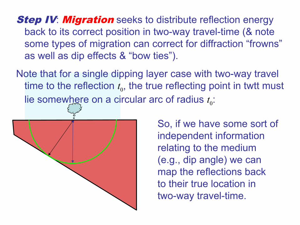
Step IV: Migration seeks to distribute reflection energy back to its correct position in two-way travel-time (& note some types of migration can correct for diffraction “frowns” as well as dip effects & “bow ties”).
Note that for a single dipping layer case with two-way travel time to the reflection t0, the true reflecting point in twtt must lie somewhere on a circular arc of radius t0:
So, if we have some sort ofindependent information relating to the medium(e.g., dip angle) we canmap the reflections back to their true location intwo-way travel-time.
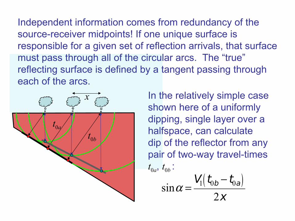
Independent information comes from redundancy of thesource-receiver midpoints! If one unique surface isresponsible for a given set of reflection arrivals, that surfacemust pass through all of the circular arcs. The “true”reflecting surface is defined by a tangent passing througheach of the arcs.
In the relatively simple caseshown here of a uniformlydipping, single layer over a halfspace, can calculatedip of the reflector from any pair of two-way travel-times t0a, t0b :
t0b
t0a
x
sin V1 t0b t0a
2x

Other processing steps may include:
• Amplitude adjustments: Small changes in impedance contrast can change amplitudes significantly, make reflections visually hard to follow: Some software will normalize a reflection on one trace to that on the next.
• Frequency adjustments: Filter to remove unwanted low-frequency info (e.g. ground roll) digitally after the fact instead of a priori (so information is preserved if needed!)
• Transmission adjustments: “Inverse filtering” to upweight desired higher frequency (higher resolution) info that is attenuated more by the Earth medium; also filtering to remove effects of multiples
• Conversion of time section to depth section, and depth migration

Time Migrated seismic image
Depth Migrated seismic image