In Defense of the Triplet Loss for Person Re-Identification

Alexander Hermans∗, Lucas Beyer∗ and Bastian LeibeVisual Computing InstituteRWTH Aachen University

last@vision.rwth-aachen.org

Abstract

In the past few years, the field of computer vision hasgone through a revolution fueled mainly by the adventof large datasets and the adoption of deep convolutionalneural networks for end-to-end learning. The person re-identification subfield is no exception to this. Unfortunately,a prevailing belief in the community seems to be that thetriplet loss is inferior to using surrogate losses (classifi-cation, verification) followed by a separate metric learn-ing step. We show that, for models trained from scratch aswell as pretrained ones, using a variant of the triplet loss toperform end-to-end deep metric learning outperforms mostother published methods by a large margin.

1. Introduction

In recent years, person re-identification (ReID) has at-tracted significant attention in the computer vision commu-nity. Especially with the rise of deep learning, many newapproaches have been proposed to achieve this task [40, 8,42, 31, 39, 10, 52, 4, 46, 20, 54, 35]1. In many aspectsperson ReID is similar to image retrieval, where significantprogress has been made and where deep learning has re-cently introduced a lot of changes. One prominent examplein the recent literature is FaceNet [29], a convolutional neu-ral network (CNN) used to learn an embedding for faces.The key component of FaceNet is to use the triplet loss, asintroduced by Weinberger and Saul [41], for training theCNN as an embedding function. The triplet loss optimizesthe embedding space such that data points with the sameidentity are closer to each other than those with differentidentities. A visualization of such an embedding is shownin Figure 1.

Several approaches for person ReID have already usedsome variant of the triplet loss to train their models [17,9, 28, 8, 40, 31, 33, 26, 6, 25], with moderate success. The

∗Equal contribution. Ordering determined by a last minute coin flip.1A nice overview of the field is given by a recent survey paper [51].

Figure 1: A small crop of the Barnes-Hut t-SNE [38] ofour learned embeddings for the Market-1501 test-set. Thetriplet loss learns semantically meaningful features.

recently most successful person ReID approaches argue thata classification loss, possibly combined with a verificationloss, is superior for the task [6, 51, 10, 52, 22]. Typically,these approaches train a deep CNN using one or multipleof these surrogate losses and subsequently use a part of thenetwork as a feature extractor, combining it with a metriclearning approach to generate final embeddings. Both ofthese losses have their problems, though. The classificationloss necessitates a growing number of learnable parametersas the number of identities increases, most of which willbe discarded after training. On the other hand, many of thenetworks trained with a verification loss have to be usedin a cross-image representation mode, only answering thequestion “How similar are these two images?”. This makes

1

arX

iv:1

703.

0773

7v4

[cs

.CV

] 2

1 N

ov 2

017

using them for any other task, such as clustering or retrieval,prohibitively expensive, as each probe has to go through thenetwork paired up with every gallery image.

In this paper we show that, contrary to current opin-ion, a plain CNN with a triplet loss can outperform currentstate-of-the-art approaches on the CUHK03 [21], Market-1501 [50] and MARS [49] datasets. The triplet loss allowsus to perform end-to-end learning between the input imageand the desired embedding space. This means we directlyoptimize the network for the final task, which renders an ad-ditional metric learning step obsolete. Instead, we can sim-ply compare persons by computing the Euclidean distanceof their embeddings.

A possible reason for the unpopularity of the triplet lossis that, when applied naıvely, it will indeed often producedisappointing results. An essential part of learning usingthe triplet loss is the mining of hard triplets, as otherwisetraining will quickly stagnate. However, mining such hardtriplets is time consuming and it is unclear what defines“good” hard triplets [29, 31]. Even worse, selecting toohard triplets too often makes the training unstable. We showhow this problem can be alleviated, resulting in both fastertraining and better performance. We systematically analyzethe design space of triplet losses, and evaluate which oneworks best for person ReID. While doing so, we place twopreviously proposed variants [9, 32] into this design spaceand discuss them in more detail in Section 2. Specifically,we find that the best performing version has not been usedbefore. Furthermore we also show that a margin-less formu-lation performs slightly better, while removing one hyper-parameter.

Another clear trend seems to be the use of pretrainedmodels such as GoogleNet [36] or ResNet-50 [14]. In-deed, pretrained models often obtain great scores for personReID [10, 52], while ever fewer top-performing approachesuse networks trained from scratch [21, 1, 8, 42, 31, 39, 4].Some authors even argue that training from scratch isbad [10]. However, using pretrained networks also leads toa design lock-in, and does not allow for the exploration ofnew deep learning advances or different architectures. Weshow that, when following best practices in deep learning,networks trained from scratch can perform competitivelyfor person ReID. Furthermore, we do not rely on networkcomponents specifically tailored towards person ReID, buttrain a plain feed-forward CNN, unlike many other ap-proaches that train from scratch [21, 1, 39, 42, 34, 20, 48].Indeed, our networks using pretrained weights obtain thebest results, but our far smaller architecture obtains re-spectable scores, providing a viable alternative for ap-plications where person ReID needs to be performed onresource-constrained hardware, such as embedded devices.

In summary our contribution is twofold: Firstly we intro-duce variants of the classic triplet loss which render mining

of hard triplets unnecessary and we systematically evalu-ate these variants. And secondly, we show how, contraryto the prevailing opinion, using a triplet loss and no speciallayers, we achieve state-of-the-art results both with a pre-trained CNN and with a model trained from scratch. Thishighlights that a well designed triplet loss has a significantimpact on the result, on par with other architectural novel-ties, hopefully enabling other researchers to gain the full po-tential of the previously often dismissed triplet loss. This isan important result, highlighting that a well designed tripletloss has a significant impact on model performance—on parwith other architectural novelties—hopefully enabling otherresearchers to gain the full potential of the previously oftendismissed triplet loss.

2. Learning Metric Embeddings, the TripletLoss, and the Importance of Mining

The goal of metric embedding learning is to learn a func-tion fθ(x) : RF → RD which maps semantically similarpoints from the data manifold in RF onto metrically closepoints in RD. Analogously, fθ should map semanticallydifferent points in RF onto metrically distant points in RD.The function fθ is parametrized by θ and can be anythingranging from a linear transform [41, 23, 45, 28] to com-plex non-linear mappings usually represented by deep neu-ral networks [9, 8, 10]. Let D(x, y) : RD × RD → Rbe a metric function measuring distances in the embeddingspace. For clarity we use the shortcut notation Di,j =D(fθ(xi), fθ(xj)), where we omit the indirect dependenceof Di,j on the parameters θ. As is common practice, allloss-terms are divided by the number of summands in abatch; we omit this term in the following equations for con-ciseness.

Weinberger and Saul [41] explore this topic with the ex-plicit goal of performing k-nearest neighbor classification inthe learned embedding space and propose the “Large Mar-gin Nearest Neighbor loss” for optimizing fθ:

LLMNN(θ) = (1− µ)Lpull(θ) + µLpush(θ), (1)

which is comprised of a pull-term, pulling data points i to-wards their target neighbor T (i) from the same class, anda push-term, pushing data points from a different class kfurther away:

Lpull(θ) =∑

i,j∈T (i)

Di,j , (2)

Lpush(θ) =∑a,n

ya 6=yn

[m+Da,T (a) −Da,n

]+. (3)

Because the motivation was nearest-neighbor classification,allowing disparate clusters of the same class was an explicit

goal, achieved by choosing fixed target neighbors at the on-set of training. Since this property is harmful for retrievaltasks such as face and person ReID, FaceNet [29] proposeda modification of LLMNN(θ) called the “Triplet loss”:

Ltri(θ) =∑a,p,n

ya=yp 6=yn

[m+Da,p −Da,n]+ . (4)

This loss makes sure that, given an anchor point xa, theprojection of a positive point xp belonging to the same class(person) ya is closer to the anchor’s projection than that ofa negative point belonging to another class yn, by at least amargin m. If this loss is optimized over the whole datasetfor long enough, eventually all possible pairs (xa, xp) willbe seen and be pulled together, making the pull-term re-dundant. The advantage of this formulation is that, whileeventually all points of the same class will form a singlecluster, they are not required to collapse to a single point;they merely need to be closer to each other than to any pointfrom a different class.

A major caveat of the triplet loss, though, is that as thedataset gets larger, the possible number of triplets growscubically, rendering a long enough training impractical. Tomake matters worse, fθ relatively quickly learns to correctlymap most trivial triplets, rendering a large fraction of alltriplets uninformative. Thus mining hard triplets becomescrucial for learning. Intuitively, being told over and overagain that people with differently colored clothes are dif-ferent persons does not teach one anything, whereas seeingsimilarly-looking but different people (hard negatives), orpictures of the same person in wildly different poses (hardpositives) dramatically helps understanding the concept of“same person”. On the other hand, being shown only thehardest triplets would select outliers in the data unpropor-tionally often and make fθ unable to learn “normal” asso-ciations, as will be shown in Table 1. Examples of typi-cal hard positives, hard negatives, and outliers are shownin the Supplementary Material. Hence it is common toonly mine moderate negatives [29] and/or moderate pos-itives [31]. Regardless of which type of mining is beingdone, it is a separate step from training and adds consider-able overhead, as it requires embedding a large fraction ofthe data with the most recent fθ and computing all pairwisedistances between those data points.

In a classical implementation, once a certain set of Btriplets has been chosen, their images are stacked into abatch of size 3B, for which the 3B embeddings are com-puted, which are in turn used to create B terms contributingto the loss. Given the fact that there are up to 6B2 − 4Bpossible combinations of these 3B images that are validtriplets, using only B of them seems wasteful. With thisrealization, we propose an organizational modification tothe classic way of using the triplet loss: the core idea is to

form batches by randomly sampling P classes (person iden-tities), and then randomly sampling K images of each class(person), thus resulting in a batch of PK images.2 Now, foreach sample a in the batch, we can select the hardest posi-tive and the hardest negative samples within the batch whenforming the triplets for computing the loss, which we callBatch Hard:

LBH(θ;X) =

all anchors︷ ︸︸ ︷P∑i=1

K∑a=1

[m+

hardest positive︷ ︸︸ ︷maxp=1...K

D(fθ(x

ia), fθ(x

ip))

(5)

− minj=1...Pn=1...Kj 6=i

D(fθ(x

ia), fθ(x

jn))

︸ ︷︷ ︸hardest negative

]+,

which is defined for a mini-batch X and where a data pointxij corresponds to the j-th image of the i-th person in thebatch.

This results in PK terms contributing to the loss, athreefold3 increase over the traditional formulation. Addi-tionally, the selected triplets can be considered moderatetriplets, since they are the hardest within a small subset ofthe data, which is exactly what is best for learning with thetriplet loss.

This new formulation of sampling a batch immediatelysuggests another alternative, that is to simply use all possi-ble PK(PK −K)(K − 1) combinations of triplets, whichcorresponds to the strategy chosen in [9] and which we callBatch All:

LBA(θ;X) =

all anchors︷ ︸︸ ︷P∑i=1

K∑a=1

all pos.︷︸︸︷K∑p=1p 6=a

all negatives︷ ︸︸ ︷P∑j=1j 6=i

K∑n=1

[m+ di,a,pj,a,n

]+, (6)

di,a,pj,a,n = D(fθ(x

ia), fθ(x

ip))−D

(fθ(x

ia), fθ(x

jn)).

At this point, it is important to note that both LBH andLBA still exactly correspond to the standard triplet lossin the limit of infinite training. Both the max and minfunctions are continuous and differentiable almost every-where, meaning they can be used in a model trained bystochastic (sub-)gradient descent without concern. In fact,they are already widely available in popular deep-learningframeworks for the implementation of max-pooling and theReLU [11] non-linearity.

Most similar to our batch hard and batch all losses isthe Lifted Embedding loss [32], which fills the batch with

2In all experiments we choose B, P , and K in such a way that 3B isclose to PK, e.g. 3 · 42 ≈ 32 · 4.

3Because PK ≈ 3B, see footnote 2

triplets but considers all but the anchor-positive pair as neg-atives:

LL(θ;X) =∑

(a,p)∈X

[Da,p+log

∑n∈X

n 6=a,n6=p

(em−Da,n + em−Dp,n

) ]+.

While [32] motivates a “hard”-margin loss similar to LBHand LBA, they end up optimizing the smooth bound of itgiven in the above equation. Additionally, traditional 3Bbatches are considered, thus using all possible negatives,but only one positive pair per triplet. This leads us to pro-pose a generalization of the Lifted Embedding loss basedon PK batches which considers all anchor-positive pairs asfollows:

LLG(θ;X) =

all anchors︷ ︸︸ ︷P∑i=1

K∑a=1

[log

all positives︷ ︸︸ ︷K∑p=1p 6=a

eD(fθ(xia),fθ(x

ip)) (7)

+ log

P∑j=1j 6=i

K∑n=1

em−D(fθ(xia),fθ(x

jn))

︸ ︷︷ ︸all negatives

]+.

Distance Measure. Throughout this section, we havereferred to D(a, b) as the distance function between aand b in the embedding space. In most related works,the squared Euclidean distance D (fθ(xi), fθ(xj)) =

‖fθ(xi)− fθ(xj)‖22 is used as metric, although nothingin the above loss definitions precludes using any other(sub-)differentiable distance measure. While we do nothave a side-by-side comparison, we noticed during initialexperiments that using the squared Euclidean distance madethe optimization more prone to collapsing, whereas usingthe actual (non-squared) Euclidean distance was more sta-ble. We hence used the Euclidean distance throughout allour experiments presented in this paper. In addition, squar-ing the Euclidean distance makes the margin parameter lessinterpretable, as it does not represent an absolute distanceanymore.

Note that when forcing the embedding’s norm to one,using the squared Euclidean distance corresponds to usingthe cosine-similarity, up to a constant factor of two. We didnot use a normalizing layer in any of our final experiments.For one, it does not dramatically regularize the network byreducing the available embedding space: the space spannedby all D-dimensional vector of fixed norm is still a D − 1-dimensional volume. Worse, an output-normalization layercan actually hide problems in the training, such as slowlycollapsing or exploding embeddings.

Soft-margin. The role of the hinge function [m+ •]+is to avoid correcting “already correct” triplets. But in

person ReID, it can be beneficial to pull together samplesfrom the same class as much as possible [45, 8], espe-cially when working on tracklets such as in MARS [49].For this purpose, it is possible to replace the hinge func-tion by a smooth approximation using the softplus function:ln(1 + exp(•)), for which numerically stable implementa-tions are commonly available as log1p. The softplus func-tion has similar behavior to the hinge, but it decays expo-nentially instead of having a hard cut-off, we hence refer toit as the soft-margin formulation.

Summary. In summary, the novel contributions proposedin this paper are the batch hard loss and its soft margin ver-sion. In the following section we evaluate them experimen-tally and show that, for ReID, they achieve superior perfor-mance compared to both the traditional triplet loss and thepreviously published variants of it [9, 32].

3. Experiments

Our experimental evaluation is split up into three mainparts. The first section evaluates different variations of thetriplet loss, including some hyper-parameters, and identi-fies the setting that works best for person ReID. This eval-uation is performed on a train/validation split we createbased on the MARS training set. The second section showsthe performance we can attain based on the selected vari-ant of the triplet loss. We show state-of-the-art results onthe CUHK03, Market-1501 and MARS test sets, based ona pretrained network and a network trained from scratch.Finally, the third section discusses advantages of trainingmodels from scratch with respect to real-world use cases.

3.1. Datasets

We focus on the Market-1501 [50] and MARS [49]datasets, the two largest person ReID datasets currentlyavailable. The Market-1501 dataset contains boundingboxes from a person detector which have been selectedbased on their intersection-over-union overlap with manu-ally annotated bounding boxes. It contains 32 668 imagesof 1501 persons, split into train/test sets of 12 936/19 732images as defined by [50]. The dataset uses both single-and multi-query evaluation, we report numbers for both.

The MARS dataset originates from the same raw data asthe Market-1501 dataset; however, a significant differenceis that the MARS dataset does not have any manually an-notated bounding boxes, reducing the annotation overhead.MARS consist of “tracklets” which have been grouped intoperson IDs manually. It contains 1 191 003 images splitinto train/test sets of 509 914/681 089 images, as definedby [49]. Here, person ReID is no longer performed on aframe-to-frame level, but instead on a tracklet-to-trackletlevel, where feature embeddings are pooled across a track-let, thus it is inherently a multi-query setup.

We use the standard evaluation metrics for both datasets,namely the mean average precision score (mAP) and thecumulative matching curve (CMC) at rank-1 and rank-5. Tocompute these scores we use the evaluation code providedby [55].

Additionally, we show results on the CUHK03 [21]dataset for our pretrained network, using the single shotsetup and average over the provided 20 train/test splits.

3.2. Training

Unless specifically noted otherwise, we use the sametraining procedure across all experiments and on alldatasets. We performed all our experiments using theTheano [5] framework, code is available at redacted.

We use the Adam optimizer [18] with the default hyper-parameter values (ε = 10−3, β1 = 0.9, β2 = 0.999) formost experiments. During initial experiments on our ownMARS validation split (see Sec. 3.4), we ran multiple ex-periments for a very long time and monitored the loss andmAP curves. With this information, we decided to fix thefollowing exponentially decaying training schedule, whichdoes not disadvantage any setup, for all experiments pre-sented in this paper:

ε(t) =

{ε0 if t ≤ t0ε00.001

t−t0t1−t0 if t0 ≤ t ≤ t1

(8)

with ε0 = 10−3, t0 = 15 000, and t1 = 25 000, stoppingtraining when reaching t1. We also set β1 = 0.5 whenentering the decay schedule at t0, as is common practice [2].

In the Supplementary Material, we provide a detaileddiscussion of various interesting effects we regularly ob-served during training, providing hands-on guidance forother researchers.

3.3. Network Architectures

For our main results we use two different architectures,one based on a pretrained network and one which we trainfrom scratch.

Pretrained. We use the ResNet-50 architecture and theweights provided by He et al. [14]. We discard the last layerand add two fully connected layers for our task. The firsthas 1024 units, followed by batch normalization [16] andReLU [11], the second goes down to 128 units, our finalembedding dimension. Trained with our batch hard tripletloss, we call this model TriNet. Due to the size of this net-work (25.74M parameters), we had to limit our batch sizeto 72, containing P = 18 persons with K = 4 images each.For these pretrained experiments, ε0 = 10−3 proved to betoo high, causing the models to diverge within few itera-tions. We thus reduced ε0 to 3 · 10−4 which worked fine onall datasets.

Trained from Scratch. To show that training from scratchdoes not necessarily result in poor performance, we also de-signed a network called LuNet which we train from scratch.LuNet follows the style of ResNet-v2, but uses leaky ReLUnonlinearities, multiple 3 × 3 max-poolings with stride 2instead of strided convolutions, and omits the final average-pooling of feature-maps in favor of a channel-reducing fi-nal res-block. An in-depth description of the architectureis given in the Supplementary Material. As the network ismuch more lightweight (5.00M parameters) than its pre-trained sibling, we sample batches of size 128, containingP = 32 persons with K = 4 images each.

3.4. Triplet Loss

Our initial experiments test the different variants oftriplet training that we discussed in Sec. 2. In order not toperform model-selection on the test set, we randomly sam-ple a validation set of 150 persons from the MARS trainingset, leaving the remaining 475 persons for training. In orderto make this exploration tractable, we run all of these exper-iments using the smaller LuNet trained from scratch on im-ages downscaled by a factor of two. Since our goal here isto explore triplet loss formulations, as opposed to reachingtop performance, we do not perform any data augmentationin these experiments.

Table 1 shows the resulting mAP and rank-1 scores forthe different formulations at multiple margin values, andwith a soft-margin where applicable. Consistent with re-sults reported in several recent papers [10, 9, 6], the vanillatriplet loss with randomly sampled triplets performs poorly.When performing simple offline hard-mining (OHM), thescores sometimes increase dramatically, but the trainingalso fails to learn useful embeddings for multiple marginvalues. This problem is well-known [29, 31] and has beendiscussed in Sec. 2. While the idea of learning embed-dings using triplets is theoretically pleasing, this practi-cal finnickyness, coupled with the considerable increase intraining time due to non-parallelizable offline mining (from7 h to 20 h in our experiments), makes learning with vanillatriplets rather unattractive.

Considering the long training times, it is nice to see thatall proposed triplet re-formulations perform similarly to orbetter than the best OHM run. The key observation is thatthe (semi) hard-mining happens within the batch and thuscomes at almost no additional runtime cost.

Perhaps surprisingly, the batch hard variant (Eq. 5) con-sistently outperforms the batch all variant (Eq. 6) previouslyused by several authors [9, 40]. We suspect this is due to thefact that in the latter, many of the possible triplets in a batchare zero, essentially “washing out” the few useful contribut-ing terms during averaging. To test this hypothesis, we alsoran experiments where we only average the non-zero lossterms (marked by 6= 0 in Table 1); this performs much better

margin 0.1 margin 0.2 margin 0.5 margin 1.0 soft margin

mAP rank-1 mAP rank-1 mAP rank-1 mAP rank-1 mAP rank-1

Triplet (Ltri) 40.80 59.23 41.71 60.78 43.51 60.87 43.61 61.63 48.40 66.37Triplet (Ltri) + OHM 16.6* 36.6* 61.40 82.95 32.0* 57.1* 41.45 59.42 46.63 65.43Batch hard (LBH) 65.09 83.51 65.27 84.55 65.12 83.39 63.78 82.48 65.77 84.69Batch hard (LBH6=0) 63.10 83.04 64.19 83.42 63.71 82.29 64.06 84.50 - -Batch all (LBA) 59.43 79.24 60.48 79.99 60.30 79.52 62.08 80.55 61.04 80.65Batch all (LBA 6=0) 63.29 83.65 64.31 83.37 64.41 83.98 64.06 82.90 - -Lifted 3-pos. (LLG) 64.00 82.71 63.87 82.86 63.61 84.55 64.02 84.17 - -Lifted 1-pos. (LL) [32] 61.95 81.35 63.68 81.73 63.01 82.48 62.28 82.34 - -

Table 1: LuNet scores on our MARS validation split. The best performing loss at a given margin is bold, the best margin for agiven loss is italic, and the overall best combination is highlighted in green. A * denotes runs trapped in a bad local optimum.

in the batch all case. Another interpretation of this modifi-cation is that it dynamically increases the weight of tripletswhich remain active as they get fewer.

The lifted triplet loss LL as introduced by [32] performscompetitively, but is slightly worse than most other formu-lations. As can be seen in the table, our generalization tomultiple positives (Eq. 7), which makes it more similar tothe batch all variant of the triplet, improves upon it overall.

The best score was obtained by the soft-margin variationof the batch hard loss. We use this loss in all our furthertriplet experiments. To clarify, here we merely seek the besttriplet loss variation for person ReID, but do not claim thatthis variant works best across all fields. For other tasks suchas image retrieval or clustering, additional experiments willhave to be performed.

3.5. Performance Evaluation

Here, we present the main experiments of this paper.We perform all following experiments using the batch hardvariant LBH of the triplet loss and the soft margin, since thissetup performed best during the exploratory phase.

Batch Generation and Augmentation. Since our batchhard triplet loss requires slightly different mini-batches, wesample random PK-style batches by first randomly sam-pling P person identities uniformly without replacement.For each person, we then sample K images, without re-placement whenever possible, otherwise replicating imagesas necessary.

We follow common practice by using random crops andrandom horizontal flips during training [19, 1]. Specifi-cally, we resize all images of size H ×W to 1 1

8 (H ×W ),of which we take random crops of size H × W , keepingtheir aspect ratio intact. For all pretrained networks weset H = 256,W = 128 on Market-1501 and MARS andH = 256,W = 96 on CUHK03, whereas for the networkstrained from scratch we set H = 128,W = 64.

We apply test-time augmentation in all our experiments.Following [19], we deterministically average over the em-

beddings from five crops and their flips. This typically givesan improvement of 3% in the mAP score; a more detailedanalysis can be found in the Supplementary Material.

Combination of Embeddings. For test-time augmenta-tion, multi-query evaluation, and tracklet-based evaluation,the embeddings of multiple images need to be combined.

While the learned clusters have no reason to be Gaussian,their convex hull is trained to only contain positive points.Thus, a convex combination of multiple embeddings cannotget closer to a negative embedding than any of the originalones, which is not the case for a non-convex combinationsuch as max-pooling. For this reason, we suggest combin-ing triplet-based embeddings by using their mean. For ex-ample, combining tracklet-embeddings using max-poolingled to an 11.4% point decrease in mAP on MARS.

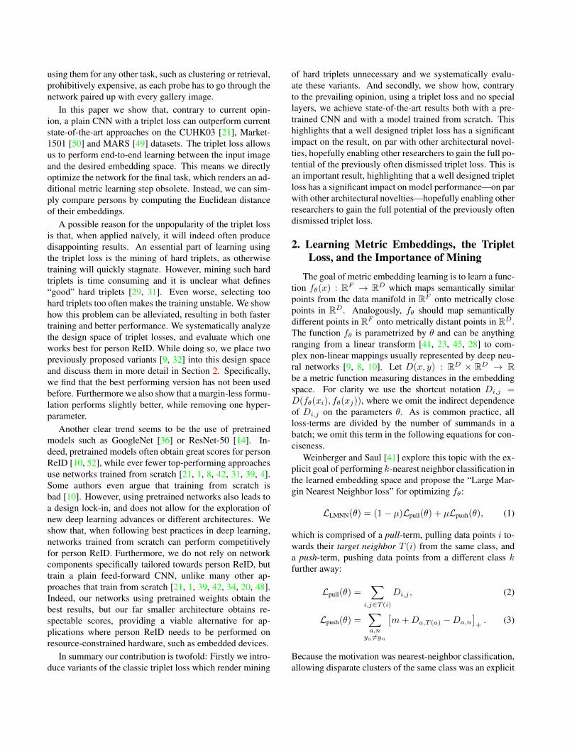
Comparison to State-of-the-Art. Tables 2 and 3 compareour results to a set of related, top performing approaches onMarket-1501 and MARS, and CUHK03, respectively. Wedo not include approaches which are orthogonal to ours andcould be integrated in a straightforward manner, such asvarious re-ranking schemes, data augmentation, and regu-larization [3, 43, 54, 7, 47, 53, 56]. These are included inmore exhaustive tables in the Supplementary Material. Thedifferent approaches are categorized into three major types:Identification models (I) that are trained to classify personIDs, Verification models (V) that learn whether an imagepair represents the same person, and methods such as oursthat directly learn an Embedding (E).

We present results for both our pretrained network(TriNet) and the network we trained from scratch (LuNet).As can clearly be seen, TriNet outperforms all current meth-ods. Especially striking is the jump from 41.5% mAP, ob-tained by another ResNet-50 model trained with triplets(DTL [10]), to our 69.14% mAP score in Table 2. SinceGeng et al. [10] do not discus all details of their trainingprocedure when using the triplet loss, we could only specu-late about the reasons for the large performance gap.

Type Market-1501 SQ Market-1501 MQ MARS

mAP rank-1 rank-5 mAP rank-1 rank-5 mAP rank-1 rank-5

TriNet E 69.14 84.92 94.21 76.42 90.53 96.29 67.70 79.80 91.36LuNet E 60.71 81.38 92.34 69.07 87.11 95.16 60.48 75.56 89.70IDE (R) + ML ours I 58.06 78.50 91.18 67.48 85.45 94.12 57.42 72.42 86.21

LOMO + Null Space [45] E 29.87 55.43 - 46.03 71.56 - - - -Gated siamese CNN [39] V 39.55 65.88 - 48.45 76.04 - - - -CAN [25] E 35.9 60.3 - 47.9 72.1 - - - -JLML [22] I 65.5 85.1 - 74.5 89.7 - - - -ResNet 50 (I+V)† [52] I+V 59.87 79.51 90.91 70.33 85.84 94.54 - - -DTL† [10] E 41.5 63.3 - 49.7 72.4 - - - -DTL† [10] I+V 65.5 83.7 - 73.8 89.6 - - - -APR (R, 751)† [24] I 64.67 84.29 93.20 - - - - - -Latent Parts (Fusion) [20] I 57.53 80.31 - 66.70 86.79 - 56.05 71.77 86.57IDE (R) + ML [55] I 49.05 73.60 - - - - 55.12 70.51 -spatial temporal RNN [57] E - - - - - - 50.7 70.6 90.0CNN + Video† [46] I - - - - - - - 55.5 70.2

TriNet (Re-ranked) E 81.07 86.67 93.38 87.18 91.75 95.78 77.43 81.21 90.76LuNet (Re-ranked) E 75.62 84.59 91.89 82.61 89.31 94.48 73.68 78.48 88.74IDE (R) + ML ours (Re-ra.) I 71.38 81.62 89.88 79.78 86.79 92.96 69.50 74.39 85.86IDE (R) + ML (Re-ra.) [55] I 63.63 77.11 - - - - 68.45 73.94 -

Table 2: Scores on both the Market-1501 and MARS datasets. The top and middle contain our scores and those of thecurrent state-of-the-art respectively. The bottom contains several methods with re-ranking [55]. The different types representthe optimization criteria, where I stands for identification, V for verification and E for embedding. All our scores includetest-time augmentation. The best scores are bold. †: Concurrent work only published on arXiv.

Our LuNet model, which we train from scratch, also per-forms very competitively, matching or outperforming mostother baselines. While it does not quite reach the perfor-mance of our pretrained model, our results clearly show thatwith proper training, the flexibility of training models fromscratch (see Sec. 3.6) should not be discarded.

To show that the actual performance boost is indeedgained by the triplet loss and not by other design choices,we train a ResNet-50 model with a classification loss. Thismodel is very similar to the one used in [55] and we thusrefer to it as “IDE (R) ours”, for which we also apply ametric learning step (XQDA [23]). Unfortunately, espe-cially difficult images caused frequent spikes in the loss,which ended up harming the optimization using Adam. Af-ter unsuccessfully trying lower learning rates and clippingextreme loss values, we resorted to Adadelta [44], anothercompetitive optimization algorithm which did not exhibitthese problems. While we combine embeddings through av-erage pooling for our triplet based models, we found max-pooling and normalization to work better for the classifi-cation baseline, consistent with results reported in [49]. AsTable 2 shows, the performance of the resulting model “IDE(R) ours” is still on-par with similar models in the liter-ature. However, the large gap between the identification-

based model and our TriNet clearly demonstrates the ad-vantages of using a triplet loss.

In line with the general trend in the vision community, alldeep learning methods outperform shallow methods usinghand-crafted features. While Table 2 only shows [45] as anon-deep learning method, to the best of our knowledge allothers perform worse.

We also evaluated how our models fare when combinedwith a recent re-ranking approach by Zhong et al. [55]. Thisapproach can be applied on top of any ranking methodsand uses information from nearest neighbors in the galleryto improve the ranking result. As Table 2 shows, our ap-proaches go well with this method and show similar im-provements to those obtained by Zhong et al. [55].

Finally, we evaluate our models on Market-1501 with theprovided 500k additional distractor images. The full experi-ment is described in the Supplementary Material. Even withthese additional distractors, our triplet-based model outper-forms a classification one by 8.4% mAP.

All of these results show that triplet loss embeddings areindeed a valuable tool for person ReID and we expect themto significantly change the way how research will progressin this field.

Type

Labeled Detected

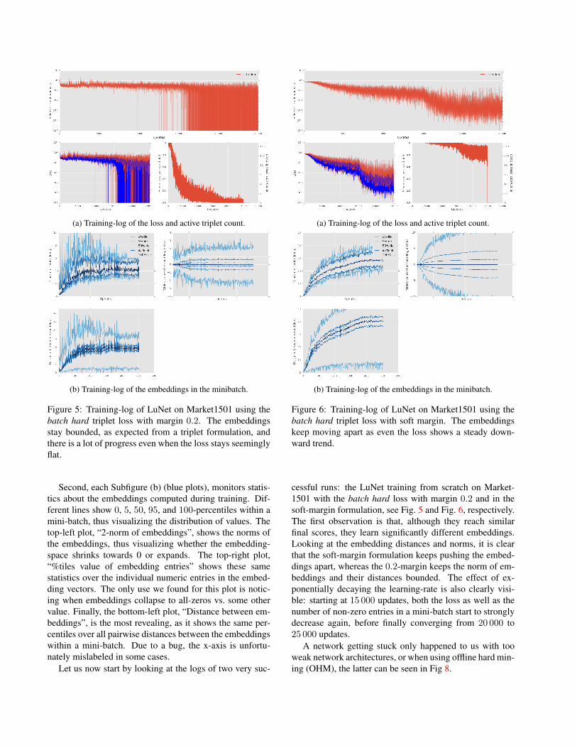
r-1 r-5 r-1 r-5

TriNet E 89.63 99.01 87.58 98.17

Gated siamese CNN [39] V - - 61.8 86.7LOMO + Null Space [45] E 62.55 90.05 54.70 84.75CAN [25] E 77.6 95.2 69.2 88.5Latent Parts (Fusion) [20] I 74.21 94.33 67.99 91.04Spindle Net* [48] I 88.5 97.8 - -JLML [22] I 83.2 98.0 80.6 96.9DTL† [10] I+V 85.4 - 84.1 -ResNet 50 (I+V)† [52] I+V - - 83.4 97.1

Table 3: Scores on CUHK03 for TriNet and a set of recenttop performing methods. The best scores are highlighted inbold. †: Concurrent work only published on arXiv. *: Themethod was trained on several additional datasets.

TriNet LuNet

mAP rank-1 rank-5 mAP rank-1 rank-5

256× 128 69.14 84.92 94.21 - - -128× 64 62.52 79.45 91.06 60.71 81.38 92.3464× 32 47.42 68.08 85.84 57.18 78.21 90.94

Table 4: The effect of input size on mAP and CMC scores.

3.6. To Pretrain or not to Pretrain?

As mentioned before, many methods for person ReIDrely on pretrained networks, following a general trend in thecomputer vision community. Indeed, these models lead toimpressive results, as we also confirmed in this paper withour TriNet model. However, pretrained networks reduce theflexibility to try out new advances in deep learning or tomake task-specific changes in a network. Our LuNet modelclearly suggests that it is also possible to train models fromscratch and obtain competitive scores.

In particular, an interesting direction for ReID could bethe usage of additional input channels such as depth infor-mation, readily available from cheap consumer hardware.However it is unclear how to best integrate such input datainto a pretrained network in a proper way.

Furthermore, the typical pretrained networks are de-signed with accuracy in mind and do not focus on the mem-ory footprint or the runtime of a method. Both are impor-tant factors for real-world robotic scenarios, where typicallypower consumption is a constraint and only less powerfulhardware can be considered [12, 37]. When designing anetwork from scratch, one can directly take this into con-sideration and create networks with a smaller memory foot-print and faster evaluation times.

In principle, our pretrained model can easily be sped upby using half or quarter size input images, since the globalaverage pooling in the ResNet will still produce an outputvector of the same shape. This, however, goes hand in hand

with the question of how to best adapt a pretrained networkto a new task with different image sizes. The typical way ofleveraging pretrained networks is to simply stretch imagesto the fixed expected input size used to train the network,typically 224 × 224 pixels. We used 256 × 128 insteadin order to preserve the aspect ratio of the original image.However, for the Market-1501 dataset, this meant we hadto upscale the images, while if we do not confine ourselvesto pretrained networks we can simply adjust our architec-ture to the dataset size, as we did in the LuNet architecture.However, we hypothesize that a pretrained network has an“intrinsic scale,” for which the learned filters work prop-erly and thus simply using smaller input images will resultin suboptimal performance. To show this, we retrain ourTriNet with 128×64 and 64×32 images. As Table 4 clearlyshows, the performance drops rapidly. At the original imagescale, our LuNet model can almost match the mAP score ofTriNet and already outperforms it when considering CMCscores. At an even smaller image size, LuNet significantlyoutperforms the pretrained model. Since the LuNet perfor-mance only drops by about ∼ 3%, the small images stillhold enough data to perform ReID, but the rather rigid pre-trained weights can no longer adjust to such a data change.This shows that pretrained models are not a solution for ar-bitrary tasks, especially when one wants to train lightweightmodels for small images.

4. DiscussionWe are not the first to use the triplet loss for person ReID.

Ding et al. [9] and Wang et al. [40] use a batch genera-tion and loss formulation which is very similar to our batchall formulation. Wang et al. [40] further combine it with apairwise verification loss. However, in the batch all case, itwas important for us to average only over the active triplets(LBA6=0), which they do not mention. This, in combinationwith their rather small networks, might explain their rela-tively low scores. Cheng et al. [8] propose an “improvedtriplet loss” by introducing another pull term into the loss,penalizing large distances between positive images. Thisformulation is in fact very similar to the original one byWeinberger and Saul [41]. We briefly experimented witha pull term, but the additional weighting hyper-parameterwas not trivial to optimize and it did not improve our re-sults. Several authors suggest learning attributes and ReIDjointly [17, 33, 24, 30], some of which integrate this intotheir embedding dimensions. This is an interesting researchdirection orthogonal to our work. Several other authors alsodefined losses over triplets of images [28, 31, 26], how-ever, they use losses different from the triplet loss we de-fend in this paper, possibly explaining their lower scores.Finally, FaceNet [29] uses a huge batch with moderate min-ing, which can only be done on the CPU, whereas we advo-cate hard mining in a small batch, which has a similar effect

to moderate mining in a large batch, while fitting on a GPUand thus making training significantly more affordable.

5. Conclusion

In this paper we have shown that, contrary to the pre-vailing belief, the triplet loss is an excellent tool for personre-identification. We propose a variant that no longer re-quires offline hard negative mining at almost no additionalcost. Combined with a pretrained network, we set the newstate-of-the-art on three of the major ReID datasets. Fur-thermore, we show that training networks from scratch canlead to very competitive scores. We hope that in future workthe ReID community will build on top of our results andshift more towards end-to-end learning.

Acknowledgments. This work was funded, in parts,by ERC Starting Grant project CV-SUPER (ERC-2012-StG-307432) and the EU project STRANDS (ICT-2011-600623). We would also like to thank the authors of theMarket-1501 and MARS datasets.

References[1] E. Ahmed, M. Jones, and T. K. Marks. An Improved

Deep Learning Architecture for Person Re-Identification. InCVPR, pages 3908–3916, 2015. 2, 6

[2] J. L. Ba, J. R. Kiros, and G. E. Hinton. Layer Normalization.arXiv preprint arXiv:1607.06450, 2016. 5

[3] S. Bai, X. Bai, and Q. Tian. Scalable person re-identificationon supervised smoothed manifold. CVPR, 2017. 6, 15, 16

[4] I. B. Barbosa, M. Cristani, B. Caputo, A. Rognhaugen, andT. Theoharis. Looking Beyond Appearances: SyntheticTraining Data for Deep CNNs in Re-identification. arXivpreprint arXiv:1701.03153, 2017. 1, 2

[5] F. Bastien, P. Lamblin, R. Pascanu, J. Bergstra, I. J. Good-fellow, A. Bergeron, N. Bouchard, and Y. Bengio. Theano:new features and speed improvements. In NIPS W., 2012. 5

[6] W. Chen, X. Chen, J. Zhang, and K. Huang. A Multi-taskDeep Network for Person Re-identification. AAAI, 2017. 1,5

[7] Y. Chen, X. Zhu, and G. Shaogang. Person Re-Identificationby Deep Learning Multi-Scale Representations. In ICCV W.on Cross-domain Human Identification, 2016. 6, 15, 16

[8] D. Cheng, Y. Gong, S. Zhou, J. Wang, and N. Zheng. PersonRe-Identification by Multi-Channel Parts-Based CNN withImproved Triplet Loss Function. In CVPR, 2016. 1, 2, 4, 8

[9] S. Ding, L. Lin, G. Wang, and H. Chao. Deep fea-ture learning with relative distance comparison for personre-identification. Pattern Recognition, 48(10):2993–3003,2015. 1, 2, 3, 4, 5, 8

[10] M. Geng, Y. Wang, T. Xiang, and Y. Tian. Deep Trans-fer Learning for Person Re-identification. arXiv preprintarXiv:1611.05244, 2016. 1, 2, 5, 6, 7, 8, 15, 16

[11] X. Glorot, A. Bordes, and Y. Bengio. Deep Sparse RectifierNeural Networks. In AISTATS, 2011. 3, 5, 16

[12] N. Hawes, C. Burbridge, F. Jovan, L. Kunze, B. Lacerda,L. Mudrova, J. Young, J. Wyatt, D. Hebesberger, T. Kortner,et al. The STRANDS Project: Long-Term Autonomy in Ev-eryday Environments. RAM, 24(3):146–156, 2017. 8

[13] K. He, X. Zhang, S. Ren, and J. Sun. Delving Deep Into Rec-tifiers: Surpassing Human-Level Performance on ImageNetClassification. In ICCV, pages 1026–1034, 2015. 16

[14] K. He, X. Zhang, S. Ren, and J. Sun. Deep Residual Learningfor Image Recognition. In CVPR, 2016. 2, 5, 11

[15] K. He, X. Zhang, S. Ren, and J. Sun. Identity Mappings inDeep Residual Networks. In ECCV, 2016. 16

[16] S. Ioffe and C. Szegedy. Batch normalization: Acceleratingdeep network training by reducing internal covariate shift. InICML, 2015. 5, 16

[17] S. Khamis, C.-H. Kuo, V. K. Singh, V. D. Shet, and L. S.Davis. Joint Learning for Attribute-Consistent Person Re-Identification. In ECCV, 2014. 1, 8

[18] D. P. Kingma and J. Ba. Adam: A Method for StochasticOptimization. In ICLR, 2015. 5

[19] A. Krizhevsky, I. Sutskever, and G. E. Hinton. ImageNetClassification with Deep Convolutional Neural Networks. InNIPS, pages 1097–1105, 2012. 6, 11

[20] D. Li, X. Chen, Z. Zhang, and K. Huang. Learning DeepContext-aware Features over Body and Latent Parts for Per-son Re-identification. In CVPR, 2017. 1, 2, 7, 8, 15, 16

[21] W. Li, R. Zhao, T. Xiao, and X. Wang. DeepReID: DeepFilter Pairing Neural Network for Person Re-Identification.In CVPR, 2014. 2, 5

[22] W. Li, X. Zhu, and S. Gong. Person Re-Identification byDeep Joint Learning of Multi-Loss Classification. In IJCAI,2017. 1, 7, 8, 15, 16

[23] S. Liao, Y. Hu, X. Zhu, and S. Z. Li. Person Re-identificationby Local Maximal Occurrence Representation and MetricLearning. In CVPR, 2015. 2, 7

[24] Y. Lin, L. Zheng, Z. Zheng, Y. Wu, and Y. Yang. Improv-ing person re-identification by attribute and identity learning.arXiv preprint arXiv:1703.07220, 2017. 7, 8, 15

[25] H. Liu, J. Feng, M. Qi, J. Jiang, and S. Yan. End-to-End Comparative Attention Networks for Person Re-identification. Trans. Image Proc., 26(7):3492–3506, 2017.1, 7, 8, 15, 16

[26] J. Liu, Z.-J. Zha, Q. Tian, D. Liu, T. Yao, Q. Ling, and T. Mei.Multi-Scale Triplet CNN for Person Re-Identification. InACMMM, 2016. 1, 8

[27] A. L. Maas, A. Y. Hannun, and A. Y. Ng. Rectifier Nonlin-earities Improve Neural Network Acoustic Models. In ICML,2013. 16

[28] S. Paisitkriangkrai, C. Shen, and A. van den Hengel. Learn-ing to rank in person re-identification with metric ensembles.In CVPR, 2015. 1, 2, 8

[29] F. Schroff, D. Kalenichenko, and J. Philbin. FaceNet: AUnified Embedding for Face Recognition and Clustering. InCVPR, 2015. 1, 2, 3, 5, 8

[30] A. Schumann and R. Stiefelhagen. Person Re-Identificationby Deep Learning Attribute-Complementary Information. InCVPR Workshops, 2017. 8

[31] H. Shi, Y. Yang, X. Zhu, S. Liao, Z. Lei, W. Zheng, and S. Z.Li. Embedding Deep Metric for Person Re-identification: AStudy Against Large Variations. In ECCV, 2016. 1, 2, 3, 5,8

[32] H. O. Song, Y. Xiang, S. Jegelka, and S. Savarese. DeepMetric Learning via Lifted Structured Feature Embedding.In CVPR, 2016. 2, 3, 4, 6

[33] C. Su, S. Zhang, J. Xing, W. Gao, and Q. Tian. Deep At-tributes Driven Multi-camera Person Re-identification. InECCV, 2016. 1, 8

[34] A. Subramaniam, M. Chatterjee, and A. Mittal. DeepNeural Networks with Inexact Matching for Person Re-Identification. In NIPS, pages 2667–2675, 2016. 2

[35] Y. Sun, L. Zheng, W. Deng, and S. Wang. SVDNet for Pedes-trian Retrieval. ICCV, 2017. 1, 15, 16

[36] C. Szegedy, W. Liu, Y. Jia, P. Sermanet, S. Reed,D. Anguelov, D. Erhan, V. Vanhoucke, and A. Rabinovich.Going deeper with convolutions. In CVPR, 2015. 2

[37] R. Triebel, K. Arras, R. Alami, L. Beyer, S. Breuers,R. Chatila, M. Chetouani, D. Cremers, V. Evers, M. Fiore,et al. SPENCER: A Socially Aware Service Robot for Pas-senger Guidance and Help in Busy Airports. In Field andService Robotics, pages 607–622. Springer, 2016. 8

[38] L. Van Der Maaten. Accelerating t-SNE using Tree-BasedAlgorithms. JMLR, 15(1):3221–3245, 2014. 1, 17

[39] R. R. Varior, M. Haloi, and G. Wang. Gated SiameseConvolutional Neural Network Architecture for Human Re-Identification. In ECCV, 2016. 1, 2, 7, 8, 15, 16

[40] F. Wang, W. Zuo, L. Lin, D. Zhang, and L. Zhang. JointLearning of Single-image and Cross-image Representationsfor Person Re-identification. In CVPR, 2016. 1, 5, 8

[41] K. Q. Weinberger and L. K. Saul. Distance Metric Learningfor Large Margin Nearest Neighbor Classification. JMLR,10:207–244, 2009. 1, 2, 8

[42] T. Xiao, H. Li, W. Ouyang, and X. Wang. Learning DeepFeature Representations with Domain Guided Dropout forPerson Re-identification. In CVPR, 2016. 1, 2, 16

[43] R. Yu, Z. Zhou, S. Bai, and X. Bai. Divide and Fuse: ARe-ranking Approach for Person Re-identification. BMVC,2017. 6

[44] M. D. Zeiler. ADADELTA: An Adaptive Learning RateMethod. arXiv preprint arXiv:1212.5701, 2012. 7

[45] L. Zhang, T. Xiang, and S. Gong. Learning a DiscriminativeNull Space for Person Re-identification. In CVPR, 2016. 2,4, 7, 8, 15, 16

[46] W. Zhang, S. Hu, and K. Liu. Learning Compact AppearanceRepresentation for Video-based Person Re-Identification.arXiv preprint arXiv:1702.06294, 2017. 1, 7, 15

[47] Y. Zhang, T. Xiang, T. M. Hospedales, and H. Lu. DeepMutual Learning. arXiv preprint arXiv:1706.00384, 2017.6, 15

[48] H. Zhao, M. Tian, S. Sun, J. Shao, J. Yan, S. Yi, X. Wang,and X. Tang. Spindle Net: Person Re-identification with Hu-man Body Region Guided Feature Decomposition and Fu-sion. In CVPR, 2017. 2, 8, 15, 16

[49] L. Zheng, Z. Bie, Y. Sun, J. Wang, C. Su, S. Wang, andQ. Tian. MARS: A Video Benchmark for Large-Scale Per-son Re-Identification. In ECCV, 2016. 2, 4, 7, 15

[50] L. Zheng, L. Shen, L. Tian, S. Wang, J. Wang, and Q. Tian.Scalable Person Re-Identification: A Benchmark. In ICCV,2015. 2, 4

[51] L. Zheng, Y. Yang, and A. G. Hauptmann. Person Re-identification: Past, Present and Future. arXiv preprintarXiv:1610.02984, 2016. 1

[52] Z. Zheng, L. Zheng, and Y. Yang. A DiscriminativelyLearned CNN Embedding for Person Re-identification.arXiv preprint arXiv:1611.05666, 2016. 1, 2, 7, 8, 11, 12,15, 16

[53] Z. Zheng, L. Zheng, and Y. Yang. Pedestrian AlignmentNetwork for Large-scale Person Re-identification. arXivpreprint arXiv:1707.00408, 2017. 6, 15

[54] Z. Zheng, L. Zheng, and Y. Yang. Unlabeled Samples Gener-ated by GAN Improve the Person Re-identification Baselinein vitro. ICCV, 2017. 1, 6, 15, 16

[55] Z. Zhong, L. Zheng, D. Cao, and S. Li. Re-ranking PersonRe-identification with k-reciprocal Encoding. CVPR, 2017.5, 7, 15

[56] Z. Zhong, L. Zheng, G. Kang, S. Li, and Y. Yang.Random Erasing Data Augmentation. arXiv preprintarXiv:1708.04896, 2017. 6

[57] Z. Zhou, Y. Huang, W. Wang, L. Wang, and T. Tan. See theForest for the Trees: Joint Spatial and Temporal RecurrentNeural Networks for Video-based Person Re-identification.In CVPR, 2017. 7, 15

Supplementary Material

A. Test-time Augmentation

As is good practice in the deep learning community [19,14], we perform test-time augmentation. From each image,we deterministically create five crops of size H ×W : fourcorner crops and one center crop, as well as a horizontallyflipped copy of each. The embeddings of all these ten im-ages are then averaged, resulting in the final embedding fora person. Table 5 shows how five possible settings affect ourscores on the Market-1501 dataset. As expected, the worstoption is to scale the original images to fit the network input(first line), as this shows the network an image type it hasnever seen before. This option is directly followed by notusing any test-time augmentation, i.e. just using the centralcrop. Simply flipping the center crop and averaging the tworesulting embeddings already gives a big boost while onlybeing twice as expensive. The four additional corner cropstypically seem to be less effective, while more expensive,but using both augmentations together gives the best results.For the networks trained with a triplet loss, we gain about3% mAP, while the network trained for identification onlygains about 2% mAP. A possible explanation is that the fea-ture space we learn with the triplet loss could be more suitedto averaging than that of a classification network.

TriNet LuNet IDE (R) Ours

mAP rank-1 mAP rank-1 mAP rank-1

original 65.48 82.51 55.61 76.72 56.29 77.55center 66.29 84.06 57.08 77.94 56.26 77.08center + flip 68.32 84.47 59.31 79.78 57.80 78.715 crops 67.86 84.83 59.00 79.42 56.73 77.295 crops + flip 69.14 84.92 60.71 81.38 58.06 78.50

Table 5: The effect of test-time augmentation on Market-1501.

B. Hard Positives, Hard Negatives and Outliers

Figure 2 shows several outliers in the Market-1501 andMARS datasets. Some issues in MARS are caused bythe tracker-based annotations where bounding boxes some-times span two persons and the tracker partially focuses onthe wrong person. Additionally, some annotation mistakescan be found in both datasets; while some are obvious, someothers are indeed very hard to spot!

In Figure 3 we show some of the most difficult queriesalong with their top-3 retrieved images (containing hardnegatives), as well as their two hardest positives. Whilesome mistakes are easy to spot by a human, others are in-deed not trivial, such as the first row in Figure 3.

PID: 207 PID: 207 PID: 207 PID: 209 PID: 209 PID: 209

PID: 1365 PID: 1365 PID: 1365 PID: 1365 PID: 1365 PID: 1365

PID: 516 PID: 516 PID: 516 PID: 516 PID: 516 PID: 516

Figure 2: Some outliers in the Mars (top two rows) andMarket-1501 (bottom row) datasets. The first row showshigh image overlap between tracklets of two persons. Thesecond row shows a very hard example where a person waswrongly matched across tracklets. The last row shows asimple annotation mistake.

C. Experiments with Distractors

On top of the normal gallery set, the Market-1501 datasetprovides an additional 500k distractors recorded at anothertime. In order to evaluate how such distractors affect per-formance, we randomly sample an increasing number ofdistractors and add them to the original gallery set. Herewe compare to the results from Zheng et al. [52]. Bothour models show a similar behavior to that of their ResNet-50 baseline. Surprisingly, our LuNet model starts out witha slightly better mAP score than the baseline and ends upjust below it, while consistently being better when consid-ering the rank-1 score. This might indeed suggest that theinductive bias from pretraining helps during generalizationto large amounts of unseen data. Nevertheless, all modelsseem to suffer under the increasing gallery set in a similarmanner, albeit none of them fails badly. Especially the factthat in 74.70% of all single-image queries the first imageout of 519 732 gallery images is correctly retrieved is animpressive result.

For reproducibility of the 500k distractor plot (Fig. 4),Table 6 lists the values of the plot.

PID: 1 rank-1 rank-2 rank-3 rank-1450 rank-1967

. . . . . .

PID: 5 rank-1 rank-2 rank-3 rank-470 rank-1130

. . . . . .

PID: 38 rank-1 rank-2 rank-3 rank-1510 rank-2893

. . . . . .

PID: 1026 rank-1 rank-2 rank-3 rank-2302 rank-4611

. . . . . .

PID: 1151 rank-1 rank-2 rank-3 rank-1886 rank-4127

. . . . . .

Figure 3: Some of the hardest queries. The leftmost col-umn shows the query image, followed by the top 3 retrievedimages and the two ground truth matches with the high-est distance to the query images, i.e. the hardest positives.Correctly retrieved images have a green border, mistakes(i.e. hard negatives) have a red border.

TriNet LuNet Res50 (I+V) [52]

Gallery size mAP rank-1 mAP rank-1 mAP rank-1

19 732 69.14 84.92 60.71 81.38 59.87 79.51119 732 61.93 79.69 52.73 75.65 52.28 73.78219 732 58.74 77.88 49.44 73.40 49.11 71.50319 732 56.58 76.34 47.17 71.85 NaN NaN419 732 54.97 75.50 45.57 70.52 NaN NaN519 732 53.63 74.70 44.26 69.74 45.24 68.26

Table 6: Values for the 500k distractor plot.

D. Notes on Network Training

Here we present and discuss several training-logs thatdisplay interesting behavior, as noted in the main paper.

19.73 100 200 300 400 50030

40

50

60

70

80

Gallery Size [K]

mA

P/R

ank-

1[%

]

TriNetLuNet

Res50 (I+V) [52]

Figure 4: 500k distractor set results. Solid lines representthe mAP score, dashed lines the rank-1 score. See Supple-mentary Material for values.

This serves as practical advice of what to monitor for practi-tioners who choose to use a triplet-based loss in their train-ing.

A typical training usually proceeds as follows: initially,all embeddings are pulled together towards their center ofgravity. When they come close to each other, they will“pass” each other to join “their” clusters and, once thiscross-over has happened, training mostly consists of push-ing the clusters further apart and fine-tuning them. The col-lapsing of training happens when the margin is too largeand the initial spread is too small, such that the embeddingsget stuck when trying to pass each other.

Most importantly of all, if any type of hard-triplet min-ing is used, a stagnating loss curve by no means indicatesstagnating progress. As the network learns to solve somehard cases, it will be presented with other hard cases andhence still keep a high loss. We recommend observing thefraction of active triplets in a batch, as well as the norms ofthe embeddings and all pairwise distances.

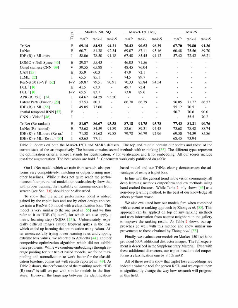
Figures 5, 6, 7, and 8 all show different training logs.Note that while they all share the x-axis since the number ofupdates was kept the same throughout the experiments, they-axes vary for clearer visualization. First, the topmost plotin each Subfigure (a) (“Value of criterion/penalty”) showsall per-triplet values of the optimization criterion (the tripletloss) encountered in each mini-batch. This is shown againin the plot below it on the left (“loss”), with an overlaidlight-blue line representing the batch-mean criterion value,and an overlaid dark-blue line representing the batch’s 5-percentile. To the right of it, the “% non-zero losses inbatch” shows how many entries in the mini-batch had non-zero loss; values are computed up to a precision of 10−5,which explains how it can be below 100% in the soft-margincase. The single final vertical line present in some plotsshould be ignored as a plotting-artifact.

(a) Training-log of the loss and active triplet count.

(b) Training-log of the embeddings in the minibatch.

Figure 5: Training-log of LuNet on Market1501 using thebatch hard triplet loss with margin 0.2. The embeddingsstay bounded, as expected from a triplet formulation, andthere is a lot of progress even when the loss stays seeminglyflat.

Second, each Subfigure (b) (blue plots), monitors statis-tics about the embeddings computed during training. Dif-ferent lines show 0, 5, 50, 95, and 100-percentiles within amini-batch, thus visualizing the distribution of values. Thetop-left plot, “2-norm of embeddings”, shows the norms ofthe embeddings, thus visualizing whether the embedding-space shrinks towards 0 or expands. The top-right plot,“%tiles value of embedding entries” shows these samestatistics over the individual numeric entries in the embed-ding vectors. The only use we found for this plot is notic-ing when embeddings collapse to all-zeros vs. some othervalue. Finally, the bottom-left plot, “Distance between em-beddings”, is the most revealing, as it shows the same per-centiles over all pairwise distances between the embeddingswithin a mini-batch. Due to a bug, the x-axis is unfortu-nately mislabeled in some cases.

Let us now start by looking at the logs of two very suc-

(a) Training-log of the loss and active triplet count.

(b) Training-log of the embeddings in the minibatch.

Figure 6: Training-log of LuNet on Market1501 using thebatch hard triplet loss with soft margin. The embeddingskeep moving apart as even the loss shows a steady down-ward trend.

cessful runs: the LuNet training from scratch on Market-1501 with the batch hard loss with margin 0.2 and in thesoft-margin formulation, see Fig. 5 and Fig. 6, respectively.The first observation is that, although they reach similarfinal scores, they learn significantly different embeddings.Looking at the embedding distances and norms, it is clearthat the soft-margin formulation keeps pushing the embed-dings apart, whereas the 0.2-margin keeps the norm of em-beddings and their distances bounded. The effect of ex-ponentially decaying the learning-rate is also clearly visi-ble: starting at 15 000 updates, both the loss as well as thenumber of non-zero entries in a mini-batch start to stronglydecrease again, before finally converging from 20 000 to25 000 updates.

A network getting stuck only happened to us with tooweak network architectures, or when using offline hard min-ing (OHM), the latter can be seen in Fig 8.

(a) Training-log of the loss and active triplet count.

(b) Training-log of the embeddings in the minibatch.

Figure 7: Training-log of a very small network on Market-1501 using the batch hard triplet loss with soft margin. Thedifficult “packed” phase is clearly visible.

Next, let us turn to Fig. 7, which shows the training-logs of a very small net (not further specified in this paper).We can clearly see that the network first pulls all embed-dings towards their center of gravity, as evidenced by thequickly decreasing embedding norms, entries, as well asdistances in the first few hundred updates. (More visiblewhen zooming-in on a computer.) Once they are all closeto each other, the networks really struggles to make themall “pass each other” to reach “their” clusters. As soon asthis difficult phase is overcome, the embeddings are spreadaround the space to quickly decrease the loss. This is wherethe training becomes “fragile” and prone to collapsing: ifthe embeddings never pass each other, training gets stuck.This behavior can also be observed in Figures 5 and 6, al-though to a much lesser extent, as the network is powerfulenough to quickly overcome this difficult phase.

(a) Training-log of the loss and active triplet count.

(b) Training-log of the embeddings in the minibatch.

Figure 8: Training-log of LuNet on MARS when using of-fline hard mining (OHM) with margin 0.1. This is one of theruns that collapsed and never got past the difficult phase.

E. Extended Comparison TablesWe show extended versions of the two state-of-the-art

comparison tables in the main paper. We add additionalmethods that were left out due to space reasons, or becausethe approaches are orthogonal to ours. The latter could beintegrated with our approach in a straightforward manner.Market-1501 and Mars results are shown in Table 7 andCUHK03 results in Table 8.

Type Market-1501 SQ Market-1501 MQ MARS

mAP rank-1 rank-5 mAP rank-1 rank-5 mAP rank-1 rank-5

TriNet E 69.14 84.92 94.21 76.42 90.53 96.29 67.70 79.80 91.36LuNet E 60.71 81.38 92.34 69.07 87.11 95.16 60.48 75.56 89.70IDE (R) + ML ours I 58.06 78.50 91.18 67.48 85.45 94.12 57.42 72.42 86.21

LOMO + Null Space [45] E 29.87 55.43 - 46.03 71.56 - - - -Gated siamese CNN [39] V 39.55 65.88 - 48.45 76.04 - - - -Spindle Net [48] I - 76.9 91.5 - - - - - -CAN [25] E 35.9 60.3 - 47.9 72.1 - - - -SSM [3] - 68.80 82.21 - 76.18 88.18 - - - -JLML [22] I 65.5 85.1 - 74.5 89.7 - - - -SVDNet [35] I 62.1 82.3 - - - - - - -CNN + DCGAN [54] I 56.23 78.06 - 68.52 85.12 - - - -DPFL [7] I 73.1 88.9 - 80.7 92.3 - - - -ResNet 50 (I+V)† [52] I+V 59.87 79.51 90.91 70.33 85.84 94.54 - - -MobileNet+DML† [47] I 68.83 87.73 - 77.14 91.66 - - - -DTL† [10] E 41.5 63.3 - 49.7 72.4 - - - -DTL† [10] I+V 65.5 83.7 - 73.8 89.6 - - - -APR (R, 751)† [24] I 64.67 84.29 93.20 - - - - - -PAN† [53] I 63.35 82.81 - 71.72 88.18 - - - -IDE (C) + ML [49] I - - - - - - 47.6 65.3 82.0Latent Parts (Fusion) [20] I 57.53 80.31 - 66.70 86.79 - 56.05 71.77 86.57IDE (R) + ML [55] I 49.05 73.60 - - - - 55.12 70.51 -Spatial-Temporal RNN [57] E - - - - - - 50.7 70.6 90.0CNN + Video† [46] I - - - - - - - 55.5 70.2

TriNet (Re-ranked) E 81.07 86.67 93.38 87.18 91.75 95.78 77.43 81.21 90.76LuNet (Re-ranked) E 75.62 84.59 91.89 82.61 89.31 94.48 73.68 78.48 88.74IDE (R) + ML ours (Re-ra.) I 71.38 81.62 89.88 79.78 86.79 92.96 69.50 74.39 85.86IDE (R) + ML (Re-ra.) [55] I 63.63 77.11 - - - - 68.45 73.94 -PAN (Re-ra.)† [53] I 76.65 85.78 - 83.79 89.79 - - - -

Table 7: Scores on both the Market-1501 and MARS datasets. The top and middle contain our scores and those of thecurrent state-of-the-art respectively. The bottom contains several methods with re-ranking [55]. The different types representthe optimization criteria, where I stands for identification, V for verification and E for embedding. All our scores includetest-time augmentation. The best scores are bold. †: Concurrent work only published on arXiv.

Type

Labeled Detected

r-1 r-5 r-1 r-5

TriNet E 89.63 99.01 87.58 98.17

Gated siamese CNN [39] V - - 61.8 86.7DGD* [42] I 75.3 - - -LOMO + Null Space [45] E 62.55 90.05 54.70 84.75SSM [3] - 76.6 94.6 72.7 92.4CAN [25] E 77.6 95.2 69.2 88.5Latent Parts (Fusion) [20] I 74.21 94.33 67.99 91.04Spindle Net* [48] I 88.5 97.8 - -JLML [22] I 83.2 98.0 80.6 96.9SVDNet [35] I - - 81.8 -CNN + DCGAN [54] I - - 84.6 97.6DPFL [7] I 82.8 - 82.0 -DTL† [10] I+V 85.4 - 84.1 -ResNet 50 (I+V)† [52] I+V - - 83.4 97.1

Table 8: Scores on CUHK03 for TriNet and a set of recenttop performing methods. The best scores are highlighted inbold. †: Concurrent work only published on arXiv. *: Themethod was trained on several additional datasets.

F. LuNet’s ArchitectureThe details of the LuNet architecture for training from

scratch can be seen in Table 9. The input image has threechannels and spatial dimensions 128×64. Most Res-blocksare of the “bottleneck” type [15], meaning for given num-bers n1, n2, n3 in the table, they consist of a 1×1 convo-lution from the number of input channels n1 to the numberof intermediate channels n2, followed by a 3×3 convolutionkeeping the number of channel constant, and finally another1×1 convolution going from n2 channels to n3 channels.Only the last Res-block, whose exact filter sizes are givenin the table, is an exception to this. All ReLUs, includingthose in Res-blocks, are leaky [27] by a factor of 0.3; al-though we do not have side-by-side experiments comparingthe benefits, we expect them to be minor. All convolutionalweights are initialized following He et al. [13], whereaswe initialized the final Linear layers following Glorot etal. [11]. Batch-normalization [16] is essential to train sucha network, and makes the exact initialization less important.

Type Size

Conv 128×7×7×3Res-block 128, 32, 128MaxPool pool 3×3, stride (2×2), padding (1×1)

Res-block 128, 32, 128Res-block 128, 32, 128Res-block 128, 64, 256MaxPool pool 3×3, stride (2×2), padding (1×1)

Res-block 256, 64, 256Res-block 256, 64, 256MaxPool pool 3×3, stride (2×2), padding (1×1)Res-block 256, 64, 256Res-block 256, 64, 256Res-block 256, 128, 512MaxPool pool 3×3, stride (2×2), padding (1×1)

Res-block 512, 128, 512Res-block 512, 128, 512MaxPool pool 3×3, stride (2×2), padding (1×1)

Res-block 512×(3×3×512), 128×(3×3×512)Linear 1024×512Batch-Norm 512ReLULinear 512×128

Table 9: The architecture of LuNet.

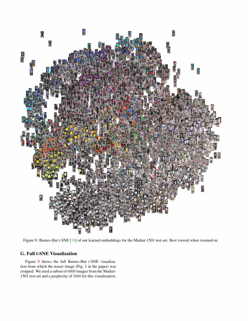
Figure 9: Barnes-Hut t-SNE [38] of our learned embeddings for the Market-1501 test-set. Best viewed when zoomed-in.

G. Full t-SNE VisualizationFigure 9 shows the full Barnes-Hut t-SNE visualiza-

tion from which the teaser image (Fig. 1 in the paper) wascropped. We used a subset of 6000 images from the Market-1501 test-set and a perplexity of 5000 for this visualization.