1

Laser Interferometer Space Antenna (LISA) Mission Concept

Document Number: LISA-PRJ-RP-0001

May 4, 2009

Issue: 0 Revision: 0

2

TABLE OF CONTENTS

1  PURPOSE ..................................................................................................................4 

2  SCIENCE OVERVIEW................................................................................................5 

2.1  Sources .................................................................................................................................................................5 

2.2  Science Objectives ...............................................................................................................................................7 

3  SCIENCE REQUIREMENTS......................................................................................9 

4  MEASUREMENT CONCEPT ...................................................................................14 

4.1  What’s to be measured .....................................................................................................................................14 

4.2  How it’s measured.............................................................................................................................................15 

5  SCIENCE INSTRUMENTATION ..............................................................................17 

5.1  Interferometry ...................................................................................................................................................19 5.1.1  What it does.................................................................................................................................................19 

5.1.1.1  Lasers...................................................................................................................................................19 5.1.1.2  Laser Frequency Noise ........................................................................................................................20 5.1.1.3  Beam Steering and Combination.........................................................................................................20 5.1.1.4  Ranging................................................................................................................................................21 5.1.1.5  Photodetectors .....................................................................................................................................21 5.1.1.6  Phase Measurement .............................................................................................................................21 5.1.1.7  Timing .................................................................................................................................................21 

5.1.2  What it takes to do it ...................................................................................................................................22 5.1.2.1  Laser subsystem...................................................................................................................................22 5.1.2.2  Laser frequency control subsystem .....................................................................................................23 5.1.2.3  Optical bench.......................................................................................................................................24 5.1.2.4  Telescope.............................................................................................................................................26 5.1.2.5  Pointing mechanisms...........................................................................................................................26 5.1.2.6  Photoreceivers .....................................................................................................................................26 5.1.2.7  Phase measurement subsystem............................................................................................................26 

5.2  Disturbance Reduction .....................................................................................................................................27 5.2.1  What it does.................................................................................................................................................27 

5.2.1.1  Gravitational Reference Sensor ...........................................................................................................28 5.2.1.2  Microthrusters......................................................................................................................................29 5.2.1.3  DRS control laws.................................................................................................................................30 5.2.1.4  Payload and spacecraft features...........................................................................................................30 

5.2.2  What it takes to do it ...................................................................................................................................31 5.2.2.1  Gravitational Reference Sensor ...........................................................................................................31 5.2.2.2  Microthrusters......................................................................................................................................33 5.2.2.3  DRS control laws.................................................................................................................................36 5.2.2.4  Payload and spacecraft bus features ....................................................................................................39 

3

6  SPACECRAFT BUS.................................................................................................41 

6.1  Geometry and Accommodation .......................................................................................................................41 

6.2  Subsystems .........................................................................................................................................................43 

7  OTHER MISSION ELEMENTS.................................................................................47 

7.1  Orbits..................................................................................................................................................................47 

7.2  Propulsion Module ............................................................................................................................................48 

7.3  Launch Vehicle ..................................................................................................................................................50 

8  GROUND OPERATIONS .........................................................................................51 

8.1  Mission Phases...................................................................................................................................................51 

8.2  Operations Elements.........................................................................................................................................52 

8.3  Scientific Data Analysis ....................................................................................................................................53 

9  KEY PERFORMANCE PARAMETERS ...................................................................57 

10  REFERENCES .......................................................................................................59 

4

1 Purpose This document describes the Laser Interferometer Space Antenna (LISA) mission concept. It begins with an overview of the science and proceeds to a summary of the science requirements, an introduction to the measurement concept, a survey of the science instrumentation, a spacecraft description, a survey of the other mission elements, a description of operations and finally a summary of key performance parameters. Much of the material in this document is covered in greater detail elsewhere. This document is designed to introduce the reader to the mission concept. References to more extensive and detailed technical documents are provided throughout this overview. In the interest of conveying the large picture, this document ignores many of the lesser features of the design and gives approximate description where pedagogically beneficial.

Finally, the LISA mission is still early in its formulation. This document describes the baseline design concept at the time of this writing. The baseline has been very stable – essentially unchanged in its main features for over a decade – and unusually well studied. However, the main goals of the formulation phase are to detail the concept, analyze it for showstoppers and explore alternatives and optimizations. Consequently, the Project team and the community are constantly refining the LISA concept. So, as a natural consequence of the formulation process, there may be some incompatibilities between the many documents describing the concept.

5

2 Science Overview The Laser Interferometer Space Antenna (LISA) is a joint ESA-NASA mission to design, build and operate a spaceborne gravitational wave detector. Gravitational waves induce time-varying strains in spacetime that can be detected by measuring changes in the separation of fiducial masses with laser interferometry.

There is an extensive literature on LISA science. The most comprehensive survey is found in LISA: Probing the Universe with Gravitational Waves,1 and the literature can be accessed from the references therein. Consult this document for more details on all the material in the remainder of this section.

2.1 Sources The LISA concept described in this document is expected to detect gravitational wave signals from several types of sources, shown notionally in Figure 1. The operating characteristics of the detector, notably its useful frequency band and sensitivity, have been adjusted to optimize observations of these sources. A summary of these source types is given next, followed by an enumeration of LISA’s science objectives. The inspiral and merger of massive black hole binaries is the most interesting source type. These binary systems of black holes with masses ranging from 102 to 107 M

(solar mass) are expected

to form as a consequence of the hierarchical mergers of galaxies. A number of processes will bring these binaries close enough together to begin a final phase where gravitational radiation drives them inexorably to merger. LISA will observe their gravitational radiation for anywhere from a couple of years down to a few months before merger until their final merger and ring down. Although there is considerable variation in estimates of detectable event rates, it could range anywhere from tens to a hundred per year. By precision matching of waveform templates, LISA will be able to estimate the astrophysical parameters of these sources (i.e., luminosity distances, masses, spin vectors, orbital parameters, sky position, merger time) to very high accuracy. LISA could detect some events out to z~20, if they occur, and will probably see a few very strong events at z<1 for which the parameters will be extraordinarily well known, but the final source catalog will likely be dominated by 104 to 105 M

binaries in the era of galaxy

formation (3<z<15). Binaries in this mass range may be formed in other scenarios, such as globular clusters, but these are less certain.

6

Figure 1. Simulated gravitational wave sky in the LISA band and source types. The plane of the Galaxy is clearly visible as a horizontal band of emission from the population of compact white dwarf binaries. The Magellanic clouds appear in the lower right of the central image. Massive black hole mergers and the capture of compact objects by massive black holes, which are temporary events, are indicated by yellow and blue symbols, respectively.

Compact stellar objects spiraling into supermassive black holes (≥105 M

) in galactic nuclei constitute a second source type. These sources will typically result when a white dwarf, neutron star or stellar-mass black hole in a galactic nucleus is scattered into a capture orbit around the supermassive black hole at the center. These sources, known as Extreme Mass Ratio Inspirals (EMRIs), typically involve highly eccentric orbits, extreme relativistic conditions at periastron and may persist many decades before the final merger. LISA will observe tens to a hundred of these per year out to z~1.

The third and most numerous source type is close compact stellar binaries, involving mostly white dwarfs, some neutron stars and a few stellar-mass black holes in very close binaries. Millions are expected in the Milky Way alone, with LISA being able to distinguish one to ten thousand of the strongest. Some of these are – or will be by the time LISA is launched – known from electromagnetic observations, thereby constituting a verification of instrument performance. The remainder will form a confusion background that constitutes a natural noise floor over part of the detector’s range. A background from extragalactic binaries will also exist over a small band.

7

There are a variety of other source types that LISA might see, but whose existence is less certain. LISA might see cosmological backgrounds from the Terascale, electro-weak phase transitions, and cosmic string loops and cusps. As with any exploration of a new spectrum, there is of course the possibility of discovering unexpected sources.

2.2 Science Objectives With sources throughout the Universe of the variety and numbers discussed in §2.1, LISA can address a very wide range of science objectives. The LISA science objectives are listed in Table 1. These objectives are described in the context of LISA science in LISA: Probing the Universe with Gravitational Waves1 and are connected with the science requirements in the LISA Science Requirements Document.2 Only an overview of the science objectives is given in the remainder of this subsection to motivate the design features that enable the observation of the relevant sources.

Table 1. LISA science objectives

Understand the formation of massive black holes

Confront General Relativity with observations

Trace the growth and merger history of massive black holes and their host galaxies

Probe new physics and cosmology with gravitational waves

Explore stellar populations and dynamics in galactic nuclei

Search for unexpected sources of gravitational waves

Survey compact stellar-mass binaries and study the structure of the Galaxy

Understand the formation of massive black holes: The massive black holes ubiquitous in the Universe today and already grown to quasar size (~109 M

) at z=6.4 are thought to stem from

seed black holes formed early in the Reionization era. Seeds may have formed from either large stellar mass black holes (~100 M

) left over from the first stars (Pop III) at z>20, or ~104-5 M

black holes formed directly by the collapse of supermassive star clusters or gas clouds at z~15. Observations of many massive black hole binaries with good estimates of their astrophysical parameters will give insight into the nature of the seeds and the early formation process. Trace the growth and merger history of massive black holes and their host galaxies: Massive black holes are thought to grow through mergers and accretion, and their host galaxies appear to have co-evolved with them. The merger history of massive black holes and their host galaxies can be traced with detailed knowledge of many inspiral and merger events. For each event, the masses, their ratio, the spins, the luminosity distance and the mass, spin and gravitational recoil of the merged black hole all provide insight into the mechanisms of growth and evolution of massive black holes and, by extension, their host galaxies. LISA is expected to see tens to hundreds of events involving proto-galactic structures from the era of galaxy formation. Massive black holes formed in globular clusters may also spiral into central black holes revealing other galactic dynamics. Explore stellar populations and dynamics in galactic nuclei: Inferences about stellar populations in galactic nuclei can be drawn from a catalog of EMRI events. These will generally be a mix of white dwarfs, neutron stars and stellar mass (~10 M

) black holes that are the remnants of the

8

nuclear population, and hence reflect the mass function. Their total numbers will also reflect the gravitational scattering process by which the smaller component is thrown into a capture binary with the supermassive black hole. Survey compact stellar-mass binaries and study the structure of the galaxy: By observing thousands of close compact-star binaries individually, LISA will directly census the various types of white dwarf binaries (e.g., common envelope, contact binaries) and the occurrence of neutron stars and black holes in these systems. LISA can also probe the structure of the Milky Way through their distribution, and the distribution of the unresolved confusion background on the sky. Confront General Relativity with observations: LISA can test Einstein’s General Theory several ways. The observation of electromagnetically observed, close compact binaries will first verify the performance of the instrument and the effectiveness of the data analysis. Second, the galactic binaries, especially those for which the parameters such as orbital phase are well determined electromagnetically, will provide a strong test of the characteristics of gravitational radiation at frequencies four orders of magnitude below what is likely to have been observed with ground-based detectors. Third, because the smaller component can be treated as a point mass, EMRIs offer precision mapping of the Kerr metric in the strong field limit, as well as a test of the No-Hair Theorem. Finally, the waveform for near equal massive black hole mergers tests dynamical behavior in the strong field limit. Probe new physics and cosmology with gravitational waves: LISA will be able to predict the times of MBH mergers well in advance. For the strongest sources, the sky location will be know to within 10’s of arc minutes on the sky and the redshift will be estimated to within a few percent. This will enable other observing facilities to search for electromagnetic signals from the host galaxy. If the source can be identified electromagnetically, then LISA can map dark energy to ~1%, limited by weak lensing. Other cosmological measurements are possible. LISA will also search for cosmological backgrounds from the electro-weak phase transition, the Terascale or cosmic string loops, or bursts from cosmic string cusps. Search for unexpected sources of gravitational waves: Little can be said about unexpected sources, or the science to be gained from them. There is an enormous opportunity for discovery in this portion of gravitational radiation spectrum. Of course, the greater the sensitivity of the instrument, the more likely is the discovery of unexpected sources and the greater the potential for revolutionary science.

9

3 Science Requirements Ideally, the function and performance of the LISA mission concept is derived from the scope of the science through the science requirements. This section traces the connection from the sources and science objectives in the previous section to the performance requirements on the science instrument. Those requirements and their traceability are rigorously laid out in the LISA Science Requirements Document2 (ScRD), written by the LISA International Science Team. In the ScRD the science team formally defines the scientific scope of the mission and determines what instrument performance is necessary to accomplish that science. Note that, because gravitational wave detection is manifestly difficult, the design of detectors has historically been driven by achievable instrument capability. The LISA concept described here originated that way. However, this document proceeds in the more natural flow: from the science to the instrument. The ScRD and the flowdown of requirements do as well, informed by an initial achievable concept.

The rationale whereby the science drives the science requirements is controlled by three considerations:

• A quantitative traceability from science to science requirements is highly desirable to understand the interplay between multiple science objectives and performance requirements. It is important to be able to objectively answer the question: If the design and consequently the performance change, what science is enhanced and by how much, and what science is diminished.

• Almost all gravitational wave detectors have heretofore been characterized by the detectability of sources as characterized by signal-to-noise ratio (SNR). However, if one wishes to do astrophysics with gravitational wave observations, it is better to characterize a gravitational wave detector in terms of how well astrophysical parameters of the source can be determined. For example, with what uncertainty can the masses or the luminosity distance be determined, or more formally, estimated from the data? Hence, for a particular source of interest, the effectiveness of a detector design can be evaluated in terms of the uncertainty in the estimation of, say, luminosity distance. This parameter is frequently the most difficult source parameter to determine.

• Sources in the LISA frequency band overlap and have complex interactions with the instrumental sensitivity. All gravitational wave detectors have a usable frequency band. Some gravitational wave sources generate signals at a nearly fixed frequency; inspirals chirp upwards in frequency. Source waveforms can be very complicated functions of masses, redshifts, spins, etc. Changes in the instrumental sensitivity have different consequences for detection depending on the source type and on the individual parameters. The complexity is even greater when considering how well the astrophysical parameters of the source can be determined with a given instrumental sensitivity, since information on each parameter accumulates at different rates during the integration. Consequently, there is no unique inversion from available instrumental sensitivity to accessible science; one can only do the forward calculation of the SNR, or the uncertainty in parameter estimation.

The rationale connecting the science objectives to the instrument performance requirements proceeds as follows:

10

• The LISA mission seeks to address the objectives list in Table 1. • Science investigations necessary to reach each science objective were developed.

• For each science investigation, observations were developed with quantitative requirements on the astrophysical parameters to be measured.

• An instrument sensitivity model (close to the anticipated sensitivity) and a model of the astrophysical noise, coming from the close white-dwarf binary background, were assumed.

• The ability of the model instrument to perform the required observations is then validated by calculating the parameter uncertainty from waveforms of anticipated sources.

To illustrate the progression from science objectives to instrument performance requirements, consider the second objective in table 1. Three science investigations are planned to reach that objective, namely:

• Determine the relative importance of different black hole growth mechanisms as a function of redshift;

• Determine the merger history of 1x104 to 3x105 M

black holes from the dawn of galaxies (z~20) to the era of the earliest known quasars (z~6);

• Determine the merger history of 3x105 to 1x107 M

black holes at later epochs (z<6).

The observation requirement for the first of those science investigations is:

OR2.1: LISA shall have the capability to detect massive black hole binary mergers, with the larger mass in the range 3x104 M

< M1 < 3x105 M

, and a smaller mass in the range 103 M

< M2 < 104 M

, at z = 10, with fractional parameter uncertainties of 25% for luminosity distance, 10% for mass and 10% for spin parameter at maximal spin. LISA shall maintain this detection capability for five years to improve the chance of observing some events.

The instrument sensitivity model and the astrophysical noise are shown graphically in Figure 2(a). One of a thousand waveforms used in a Monte Carlo calculation of parameter uncertainties is shown in Figure 2(b). The table in Figure 2(c) shows the median values of the luminosity distance (DL) uncertainties, the spin uncertainties (in fractions of maximal spin) and the SNRs for a range of mass combinations at z=10. Figure 2(d) illustrates the histogram of luminosity distance uncertainties for the thousand Monte Carlo instantiations. That distribution illustrates, in part, the complexity of the interaction between the diversity of sources and the instrument strain sensitivity. In this circumstance, the DL uncertainty requirement is not met in all cases, but it is met for the mass range in the observation requirement. All of these cases would be detections (SNR>10), but only some of them are usable for the stated science investigation. Inferences about the massive black hole merger rate as a function of redshift will be compromised if the luminosity distance of an observed event – expressed as a redshift - ranges from 7 to 13. The lower value is near the middle of the expected era of galaxy formation, and the higher value is well before. This example shows the importance of using parameter estimation, rather than detectability, to characterize gravitational wave detectors like LISA.

11

The specifics of the validation calculation are too extensive to be described here. The calculation leading to the table in Figure 2(c) was done by Ryan Lang and Scott Hughes from MIT and follows their paper.3 The waveform was calculated with a full 2 PN simulation for amplitude and a 3.5 PN simulation for phase, and randomly distributed position, orbital plane orientation, and spin orientations magnitudes (uniformly distributed between 0 and 1). In this calculation, only a single interferometer was assumed to be working, and only 1,000 instantiations were done. A comparable validation check was performed for all of the science investigations. The artifice of an instrument sensitivity model allows the quantitative validation of the science requirements, before the final instrument has been designed and analyzed. An instrument that meets or exceeds the model everywhere satisfies the science requirements.

Figure 2. Validation that the instrument sensitivity model meets the observation requirements: (a) instrument sensitivity model and noise models, (b) example of one modeled waveform, (c) table of median values for luminosity distance uncertainty, spin uncertainty (in fractions of maximal spin) and SNR for a range of mass combinations at z=10, (d) histogram of the fractional uncertainty of the luminosity distance with M1=104 M

and M2=300 M

at z=10. Subfigures (c)

and (d) provided courtesy of Scott Hughes.

!"# !$#

!%# !&#

12-E.1

02-E.1

91-E.1

81-E.1

71-E.1

61-E.1

51-E.1

1.010.0100.01000.010000.0

)zH( ycneuqerF

Str

ain

am

pli

tud

e s

pe

ctr

al

de

ns

ity

(1

/H

z)

ledoM esioN

dnuorgkcaB yraniB DW

M1 M2 DL Unc ertainty Spin Uncertainty SNR

104

3x102

31.9% 0.012 10.8 10

3 34.1% 0.029 18.5 3x10

3 43.2% 0.070 30.9 10

4 41.1% 0.115 47.9 3x10

4 3x102

28.5% 0.005 14.9 10

3 26.8% 0.008 26.4 3x10

3 25.0% 0.016 45.3 10

4 24.2% 0.041 79.5 10

5 3x102

31.7% 0.005 14.6 10

3 23.3% 0.006 27.8 3x10

3 20.2% 0.008 46.0 10

4 19.3% 0.020 75.0 3x10

5 3x103 22.5% 0.016 10.2

12

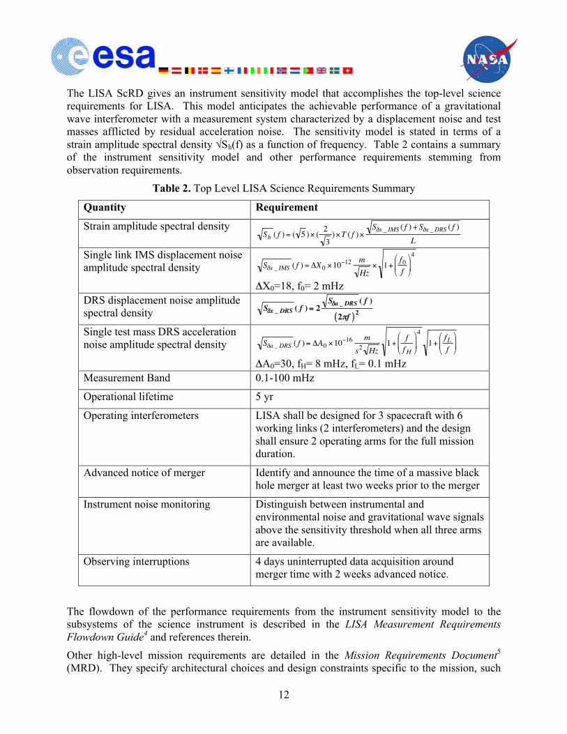
The LISA ScRD gives an instrument sensitivity model that accomplishes the top-level science requirements for LISA. This model anticipates the achievable performance of a gravitational wave interferometer with a measurement system characterized by a displacement noise and test masses afflicted by residual acceleration noise. The sensitivity model is stated in terms of a strain amplitude spectral density √Sh(f) as a function of frequency. Table 2 contains a summary of the instrument sensitivity model and other performance requirements stemming from observation requirements.

Table 2. Top Level LISA Science Requirements Summary

Quantity Requirement

Strain amplitude spectral density

€

Sh ( f ) = ( 5 )× ( 23)×T ( f )×

Sδx _ IMS ( f ) + Sδx _DRS ( f )L

Single link IMS displacement noise amplitude spectral density

€

Sδx _ IMS ( f ) = ΔX0 ×10−12 m

Hz× 1+

f0f

4

ΔX0=18, f0= 2 mHz DRS displacement noise amplitude spectral density

€

Sδx _ DRS ( f ) = 2Sδa _ DRS ( f )

2πf( )2

Single test mass DRS acceleration noise amplitude spectral density

€

Sδa _DRS ( f ) = ΔA0 ×10−16 m

s2 Hz1+

ff H

4

1+fLf

ΔA0=30, fH= 8 mHz, fL= 0.1 mHz Measurement Band 0.1-100 mHz

Operational lifetime 5 yr

Operating interferometers LISA shall be designed for 3 spacecraft with 6 working links (2 interferometers) and the design shall ensure 2 operating arms for the full mission duration.

Advanced notice of merger Identify and announce the time of a massive black hole merger at least two weeks prior to the merger

Instrument noise monitoring Distinguish between instrumental and environmental noise and gravitational wave signals above the sensitivity threshold when all three arms are available.

Observing interruptions 4 days uninterrupted data acquisition around merger time with 2 weeks advanced notice.

The flowdown of the performance requirements from the instrument sensitivity model to the subsystems of the science instrument is described in the LISA Measurement Requirements Flowdown Guide4 and references therein. Other high-level mission requirements are detailed in the Mission Requirements Document5 (MRD). They specify architectural choices and design constraints specific to the mission, such

13

as the number of spacecraft, the number and orientation of the arms, and the choice of laser interferometry as a measurement technique. These choices must be specified before the measurement system requirements can be fully defined.

14

4 Measurement Concept The description of the LISA mission concept begins with what is to be measured and the general concept for measuring it. The design concept is chosen to extract maximal information about astrophysical sources to answer questions about astrophysics and to test fundamental physics. The observation requirements in the previous section quantitatively connect the science objectives with the performance requirements on the conceptual design. The conceptual design in the following sections meets those performance requirements, with appropriate margin.

4.1 What’s to be measured Gravitational waves are a time-varying strain (∆L/L) in spacetime. They are predominantly quadrupolar, and consequently have two independent polarizations. Neither monopolar nor dipolar radiation are possible under General Relativity. Signal strength is determined by the time derivative of the mass quadrupole moment, thus favoring close binaries of compact objects.

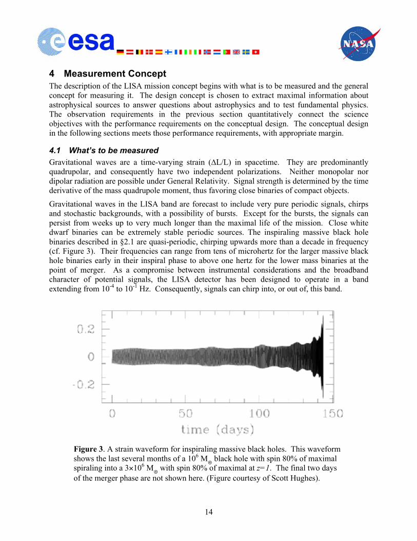
Gravitational waves in the LISA band are forecast to include very pure periodic signals, chirps and stochastic backgrounds, with a possibility of bursts. Except for the bursts, the signals can persist from weeks up to very much longer than the maximal life of the mission. Close white dwarf binaries can be extremely stable periodic sources. The inspiraling massive black hole binaries described in §2.1 are quasi-periodic, chirping upwards more than a decade in frequency (cf. Figure 3). Their frequencies can range from tens of microhertz for the larger massive black hole binaries early in their inspiral phase to above one hertz for the lower mass binaries at the point of merger. As a compromise between instrumental considerations and the broadband character of potential signals, the LISA detector has been designed to operate in a band extending from 10-4 to 10-1 Hz. Consequently, signals can chirp into, or out of, this band.

Figure 3. A strain waveform for inspiraling massive black holes. This waveform shows the last several months of a 106 M

black hole with spin 80% of maximal

spiraling into a 3×106 M

with spin 80% of maximal at z=1. The final two days of the merger phase are not shown here. (Figure courtesy of Scott Hughes).

15

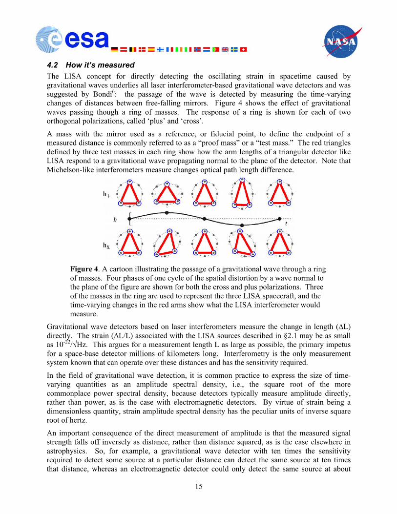
4.2 How it’s measured The LISA concept for directly detecting the oscillating strain in spacetime caused by gravitational waves underlies all laser interferometer-based gravitational wave detectors and was suggested by Bondi6: the passage of the wave is detected by measuring the time-varying changes of distances between free-falling mirrors. Figure 4 shows the effect of gravitational waves passing though a ring of masses. The response of a ring is shown for each of two orthogonal polarizations, called ‘plus’ and ‘cross’.

A mass with the mirror used as a reference, or fiducial point, to define the endpoint of a measured distance is commonly referred to as a “proof mass” or a “test mass.” The red triangles defined by three test masses in each ring show how the arm lengths of a triangular detector like LISA respond to a gravitational wave propagating normal to the plane of the detector. Note that Michelson-like interferometers measure changes optical path length difference.

Figure 4. A cartoon illustrating the passage of a gravitational wave through a ring of masses. Four phases of one cycle of the spatial distortion by a wave normal to the plane of the figure are shown for both the cross and plus polarizations. Three of the masses in the ring are used to represent the three LISA spacecraft, and the time-varying changes in the red arms show what the LISA interferometer would measure.

Gravitational wave detectors based on laser interferometers measure the change in length (∆L) directly. The strain (∆L/L) associated with the LISA sources described in §2.1 may be as small as 10-22/√Hz. This argues for a measurement length L as large as possible, the primary impetus for a space-base detector millions of kilometers long. Interferometry is the only measurement system known that can operate over these distances and has the sensitivity required.

In the field of gravitational wave detection, it is common practice to express the size of time-varying quantities as an amplitude spectral density, i.e., the square root of the more commonplace power spectral density, because detectors typically measure amplitude directly, rather than power, as is the case with electromagnetic detectors. By virtue of strain being a dimensionless quantity, strain amplitude spectral density has the peculiar units of inverse square root of hertz.

An important consequence of the direct measurement of amplitude is that the measured signal strength falls off inversely as distance, rather than distance squared, as is the case elsewhere in astrophysics. So, for example, a gravitational wave detector with ten times the sensitivity required to detect some source at a particular distance can detect the same source at ten times that distance, whereas an electromagnetic detector could only detect the same source at about

16

three times the distance. Where the space density of the source is constant, that implies a thousand times as many sources for the gravitational wave detector, and only 30 times as many for the electromagnetic detector. So although the extremely small strain makes gravitational wave detections inherently challenging, a robust detector can have an extraordinary reach.

So, the concept makes interferometric measurements between widely separated, free-falling masses carrying mirrors. ‘Free-falling’ or inertial masses are, by definition, undisturbed by forces comparable to gravitation. Consequently, the detector must be located in a very quiet environment to avoid disturbances to the test masses that result in time-varying movements that could be confused with the apparent displacements caused by gravitational radiation. A very stable, benign environment is possible in space with careful design choices for science instrumentation, spacecraft and orbits.

17

5 Science Instrumentation The science instrumentation of LISA fulfills the two main functions described in the previous section: (1) measure changes in the separation between test masses with the requisite displacement sensitivity and (2) limit disturbances to those test masses so that their spurious acceleration will not be confused with the gravitational wave signal. In the subsections that follow, a functional description of the science instrumentation is given, followed by a hardware description.

The basic mission concept consists of three identical spacecraft defining an equilateral triangle, 5 million kilometers on a side (see Figure 5). Each spacecraft houses two free-falling test masses that define the endpoints of the measured distances. Laser beams transit the triangle’s sides to monitor changes in their length. Although only two sides are necessary for an approximately equal-arm Michelson interferometer with a 60° included angle, the third side provides economical redundancy and simultaneous measurement of both wave polarizations. In this concept, the constellation of spacecraft is the science instrument. Spacecraft that are an integral part of the science instrumentation are sometimes called “sciencecraft.”

Figure 5. A constellation of three identical LISA spacecraft constitute the science instrument. There are six identical, send/receive laser ranging terminals with associated test masses and an intercomparison of signals at each apex.

The first function of the science instrumentation – measuring distance changes – is accomplished by continuous laser ranging between free-falling test masses using an interferometric readout to track variations in the round-trip travel time. The rate of arrival of 1 µm wavelength light must be measured to ~5 µcycle/√Hz. Thus, the measurement performance is characterized by a displacement sensitivity, or more properly a displacement amplitude spectral density. LISA

18

achieves its great strain sensitivity, in part, through a displacement sensitivity of 5×10-12 m/Hz over a pathlength of 5×109 m in a 1 second integration.

Many design features accomplish the second function, limiting unwanted disturbances. Foremost of these is the choice of unique heliocentric orbits (see Figure 6) with a relatively benign environment. Second, a “drag-free” control system limits the relative motion of the spacecraft with respect to the test masses. The free-falling test masses are enclosed in housings within the spacecraft. The spacecraft is held fixed with respect to the free-falling test masses by a control system that senses the position of the test masses within their housings and actuates the spacecraft propulsion system. Drag-free technology, pioneered for earth-orbiting satellites, allows the test masses to be shielded from external forces like the solar wind and photon pressure, and reduces the effects of force gradients arising in the spacecraft that act on the test masses. Care must also be taken to limit disturbances caused by the spacecraft. The residual acceleration noise, or more properly a residual acceleration amplitude spectral density, characterizes disturbance reduction.

Figure 6. The three LISA spacecraft orbit in an equilateral triangle. The red line shows the orbit of the orange spacecraft. The blue line shows the orbit of the Earth. The triangle is inclined 60° to the ecliptic plane. The sides of the triangle are 5×106 km, and the center follows the Earth in its orbit, ~20° behind (~50×106 km). The orbits are passive and require no stationkeeping.

The science instrumentation of LISA is most conveniently organized around the two functions described above. The Interferometer Measurement System (IMS) measures displacements and encompasses the equipment necessary to do that. The Disturbance Reduction System (DRS) includes the test masses and their associated equipment, the DRS control system and the micronewton thrusters that act as actuators. In addition, there are many features of the spacecraft and payload designs to limit thermal, magnetic, electrostatic, mechanical and self-gravity disturbances. The remainder of this section gives an overview of how each of these majors systems works and what equipment they require.

19

For a more detailed description of the science instrumentation than is given in the remainder of this section, see the Payload Preliminary Design Document7 and documents referenced therein. Documents describing the LISA Pathfinder mission are another important source of detailed technical information. LISA Pathfinder (LPF) is an ESA-led technology demonstration mission, scheduled for launch in 2011, and currently well into implementation. A great deal of practical engineering detail about LISA science instrumentation, particularly the DRS, can be found in the LPF documents. There is a concise overview, 8 and a more comprehensive description,9 as well a large number of project technical documents.

5.1 Interferometry The Interferometry Measurement System makes a 3-part distance measurement. There are two “short arms” which measure changes in the distance between the free-falling test mass and a reference point on the spacecraft at either end, and one “long arm” operating between the reference points on spacecraft. Both short arm measurements are performed by polarizing, heterodyne interferometers. The long arm measurement is performed with an active transponder scheme, analogous to a police radar gun. A ‘master’ laser beam is sent from one spacecraft to another, and the ‘slave’ laser on the remote spacecraft is phase-locked to the weak incoming beam and transmits back a full power beam to original spacecraft. The phase of that beam is compared to phase of the master laser by ‘beating’ the weak incoming beam with the local laser. The time-varying optical path caused by a gravitational wave impresses a phase modulation on the returning beam that shows up in the beat signal. The high displacement sensitivity makes this more difficult for several reasons: the round-trip light time is about 32 seconds; the beating of the return signal compares the laser frequency noise at the instant of measurement with that of 32 seconds previous; the natural laser frequency noise is much greater than the phase modulation from the gravitational wave (i.e., ∆f/f >> 10-22/√Hz); and the clock noise used for the phase measurement is similarly too great. Design features in the measurement system or noise subtraction algorithms in data analysis overcome each of these difficulties.

5.1.1 What it does The major functions of the interferometry system are the generation of appropriate laser beams, laser power and frequency stabilization, beam steering and combining for both short- and long-arm interferometry, beam pointing, ranging, fringe detection, timing and phase measurement. Each of these functions is addressed in turn below.

5.1.1.1 Lasers The interferometry concept requires two laser sources in each spacecraft with ample power for both the two beams transmitted to the far spacecraft, the short-arm interferometry and intercomparison with each other. These lasers must have intrinsically stable power and frequency, and be further stabilized to a high degree in both parameters. The general concept is to have the two lasers in each spacecraft associated with one long arm, and to have a back fiber link connecting them. The heterodyne interferometer that performs the short-arm measurement uses a small amount of light from each of these. One of the six lasers in the constellation would be the master, and the other five would be phase-locked to it through a long arm and/or a back

20

link fiber. Each of the phase-locked lasers would be offset by a programmable offset frequency, plus the Doppler frequency associated with a changing long arm, if there is one.

5.1.1.2 Laser Frequency Noise Laser frequency noise will swamp the gravitational wave signal by many orders of magnitude, if the natural frequency noise in candidate lasers is present. However, the laser frequency noise is reduced to a minor contributor to the error budget by three techniques. First, the master laser frequency is pre-stabilized with a passive optical cavity made of an ultra-stable material. Second, the master is further stabilized to a sum of the long arms, because of their great stability, particularly at low frequency. Note that the gravitational wave signal is in the difference of the long arms because of the quadrupolar nature of gravitational waves. Finally, the residual laser frequency noise in the acquired signal is cancelled through a post-processing algorithm known as Time Delay Interferometry (TDI). Although TDI is a data processing algorithm rather than a part of the flights system, it is important to understand its benefit in the context of the Interferometry Measurement System. TDI effectively simulates a generalized equal-arm Michelson interferometer. Through the natural cancellation of frequency noise by an equal-arm interferometer, Michelson was able to make measurements only a decade less precise than LISA needs, using white light, let alone noisy lasers. Despite having slightly unequal and changing length arms owing to the spacecraft orbits, the LISA concept achieves a generalized “white-light fringe” condition by recombining the beams from different arms digitally with the appropriate phase delay. This is made possible because the incoming beams measuring the two arms are not combined at a beamsplitter, as in the classic Michelson interferometer. Rather each one is combined at a beamsplitter with its originating laser, and the two lasers are separately compared via the back link optical fiber. At the start of the data analysis, the two time series from the long arms are combined with a time shift to achieve the equal path length condition that nominally cancels all frequency noise. TDI is described in more detail in LISA Data Analysis Status10 and the references therein.

5.1.1.3 Beam Steering and Combination The obvious function in any interferometer is the steering and combination of beams with mirrors, beamsplitters, polarizers, fibers and mode matching optics. The LISA interferometry has a few special needs:

• The short arm interferometer must reflect a beam off of a free-falling, gold-coated test mass. Attention must be paid to the geometric interface between the test mass and the interferometer.

• To reduce diffraction losses over the long arm and to collect more returning light, the beam is expanded/compressed by a couple of orders of magnitude.

• A beam must be brought to a CCD for initial acquisition of pointing of the long-arm optical paths.

• Polarization is used to separate incoming and outgoing beams in the long-arm interferometer and beams onto and off of the test mass in the short-arm interferometer.

• All critical components are bonded onto an optical bench of ultra-stable material

There are three required beam pointings in the LISA interferometry concept:

21

• The beam transmitted over the long arm must be pointed towards the distant spacecraft. As the constellation orbits about the Sun, orbital mechanics imposes a small, slow change in the triangular geometry, wherein the included angles change ±~1° (cf §7.1). The LISA concept addresses this by moving the optical assemblies that constitute the transmit/receive terminal (i.e., test mass assembly, optical bench and telescope).

• Because of the light transit time (i.e., 16 s), the distant spacecraft moves an appreciable angular distance from where it was when the incoming beam left it to where it will be when the transmitted beam arrives at it. The transmit beam must be pointed ahead of the received beam by a few arc seconds that again varies slightly over the course of a year.

• The test masses are free-falling, but only in one degree-of-freedom, along the measurement direction. In the other 5 degrees-of freedom, they must be controlled. This is discussed further below in §5.2.1. The tip and tilt of the test mass amounts to the alignment of the free-falling mirror with the rest of the interferometer. The IMS measures test mass orientation so that the test mass mirror can be kept in alignment with the optics.

5.1.1.4 Ranging TDI requires knowledge of the distance between the spacecraft to tens of meters. This can be readily accomplished by a ranging system based on a laser sideband. This absolute distance measurement is many orders of magnitude less precise than the measurement of time-varying displacement needed for the main science measurement.

5.1.1.5 Photodetectors When two light beams are superposed to produce fringes, the beat signal is captured by photodetectors. The photoreceivers for the long-arm interferometers have to accommodate the beat of the weak incoming signal (>108 photons/sec) against the strong local reference laser. The beat frequencies, given by inter-spacecraft Doppler, can range up to 20 MHz. Many of the LISA photoreceivers are quadrant detectors to produce angular information from differential phase measurements.

5.1.1.6 Phase Measurement Phase measurement at the level of 10-5 cycles/√Hz is a critical function in the IMS. Each photoreceiver channel requires a phasemeter channel to measure variations in the arrival rate of fringes. The phasemeter must also extract ranging, clock and telemetry information from laser sidebands. In the case of fringe signals for laser phase-locking loops, the phasemeter must provide a high frequency error signal for controlling the laser frequency.

5.1.1.7 Timing Timing is the final function of the IMS to be discussed here. An ultra-stable oscillator is necessary for data sampling and time stamping. As with the laser, readily available, flight-qualified oscillators have more frequency noise than the LISA concept can tolerate, if used without correction. However, by imposing a signal derived from each of the clocks on long-path laser beams, TDI can be used to remove the clock frequency noise from the final data just as the laser frequency noise is removed.10

22

5.1.2 What it takes to do it The previous section described the major functions of the interferometry in the LISA. This section describes the equipment to carry out those functions. This concept document must necessarily give only an overview of this equipment. For example, features associated with redundancy are generally not described here. Much more detailed descriptions, functional and performance requirements and analyses can be found in the Payload Preliminary Design Description7 and its references.

The interferometry equipment is organized into two identical moving optical assemblies and the avionics boxes housing electronics and laser subsystems. The moving optical assemblies consist of a telescope, an optical bench, and Gravitational Reference Sensor (GRS). See Figure 7. Each of the two moving optical assemblies in a spacecraft acts as a transmit/receive terminal for a measured arm. Each is mounted on flexural hinges and pointed by a precision mechanism to accommodate the annual variation in the angle between the directions to the distant spacecraft.

Figure 7. Moving optical assembly. The off-axis telescope, optical bench (OB) and Gravitational Reference Sensor (GRS) Head are shown.

5.1.2.1 Laser subsystem The baseline architecture for the laser subsystem is a master oscillator, fiber-amplifier. The master oscillator is expected to be a non-planar ring-oscillator (NPRO) type, pumped by fiber-coupled diodes, commonplace in commercial and space applications (see Figure 8). The frequency of these lasers is tunable by both slow thermal and rapid PZT actuators. The laser is also power stabilized. Fiber amplifiers add very little phase noise, and are efficient, robust and capable of much higher power output than is needed. Important characteristics are:

• 25 mW, diode-pumped Nd:YAG solid-state master oscillator • 2 W, Yb-doped fiber amplifier

• 8 GHz, fiber-based, electro-optic phase modulator • Fully redundant, fiber-coupled

23

Figure 8. Laser subsystem components. The left-hand photo shows a qualification model of the LISA Pathfinder laser, suitable as the master oscillator for LISA. The center photo shows an engineering model of a fiber amplifier module. The right-hand photo shows a fiber-based electro-optic phase modulator that can meet LISA frequency and power requirements.

5.1.2.2 Laser frequency control subsystem The architecture of the laser frequency control subsystem is still under consideration. There are multiple options for meeting the requirements, and the choices are between economy and performance margin. As described in §5.1.1.2, three strategies will be employed:

• There are multiple methodologies for laser frequency pre-stabilization. Pound-Drever-Hall sideband-locking to a reference cavity (see Figure 9) is the most effective, reaching 30 Hz/√Hz at 1 mHz. This technique locks a laser sideband frequency to a resonant optical cavity based on an ultra-stable material, such as ULE™ or Zerodur.™ The use of a sideband introduces a programmable offset frequency to accommodate arm-locking. Alternatively, this could be done with a variable cavity using a piezoelectric actuator, or an auxiliary interferometer with unequal arms. These techniques are well known in laser metrology.

• Arm-locking uses a sum of the arm length measurements to derive an error signal for laser frequency control.

• TDI is applied in post-processing, but requires moderate precision knowledge of the long path lengths and accurate timing of the sampling.

24

Figure 9. Optical reference cavity inside multiple thermal shields. This cavity meets LISA prestabilization requirements using Pound-Drever-Hall sideband-locking, despite a thermal environment that is not as stable as the LISA environment is expected to be.

5.1.2.3 Optical bench Figure 10 shows a realistic layout of the optical bench, the essential constituents of which are:

• A structural baseplate of an ultra-stable material, such as Zerodur, to provide geometric stability,

• Hydroxy-catalysis bonding of optical components to the baseplate for strength, stability and reliability,

• Fiber couplers to bring beams from the laser subsystem into the optical layout, and exchange beams between optical assemblies,

• Turning mirrors, beamsplitters, polarizers, baffles, beam dumps, etc. mounted on the baseplate,

• A point-ahead mechanism to maintain the small, variable angle between incoming and outgoing beams,

• Photoreceivers for recording the beat signals of combined beams, often quadrant detectors to also provide differential beam pointing,

• CCD camera for boresight acquisition of the distant spacecraft.

25

Figure 10. A practical layout of the optical bench mounted in a composite support ring.

Figure 11 shows a photograph of a prototype optical bench developed for LISA Pathfinder that incorporates many features of the LISA optical bench, notably the short-arm interferometer. The flight model of this interferometer has exceeded the measurement sensitivity required of the LISA short-arm interferometer.

Figure 11. Photograph of a prototype optical bench showing a Zerodur base and hydroxy-catalysis bonded components. This prototype was developed for ESA’s LISA Pathfinder mission, and is very similar to the LISA short-arm interferometer.

26

5.1.2.4 Telescope Each moving optical assembly has a transmit/receive telescope for coupling between the optical bench and the long-arm between spacecraft. The telescope reduces diffraction spreading of the transmitted beam and matches a large receiving area to the 5 mm optical laser beam on the optical bench is expanded through an afocal telescope. The telescope also compresses the incoming beam from the larger collecting area to a smaller beam size on the optical bench. The current design is an f/1.5, 400 mm diameter, off-axis variant of the Cassegrain, called a Schiefspiegler, with a transmissive ocular. The major considerations are stability of the wavefront and optical pathlength, low stray light, and the positioning of entrance and exit pupils. The field of view must be able to accommodate the point-ahead angle of a few arc seconds. In the benign environment of the LISA spacecraft, this design can be realized with available materials and construction methods. Detailed requirements and a design prescription can be found in the Payload Preliminary Description.7

5.1.2.5 Pointing mechanisms Two pointing mechanisms are required in the science instrument. One points the optical assembly (cf. Figure 7) to keep the entire transmit/receive terminal pointed at the distant spacecraft as the included angle of the constellation’s triangle varies ±1.5° with a one-year period owing to natural orbital effects. The optical assembly is mounted on flexural pivots, and a actuator mechanism acts on the inboard end to swivel the entire assembly. The baseline concept for the actuator is a piezoelectric crawling mechanism such as a NEXLINE piezomotor. Redundancy is achieved through one mechanism on each optical assembly and the attitude control of the spacecraft.

The second required mechanism compensates for the slowly varying point-ahead angle. Because the distance spacecraft moves through an appreciable apparent angle during the round-trip light travel time, the transmitted beam must be sent in a direction different from the received beam by a few arc seconds. The tiltable mirror is mounted on the optical bench. The stability requirements, especially the limit on piston motion, are stringent. A candidate design based on elastic Haberland hinges and an integrated capacitance sensor is being prototyped.

5.1.2.6 Photoreceivers [This section needs to be re-written to describe the hardware, not the functions.] Optical heterodyne signals for long- and short-arm interferometers are detected with quadrant photodiodes to enable differential wavefront sensing. In the case of the short-arm interferometer, the tip, tilt and piston information is used by the DRS control system, as well as the science measurement. InGaAs photodiodes with integrated transimpedance amplifiers can meet the requirements for bandwidth dictated by inter-spacecraft Doppler (<20 MHz) and the requirements for intensity and phase noise. A modest (~640x512 pixels) CCD image sensor is also required for the initial acquisition process. It must have sufficient field of view to accommodate the initial pointing error and sufficient compatible with the field of view of the science quadrant photodetector.

5.1.2.7 Phase measurement subsystem [This section needs to be re-written to describe the hardware, not the functions.]

27

The essential measurement of the science instrument is a phase measurement of the electrical signal from a photoreceiver channel. Gravitational waves manifest as a phase modulation of a beat signal at millihertz frequencies. In the case of a phase-locked laser, the phase measurement serves as a 50 kW error signal for the laser frequency control. The phase differences between different elements of a quadrant photodiode are used to monitor the angle between interfering optical beams and provide error signals to the DRS control system for telescope pointing and test mass attitude control. The phasemeter will have 58 analog channels, and 32 phase measurement channels.

The Phase Measurement Subsystem incorporates a number of other functions: an ultra-stable oscillator (USO), programmable frequency sources, time stamping, and encoding/decoding of data and ranging information onto/off of the inter-spacecraft optical link. The USO acts as a master frequency for time-keeping, phase measurement and digital frequency synthesis of various modulation frequencies.

5.2 Disturbance Reduction The Disturbance Reduction System (DRS) is a collection of design features chosen to reduce the residual disturbances on the test mass that would otherwise look like gravitational waves. This is largely accomplished by having a free-falling test mass that the spacecraft follows with “drag-free” technology. A drag-free spacecraft is one which is forced to follow a protected reference mass. A DRS control system has a means for sensing the location and orientation of a reference mass, a propulsion system and an implementation of control laws for transforming an error signal from the sensors into propulsion commands to hold the spacecraft fixed with respect to the reference mass. The terminology stems from application to earth-orbiting satellites, dating back to the 1970’s, to mitigate the drag of the residual atmosphere.

LISA uses drag-free technology in part to isolate the test mass from the Sun’s radiation pressure and the solar wind, but more importantly to hold the spacecraft fixed with respect to the test mass. This keeps the relative motion of the test mass and spacecraft from giving rise to time-varying forces owing to force gradients arising in the spacecraft and acting on the test mass. In reality, the LISA test masses only fall freely along the direction of their respective measured arms; they are forced to follow the spacecraft in the other five degrees of freedom. This is how a single spacecraft can follow two test masses at one time. The other disturbance reduction features mitigate unwanted forces from acting on the test masses. Forces of magnetic, electrostatic, gravitational, thermal and material origin are reduced to acceptable levels by careful choices of materials and/or geometry in the scientific equipment, the surrounding spacecraft, and even the orbits. All known interactions are modeled to support an error allocation and current best estimates; extensive laboratory measurements are made to validate the models and search for unknown interactions.

5.2.1 What it does The test masses are the realization of Bondi’s free-falling mirrors; their reflecting surfaces define the measured distances. Their trajectory – at least along the measured direction – is meant to be a geodesic. The goal of the DRS is to reduce all test mass disturbances so that their combined resultant motions are much less than the apparent motions caused by the expected gravitational-wave strain. The main functional components are the test mass subsystem, the spacecraft

28

propulsion system, the DRS control laws, and assorted design features of the payload and spacecraft.

5.2.1.1 Gravitational Reference Sensor The test mass is housed in a subassembly, called the Gravitational Reference Sensor (GRS), that accomplishes several functions: shielding the mass from magnetic and thermal noises, sensing the position and orientation of the mass, applying appropriate forces to the mass in six degrees of freedom, sensing and discharging the test mass and housing to compensate for cosmic ray charging, enclosing the mass in a high vacuum environment, and caging the mass during launch so that it can be released with a very low velocity on the operational orbit. See Figure 12.

Figure 12. Examples of disturbances. Two test masses (gold) are notionally shown inside their housings within the spacecraft. Disturbances can arise from the external environment, the interface to the interferometry, the spacecraft bus, the payload and even the gap between the test masses and their housings.

29

The test mass is more than a free-falling mirror. As the measurement fiducial, the test mass is a critical interface with the optical system; its geometry, position and orientation profoundly affect the interferometry. The short-arm interferometer likewise affects the test mass through shot noise and dissipation.

The test mass will be subjected to many residual forces. Consequently, high density will minimize the resulting acceleration. Density inhomogeneities will affect the location of its center of mass. Low magnetic susceptibility will reduce the effect of spurious magnetic fields. The surface, at least, should be an excellent conductor, and have minimal variations in its work function (i.e., patch effect). Excellent thermal conductivity will reduce spurious forces caused by temperature gradients, such as the thermal radiation pressure and residual gas. A complete enumeration of the factors affecting the test mass is too lengthy for this document; only prominent examples have been given here.

The housing surrounding the test mass provides a reference frame from which to measure the position and orientation of the test mass with respect to the spacecraft. It also serves as a structure from which to apply a force to the test mass, without mechanical contact. During normal operation of the LISA DRS control system, the test mass is controlled in 5 degrees of freedom, and is free-falling in the measurement direction. In some other modes, it may be necessary to “cage” the test mass, necessitating the application of force in the measurement direction. The housing must also serve to reduce unwanted disturbances by high thermal conductivity, high heat capacity, very low residual magnetism. One very important characteristic is the gap between the housing and the test mass. A large gap serves to reduce several types of disturbances, but the sensitivity of capacitive sensing and the available forcing authority, say from electrostatic forcing is also reduced. The sensing will impose back-action noise on the test mass and create a virtual spring coupling residual spacecraft motion to the test mass. Cosmic rays impacting the housing and the test mass will deposit charge on one or the other components that will give rise to electrostatic and Lorentz forces. The GRS must support charge control, that is, sensing and non-contacting discharge of the test mass and housing.

The GRS supports three other seemingly less important functions: a vacuum system to protect the test mass from contamination and residual gas pressure, a caging system to hold the test mass during launch and trim masses to balance the residual self-gravity and gravity gradient of the surrounding equipment. The caging function includes the challenging requirement of releasing the test mass with extremely low velocity after holding it with very high force. The low-velocity arises because of the low force authority available in non-contacting forcers.

5.2.1.2 Microthrusters Drag-free control of the spacecraft requires a propulsion system with appropriately low thrust and low thrust noise. For LISA spacecraft, there is a constant ~9 micronewton (µN) force from solar photon pressure that must be countered. Very low thrust, low noise (<0.1 µN/√Hz) propulsion with proportional control is needed for drag-free control. In the usual science operations mode, the GRS will sense a position error as the spacecraft drifts away from the test mass, and the controller will command the spacecraft thrusters to make the spacecraft follow the test mass with the requisite tolerance. Five years of science operations lead to a 44,000 hr lifetime requirement, which can be significant for the candidate technologies. A high specific

30

impulse (i.e., thrust per unit mass of propellant) and a propellant that does not slosh are also desirable characteristics.

The microthrusters are the only propulsion system on the spacecraft after the propulsion module used to get the science craft to the operational orbit separates. Consequently, in addition to the science mode requirements, they must also serve the demands of tip-off/de-spin, initial acquisition of the array, and safe modes. Some of these considerations set the desirable maximum thrust around 30 µN.

5.2.1.3 DRS control laws The DRS control system governs the orientation of the spacecraft, the position of the spacecraft relative to the two test masses, the orientation of the two test masses, the position of the test masses relative to their housings in degrees of freedom (DoF) orthogonal to their respective measurement directions, the articulation angle between the two telescopes and the point-ahead angle for both measurement arms. While, practically, there will be several modes for safe hold and acquisition, this section only describes the science operations mode. The DRS control laws will be implemented in an appropriate computer. The sensor input will be:

• Test mass orientation and position input from the short-arm interferometers, • Test mass orientation and position input from the capacitance sensors in the GRS,

• Beam tip/tilt from the long-arm interferometers • Pointing information from the distant spacecraft

The controller output commands will go to: • Electrostatic forcing of test mass orientation and position in the degrees of freedom other

than the measurement directions, • Micronewton thrusters controlling spacecraft orientation and position,

• Pointing actuator on one telescope (the other is fixed with respect to the spacecraft) • Point-ahead actuator on the optical bench.

This 19 DoF controller needs a 10 Hz bandwidth and a latency less than 300 milliseconds. While not functionally a part of the DRS control system, an AC signal must be added to the electrostatic forcing signal going to transverse electrodes and demodulated from the associated capacitance sensors to sense the charge.

5.2.1.4 Payload and spacecraft features The payload and spacecraft must shield the test masses from disturbance, and must not contribute any substantial disturbance themselves. Generally, the residual forces acting on the test masses should be very low, and have very little variability in the measurement bandwidth. Further, very low force gradients are desirable because the noise in the drag-free control system will cause those gradients to act like time-varying forces on the test masses producing motions like gravitational waves. Thermal, magnetic, electrostatic and gravitational disturbances can all give rise to forces on the test masses.

31

Thermal disturbances illustrate how the spacecraft and payload shield the test masses and how they also harbor sources of thermal noise. Fifty million kilometers behind the Earth, the dominant external thermal noise source is the variability in solar heating. The orbits of the spacecraft (see §7.1 below) are such that the Sun shines on the top of the spacecraft at a 30° angle to the normal at all times. Variability comes about because of changing absorptivity of the spacecraft, variability in the solar constant from supergranules and solar oscillations and in the small eccentricity of the annual orbit. The spacecraft and payload design must provide multiple stages of passive thermal isolation to reduce thermal variability at the test mass, and on the optical bench. The GRS electrode housing and vacuum container are constructed to reduce gradients across the test mass. Thermal variability and/or gradients at the test mass can induce noise from asymmetric thermal radiation, asymmetric recoil of residual gas around the test mass, and asymmetric outgassing. Eccentricity effects are the largest, but are three decades outside the measurement band. All of the avionics boxes threaten thermal disturbances of local origin. Passive thermal design and selective power dissipation control can adequately mitigate these disturbances. An extensive itemization of the thermal, magnetic, electrostatic and gravitation disturbances and their coupling to the test masses is not possible here. Disturbance reduction requirements can be satisfied with conventional but careful thermal engineering and magnetic cleanliness. Electrostatic and gravitational effects require unusual, but not extraordinary, design features like charge control and gravitational balance. Commonplace materials and construction methods are adequate for all but the equipment within centimeters of the test masses. A requirements flow down can be found in LISA Measurement Requirements Flowdown Guide.4 A detailed catalog of disturbances can be found in LISA DRS Acceleration Noise Budget.11

5.2.2 What it takes to do it

5.2.2.1 Gravitational Reference Sensor The GRS is arguably the most unique and challenging subsystem in the scientific instrumentation for LISA. The LISA design is derived from a line of space accelerometers developed by ONERA, a CNES research lab, and most recently flown on the Gravity Recovery and Climate Experiment (GRACE) mission. To retire the technical risks, the LISA design has already been developed for the LISA Pathfinder mission and is now in flight implementation.8,9 That design is shown in Figure 13.

The test mass is a 1.96 kg cube, 46 mm on a side, made of a 73/27% platinum/gold alloy. This material has very low magnetic susceptibility (~10-5) to minimize magnetic disturbances, very high density (~20 kg/m3) to limit motion from all disturbances and excellent thermal properties to limit gradients and thermal variability. It is gold-coated for maximum electrical conductivity and minimal work function variations. The electrode housing is a hollow cubical box enclosing the test mass. It is made of molybdenum, with gold-coated sapphire electrodes set in the interior walls. The size of the electrode housing is chosen to leave a 4 mm gap between the test mass and its surroundings. This gap is two orders of magnitude larger than the ONERA accelerometers, or recent drag-free missions like GP-B. It was chosen to reduce noise sources such as work function variations while still meeting the capacitive sensing requirement over the measurement.

32

Figure 13. Gravitational Reference Sensor. A cross-section drawing shows a test mass, its electrode housing, the caging mechanism, the charge management system, and the front-end electronics for capacitive sensing and forcing. Engineering models of the subsystems from LISA Pathfinder are shown in the photographs.

The Front End Electronics employs a capacitive bridge using electrodes on opposing faces of the test mass to sense changes in its position or orientation. Note that the position and orientation sensing is augmented by the interferometric piston, tip and tilt measurements made by the short-arm interferometer. The electronics is also used to apply forces to the test mass for the drag-free control system and a rotational stimulus for charge sensing.

33

Charge control is accomplished by UV photo-dissociation from the gold-coated surfaces. The light is brought into the housing via optical fibers and shown on either the test mass of the housing wall depending on the sign of the discharge needed. To prevent damage from the ~50 grms launch vibrations, the test mass must be caged with a force of ~2000 N during launch and then released within a 200 µ error box with a residual velocity of less than 5 x 10-6 m/s2. The LPF design has a three stage actuator consisting of a hydraulic piston to provide the launch lock, a second stage actuator to break the first stage adhesion and provide the positioning, and a third stage to break the second stage adhesion and release the mass with the required accuracy. Finally, the GRS is housed in a titanium vacuum vessel for magnetic cleanliness. A getter pump will maintain the vacuum below 10-6 Pa for the life of the mission. The vacuum system design will accommodate trim masses for reducing the self-gravity field and its gradient.

5.2.2.2 Microthrusters Three different electric propulsion systems are currently being developed for LISA; they are based on the electro-spray of nano-droplets or metal ions. Two designs are based on the Field Emission Electric Propulsion (FEEP) technology wherein metal ions are extracted from the liquid phase and accelerated by an electric potential. One of those two emits cesium from a slit, and the other emits indium from an array of needles. The third design, called colloid micronewton thrusters (CMNT), emits a very fine spray of a highly conductive liquid from an array of needles. The cesium slit-FEEP thrusters and the CMNTs will be flown on LISA Pathfinder. The indium needle-FEEP thrusters will continue to be developed on ground as a backup. One of these technologies will be selected for LISA after LPF and on-going ground-based lifetime testing are complete. All three technologies have been shown to satisfy LISA performance requirements. Lifetime is the primary focus of microthrusters development. In the interim, the baseline architecture of LISA accounts for the higher mass and power requirements of the CMNTs.

The underlying concept of all these technologies is shown in Figure 14. The propellant is brought to an “emitter” in the liquid state, and then electrostatically drawn out into a Taylor cone and a jet, and then atomized and accelerated, a process known as electro-spray. The geometry of the emitter is chosen to accentuate the effect of the electric field on the surface of the liquid. The spray consists of metal ions in the case of the liquid-metal FEEP, and nano-droplets in the case of the colloid fluid. An electron source neutralizes the exhaust plume, and, in effect, the entire spacecraft. Generally, proportional control of the thrust is achieved by manipulating voltage and current, though the CMNTs also have a micro-valve in the propellant supply line.

The propellant, the manner of propellant supply and the geometry of the emitter distinguish the three technologies. All three technologies would have three clusters of four active thrusters on the LISA spacecraft bus; six of the twelve thrusters must operate continuously after separation from the propulsion modules, about 10 years for an extended mission. The entire propulsion subsystem is redundant.

34

Figure 14. Conceptual depiction of electro-spray thrusters. The liquid propellant (yellow) is conveyed to an “emitter” and “extracted” as a fine spray by an electrostatic potential. The exhaust plume is neutralized by a cathode (blue). Proportional thrust control is achieved via the voltage and current of the emitter. See text for further explanation.

The Busek Company in Natick, MA manufactures colloid micronewton thrusters (see Figure 15). The propellant is a highly conductive liquid stored in a pressurized reservoir. The liquid is supplied to a manifold in the thruster heads through a precision micro-valve, and drawn by capillary action up hollow needles arranged in a 3x3 array. The liquid is converted to a spray of nano-droplets by a high voltage between the needle tip and an extraction electrode. Proportional thrust control is effected through voltage and current controls; propellant supply rate is controlled by the micro-valve.

35

Figure 15. Colloid micronewton thrusters. The two flight-model clusters for LPF, left, have completed all subsystem-level testing and are awaiting delivery for LPF integration. The 3x3 arrangement of needles can be seen in the prototype thruster head on the right.

ALTA, S.p.A in Italy manufactures cesium slit-FEEP thrusters (see Figure 16). The cesium propellant is housed in the thruster head. Because of the very high specific impulse, only ~10 gm of cesium are needed per thruster head for the 8.5 yr extended lifetime of the mission. It is heated to the melting point and supplied to a 10 x 0.001 mm metal slit by capillary action. A few kilovolts are sufficient to raise Taylor cones on the surface of the cesium, pulling off ions and accelerating them. Multiple extraction sites form along the slit, and the maximum thrust is set by the slit length. The slot that acts as the accelerating electrode can be seen in the right-hand thruster in the left-hand photo. Each thruster is covered by a lid, seen opened on the left-hand thruster in the left hand photo, to prevent oxidation of the cesium. The lids are opened after the spacecraft leaves the Earth’s atmosphere and before operation.

36

Figure 16. Clusters of cesium slit-FEEP microthrusters. The left-hand photograph shows the LPF flight spare. The right-hand photograph shows the engineering model (EM) on the LPF spacecraft for system level acoustic testing. The EM has one thruster head (right) and three mass dummies. See text for additional details.

The Austrian Research Centre (ARC) in Siebersdorf manufactures the indium needle-FEEP thrusters (see Figure 17). The indium propellant is melted and drawn up roughened needles by surface tension. A high voltage is applied by an extractor electrode to form Taylor cones, a jet, and an electro-spray of metal ions. The needles also have accelerator and beam-focusing electrodes. Liquid metal ion sources, based on the same technology, have flown as charge control devices on the GEOTAIL and CLUSTER missions.

Figure 17. Clusters of indium needle-FEEP microthrusters. The photograph on the left shows an array of needle-FEEP thrusters firing during a lifetime test. The photograph on the right photo shows a prototype cluster. See text for additional information.

5.2.2.3 DRS control laws The DRS control laws control: (1) the relative positions and orientations of the spacecraft and test masses, (2) telescope pointing, and (3) the point-ahead actuator. During science operations the test masses are allowed to fall freely along their associated measurement directions. In

37

standby modes, the DRS control laws electrostatically cage the test masses. In the acquisition phase, the DRS control laws would point the spacecraft at each other for laser acquisition and coordinate laser tuning to acquire a suitable heterodyne beat frequency. The multiple-input-multiple-output control system have been designed using conventional servo control methods, and will be implemented as software modules on a flight computer. Figure 18 shows a notional flowchart of the control system. Numerical models, frequency domain analysis, and time domain simulations with all three spacecraft by both NASA and ESA engineers have shown that the drag-free performance requirements can be met with sensor and actuator performance as currently understood.

Figure 18. DRS control system. See text for discussion.

The DRS control system uses information from many sensors to control the relative positions and orientations of the test masses and spacecraft, and the angle between the telescopes. The use of quadrant photoreceivers throughout the IMS enables angular sensing through phase differences between the quadrants, as well as the usual translation information. The long-arm interferometers measure local optical system pointing with respect to the incoming beam, and the short-arm interferometers provide high precision information on test mass translation along, and tip/tilt about, their respective measurement directions. Consequently, the DRS control system must process phase measurements from individual photoreceiver quadrants for translation and angle inputs. The capacitance sensors in the GRS (cf §5.2.1.1) provide information about test mass translation and orientation in the degrees of freedom not sampled interferometrically. The control system

38

will get this information from the GRS Front End Electronics. Two star trackers on the spacecraft bus provide coarse attitude determination during initial acquisition of beams between spacecraft. The DRS control system commands many actuators. The test mass attitudes and positions with respect to their reference electrode housings are commanded through voltages on the electrode plates. Hence the DRS control system must send commands to the GRS Front End Electronics. It commands 12 micronewton thrusters to control spacecraft attitude and position relative to the test masses. And, it commands the mechanism pointing one optical assembly and the point-ahead mechanisms for both optical assemblies (see §5.1.2.5). The DRS control system must operate over a frequency band comparable to the measurement bandwidth of LISA, 0.03 to 100 mHz. Further, it must ensure that no out-of-band effects, such as dynamic range limits, affect the in-band performance.

After the three LISA spacecraft are initially injected into their operational orbits, and the propulsion modules are separated, all six long-arm interferometer links must be established by pointing their optical assemblies at each other and tuning their lasers to get an acceptable beat frequency. [N.B. The term ‘link’ denotes a one-way measurement along one side of the triangular formation.] The acquisition is complicated because, prior to link establishment, the spacecraft can only be coordinated by ground control.

At one time, this acquisition was thought to be a driving requirement for the DRS control system because of the final pointing precision needed by each of the six telescopes was a thousand times better than the pointing available from common star trackers. It is also impossible to test the process with final flight hardware under realistic conditions. A substantial effort went into modeling and analyzing two different methods: de-focus and scanning.12,13 Both have been shown to be feasible, and can be implemented with the baseline equipment. The defocus method is substantially faster and somewhat more robust. The acquisition sequence using the defocus method can be summarized as follows: All six telescopes are coarsely pointed with knowledge from DSN spacecraft tracking and the star trackers. All spacecraft are set to follow a blend of star tracker and GRS information. To start, two incoming links to one spacecraft are acquired, and then one beam between the other two spacecraft is acquired. To acquire a link, the transmitter defocuses its telescope to spread its beam by a factor of 7.5. The receiving optical assembly on the distant spacecraft detects the incoming laser beam on its acquisition CCD, and points its telescope toward the distant spacecraft by centering the beam centroid on its CCD. This is repeated for the second and third links. Then the three return links are established in the same manner. Note that the original beams need to be suppressed briefly to prevent scattered light from the local laser from flooding the CCD, but they can be quickly re-acquired without repeating the acquisition. After the bidirectional beams are established, then the telescopes can be re-focused, and the pointing further optimized with the intensity on the quadrant cells, which also requires briefly turning off the local laser. Once the constellation pointing is established with incoherent light, the lasers must be tuned to achieve acceptable beat frequencies (<20 MHz) for the interferometric acquisition. Initially, all laser frequencies are adjusted to the best estimate according to the frequency plan, ground tuning calibration and the inter-spacecraft Doppler shifts known from ground-tracking. For any link

39

where the beat frequency is out of range, the local laser can be adjusted to get the desired beat frequency, at which point the beat frequency for the opposite going link is also set. This process is repeated as necessary to acquire interferometric lock. Then the frequencies need to be systematically migrated so that the beat notes between lasers in the same spacecraft matches the frequency plan, including the offset phase-locking (see §5.1.1.1). Once interferometric lock is established throughout the constellation, the phase difference between halves of the quadrant photoreceivers is used to achieve the final pointing accuracy needed for science operations. The scanning method simply scans over the uncertainty cone instead of de-focusing. At each scan location, the transmitter waits briefly for the receiver to turn on, if it has detected the incoming beam. If not, the scan continues until the correct pointing direction is found. Otherwise the acquisition process proceeds as with the de-focus method.

5.2.2.4 Payload and spacecraft bus features An overview of the LISA spacecraft bus is described in the next section, and a more comprehensive description can be found in the sciencecraft description document.14 This subsection only describes the bus attributes essential to the science instrumentation. In the LISA mission concept, the spacecraft accommodates the science instrumentation and supporting subsystems (e.g., power, communications, computer and data handling, safe hold,), and it shields the science instrumentation from both external and internal disturbances. This role of the bus in the performance of the science instrumentation demands a tight integration in the design of the spacecraft and payload, and leads naturally to the notion of a sciencecraft. COBE is often cited as another mission where a tight integration between spacecraft and payload was essential. Atypical sciencecraft design details to limit thermal, magnetic, mechanical and gravity disturbances in the payload environment are found in §3.2.3 of reference 14.

The science instrumentation, notably the telescopes, the optical benches and the GRSs, needs a very stable thermal environment with low gradients. The unique orbits and the benign environment greatly facilitate this. As described in §5.2.1.4, the largest in-band, external disturbance is the temporal variability of the solar constant. The design of the spacecraft bus employs multiple thermal filters to significantly reduce the transmission of thermal variations to the test masses and their housings. The solar arrays are isolated from the bus structure; the bus is isolated from the payload; the payload is isolated from the optical bench and the GRS; and the test mass is isolated within its housing. Thermal isolation is achieved at each stage with conventional materials having low conductance and high reflectivity, resulting in thermal time constants large enough to have significant impact in the LISA measurement band. These same thermal isolation strategies also reduce variable thermal dissipation arising within the bus, most notably from the avionics. The greatest care must be taken on the optical bench and on and within the vacuum housing of the GRS. Thermal models by both ESA and NASA have verified that the current all passive design satisfies the detailed requirements, and that the most sensitive equipment in the core of the bus will have a near room temperature environment. Magnetic field gradients and gradient fluctuations at the test masses must be kept within moderately restrictive budgets. The LISA requirements are not as challenging as those of magnetically clean” spacecraft which measure the interplanetary magnetic field, but they do militate for limiting components with strong magnetic fields, segregating magnetic parts away from the GRSs and modest shielding. The strongest anticipated sources of magnetic fields are the SSPA Traveling Wave Tube Amplifier in the communications subsystem and the laser

40

isolators. Magnetic zones ranging from 2-200 mm have been established with maximum magnetic dipole allowances progressing from less than 2.7x10-12 to 2.7x10-4 A-m2. Some shielding is planned at both the strongest source components and the GRSs. The mechanical structure near the science instrumentation needs to be stable, both to limit acoustic disturbances and thermally induced changes in the mass distribution. Unsecured components that might otherwise move about under changing thermal or electrostatic forces must be eliminated. There are very few active mechanisms on the spacecraft bus, notably the high gain antennas, the optical assembly pointing mechanisms and the point-ahead mechanisms. These move at very low rates: the antennas move episodically a few arc minutes every six days. The pointing mechanisms move through about a degree per six months, and the point-ahead mechanisms move through a few arc seconds per six months. Inactive mechanisms, such as separation mechanisms or launch covers, have no unsecured components and movable components are sprung firmly against stops. Propellant in the microthrusters is secured by surface tension in the case of the FEEPs or confinement in the case of the CMNTs.

Finally, self-gravity and gravity gradient are concerns. The static gravitation field, the gravity gradient and the fluctuations at the test masses must be restricted. The static field and the gravity gradient is limited largely by balancing the mass distribution of the sciencecraft and secondarily by small (2 kg allocation) trim masses inside the GRS itself. The fluctuations arise primarily from thermal distortions of the sciencecraft components, and are controlled by choice of structural materials and a thermal design. Nine self-gravity zones are defined with progressive mass uncertainties, location uncertainties and dimensional uncertainties, ranging from the test masses themselves to the solar array.

Many of these payload and spacecraft bus design features have been analyzed by an integrated structural, thermal, optical and gravitational analysis. Self-gravity requirements are unique to LISA and analytical tools have been developed to augment the conventional structural-thermal-optical (STOP) performance evaluation.

41

6 Spacecraft Bus The aspect of the spacecraft bus essential to the LISA concept is its integration with the science instrumentation. Unlike most space missions, the science instrument is not the payload or part of the payload within the spacecraft, but rather the three spacecraft are subsystems of the science instrument which is realized by the constellation of sciencecraft. That said, the spacecraft bus and the usual subsystems – structure, power, communications, command and data handling, attitude control system, thermal and propulsion – are not so unusual as the payload. The important differences are attitude control and propulsion. In science modes (e.g., data taking, standby for data taking, accelerometer modes), these functions are part of the science instrument in the form of the DRS Control System; the microthrusters are the sole propulsion system on the spacecraft.

More details on the LISA spacecraft bus are in the sciencecraft description document.14 That document describes the vehicle design, the integration with the payload, and its assembly, integration and test.

6.1 Geometry and Accommodation The baseline design concept for the LISA sciencecraft is a short cylinder with solar arrays and high gain antennas affixed to the top deck and radiator and separation mechanism on the bottom deck (see Figure 19). The short cylinder is structurally efficient, accommodates the essential vertex geometry of the science instrument and stacks efficiently into the launch vehicle fairing. Because of the unique LISA orbits, the Sun always strikes the top deck 30° to its normal. Hence the solar arrays can be fixed to the top surface. Equipment needing external mounting, e.g., thrusters, telescope apertures, omni antennas and star tracker ports, is distributed around the circumference of the cylinder. The outer rim of the bottom deck provides a load path to the launch stack of three vehicles, and ultimately to the payload adaptor fitting of the launch vehicle.

Figure 19. Top perspective, elevation and bottom perspective views of the LISA sciencecraft. The telescope apertures (grey) and the thruster clusters (blue) and access panels (red), and the separation mechanism (maroon) are shown. The height from separation ring to top of the high gain antenna is 0.925 m, and the diameter of the solar array deck is 2.86 m.

The top deck overhangs the cylindrical sidewall to shade it and protrusions like the thruster clusters and the telescope thermal shields in constant shadow. The solar arrays are actually mounted on a thin plate stood off from the top deck for thermal isolation. The high gain antennas are mounted on the top deck and protrude through the thin plate. The bottom plate

42

constitutes a convenient radiating surface to help achieve a near room temperature environment for the critical science equipment in the core of the sciencecraft.

Figure 20 shows the internal accommodation of optical assemblies and avionics boxes. The number, shapes and sizes of the avionics boxes reflect the current equipment manifest, based on LISA Pathfinder equipment, on-going ground development, candidate hardware where known or similar hardware where a candidate is not known. The size and shape shown for the microthruster clusters is for the colloidal thruster since that technology is the most voluminous. The cluster geometry differs from that shown in Figure 15 for LISA Pathfinder because of the greater propellant needs of LISA.

Figure 20. Interior view of the sciencecraft. The solar array and top decks and optical assembly support structure are removed for visibility. The optical assemblies (grey) are oriented at 60°, reflecting the vertex of the constellation’s equilateral triangle. The 17 payload avionics boxes (light blue) and 10 bus avionics boxes (tan) and 3 thruster clusters (two-tone darker blue) are all shown. The red cylinders are the rate-sensing gyros.

43

6.2 Subsystems Conceptual designs of the bus subsystems have been worked out in several generations of design studies since 1997, and a major architecture study to more fully develop those designs is currently underway. However, detailed descriptions of the subsystems are not necessary to understand LISA conceptually. The descriptions given below illustrate that the desired functionality and performance can be met with conventional technology, and there are no significant technological challenges.

Figure 21 shows the functional relationships of the communications, power, command and data handling (C&DH), attitude control (ACS) and propulsion subsystems to the payload. The following paragraphs describe some of the salient features of the bus subsystems..

Figure 21. Sciencecraft functional block diagram. The communications, power, command and data handling (C&DH) and Attitude Control (ACS) subsystems are contained in the yellow box on the left. The payload is shown in two yellow boxes on the right: the LISA Instrument Metrology and Avionics System (LIMAS) and the LISA Opto-Mechanical Core System (LOCS). The propulsion subsystem is shown in the bottom box on the right.

The top level features and geometry of the structure were described in the previous subsection, along with the rationale for its design. A stiffness analysis indicates that the bus structure can be

44

made of aluminum alloy and aluminum honeycomb with composite facesheets. This is in part made possible by the structural design of the propulsion module, described below in §7.2. Launch stack loads are carried through the propulsion modules, and the sciencecraft structure need only support the sciencecraft mass. The two major mechanisms, the separation device and the gimbal drive for the high gain antenna, are both heritage devices. The all-passive thermal design of the bus has three stages of isolation based on commonly used low-conductivity materials, low-emissivity coatings, and construction. The payload has additional isolation stages around critical subassemblies. The features most important to the science instrument were described in §5.2.2.4. The design has been modeled both in the U.S. and Europe to evaluate the performance of the design, and it has been shown to exceed challenging requirements on temperature fluctuations and gradients, most notably on the GRS, the optical bench and the telescope. Active thermal control will be required during cruise phase. During the science phase, avionics boxes, e.g., the Ka-band transponder, will have active power dissipation control as necessary, depending on their proximity to the optical assembly.

When in science or science standby modes, the bus attitude and stationkeeping is carried out by the DRS control system, with sensing by the GRS and IMS and actuation by the micronewton thrusters, as described in §5.2.1 and 5.2.2. However, during cruise phase and at some other times, like safe hold, a more conventional attitude control operates with sensing by 3 coarse sun sensors, 2 sets of solid-state rate gyros and 5 star tracker heads with 2 star tracker processing units (1 arc sec RMS, 3σ). The micronewton thrusters provide all actuation after separation from the propulsion module. During the 14 month cruise phase, the ACS relies on a bi-propellant system based on 5 lb attitude thrusters and a 100 lb “large apogee engine.” The baseline communications architecture supports hybrid Ka and X-band transmissions with Deep Space Network (DSN) 34 m antennas. X-band omni-directional antennas serve in the cruise phase and in the event of loss of proper orientation of the high gain antennas (HGAs). The omnis achieve 50 bps on X-band frequencies in both directions, and the 30 cm, high-gain antennas support 2 kbps up on X-band and 90 kbps down on Ka-band. This is more than adequate to support the continuous collection rate (5 kbps, per spacecraft, including overhead for coding and 25% contingency) of science, science housekeeping and engineering data with an 8-hour contact every second day. DSN communicates with one spacecraft per contact. Hence, if all six high gain antennas are used, the HGAs only need to be re-pointed every 12 days, thereby minimizing any disturbance caused by the gimbal mechanism.

The flight software has many major functions, examples of which are: • Control bus equipment, e.g. electrical power subsystem, communications subsystem,

propulsion subsystem, propulsion module • Acquire and prepare engineering data for telemetry

• Implement DRS control system, including test mass suspension, telescope pointing, bus stationkeeping and attitude control

• Control science instrument, e.g., laser frequency control, science data collection, primitive data quality assurance

• Detect and respond to faults • Perform executive functions, e.g., command processing, mode control, sequencing

45

• Acquire/re-acquire constellation pointing and laser control The required functionality has been surveyed, and a high-level software architecture has been formulated. The amount of software required has been estimated from comparable missions and from ESA’s LISA Technology Package and NASA’s ST-7 Disturbance Reduction System on LISA Pathfinder.8,9 In this preliminary architecture, the LISA specific functions will be implemented on top of the Core Flight Executive of the Common Flight Software (cFE/CFS), a standard GSFC flight software architecture as illustrated in Figure 22.

Figure 22. Flight software architecture. This concept is based on GSFC’s Core Flight Executive/Core Flight Software standard architecture. The key feature shown here is the interaction between functional units through inter-task messaging.

A preliminary design for a Command and Data Handling system (C&DH) has been developed. This subsystem hosts the flight software described in the previous paragraph and interfaces to the bus and payload hardware. The central avionics chassis is shown in Figure 23. It is organized around: (1) an unswitched block with a low-voltage power card, a communications card and a GSFC Cold/Fire Fault Detection and Recovery controller; (2) a switched CPU block with a RAD-750 single board computer and a bulk memory card; and (3) a switched block with interface cards. The central avionics chassis will probably employ a hybrid 1553/Spacewire bus to interface to most of the spacecraft and payload. The Phasemeter Measurement System will have substantial processing functionality and capability to serve the interferometry measurement and laser frequency control functions.

46

Finally the electrical power system has been conceptually designed and analyzed. The main features are:

• 794 W average power load during science mode operations • 1,102 W peak power load

• 129 strings of 14 triple junction Gallium Arsenide cells, including redundancy • Fixed solar arrays with an effective area of 4.33 m2

• 915 W end-of-life power production of, exceeding average demand by 15% • 20 Ah Li-ion battery

The end-of-life power production capacity exceeds the average demand by 15%. The battery has been sized to meet the peak power load with a conservative 42% depth of discharge.

Figure 23. C&DH circuit board diagram. One of two chassis is shown. See text for additional details.

!"#$%&'()*+,-.'/+

012+345+012+++45+012++

6765+

!"#$%&'()*+8.$)9+:;<<-=+

>?;-&+@)&)'&%."+?"*+A)'.5)9=+

:2B?"*+C.DD;"%'?&%."#+C?9*+

EF5+!"#$%&'()*+8.$)9+

:GA+

:GA+ :<?')+G%9)+A.;&)9+

C8!+B-.'/+H:$%&'()*I+

B?'/<-?")+

+6765+

012345+

:)9%?-+

'8CJ+B?'/<-?")+

AK@2L4M+:%"N-)+B.?9*+C.D<;&)9+:GA+

:@AKO+B;-/+O)D.9=+C?9*+

012+345+012+++45+012++

6765+

:$%&'()*+8.$)9+:;<<-=+

C)"&9?-%P)*+K5%."%'#+Q+E+

+6765+

012345+

:GA+

:GA+

:GA+

:GA+

:$%&'()*+B-.'/+

:GA+

:GA+

:1C+

C."&9.--)9+B?'/<-?")+

@%N%&?-+J1R+H@JRI+C?9*+

S()9D%#&.9+K"?-.N+J1>+C?9*+QE+

KC:+K"?-.N+J"<;&+C?9*+++

@)<-.=D)"&+K'&;?&.9+C?9*+

:GA+

:GA+

89.<;-#%."+T?-5)+@9%5)+C?9*+QE+

:<?9)+

U%N(+V?%"+K"&)""?+V%D,?-+C."&9.-+W-)'&9."%'#+C?9*+

@%#'9)&)+U)?-&(+?"*+:?X)&=+:)9%?-+@?&?+C.DD+C?9*+B+

:BC+B+U)?9&,)?&+O."%&.9+

:BC+K+U)?9&,)?&+O."%&.9+

S()9D%#&.9+Y%")#+

:<?')+G%9)+Z)&$.9/+Y%"/+

UVK+8.#%&%."+

UVK+@9%5)+

@)<-.=D)"&+K'&;?&.9+@9%5)#+

3446+B;##+&.+:1C+

S(9;#&)9+T?-5)+@9%5)9#+

K"?-.N+:)"#.9#+

S(9;#&)9+?"*+Y?&'(+@9%5)9#+

@%#'9)&)+@%N%&?-+Y%")#+

:<?9)+

3446+B;##+&.+J"#&9;D)"&#+

CKB+8.$)9+:$%&'(%"N+C.DD?"*#+

:;"+:)"#.9#+

47

7 Other Mission Elements Other aspects of the flight system design are essential to the LISA conceptual design, but are

7.1 Orbits The operational orbits of the LISA sciencecraft are unique, and essential to the LISA concept. The driving consideration for their selection is to find three orbits such that the constellation forms an equilateral triangle that persists for approximately ten years without formation maintenance. The acceptability of a particular set of three orbits is determined by the inequality of the armlengths and their maximum rates of change. The precision with which the sides of the triangle must be equal is established by the allowable laser frequency noise after available control and correction methodologies have been applied. The rates of change are established by the maximum Doppler frequency that the phasemeter can accommodate and still meet its performance requirements. Secondary considerations for orbit design are: environmental disturbances at the operation orbits, propulsion requirements for transfer to those orbits, and ease of communications with DSN.

The three heliocentric orbits were roughly described in the introduction to §5. Though the orbits would have to be optimized for a specific launch date, an example of successful orbits for the three sciencecraft and the center of the constellation is shown in Table 3. The performance of that particular set is shown in Figure 24. The maximum armlength variation from the nominal is 5x104 km, right at the 1% requirement. The maximum Doppler rate is 12.5 m/s, slightly under the target 15 m/s requirement. The concomitant ≤13 MHz Doppler frequency in the fringe signal moves the science signal from noisy low frequencies to more convenient radio frequencies. The annual change in the armlengths gives rise to a maximal variation of 0.97° in the nominal angle between telescopes, necessitating the telescope pointing mechanism described in §5.1.2.5. The lag angle of the constellation behind the Earth varies about 10%, adequate for the design of the communications system. Table 3. Example orbital elements. Heliocentric Mean Ecliptic J2000. From reference 15. The elements given are the semi-major axis, the eccentricity, the inclination, argument of periapse,

longitude of the ascending node, and true anomaly at 01 Jan 2015 12:00:00.000.

Orbital Element LISA1 LISA2 LISA3 LISA-Center a (km) 149433969 149433453 149433568 149433663

e 0.020020446 0.012114778 0.007958483 0.01051549 i (deg) 0.930283192 0.986720668 0.957447329 0.031264559 ω (deg) 95.8287858 32.492102 163.986491 317.134192 Ω (deg) 358.457695 118.08321 235.594305 143.67202 ν (deg) 340.117771 283.247306 36.1185294 333.835853

These earth-like orbits have some additional advantages for the LISA concept. The environment is relatively mild, both with regard to solar insolation and radiation. The variation in solar input caused by orbital ellipticity is small and several decades of frequency below the instrument measurement band, though up-conversion to acoustic disturbances caused by the release of thermal stresses could be a concern. As seen by the spacecraft bus, the line to the Sun describes a cone about the normal to the surface with a 30° half angle. Thus, the sun illuminates the

48

spacecraft at a constant angle throughout the year. There are no eclipses. The shadows of the high gain antennas will move about slowly. The telescope articulation angle moves ~±1° with a period of one year. Transfer trajectories with burn schedules have been worked out. Basically, the three vehicles are sent away from the Sun on a more highly elliptical orbit and fall behind the Earth about 20° in 14 months. The operational orbits can be achieved with a total ΔV~1,100 m/s for two momentum change burns and a final injection burn, touch-up burns, mid-course correction maneuvers and worst case launch date. The final operational orbits as designed allow for delivery errors at the end of the transfer trajectories.

Figure 24. Performance of the orbits in Table 3. Variation of the three arm lengths is shown in the upper left, their Doppler velocities are shown in the upper right, the interior angles at the apices is shown in bottom left and the angle of the vehicle behind the Earth, as seen from the Sun.

7.2 Propulsion Module Over 500 kilograms of chemical propellant are required to produce the 1130 m/s ΔV necessary in the transfer phase to transfer each sciencecraft to, and inject it into its operational orbit. The baseline LISA architecture calls for a detachable propulsion module with the tankage and thrusters to provide that ΔV. This concept serves three purposes: (1) the propulsion unit carries

49

537 kg of propellant and the plumbing and thrusters to consume it, (2) the potential disturbances of mechanically insecure valve hardware and sloshing propellant residue are discarded with separation mechanisms before commissioning and science operations, and (3) the load path in the launch stack is efficiently carried through the external cylinder, rather than throught the sciencecraft. The current design (see Figure 25) has a maximum diameter of 3,414 mm and 1,930 mm between separation surfaces. Note that the high gain antennas of one science spacecraft intrude into the volume of the adjacent propulsion module when assembled into the launch stack.

The propulsion modules are kept as simple as possible. ACS, electrical power, and C&DH functions are provided by the sciencecraft through a separable harness connection. Coarse sun sensors, star tracker heads and X-band omni antennas are mounted on the external wall of the main structural cylinder. It may be possible to use the star tracker heads on the sciencecraft, if a suitable viewing port can be arranged. The composite support tube also provides a measure of environmental protection for the sciencecraft during ground handling, launch and transfer. Further propulsion module details can be found in reference 16.

Figure 25. Elevation view of the propulsion module. This x-ray view of the “tuna can” design for propulsion module shows the sciencecraft contained within, the bi-propellant propulsion system (green and magenta tanks, brown large apogee engine, and blue attitude thrusters), the omni antennas (orange) and the structural cylinder with separation mechanisms that constitute the load path of the launch stack.

50

7.3 Launch Vehicle The choice of launch vehicles when LISA launches - at least 10 years in the future, is not known now. Generally, the LISA architecture requires a medium-lift Evolved Expendable Launch Vehicle (EELV) capable of accommodating the three vehicle pairs (sciencecraft mated with propulsion module), and lifting the launch mass (4,947 kg) to a C3 (escape energy) of 0.5 km2/s2.

Multiple launchers in the current fleet of EELVs can meet the LISA requirements (see Figure 26). The structural modes of the launch stack meet the lateral and axial fundamental frequency requirements and remain within the dynamic envelope of the launch vehicle payload shroud. LISA will likely need a custom size payload adaptor fitting to match the diameter of the propulsion module separation mechanism to the launch vehicle interface plane. A more comprehensive, though somewhat outdated, assessment of the LISA launch vehicle can be found in reference 17.

Figure 26. Launch stack in an Atlas V 4 m fairing. The three vehicle pairs are stacked on a payload adaptor fitting (PAF) that matches the propulsion module separation mechanism to the launch vehicle.

51

8 Ground Operations With the exception of the scientific data processing, the LISA ground operations are unusually simple for a mission of this scale. This comes about for several reasons:

• There is a single science instrument with a single mode of normal operation. • The science instrument is an all-sky instrument, obviating the need for re-pointing or

observing campaigns against targeted sources. The instrument observes signals from all sources all the time.

• The formation is entirely passive. No maneuvers are required to maintain the triangular constellation.

• The spacecraft require infrequent contact every six days. Under nominal conditions, the DSN will contact a different spacecraft for 8 hours, every second day.

• Data rates are low; total data volume is small. The three sciencecraft together produce about 1.3 Gbit/day, about 2 terabytes in the nominal 5-year mission.

• Mission planning is not needed for instrument scheduling, mode changes, instrument reconfiguration, and spacecraft slews. Mission planning is needed for occasional maintenance like control system adjustment (e.g., gains, filters, calibration, offsets), laser frequency changes and anomalies. Routine operations will be known far in advance.

The richness of gravitational wave sources in the LISA band, the lack of knowledge of the specific sources and the instrument’s all-sky character make the data analysis challenging. However, those challenges have already been largely overcome by data simulation exercises. Other than scientific data analysis, the LISA concept does not demand challenging ground operations. Brief summaries of the mission phases, operations elements and scientific data analysis are given in the remainder of this section; a more comprehensive description can be found in the Operations Concept Document18 and the Data Analysis Status document.10

8.1 Mission Phases The four phases of the LISA mission are Launch, Cruise, Commissioning and Science Operations. There is no disposal phase because the sciencecraft are not in Earth orbit.

The Launch phase covers preparations for launch through separation of the three vehicles in the launch stack. The timeline of the launch phase proceeds as follows: The first stage of the EELV lifts the upper stage and payload to parking orbit for a fraction of an orbit. Then, the upper stage of the EELV ignites and injects the stack into a predetermined Trajectory Interface Point 10 minutes later. Five minutes after that, the stack separates from the second stage. After another ten minutes, each vehicle pair separates from the stack at 1 m/s.

The Cruise Phase commences at stack separation and lasts until the sciencecraft are inserted in their operational orbits, about 14 months. Thirty minutes after stack separation, when the vehicles have drifted safely apart, they can use their thrusters to orient the solar arrays towards the Sun. Communications can be established with Canberra and initial checkout can proceed using the omni antennas. Continuous communications need to be maintained for several days to allow orbit determinations for early trajectory corrections. Each vehicle needs three deterministic transfer maneuvers during the Cruise Phase, albeit at different times, and each is

52

allocated a correction maneuver 7 days later. Each vehicle will get one four-hour pass weekly for Doppler and range data, except prior to a maneuver when there will be daily passes one and two weeks prior, and one week prior, to the first two and the third maneuvers, respectively. Final delivery is marked by the separation of all three propulsion modules from their associated sciencecraft. The Commissioning Phase will last four months, during which orientation of HGAs, drag-free testing, constellation acquisition (see §5.2.2.3) will be carried out. Much of this Commissioning Phase will repeat the testing carried out on LISA Pathfinder. The Commissioning Phase ends when all bus and payload functions have been checked and accepted as operational. An important aspect of the known stellar mass binaries (cf §2.1) is that they constitute known gravitational wave signals which can be used to check the operation of the instrument. Hence, gravitational wave sources will be observed during commissioning.

The nominal Science Operations Phase begins at the end of the Commissioning Phase and last 5 years. The science requirements set 8.5 years as a goal for extended operations, contingent, of course, on review and approval by both Agencies. During Science Operations, one of the LISA sciencecraft will have an 8 hour pass from a DSN 34 m antenna every 48 hours. Each spacecraft will be contacted and tracked for Doppler and range for orbit determination during its pass.

8.2 Operations Elements The three main elements of LISA ground operations are the DSN, the Mission Operations Center (MOC) and the Science Operations Center (SOC). The functions of these elements are enumerated in this subsection. Since the scientific data analysis is key to the LISA concept, an expanded discussion of it is offered in the next subsection. After the initial launch sequence, all interaction with the LISA spacecraft goes through the three sites of NASA’s Deep Space Network. The main functions of the DSN are

• Supporting the design and development of the communications link

• Transmitting commands and files • Receiving and recording telemetry from the spacecraft

• Providing spacecraft tracking and orbit determination • Scheduling passes on the 34 m antennas

• Delivering tracking and navigation data, de-commutated telemetry and event logs to the MOC

The Mission Operations Center will likewise perform the usual functions, namely: • Mission control - command transmission, monitoring engineering telemetry, supporting

the response to anomalies • Data management - archiving raw telemetry, channelizing engineering telemetry, creating

and archiving Level 0 products (product levels are defined below in §8.3), deliver Level 0 products to bus and instrument operations teams

53

• Spacecraft bus management – monitor and analyze bus health, generate bus commands for sequence integration, identify and resolve anomalous conditions, operate flight testbeds

• Instrument management – monitor and analyze instrument health, characterize performance, generate instrument commands for sequence integration, identify and resolve anomalous conditions, interface with SOC on instrument performance, prepare Level 1 data and deliver to SOC

• Navigation – analyze trajectories and determine orbits

• Mission planning – design, plan and organize operational procedures and contingency plans

• Sequence integration –integrate and test command sequences for bus and instrument • DSN scheduling – schedule and coordinate DSN resources.

The Science Operations Center houses the Science Center Team. The main activities at the SOC are:

• Monitoring instrument performance and data quality • Providing guidance to the MOC on instrument and sciencecraft operations

• Processing Level 1 data to produce all science products • Archiving and distributing those products to European and U.S. science communities

according to applicable agency policies • Interfacing to guest investigators and other observing resources as necessary in the event

of a predicted massive black hole merger. The SOC will be a joint ESA/NASA enterprise, the structure of which will be defined in a future memorandum of understanding between the agencies.

8.3 Scientific Data Analysis There are several unique aspects of LISA data. Because the detector sees all sources in the sky all the time, more than ten thousand individual sources are expected to be superposed in the data. Fortunately, the signals from these sources (see §2.1) have widely differing characteristics. The signal-to-noise ratios range from barely detectable (~5) to possibly as high as 104. They span four decades of frequency. The time evolution of frequency varies tremendously, from extremely periodic to slowly chirping to bursts to stochastic. The orbital motion of the constellation around the Sun will cause the amplitude of each source to be modulated by the motion of the antenna’s sensitivity pattern, and the frequency to be modulated by the changing Doppler velocity. The goal of the scientific data analysis is to estimate the intrinsic and extrinsic parameters for individual sources, and to characterize backgrounds. The intrinsic parameters are masses, spin vectors and the binaries’ orbital parameters; the extrinsic parameters are luminosity distance, direction and orientation on the sky. These parameters are coded in the waveform of the source, and are extracted by fitting templates to the data using optimal filtering techniques.

Very accurate templates are essential to distinguish the many sources in the data. For close binaries of compact objects and massive black hole binaries prior to the last few orbits, very

54

accurate templates can be computed from analytic expansions that include terms of order (v/c)7. After decades of work, numerical relativity researchers have managed to calculate waveforms for the merger phase of massive black hole binaries, effectively enabling the use of the brief, but extremely energetic (~4% of the rest mass), portion of an inspiral waveform template. The templates now can include inspiral, merger and ringdown phases of the event. There still remains some work to to be done to bring the EMRI templates up to the same accuracy.

With the exception of a few tens of white dwarf binaries known from electromagnetic observations, none of the individual gravitational sources will be known beforehand. Hence, an important aspect of the data analysis will be searching the parameter space of anticipated sources. This necessitates searching the parameter space of a source type by computing trial templates, evaluating the fit and searching for the optimal parameter set. This could be a daunting undertaking with ten thousand sources, but for global search algorithms such as Markov Chain Monte Carlo methods. A vigorous community of LISA researchers has been exploring the analysis of synthetic LISA data with instrument noise and the anticipated number and variety of sources, and they have demonstrated that these methods are successful with moderately realistic LISA data (see Figure 27).10

Figure 27. Power spectral density of simulated signals in the training data for the second round of the Mock LISA Data Challenge. Shown are 4 SMBH, 5 EMRI, and 26.1 million galactic binaries.

55

The sequence of data analysis steps is illustrated in Figure 28. The raw data streams are separated from the telemetry streams by the MOC and archived. The MOC applies Time Delay Interferometry to the phasemeter data to produce strain-like signals (i.e., strain convolved with the instrument response), archives the result as the Level 1 product, and passes the Level 1 data to the SOC. Note that the application of TDI should reduce the laser frequency noise in the signals by several orders of magnitude and reveal instrument artifacts at a much lower level. Hence it represents an important early step quality assurance test of the incoming data.

Figure 28. LISA data analysis flow. The leftmost column shows in blue the processing steps from reception of the raw data from MOC to the final source detection. The data flow is indicated with arrows. The different data products are given in red. The alerts are released immediately after they are known, whereas the other data products are released according to a release and update schedule.

56

The SOC will use associated science housekeeping data (e.g., temperature, magnetic field and test mass charging data) to calibrate and correct the TDI outputs. LISA will inherit a significant body of analytical tools, software and understanding from LISA Pathfinder for analyzing instrument performance and correcting for systematic effects. These corrected TDI outputs are archived as the Level 2 products. Next, source identification and parameter extraction commences. This step could produce alerts to the astrophysical community of impending massive black hole mergers. These alerts could be issued up to months in advance of a merger, with updated sky position and luminosity distances as late as a couple of hours prior to the actual merger for use by other astrophysical observers. Individual sources and the confusion backgrounds from galactic and extragalactic stellar-mass binaries will be identified and characterized. A search for unexpected sources will be conducted. The final LISA data product (Level 3) will be a catalog with the identified sources and backgrounds, their parameters and parameter uncertainties. In addition to the Level 0 though 3 products, the project anticipates distributing the algorithms, software and models used in producing the products. Needless to say, LISA data reduction will itself be the subject of active research over the life of the project. All of the science products will be made available to public following agency policies and through the usual channels. Many of these products will be routinely updated, either as additional data becomes available, or as improved analysis methods are established.

57

9 Key Performance Parameters This section gathers the key mission and performance parameters for easy reference. More detailed budgets can be found in Laser Interferometer Space Antenna (LISA) System Technical Budgets.19

Table 4. Baseline mission parameters

Parameter Value/Comment

Lifetime 5 year science operations (10 year goal) after 14 months cruse and 4 months commissioning.

Orbits Heliocentric, ~20° earth trailing orbits, equilateral triangular constellation with 5 x 106

km ± 1% arm lengths. No active station keeping or maintenance.

Launch vehicle Medium class EELV, C3=0.5 km2/s2

Communications 2 Ka/X-band hybrid HGAs and 4 X-band omnis, 90 kbps Ka-band downlink, 2 kbps X-band up, 34 m DSN antennas

Spacecraft 3 sciencecraft, 3 propulsion modules

Redundancy Class B, no credible single-point failure.

58

Table 5. Current top-level mass budget

Element Current Best Estimate (kg) Margin (kg) Allocation

(kg) Comment

Bus (wet, each) 348 104 452

Science instrument (each) 138 42 180

Sciencecraft (each) 486 146 632

Propulsion module (dry, each) 315 94 409

Cruisecraft (dry, pair) 801 240 1,041

Propellant (each, pair) 527 0 527 Margin in ΔV

Cruisecraft (wet, pair) 1,328 240 1,568

Launch stack (wet, 3 pair) 3,984 720 4,704

Launch vehicle adaptor (5% launch mass) 212 212 Margin in

launch mass

Launch mass 4,196 720 4,916

Table 6. Current top-level power budget

Element Allocated Average (W, 30% Margin) Comment

Bus 466 691 W peak

Science instrument (each) 328 411 W peak

Sciencecraft 795 1,102 W, peak

Prop Module N/A Cruise power less than science operations

59

10 References 1 LISA Mission Science Office LISA: Probing the Universe with Gravitational Waves, LISA-

LIST-RP-436 Version 1.0 (2007). Available at http://www.lisa-science.org/resources/talks-articles/science/lisa_science_case.pdf

2 LISA International Science Team, LISA Science Requirements Document, LISA-ScRD-004, Iss 4, Rev 9 (2007).

3 Lang R N and Hughes S A Phys Rev D 74, 122001 (2006). 4 LISA Project, Laser Interferometer Space Antenna (LISA) Requirements Flowdown Guide,

LISA-MSE-TN-0001, Issue: 2, Rev. 0 (2008). 5 LISA Mission Systems Engineering, LISA Mission Requirements Document; LISA-MSD-

00x, Iss Y, Rev 0 (2006). 6 Bondi H Rev Mod Phys 29, 423 (1957). 7 LISA Project, Payload Preliminary Design Description, LISA-MSE-DD-0001 (2009). 8 Paul McNamara for the LISA Pathfinder Science Working Team, An Overview of LISA

Pathfinder, LISA-LPF-RP-0001 (2009) 9 Paul McNamara and Giuseppe Racca for the LISA Pathfinder Team, Introduction to LISA

Pathfinder, LISA-LPF-RP-0002 (2009) 10 LISA Mission Science Office, LISA Data Analysis Status, LISA-MSO-TN-1001, Rev. 1,

Issue 1 (2008). See especially Appendix A.1. 11 DRS ITAT, LISA DRS Acceleration Noise Budget, LISA Project internal report (2005). 12 Peiman Maghami, Jinho Kim, and Tupper Hyde, “Acquisition control for the Laser

Interferometer Space Antenna (LISA) Mission” Class. Quant. Grav. 22, S421 (2005) 13 Tupper Hyde, Peiman Maghami and Jinho Kim, “Acquisition with Scan and Defocus

Methods” LISA Project internal report (2005) 14 LISA Project, Laser Interferometer Space Antenna (LISA) Sciencecraft Description, LISA-

SC-DD-0001 (2009). 15 S. Hughes, Alternative Costs and Constraint Functions Results for LISA, GSFC Internal

Memo dated 29 August 2005. 16 LISA Project, Laser Interferometer Space Antenna (LISA) Sciencecraft Description, LISA-

SC-DD-0002 (2009). 17 LISA Project, Laser Interferometer Space Antenna (LISA) Architecture Description, v1.1

(2007). 18 LISA Project, LISA Operations Concept Document, v1.1 (2009). 19 LISA Project, Laser Interferometer Space Antenna (LISA) System Technical Budgets, LISA-

MSE-BR-0001 (2009).