Large-Scale Structure Observables in General

REVIEW ARTICLE

Large-Scale Structure Observables in GeneralRelativity

Donghui Jeong1,2 and Fabian Schmidt3

1Department of Astronomy and Astrophysics, The Pennsylvania StateUniversity, University Park, PA 16802, USA2Institute for Gravitation and the Cosmos, The Pennsylvania State University,University Park, PA 16802, USA3Max-Planck-Institut fur Astrophysik, Karl-Schwarzschild-Str. 1, D-85741Garching, Germany

Abstract. We review recent studies that rigorously define several keyobservables of the large-scale structure of the Universe in a general relativisticcontext. Specifically, we consider i) redshift perturbation of cosmic clock events;ii) distortion of cosmic rulers, including weak lensing shear and magnification;iii) observed number density of tracers of the large-scale structure. Weprovide covariant and gauge-invariant expressions of these observables. Ourexpressions are given for a linearly perturbed flat Friedmann-Robertson-Walkermetric including scalar, vector, and tensor metric perturbations. While werestrict ourselves to linear order in perturbation theory, the approach can bestraightforwardly generalized to higher order.

PACS numbers: 98.65.Dx, 98.65.-r, 98.80.Jk

Submitted to: Class. Quantum Grav.

arX

iv:1

407.

7979

v2 [

astr

o-ph

.CO

] 3

1 Ju

l 201

4

Large-Scale Structure Observables in General Relativity 2

1. Introduction

Over the past decade, cosmology has benefited from a vast increase in the availabledata [1, 2, 3, 4, 5, 6], which have been exploited through a variety of methods toprobe the history and structure of the Universe. This trend will continue with futurelarge surveys‡, and clearly, this calls for a rigorous investigation of what quantitiesprecisely are observable from these surveys in the fully relativistic setting. Someobservables have been investigated previously, most notably the number density oftracers [7, 8, 9, 10, 11, 12], the magnification, and to a lesser extent the shear[13, 14, 15].

In this review, we present a unified relativistic analysis of the observables fromthe large-scale structure of the Universe: standard clocks, standard rulers, and numberdensity of galaxies (more generally, tracers). First, we consider a clock comovingwith the cosmic fluid that shows the proper time elapsed since the Big Bang. The“apparent” age of the Universe at the same location is inferred using the observedredshift of the source. The difference between the two is an observable [16] that enters(often implicitly) in many different applications. For example, the cosmic microwavebackground on large scales (Sachs-Wolfe limit) can be thought of as one of the cosmicclock events.

A standard ruler [14] simply means that there is an underlying physical scalethat we know of and we compare the observations to. This treatment appliesto lensing measurements through galaxy ellipticities, sizes and fluxes, or throughstandard candles, to distortions of cosmological correlation functions, and to lensingof diffuse backgrounds. We show that in this framework, for ideal measurements,one can measure six degrees of freedom: a scalar on the sphere which correspondsto purely line-of-sight effects; a vector (on the sphere) which corresponds to mixedtransverse/line-of-sight effects; and a symmetric transverse tensor on the spherewhich comprises the shear and magnification [15]. We obtain general, gauge-invariantexpressions for the six observable degrees of freedom, valid on the full sky. Throughoutthis paper, gauge invariance refers to the independence of the result on the choice ofglobal perturbed FRW coordinates (say, e.g., comoving gauge vs conformal-Newtoniangauge). That is, the expressions are directly applicable to compare with observationsand do not contain any unphysical coordinate artefacts.

The vector component and the shear admit a decomposition by parity into E/B-modes. The B-modes are free of all scalar contributions (including lensing as well asredshift-space distortions) at the linear level, making them ideal probes to look fortensor perturbations (gravitational waves). Throughout, we will work to linear orderin perturbations, although the formalism can be straightforwardly extended to higherorder.

Standard rulers in cosmology (again, think of mean size of a galaxy sample, or thecorrelation length of a tracer), are rarely absolute constants. Rather, they evolve intime, and this time evolution contributes at linear order to the observables describedabove through the variation in proper time since the Big Bang on a constant observedredshift surface. If one observes two spatially co-located rulers that evolve differentlyin time, one can isolate this effect. Thus, standard rulers can serve as cosmic clocks inthe sense discussed above as well. The contribution of this effect to the magnification

‡ HETDEX (http://www.hetdex.org), eBOSS (https://www.sdss3.org/future/eboss.php),DESI (http://desi.lbl.gov), SuMIRe (http://sumire.ipmu.jp/en/), WFIRST-AFTA(http://wfirst.gsfc.nasa.gov), Euclid (http://sci.esa.int/euclid/), to list a few.


that we include in the calculation is linear order in metric perturbations but haspreviously been ignored.

Finally, we turn to another important large-scale structure observable, the numberdensity of tracers such as galaxies [11, 12]. This requires two ingredients: thetransformation of the volume element from apparent to physical volume, and thebiasing relation between the density contrast of tracers and matter perturbations inthe chosen gauge. The results for standard rulers and clocks can immediately beapplied to derive these two contributions.

The outline of the paper is as follows: we begin in § 2 by spelling out the expressionfor null geodesics in a perturbed FRW spacetime, along with introducing our metricconvention and useful notation. We then present the three large-scale observables inthe subsequent sections: cosmic clock (§ 3), cosmic ruler (§ 4), and galaxy numberdensity (§ 5). We conclude in § 6 with future perspective including the relevance ofthe effects to planned future surveys and further work needed to exploit the large-scalestructure observables in general relativity. For all the quantitative results shown inthis paper, we assume a flat ΛCDM cosmology with h = 0.72, Ωm = 0.28, a scalarspectral index ns = 0.958 and power spectrum normalization at z = 0 of σ8 = 0.8.

2. Light propagation in the perturbed universe

2.1. Notation

We use a conformal coordinate system (η, xi), and assume a spatially flat FRWbackground metric gµν = a2(η)ηµν . The linearly perturbed FRW metric is written as

ds2 = a2(η)[−(1 + 2A)dη2 − 2Bidηdxi + (δij + hij) dxidxj

]. (1)

We will work to linear order in A, B, h throughout. Latin indices i, j, k, · · · denotespatial coordinates, and Greek indices µ, ν, ρ, σ, · · · denote the space-time coordinates.Unless otherwise indicated, we raise and lower space-time indices with the full metricEquation (1), and space indices by δij . For scalar perturbations, the spatial part isoften further expanded as hij = 2(Dδij +Eij), where Eij is symmetric and traceless.We denote the trace of hij as h ≡ δijhij . In § 4, we shall also present results in twopopular gauges: the synchronous-comoving (sc) gauge, where A = 0 = Bi, so that

ds2 = a2(η)[−dη2 + (δij + hij) dx

idxj]

; (2)

and the conformal-Newtonian (cN) gauge, where Bi = 0 = Eij , so that (with A = Ψ,D = Φ)

ds2 = a2(η)[−(1 + 2Ψ)dη2 + (1 + 2Φ)δijdx

idxj]. (3)

It is useful to define projection operators parallel (‖) and perpendicular (⊥) tothe observed line-of-sight direction ni, so that for any spatial vector Xi and tensorhij ,

X‖ ≡ niXi, h‖ ≡ ninjh

ij ,

Xi⊥ ≡ PijXj , Pij ≡ δij − ninj . (4)

Correspondingly, we define projected derivative operators,

∂‖ ≡ ni∂i, and ∂i⊥ ≡ Pij∂j . (5)


Note that ∂i⊥, ∂‖ and ∂i⊥, ∂j⊥ do not commute, while ni and ∂‖ do commute. Further,

we find

∂j ni = ∂⊥j n

i =1

χP ij , (6)

where χ is the norm of the position vector so that ni = xi/χ. More expressions canbe found in § II of [11].

We further decompose quantities defined on the sphere, i.e. functions of the unitline-of-sight vector n, in terms of their properties under a rotation around n. Let(e1, e2, n) denote an orthonormal coordinate system. If we rotate the coordinatesystem around n by an angle ψ, so that ei → e′i, then the linear combinationsm± ≡ (e1 ∓ i e2)/

√2 transform as

m± →m′± = e±iψm± . (7)

A general function, or, more properly, tensor component f(n) is called spin-s if ittransforms under the same transformation as

f(n)→ f(n)′ = eisψf(n) . (8)

An ordinary scalar function on the sphere is clearly spin 0, while the unit vectors m±defined above are spin±1 fields. This decomposition is particularly useful for derivingmultipole coefficients and angular power spectra. We also define

X± ≡ mi∓Xi, h± ≡ mi

∓mj∓hij (9)

for any 3-vector Xi and 3-tensor hij .

2.2. Integration of geodesic equation

Cosmological observations are made by collecting light from distant sources (e.g.galaxies) and measuring their positions, fluxes, shapes, and redshifts. The relativisticeffects we discuss in this paper are due to the displacement between the intrinsicspacetime location of sources and their apparent location inferred from the observedangular coordinate n and redshift z by using the background FRW metric (see Fig. 1).In this section, we outline the derivation of the displacements for a source comovingwith the cosmic fluid§ (see also [17]) described by the four velocity

uµ = a−1(1−A, vi

), uµ = a (−1−A, vi −Bi) (10)

in the general gauge given by Equation (1). Note that we take care to include allthe contributions explicitly, including those which only contribute to the monopole.These contributions are essential when verifying the expressions through test cases asdescribed in the appendices of [11, 14, 16].

Choosing the background comoving distance χ as affine parameter, the conformalphoton momentum may be written as

dxµ

dχ=(− 1 + δν(χ), ni + δei(χ)

), (11)

with the fractional frequency shift δν and the deflection δei of the photon along thegeodesic. The light propagation in the perturbed FRW metric is described by thegeodesic equation

d

dχ

dxµ

dχ+ Γµαβ

dxα

dχ

dxβ

dχ= 0. (12)

§ The assumptions of comoving source and observer are easily relaxed to allow for general motion.


Figure 1. Sketch of perturbed photon geodesics illustrating our notation (from[14]). The observer is located at the bottom. Photons arrive out of the observeddirections n, n′ and with observed redshifts z, z′. The solid lines indicate theactual photon geodesics tracing back to the sources indicated by stars. The dashedlines show the apparent background photon geodesics tracing back to the inferredsource positions indicated by circles, perturbed from the actual positions by thedisplacements ∆xµ, ∆x′µ (whose magnitude is greatly exaggerated here). r is theapparent spatial separation between the endpoints (apparent size of the ruler),while r0 is the true separation.

The zeroth order geodesic equation is just dxµ/dχ = constant, which yields thebackground geodesic,

xµ(χ) = (η0 − χ, nχ) , (13)

where η0 is the conformal time at present where the observation is made. Equation (13)determines the apparent position xµ of a source with observed redshift z and angularposition ni as xµ = (η0− χ, ni χ) with χ ≡ χ(z) being the comoving distance-redshiftrelation in the background Universe. Hereafter, we shall use tilde to refer to theobserved (or apparent) quantities, and bar to refer to background quantities.

At linear order, the temporal and spatial components of the geodesic equationread

d

dχ(δν − 2A) = A− 1

2h‖ − ∂‖B‖ (14)

d

dχ

(δei +Bi + hij n

j)

= −∂iA+ ∂iB‖ −B⊥i +1

2∂ih‖ −

1

χPijhjknk. (15)

Here and throughout, a dot represents the derivative with respect to conformal time.We integrate the geodesic equation starting from the comoving observer at χ = 0. Wechoose him or her to lie at the spatial origin 0, and to observe at a fixed proper timeto [see Eq. (33) in the next section]:

to =

∫ ηo

0

[1 +A(0, η′)] a(η′)dη′. (16)

Note that this is a coordinate independent way of defining the observation time, andwe normalize the scale factor with the proper time at observation through a(to) = 1


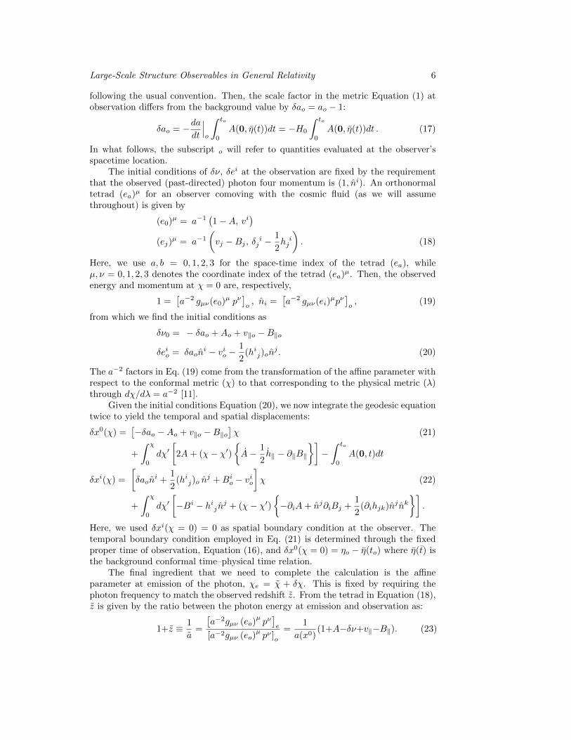
following the usual convention. Then, the scale factor in the metric Equation (1) atobservation differs from the background value by δao = ao − 1:

δao = −dadt

∣∣∣o

∫ to

0

A(0, η(t))dt = −H0

∫ to

0

A(0, η(t))dt . (17)

In what follows, the subscript o will refer to quantities evaluated at the observer’sspacetime location.

The initial conditions of δν, δei at the observation are fixed by the requirementthat the observed (past-directed) photon four momentum is (1, ni). An orthonormaltetrad (ea)µ for an observer comoving with the cosmic fluid (as we will assumethroughout) is given by

(e0)µ = a−1(1−A, vi

)(ej)

µ = a−1(vj −Bj , δ ij −

1

2h ij

). (18)

Here, we use a, b = 0, 1, 2, 3 for the space-time index of the tetrad (ea), whileµ, ν = 0, 1, 2, 3 denotes the coordinate index of the tetrad (ea)µ. Then, the observedenergy and momentum at χ = 0 are, respectively,

1 =[a−2 gµν(e0)µ pν

]o, ni =

[a−2 gµν(ei)

µpν]o, (19)

from which we find the initial conditions as

δν0 = − δao +Ao + v‖o −B‖o

δeio = δaoni − vio −

1

2(hij)on

j . (20)

The a−2 factors in Eq. (19) come from the transformation of the affine parameter withrespect to the conformal metric (χ) to that corresponding to the physical metric (λ)through dχ/dλ = a−2 [11].

Given the initial conditions Equation (20), we now integrate the geodesic equationtwice to yield the temporal and spatial displacements:

δx0(χ) =[−δao −Ao + v‖o −B‖o

]χ (21)

+

∫ χ

0

dχ′[2A+ (χ− χ′)

A− 1

2h‖ − ∂‖B‖

]−∫ to

0

A(0, t)dt

δxi(χ) =

[δaon

i +1

2(hij)o n

j +Bio − vio]χ (22)

+

∫ χ

0

dχ′[−Bi − hij nj + (χ− χ′)

−∂iA+ nj∂iBj +

1

2(∂ihjk)nj nk

].

Here, we used δxi(χ = 0) = 0 as spatial boundary condition at the observer. Thetemporal boundary condition employed in Eq. (21) is determined through the fixedproper time of observation, Equation (16), and δx0(χ = 0) = ηo − η(to) where η(t) isthe background conformal time–physical time relation.

The final ingredient that we need to complete the calculation is the affineparameter at emission of the photon, χe = χ + δχ. This is fixed by requiring thephoton frequency to match the observed redshift z. From the tetrad in Equation (18),z is given by the ratio between the photon energy at emission and observation as:

1+z ≡ 1

a=

[a−2gµν (eo)

µpν]e

[a−2gµν (eo)µpν ]o

=1

a(x0)(1+A−δν+v‖−B‖). (23)


Here, all quantities on the right hand side are evaluated at emission. We find itconvenient to define the perturbation to the logarithm of the scale factor at emission∆ ln a ≡ a(x0)/a− 1. Equation (23) yields

∆ ln a = Ao −A+ v‖ − v‖o +

∫ χ

0

dχ

[−A+

1

2h‖ + B‖

]−H0

∫ to

0

A(0, η(t))dt . (24)

The redshift matching then requires

∆ ln a =∂ ln a

∂η

∣∣∣∣z

(x0 − x0) =H(z)

1 + z(δx0(χ)− δχ) . (25)

We can then solve for the perturbation to the affine parameter yielding

δχ = δx0(χ)− 1 + z

H(z)∆ ln a. (26)

The actual source position is at linear order

xµ(χe) = xµ(χe) + δxµ(χ) = xµ(χ) + [xµ(χe)− xµ(χ)] + δxµ(χ). (27)

To linear order, this gives

∆x0 ≡ x0 − x0 = δx0(χ)− δχ∆xi ≡ xi − xi = δxi(χ) + niδχ. (28)

Finally, we assemble the deflection along the line of sight direction as

∆x‖ = ni∆xi = δx‖ + δx0 − 1 + z

H(z)∆ ln a

= −∫ to

0

A(0, t)dt+

∫ χ

0

dχ

[A−B‖ −

1

2h‖

]− 1 + z

H(z)∆ ln a . (29)

The transverse displacement ∆xi⊥ = Pij∆xj is given by

∆xi⊥ =

[1

2Pij(hjk)o n

k +Bi⊥o − vi⊥o]χ−

∫ χ

0

dχ

[χ

χ

(Bi⊥ + Pijhjknk

)+ (χ− χ)∂i⊥

(A−B‖ −

1

2h‖

)]. (30)

3. Cosmic clock

Perhaps the simplest general relativistic observables are cosmic clocks [16], or standardclocks, a set of events whose proper time (local age of the universe) is accurately known.These cosmic clock events define an observable T (n) as the difference in logarithmof scale factor (ln a) between a constant-proper-time hypersurface tF = const and aconstant-observed-redshift surface z = const. Although phrased as a perturbation inln a, we will frequently refer to T loosely as the proper time perturbation. This isbecause at leading order, the perturbation to the proper time ∆tF (n) at observedredshift z is simply related to T through

∆tF (n) = H−1(z)T (n) . (31)

Since T is defined through two observationally well-defined quantities (proper timeand observed redshift), it is an observable, and the expression for T is gauge-invariant.


The proper time interval dtF along the geodesic of a comoving observer is atlinear order given by

dtF =√−gµνdxµdxν = (1 +A)adη . (32)

Integrating Equation (32), we obtain an expression for tF |x, the proper time of acomoving source passing through x at coordinate time x0, at linear order

tF |x =

∫ x0

0

[1 +A(x, η′)] a(η′)dη′ . (33)

In the case at hand, x0 is the coordinate time at emission, which is different from thecoordinate time η(tF |x) in an unperturbed universe at the proper time tF . The ratioof scale factors at coordinate time x0 and η(tF |x) is

a [η(tF |x)]

a(x0)= 1 +H(x0)

∫ x0

0

A(x, η′)a(η′)dη′ . (34)

The observable T (x) is defined through

T (x) ≡ ln

(a [η(tF |x)]

a

), (35)

where a = (1 + z)−1 is the apparent scale factor at emission. Since ln[a(x0)/a] isprecisely the perturbation ∆ ln a derived in § 2, we arrive at the following simpleexpression for T :

T = ln

(a(x0)

a

a [η(tF |x)]

a(x0)

)= ∆ ln a+ H

∫ η

0

A[x, η′]a(η′)dη′ , (36)

where H ≡ H(z). The gauge invariance of the observable T is explicitly shown inthe Appendix A of [16]. The numerical result for the power spectrum of T inducedby a standard power spectrum of scale-invariant curvature perturbations in ΛCDM isshown in Fig. 3.

A cosmic clock exists whenever we have an observable from which we can definea constant proper-time hypersurface. There are two such classes of observables: 1)cosmic events defined by a unique time and sufficiently short duration, 2) observableswith known time evolution. Cosmic recombination, which led to the emission ofthe cosmic microwave background (CMB) is an example of the former. Neglectingall perturbations including sound waves, last scattering of the Cosmic MicrowaveBackground (CMB) photons happened at a fixed proper time in the local frame, and,therefore, is a cosmic clock event. On scales larger than the angular size of the soundhorizon at recombination, the temperature perturbations in the CMB are then exactlygiven by Θ(n) = −T (n) (Sachs-Wolfe limit [18, 16]). The exact same equation appliesin describing the perturbations in, for example, the surface of neutrino decoupling,Big-Bang Nucleosynthesis and thermal decoupling of baryons from CMB on super-horizon scales. The second case is exemplified by time varying cosmic rulers, whichwill be discussed in the next section.

4. Cosmic ruler, or generalized weak gravitational lensing

We now move on to the cosmic ruler, with which we mean a known spatial scale inthe comoving frame of the cosmic fluid. This could be the size of a galaxy, or thelength at which the correlation function reaches a certain value (we will discuss these


applications in § 4.6). What we observe is the apparent size of this “ruler”, inferredusing the observed positions and redshifts of the endpoints. By comparing this to theknown spatial scale, we can infer the departure from the average angular diameterdistance-redshift relation and the Hubble parameter-redshift relation. In many cases,the size of the ruler will only be known in a statistical sense (for example, galaxy sizes)and will be calibrated by averaging over the entire area of a given survey. Any scatterin the ruler size from its mean value will simply be noise in the measurement of theruler distortions, as long as this scatter is not correlated with large-scale perturbationsthemselves. The latter, “intrinsic” contributions to the distortion of the ruler scalewill not be considered in this paper, although they can be an important source ofcosmological information on their own [19, 20, 21, 22, 23, 24, 15, 25].

As we shall show below, the ruler distortions can be decomposed into scalar,vector, and tensor components on the observer’s sky. The tranverse “sky-plane”components, one scalar and two tensor components, are nothing other than thestandard lensing observables of magnification and shear, respectively. The remainingdistortions, one scalar and two vector components on the sky, involve the line-of-sightcomponent of the ruler. Typically, these can only be observed through spectroscopicmeasurements, since the line-of-sight separation, inferred from the redshift differencebetween the two endpoints, has to be measured with sufficient accuracy. When appliedto correlation functions, these distortions are part of the well-known redshift-spacedistortion effects. However, we stress that the expressions we derive are entirelyindependent of the nature of the ruler considered, and that spectroscopic LSS surveysare just one (albeit important) application of these new observables.

A standard ruler can be generically modeled by two spacetime events separatedby a fixed spacelike separation r0 on a fixed proper time surface of the cosmic fluid.More precisely, the spatial part of the four-velocity uµ of this fluid is determined by

vi =T i0ρ+ p

. (37)

This ruler definition can also be phrased as that the length of the ruler is defined on asurface of constant proper time of comoving observers. This proper time correspondsto the “local age” of the Universe. We are mostly interested in applications to thelarge-scale structure during matter domination. In this case, the cosmic fluid is simplymatter (dark matter + baryons), and there is no ambiguity in this definition; insynchronous-comoving gauge, Equation (37) yields vi = 0. However, this assumptioncan be relaxed very easily, for example one could assume instead that the observersare comoving with the baryon velocity vb.

Then, what we observe is the apparent size of the ruler. Let n, z and n′, z′ denotethe observed coordinates of the endpoints of the ruler, and x and x′ the apparentspatial positions inferred through Equation (13) (see Fig. 1). In the following, wewill assume that the ruler is small compared to the distance χ of the sources as wellas to the typical scale over which we want to measure the spacetime perturbations;it can then be approximated as an infinitesimal distance. For example, in terms ofweak lensing observables, we assume that the angular size of a galaxy is negligiblecompared to the angular scale at which we measure shear correlations. Correctionsto this approximation involve powers of |x − x′|/χ (wide-angle corrections), and/orhigher derivatives of the metric perturbations multiplied by powers of xµ− x′µ.‖ The

‖ For example, for the sky-plane components the leading order correction of this type corresponds tothe lensing flexion. If desired one could straightforwardly extend the treatment to obtain a covariant


apparent physical length of the cosmic ruler is then given by

r2 = a2δij(xi − x′i)(xj − x′j) , (38)

where a = 1/(1 + z) is the observationally inferred scale factor at emission (Fig. 1).The actual separation of the two endpoints of the ruler, xµ, x′µ, as measured in thecomoving frame, on the other hand should be equal to the fixed scale r0:

[gµν(xα) + uµ(xα)uν(xα)] (xµ − x′µ)(xν − x′ν) = r20 . (39)

The four-velocity of comoving observers, whose spatial components are fixed byEquation (37), is given by Eq. (10). With this, Equation (39) yields

− 2a2viδx0δxi + δx0[∆xi −∆x′i] + δxi[∆x0 −∆x′0]

+gij(x

α)

δxiδxj + δxi[∆xj −∆x′j ] + [∆xi −∆x′i]δxj

= r20, (40)

where ∆xµ = ∆xµ(n, z), ∆x′µ = ∆xµ(n′, z′), and the components of the apparentseparation vector are δxµ = xµ − x′µ. In order to evaluate the spatial metric gij(x

α)at the location of the ruler, we use ∆ ln a = a(x0)/a− 1 to obtain at first order

gij(xα) = a2 [(1 + 2∆ ln a) δij + hij ] . (41)

We now again make use of the “small ruler” approximation, so that

∆xi −∆x′i ' δxα ∂

∂xα∆xi. (42)

Like any vector, we can decompose the spatial part of the apparent separation δxi

into parts parallel and transverse to the line of sight:

δx‖ ≡ niδxi

δxi⊥ ≡ Pijδxj = δxi − niδx‖. (43)

In the correlation function literature, δx‖, |δx⊥| are often referred to as π and σ,respectively. Then,

δxα∂

∂xα= (δx0∂η + δx‖∂‖) + δxi⊥∂⊥ i, (44)

where we have similarly defined ∂‖ = ni∂i, ∂⊥ i = P ji ∂j . Since the observed

coordinates xµ by definition satisfy the light cone condition with respect to theunperturbed FRW metric, we have δx0 = −δx‖ in the small-angle approximation.Thus,

δx0∂η + δx‖∂‖ = δx‖(∂‖ − ∂η) = δx‖∂

∂χ= δx‖H(z)

∂

∂z, (45)

where ∂/∂χ is the derivative with respect to the affine parameter at emission. Wethus have

δxα∂

∂xα= δx‖∂χ + δxi⊥∂⊥ i. (46)

Working to first order in perturbations, we then obtain

r20 − r2 = 2∆ ln a r2 + a2hijδxiδxj + 2a2

(v‖δx

2‖ + v⊥ iδx

i⊥δx‖

)+ 2a2δijδx

i(δx‖∂χ + δxk⊥∂⊥ k

)∆xj . (47)

All terms are straightforward to interpret: there are the perturbations to the metricat the ruler location (both from the metric perturbation hij and the perturbation tothe scale factor at emission); the contribution ∝ v from the projection from fixed-ηto fixed-proper-time hypersurfaces; and the difference in the spatial displacements ofthe endpoints of the ruler.

expression for the flexion.


4.1. Clocks and evolving rulers

In the previous section, we have implicitly assumed, as is usually done, that the rulerscale is constant in time, i.e. a non-evolving ruler. However, in many instances incosmology, rulers do evolve over time; that is, the ruler scale r0 depends on the localage of the Universe (proper time of the comoving observer). For example, the meansize of galaxies evolves, and so does the correlation length of large-scale structuretracers. Thus, cosmic rulers in general are also cosmic clocks (§ 3).

Let us consider a standard ruler whose length evolves in time. Then, by usingEquation (34), we can parametrize the time evolution of the proper size of the standardruler r0(a) through its value in an unperturbed Universe as function of the scale factora. The actual proper size of the ruler r0(a(tF |x)), which is the size of the ruler in theconstant-proper-time slicing, relative to the size it evaluates to when inserting theapparent scale factor of emission a = (1 + z)−1, in the constant-observed-redshiftslicing, is given by

r0(a (tF |x))

r0(a)= 1 +

d ln r0(a)

d ln aT (x) , (48)

where T is defined in Eq. (36). Note that we are assuming that ao = 1 at observation,Equation (17), so that r0(1) corresponds to the ruler scale today as calibrated by theobserver. This clearly requires that T = 0 for a locally measured ruler, which is thecase for Eq. (36). To reach this consistency, it is essential that the epoch of observationto is fixed in terms of proper time, rather than coordinate time, as discussed in § 2.

We thus have an additional contribution to the ruler distortion Equation (47)which is proportional to the time derivative of the ruler, explicitly

− 2T d ln r0(a)

d ln ar2 . (49)

4.2. Scalar-vector-tensor decomposition on the sky

It is useful to separate the contributions to Equation (47) in terms of the observedlongitudinal and transverse distortions. For some applications, only the transversedistortions are relevant. This is the case for diffuse backgrounds without redshiftresolution, such as the CMB or the cosmic infrared background, and largely thecase for photometric galaxy surveys. On the other hand, spectroscopic surveys andredshift-resolved backgrounds such as the 21cm emission from high-redshifts are ableto measure the longitudinal displacements as well.

Noting that r2 = a2[δx2‖ + (δx⊥)2], and taking the square root of Equation (47),we obtain the relative perturbation to the physical scale of the ruler as

r − r0r

= C(δx‖)

2

r2c+ Bi

δx‖δxi⊥

r2c+Aij

δxi⊥δxj⊥

r2c, (50)

where we have defined rc ≡ r/a as the apparent comoving size of the ruler. Thequantities multiplying C, Bi, Aij are thus simply geometric factors. The coefficientsare given by

C =d ln r0(a)

d ln aT −∆ ln a− 1

2h‖ − v‖ − ∂χ∆x‖

Bi = − P ji hjkn

k − v⊥i − nk∂⊥ i∆xk − ∂χ∆x⊥i

Aij =d ln r0(a)

d ln aT Pij −∆ ln a Pij −

1

2P ki P l

j hkl


Figure 2. Illustration of the distortion of standard rulers due to the longitudinal(2-)scalar C, (2-)vector B, and transverse components, magnification M and shearγ. The first row shows the projection onto the sky plane, while the second (third)row show the projection onto the line-of-sight and x1⊥ (x2⊥) axes, respectively. Incase of B and γ, we only show one of the two components. From [14]; see alsoFig. 3 in [26].

− 1

2(Pjk∂⊥ i + Pik∂⊥ j) ∆xk, (51)

where ∆x‖, ∆xi⊥ are the parallel and perpendicular components of the displacements∆xi. Note that while we have assumed that the ruler is small, the expressions forC, Bi, Aij are valid on the full sky. Fig. 2 illustrates the distortions induced by thesecomponents. Observationally, we have 6 free parameters (assuming accurate redshiftsare available): the location of one point n, z, and the separation vector described byδxi (with δx0 being fixed by the light cone condition). Using these, we can measurea (2-)scalar on the sphere, C, a 2 × 2 symmetric matrix, Aij , and a 2-componentvector on the sphere, Bi. As a symmetric matrix on the sphere, Aij has a scalarcomponent, given by the trace M ≡ PijAij (magnification), and two componentsof the traceless part which transform as spin-2 fields on the sphere (shear, ±2γ asdefined in Equation (69) below). These quantities are observable and gauge-invariant,although any of the individual contributions in Equation (51) are not. The onlyexception is the proper time perturbation T , which can be isolated by comparing twoco-located rulers which evolve differently in time. Note that we cannot measure anyof the anti-symmetric components, such as the rotation. This is because we havenot assumed the existence of any preferred directions in the Universe. If there is aprimary spin-1 or higher spin field, such as the polarization in case of the CMB, thena rotation can be measured as it mixes the spin±2 components (see, e.g. [27]). In thenext sections we study the three terms C, Bi, Aij in turn.

4.3. Longitudinal scalar

The longitudinal component can be simplified to become

C =d ln r0(a)

d ln aT −∆ ln a

[1−H(z)

∂

∂z

(1 + z

H(z)

)]−A− v‖ +B‖


+1 + z

H(z)

(−∂‖A+ ∂‖v‖ + B‖ − v‖ +

1

2h‖

). (52)

The first line contains the contributions due to the fact that the size of the ruler evolvesin time, the scale factor at emission is perturbed from 1/(1 + z), and the fact thatthe distance-redshift relation evolves, in addition to the perturbation to the metricat the source location (−A) and the projection from coordinate-time to proper-timehypersurfaces (B‖−v‖). The contributions from the line-of-sight derivative of the line-of-sight displacements (∝ (1 + z)/H(z)) are given in the second line. Note the term∂‖v‖, which is the dominant term on small scales in the conformal-Newtonian gauge.This term is also responsible for the linear redshift-space distortions [28]. Apart fromthe perturbation to the scale factor at emission, C does not involve any integral terms;this is expected since C is the only term remaining if the two lines of sight coincide(n = n′). In this case, the two rays share the same path from the closer of the twoemission points, and no quantities integrated along the line of sight can contribute tothe perturbation of the ruler.

Restricting to the synchronous-comoving and conformal-Newtonian gauges,respectively, we obtain

(C)sc = − (∆ ln a)sc

[1− d ln r0(a)

d ln a−H(z)

∂

∂z

(1 + z

H(z)

)]+

1 + z

2H(z)h‖. (53)

(C)cN =d ln r0(a)

d ln aTcN − (∆ ln a)cN

[1−H(z)

∂

∂z

(1 + z

H(z)

)]−Ψ− v‖ +

1 + z

H(z)

(−∂‖Ψ + ∂‖v‖ − v‖ + Φ

). (54)

Note that in case of the sc-gauge expression, the redshift-space distortion term isincluded in the last term, through h‖/2 = D + ∂2‖E. Fig. 3 shows the angular powerspectrum of C due to standard adiabatic scalar perturbations in a ΛCDM cosmology(the details of the calculation are given in Appendix F of [14]). Clearly, C is of the sameorder as the matter density contrast in synchronous-comoving gauge on all scales. Inparticular, the velocity gradient term dominates over all other contributions.

4.4. Vector

Next, we have the two-component vector, which can be written as

Bi = −v⊥i +B⊥i +1 + z

H(z)∂⊥i∆ ln a . (55)

As expected, this vector involves the transverse derivative of the line-of-sightdisplacement and the line-of-sight derivative of the transverse displacement. Notethat these two quantities are not observable individually.

Using the spin±1 unit vectors m±, Bi can be decomposed into spin±1components:

Bi = +1Bmi+ + −1Bmi

−

±1B ≡ mi∓Bi = −v± +B± +

1 + z

H(z)∂±∆ ln a, (56)

where we have used the notation of Equation (9). Similar to before, we can specializethis general result to the synchronous-comoving and conformal-Newtonian gauges:

(±1B)sc =1 + z

2H(z)

∫ χ

0

dχχ

χ∂±h‖ (57)


Figure 3. Angular power spectra of the different standard ruler perturbationsproduced by a standard scale-invariant power spectrum of curvature perturba-tions: C, E-mode of Bi, E-mode of the shear γ, magnification M, and clockperturbation T . C and M are calculated for a non-evolving ruler, and all are for asharp source redshift of z = 2. For comparison, the thin dotted line shows the an-gular power spectrum at z = 2 of the matter density field in synchronous-comovinggauge. Note that all quantities shown here, except for δscm, are gauge-invariantand (in principle) observable. Adapted from [14, 16].

(±1B)cN = −v± +1 + z

H(z)∂±∆ ln a

= −v± +1 + z

H(z)

(− ∂±Ψ + ∂±[v‖ − v‖o] +

∫ χ

0

dχχ

χ∂±(Φ− Ψ)

). (58)

On small scales, the dominant contribution to Bi comes from the transverse derivativeof the line-of-sight component of the velocity ∂±v‖, which is of the same order as thetidal field.

Applying the spin-lowering operator ð to 1B yields a spin-zero quantity (seeAppendix A of [14]), which can be expanded in terms of the usual spherical harmonics.We then obtain the multipole coefficients of B as

aBlm(z) = −

√(l − 1)!

(l + 1)!

∫dΩ

[ð 1B(n, z)

]Y ∗lm(n). (59)

An equivalent result is obtained for ð−1B. In general, the multipole coefficients aBlmare complex, so that we can decompose them into real and imaginary parts,

aBlm = aBElm + i aBBlm . (60)

One can easily show (Appendix A of [14]) that under a change of parity aBElm transformas the spherical harmonic coefficients of a vector (parity-odd), whereas aBBlm , pickingup an additional minus sign, transform as those of a pseudo-vector (parity-even).These thus correspond to the polar (“E”) and axial (“B”) parts of the vector Bi.As required by parity, scalar perturbations do not contribute to the axial part aBBlm .Thus, a measurement of the vector component Bi of standard ruler distortions offersan additional possibility to probe gravitational waves with large-scale structure, as


tensor modes do contribute to aBBlm . Thus, in principle the axial component of Bicould be of similar interest for constraining tensor modes as weak lensing B-modes[15].

The power spectrum of the E-mode of B due to standard scalar perturbationsis shown in Figure 3. The dominant contribution to Bi for a given Fourier mode ofthe matter density contrast in synchronous-comoving gauge is ∝ k⊥k‖/k

2 δscm(k, z),while the corresponding contribution to the longitudinal scalar C is ∝ k2‖/k

2 δscm(k, z).

Even though approximate scaling arguments suggest that CC(l), CEEB (l) should scale

roughly equally with l, the different structure in terms of k‖, k⊥ (together with theshape of the matter power spectrum in ΛCDM) leads to a faster scaling of CB(l) withl for l . 500 (see discussion in [14]).

4.5. Transverse tensor: shear and magnification

Finally, we have the purely transverse component,

Aij =d ln r0(a)

d ln aT Pij −∆ ln a Pij −

1

2P ki P l

j hkl − ∂⊥ (i∆x⊥ j) −1

χ∆x‖Pij , (61)

where we have again inserted projection operators for clarity (note that Pij serves asthe identity matrix on the sphere). As a symmetric matrix on the sphere, Aij hasa scalar component, given by the trace A, and two components of the traceless partwhich transform as spin-2 fields on the sphere. The trace corresponds to the changein area on the sky subtended by two perpendicular standard rulers. Thus, it is equalto the magnification M (see also Fig. 2). The two components of the traceless partcorrespond to the shear γ. If we choose a fixed coordinate system (eθ, eφ, n), we canthus write

Aij =

(M/2 + γ1 γ2

γ2 M/2− γ1

). (62)

Below, we will derive the magnification and shear for the general perturbed FRWmetric Equation (1).

4.5.1. Magnification Taking the trace of Equation (61) yields

M≡ PijAij = 2d ln r0(a)

d ln aT − 2∆ ln a− 1

2

(h− h‖

)− 2

χ∆x‖ + 2κ . (63)

The magnification is directly related to the fractional perturbation in the angulardiameter and luminosity distances (see [29, 30]) through

∆DL

DL=

∆DA

DA= −1

2M, (64)

where the first equality for the luminosity distance follows from the conservation ofthe photon phase space density. That is, M describes both the change in apparentangular size of a spatial ruler as well as the change in observed flux of a standardcandle. The contributions to the magnification are straightforwardly interpreted ascoming from the time evolution of ruler scale (or intrinsic source luminosity, if appliedto standard candles) through the proper time perturbation T ; from the conversion ofcoordinate distance to physical scale at the source (both from the perturbation to thescale factor ∆ ln a and the metric at the source projected perpendicular to the line of


sight, h − h‖); from the fact that the entire ruler is moved closer or further away by∆x‖; and finally from the coordinate convergence κ defined through

κ = −1

2∂⊥ i∆x

i⊥. (65)

This term is the dominant contribution toM on small scales. However, the coordinateconvergence is a gauge-dependent quantity; see for example Appendix B2 in [11]. Inconformal-Newtonian gauge, it assumes its familiar form,

(κ)cN = − v‖o +1

2

∫ χ

0

dχχ

χ(χ− χ)∇2

⊥ (Ψ− Φ) , (66)

with an additional term −v‖o contributing to the dipole of κ only, which correspondsto the relativistic aberration effect at linear order. An explicit expression for themagnification in general gauge is straightforward to obtain, however it becomeslengthy. Here we just give the results for the two most popular gauge choices. First,in synchronous-comoving gauge [Equation (2)] we obtain

(M)sc = 2

[d ln r0(a)

d ln a− 1

](∆ ln a)sc−

1

2(h−h‖)+2(κ)sc−

2

χ∆x‖ , (67)

where

(κ)sc = −1

4

[ho − 3(h‖)o

]+

1

2

∫ χ

0

dχ

[(∂l⊥hlk)nk +

1

χ

(h− 3h‖

)− 1

2(χ− χ)

χ

χ∇2⊥h‖

].

In conformal-Newtonian gauge [Equation (3)], we have (h − h‖)/2 = 2Φ, so that themagnification in this gauge becomes

(M)cN = 2d ln r0(a)

d ln aTcN +

[−2 +

2

aHχ

](∆ ln a)cN − 2Φ + 2(κ)cN

− 2

χ

∫ χ

0

dχ (Ψ− Φ) +2

χ

∫ to

0

dtΨ(0, t) . (68)

The last term in Equation (68) is a pure monopole and thus usually absorbed in theruler calibration (since r0 can rarely be predicted from first principles without anydependence on the background cosmology). Nevertheless, the monopole of M is inprinciple observable, and including this term ensures that gauge modes (for examplesuperhorizon metric perturbations) do not affect its value.

We have thus arrived at a general gauge-invariant expression for the magnificationwithout having to perform lengthy calculations. Moreover, the physical startingpoint from a standard ruler scale has allowed us to identify a previously overlookedcontribution to the magnification. This contribution is given by the clock variableT and becomes relevant whenever the ruler scale evolves over cosmic time. In manyapplications, this is the case, although T is sub-dominant to the lensing convergenceκ on all but the largest scales [16].

4.5.2. Shear We now consider the traceless part of Aij , given by

γij(n) ≡ Aij −1

2PijM

= −1

2

(P ki P l

j −1

2PijPkl

)hkl − ∂⊥(i∆x⊥ j) − Pij κ. (69)


Here, the terms ∝ Pij in Equation (61) drop out. The last two terms here are whatcommonly is regarded as the shear, i.e. the trace-free part of the transverse derivativesof the transverse displacements. The first term on the other hand is important toconstruct an observable as it ensures a gauge-invariant result. This is the term referredto as “metric shear” in [13]. Its physical significance becomes clear when constructingthe Fermi normal coordinates, or local inertial frame, for the region containing thestandard ruler.

Consider a region of spatial extent R, say centered on a given galaxy, and enclosingour standard ruler. We can construct orthonormal Fermi normal coordinates [31, 32]around the center of this region, which follows a timelike geodesic, by choosing theorigin to be located at the center of the region at all times, and the time coordinateto be the proper time along the geodesic. As a local inertial frame, the spacetime inthe Fermi coordinates (tF , x

iF ) is Minkowski close to the geodesic, with corrections

proportional to x2F /R

2c where Rc is the curvature scale of the spacetime. Thus, as

long as these corrections to the metric are negligible, there is no preferred direction inthis frame, and the size r0 of the standard ruler has to be (statistically) independentof the orientation. The most obvious example is galaxy shapes, which are used forcosmic shear measurements. In the Fermi frame, when neglecting tidal alignments,galaxy orientations are statistically random. As shown in [14, 15], the transformationfrom global coordinates to Fermi coordinates for a purely spatial metric perturbationhij is given by

a−1xiF = xi +1

2hij(0)xj +O(∂mhklx

2). (70)

In order to obtain the shear relative to the Fermi frame, we need to add thetransformation Equation (70) to the displacements ∆xi:

∆xi → ∆xi +1

2hij(0)xj . (71)

With these new displacements, the transverse derivative of the transverse displacementbecomes

∂⊥(i∆x⊥ j) → ∂⊥(i∆x⊥ j) +1

2P ki P k

j hkl +O(∂khij [x− x′]) , (72)

where the last term is negligible in the small-ruler approximation. This agreesexactly with the result derived above, Equation (69) [after subtracting the trace ofEquation (72)]. Note that the Fermi coordinates are uniquely determined up to threeEuler angles. The statement that galaxy orientations are random in this frame is thuscoordinate-invariant.

γij is a symmetric trace-free tensor on the sphere, and can thus be decomposedinto spin±2 components (in analogy to the polarization of the CMB). FollowingAppendix A in [14] (see also [33]) we can write γij as

γij = 2γ mi+m

j+ + −2γ m

i−m

j−

±2γ = mi∓m

j∓γij , (73)

where ±2γ are spin±2 functions on the sphere (in analogy to the combination of Stokesparameters Q ± iU). The general, lengthy expression for the shear components canbe found in [14]. Here we give the expressions for the synchronous-comoving (sc) andthe conformal-Newtonian (cN) gauges (note that h± = 0 in cN gauge):

(±2γ)sc = − 1

2h± −

1

2(h±)o −

∫ χ

0

dχ

[(1− 2

χ

χ

)(∂±hkl)m

k∓n

l − 1

χh± (74)


+ (χ− χ)χ

χ

1

2(mi∓m

j∓∂i∂jhlk)nlnk

]

(±2γ)cN =

∫ χ

0

dχ (χ− χ)χ

χmi∓m

j∓∂i∂j (Ψ− Φ) . (75)

We see that Equation (75) recovers the “standard” result; in other words, thereare no additional relativistic corrections to the shear in cN gauge. This is notsurprising following our arguments above: in the conformal-Newtonian gauge, thetransformation Equation (70) from global coordinates to the local Fermi frame isisotropic since hij = 2Φδij . Thus, it does not contribute to the shear. Note howeverthat this only applies to scalar perturbations; when considering vector or tensorperturbations, Equation (74) is the relevant expression which does contain termsbeyond the derivative of the deflection angle. This is also of relevance to studiesof gravitational lensing of the CMB by gravitational waves [34] (see also [15]).

Fig. 3 shows the angular power spectrum of shear and magnification due to scalarperturbations for a sharp source redshift z = 2. For l & 10, the results follow thefamiliar relation CM(l) = 4CEEγ (l), valid when all relativistic corrections to themagnification become irrelevant so that M ' 2κ. These corrections slightly increasethe magnification for small l. We also see that γ and M are suppressed with respectto C and B (on smaller scales), at least when the latter are evaluated for a sharp sourceredshift. This is a well-known consequence of the projection with the broad lensingkernel, leading to a cancellation of modes that are not purely transverse (see e.g. [35]).

4.6. Applications

Consider a galaxy whose image projected on the sky, as seen by a local observer,has an “intrinsic” intensity or surface brightness I(θ) (here θ = 0 corresponds to thecentroid of the galaxy). Then, the ruler formalism immediately yields the observedintensity through

Iobs(θi) = I

(θi −Aij θj

)=

[1−A j

i θi ∂

∂θj

]I(θ) +O([Aij ]2) , (76)

where Aij is the sky-plane projection of the ruler perturbations, Equation (51), andwe have expanded to linear order. This is the well known effect of weak gravitationallensing on an image.

Now consider the case of a spectroscopic survey, where we measure the small-scalecorrelation function ξ(r, z) as a function of the three-dimensional separation vector rand the redshift z. As shown in [36], the observed correlation function is given interms of the expectation value of the intrinsic correlation function ξ(r, z) by

ξ(r, τ) =[1− aij(x)ri∂jr + T (x)∂z + 2〈δ〉(x)

]ξ(r; z) , (77)

where 〈δ〉 is the mean observed overdensity of the tracer within the volume over whichξ is measured (see the next section), which simply serves to rescale the local meandensity. The tensor aij contains the ruler perturbations:

aij = C ninj + n(iPj)k Bk + PikPjlAkl , (78)

where we have inserted trivial projection operators for B, A.These examples serve to illustrate how the standard ruler formalism can be

immediately applied to predict cosmological observables.


5. Galaxy clustering

The statistics (correlation functions) of large-scale structure tracers have a long historyas one of the most important observational tools in cosmology. The fundamentalbuilding block of these statistics is the observed number density ng of tracers inferredfrom their apparent positions on the sky and redshifts. In this section, we showhow ng is related to the spacetime perturbations in the relativistic context. For this,we need to consider two effects: first, the effect of spacetime perturbations on thepropagation of light emitted from the sources systematically distorts the observedgalaxy density contrast [7, 8, 9, 10, 37, 11, 12]. Second, we need to relate the numberdensity of galaxies to the matter density, a procedure commonly knows as biasing,which involves additional subtleties in the relativistic context [37, 11].

As discussed earlier in § 2.2, observers chart galaxies according to the observedposition xµ = (η0 − χ, nχ). The galaxy density is estimated based on the observedspatial coordinate x = χn, and then compared with the mean number density ng(z) at

fixed observed coordinate to infer the local galaxy overdensity δg. Once corrected forwindow function and selection effects, the mean galaxy number density only dependson the observed redshift. In this sense, the observed density contrast δg can be seenas defined in a constant-observed-redshift gauge. Throughout, we will assume thatng(z) corresponds to the true mean density of galaxies, i.e. we will neglect the effectof super-survey modes.

The number of galaxies enclosed in a spatial volume V defined in the observedcoordinates is given by

N(V ) =

∫V

d3x√−g(x)ng(x)εµνρσu

µ(x)∂xν

∂x1∂xρ

∂x2∂xσ

∂x3, (79)

where we have transformed the integral to observed coordinates x, V is a spatialvolume on a constant-observed-redshift slice, and x(x) denotes the true spacetimelocation corresponding to the observed location x. ng is the physical (as opposed tocomoving) number density of tracers in the perturbed FRW coordinates [Eq. (1)].

We now employ a useful trick. Rather than expressiong ng in terms of the galaxydensity perturbation δg in some arbitrary gauge, we fix the coordinates to the constant-observed-redshift (“or”) gauge. We thus write ng in term of the mean number densityng and the perturbation δorg to the comoving number density in the constant-observed-redshift gauge as

a3ng(x) = a3ng(z)[1 + δorg (x, z)

], (80)

where z is the observed redshift corresponding to the spacetime location x, anda = 1/(1 + z). Since δorg is already first order, we can neglect the distinction betweenx(x) and x in its argument. Eq. (80) can be understood as the definition of δorg .

We rewrite the right hand side of Eq. (79) in terms of the metric perturbation tolinear order as

N(V ) =

∫V

d3x

(1 +A+

h

2

)a3ng(z)

[1 + δorg (x, z)

]((1−A)

∣∣∣∣ ∂xi∂xj

∣∣∣∣+ v‖

). (81)

The observed galaxy number density ng, on the other hand, satisfies by definition

N =

∫d3x a3ng(x, z) . (82)


By equating the two, we find the observed galaxy density contrast as

δg(x) ≡ ng(x, z)

ng(z)− 1 = δorg (x, z) +

h

2+ ∂‖∆x‖ +

2∆x‖

χ− 2κ+ v‖ . (83)

Here, we have used the Jacobian∣∣∣∣ ∂xi∂xj

∣∣∣∣ = 1 +∂∆xi

∂xi= 1 + ∂‖∆x‖ +

2∆x‖

χ− 2κ (84)

with the lensing convergence κ defined in Equation (65). All contributions in Eq. (83)apart from δorg thus correspond to the apparent modulation of the galaxy abundancedue to volume distortion effects.

Next, we have to relate δorg in Equation (83) to the matter density through abiasing relation. The galaxy density contrast δorg in Equation (83) is defined in theconstant-observed-redshift slicing, while the linear bias relation between galaxy densitycontrast and matter density contrast holds only on constant-proper-time (“pt”) slices.This is because in the large-scale limit, galaxies only know about the local age ofthe Universe and the local matter density (see [37] and §III in [11] for a detaileddiscussion).P The shift between the constant-observed-redshift slice and constant-proper-time slice is given by the observable T that we have discussed in § 3. Then,the relation between δorg (x, z) and the matter perturbation δptm in the constant-proper-time (or synchronous) gauge is given by the standard linear gauge transformation

δorg (x, z) = b δptm +d(a3ng)

d ln aT ≡ b δptm + beT , (85)

where we have introduced the dimensionless parameter be quantifying the evolutionof the mean comoving number density of tracers. Note that this relation only involvesobservable quantities, so that both b and be are well defined and gauge-invariant. Italso serves as the unambiguous starting point for extending the bias relation to higherorder in perturbations, for example by adding a term b2/2 (δptm )2 to the right handside.

Finally, δptm is related to the matter density perturbation δm in the chosen gaugethrough

δptm = δm + 3H

∫ η

0

A(x, η)a(η)dη . (86)

Combining the last two equations, we find the galaxy density contrast on the constant-observed-redshift slice in terms of the density contrast in an arbitrary gauge as

δorg (x, z) = b

[δm + 3H

∫ η

0

A(x, η)a(η)dη

]+ beT . (87)

This yields our final expression:

δg(x, z) = b

[δm + 3H

∫ η

0

A(x, η)a(η)dη

]+ be T +

1

2h+∂χ∆x‖+

2∆x‖

χ−2κ+v‖ .(88)

P This assumes that there are no additional degrees of freedom relevant on large scales, such as darkenergy perturbations, neutrinos, or fifth forces. The impact of these on the general linear biasingrelation is an interesting question, though beyond the scope of this review.


Here,

∂χ∆x‖ = A−B‖ −1

2h‖ −H(z)

∂

∂z

(1 + z

H(z)

)∆ ln a

− 1 + z

H(z)

(−∂‖A+ ∂‖v‖ − v‖ +

1

2h‖ + B‖

). (89)

One subtlety we have neglected so far is that observational selection effects canmodify the observed galaxy density, Equation (88). Usually surveys observe galaxiesabove a certain magnitude threshold. Weak lensing magnifies/de-magnifies the flux ofthe source galaxies and therefore induces another contribution to the observed galaxydensity (magnification bias). For a population of galaxies at fixed redshift z withcumulative luminosity function n(> Lmin), we define

Q ≡ −d ln n(> Lmin)

d lnLmin, (90)

whereM is the magnification discussed in detail in § 4.5.1. Then, the contribution toδg induced by the lensing magnification [Equation (63)] is QM. Note that our “ruler”here is the luminosity of galaxies at the cutoff Lmin, so that d ln r0/d ln a in Eq. (63) isto be replaced with the evolution of the intrinsic luminosity of galaxies with L = Lmin

at z, d lnLmin/d ln a, in order to take the evolving ruler effect into account (§ 4.1). Wefinally obtain the observed density contrast including magnification bias as

δg(x, z) = b

[δm + 3H

∫ η

0

A(x, η)a(η)dη

]+

(be + 2Q

[d lnLmin

d ln a− 1

])T

+ 2QH∫ η

0

A(x, η)a(η)dη +1

2(1−Q)h+

Q2h‖ + ∂χ∆x‖ + (1−Q)

2

χ∆x‖

− 2(1−Q)κ+ v‖ . (91)

Eq. (91) provides the complete result for the observed overdensity of a tracer atlinear order in a general gauge; to our knowledge, this is the first time an expression forδg has been given in a general gauge with a physical treatment of galaxy bias. Whenrestricted to conformal-Newtonian gauge, this agrees with [10, 37] (note the discussionaround Eq. (31) of the former reference); restricting to synchronous-comoving gaugeyields the results derived in [11]. Note also that all previous references implicitlyassumed that d lnLmin/d ln a, which induces an apparent density contrast due to timeevolution of the luminosity function, is zero (though since this term is proportional toT , it is expected to be subdominant on all scales, see Fig. 3). Throughout, we haveassumed a sharp source redshift. The projection over a wider photometric redshift binis straightforward.

Assuming the coefficients b, be, Q are all of order unity, the various terms inEq. (91) can be ranked in terms of relative importance according to their scaling inFourier space. The largest terms, “order 1”, are

δO(1)g = b δm +

1 + z

H∂‖v‖ − 2(1−Q)κ . (92)

Here, we have assumed that one of the standard gauges is chosen where δm ' δptm onsmall scales (this includes conformal-Newtonian gauge). Equation (92) is the standardsmall-scale result for the apparent galaxy overdensity, including the leading redshift-space distortion (“Kaiser formula” [28]) and magnification bias. Next, there arecontributions suppressed by aH/k (“velocity-type”) and (aH/k)2 (“potential-type”).


The potential-type contributions have the same k-dependence as the scale-dependentbias from primordial non-Gaussianity of the local type [38]. These are numerically thesmallest contributions, and amount to the effect of local primordial non-Gaussianitywith fNL . 1, as shown in [11]. The velocity-type contributions, which are ∝ v‖ and∂‖Ψ in case of conformal-Newtonian gauge, are larger and likely to be measurable inupcoming surveys [39].

6. Conclusion and future work

In this paper, we have derived the effects of light deflection in the perturbed FRWuniverse, and an associated set of observables in the large-scale structure of theUniverse. Light deflection distorts the observed position and redshift of cosmic events,and such distortions can be measured for events with known cosmic age (cosmic clock)or length scale (cosmic ruler). Distortions in the cosmic clocks are described bythe observable T , which is the redshift perturbation between the constant-proper-time slicing and the constant-observed-redshift slicing (an example being the CMBtemperature perturbations in the Sachs-Wolfe limit); distortions in the cosmic rulersare completely described by six observables which are classified as two scalars (Cand the magnification M), two components of a divergence-free vector (Bi), and twocomponents of a tensor (shear γij) on the celestial sphere.

We have also presented the fully general expression for the observed galaxy densitycontrast at linear order, a fundamental galaxy clustering observable, including thevolume distortion due to the light deflection, evolving number density, galaxy densitybias, as well as the magnification bias generalized to evolving luminosity function.

All expressions in this paper are derived at linear order in density, velocity, andmetric perturbations, but in their most general form, sometimes referred to as gaugeready form. Therefore, all expressions in this paper can be trivially restricted toany specific gauge. We show gauge-fixed examples for the conformal Newtonian (cN)gauge and synchronous comoving (sc) gauge in § 4. Extending the calculations tohigher order should also be straightforward, albeit tedious, by following the logicalsteps described in this paper. In fact, three pre-prints ([40, 41, 42]) extending thecalculation of the observed galaxy density contrast to second order have appeared bythe time this paper was written.

In summary, we now have a general relativistic description for the complete setof large-scale observables of the large-scale structure (T , C, Bi, M, γij as well as δg).Hence, future work can focus on the applications of these results. In particular, inconjunction with future large-scale structure surveys mapping a significant fractionof the observable universe (V & 100 [Gpc/h]3) such as Euclid, LSST and SKA, weenvisage three directions that this line of research should pursue:

First of all, all expressions shown in this paper, with the exception of the biasingrelation, Eq. (85), only depend on kinematics of light propagation, and, therefore,hold for any metric theory of gravity. Non-smooth Dark Energy as well as modifiedgravity theories predict different relations between the aforementioned observables andthe cosmic density perturbations than the standard ΛCDM or smooth Dark Energyscenarios. This effect has only recently been explored for galaxy clustering [43], and itwould be interesting to see how large the impact could be in other large-scale structureobservables.

The relativistic effects discussed here appear on near horizon scales k ∼0.001 h/Mpc. Our expressions for T , C, B,M, γ, δg are valid on the full sky and


can immediately be used to calculate angular auto- and cross-correlations C(`) onarbitrarily large scales. However, for spectroscopic surveys, angular correlations inmany narrow redshift bins might not be the optimal approach. While on sufficientlysmall scales the flat-sky approximation can be used, on large scales conventionalFourier-basis decompositions must be modified to include the effects from skycurvature as well as time evolution of the cosmic structure [44, 45, 46].

Finally, going beyond the power spectrum, it is interesting to investigate theimpact of relativistic effects on higher order correlation functions. In general, thisrequires the calculation of the relativistic observables to higher order, e.g. secondorder for the bispectrum of cosmic shear and galaxy clustering. However, most of thesignal-to-noise in the bispectrum on very large scales is in the squeezed limit, whereone large-scale mode is correlated with two small-scale modes. In this limit, one canuse a trick to circumvent the second order calculation [36]. The bispectrum in thislimit is then entirely determined by the linear order ruler distortions of the small-scalecorrelation function that are described in § 4.6 (along with any primordial contributiondue to local-type primordial non-Gaussianity).

In summary, the relativistic effects that we discuss here must be includedwhenever very large scale modes are measured, and are thus crucial in order to fullyexploit the information in future large-scale structure surveys. Fortunately, they canbe accurately predicted in terms of only a few tracer-dependent free parameters.

References

[1] Bennett C L, Larson D, Weiland J L, Jarosik N, Hinshaw G, Odegard N, Smith K M, Hill R S,Gold B, Halpern M, Komatsu E, Nolta M R, Page L, Spergel D N, Wollack E, Dunkley J,Kogut A, Limon M, Meyer S S, Tucker G S and Wright E L 2013 Astrophys. J. Supp. 20820 (Preprint 1212.5225)

[2] Komatsu E, Bennett C L, Barnes C, Bean R, Bennett C L, Dore O, Dunkley J, Gold B, GreasonM R, Halpern M, Hill R S, Hinshaw G, Jarosik N, Kogut A, Komatsu E, Larson D, LimonM, Meyer S S, Nolta M R, Odegard N, Page L, Peiris H V, Smith K M, Spergel D N, TuckerG S, Verde L, Weiland J L, Wollack E and Wright E L 2014 Progress of Theoretical andExperimental Physics 2014 06B102 (Preprint 1404.5415)

[3] Ade P A R et al. 2013 arXiv:1303.5062 (Preprint 1303.5062)[4] Planck Collaboration, Ade P A R, Aghanim N, Armitage-Caplan C, Arnaud M, Ashdown M,

Atrio-Barandela F, Aumont J, Baccigalupi C, Banday A J and et al 2013 ArXiv e-prints(Preprint 1303.5076)

[5] Cole S et al. (2dFGRS) 2005 MNRAS 362 505–534 (Preprint astro-ph/0501174)[6] Eisenstein D J et al. (SDSS) 2005 Astrophys. J. 633 560–574 (Preprint astro-ph/0501171)[7] Yoo J, Fitzpatrick A L and Zaldarriaga M 2009 PRD 80 083514–+ (Preprint 0907.0707)[8] Yoo J 2010 PRD 82 083508–+ (Preprint 1009.3021)[9] Bonvin C and Durrer R 2011 ArXiv e-prints (Preprint 1105.5280)

[10] Challinor A and Lewis A 2011 ArXiv e-prints (Preprint 1105.5292)[11] Jeong D, Schmidt F and Hirata C M 2012 PRD 85 023504 (Preprint 1107.5427)[12] Jeong D and Schmidt F 2012 PRD 86 083512 (Preprint 1205.1512)[13] Dodelson S, Rozo E and Stebbins A 2003 Physical Review Letters 91 021301–+ (Preprint

arXiv:astro-ph/0301177)[14] Schmidt F and Jeong D 2012 PRD 86 083527 (Preprint 1204.3625)[15] Schmidt F and Jeong D 2012 PRD 86 083513 (Preprint 1205.1514)[16] Jeong D and Schmidt F 2013 ArXiv e-prints (Preprint 1305.1299)[17] Pyne T and Birkinshaw M 1993 Astrophys. J. 415 459 (Preprint arXiv:astro-ph/9303020)[18] Sachs R K and Wolfe A M 1967 Astrophys. J. 147 73–+[19] Catelan P, Kamionkowski M and Blandford R D 2001 MNRAS 320 L7–L13 (Preprint arXiv:

astro-ph/0005470)[20] Hirata C M and Seljak U 2004 PRD 70 063526 (Preprint arXiv:astro-ph/0406275)[21] Brown M L, Taylor A N, Hambly N C and Dye S 2002 MNRAS 333 501–509 (Preprint

arXiv:astro-ph/0009499)

1212.5225

1404.5415

1303.5062

1303.5076

astro-ph/0501174

astro-ph/0501171

0907.0707

1009.3021

1105.5280

1105.5292

1107.5427

1205.1512

arXiv:astro-ph/0301177

1204.3625

1205.1514

1305.1299







[22] Blazek J, McQuinn M and Seljak U 2011 JCAP 5 10 (Preprint 1101.4017)[23] Joachimi B, Mandelbaum R, Abdalla F B and Bridle S L 2011 Astron. Astrophys. 527 A26

(Preprint 1008.3491)[24] Pen U L, Sheth R, Harnois-Deraps J, Chen X and Li Z 2012 ArXiv e-prints (Preprint 1202.5804)[25] Schmidt F, Pajer E and Zaldarriaga M 2014 PRD 89 083507 (Preprint 1312.5616)[26] Sachs R 1961 Royal Society of London Proceedings Series A 264 309–338[27] Gluscevic V, Kamionkowski M and Cooray A 2009 PRD 80 023510 (Preprint 0905.1687)[28] Kaiser N 1987 MNRAS 227 1–21[29] Hui L and Greene P B 2006 PRD 73 123526 (Preprint arXiv:astro-ph/0512159)[30] Bonvin C, Durrer R and Gasparini M A 2006 PRD 73 023523–+ (Preprint arXiv:astro-ph/

0511183)[31] Fermi E 1922 Atti Acad. Naz. Lincei Rend. Cl. Sci. Fiz. Mat. Nat. 31 21[32] Manasse F K and Misner C W 1963 Journal of Mathematical Physics 4 735–745[33] Hu W 2000 PRD 62 043007 (Preprint arXiv:astro-ph/0001303)[34] Book L G, Kamionkowski M and Souradeep T 2011 ArXiv e-prints (Preprint 1109.2910)[35] Jeong D, Schmidt F and Sefusatti E 2011 PRD 83 123005 (Preprint 1104.0926)[36] Pajer E, Schmidt F and Zaldarriaga M 2013 PRD 88 083502 (Preprint 1305.0824)[37] Baldauf T, Seljak U, Senatore L and Zaldarriaga M 2011 ArXiv e-prints (Preprint 1106.5507)[38] Dalal N, Dore O, Huterer D and Shirokov A 2008 PRD 77 123514–+ (Preprint 0710.4560)[39] Yoo J, Hamaus N, Seljak U and Zaldarriaga M 2012 PRD 86 063514 (Preprint 1206.5809)[40] Yoo J and Zaldarriaga M 2014 ArXiv e-prints (Preprint 1406.4140)[41] Bertacca D, Maartens R and Clarkson C 2014 ArXiv e-prints (Preprint 1405.4403)[42] Di Dio E, Durrer R, Marozzi G and Montanari F 2014 ArXiv e-prints (Preprint 1407.0376)[43] Lombriser L, Yoo J and Koyama K 2013 PRD 87 104019 (Preprint 1301.3132)[44] Yoo J and Desjacques V 2013 PRD 88 023502 (Preprint 1301.4501)[45] Di Dio E, Montanari F, Lesgourgues J and Durrer R 2013 JCAP 11 044 (Preprint 1307.1459)[46] Di Dio E, Montanari F, Durrer R and Lesgourgues J 2014 JCAP 1 042 (Preprint 1308.6186)

1101.4017

1008.3491

1202.5804

1312.5616

0905.1687





1109.2910

1104.0926

1305.0824

1106.5507

0710.4560

1206.5809

1406.4140

1405.4403

1407.0376

1301.3132

1301.4501

1307.1459

1308.6186

Large-Scale Structure Observables in General

Documents

Transcript of Large-Scale Structure Observables in General