Large-Scale Diagnostics of Tropical Cyclogenesis … Diagnostics of Tropical Cyclogenesis Potential...

Large-Scale Diagnostics of Tropical Cyclogenesis Potential Using EnvironmentVariability Metrics and Logistic Regression Models

JEFFREY J. WATERS, JENNI L. EVANS, AND CHRIS E. FOREST

The Pennsylvania State University, University Park, Pennsylvania

(Manuscript received 29 June 2011, in final form 29 February 2012)

ABSTRACT

The authors propose that inclusion of medium- to high-frequency variability information will provide

improved metrics of tropical cyclogenesis (TCG) applicable to climate GCM diagnostics. Capabilities of

the Community Atmosphere Model version 3.1 (CAM3.1) GCM are assessed for detecting both large-scale

and localized conditions for TCG in the tropical North Atlantic by comparison with the 40-yr European

Centre for Medium-Range Weather Forecasts Re-Analysis (ERA-40) and observed TCG occurrences.

CAM3.1 seasonality of large-scale environmental factors conducive to TCG compares favorably with the

ERA-40. It is determined that most of the TCG-related high-frequency temporal variability in the ERA-40

is explained by dynamic variability; each of the CAM3.1 ensemble members has lower variability in these

dynamic fields. Seventeen environmental variables are evaluated as potential indicators of TCG activity

based on daily anomalous variability with respect to a 15-day base period. Principal component analysis

(PCA) is employed to synthesize these into a set of uncorrelated parameters. ERA-40 PCA composite

variables are used to develop logistic and Poisson regression models for TCG detection and frequency in

the North Atlantic main development region. Some skill metrics for the logistic model are promising, but

the threat score and hit rate signify that further development of the logistic regression model is warranted;

results from the Poisson regression model based on the same inputs are weaker, implying that weighting by

TCG counts does not improve the results. These findings indicate merit in incorporating medium- to high-

frequency variability in TCG metrics for diagnostics of seasonal activity and for application to climate

models.

1. Introduction

Within the tropical cyclone (TC) developmental

cycle, the transition from pregenesis/tropical depres-

sion status to tropical storm (TS) status is referred

to as tropical cyclogenesis (TCG). Thus, TCG is the

process of transformation of a ‘‘disorganized’’ convec-

tive system into a self-sustaining synoptic-scale warm-

core vortex with a cyclonic circulation at the surface

(Montgomery and Farrell 1993; Evans 2011). This TCG

transition is dependent upon the existence of an initial

disturbance in large-scale environmental conditions

conducive to vortex spinup via convective feedback

(Charney and Eliassen 1964; Ooyama 1964; Emanuel

1986, 1995).

Gray (1968, 1979) identified a set of large-scale envi-

ronmental conditions conducive for TCG: a preexisting

low-level relative vorticity anomaly, minimal wind shear

throughout the depth of the troposphere, significant

presence of Coriolis rotation, high relative humidity in

the midtroposphere, warm sea surface temperatures

(SSTs) in a sufficiently deep oceanic mixed layer, and

a conditionally unstable atmosphere. These are the basis

of the Gray seasonal genesis parameter (section 2c).

Prior to TCG, a finite amplitude disturbance such as

an upper-level potential vorticity (PV) anomaly super-

posed over a low-level disturbance, must exist within the

favorable large-scale environment long enough to gen-

erate instability (e.g., McBride and Zehr 1981; Emanuel

1986; Challa and Pfeffer 1990). Thus, TCG relies on

interactions between large-scale thermodynamic and

localized dynamic conditions.

Many studies have attempted to quantify the impact

of atmospheric, oceanic, and climatological modulations

on TCG and TC activity using general circulation models

(GCMs) (e.g., Ryan et al. 1992; Vitart 2006; Camargo

Corresponding author address: Jenni L. Evans, Department of

Meteorology, The Pennsylvania State University, 503 Walker

Building, University Park, PA 16802.

E-mail: [email protected]

6092 JOURNAL OF CL IMATE VOLUME 25

DOI: 10.1175/JCLI-D-11-00359.1

� 2012 American Meteorological Society

et al. 2007; Vecchi and Soden 2007; Emanuel et al. 2008).

Part of the difficulty in these analyses lies in identifying

the initializing factors that represent incipient distur-

bances or large-scale environmental forcing. Two meth-

odologies have been commonly used for diagnosing

and/or forecasting TCG in a GCM for either seasonal

forecasting or climate change simulations: (i) detec-

tion and tracking of individual TC-like features in

a GCM simulation and (ii) inference of TC activity via

downscaling.

Previous studies have demonstrated that many low-

resolution (T31–T85) climate GCMs produce model

‘‘TCs’’ that exhibit weaker intensities and larger spatial

scales than observed TCs (Bengtsson et al. 1982, 2007;

Vitart et al. 1997); however, higher resolutionGCMs are

beginning to resolve more realistic systems (e.g., Oouchi

et al. 2006; LaRow et al. 2008; Zhao et al. 2009; Zhao and

Held 2010; Gall et al. 2011; Vecchi et al. 2011). Recent

diagnostics of low-resolution GCMs demonstrate that,

while individual TCs may not be well resolved, when

compared to statistically based hindcasts, some GCMs

have skill in detecting and tracking TC-like systems on

seasonal and interannual time scales (Camargo and

Sobel 2004; Camargo et al. 2005, 2007; Vitart et al. 2007).

These findings highlight the abilities of low-resolution

GCMs to identify dynamic and thermodynamic TCG

conditions on spatial scales of relevance to TCG.

We focus here on the method of TCG inference from

large-scale environmental variables via downscaling. In

this framework, TC activity is inferred from an atmo-

spheric GCM (AGCM) using metrics that characterize

the large-scale physics underlying genesis. Our method

differs from previous approaches (Ryan et al. 1992;

Watterson et al. 1995; Royer et al. 1998; Thorncroft and

Pytharoulis 2001; Emanuel and Nolan 2004; McDonnell

and Holbrook 2004) in that we use variability metrics of

relevant environmental fields, rather than monthly aver-

ages, in developing our algorithm for inference of TCG.

Medium- to high-frequency variability measures of a

set of atmospheric and oceanic variables are assessed for

their relevance to TCG in the North Atlantic main de-

velopment region (MDR) and a reduced set is retained.

Variability is defined in terms of daily anomalies against

reference averaging time periods of 10 and 15 days; for

the purposes of brevity, we report on the 15-day results

here.1 This base time period is chosen to capture the

evolution of active and inactive TCG periods of around

2–3 weeks observed throughout the hurricane season

(e.g., Gray 1988). By applying principal component anal-

ysis (PCA), the variables are transformed into an un-

correlated set of composite thermodynamic and dynamic

parameters that identifies realistic TCG environments in

terms of anomalous variability of daily data. These TCG

metrics must also be applicable to the evaluation of

environments conducive to TCG from GCM simula-

tions as one of our longer-term goals is to develop var-

iability measures to infer TCG likelihood, rather than

using either mean values (e.g., Gray 1979; Emanuel and

Nolan 2004; Camargo et al. 2007) or more computa-

tionally expensive system-by-system downscaling (e.g.,

Knutson et al. 2007; Emanuel et al. 2008). Although it

is important to predict changes in seasonal TC activity

over decadal and longer time scales, in this study we

report on the ability of a climate GCM to reproduce

environments favorable to TCG.

Details of the data, deviation anomaly (variance) cal-

culations, and verification techniques are provided in

section 2. The skill of theCommunityAtmosphereModel,

version 3.1 (CAM3.1) in reproducing monthly (medium

frequency) and seasonal variability of the large-scale

environment consistent with patterns of observed TCG

occurrence is evaluated and is compared with the same

diagnostics from the 40-yr European Centre for Medium-

RangeWeather Forecasts Re-Analysis (ERA-40) dataset

(CISL 2011; ECMWF 2011) (see also section 3). After

assessing the skill of the CAM3.1AGCMat reproducing

medium-frequency variability and seasonality of the

TCG environment, we characterize TCG potential in

terms of the high-frequency variability of the TCG en-

vironment to capture interactions between thermody-

namic and dynamic variables on 15-day time scales (e.g.,

McBride and Zehr 1981). We relate TCG occurrence to

the high-frequency variability of each thermodynamic

and dynamic parameter (both individually and in the

presence of other variables). As noted above, we employ

PCA to condense these metrics of environmental vari-

ability into a reduced set of uncorrelated parameters

for diagnosing TCG likelihoods (section 4). Finally, lo-

gistic and Poisson regressionmodels are developed from

the composite parameters to evaluate the likelihood of

TCG detection in a 15-day period based on the large-

scale environment (section 5). These results are synthe-

sized and discussed in section 6.

2. Data and methodology

a. Focus time period and focus region

Seventeen thermodynamic and dynamic TCG param-

eters (Table 1) are evaluated over the Atlantic Ocean

main development region (98–218N, 208–608W) for the

1 Parallel analyses for both 10-day and 15-day averaging periods

are documented in Waters (2011). The MDR used in the Waters

analyses is somewhat larger (98–218N, 208–808W) than here.

15 SEPTEMBER 2012 WATERS ET AL . 6093

months of June–September 1981–2000. The MDR is

source region for around 50% of Atlantic TC activity

in these months (Goldenberg and Shapiro 1996). For

reference, 69 named TCs formed in the MDR during the

20-yr June–September study time period (Figs. 1a and 2).

b. Reanalysis dataset and atmospheric GCM used

Diagnostics of the ERA-40 reanalyses are compared

with an ensemble of twentieth-century simulations from

the CAM3.1 AGCM. The ERA-40 reanalyses span the

period frommid-1957 through to 2001 with a spatial grid

scale equivalent of 1.48 3 1.48 resolution in the tropics,

similar to the resolution of the AGCM studied here.

Similar resolutions are used between the models in or-

der to give the CAM3.1 the best chance of capturing

details represented in the reanalyses.

The CAM3.1 is the atmospheric component of the fully

coupled Community Climate System Model, version 3

(CCSM3) (Collins et al. 2004). Previous studies (e.g.,

Wehner et al. 2010; Smirnov and Vimont 2011) have

demonstrated that the CAM3.1 is a reasonable model

for research in tropical cyclone statistics and variability,

although it has biases in annual precipitation rates

(Sobel et al. 2009) and deep convective precipitation

patterns (Zhang et al. 2010). To study the potential

for simulation of the TCG environment in CAM3.1, we

create a four-member ensemble (denoted here as IC1

through IC4) forced with observed monthly averaged

SSTs from 1979 to 2000, but initialized with data from

different dates. CAM3.1 is run at T85 resolution (1.48 31.48) with 26 levels in a hybrid terrain-following sigma-

pressure coordinate. This four-member ensemble reflects

a portion of the uncertainty that is commonly associated

with the AGCM output. Analyses presented for these

simulations span the 20-yr period 1981–2000; results are

output on daily and monthly time scales. Two extra

years (1979–80) are included at the onset of each simu-

lation to allow for model spinup to eliminate effects of

the initial conditions on the model.

c. Seasonal diagnostics of TCG potential

To characterize the distribution of TC activity in the

present climate, Gray (1979) developed the empirical

diagnostic seasonal genesis parameter [SGP, Eq. (1)].

The SGP comprises six variables. Three thermodynamic

variables combine to detect the ability of the environ-

ment to support active deep convection: 1) ocean ther-

mal energy [Ðrwcw(T2 26) dz] for water temperatures

TABLE 1. The set of 17 TCGmetrics examined here for inclusion in the summary logistic and Poisson regressionmodels (section 5). Moist

IPV is calculated following Schubert et al. (2001).

Variable Acronym/symbol Units Source

McBride and Zehr (1981)

daily genesis parameter

DGP s21 (z925–z200) averaged over a 68 3 68latitude grid

Daily 310-K IPV IPV310 m2 s21 K kg21 IPV 5 2g(zѳ 1 f )(›u/›p)

Daily 350-K IPV IPV350 m2 s21 K kg21 IPV 5 2g(zѳ 1 f )(›u/›p)

Difference of daily 310- and

350-K IPV

IPVDiff m2 s21 K kg21 Daily 310 K-350 K IPV Difference

200–500-hPa shear of the

horizontal wind

Shear 200–500 m s21 O[(u200–u500)2 1 (y200–y500)

2]


horizontal wind

Shear 500–925 m s21 O[(u500–u925)2 1 (y500–y925)

2]


horizontal wind

Shear m s21 O[(u200–u925)2 1 (y200–y925)

2]

Daily 310-K moist IPV IPV310-TV m2 s21 K kg21 Moist IPV 5 2g(zѳ 1 f )(›uy/›p)

Daily 350-K moist IPV IPV350-TV m2 s21 K kg21 Moist IPV5 2g(zѳ 1 f )(›uy/›p)

Gray (1979) vorticity

parameter

z850 s21 850-hPa relative vorticity

Sea level pressure SLP hPa Model variable

500-hPa vertical velocity W500 hPa day21 Model variable

Surface convective precipitation

rate

PR mm day21 Model variable

Gray (1979) moist stability

parameter

Instability K (500 hPa)21 Surface–500-hPa moist instability

Gray (1979) humidity parameter RH700–500 % 700–500-hPa average relative humidity

500-hPa temperature T500 K Model variable

700-hPa equivalent potential temperature (ue) ThetaE700 K ue 5 T(1000/P)0.286 1 3w

T: temperature (K)

P: pressure (hPa)

w: mixing ratio (g kg21)


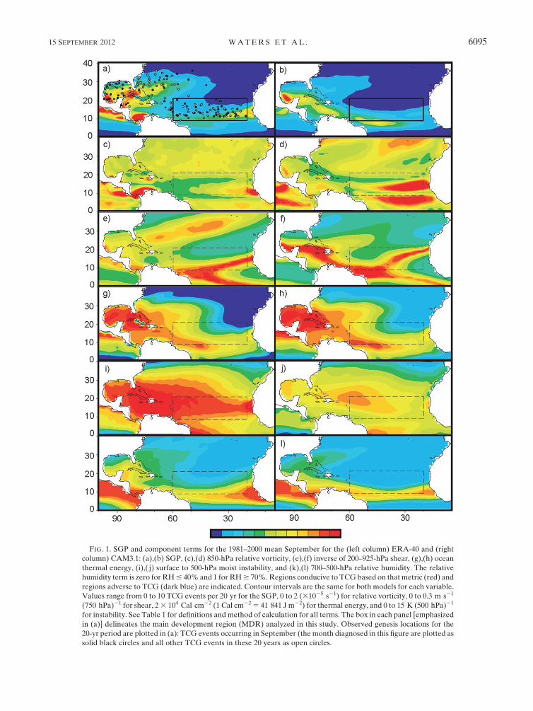
FIG. 1. SGP and component terms for the 1981–2000 mean September for the (left column) ERA-40 and (right

column) CAM3.1: (a),(b) SGP, (c),(d) 850-hPa relative vorticity, (e),(f) inverse of 200–925-hPa shear, (g),(h) ocean

thermal energy, (i),( j) surface to 500-hPa moist instability, and (k),(l) 700–500-hPa relative humidity. The relative

humidity term is zero for RH# 40% and 1 for RH$ 70%.Regions conducive to TCGbased on that metric (red) and

regions adverse to TCG (dark blue) are indicated. Contour intervals are the same for both models for each variable.

Values range from 0 to 10 TCG events per 20 yr for the SGP, 0 to 2 (31025 s21) for relative vorticity, 0 to 0.3 m s21

(750 hPa)21 for shear, 23 104 Cal cm22 (1 Cal cm225 41 841 J m22) for thermal energy, and 0 to 15 K (500 hPa)21

for instability. See Table 1 for definitions and method of calculation for all terms. The box in each panel [emphasized

in (a)] delineates the main development region (MDR) analyzed in this study. Observed genesis locations for the

20-yr period are plotted in (a): TCG events occurring in September (the month diagnosed in this figure are plotted as

solid black circles and all other TCG events in these 20 years as open circles.


in excess of 268C to a depth of 60 m, 2) moist instability

(›ue/›p) for difference in equivalent potential temper-

ature between the surface and 500 hPa, and 3) relatively

high midtroposphere relative humidity (RH). Three

dynamic variables characterize the ability of an incipient

disturbance to focus the latent heating resulting from

this convection: 1) relative vorticity from the surface to

850-hPa (zr), 2) latitudinal Coriolis parameter ( f ), and

3) the inverse of the vertical shear of the horizontal

winds over the depth of the free troposphere between

925 and 200 hPa (S21z ). Gray defined the SGP as

SGP5 (jzrj1 5)jf j

1

Sz1 3

! ðrwcw(T2 26) dz

� �

3

��›ue›p

�1 5

��RH2 40

30

�. (1)

The SGP captures the seasonality and relative frequencies

of TCGacross all major ocean basins (Gray 1979) and has

been used to trace the effects of large-scale interannual

variability (e.g., El Nino) on seasonal TCG frequencies

(Clark and Chu 2002). Several investigations (Ryan

et al. 1992; Watterson et al. 1995; Walsh and Watterson

1997; Royer et al. 1998) have employed the SGP to

evaluate the tropical climate variables relevant for TCG

in control GCM simulations and such inferred potential

changes in TC activity in alternate climate regimes. Such

experiments have highlighted the strong sensitivity of

the SGP to SST through both the ocean thermal energy

and the moist instability parameters.

McBride and Zehr (1981) partitioned the six SGP

terms into two subsets: thermal potential and dynamical

potential for TCG. They noted that only dynamical

parameters possess significant day-to-day variations

throughout a TC season. As a result, they attributed the

SGP thermodynamic parameters to the seasonality of

TCG and the SGP dynamical parameters to daily TCG

potential. They concluded that TCG is a result of large-

scale flow changes in the tropical environment rather

than the properties of the incipient disturbance. These

results helped motivate the medium to high-frequency

diagnostics of large-scale dynamical fields explored here.

Emanuel and Nolan (2004) proposed a genesis po-

tential index [GPI, Eq. (2)] as an advance on the SGP.

The GPI essentially incorporates the same parameters

as the SGP but avoids the ‘‘SST threshold trap’’ by em-

ploying TC potential intensity, denotedVpot, as ameasure

of the thermodynamic support for TCG (Emanuel 1986).

The other parameters incorporated in the GPI are the

850-hPa absolute vorticity (h), 700-hPa relative humid-

ity (H), and 850–200-hPa wind shear of the horizontal

winds (Vshear). An empirical fit to observed TC records

was used to derive the equation defining the nondimen-

sional GPI:

GPI5 j105hj3/2�H

50

�3�Vpot

70

�3(11 0:1Vshear)

22. (2)

The GPI has been used to evaluate the skill of GCMs in

reproducing interannual spatial variations of seasonal

FIG. 2. Observed TCG occurrences within the MDR for each of the 160 15-day base periods

over June–September 1981–2000. The occurrence of at least one TCG event during a particular

15-day period (open bars), and the total number of TCG events that occurred during a par-

ticular 15-day period (solid bars) are shown. This information provides the response variable

for the development of the regression models reported in section 5.


TCG (Camargo et al. 2007; Yokoi et al. 2009) for the

current climate. These GCMs were determined to ex-

hibit skill at reproducing the observed seasonal phasing

and timing of GPI across many oceanic regions; how-

ever, the magnitudes and spatial domains of the GPI

maxima often differed from the validating reanalysis

data.

In section 3a, we employ the SGP andGPI to evaluate

the spatially varying seasonal evolution of the CAM3.1

tropical Atlantic in comparison with the ERA-40.

d. Large-scale diagnostics to infer medium- to high-frequency variability of TCG

Application of the SGP and GPI diagnostics to the

ERA-40 over the 20-yr study period provides spatial

distributions of TCG potential on seasonal time scales

(section 3a). However, recent studies have demonstrated

the importance of the phase of the Madden–Julian os-

cillation (MJO) and equatorial wave activity to medium

to high-frequency TCG variability (e.g., Frank and

Roundy 2006; Aiyyer and Molinari 2008). These struc-

tures in the tropical atmosphere modulate the dynamic

and thermodynamic structure of the large-scale envi-

ronment, impacting the potential for TCG locally in

space and time. While GCMs have shown only limited

skill simulating the MJO (Randall et al. 2007) and moist

equatorial waves (e.g., Straub et al. 2010), consider-

ations of the environmental anomalies associated with

theMJO and equatorial waves informed our selection of

candidate variables designed to capture TCG on time

scales from days to weeks (section 3b, Table 1).

Eleven metrics of the medium to high-frequency

variability of TCG dynamic potential are examined here

(Table 1): 1) the McBride and Zehr (1981) daily genesis

parameter (DGP), defined as the area-integrated dif-

ference between the 925-hPa and 200-hPa relative vor-

ticity; 2) isentropic potential vorticity (IPV) in the lower

troposphere (310 K); 3) upper-troposphere (350 K)

IPV; and 4) the strength of IPV difference between these

two levels. Environmental vertical wind shear is calcu-

lated over three different layers: 5) deep (925–200 hPa)

layer shear, and 6) upper (500–200 hPa)- and 7) lower

(925–500 hPa) tropospheric shear. In addition, moist

IPV (Schubert et al. 2001) is calculated at 8) 310 K

(IPV310-TV) and 9) 350 K (IPV350-TV). The final two

variables calculated are 10) the SGP vorticity parameter

(Gray 1979) and 11) sea level pressure. TCG is more

likely for large values ofDGP, the IPV difference, 310-K

IPV/IPV310-TV, and the SGP vorticity parameter; and

for small values of the 350-K IPV/IPV350-TV, the three

shear parameters, and sea level pressure.

The choice of such thermodynamic TCG metrics is

informed both by concerns with GCM treatments of

moist physics2 and by GCM sensitivities to SST-related

indicators of TCG (e.g., Ryan et al. 1992). The SST

threshold of;268–278C observed for TCG in the current

climate (Evans 1993) appears to be a consequence,

rather than a driver, of the present climate conditions

(Dutton et al. 2000). Thus, it is important to develop

thermodynamic indicators of TCG that are independent

of the absolute value of the underlying SST (although

they may still relate to SST spatial gradients). To mini-

mize concerns about these SST threshold sensitivities,

two parameters designed to capture the convective po-

tential for TCG without reference to SST are examined:

12) daily averaged 500-hPa vertical velocity (W500) and

13) daily averaged convective precipitation rate (PR).

Consistent with the dynamical TCGmetrics, to reference

previous studies, we also analyze two thermodynamic

parameters from the SGP: 14) the moist instability and

15) relative humidity. Two final thermodynamic pa-

rameters are considered: 16) the 500-hPa temperature

at the center of the disturbance and 17) the equivalent

potential temperature at 700 hPa (Table 1).

In summary, 17 metrics of TCG potential on seasonal

andmedium to high-frequency time scales are evaluated

here (Table 1). All metrics are domain averaged over

the MDR and only TCG events occurring in the MDR

are used for validation of these metrics.

e. Calculation of deviation anomalies forintraseasonal metrics of TCG

To assess these TCG variables on medium to high

frequencies, we develop anomalous variability metrics

based on a 15-day base period. We begin by calculating

daily averages of each variable over the MDR to yield

17 time series of daily and spatially averaged variables.

Let r be a 2440 element vector of daily and spatially

averaged values for an arbitrarily chosen variable from

the 17-variable set. To calculate the deviation anoma-

lies, we (i) calculate daily anomalies, rjt ( j5 1, 160; t5 1,

15) of the daily averaged values (elements of the vector r)

compared to the 15-day mean rj, where j indexes over

the set of 15-day time segments3 and t indexes over

individual days within a given time segment. (ii) Standard

deviations (sj) for each 15-day segment of these daily

anomalies are calculated, sj 5 stdev(rjt), and (iii) the

standard deviation s for all of the 15-day periods over

the 20 years is computed via

2 Significant biases in the spatial distribution of precipitation

in the CAM3.1 are evident, even taking into account slight over-

estimates of tropical Atlantic rainfall rates in the ERA-40

(Andersson et al. 2005).3 This analysis spans the 4-month period JJAS for each of the 20

years (1981–2000), so there are 1603 15-day averaging time segments.


s51

N�N

j51

sj, N5 160. (3)

To complete the calculation of the deviation anomaly

time series for the variable r, (iv) we calculate the

standard deviation of the 160 15-day standard deviations

S5 stdv(sj) and, finally, (v) subtract the 20-yr mean

standard deviation s from the set of standard deviations sjand normalize by S to recover the deviation anomalies

s9j 5(sj 2 s)

S, j5 1,160. (4)

Deviation anomalies are designed to highlight anoma-

lous variability in a single time segment (1 # j # 160)

compared to the mean behavior for the set of all 15-day

periods over the 20 years. The deviation anomaly time

series form the basis for comparisons of high-frequency

temporal variations between the ERA-40 and CAM3.1

datasets. They are also used as input into logistic and

Poisson regression models for inference of TCG.

3. Evaluation of CAM3.1 based on existing TCGmetrics

GCM skill in simulation of large-scale environmental

conditions conducive for TCG on monthly and sea-

sonal time scales is still quite variable across models

(Bengtsson et al. 1995, 2007; Camargo et al. 2005). Thus,

it is important to evaluate the skill of the CAM3.1 at

replicating a reasonable spatial distribution of the con-

ditions conducive to TCG before exploring the tropical

high-frequency variability. To do this, we calculate spatial

distributions of the monthly SGP [Eq. (1), Fig. 1] and

monthly GPI [Eq. (2), Fig. 3] from the ERA-40 for

September over the period 1981–2000.

a. Seasonal and monthly time scales: The SGP andGPI

In the first stage of the CAM3.1 validation analysis,

the individual terms and the aggregate values for both

SGP and GPI equations are calculated by month. The

June–September (JJAS) means and September-only

means are used for (i) validation of the diagnostics from

the ERA-40 against the observed TCG record and (ii)

evaluation of the four-member CAM3.1 ensemble. Di-

agnostics of each genesis metric includes evaluations of

their spatial distributions for (i) a single month and year,

(ii) the variance of themonthlymeans, and (iii) the 20-yr

mean and variance. These calculations are performed

for the entire North Atlantic basin, for the MDR alone,

and for a larger tropical band: 98–218N, 208–808W

(Waters 2011). Results for the basinwide and MDR

analyses are reported here.

The SGP fields for the ERA-40 and one of the

CAM3.1 ensemble members4 are comparable in mag-

nitudes (Figs. 1a and 1b). High likelihoods (yellow and

red regions) signifying multiple TCG events are identi-

fied in both the MDR and southern Gulf of Mexico,

but a larger region conducive for TCGevents (the north-

central Atlantic and the majority of the gulf) is evident

in the ERA-40 (Fig. 1a). Further, the TCGmaximum off

equatorial West Africa is well captured in the ERA-40

SGP (Fig. 1a), but in theCAM3.1 thismaximum is shifted

farther west into the central equatorial Atlantic (Fig. 1b).

Comparisons of the SGP component terms (Figs. 1c–l)

provide an explanation for the sources of these discrep-

ancies between the reanalyses and the AGCM. The spa-

tial distributions of the dynamic variables, the scaled

relative vorticity term [Eq. (1); Figs. 1c,d], and the inverse

shear term (Figs. 1e,f) are generally comparable. How-

ever, a small adverse vorticity region in the eastern Ca-

ribbean is noticeable in the ERA-40 that is not present in

the CAM3.1. Similarly, a favorable shear environment in

the north-central Atlantic evident in the ERA-40 is not

replicated in the CAM3.1 simulation. Ocean thermal en-

ergy signatures are also comparable across both models.

The major differences lie in the other thermodynamic

variables: the instability and the RH700–500 parameters.

Although the pattern of moist instability is consistent

between the two (Figs. 1i and 1j), the magnitude of the

CAM3.1 field is substantially weaker. Likewise, CAM3.1

is much drier off of the West African coast, in the

northern gulf, and out into the central North Atlantic. In

summary, the major differences between the CAM3.1

ensemble and ERA-40 (based on the monthly averaged

spatial distributions of SGP diagnostics) are derived from

discrepancies in the thermodynamic parameters.

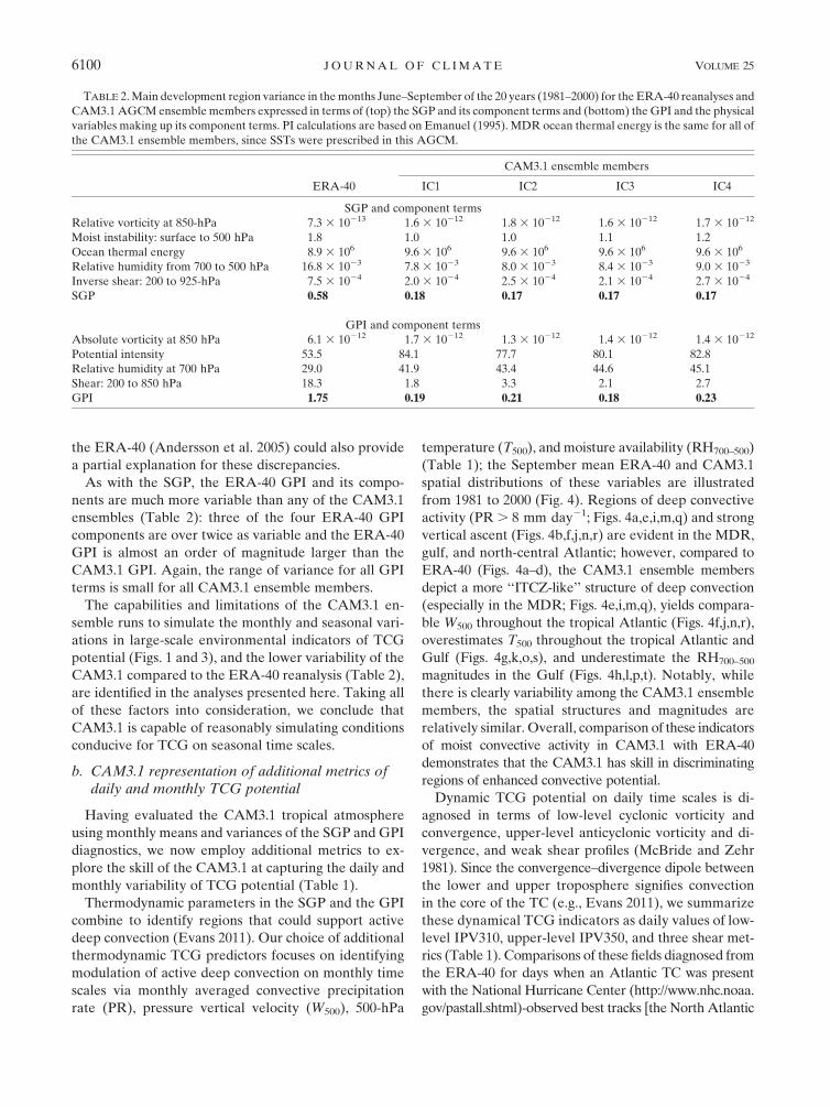
Examination of the variance of the 20-yrMDR-averaged

SGP and each of the SGP component parameters re-

veals that the moist instability, relative humidity, and

shear terms in the ERA-40 are significantly more vari-

able than those in the CAM3.1 ensemble (Table 2).

Overall, the SGP variance in the ERA-40 is triple that

calculated for any of the CAM3.1 ensemble members,

while the four CAM3.1 ensemble members have very

4 The analyses are performed for each of the four ensemble

members. Although each member yields slightly different magni-

tudes of the output variables, noticeable differences are minimal

(Table 2). A comparison of four variables across ERA-40 and all

four ensemble members (Fig. 4) demonstrates that the CAM3.1

results plotted throughout are representative of the ensemble re-

sults more generally. However, for brevity, we generally plot only

one ensemble member.


similar variance ranges for each SGP component; for

instance, variance of the CAM3.1 SGP is only O(0.17–

0.18) compared to 0.58 for the ERA-40 (Table 2).

We also use the GPI [Eq. (2)] and its components (see

ftp://texmex.mit.edu/pub/emanuel/TCMAX/pcmin_revised.f

for the potential intensity routine) to repeat this com-

parison of the monthly averaged conditions conducive

to TCG (Fig. 3). As with the SGP, the spatial distributions

of the dynamical variables, absolute vorticity (Figs. 3c,d),

and shear (Figs. 3e,f) are comparable, although the

CAM3.1 now has slightly stronger shear off West Africa

in addition to the north-central Atlantic (Fig. 3f). Also

consistent with the SGP, the magnitude of the thermo-

dynamic relative humidity parameter is weaker for the

CAM3.1 with drier RH (Fig. 3j) compared to the ERA-40

(Fig. 3i). Potential intensity (PI) output from both ERA-40

(Fig. 3g) andCAM3.1 (Fig. 3h) simulations are comparable.

A tropical precipitation bias that has been identified in

FIG. 3. GPI and component terms for the 1981–2000 mean September: (a),(b) GPI output (number of potential

TCG events totaled over the 20 Septembers), (c),(d) 850-hPa absolute vorticity parameter (s21), (e),(f) 200–850-hPa

shear parameter (m s21), (g),(h) potential intensity (PI) parameter (m s21), and (i),( j) 700-hPa relative humidity

parameter (%). GPI values range from 0 to 10, absolute vorticity values from 0 to 10 (31025 s21), shear magnitudes

from 0 to 20 m s21, PI values up to 20 m s21, and RH values from 0% to 80%. Lower numbers (blue shading)

indicate the least favorable conditions for TCG events and higher numbers (orange and red) indicate the most

favorable conditions for TCG events. The MDR and TCG locations are plotted as described for Fig. 1.


the ERA-40 (Andersson et al. 2005) could also provide

a partial explanation for these discrepancies.

As with the SGP, the ERA-40 GPI and its compo-

nents are much more variable than any of the CAM3.1

ensembles (Table 2): three of the four ERA-40 GPI

components are over twice as variable and the ERA-40

GPI is almost an order of magnitude larger than the

CAM3.1 GPI. Again, the range of variance for all GPI

terms is small for all CAM3.1 ensemble members.

The capabilities and limitations of the CAM3.1 en-

semble runs to simulate the monthly and seasonal vari-

ations in large-scale environmental indicators of TCG

potential (Figs. 1 and 3), and the lower variability of the

CAM3.1 compared to the ERA-40 reanalysis (Table 2),

are identified in the analyses presented here. Taking all

of these factors into consideration, we conclude that

CAM3.1 is capable of reasonably simulating conditions

conducive for TCG on seasonal time scales.

b. CAM3.1 representation of additional metrics ofdaily and monthly TCG potential

Having evaluated the CAM3.1 tropical atmosphere

using monthly means and variances of the SGP and GPI

diagnostics, we now employ additional metrics to ex-

plore the skill of the CAM3.1 at capturing the daily and

monthly variability of TCG potential (Table 1).

Thermodynamic parameters in the SGP and the GPI

combine to identify regions that could support active

deep convection (Evans 2011). Our choice of additional

thermodynamic TCG predictors focuses on identifying

modulation of active deep convection on monthly time

scales via monthly averaged convective precipitation

rate (PR), pressure vertical velocity (W500), 500-hPa

temperature (T500), and moisture availability (RH700–500)

(Table 1); the September mean ERA-40 and CAM3.1

spatial distributions of these variables are illustrated

from 1981 to 2000 (Fig. 4). Regions of deep convective

activity (PR. 8 mm day21; Figs. 4a,e,i,m,q) and strong

vertical ascent (Figs. 4b,f,j,n,r) are evident in the MDR,

gulf, and north-central Atlantic; however, compared to

ERA-40 (Figs. 4a–d), the CAM3.1 ensemble members

depict a more ‘‘ITCZ-like’’ structure of deep convection

(especially in the MDR; Figs. 4e,i,m,q), yields compara-

ble W500 throughout the tropical Atlantic (Figs. 4f,j,n,r),

overestimates T500 throughout the tropical Atlantic and

Gulf (Figs. 4g,k,o,s), and underestimate the RH700–500

magnitudes in the Gulf (Figs. 4h,l,p,t). Notably, while

there is clearly variability among the CAM3.1 ensemble

members, the spatial structures and magnitudes are

relatively similar. Overall, comparison of these indicators

of moist convective activity in CAM3.1 with ERA-40

demonstrates that the CAM3.1 has skill in discriminating

regions of enhanced convective potential.

Dynamic TCG potential on daily time scales is di-

agnosed in terms of low-level cyclonic vorticity and

convergence, upper-level anticyclonic vorticity and di-

vergence, and weak shear profiles (McBride and Zehr

1981). Since the convergence–divergence dipole between

the lower and upper troposphere signifies convection

in the core of the TC (e.g., Evans 2011), we summarize

these dynamical TCG indicators as daily values of low-

level IPV310, upper-level IPV350, and three shear met-

rics (Table 1). Comparisons of these fields diagnosed from

the ERA-40 for days when an Atlantic TC was present

with the National Hurricane Center (http://www.nhc.noaa.

gov/pastall.shtml)-observed best tracks [the NorthAtlantic

TABLE 2.Main development region variance in themonths June–September of the 20 years (1981–2000) for the ERA-40 reanalyses and

CAM3.1 AGCMensemblemembers expressed in terms of (top) the SGP and its component terms and (bottom) the GPI and the physical

variables making up its component terms. PI calculations are based on Emanuel (1995). MDR ocean thermal energy is the same for all of

the CAM3.1 ensemble members, since SSTs were prescribed in this AGCM.

ERA-40

CAM3.1 ensemble members

IC1 IC2 IC3 IC4

SGP and component terms

Relative vorticity at 850-hPa 7.3 3 10213 1.6 3 10212 1.8 3 10212 1.6 3 10212 1.7 3 10212

Moist instability: surface to 500 hPa 1.8 1.0 1.0 1.1 1.2

Ocean thermal energy 8.9 3 106 9.6 3 106 9.6 3 106 9.6 3 106 9.6 3 106

Relative humidity from 700 to 500 hPa 16.8 3 1023 7.8 3 1023 8.0 3 1023 8.4 3 1023 9.0 3 1023

Inverse shear: 200 to 925-hPa 7.5 3 1024 2.0 3 1024 2.5 3 1024 2.1 3 1024 2.7 3 1024

SGP 0.58 0.18 0.17 0.17 0.17

GPI and component terms

Absolute vorticity at 850 hPa 6.1 3 10212 1.7 3 10212 1.3 3 10212 1.4 3 10212 1.4 3 10212

Potential intensity 53.5 84.1 77.7 80.1 82.8

Relative humidity at 700 hPa 29.0 41.9 43.4 44.6 45.1

Shear: 200 to 850 hPa 18.3 1.8 3.3 2.1 2.7

GPI 1.75 0.19 0.21 0.18 0.23


hurricane database (HURDAT)] confirms that the

ERA-40 diagnostics are reasonable metrics for daily

TCG potential.

The 20-yr simulation of the CAM3.1 cannot be expec-

ted to validate in day-by-day comparisons but should

produce spatial patterns and modes of variability consis-

tent with the observed local weather and climate. Com-

parisons of these daily dynamical metrics from CAM3.1

with ERA-40 (not shown) reveal that the magnitudes of

the shear terms and IPV350 are similar between the two.

CAM3.1 develops low-level vortices of similar spatial

scales to those analyzed in ERA-40, but the magnitudes

of these IPV310 signatures are smaller.

4. Principal component analysis on subseasonalTCG data

To focus on the variability of the large-scale environ-

ment as the signature of TCG, we calculate deviation

anomalies averaged over the entire MDR (section 2e)

for each baseline 15-day period. These deviation anoma-

lies are calculated for the ERA-40 and each of the

CAM3.1 ensemble members for all 17 candidate vari-

ables (Table 1). We perform principal component anal-

ysis (e.g., Von Storch and Zwiers 1999) on a correlation

matrix created from the vector x of deviation anomalies

calculated for all input variables. This approach is de-

signed to remove redundancies among the input variable

set and to develop a reduced set of orthogonal composite

principal component (PC) vectors to use as inputs to the

new TCG summary metrics described in section 5. Each

PC is defined by an eigenvector comprising elements

(loading values) that are linear combinations of x (Wilks

2006, 463–466). Thus, the mth PC um is the projection of

x onto the mth eigenvector em:

um 5 eTmx5 �K

k51

ekmxk, m5 1, . . . ,M . (5)

Here, each of the M eigenvectors contains one loading

value pertaining to each of the K variables, xk. The first

eigenvector points in the direction in which x exhibits

the most joint temporal variability. Subsequent eigen-

vectors are perpendicular to all previous eigenvectors

and locate directions in which the original data displays

maximum remaining joint temporal variability. Thus, all

PCs are mutually uncorrelated and account successively

for the maximum joint variability of x. We retain the

subset of PCs for the ERA-40 and additional PC subsets

for each CAM3.1 ensemblemember that explain at least

70% of the combined variance.

FIG. 4. Comparison of 1981–2000 monthly averaged September thermodynamic metrics (Table 1) for (top row) ERA-40 and (lower

rows) each of theCAM3.1 ensemblemembers: (from left to right) convective precipitation rate (PR,mm day21), 500-hPa vertical velocity

W500 (hPa day21), 500-hPa temperature T500 (K), and midtropospheric relative humidity RH700–500 (%).


The loading values in each PC (plotted by variable for

the ERA-40 and each of the four CAM3.1 ensemble

members in Fig. 5) are examined to determine the domi-

nant dynamic and/or thermodynamic contributors to each

PC. Having established the dominant contributors to each

PC, we examine the dominant contributors to each PC

for the ERA-40 and the CAM3.1 ensemble members to

compare their dominant sources of variability in theMDR.

Intercomparison of the variables in ERA-40 and

CAM3.1 dominating the variance explained by the in-

dividual PCs provides insights into the sources for the

discrepancies highlighted by the SGP (Fig. 1) and GPI

(Fig. 3) diagnostics. PC1 and PC2 show similar de-

pendencies across all ERA-40 and CAM3.1 analyses,

but there is less consistency of variable contributions to

PC3 through PC7 (Fig. 5). The first PC of the ERA-40

FIG. 5. Variable loadings for each of the first seven principal components (color coded)

diagnosed in (a) the ERA-40 and (b)–(e) the four CAM3.1 ensemble members. An individual

PC is constructed bymultiplying the value indicated by the corresponding bar with the variable

and summing across all variables to recover the linear combination as given in Eq. (5);

(f) percent variance explained for each PC for (from left to right) the ERA-40 and each

CAM3.1 ensemble members are plotted.


captures variability in the upper-level IPV (IPV350,

IPV350-Tv, and IPVDiff) and shear (Shear200–500,

Shear500–925, and Shear200–925) terms. The effects

of convection are evident in PC2 via PR and W500 and

indirectly through z850, which will act to reduce the

Rossby radius and, thus, enhance the effects of the

convection locally. Although these ERA-40 depen-

dencies for PC1 and PC2 are generally repeated in

each of the CAM3.1 ensemble members, some differ-

ences are evident. For example, all CAM3.1 members

have similar loading values for the DGP and all five

IPV terms in PC1, indicating a notable inability of

the CAM3.1 to differentiate between upper-level and

lower-level dynamic rotational variability. Similarly,

in PC2 all CAM3.1 members identify the dominant

covariance between PR and W500 but do not capture a

link to z850.

Dynamic terms dominate the weaker PCs retained

(PC3–PC7) for the ERA-40, with the thermodynamic

terms playing a supporting role at best. PC3 is most

influenced by IPV in the upper troposphere, while

PC4 captures lower-tropospheric IPV variability, with a

weaker (negative) dependence on the moisture vari-

ables RH700–500 and ThetaE700. PC5 has the strongest

contribution from the DGP, but once again RH700–500

and ThetaE700 play a supporting role. SLP provides a

major influence on PC6, but the DGP is also a strong

contributor, with the convective terms PR andW500 also

contributing to the variance explained by this PC. The

variability in PC7 is dominated by SLP.

The CAM3.1 PC3–PC7 yield a more uniform distribu-

tion of similar dynamic and thermodynamic terms. Three

of the four members capture the dominant variability and

covariability of the dynamic terms (i.e., IPV terms,

SLP) evident in the ERA-40, but the thermodynamic

variables—ThetaE700, instability, and RH700–500—that

contributed weakly to the ERA-40 PC play a much

stronger role here. These results suggest that the ther-

modynamic terms vary more on the 15-day time scale

in CAM3.1 than in ERA-40.

Results from this analysis indicate several important

capabilities and limitations of the CAM3.1 for capturing

subseasonal MDR variability. All CAM3.1 members

exhibit similar dependencies (variable loadings) to the

ERA-40 for PC1 and PC2. However, the CAM3.1 en-

semble members uniformly capture a stronger contri-

bution of the thermodynamic terms in PC3–PC7 and

downplay the influence of other dynamic variables, such

as DGP and SLP, in explaining temporal variability on

the 15-day time scale within the MDR. The variance

explained by PC1 in all CAM3.1 members is much

higher than that for the ERA-40, consistent with the

reduced variability in this AGCM (Table 2).

5. Development of regression models for TCG inthe MDR

The resolution of the CAM3.1 simulations analyzed

here (1.48 3 1.48) is too coarse to capture the details of

genesis, so we need to infer TC activity from the GCM

fields. The distinction between this study and earlier

works of this kind is that the composite metrics de-

veloped here directly incorporate measures of daily

anomalous variability within 15-day periods (section 2e)

of each variable of interest. Using the first seven PCs

calculated from the PCA applied to the ERA-40 large-

scale fields (section 4), we develop two regression

models to assess how well the high-frequency variability

is associated with (i) observed TCG events ($1; logistic

regression model) and (ii) multiple observed TCG

events ($1, Poisson regression model) within the MDR

domain in a given 15-day time period. The seven PCs

are chosen because they explain a sufficient amount of

temporal variance of the original deviation anomalies

that we deemed appropriate. Furthermore, this choice

of employing the PCs as the predictor set reflects our

initial hypothesis that information on short-time-scale

variability is necessary for skillful TCG detection. Thus,

the skill of these regression models provides informa-

tion on the relative importance of measures of high-

frequency variability in detecting TCGwithin theMDR.

This regression method is not a predictive tool, but a

step toward developing a diagnostic for inferring TCG

likelihood in GCMs that utilizes variability metrics

of the genesis environment. We do not create regres-

sion models based on the CAM3.1 because to do so we

would have needed to simulate TCG and TC events

within the AGCM, which strays from the goals of this

paper. However, given the CAM3.1 skill in simulating

seasonality and medium- to high-frequency variability

signatures (sections 3 and 4), we hypothesize that a

regression model determined from the ERA-40 could

be applied to the CAM3.1 to infer TCG likelihoods.

We report on the results from both regression models

here.

a. Logistic regression using reanalysis data

We first develop a logistic regression model to assess

the diagnostic capabilities of the ERA-40-based PCs

(predictors) to detect observed TCG occurrences (pre-

dictand, Fig. 2) on the 15-day time scales. In the process

of logistic regression, we fit a logit probability func-

tion, pi 5 (11 e2zi)21, i5 1, N, where N is the number

of 15-day time periods, using logistic regression to the

predictors xk (the seven leading PCs) for a known set of

outcomes Zi [the binary predictand: TCG yes (Y) or no

(N; see Fig. 2] by maximizing the log-likelihood


ln

�pi

12 pi

�5 b01 b1x1i 1 � � � 1 bk xki 5Zi , (6)

where (b0, b1, b2, . . . , bk) are the regression parameters.

Using this technique, the regression estimates become

bounded on the interval [0, 1] in the form of an S-shaped

curve (Fig. 6).

To evaluate our logistic regression model, we de-

termine that genesis will be detected for p$ 0.5 and will

not be detected for p, 0.5. We summarize these results

in a 23 2 confusion matrix (inset in Fig. 6). A variety of

skill metrics can be evaluated (Wilks 2006) from the

information summarized in the confusion matrix: we

employ accuracy, precision, threat score, and hit rate to

evaluate this model (Table 3).

The logistic regressionmodel (Fig. 6) correctly detects

(YY or NN in the confusion matrix) 131 of the 160

events, yielding an accuracy of 82%. Similarly, 21 of the

27 TCG predictions are verified, corresponding to a

model precision of 78%. Based on these statistics, the

model appears to be performing at an exemplary level.

However, threat score and hit rate also take into account

false alarms (Table 3) and thus provide a more rigorous

test of model skill. This model achieves a threat score of

42% and hit rate of 48%. So, even by the most stringent

skill metrics commonly used, this large-scale variability-

based model correctly identifies TCG occurrences in the

period almost 50% of the time.

b. Poisson regression

A Poisson regression model was developed to de-

termine the diagnostic capabilities of high-frequency

variability at detecting multiple TCG events in a 15-day

window (Fig. 7). Using the same seven ERA-40 PCs as

predictors, we calculate the conditional mean mi of the

predictand (number of events); mi, modeled as a Poisson

random variate dependent on the seven PC predictors fit

to the predictand of genesis, counts using the same log-

likelihood method for estimation of the fitting parame-

ters as employed for the logistic regression [Eq. (6)]. To

FIG. 6. Performance of the TCG logistic regression model based on 15-day deviation

anomalies from the ERA-40. Observed genesis (or nongenesis) events (open circles); the re-

sulting logistic regression model indicating the likelihood of a TCG occurrence for a given

value of Z (derived from the large-scale deviation anomalies) is plotted (asterisk line). The

inset is the confusion matrix summary of these results. The confusion matrix statistics are

compiled using a threshold probability of 0.5 to designate a TCG event forecast by the re-

gression model.

TABLE 3. Skill metrics used in the evaluation of the logistic and

Poisson regressionmodels. Statistics for the outcomes are provided

in the confusion matrix inset in Figs. 6 and 7. Outcomes are in-

terpreted as YY: TCG is forecast and observed, YN: TCG is

forecast but does not occur (false alarm), NY: TCG is observed but

is not forecast (miss), and NN: TCG is not forecast and does not

occur.

Skill metric Definition

Accuracy Proportion of correct predictions

from all predictions

Precision Proportion of correct positives from

all positive predictions

Skill score Proportion of correct true forecasts

from all occasions that event was

either forecasted or observed

Threat rate Proportion of correct true forecasts

to the number of events observed


evaluate the Poissonmodel skill at identifying a plurality

of TCG events, we construct a 33 3 confusionmatrix for

TCG count ranges 0, 1, .1. As with the logistic re-

gression model, TCG was determined to be detected if

the number of projected occurrences exceeded 0.5 and

the forecast TCG count was incremented at 1.5 (two

events), 2.5 (three events), and 3.5 (four events); no 15-day

period had more than four events.

Threat score and hit rate data indicate a weak pre-

dictive skill of the PC combinations to detect observed

TCG counts in a given 15-day period: threat scores and

hit rates are comparable for the non TCG (67% and

96%) and single TCG occurrences (16% and 24%), but

improved for TCG counts greater than one (28% and

29%). Although the computed threat scores are not ro-

bust, actual TCG counts were within one of the projected

TCG counts (96%). These findings suggest that the

Poisson approach has the potential for increased skill if a

larger TCG count database is employed, but overall

weaker skill than the logistic regression (Figs. 6 and 7).

6. Summary and conclusions

In this study, we assess the capabilities of an atmo-

spheric GCM for detecting both large-scale and localized

conditions for genesis in the tropical North Atlantic. We

develop metrics of medium- to high-frequency (15-day

base period) variability of environmental conditions and

assess their utility as diagnostics of TCG in the North

Atlantic MDR. We explore the hypothesis that inclusion

of information on variability, especially of the dy-

namic fields, will provide improved diagnostics of TCG.

Diagnostics of high-frequency variability in the dy-

namical fields provide information on the development

of potential incipient vortices as centers for TCG de-

velopment.

Seventeen candidate thermodynamic and dynamic

variables are identified as potential indicators of TCG

activity. A four-member ensemble of the CAM3.1

atmospheric GCM is compared with observed TCG

activity from 1981 to 2000 and with TCG variability

metrics diagnosed from the ERA-40 dataset. The

CAM3.1 is forced with observed monthly sea surface

temperatures for the 20-yr period. Overall, CAM3.1

exhibits skill at simulating large-scale and localized

TCG environments. Based on principal component

analysis applied to CAM3.1 and ERA-40 data, CAM3.1

data exhibit distinct differences from ERA-40 data.

Most of the temporal variability in the ERA-40 is ex-

plained by dynamic variability. This dominance of high-

frequency variability in the dynamic fields is consistent

with our hypothesis that metrics of TCG must capture

information on the development of potential incipient

vortices for TCG development. Although all CAM3.1

members exhibit similar primary dependencies on dy-

namic variability, they uniformly capture a stronger sub-

sequent contribution of the thermodynamic terms and

downplay the influence of other dynamic variables in

explaining temporal variability on the 15-day time scale

within the MDR.

FIG. 7. Performance of the TCG Poisson regression model based on 15-day deviation

anomalies from the ERA-40. Observed genesis (or nongenesis) events (open circles), and the

Poisson regressionmodel indicating the number of TCG events likely to occur for a given value

of Z (derived from the large-scale deviation anomalies) is plotted as asterisks. The inset is the

confusion matrix summary of these results. The confusionmatrix statistics are compiled using a

threshold probability of 0.5 to designate a TCG event forecast by the regression model.


We calculate the normalized standard deviation of

daily anomalous variability from a 15-day base period

for each of the 17 TCG predictors; application of PCA

on the results in a set of 17 deviation anomaly time series

reduces the potential indicators to a set of seven un-

correlated principal components (PCs) for TCG likeli-

hood in the 15-day period. These seven ERA-40-based

PCs are used as predictors in a logistic regression model

for detection of TCG activity in the MDR. The logistic

regression model yields promising accuracy (82%) and

precision (78%) measures, achieving a threat score of

42% and a hit rate of 48%.

Because multiple TCG events in a given base period

result in higher magnitudes of variability for that period,

we develop a Poisson regression model for TCG counts

based on the same seven predictors. Threat scores and

hit rates for TCG counts of at least one TCG event are

lower (31% and 27%, respectively) than the logistic

regressionmodel, demonstrating that weighting by TCG

counts does not improve the regression model skill.

Based on these findings, there is merit in incorporating

a measure of medium- to high-frequency variability (daily

deviations from a 15-day base period) in metrics of TCG.

The logistic regression model developed here may pro-

vide a useful tool in seasonal forecasting of TCG activity

given a seasonal forecast (or ensemble of forecasts) from a

dynamical numerical model. Further, given a climate

model with skillful representation of seasonal and

monthly large-scale environmental metrics of TCG, the

logistic regressionmodel could provide a useful diagnostic

of TCG likelihood.

Acknowledgments. This work was funded by the Na-

tional Science Foundation under Grant ATM-0735973.

We are grateful to Dr. Wei Li for her help in performing

the CAM3.1 simulations. Chuck Pavloski and Chad

Bahrmann provided excellent programming assistance

and scientific database management.

REFERENCES

Aiyyer, A., and J. Molinari, 2008:MJO and tropical cyclogenesis in

the Gulf of Mexico and Eastern Pacific: Case study and ide-

alized numerical modeling. J. Atmos. Sci., 65, 2691–2704.

Andersson, E., and Coauthors, 2005: Assimilation and modeling of

the atmospheric hydrological cycle in theECMWF forecasting

system. Bull. Amer. Meteor. Soc., 86, 387–402.

Bengtsson, L., H. Bottger, and M. Kanamitsu, 1982: Simulation of

hurricane-type vortices in a general circulation model. Tellus,

34, 440–457.

——, M. Botzet, and M. Esch, 1995: Hurricane-type vortices in

a general circulation model. Tellus, 47A, 175–196.——, K. I. Hodges, M. Esch, N. Keenlyside, L. Kornblueh, J.-J. Luo,

and T. Yamagata, 2007: How may tropical cyclones change in

a warmer climate? Tellus, 59A, 539–561.

Camargo, S. J., and A. H. Sobel, 2004: Formation of tropical

storms in an atmospheric general circulation model. Tellus,

56A, 56–67.

——, A. G. Barnston, and S. E. Zebiak, 2005: A statistical assess-

ment of tropical cyclone activity in atmospheric general cir-

culation models. Tellus, 57A, 589–604.——, A. H. Sobel, A. G. Barnston, and K. A. Emanuel, 2007:

Tropical cyclone genesis potential index in climate models.

Tellus, 59A, 428–443.

Challa, M., and R. L. Pfeffer, 1990: Formation of Atlantic hurri-

canes from cloud clusters and depressions. J. Atmos. Sci., 47,

909–927.

Charney, J. G., and A. Eliassen, 1964: On the growth of the hur-

ricane depression. J. Atmos. Sci., 21, 68–75.

CISL, cited 2011: Computational and Information Systems Labo-

ratory (CISL) Research Data Archive. [Available online at

http://dss.ucar.edu/.]

Clark, J. D., and P. S. Chu, 2002: Interannual variation of tropical

cyclone activity over the central North Pacific. J. Meteor. Soc.

Japan, 80, 403–418.Collins, W. D., G. B. Bonan, T. B. Henderson, andD. S. McKenna,

2004: The Community Climate System Model: CCSM3.

J. Climate, 17, 1–30.

Dutton, J. F., C. J. Poulsen, and J. L. Evans, 2000: The effect of

global climate change on the regions of tropical convection in

CSM1. Geophys. Res. Lett., 27, 3049–3052.

ECMWF, cited 2011: ERA-40 background. [Available at http://

www.ecmwf.int/research/era/do/get/era-40.]

Emanuel, K. A., 1986: An air–sea interaction theory for tropical

cyclones. Part I: Steady-state maintenance. J. Atmos. Sci., 43,

585–605.

——, 1995: Sensitivity of tropical cyclones to surface exchange

coefficients and a revised steady-state model incorporating

eye dynamics. J. Atmos. Sci., 52, 3969–3976.

——, and D. Nolan, 2004: Tropical cyclone activity and global

climate. Preprints, 26th Conf. on Hurricanes and Tropical

Meteorology, Miami, FL, Amer. Meteor. Soc., 10A.2. [Avail-

able online at https://ams.confex.com/ams/pdfpapers/75463.

pdf.]

——, R. Sundararajan, and J. Williams, 2008: Hurricanes and

global warming: Results from downscaling IPCC AR4 simu-

lations. Bull. Amer. Meteor. Soc., 89, 347–367.

Evans, J. L., 1993: Sensitivity of tropical cyclone intensity to sea

surface temperature. J. Climate, 6, 1133–1140.

——, 2011: Chapter 8: Tropical cyclones. Introduction to Tropical

Meteorology, version 2.0, A. Laing and J. L. Evans, Eds.,

COMET. [Available online at http://www.meted.ucar.edu/

tropical/textbook_2nd_edition/index.htm.]

Frank,W.M., and P. E. Roundy, 2006: The role of tropical waves in

tropical cyclogenesis. Mon. Wea. Rev., 134, 2397–2417.Gall, J. S., I. Ginis, S.-J. Lin, T. P. Marchok, and J.-H. Chen, 2011:

Experimental tropical cyclone prediction using the GFDL

25-km-resolution global atmospheric model. Wea. Forecasting,

26, 1008–1019.

Goldenberg, S. B., and L. J. Shapiro, 1996: Physical mechanisms for

the association of El Nino and West African rainfall with

Atlantic major hurricane activity. J. Climate, 9, 1169–1187.

Gray, W. M., 1968: Global view of the origin of tropical distur-

bances and storms. Mon. Wea. Rev., 96, 669–700.——, 1979: Hurricanes: Their formation, structure and likely role

in the tropical circulation. Meteorology over the Tropical

Oceans, D. B. Shaw, Ed., Royal Meteorological Society,

155–218.


——, 1988: Environmental influences on tropical cyclones. Aust.

Meteor. Mag., 36, 127–138.

Knutson, T.R., J. J. Sirutis, S. T.Garner, I.M.Held, andR.E. Tuleya,

2007: Simulation of the recent multidecadal increase of Atlantic

hurricane activity using an 18-km-grid regional model. Bull.

Amer. Meteor. Soc., 88, 1549–1565.

LaRow, T. E., Y.-K. Lim, D. W. Shin, E. P. Chassignet, and

S. Cocke, 2008: Atlantic basin seasonal hurricane simulations.

J. Climate, 21, 3191–3206.

McBride, J. L., and R. Zehr, 1981: Observational analysis of tropical

cyclone formation. Part II: Comparison of nondeveloping versus

developing systems. J. Atmos. Sci., 38, 1132–1151.McDonnell, K. A., and N. J. Holbrook, 2004: A Poisson regression

model of tropical cyclogenesis for the Australian–southwest

Pacific Ocean region. Wea. Forecasting, 19, 440–455.Montgomery, M. T., and B. F. Farrell, 1993: Tropical cyclone for-

mation. J. Atmos. Sci., 50, 285–310.

Oouchi, K., J. Yoshimura, H. Yoshimura, R. Mizuta, S. Kusunoki,

and A. Noda, 2006: Tropical cyclone climatology in a global-

warming climate as simulated in a 20km-mesh global at-

mospheric model: Frequency and wind intensity analyses.

J. Meteor. Soc. Japan, 84, 259–276.

Ooyama, K., 1964: A dynamical model for the study of tropical

cyclone development. Geofis. Int., 4, 187–198.

Randall, D. A., and Coauthors, 2007: Climate models and their

evaluation. Climate Change 2007: The Physical Science Basis,

S. Solomon et al., Eds., Cambridge University Press, 589–662.

Royer, J.-F., F. Chauvin, B. Timbal, P. Araspin, and D. Grimal,

1998: A GCM study of the impact of greenhouse gas increase

on the frequency of occurrence of tropical cyclones. Climatic

Change, 38, 301–343.

Ryan, B. F., I. G. Watterson, and J. L. Evans, 1992: Tropical cy-

clone frequencies inferred from Gray’s yearly genesis pa-

rameter: Validation of GCM tropical climates. Geophys. Res.

Lett., 19, 1831–1834.

Schubert, W. H., S. A. Hausman, M. Garcia, K. V. Ooyama, and

H.-C. Kuo, 2001: Potential vorticity in a moist atmosphere.

J. Atmos. Sci., 58, 3148–3157.

Smirnov, D., and D. J. Vimont, 2011: Variability of the Atlantic

Meridional Mode during the Atlantic hurricane season.

J. Climate, 24, 1409–1424.Sobel, A. H., E. D. Maloney, G. Bellon, and D. M. Frierson, 2009:

Surface fluxes and tropical intraseasonal variability: A re-

assessment. J. Adv. Model. Earth Syst., 2, 1–27.

Straub, K. H., P. T. Haertel, and G. N. Kiladis, 2010: An analysis of

convectively coupledKelvin waves in 20WCRPCMIP3 global

coupled climate models. J. Climate, 23, 3031–3056.

Thorncroft, C., and I. Pytharoulis, 2001: A dynamical approach to

seasonal prediction of Atlantic tropical cyclone activity. Wea.

Forecasting, 16, 725–734.

Vecchi, G. A., and B. J. Soden, 2007: Increased tropical Atlantic

wind shear in model projections of global warming. Geophys.

Res. Lett., 34, L08702, doi:10.1029/2006GL028905.

——,M.Zhao,H.Wang,G.Villarini,A.Rosati,A.Kumar, I.M.Held,

and R. Gudgel, 2011: Statistical–dynamical predictions of

seasonal North Atlantic hurricane activity. Mon. Wea. Rev.,

139, 1070–1082.

Vitart, F., 2006: Seasonal forecasting of tropical storm frequency

using a multi-model ensemble. Quart. J. Roy. Meteor. Soc.,

132, 647–666.

——, J. L. Anderson, and W. F. Stern, 1997: Simulation of in-

terannual variability of tropical storm frequency in an en-

semble of GCM integrations. J. Climate, 10, 745–760.

——, and Coauthors, 2007: Dynamically-based seasonal fore-

casts of Atlantic tropical storm activity issued in June by

EUROSIP. Geophys. Res. Lett., 34, L16815, doi:10.1029/

2007GL030740.

Von Storch, H., and F. W. Zwiers, 1999: Statistical Analysis in

Climate Research. Cambridge University Press, 495 pp.

Walsh, K., and I. G.Watterson, 1997: Tropical cyclone-like vortices

in a limited area model: Comparison with observed climatol-

ogy. J. Climate, 10, 2240–2259.

Waters, J., 2011: Towards improving the detection of North

Atlantic tropical cyclogenesis (TCG). M.S. thesis, Depart-

ment of Meteorology, The Pennsylvania State University,

112 pp.

Watterson, I. G., J. L. Evans, and B. F. Ryan, 1995: Seasonal and

interannual variability of tropical cyclogenesis: Diagnostics

from large scale fields. J. Climate, 8, 3052–3065.

Wehner, M. F., G. Bala, P. Duffy, A. A. Mirin, and R. Romano,

2010: Towards direct simulation of future tropical cyclone

statistics in a high resolution global atmospheric model. Adv.

Meteor., 2010, 915303, doi:10.1155/2010/915303.

Wilks, D. S., 2006: Statistical Methods in the Atmospheric Sciences.

2nd ed. Elsevier, 627 pp.

Yokoi, S., Y. N. Takayabu, and J. C.-L. Chan, 2009: Tropical cyclone

genesis frequency over the western North Pacific simulated

in medium-resolution coupled general circulation models.

Climate Dyn., 33, 665–683.

Zhang, Y., S. Klein, J. Boyle, andG. G.Mace, 2010: Evaluation of

tropical cloud and precipitation statistics of Community At-

mosphere Model version 3 using CloudSat and CALIPSO data.

J. Geophys. Res., 115, D12205, doi:10.1029/2009JD012006.

Zhao, M., and I. M. Held, 2010: An analysis of the effect of global

warming on the intensity of Atlantic hurricanes using a GCM

with statistical refinement. J. Climate, 23, 6382–6393.

——,——, S.-J. Lin, and G. A. Vecchi, 2009: Simulations of global

hurricane climatology, interannual variability, and response to

global warming using a 50-km resolution GCM. J. Climate, 22,6653–6678.


Large-Scale Diagnostics of Tropical Cyclogenesis … Diagnostics of Tropical Cyclogenesis Potential...

Documents

Transcript of Large-Scale Diagnostics of Tropical Cyclogenesis … Diagnostics of Tropical Cyclogenesis Potential...