Large Scale Circuit Placement: Gap and Promise -...

Large Scale Circuit Placement: Gap and Promise

Jason Cong1, Tim Kong2, Joseph R. Shinnerl1, Min Xie1 and Xin Yuan1

UCLA VLSI CAD LAB1

Magma Design Automation2

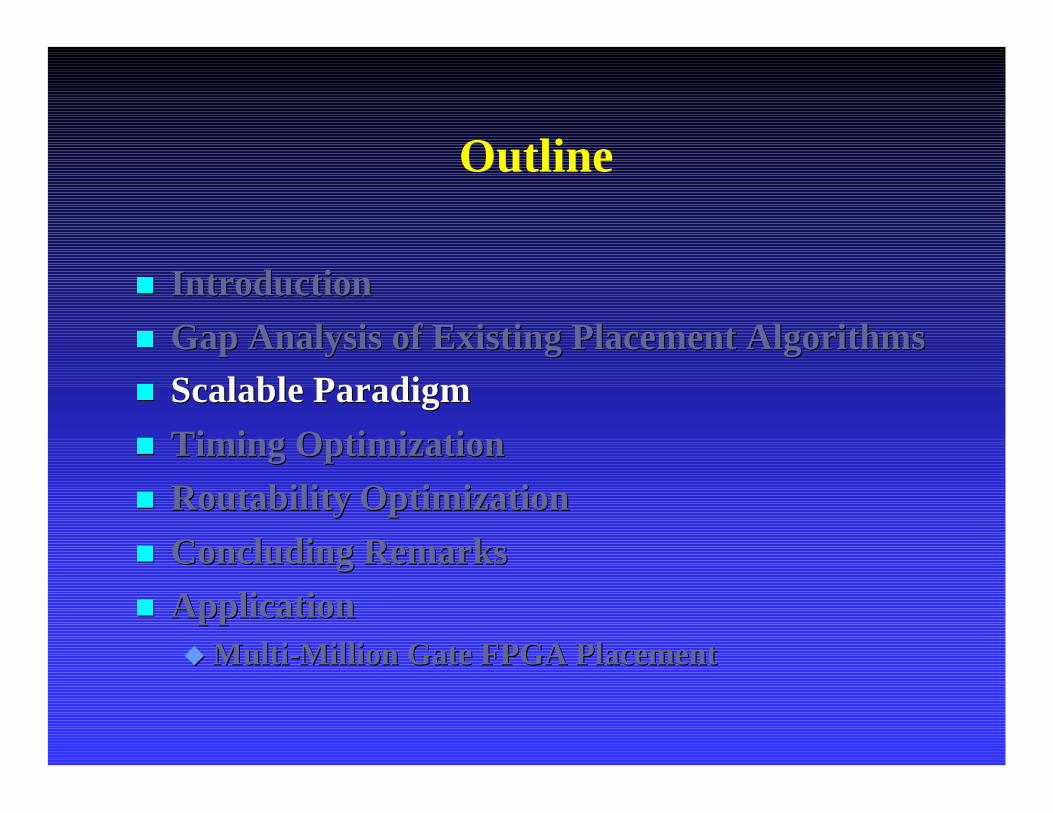
Outline

n Introductionn Gap Analysis of Existing Placement Algorithmsn Scalable Paradigmn Timing Optimizationn Routability Optimizationn Concluding Remarksn ApplicationuMulti-Million Gate FPGA Placement

Outline

nn IntroductionIntroductionnn Gap Analysis of Existing Placement AlgorithmsGap Analysis of Existing Placement Algorithmsnn Scalable ParadigmScalable Paradigmnn Timing OptimizationTiming Optimizationnn RoutabilityRoutability OptimizationOptimizationnn ConcludingConcluding RemarksRemarksnn Application Application uuMultiMulti--Million Gate FPGA PlacementMillion Gate FPGA Placement

Why Still Placement Problem

n True, it has been studied over 30 years, but …n We need good solutions more then ever

u One of most important steps in IC implementation flowF Directly defines interconnects

n Difficultu Problem size grows 2X every 18-24 months

F Moore’s Law

u Cannot place hierarchically without quality degradation

Example of Logic Hierarchy in Final Layout

By courtesy of IBM (Tony Drumm)

Why Still Placement

n True, it has been studied over 30 years, but …n We need good solutions more then ever

u One of most important steps in IC implementation flowF Directly defines interconnects

n Difficultu Problem size grows 2X every 18-24 months

F Moore’s Law

u Cannot place hierarchically without quality degradation

n We are not very good at it …

Outline

nn IntroductionIntroductionnn Gap Analysis of Existing Placement AlgorithmsGap Analysis of Existing Placement Algorithmsnn Scalable ParadigmScalable Paradigmnn Timing OptimizationTiming Optimizationnn RoutabilityRoutability OptimizationOptimizationnn ConcludingConcluding RemarksRemarksnn ApplicationApplicationuuMultiMulti--Million Gate FPGA PlacementMillion Gate FPGA Placement

Motivation

n Lack of significant progress in wirelength reductionuRate of reduction is about 5-10% every 2-3 yearsuLatest developments in placement differ mainly in

runtime

n Most work compare only with known heuristicsuUse real design based benchmarksuUse synthetic benchmarks

n Little understanding about the divergence from the optimal

Placement Examples with Known Optimal Wirelength [Chang et al, 2003]

n All the modules are of equal size, and there is no space between rows and adjacent modules

n For 22-pin nets , connect any two adjacent modules

/ 2n n n

+ −

n For each nn-pin net , connect the nnmodules in a rectangular region close to a square, i.e., the length of each side is close to sqrt(n)

n The wirelength is of each nn-pin net is given by

n Given a (real) netlist Nn Construct netlist N’with known opt. WL and match the net distribution of N

Placement Examples with Known Upperbounds [Cong et al, 2003]

n Limitations of PEKO

u All the nets are local

u Wirelength contribution by global connections in real designs can be significant

n Extend PEKO by introducing non-local nets to mimic global connectionsu Method 1: Generate a subset of ii--pin

nets by randomly connecting iimodules on the chip

u Method 2: Generate a subset of ii-pin nets according to wirelengthdistribution vector (WDV)

Illustration:PEKU Example Construction

Input : t = 64, D = {d2=35,d3=21,d4=7,d5=4,d6=2, d7=1} α=0.2

Total WL = 184

Generate 28 2-pin optimally



Generate 1 4-pin randomly




W = {w1… w3=0, w4=3, w5=3, w6= 0,w7 =2,w8 =2,w9=1, w10=0, w11=1, w12=1}



Studied Five State-of-the-Art Placersn Capo [Caldwell et al, 2000]

u Based on multilevel partitioneru Aims to enhance the routability

n Dragon [Wang et al, 2000]u Uses hMetis for initial partitionu SA with bin-based swapping

n mPL [Chan et al, 2000]u Nonlinear programming on the coarsest levelu Discrete relaxation at finer levels

n mPG [Chang et al, 2002]u Uses FC clustering and hierarchical density control u Incremental A-tree for routability

n Qplace [Cadence Inc.]u Leading edge industrial placeru Component of Silicon Ensemble

Experimental Results on PEKO

0

10000

20000

30000

40000

50000

0 50000 100000 150000 200000 250000

#cells

Ru

nti

me(

s)

Capo 8.6 Dragon 2.20 mPG 1.0 mPL 3.0 Qplace 5.1

1.20

1.40

1.60

1.80

2.00

2.20

2.40

2.60

0 50000 100000 150000 200000 250000

#cells

Qu

alit

y R

atio


n Existing Algorithms can be 59% to 140% away from the optimal on PEKO

n On Examples with padsu mPG and Qplace show improvement of 12% and 10% repectivelyu Dragon, mPL, and Capo do not benefit much from the additional information

n There is significant room for improvement in placement algorithms

Experimental Results on PEKO

n Capo, QPlace and mPL scales well in runtimen Average solution quality of each tool shows deterioration by an

additional 9% to 17% when the problem size increases by a factorof 10

0

20000

40000

60000

80000

100000

10000 100000 1000000 10000000#cells

Ru

nti

me(

s)


1.201.401.601.802.002.202.402.602.80

10000 100000 1000000 10000000#cells

Qu

ali

ty R

ati

o

Capo 8.6 Dragon 2.20 mPG 1.0 mPL 3.0 QPLace 5.1

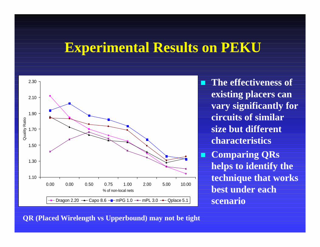
Experimental Results on PEKU

n The effectiveness of existing placers can vary significantly for circuits of similar size but different characteristics

n Comparing QRshelps to identify the technique that works best under each scenario

1.10

1.30

1.50

1.70

1.90

2.10

2.30

0.00 0.00 0.50 0.75 1.00 2.00 5.00 10.00% of non-local nets

Qua

lity

Rat

io

Dragon 2.20 Capo 8.6 mPG 1.0 mPL 3.0 Qplace 5.1

QR (Placed Wirelength vs Upperbound) may not be tight

High Interest in the Community

Timing-driven Placement Examples with Known Optimal (TPEKO)

n Obtain a placement for the circuit from any available tool

n Perform timing analysis on the circuit

n Create an artificial combinational path with equal or larger delay than the longest path

n Guarantee the cells in the path are adjacent to each other

n Make necessary modifications

Original longest path

Artificial path

Evaluating Timing-Driven Placement Algorithms Using TPEKO

n Evaluating two state-of-the-art FPGA placement algorithmsuVPR [Marquardt et al.

2000]u PATH [Kong 2002]

n Can be far away from the optimal for difficult examplesu 35% on averageu 54% in the worst case

1.00

1.05

1.10

1.15

1.20

1.25

1.30

1.35

1.40

1 2 3 4 5#longest path

Qu

ali

ty R

ati

o

VPR PATH

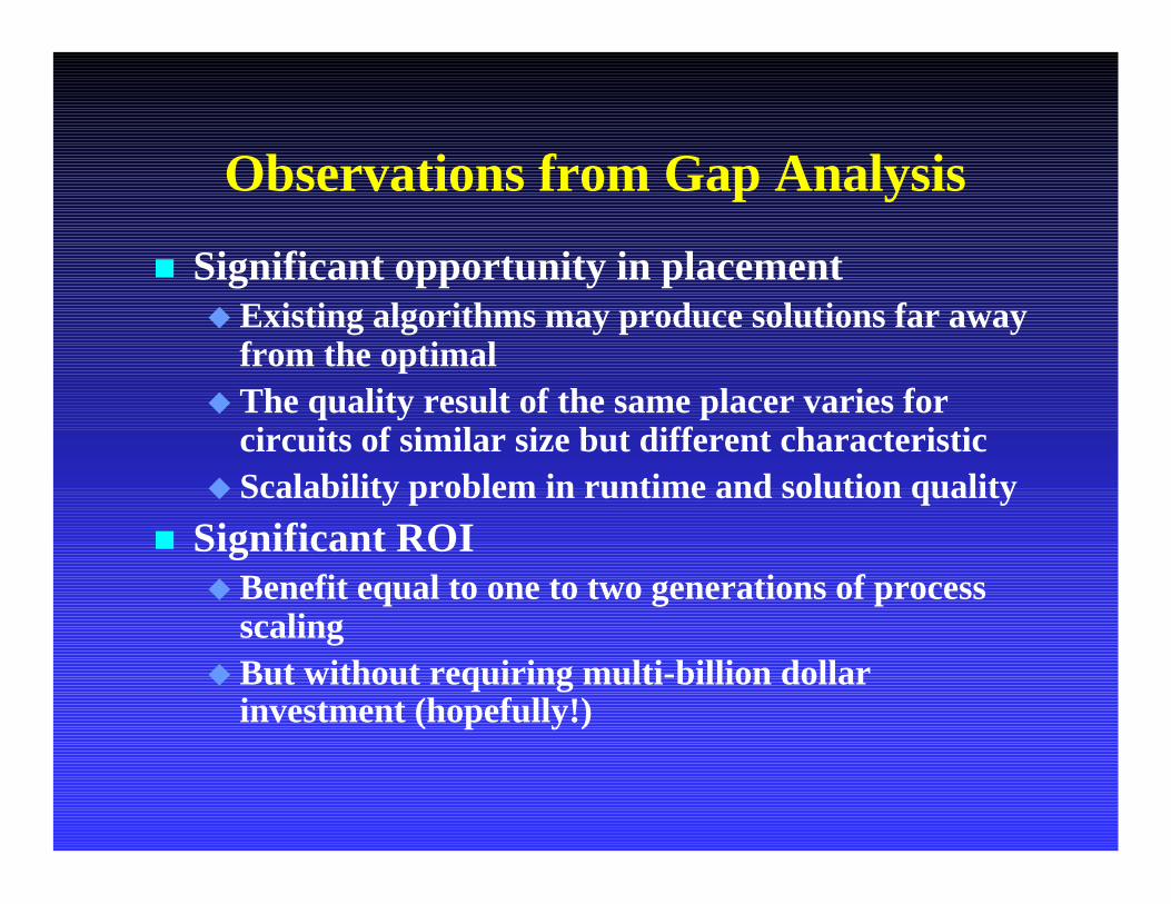
Observations from Gap Analysis

n Significant opportunity in placementuExisting algorithms may produce solutions far away

from the optimal uThe quality result of the same placer varies for

circuits of similar size but different characteristicu Scalability problem in runtime and solution quality

n Significant ROIuBenefit equal to one to two generations of process

scaling uBut without requiring multi-billion dollar

investment (hopefully!)

Outline

nn IntroductionIntroductionnn Gap Analysis of Existing Placement AlgorithmsGap Analysis of Existing Placement Algorithmsnn Scalable ParadigmScalable Paradigmnn Timing OptimizationTiming Optimizationnn RoutabilityRoutability OptimizationOptimizationnn ConcludingConcluding RemarksRemarksnn ApplicationApplicationuuMultiMulti--Million Gate FPGA PlacementMillion Gate FPGA Placement

Scalable Paradigms for Placement

n Assertion: some form of hierarchy is essentialn Three main paradigms:

1) Top-downF Generalized recursive partitioning defines the hierarchy

2) Bottom-up (multilevel)F Generalized recursive clustering defines the hierarchy

3) FlatF Flat on the outside, but hierarchical internally

n Caveatsu Scalable may be slower than O(N), due to Moore’s lawu Focus on global placement; assume scalability of

legalization and detailed placement

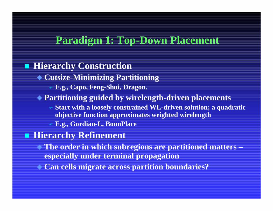
Paradigm 1: Top-Down Placement

n Hierarchy ConstructionuCutsize-Minimizing Partitioning

F E.g., Capo, Feng-Shui, Dragon.

u Partitioning guided by wirelength-driven placements F Start with a loosely constrained WL-driven solution; a quadratic

objective function approximates weighted wirelengthF E.g., Gordian-L, BonnPlace

n Hierarchy RefinementuThe order in which subregions are partitioned matters –

especially under terminal propagationuCan cells migrate across partition boundaries?

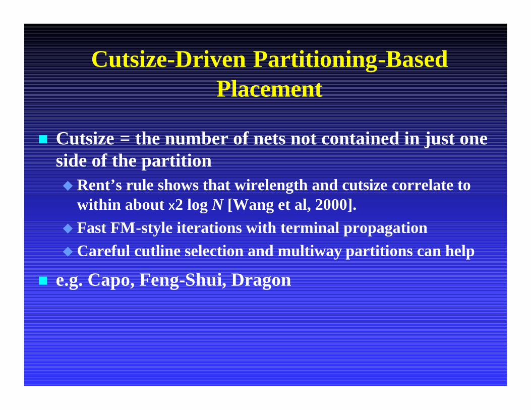
Cutsize-Driven Partitioning-Based Placement

n Cutsize = the number of nets not contained in just one side of the partitionuRent’s rule shows that wirelength and cutsize correlate to

within about X2 log N [Wang et al, 2000].u Fast FM-style iterations with terminal propagationuCareful cutline selection and multiway partitions can help

n e.g. Capo, Feng-Shui, Dragon

Initially, there is only netlist connectivity; no spatial information is available.

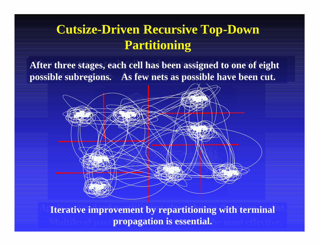
Cutsize-Driven Recursive Top-Down Partitioning

Apply a standard partitioning algorithm to the given netlist.Multilevel partitioning algorithms are the most effective.

After two stages, each cell has been assigned to one of four possible subregions. As few nets as possible have been cut.After three stages, each cell has been assigned to one of eight possible subregions. As few nets as possible have been cut.

Iterative improvement by repartitioning with terminal propagation is essential.

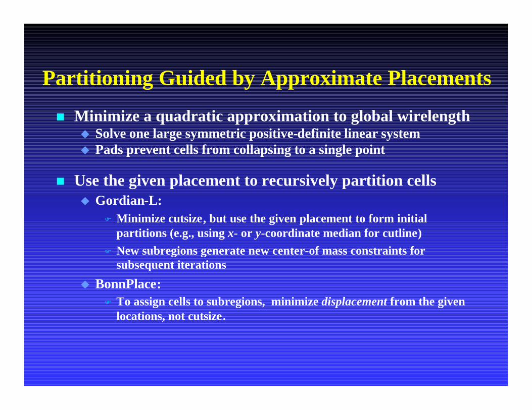
Partitioning Guided by Approximate Placements

n Minimize a quadratic approximation to global wirelengthu Solve one large symmetric positive-definite linear systemu Pads prevent cells from collapsing to a single point

n Use the given placement to recursively partition cellsu Gordian-L:

F Minimize cutsize, but use the given placement to form initial partitions (e.g., using x- or y-coordinate median for cutline)

F New subregions generate new center-of mass constraints for subsequent iterations

u BonnPlace: F To assign cells to subregions, minimize displacement from the given

locations, not cutsize.

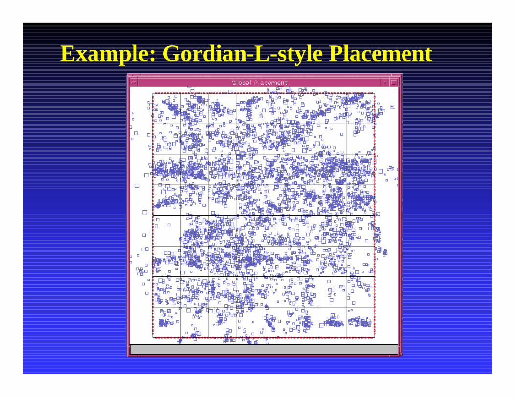
Example: Gordian-L-style Placement

Hierarchy Adjustments in Top-Down Placement by Iterative Refinement

n K-way partitioning followed by localized repartitioning with terminal propagation (Feng-Shui).

n Initial cutsize-driven quadrisection followed by bin swapping, each bin being a block of the partition, with wirelength-based annealing only at the finest level (Dragon).

n Unconstrained quadratic wirelength minimization over 2x2 windows of overlapping subregions, followed by repartioning inside each window (BonnPlace).

Paradigm 2: Multilevel Placement

n Coarsening: build the hierarchy by recursive aggregation (generalized clustering)

n Relaxation: improve the placement at each level by localized optimization

n Interpolation: transfer coarse-level solution to adjacent, finer level (generalized declustering)

n Multilevel Flow: multiple traversals over multiple hierarchies (V-cycle variations)

Multi-Level Optimization Framework

Interpolation &Relaxation (optimization)

Coarsening(Clustering)

Pro

blem

siz

e de

crea

ses

•Multilevel coarsening generates smaller problem sizes at coarser levels àfaster optimization at coarser levels

•May explore different aspects of the solution space at different levels•Gradual refinement on good solutions from coarser levels is very efficient•Successful in many applications

•Originally developed for PDEs•Recent success in VLSI CAD: partitioning, placement, routing

Given problem

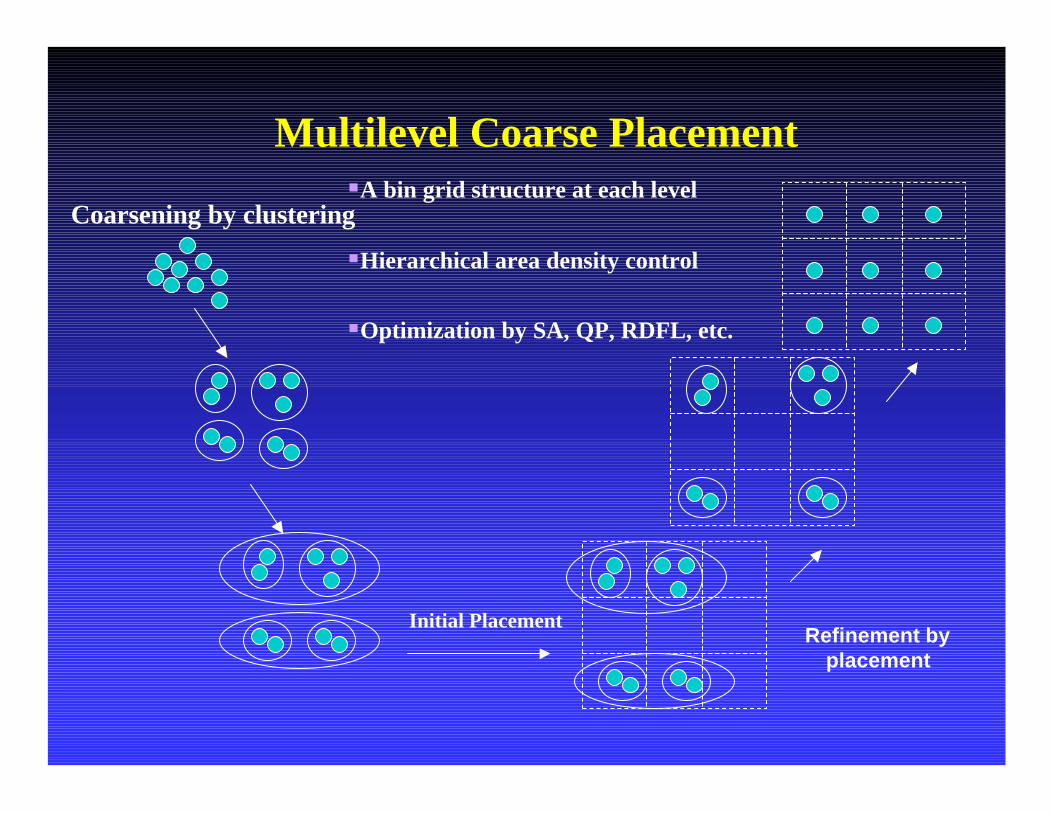
Multilevel Coarse Placement

Coarsening by clustering

Refinement by placement

Initial Placement

§A bin grid structure at each level

§Hierarchical area density control

§Optimization by SA, QP, RDFL, etc.

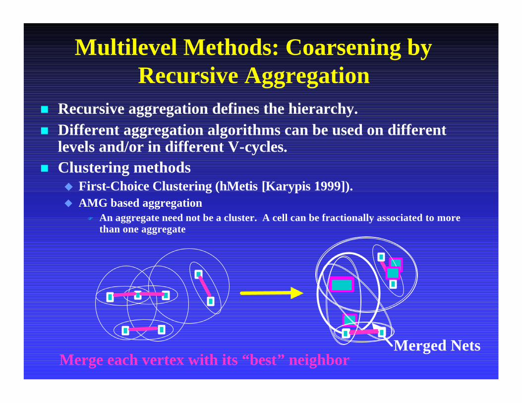
Multilevel Methods: Coarsening by Recursive Aggregation

n Recursive aggregation defines the hierarchy.n Different aggregation algorithms can be used on different

levels and/or in different V-cycles.n Clustering methods

u First-Choice Clustering (hMetis [Karypis 1999]).u AMG based aggregation

F An aggregate need not be a cluster. A cell can be fractionally associated to more than one aggregate

Merge each vertex with its “best”neighborMerged Nets

Multilevel Methods: Relaxation(Intralevel Optimization)

n Iterative improvement at each level by fast, localized computationuDiscrete permutation enumerations; swappinguUnconstrained quadratic wirelength minimization on

subsets uNetwork-flow based improvement on subsets (RDFL)

n Local relaxation is sufficient. Global improvement comes from the multilevel hierarchy.

n Relaxations at finer levels may be quite different, e.g., more discrete, than relaxations at coarser levels.

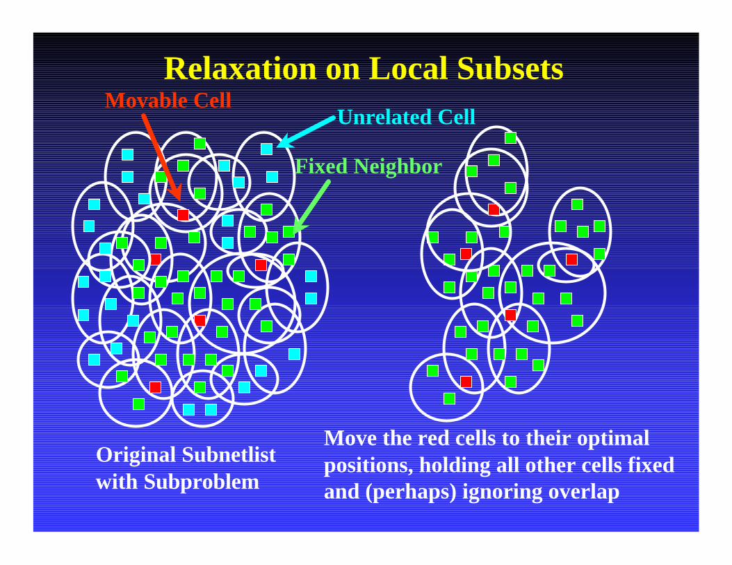
Relaxation on Local Subsets

Original Subnetlistwith Subproblem

Move the red cells to their optimal positions, holding all other cells fixed and (perhaps) ignoring overlap

Unrelated Cell

Fixed Neighbor

Movable Cell

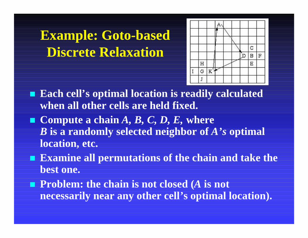
Example: Goto-based Discrete Relaxation

n Each cell’s optimal location is readily calculated when all other cells are held fixed.

n Compute a chain A, B, C, D, E, whereB is a randomly selected neighbor of A’s optimal location, etc.

n Examine all permutations of the chain and take the best one.

n Problem: the chain is not closed (A is not necessarily near any other cell’s optimal location).

Example: Quadratic Relaxation on Noncontiguous Subsets (QRS)

n Select a subset M of cells to moven Identify other cells and pads, F, connected to

M by nets in

n Decouple the horizontal and vertical problems.n M is obtained as segments of length k along a

DFS vertex traversal of the netlist

}.|{ φ≠∩∈= MeEeE M

Solving the QRS subproblem

n Problem formulation (horizontal case):

n Iteratively solve the weighted quadratic minimization problem, using the current solution to determine the weight (as in Gordian-L)

n May result in cell overlap!

number. small is , )(||

1 where

|)(|))((

min )()(

2

ε

ε

∑

∑ ∑

∈

∈ ∈

=

+−−

eve

Ee evk

ek

e

vxe

x

xvxxvx

M

Ripple-move legalization [Hur and Lillis, 2000]Because many forms of subset relaxation ignore overlap, post-relaxation cell swaps may be needed to remove overlap.

Define a DAG on neighboring bins. Edge cost reflects the best wirelength gain over all cell swaps between two bins.Calculate a max-gain monotone path on the bin-grid graph

Multilevel Methods: Interpolation(Generalized Declustering)

n Goal: transfer a partial solution from a coarser level to its adjacent finer level

n Simplest approach: place all components of a cluster at its center

n Better approach: place each component of an aggregate at the weighted average of the aggregates to which it is strongly connected.

n Optionally: impose constraints; e.g., the average location of the components can be held fixed.

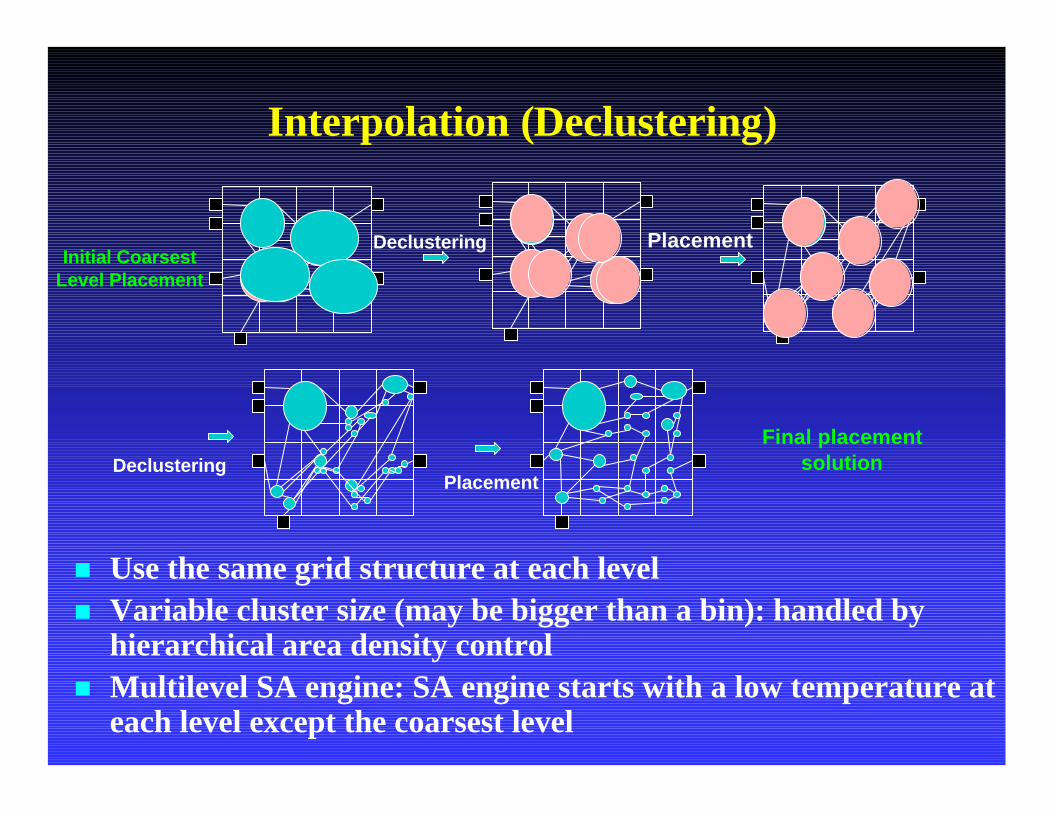
Interpolation (Declustering)

Initial Coarsest Level Placement

Declustering Placement

DeclusteringPlacement

Final placement solution

n Use the same grid structure at each leveln Variable cluster size (may be bigger than a bin): handled by

hierarchical area density controln Multilevel SA engine: SA engine starts with a low temperature at

each level except the coarsest level

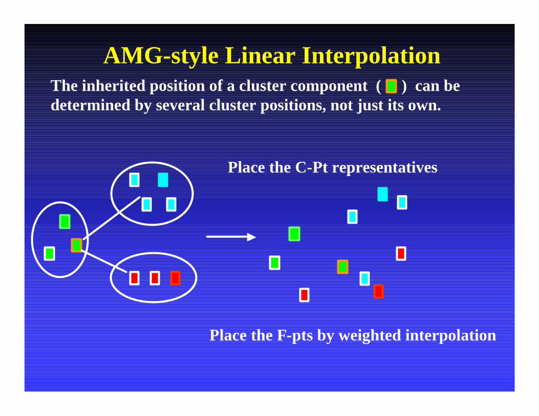
AMG-style Linear Interpolation

Place the C-Pt representatives

The inherited position of a cluster component ( ) can be determined by several cluster positions, not just its own.

Place the F-pts by weighted interpolation

AMG-based Linear Interpolation[A. Brandt 1986]

interpolation

constantAMG

jijvFjijvCi vavavjj points points −−

Σ+Σ=

clusterNext finer level cells

Within each cluster, select the one with maximum degree as C-point; others are

considered as F-points

C-point

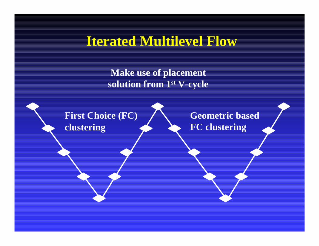
Iterated Multilevel Flow

Make use of placement solution from 1st V-cycle

First Choice (FC)clustering

Geometric basedFC clustering

Iterated Multilevel Flow

Iterated V-Cycles F-Cycle

Backtracking V-Cycle

Sample Impact of the Multilevel Components to mPL’s overall quality

n First-Choice Clustering: 3— 4% reduced WLn QRS Relaxation: 5— 6% reduced WLn AMG Interpolation: 2— 3% reduced WLn Iterated V-cycles: 2— 8% reduced WL

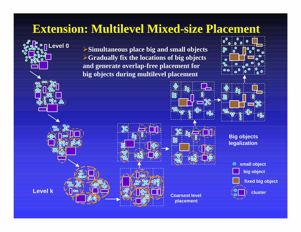
Extension: Multilevel Mixed-size Placement Level 0

Level kCoarsest level

placement

Big objects legalization

big object

small object

fixed big object

cluster

ØSimultaneous place big and small objectsØGradually fix the locations of big objects and generate overlap-free placement for big objects during multilevel placement

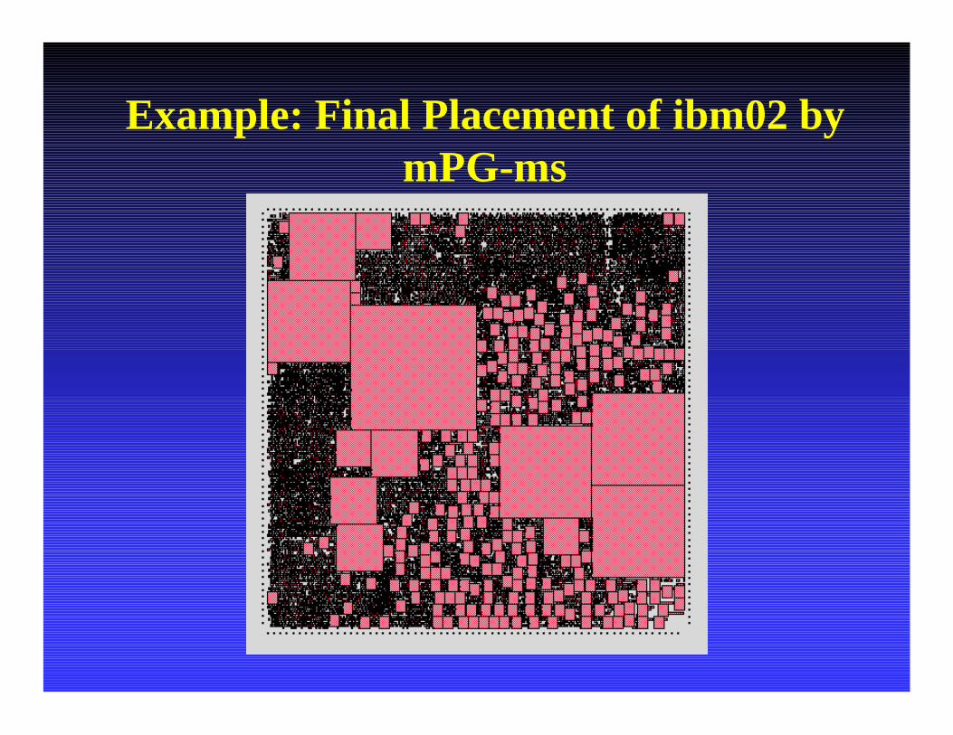
Example: Final Placement of ibm02 by mPG-ms

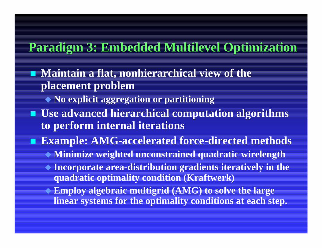
Paradigm 3: Embedded Multilevel Optimization

n Maintain a flat, nonhierarchical view of the placement problemuNo explicit aggregation or partitioning

n Use advanced hierarchical computation algorithms to perform internal iterations

n Example: AMG-accelerated force-directed methods uMinimize weighted unconstrained quadratic wirelengthu Incorporate area-distribution gradients iteratively in the

quadratic optimality condition (Kraftwerk)uEmploy algebraic multigrid (AMG) to solve the large

linear systems for the optimality conditions at each step.

Outline

nn IntroductionIntroductionnn Gap Analysis of Existing Placement AlgorithmsGap Analysis of Existing Placement Algorithmsnn Scalable ParadigmScalable Paradigmnn Timing OptimizationTiming Optimizationnn RoutabilityRoutability OptimizationOptimizationnn ConcludingConcluding RemarksRemarksnn ApplicationApplicationuu MultiMulti--Million Gate FPGA PlacementMillion Gate FPGA Placement

Timing Optimization

n Additional goal: to minimize longest-path delay or maximize the minimum slack.

n Difficulties:uExponential number of paths.uComplex timing constraints –multi-clock domain,

multi-cycle, etc.

n Existing Algorithmsu Path-based algorithmsuNet-based algorithms

Path-based Algorithms

n Directly minimize the longest path delay. n Popular approaches:uExplicitly reduce the maximum length of a set of

paths; the set could be pre-computed or dynamically adjusted.F [Burstein & Youssef, 1985, Swartz & Sechen, 1995]

a

b

cd

e

1

2

3 4

5

6

D(a)+D(c)+D(d)D(b)+D(c)+D(d)D(a)+D(c)+D(e)D(b)+D(c)+D(e)

MAX {D(i): edge delay (cell delay included)

Mathematical Programming based Approaches

n Popular approaches (cont’d):uMathematical programming by introducing

auxiliary variables (arrival time)F [Jackson & Kuh, 1989, Srinivasan et al, 1991,

Hamada et al, 1993, … ]

a

b

cd

e

1

2

3 4

5

6

A(i): arrival time at i

A(1)+D(a) ≤A(3) : edge(a)A(2)+D(b) ≤A(3) : edge(b)… …A(5) ≤T(5) : endpoint 5A(6) ≤T(6) : endpoint 6

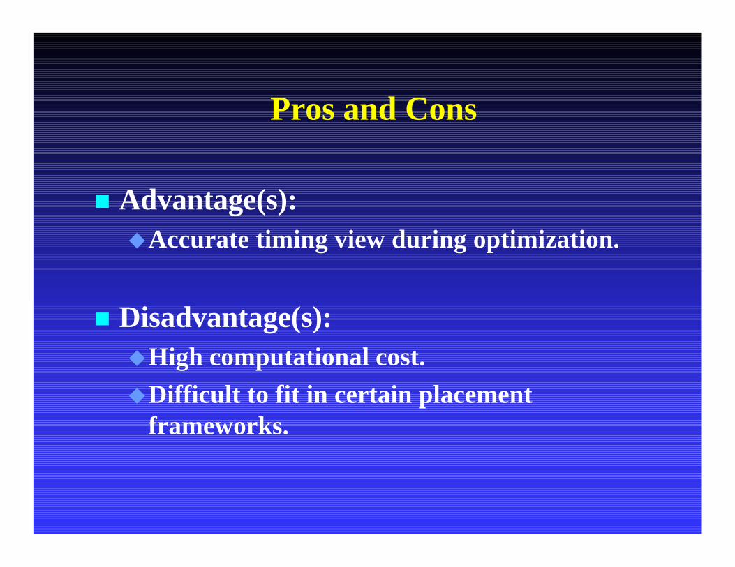
Pros and Cons

n Advantage(s):uAccurate timing view during optimization.

n Disadvantage(s):uHigh computational cost.uDifficult to fit in certain placement

frameworks.

Net-based Algorithms

n Timing constraints are translated into net weights (net-weighting) or length constraints (delay-budgeting).

n Delay budgeting: distribute slacks to all edges in the circuit to achieve zero-slack u [Hauge et al, 1987, Gao et al, 1991, Luk 1991, Youssef et al, 1992,

Tellez et al, 1996, … ]

a

b

cd

e

1

2

3 4

5

6

D(a) ≤ τ1D(b) ≤ τ2D(c) ≤ τ3D(d) ≤ τ4D(e) ≤ τ5

Timing-Driven Placement with Delay Budgeting

n Construct a placement to meet all budgets.u If all budgets are met, timing is GUARANTEED!

n Difficulty: Too many possible budgeting solutions and do not know which can be satisfied a priori.uBudgeting is often done in structural domain without

physical feasibility considerationuUnify placement and delay budgeting?

F [Sarrafzadeh et al, 1997; Halpin et al, 2001; Yang et al, 2002]

Net Weighting

n Timing criticalities are translated into net weights (soft constraints); then compute a placement which minimizes total weighted delay (or WL).

a

b

cd

e

1

2

3 4

5

6

Cost = w(a)*D(a) + w(b)*D(b) + w©*D(c) + w(d)*D(d) + w(e)*D(e)

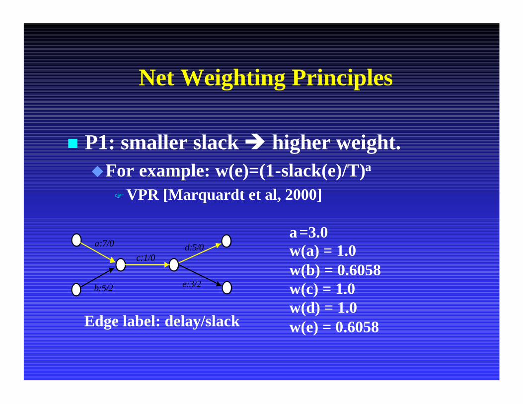
Net Weighting Principles

n P1: smaller slack è higher weight.uFor example: w(e)=(1-slack(e)/T)α

FVPR [Marquardt et al, 2000]

a:7/0

b:5/2

c:1/0d:5/0

e:3/2

α=3.0w(a) = 1.0w(b) = 0.6058w(c) = 1.0w(d) = 1.0w(e) = 0.6058Edge label: delay/slack

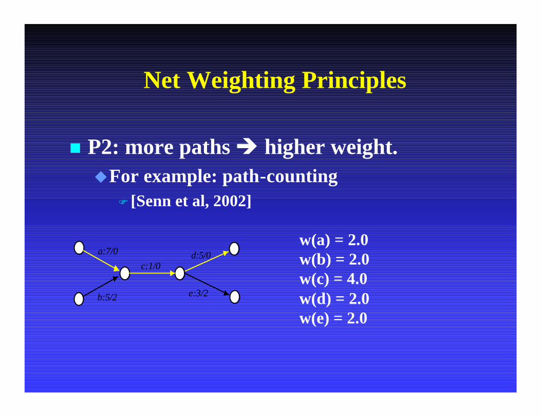
Net Weighting Principles

n P2: more paths è higher weight.uFor example: path-counting

F [Senn et al, 2002]

a:7/0

b:5/2

c:1/0d:5/0

e:3/2

w(a) = 2.0w(b) = 2.0w(c) = 4.0w(d) = 2.0w(e) = 2.0

Ideal Net Weighting

n Need to consider both principles together

a:7/0

b:5/2

c:1/0d:5/0

e:3/2

Ideally, we want

w(c) > w(a)=w(d) > w(b)=w(e)

All Path Net Weighting Problem

n Challenge: can we compute the impact of all paths through an edge, properly scaled by their slacks? u i.e., for each edge e, compute

F w(e) = Σ∀ p ∋ e f(slack(p))

a:7/0

b:5/2

c:1/0d:5/0

e:3/2

w(a)= f(slack(a-c-d)) +f(slack(a-c-e))

w(c)= f(slack(a-c-d)) +f(slack(b-c-d)) +f(slack(a-c-e)) +f(slack(b-c-e))

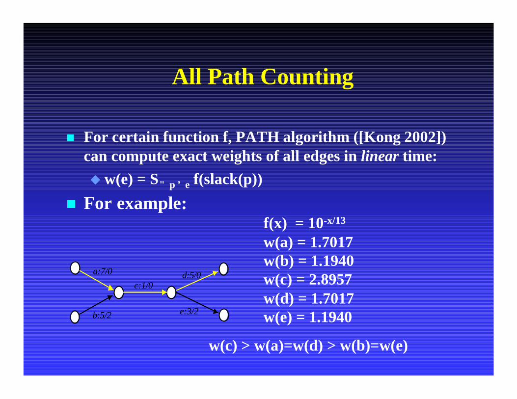
All Path Counting

n For certain function f, PATH algorithm ([Kong 2002]) can compute exact weights of all edges in linear time:uw(e) = Σ∀ p ∋ e f(slack(p))

n For example:

a:7/0

b:5/2

c:1/0d:5/0

e:3/2

f(x) = 10-x/13

w(a) = 1.7017w(b) = 1.1940w(c) = 2.8957w(d) = 1.7017w(e) = 1.1940

w(c) > w(a)=w(d) > w(b)=w(e)

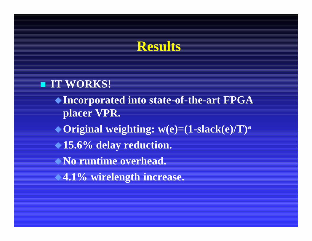
Results

n IT WORKS!uIncorporated into state-of-the-art FPGA

placer VPR.uOriginal weighting: w(e)=(1-slack(e)/T)α

u15.6% delay reduction.uNo runtime overhead.u4.1% wirelength increase.

Outline

nn IntroductionIntroductionnn Gap Analysis of Existing Placement AlgorithmsGap Analysis of Existing Placement Algorithmsnn Scalable ParadigmScalable Paradigmnn Timing OptimizationTiming Optimizationnn RoutabilityRoutability OptimizationOptimizationnn Concluding RemarksConcluding Remarksnn ApplicationApplicationuuMultiMulti--Million Gate FPGA PlacementMillion Gate FPGA Placement

Routability Optimization

n Aggressive WL minimization != routabilityn Routability-driven placementuRoutability modelinguSolution techniques for routability control

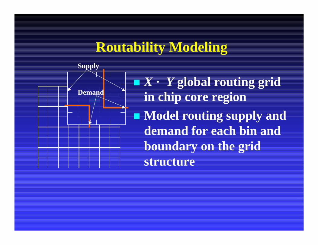
Routability Modeling

n X × Y global routing grid in chip core region

n Model routing supply and demand for each bin and boundary on the grid structure

Supply

Demand

Categories of Routability Modelinig

n Topology-free modelinguNo routing topology generateduFast

n Topology-based modelinguSteiner tree topology generationuProvide upper bound for routability

estimationuHigh complexity

Topology-free Modeling

n Bounding-box (BBOX)-based modeling [Cheng 1994]

n Probabilistic analysis-based modeling [Lou et al, 2001]

n Rent’s rule-based modeling [Yang et al, 2002]n Pin density-based modeling [Hu & Marek-

Sadowska 2002, Brenner & Rohe, 2003]

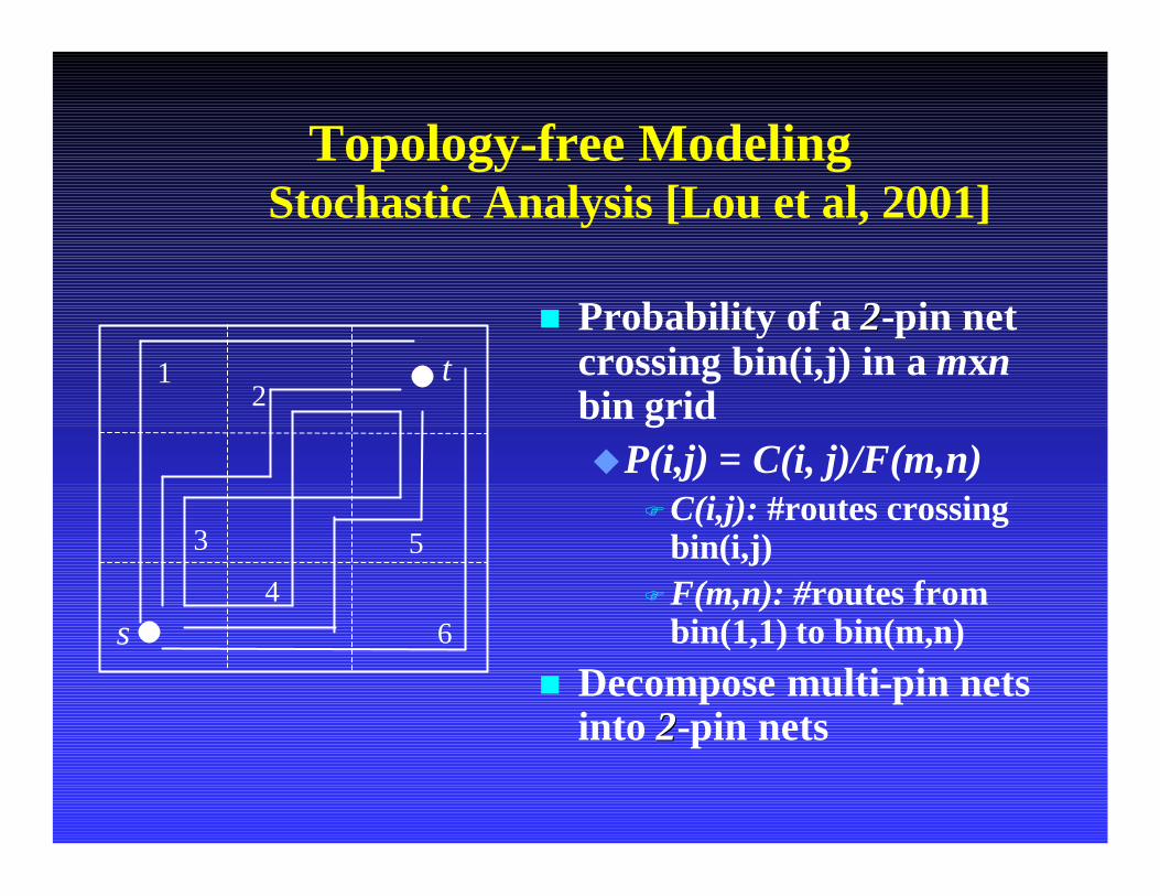
Topology-free Modeling Stochastic Analysis [Lou et al, 2001]

n Probability of a 22-pin net crossing bin(i,j) in a mxn bin griduP(i,j) = C(i, j)/F(m,n)

FC(i,j): #routes crossing bin(i,j)

FF(m,n): #routes frombin(1,1) to bin(m,n)

n Decompose multi-pin nets into 22-pin nets

12

3

4

5

6s

t

Topology-free ModelingPin Density Based

[Hu & Marek-Sadowska 2002,Brenner & Rohe, 2003]

n Calculated weighted wirelength

u Di: degree of net iu BBi : bounding box of net iu Ps(b) : heuristic function

capturing pin density in bin bn Can be combine with

probabilistic analysis-based modeling

ii i

ibs

i BBD

bPwCF ∑

∑

= ∈

)(

F’= (1+1+1)/3*4=4

Let P(b) linear with respect to #pin

Topology-based Modeling

n Precomputed Steiner tree topology for wiring demand estimation [Mayrhofer & Lauther, 1990]

n Congestion-avoidance two-bend routing for 2-pin nets [Chang et al, 2003]

n IncAtree with incremental updates support for multi-pin nets [Chang et al, 2003]

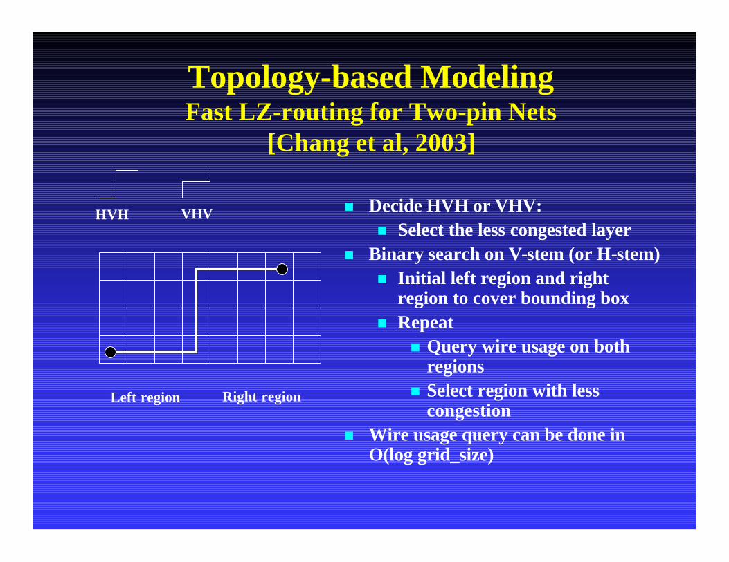
Topology-based ModelingFast LZ-routing for Two-pin Nets

[Chang et al, 2003]

n Decide HVH or VHV:n Select the less congested layer

n Binary search on V-stem (or H-stem)n Initial left region and right

region to cover bounding boxn Repeat

n Query wire usage on both regions

n Select region with less congestion

n Wire usage query can be done in O(log grid_size)

Left region Right region

HVH VHV

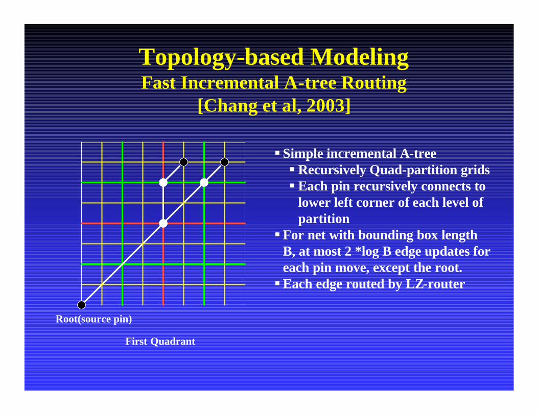
Topology-based ModelingFast Incremental A-tree Routing

[Chang et al, 2003]

§ Simple incremental A-tree§Recursively Quad-partition grids§ Each pin recursively connects to

lower left corner of each level of partition

§For net with bounding box length B, at most 2 *log B edge updates for each pin move, except the root. §Each edge routed by LZ-router

First Quadrant

Root(source pin)

Optimization Techniques for Routability

n Net weightingu Transfer congestion picture into bin weights and optimization

weighted WL u Used in iterative placement, such as SA-based placer [Hu &

Marek-Sadowska, 2002, Chang et al, 2003]

n Cell weighting (a.k.a cell inflation)u Weight cell size based on the congestion picture u Use partitioner or implicit/explicit bin density control to move

inflated cell out of congested region u Used in constructive placement and iterative

placement[Parakh 1998, Brenner & Rohe, 2003, Yang et al, 2003]

Outline

nn IntroductionIntroductionnn Gap Analysis of Existing Placement AlgorithmsGap Analysis of Existing Placement Algorithmsnn Scalable ParadigmScalable Paradigmnn Timing OptimizationTiming Optimizationnn RoutabilityRoutability OptimizationOptimizationn Concluding Remarksnn ApplicationApplicationuuMultiMulti--Million Gate FPGA PlacementMillion Gate FPGA Placement

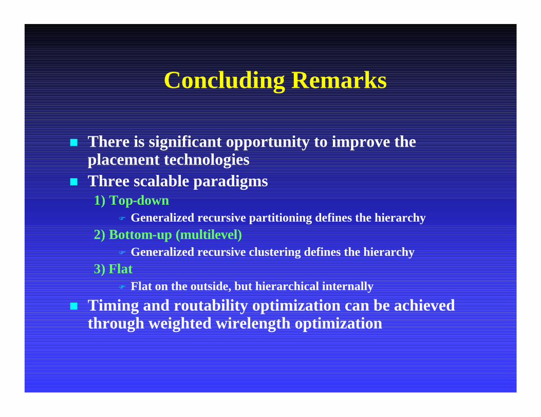
Concluding Remarks

n There is significant opportunity to improve the placement technologies

n Three scalable paradigms1) Top-down

F Generalized recursive partitioning defines the hierarchy2) Bottom-up (multilevel)

F Generalized recursive clustering defines the hierarchy3) Flat

F Flat on the outside, but hierarchical internally

n Timing and routability optimization can be achieved through weighted wirelength optimization

Outline

nn IntroductionIntroductionnn Gap Analysis of Existing Placement AlgorithmsGap Analysis of Existing Placement Algorithmsnn Scalable ParadigmScalable Paradigmnn Timing OptimizationTiming Optimizationnn RoutabilityRoutability OptimizationOptimizationnn Concluding RemarksConcluding Remarksn ApplicationuMulti-Million Gate FPGA Placement

Large Scale Circuit Placement: Gap and Promise -...

Documents

Transcript of Large Scale Circuit Placement: Gap and Promise -...