Large Investors, Price Manipulation, and Limits to...
49
Review of Finance (2006) 10: 643–691 © Springer 2006 Large Investors, Price Manipulation, and Limits to Arbitrage: An Anatomy of Market Corners FRANKLIN ALLEN 1 , LUBOMIR LITOV 2 and JIANPING MEI 3 1 The Wharton School, University of Pennsylvania; 2 Olin School of Business, Washington University in St. Louis; 3 Leonard Stern School of Business, New York University, and Cheung Kong Graduate School of Business Abstract. Corners were prevalent in the nineteenth and early twentieth century. We first develop a rational expectations model of corners and show that they can arise as the result of rational behavior. Then, using a novel hand-collected data set, we investigate price and trading behavior around several well-known stock market and commodity corners which occurred between 1863 and 1980. We find strong evidence that large investors and corporate insiders possess market power that allows them to manipulate prices. Manipulation leading to a market corner tends to increase market volatility and has an adverse price impact on other assets. We also find that the presence of large investors makes it risky for would-be short sellers to trade against the mispricing. Therefore, regulators and exchanges need to be concerned about ensuring that corners do not take place since they are accompanied by severe price distortions. 1. Introduction Although stock markets are far better regulated today than in the nineteenth cen- tury, market manipulations by large investors and insiders still occur around the world. Most recently, in August 2004, Citigroup placed sell orders for no fewer than 200 different types of Eurozone government bonds worth almost 12.9 billion in the space of 18 seconds. They bought back at lower prices the same morning and earned profits of 18.2 million. 1 This action reduced the subsequent liquidity of the market significantly. In May 1991, a bond trader at Salomon Brothers was discovered attempting to corner the market in two-year U.S. Treasury notes. 2 Dur- ing the 1990s bull market, numerous price manipulation schemes for penny stocks For valuable comments, we are grateful to an anonymous referee, Niall Ferguson, William Goetzmann, Colin Mayer (the Editor), Gideon Saar, Chester Spatt, Richard Sylla, Jeffrey Wurgler, the conference participants at the CEPR Conference on Early Securities Markets at the Humboldt Uni- versity on October 15–16, 2004, the participants at the 2005 Western Finance Association meeting, and seminar participants at the Commodity Futures Trading Commission. 1 See the Financial Times, August 23, 2006, “The day Dr Evil wounded a financial giant”. 2 See Jegadeesh (1993) and Jordan and Jordan (1996) for detailed studies on the Treasury auction bids and the Salomon price squeeze. DOI 10.1007/s10679-006-9008-5 10:645–693
Transcript of Large Investors, Price Manipulation, and Limits to...

Review of Finance (2006) 10: 643–691 © Springer 2006
Large Investors, Price Manipulation, and Limits toArbitrage: An Anatomy of Market Corners �
FRANKLIN ALLEN1, LUBOMIR LITOV2 and JIANPING MEI3
1The Wharton School, University of Pennsylvania; 2Olin School of Business, Washington Universityin St. Louis; 3Leonard Stern School of Business, New York University, and Cheung Kong GraduateSchool of Business
Abstract. Corners were prevalent in the nineteenth and early twentieth century. We first develop arational expectations model of corners and show that they can arise as the result of rational behavior.Then, using a novel hand-collected data set, we investigate price and trading behavior around severalwell-known stock market and commodity corners which occurred between 1863 and 1980. We findstrong evidence that large investors and corporate insiders possess market power that allows them tomanipulate prices. Manipulation leading to a market corner tends to increase market volatility andhas an adverse price impact on other assets. We also find that the presence of large investors makes itrisky for would-be short sellers to trade against the mispricing. Therefore, regulators and exchangesneed to be concerned about ensuring that corners do not take place since they are accompanied bysevere price distortions.
1. Introduction
Although stock markets are far better regulated today than in the nineteenth cen-tury, market manipulations by large investors and insiders still occur around theworld. Most recently, in August 2004, Citigroup placed sell orders for no fewerthan 200 different types of Eurozone government bonds worth almost 12.9 billionin the space of 18 seconds. They bought back at lower prices the same morningand earned profits of 18.2 million.1 This action reduced the subsequent liquidityof the market significantly. In May 1991, a bond trader at Salomon Brothers wasdiscovered attempting to corner the market in two-year U.S. Treasury notes.2 Dur-ing the 1990s bull market, numerous price manipulation schemes for penny stocks
� For valuable comments, we are grateful to an anonymous referee, Niall Ferguson, WilliamGoetzmann, Colin Mayer (the Editor), Gideon Saar, Chester Spatt, Richard Sylla, Jeffrey Wurgler, theconference participants at the CEPR Conference on Early Securities Markets at the Humboldt Uni-versity on October 15–16, 2004, the participants at the 2005 Western Finance Association meeting,and seminar participants at the Commodity Futures Trading Commission.
1 See the Financial Times, August 23, 2006, “The day Dr Evil wounded a financial giant”.2 See Jegadeesh (1993) and Jordan and Jordan (1996) for detailed studies on the Treasury auction
bids and the Salomon price squeeze.
DOI 10.1007/s10679-006-9008-510:645–693
644 FRANKLIN ALLEN ET AL.
were discovered by the SEC.3 Manipulation knows no international borders. In2002, China’s worst stock-market crime was a scheme to manipulate the shareprice of a firm called China Venture Capital. Seven people, including two of thefirm’s former executives, were accused of using $700 million and 1,500 brokerageaccounts nationwide to manipulate the company share price. Krugman (1996) alsoreported a price manipulation in the copper market by a rogue trader at the Japanesetrading firm Sumitomo. More recently British Petroleum has been investigated bythe SEC for the possibility of cornering the U.S. propane market in early 2004.4
There is a growing theoretical literature on market manipulation. Hart (1977),Hart and Kreps (1986), Vila (1987, 1989), Allen and Gale (1992), Allen andGorton (1992), Benabou and Laroque (1992), and Jarrow (1992, 1994) wereamong the first to study market manipulation. Cherian and Jarrow (1995) sur-vey this early literature. Subsequent contributions include Bagnoli and Lipman(1996), Chakraborty and Yilmaz (2004a, b), and Goldstein and Guembel (2003).Kumar and Seppi (1992) discuss the possibility of futures manipulation withcash settlement. Pirrong (1993) shows how squeezes hinder price discovery andcreate deadweight losses. Vitale (2000) considers manipulation in foreign ex-change markets. Van Bommel (2003) shows the role of rumors in facilitating pricemanipulation.
In contrast, the empirical literature is quite limited. Although the wide-spreadmanipulation through stock pools before the Crash of 1929 is vividly documentedin Galbraith (1972), Mahoney (1999) and Jiang et al. (2005) find little evidenceof price manipulation for the stock pools. However, there are a few recent stud-ies that have found evidence of market manipulation. Aggarwal and Wu (2006)present a theory and some empirical evidence on stock price manipulation in theUnited States. Extending the framework of Allen and Gale (1992), they show thatmore information seekers imply greater competition for shares in a market withmanipulators, making it easier for a manipulator to enter the market and poten-tially worsen market efficiency. Using a unique dataset from SEC actions in casesof stock manipulation, they find that more illiquid stocks are more likely to bemanipulated and manipulation increases stock volatility. Khwaja and Mian (2005)discover evidence of broker price manipulation by using a unique daily trade leveldata set from the main stock market in Pakistan. They find that brokers earn at least8% higher returns on their own trades. While neither market timing nor liquidityprovision offer sufficient explanations for this result, they find compelling evidencefor a specific trade-based “pump-and-dump” price manipulation scheme. Merrick
3 For example, the SEC intervened in 1996 when the share price of Comparator Systems Corpora-tion (a finger print identification company with net assets of less than $2 million) soared from 3 centsto $1.03, valuing the company at a market capitalization of over a billion dollars. An astonishing 180million Comparator shares were traded on the Nasdaq Exchange on May 6, 1996. See also Aggarwaland Wu (2006).
4 See the Wall Street Journal of June 29, 2006, “U.S. Accuses BP of manipulating Price ofPropane”.
646
LARGE INVESTORS, PRICE MANIPULATION, AND LIMITS TO ARBITRAGE 645
et al. (2005) provide empirical evidence on learning in the market place and on thestrategic behavior of market participants by studying an attempted delivery squeezein the March 1998 long-term UK government bond futures contract traded on theLondon International Financial Futures and Options Exchange (LIFFE). Felixonand Pelli (1999) test for closing price manipulation in the Finnish stock marketand find evidence of it. They find that block trades and spread trades explained apart, but not all of the observed manipulation. Mei, Wu and Zhou (2004) constructa theoretical example in which smart money strategically takes advantage of in-vestors’ behavioral biases and manipulates the price process to make a profit. Asan empirical test, the paper presents some empirical evidence from the U.S. SECprosecution of “pump-and-dump” manipulation cases. The findings from thesecases are consistent with their model.
This paper fills a gap in the manipulation literature by studying corners. Wefirst develop a rational expectations model of the phenomenon similar to that inGrossman and Stiglitz (1980). There are two assets; one is safe and one is risky witha random payoff and an unobservable random aggregate per capita supply. Thereare three groups: arbitrageurs, the uninformed, and a manipulator. The arbitrageursreceive a signal that indicates whether the payoff on the risky asset will be highor low. We first consider equilibrium when there is no manipulator present. Thereexists a pooling equilibrium where the arbitrageurs go long in the risky asset whenthey receive a good signal and short when they receive a bad signal. The priceof the risky asset is such that the uninformed cannot distinguish between situationswhere there is a good signal and the supply is large and situations where there is badsignal and supply is low. This allows the market to clear at the same price in bothsituations. We then introduce the manipulator. He can with some probability buy upthe floating supply and this allows him to corner the market when the arbitrageursare short. They are forced to settle at a high price when the corner succeeds. Thispossibility means that they will only short the stock when the potential profits offsetthe risk of being cornered. However, for prices close to their expectation of thestock’s payoff it is not worthwhile for them to take a short position. As a resultthe market is less efficient than when corners are not possible. Nevertheless it isrational for all agents to participate.
We then go on to provide a clinical study of market corners from the robber-baron era to the Great Depression of the 1930s to the 1980s.5 This involves severalcontributions: first, we have put together by hand a novel data set of price andtrading volume based on historical newspapers from the New York Times and theWall Street Journal from 1863–1980. This allows us to provide the first system-atic account of some well-known market corners in US financial history. Second,we present some unique evidence on the price and volume patterns of successfulcorners. We show that market corners tend to increase market volatility and havean adverse price impact on other assets. Third, we demonstrate that the presence of
5 Jarrow (1992) provides a collection of early references on attempted corners in individualcommon stocks.
647
646 FRANKLIN ALLEN ET AL.
large investors makes it extremely risky for short sellers to trade against mispricingin the stock market. This creates severe limits to arbitrage in the stock market thatimpede market efficiency. Therefore, regulators and exchanges need to ensure thatcorners do not take place since they are accompanied by severe price distortions.
The structure of the paper is as follows. Section 2 presents a simple modelof market corners. Section 3 considers the data and institutional background. Theempirical results are presented in Section 4. Section 5 contains concluding remarks.
2. Theoretical Analysis
2.1. THE MODEL
The model of corners developed in this section is a variant of Grossman andStiglitz’s (1980) rational expectations model. The model shows how cornerscan occur when everybody is behaving rationally. As is standard in rationalexpectations models, all agents know the structure and parameters of the model.
Assets
There are two assets, which are traded in competitive markets at date 0. The firstis a storage technology and yields 1 at date 1 for every 1 invested at date 0. Thesecond is risky. It is traded at price P at date 0 and has a random payoff v at date 1that is observable where
v = θ + ε. (1)
θ and ε are independent random variables that cannot be publicly observed. As wewill see, some traders can privately observe θ . The distribution of θ is
θB = Eθ − η with probability 0.5,θG = Eθ + η with probability 0.5.
(2)
The mean of the distribution is Eθ and the variance is η2. θB corresponds to the badstate and θG to the good one. ε is normally distributed with mean 0 and varianceσ 2
ε . Since θ and ε are independently distributed we have
σ 2v = η2 + σ 2
ε . (3)
The aggregate per capita supply of the risky asset at date 0, x, that is availablefor trading is stochastic. This is the “free float”. It is uniformly distributed between0 and xH , is independent of θ and ε, and cannot be observed.
648

LARGE INVESTORS, PRICE MANIPULATION, AND LIMITS TO ARBITRAGE 647
Agents
There are three types of agent, the uninformed, the arbitrageurs, and the manipu-lator.
The uninformed constitute a proportion λ of the population, and they behavecompetitively. They have a constant absolute risk aversion (CARA) utility function,
U(W1) = −exp[−γ W1], (4)
where W1 is wealth at date 1. Each uninformed person is endowed with wealthW0 at date 0 and purchases SU of the safe asset and XU of the risky asset so theirbudget constraints at dates 0 and 1 are
W0 = SU + PXU, (5)
W1 = SU + vXU. (6)
The second type of agent is the arbitrageurs. They are risk neutral, behave com-petitively, and are a proportion 1 − λ of the population. The amount they can tradeis constrained by their wealth. The largest long position they can each take is +X∗
A
and the largest short position is −X∗A. This is the restriction that limits arbitrage.
The third type of agent is the manipulator. He is also risk neutral. He is anegligible proportion of the population but has significant wealth. He behavesstrategically rather than competitively. His demand for the risky asset is XM . Forthe first part of the analysis we exclude the manipulator and consider only theuninformed and the arbitrageurs.
2.2. EQUILIBRIUM WITH EVERYBODY UNINFORMED
We start by considering the case where neither the uninformed nor the arbitrageurscan observe θ . This will act as a benchmark for the case where only the arbitrageurscan observe θ . The sequence of events in this case is as follows. At date 0, theuninformed and arbitrageurs submit their demand functions and the market for therisky asset clears at price P . At date 1 the risky asset pays off v.
It can be shown using the moment generating function for the normal distribu-tion that the demand of the uninformed XU is given implicitly by
(Eθ − P − γ XUσ 2ε )(1 + e2γ ηXu) + η(1 − e2γ ηXu) = 0. (7)
If the arbitrageurs are uninformed their demand will be as follows
XA = −X∗A for P > Eθ,
= −X∗A to + X∗
A for P = Eθ,
= +X∗A for P < Eθ. (8)
649

648 FRANKLIN ALLEN ET AL.
Figure 1. Possible equilibria when everybody is uninformed.
Market clearing requires
λXU + (1 − λ)XA = x. (9)
The form of the equilibrium depends on how large a position the arbitrageurscan take relative to the aggregate per capita supply. Suppose initially that X∗
A =X∗
A1 where
(1 − λ)X∗A1 ≥ xH . (10)
In this case the equilibrium has the form shown by the solid line in Figure 1. Thearbitrageurs bid the price to P = Eθ and the uninformed hold nothing at this pricesince they are risk averse so XA = x/(1 − λ) ≤ X∗
A1.In the case X∗
A = X∗A2 where
(1 − λ)X∗A2 < xH , (11)
the arbitrageurs do not have enough wealth to hold the entire supply when x ishigh. In this case the price must fall so that the uninformed will be willing to holdthe asset. Since P < Eθ the arbitrageurs will have XA = X∗
A2. Using this with (7)in (9) and rearranging gives
P = Eθ − γ XUσ 2ε + η
(1 − e2γ ηXU
1 + e2γ ηXU
)where XU = x − (1 − γ )X∗
A2
λ. (12)
650

LARGE INVESTORS, PRICE MANIPULATION, AND LIMITS TO ARBITRAGE 649
Figure 2. Possible fully revealing equilibria.
The equilibrium is shown in Figure 1. For x ≤ (1 − λ)X∗A2, only the arbitrageurs
hold the asset and then for higher x the relationship between P and x is given by(12) as shown by the dotted line.
2.3. EQUILIBRIUM WITH JUST ARBITRAGEURS INFORMED
Suppose next that only the arbitrageurs observe θ at date 0 before they trade. Ifthey observe θG(θB), we say that they receive good (bad) news. There are againa number of forms the equilibrium can take. Suppose (10) is satisfied. Similarlyto Figure 1, the arbitrageurs bid the price to reflect the information they receiveand hold all of the assets. The equilibrium price is fully revealing as shown inFigure 2 by the solid lines. When good news is observed the price is bid to θG andthe uninformed know that v is normally distributed with mean θ and variance σ 2
ε
When bad news is received the price is bid to θB and the uninformed again know v
is normally distributed but now with mean θB .When (11) is satisfied then the uninformed must again hold some of the asset.
One possibility is that prices are fully revealing. Figure 2 shows this type of equi-librium. When the arbitrageurs observe the good signal, they hold all of the riskyassets for x ≤ (1 − λ)X∗
A2 at P = θG. For x > (1 − λ)X∗A2, the uninformed hold
the remainder of the risky assets. Since they are able to deduce the arbitrageurs’information from the price we have using the fact that v is N(θG, σ 2
ε ) and themoment generating function for the normal distribution,
XU = θG − P
γ σ 2ε
. (13)
651

650 FRANKLIN ALLEN ET AL.
Using this and XA = X∗A2 in the market-clearing condition (9), we obtain similarly
to (12) that the demand curve is given by
P = θG + γ σ 2ε
λ[(1 − λ)X∗
A2 − x]. (14)
When bad news is received the analysis is the same except that θG is replaced by θB .The equilibrium in Figure 2 is special in that it arises because of the discretenessof the signals received by the arbitrageurs. If θG and θB are close together and theuninformed hold the asset, then prices can not fully reveal the information of thearbitrageurs and a partial pooling equilibrium will exist.
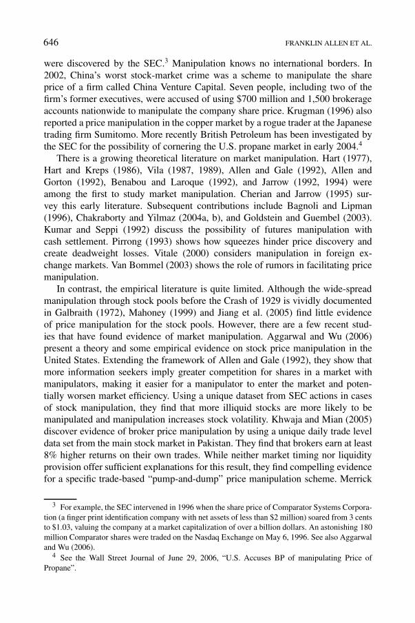
An example of such a partial pooling equilibrium is shown in Figure 3. For therange of prices P1 > P > P2 marked “Pooling”, the uninformed cannot distinguishbetween good news and a high value of x and bad news and a low value of x.Since good news and bad news are equally likely and x is uniformly distributed,no information is contained in the price. The demand of the uninformed is givenby (7). If only they were to hold the risky asset, market clearing would require
λXU = x, (15)
so using this in (7),
P = Eθ − γ XUσ 2ε + η
(1 − e2γ ηXU
1 + e2γ ηXU
)where XU = x
λ. (16)
This demand curve is shown by the dotted line through Eθ marked “Uninformed”in Figure 3. In fact the arbitrageurs are also in the market. If they receive goodnews about the stock (observe θG) then they go long X∗
A in the risky asset. Usingthis, (7), and the market clearing condition (9), gives
P = Eθ − γ XUσ 2ε + η
(1 − e2γ ηXU
1 + e2γ ηXU
)where XU = x − (1 − λ)X∗
A
λ. (17)
This is shown by the line marked “Good News” in Figure 3. If the arbitrageurs getbad news about the stock (observe θB ) then they go short − X∗
A in the risky assetand in this case
P = Eθ − γ XUσ 2ε + η
(1 − e2γ ηXU
1 + e2γ ηXU
)where XU = x + (1 − λ)X∗
A
λ. (18)
This is shown by the line marked “Bad News” in Figure 3.While there is pooling for the intermediate values of x, there is not pooling
towards the endpoints. When 0 < x < x1 and the arbitrageurs receive good news,there are no states with bad news with which to pool. What happens is that thestate is revealed and the uninformed demand curve is given by (12). This part of
652

LARGE INVESTORS, PRICE MANIPULATION, AND LIMITS TO ARBITRAGE 651
Figure 3. An equilibrium with pooling.
the equilibrium is similar to Figure 2. Similarly, for x2 < x < xH when there isbad news there is again revelation as shown in Figure 3.
2.4. CORNERS
In order for corners to occur, there must be short sales in equilibrium. Hencethe equilibria shown in Figures 1 and 2 are not susceptible to corners. However,the equilibrium in Figure 3 does have short sales and there is potential for amanipulator to corner the market. We shall therefore focus on this case.
It is assumed that the manipulator has the same information as the arbitrageursand thus knows whether they have gone long or short. In the latter case the shortsellers will need to cover their positions at date 1. In order to do this they must beable to buy up the shares. We assume that with probability π the manipulator will
653

652 FRANKLIN ALLEN ET AL.
have the spare resources to attempt to corner the market. The manipulator buys upXM shares between dates 0 and 1. At date 0 the value of XM is perceived to berandom.
For simplicity, it is assumed that the price at which the manipulator buys fromthe uninformed is the price PM that gives them a certainty equivalent amount equiv-alent to the expected utility they would obtain if they kept holding it until it paidoff. Notice that the manipulator will find this worthwhile to do whether there isgood news or bad news. If there is good news he wants to have the shares becausethe payoff is high. When there is bad news he wishes to corner the market. Hencethe uninformed cannot deduce anything about whether there was good news or badnews from the purchase of the manipulator. We also assume that the uninformed donot monitor the market continuously and so would not be able to sell their holdingsto the arbitrageurs if they were to keep the risky asset and there was a corner. Thusit is optimal for the uninformed to sell to the manipulator.
To see how the value of PM is determined, note that for an uninformed personthe expected utility of holding the portfolio (SU,XU) is
EU(W1) = −1
2exp
[−γ
(SU + XUEθ − γ
2σ 2
ε X2U
)]
× (exp[γ XUη] + exp[−γ XUη]). (19)
In order to find PM this level of utility must be equated to that obtained from sellingXU at this price so
−1
2exp
[−γ
(SU + XUEθ − γ
2σ 2
ε X2U
)](exp[γ XUη] + exp[−γ XUη])
= − exp[−γ (SU + PMXU)]. (20)
Clearly there are many other assumptions that could be made about the purchaseof shares by the manipulator from the uninformed. If the uninformed realize thereis a possibility of a corner, they may require a higher payment. Such alternativescould also be modeled. The one chosen is particularly tractable as it does not affectthe initial decisions of the uninformed.
At date 1, after v becomes known, some new floating supply of the risky asset,xn, that is not offered to the manipulator becomes available to the shorts. For ex-ample, in a number of corners considered below new shares were issued or shareswere obtained by converting bonds. Since the supply becomes available after thepayoff v is known, the new supply does not affect the price of the stock. At date 0,the supply xn is perceived to be random.
A corner fails when the shorts are able to find shares to cover their positions. Acorner will fail when
XU + xn − XM > (1 − λ)X∗A. (21)
654
LARGE INVESTORS, PRICE MANIPULATION, AND LIMITS TO ARBITRAGE 653
It can be seen from (21) that there are two factors that can cause a failure to occur.The first is if the manipulator is unable to buy up all the shares of the uninformedthat are part of the existing floating supply from date 0, XU . The second is if asufficiently large floating supply xn becomes available to the shorts at date 1. Notethat the volume implications of these two possibilities are different. In the casewhere the corner fails because it is not possible to buy up the existing supply thevolume traded with successful corners will be higher than the volume traded withunsuccessful corners. On the other hand, when the failure is due to new supplybecoming available the volume will be higher for unsuccessful corners.
The distributions of the random variables XM and xn are such that (21) is sat-isfied and the corner fails with probability ϕ. The remaining (1 − ϕ) of the timethe manipulator succeeds in cornering the market. In this case the manipulatorcan force the shorts to settle. The price at which the settlement will take place isassumed to be PC > θG.
We next turn to demonstrate that the different groups will be willing to particip-ate in the market when there is a possibility that corners take place. For simplicity,we do this for the case where xn = 0 so no new supply is introduced at date 1. It isstraightforward to see the effect of introducing new supply. A larger xn will reducethe manipulator’s expected profits and increase the arbitrageurs’ expected profit.
The uninformed are clearly willing to participate since they obtain the samelevel of utility whether or not a corner takes place.
The arbitrageurs will recognize that if they take a short position they have achance of being cornered. They will therefore be prepared to take a short positiononly if the prospect of gain offsets the chance of being cornered. In other words, itis necessary that their profits from the short position are positive
π(1 − ϕ)(P − PC) + (1 − π(1 − ϕ))(P − θB) ≥ 0. (22)
The first term represents the possibility of being cornered. There is a probabilityπ(1 − ϕ) that this occurs. The arbitrageur sells the borrowed stock for P at date 0and has to settle with the manipulator for PC at date 1. The second term representsthe expected profit when the market is not cornered. There is a probability 1 −π(1−ϕ) this happens. The arbitrageur sells the stock for P at date 0 and can coverat date 1 for the expected payoff θB . Rearranging (22) gives
P ≥ π(1 − ϕ)PC + (1 − π(1 − ϕ))θB = P ∗. (23)
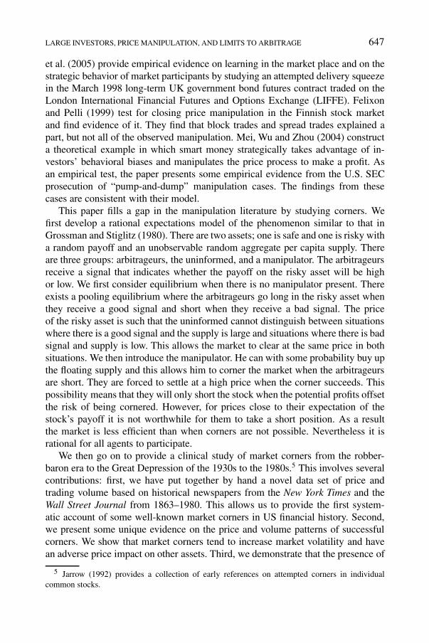
The equilibrium is shown in Figure 4. For P ∗ > P ≥ P2, there are no shortsales. The arbitrageurs get bad news but are unwilling to take a short position. Thusthe uninformed must hold all of the risky assets and the arbitrageurs hold nothing.Pooling still occurs though. The uninformed still cannot distinguish between goodnews and a high x and bad news and a low x, it is just the x is not as low as before.The line marked “Bad News” represents what happens now when the arbitrageursreceive bad news. For P1 ≥ P ≥ P ∗, there are short sales as before. In this region
655

654 FRANKLIN ALLEN ET AL.
Figure 4. An equilibrium with corners.
there are corners π(1 − ϕ) of the time. The other change is that the revelation ofinformation near xH is reduced compared to Figure 3.
A comparison of Figures 3 and 4 demonstrates that the market is less efficientwhen there is a manipulator who may corner the market. When θ = θG, so thereis good news, the price of the risky asset is the same in both figures for all valuesof x. On the other hand, when θ = θB , so there is bad news, the price is only thesame in both cases when 0 ≤ x ≤ x1 and x3 ≤ x ≤ xH . For x1 ≤ x ≤ x3, the pricein Figure 4 is above the price in Figure 3. In other words, the price is farther awayfrom the expected payoff θB , so the market is less efficient when the possibility ofmanipulation exists.
Next consider the manipulator. We assume that the arbitrageurs have taken theirshort positions with the manipulator. A similar analysis holds if they have taken the
656

LARGE INVESTORS, PRICE MANIPULATION, AND LIMITS TO ARBITRAGE 655
short positions with somebody other than the manipulator. Given the manipulatoris risk neutral, his expected utility from undertaking the manipulation is
EUM = π{(1 − ϕ)0.5[(1 − λ)X∗APC + XMθB + XMθG]
+ ϕXMEθ − XMPM}. (24)
This expression can be understood as follows. There is a probability π that themanipulator will attempt to corner the market and a probability (1 − ϕ) that thiscorner will have the potential to succeed. Half of the time bad news will have beenreceived and in this case the manipulator will be able to force the arbitrageurs tosettle at PC on their shorted stock, (1−λ)X∗
A. The stock the manipulator purchasesfrom the uninformed, XM , pays off θB on average. The other half of the timegood news is received and the XM the manipulator purchases pays off θG. Theterm ϕXMEθ represents the expected payoff on the stock when the corner doesnot succeed. The final term XMPM is the cost of buying the risky asset from theuninformed.
Rearranging (24)
EUM = π{(1 − ϕ)0.5[(1 − λ)X∗APC] + XM(Eθ − PM)}. (25)
Next consider the determination of PM in (20). Since the first derivative of theleft hand side with respect to η is negative, putting η = 0 increases the left handside. Denoting the solution for PM for the case when η = 0, P ∗
M , it can be shown
P ∗M = Eθ − γ
2σ 2
ε > PM. (26)
Using this in (25) it follows that EUM > 0 so the manipulator is better off frommanipulating the market.
This analysis of the expected utilities of the uninformed, the arbitrageurs and themanipulator shows that corners can occur when everybody is behaving rationally.The uninformed have the same expected utility whether there are corners or not.The arbitrageurs and the manipulator are better off from participating in the market.
The model presented in this section has a number of implications that areconsidered in the empirical section below. The first part of this investigates thedifferences between successful and unsuccessful corners. Based on the analysisabove the results of this comparison are able to give some insight into the factorsthat are responsible for corners failing. If it is because the manipulator is unableto buy up the existing floating supply then volume will be higher for successfulcorners. On the other hand if it is because new floating supply comes on to themarket then volume will be higher for unsuccessful corners. In addition it can beseen from Figure 4 that the theory predicts that for successful corners the arbit-rageurs will be trading based on their information before a corner occurs. We testwhether this is the case or not. Finally, the model suggests that corners only occur
657

656 FRANKLIN ALLEN ET AL.
when there is bad news. We consider evidence whether or not this is the case in thecorners we investigate.
3. Historical Data and Institutional Background
One of the main hurdles in studying market manipulation is that the data are hard toobtain since the activity is often illegal and thus the participants do their best to hideit. Aggarwal and Wu (2006) and Mei et al. (2004) get around this problem by usingprosecution cases filed by the SEC. This paper overcomes the hurdle by lookingat a special form of manipulation – market corners. We identify market cornersby going through the stock market chronology compiled by Wyckoff (1972). Hedefines a corner as “a market condition brought about intentionally – though some-times accidentally – when virtually all of the purchasable, or floating, supply of acompany’s stock is held by an individual, or group, who are thus able to dictatethe price when settlement is called”. Thus, a corner is an extreme form of shortsqueeze, when the buy side has almost complete control of all floating shares.
We double check all the corners reported by Wyckoff (1972) using reports byBrooks (1969), Clews (1888), Sobel (1965), Stedman (1905), and Thomas (1989).We eliminate those that cannot be verified independently and we restrict our casesto those that happened between 1863 and 1928, because trading data were notavailable before 1863. The New York Stock Exchange passed rules to discouragemarket corners in 1920, after which only one corner was reported (Piggly-Wiggly)while the RCA corner in 1928 was unplanned.6 This gives a total of thirteen repor-ted cases of stock corners. In addition, we also include the case of the failed silvercorner of the Hunt brothers in 1980. The corners considered are shown in Table I.
We hand-collected the data set of price and trading volume from the New YorkTimes and we use the Wall Street Journal to search for information that is missingdue to the poor publication quality of historical newspapers. This is a laboriousprocess since we also need to aggregate trade-by-trade information in order to getdaily price and trading volume.7 Based on Wyckoff’s definition, we break cornersinto two categories: successful and failed corners. Successful corners are thosewhere the manipulator controlled almost all of the floating shares during the shortsqueeze and were able to dictate prices. Failed corners are those where the manip-ulators attempted but failed to control the large amount of floating shares eitherbecause of large amounts of new shares that were brought to the market on thesettlement date or because of government action. The corner dates are determinedbased on either the settlement call made by the manipulators or government action
6 Strictly speaking, the RCA corner is more like a short squeeze because no settlement was called.The reason we included it is because the manipulator Durant was reported to have controlled thewhole float.
7 Unfortunately, while the New York Times reports every trade for each stock before 1900, thetrades were not time-stamped so that we cannot perform microstructure studies.
658

LARGE INVESTORS, PRICE MANIPULATION, AND LIMITS TO ARBITRAGE 657
Table I. The sample of corners
We define the corner date as the date when shares that were sold short are called bythe manipulator. Corner dates have been established as found in the references, in particular,Clews (1888), Flynn (1934), Thomas (1989), and Wycoff (1968, 1972). Alongside the cornerdate we have characterized the outcome of the corner as successful or failed. For the StutzMotor Company and the Piggly-Wiggly Company, we do not have observations after thecorner date, due to the institutional halt in trading for both stocks, shortly prior to the cornerdate. Instead, for these stocks we report the results only for the period until the end of trading.
Company name Corner date Corner status
Harlem
1863 08/24/1863 Successful
1864 05/17/1864 Successful
Prairie du Chien 11/06/1865 Successful
Michigan Southern 04/04/1866 Successful
Erie Railroads
March – 1868 03/10/1868 Failed
November – 1868 11/16/1868 Successful
American Gold Coin 09/24/1869 Failed
Erie Railroads, 1872 09/17/1872 Failed
Northwestern 11/23/1872 Successful
Northern Pacific 05/09/1901 Successful
Stutz Motor 04/26/1920 Successful
Piggly Wiggly 03/20/1923 Successful
RCA 03/13/1928 Successful
Silver “Corner”, 1980 01/21/1980 Failed
dates. Appendix A provides a brief account of most of the corners while AppendixB provides a graphical depiction of their trading activity around the corner dates.
There are several common features of these corners. First of all, most cornersinvolved the robber-barons of the time, namely, Jay Gould, Daniel Drew, Jim Fisk,Cornelius Vanderbilt, and J. P. Morgan. Many of them were in a special position toexploit unwary investors – in many cases they were corporate officers/insiders aswell as large stockholders.8 Second, manipulators often controlled a huge amountof the common shares, often exceeding the whole float at the time of settlement,which put them in a position to dictate the settlement price to the short sellers.Third, stock prices tend to be discontinuous for cornered stocks, often with largeprice jumps around the corner date, suggesting major disruptions to an orderly
8 For example, as director of Erie, Drew had used his position to issue new shares to cover hisshort position. He also had hidden convertible bonds that were unknown to the market but wereconvertible to common when he was cornered.
659

658 FRANKLIN ALLEN ET AL.
market. Fourth, the amount of wealth controlled by the manipulators was largecompared to the market cap of the stock.9
The presence of deep-pocketed manipulators makes short-selling an extremelyhazardous venture for would-be arbitrageurs. The oldest and most sacred rule ofWall Street at the time was “He who sells what isn’t his, Must buy it back or go toprison”. As pointed out by Jones and Lamont (2002), there are two main risks forshort sellers: first, short sellers are required to post additional collateral if the priceof the shorted stock rises. Second, stock loans can be called at the discretion of thelender, giving rise to recall risk.
Manipulation will exacerbate the above risks and add some new risks to thearbitrageurs. First of all, when manipulators are better informed about the supplyof shares, the short sellers are more likely to close their position at a loss. The lenderof the stock would demand the return of her shares at the worst possible time. Thestock lender/ manipulator will call in her loan when the shares have risen in priceand the short sellers are unable to find shares to borrow. Second, deep-pocketedmanipulators will be able to drive stock prices to the point where short sellerswould not be able to post additional collateral and thus have to close their positionat a loss. Third, the price jumps during a market corner create a huge operationalrisk for brokers who arrange stock borrowing for short sellers. In the event of amarket corner, large jumps in stock price could easily wipe out the collateral putup by short sellers and lead to severe financial losses for the broker in the event ofshort seller default.10 In this case, because of lack of liquidity in the market, it maybe difficult for brokers to protect themselves by closing short-sellers’ positions.
What institutional features made corners much more prevalent in the 19th cen-tury? First, it was easier to take a large short position then. According to JohnGordon, at the time “most short sales were effected not by borrowing the stock asis done today, but by using seller’s options. Stock was often sold for future deliverywithin a specified time, usually ten, twenty, or thirty days, with the precise time ofdelivery up to either the buyer – in which case it was called a buyer’s option –or the seller. . . . These options differed from modern options – puts and calls –in that the puts and calls convey only a right, not an obligation, to complete thecontract”.11 Since many short sellers often sold large quantities of naked options,the manipulator, having acquired the float, could force a corner by exercising hisbuyer’s option for immediate delivery and waiting for delivery from those who
9 According to Gordon (1999), Vanderbilt put together a stock pool of $5 million in cash tooperate the second Harlem corner. At the time, he already owned a big chunk of Harlem stocks dueto the first Harlem corner. On March 29, 1864, Harlem had a market capitalization of $11.9millionwith 110,000 shares outstanding. By the end of April, Vanderbilt and his allies owned 137,000 shares,with the difference sold to them by the short sellers. At time of his death in 1877, Vanderbilt left anestate that was worth $90 million.
10 In the second Harlem corner, Vanderbilt was so furious at the short sellers that he was reportedplanning to drive the stock price to $1,000. But he dropped his plan after leaning that it wouldbankrupt almost all brokerage firms on the street. See Clews (1888), chapter 34.
11 See Gordon (1999, p. 105).
660

LARGE INVESTORS, PRICE MANIPULATION, AND LIMITS TO ARBITRAGE 659
sold the seller’s option when the contract was due. Vanderbilt was said to havebought up all floating shares as well as all seller’s options during the Hudson Rivercorner.12
Second, margin requirements were less restrictive. Prior to 1934 when the Se-curities Act was enacted, this requirement was negotiated between the brokers andtheir clients. It could sometimes drop to as low as 10%, which allowed a manip-ulator to acquire a large block of stocks with relatively little capital.13 Third, themarket was opaque and there was little disclosure of corporate equity informa-tion. Thus, the general public had little knowledge about the float of the stockas well as who were the major shareholders and their positions. As a result, theshort sellers could have a false sense of security by shorting a stock, not realizingthat the float was much smaller than they had thought. Fourth, poor transportationmade it difficult for out of town and overseas investors to bring their shares tothe market, effectively taking those shares out of the float.14 According to Sobel(1988), foreigners owned $243 million of railroad securities in 1869. Fifth, thelegal system was much less independent and judges could often be bribed to issueinjunctions to restrict the issue of new shares.15 By controlling the supply of shares,it made it easier for the manipulator to achieve a corner. Finally, there was a blatantdisregard for conflict of interest and minority shareholder rights. Directors oftentook advantage of their position to manipulate stock price. Because of their abilityto restrict the supply of shares, this made corners much more likely to happen inthe 19th century.16
Several legal and regulatory developments made corners more difficult. First,early on in our sample period the NYSE and Open Board rule of Nov. 30, 1868required corporations to register all securities sold at the exchange and providethirty-day notice on any new issues.17 Thus, the float of a company’s stock becamemuch more transparent. Second, the legislative committee of the NYSE launchedan investigation of corners, indicating an increasing concern of the members onthe negative impact of corners on market transactions.18 Third, the 1934 SecuritiesAct imposed a mandatory margin requirement, which increased the capital neededfor acquiring a large block of stocks. Fourth, the 1968 Williams Act required thefiling by any person or group of persons who have acquired a beneficial ownershipof more than five percent of equity of certain issuers within ten days of such an ac-quisition. This brings transparency to the ownership position of large shareholders.Lastly, the Governing Committee of the New York Stock Exchange delisted StutzMotor after its corner in 1920, effectively voiding the contract between short sellers
12 See Gordon (1999, pp. 105–106).13 See Wyckoff (1972, p. 239).14 See Sobel (1988, p. 161).15 See Sobel (1988, pp. 154–196) and Gordon (1999, p. 116).16 See Gordon (1999, p. 114).17 See Gordon (1999, p. 124).18 See Wyckoff (1972, p. 29).
661

660 FRANKLIN ALLEN ET AL.
and the manipulator. Moreover, delisting prevented manipulators from unwindingtheir position at the stock exchange after the corner.19 While manipulators maystill profit from the high prices short-sellers have to pay for the borrowed shares,they lose the liquidity to sell their vast holdings afterwards. As a result, the Stutzmotor corner was essentially the last intentional corner at the New York StockExchange.20
4. Empirical Results
The data for this study is collected from historical records of the New York Timesand The Wall Street Journal (see Table I for the corresponding time periods). Nineof the documented corners took place in the second half of the nineteenth centuryand five took place throughout the twentieth century. A concise historical referenceon each of these corners is presented in Appendix A. In the process of building thehistorical trading database we have aggregated intra-day transactions on a dailybasis.
We start with brief descriptive statistics for the companies in our sample. Weexamine daily returns, volatility, autocorrelation, price dispersion, and tradingvolume. We conduct this analysis for the pre-corner period, as well as in two cornersub-periods: corner period one – ten days before the corner to the corner date (in-cluded), and corner period two – the day after the corner date to ten days followingit. We present descriptive statistics for the returns for these periods in Table II.21
Notice that there is a significant increase in daily returns during corner period one(3.6%) as compared to the pre-corner period (0.4%), and a subsequent decline inreturns in corner period two (−2.7%). One notable example is the Northwesternmarket corner – in the first corner sub-period daily returns were 9.3% on average,while in the post-corner period the average daily return was −9.7%. The return iscontinuously compounded for the duration of the corner period and is computedusing the closing price.
There is a significant increase in the volatility of returns in both corner periods(7.3% for corner period one, and 6.7% for corner period two) as compared with thepre-corner period (3%). Another indicator of interest is the increased price disper-sion (7.1% for corner period one, and 4.3% for corner period two as compared tothe periods before the corner 3.1%). Price dispersion is defined as the daily spreadbetween high and low as a percentage of the close price. The evidence on theimpact of the market corner on price dispersion is consistent with the hypothesisthat there exists significant private information trading in the run-up to the corneras predicted by our model – as a result the price dispersion increases in the first
19 See Gordon (1999, pp. 217–218) and Brooks (1969, pp. 29–33).20 See Wyckoff (1972, p. 72).21 The pre-corner period has been standardized to have the length of 55 trading days, i.e., we define
it as [t −65, t −10). All of our results are robust to alternative pre-corner period length specification,e.g., 40 days as in [t − 65, t − 25) and correspondingly corner period one in [t − 25, t].
662

LARGE INVESTORS, PRICE MANIPULATION, AND LIMITS TO ARBITRAGE 661Ta
ble
II.
The
retu
rns,
pric
edi
sper
sion
,and
trad
ing
volu
me
arou
ndco
rner
s
The
corn
erpe
riod
isde
fine
das
[t−
10,t
+10
]day
sar
ound
the
corn
erda
te,
t,a
tota
lof
twen
ty-o
neda
ys,
incl
udin
gth
eco
rner
date
.T
henu
mbe
rof
obse
rvat
ions
refl
ects
the
num
ber
ofno
n-m
issi
ngda
ily
retu
rnob
serv
atio
ns.
Ret
urn
isde
fine
das
the
cont
inuo
usly
com
poun
ded
retu
rnco
mpu
ted
from
the
clos
epr
ice.
Sha
revo
lum
eis
defi
ned
asth
eto
taln
umbe
rof
shar
estr
aded
inth
eco
rres
pond
ing
trad
ing
day.
Dai
lytu
rnov
eris
defi
ned
asth
era
tio
ofth
eto
tal
num
ber
ofsh
ares
trad
eddi
vide
dby
the
tota
lnu
mbe
rof
outs
tand
ing
shar
es.
Aut
ocor
rela
tion
refe
rsto
the
auto
corr
elat
ion
ofre
turn
sco
mpu
ted
wit
hin
the
corr
espo
ndin
gpe
riod
(dif
fers
acro
sspa
nels
A,B
,and
C),
ρt
=co
rr(R
t,R
t−1)
.Pri
cedi
sper
sion
refe
rsto
the
diff
eren
cebe
twee
nhi
ghan
dlo
w,s
cale
dw
ithth
ecl
ose
pric
efo
rea
chtr
adin
gda
y.Fo
rS
tutz
Mot
or,w
eha
vede
fine
dth
eco
rner
peri
odst
arti
ngda
teas
10da
yspr
ior
toth
ede
cisi
onto
halt
the
trad
ing
ofth
eco
mpa
nyst
ock,
sinc
eit
sco
rner
date
isaf
ter
the
offi
cial
halt
oftr
adin
g.T
hepr
e-co
rner
peri
odis
defi
ned
asth
epe
riod
the
sixt
yfi
fth
day
thro
ugh
the
elev
enth
day
befo
reth
eco
rner
date
.The
firs
tco
rner
sub-
peri
odis
defi
ned
asth
epe
riod
ten
days
befo
reth
eco
rner
date
unti
lth
eco
rner
date
(inc
lude
d).T
hese
cond
corn
ersu
b-pe
riod
isde
fine
das
the
peri
odfr
omth
efi
rstd
ayfo
llow
ing
the
corn
erto
the
tent
hda
yfo
llow
ing
the
corn
erda
te.
Pane
lA:P
re-c
orne
rpe
riod
,[t−
65,t−
10]
Dai
lyD
aily
pric
eD
aily
shar
esD
aily
Dai
lyre
turn
disp
ersi
ontr
aded
turn
over
auto
corr
.N
Mea
nSt
d.M
ean
Std.
dev
Mea
nSt
d.M
ean
Std.
ρ1,
cs
dev
(%)
(%)
dev
dev
Har
lem
,186
354
0.00
60.
060
4.2%
3.9%
11,2
328,
070
0.10
20.
073
−0.1
77H
arle
m,1
864
550.
010
0.05
45.
1%3.
8%10
,888
8,57
90.
099
0.07
8−0
.200
Prai
rie
duC
hien
550.
008
0.03
02.
5%2.
0%1,
280
1,24
90.
043
0.04
20.
040
Mic
higa
nSo
uthe
rn55
0.00
30.
018
3.4%
6.8%
12,3
554,
794
––
−0.3
79E
rie,
03–
1868
53−0
.002
0.01
51.
8%1.
4%17
,214
9,50
40.
297
0.16
40.
102
Eri
e,11
–18
6855
−0.0
020.
028
2.8%
1.5%
7,67
17,
692
0.03
80.
038
0.19
4G
old
Coi
n,18
6955
0.00
00.
005
––
––
––
0.14
3E
rie,
1872
53−0
.002
0.02
65.
2%17
.0%
19,3
6013
,490
0.11
70.
081
−0.1
45N
orth
wes
tern
540.
002
0.03
12.
6%2.
2%18
,908
16,6
930.
105
0.09
2−0
.411
Nor
ther
nPa
cific
550.
004
0.01
41.
9%1.
3%37
,714
33,4
130.
047
0.04
2−0
.125
Stut
zM
otor
550.
008
0.03
93.
1%3.
2%97
61,
002
0.01
00.
010
0.20
3Pi
ggly
Wig
gly
550.
006
0.03
52.
1%1.
6%2,
175
2,13
90.
011
0.01
1−0
.215
RC
A55
0.00
00.
022
3.1%
1.4%
75,5
9649
,872
0.06
50.
043
−0.0
33Si
lver
“Cor
ner”
540.
011
0.04
02.
3%2.
1%7,
263
4,89
5–
–−0
.076
Mea
n55
0.00
40.
030
3.1%
3.7%
0.08
5−0
.077
663

662 FRANKLIN ALLEN ET AL.
Tabl
eII
.T
here
turn
s,pr
ice
disp
ersi
on,a
ndtr
adin
gvo
lum
ear
ound
corn
ers
(con
tinu
ed)
Pane
lB:C
orne
r-pe
riod
,[t−
10,t]
Dai
lyD
aily
pric
eD
aily
shar
esD
aily
Dai
ly
retu
rndi
sper
sion
trad
edtu
rnov
erau
toco
rr.
Mea
nS
td.
Mea
nS
td.d
evM
ean
Std
.M
ean
Std
.ρ
1,cs
dev
(%)
(%)
dev
dev
Har
lem
,186
30.
019
0.04
13.
2%1.
7%8,
459
4,09
20.
077
0.03
70.
131
Har
lem
,186
40.
018
0.03
11.
0%1.
5%77
367
20.
007
0.00
6−0
.194
Pra
irie
duC
hien
0.09
50.
216
14.2
%15
.1%
3,94
41,
905
0.13
20.
064
−0.2
43
Mic
higa
nS
outh
ern
0.00
90.
014
4.9%
3.7%
14,1
747,
765
––
−0.0
20
Eri
e,03
–18
680.
009
0.03
14.
2%2.
4%24
,462
14,6
480.
422
0.25
30.
026
Eri
e,11
–18
680.
021
0.08
15.
1%2.
9%14
,402
18,5
730.
072
0.09
30.
713
Gol
dC
oin,
1869
−0.0
020.
025
––
––
––
−0.2
85
Eri
e,18
720.
006
0.02
44.
4%3.
2%23
,600
14,3
320.
142
0.08
6−0
.298
Nor
thw
este
rn0.
093
0.16
911
.4%
19.2
%7,
536
5,64
80.
042
0.03
10.
525
Nor
ther
nPa
cifi
c0.
102
0.21
022
.0%
47.2
%11
9,18
511
2,59
90.
149
0.14
10.
522
Stu
tzM
otor
0.06
60.
050
7.3%
2.9%
3,58
51,
971
0.03
60.
020
−0.2
43
Pig
gly
Wig
gly
0.00
50.
069
8.7%
17.8
%3,
982
6,66
80.
020
0.03
3−0
.119
RC
A0.
039
0.05
35.
7%4.
4%19
4,04
512
7,33
10.
168
0.11
00.
671
Sil
ver
“Cor
ner”
0.02
30.
013
0.0%
0.0%
9,34
75,
379
––
−0.0
59
Mea
n0.
036
0.07
37.
1%9.
4%0.
115
0.08
1
664

LARGE INVESTORS, PRICE MANIPULATION, AND LIMITS TO ARBITRAGE 663
Tabl
eII
.T
here
turn
s,pr
ice
disp
ersi
on,a
ndtr
adin
gvo
lum
ear
ound
corn
ers
(con
tinu
ed)
Pane
lC:C
orne
r-pe
riod
two,
[t+1,
t+
10]
Dai
lyD
aily
pric
eD
aily
shar
esD
aily
Dai
ly
retu
rndi
sper
sion
trad
edtu
rnov
erau
toco
rr.
Mea
nS
td.
Mea
nS
td.d
evM
ean
Std
.M
ean
Std
.ρ
1,cs
dev
(%)
(%)
dev
dev
Har
lem
,186
3−0
.032
0.03
74.
8%5.
3%6,
681
2,97
10.
061
0.02
70.
672
Har
lem
,186
40.
000
0.00
70.
3%0.
4%37
521
00.
003
0.00
2−0
.412
Pra
irie
duC
hien
−0.0
560.
149
2.3%
4.7%
526
468
0.01
80.
016
−0.1
96
Mic
higa
nS
outh
ern
−0.0
110.
020
3.5%
7.4%
6,60
05,
046
––
0.06
2
Eri
e,03
–18
68−0
.004
0.02
93.
0%1.
7%16
,003
8,45
00.
101
0.05
30.
394
Eri
e,11
–18
68−0
.025
0.02
910
.9%
12.2
%6,
803
8,06
50.
034
0.04
0−0
.193
Gol
dC
oin,
1869
−0.0
020.
009
––
––
––
−0.0
33
Eri
e,18
72−0
.006
0.03
26.
1%3.
8%20
,236
14,8
240.
122
0.08
9−0
.064
Nor
thw
este
rn−0
.097
0.18
34.
7%10
.9%
2,22
22,
176
0.01
20.
012
0.32
1
Nor
ther
nPa
cific
−0.0
710.
251
3.6%
2.9%
938
660
0.00
10.
001
−0.7
48
Stu
tzM
otor
––
––
––
––
–
Pig
gly
Wig
gly
––
––
––
––
–
RC
A0.
003
0.04
77.
0%3.
4%98
,040
71,1
100.
085
0.06
2−0
.154
Silv
er“C
orne
r”−0
.019
0.01
50.
7%1.
2%5,
097
4,25
5–
–−0
.309
Mea
n−0
.027
0.06
74.
3%4.
9%0.
049
−0.0
55
665

664 FRANKLIN ALLEN ET AL.
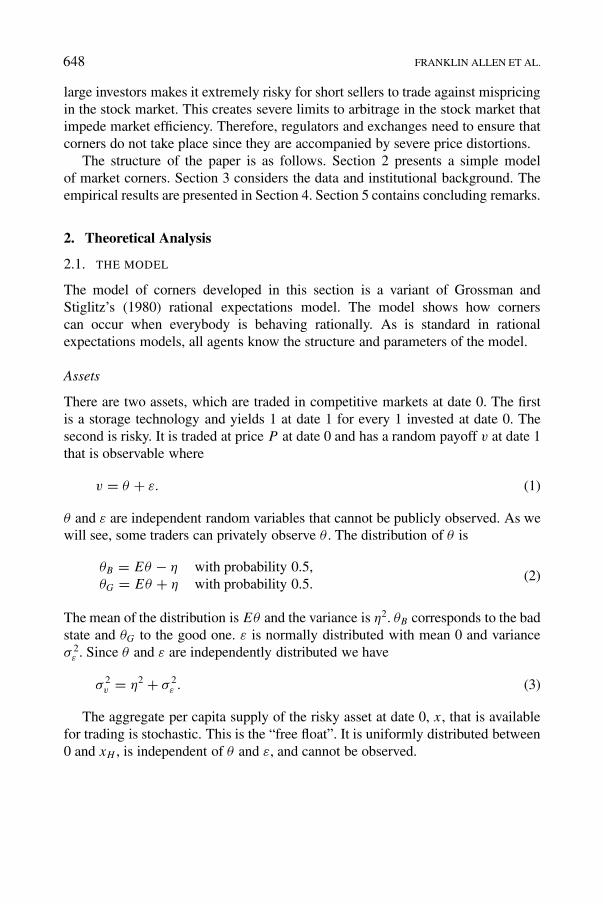
Figure 5. Cumulative abnormal trading volume (standardized). Abnormal trading volume isdefined as the difference between daily volume in the corner period and the pre-corner periodaverage daily trading volume. We standardize this variable with the standard deviation of thepre-corner period daily volume. In the figure, we have accumulated the trading volume acrossthe corner period, i.e., at date t − 10 we have plotted the abnormal trading volume at that day,at date t − 9 we have plotted the sum of the variable values at dates t − 10 and t − 9, etc.
period preceding the corner, while it substantially decreases in the period after thecorner. For example, in the corner of Northern Pacific price dispersion prior to thecorner period is on average 1.9% daily. However, in the first corner sub-period,the price dispersion increases to 22% only to retreat to the low 3.6% following thecorner.
Table II also shows a significant change in trading volume between the pre-corner and the corner periods. For example, the average daily share volume hasincreased between pre-corner period to corner period one from 75,596 shares forRCA to 194,045 or from 37,714 to 119,185 for Northern Pacific, or from 7,671 to14,402 for the second Erie corner. Even more dramatic was the dry-up of liquid-ity after the corner date for some stocks, e.g., a decrease from 119,263 shares incorner period one to 938 shares in corner period two for Northern Pacific. Figure 5provides plots of changing liquidity (we use cumulative abnormal trading volumeas a proxy). The abnormal trading volume is defined as the difference between dailyvolume in the corner period and average daily trading volume in the pre-cornerperiod. We standardize this variable with the standard deviation of the pre-cornerperiod daily volume. In the figure, we have accumulated the trading volume acrossthe corner period, i.e., at day t − 10 (i.e., ten days prior to the corner date) we haveplotted the abnormal trading volume at that date; at day t − 9 we have plotted thesum of the abnormal trading volume at days t − 10 and t − 9, etc.
A clear pattern of increased turnover and subsequent gradual decrease isdisplayed in Figure 5. However, the pattern of liquidity impact differs across suc-cessful and failed corners, being more pronounced for the successful corners as
666

LARGE INVESTORS, PRICE MANIPULATION, AND LIMITS TO ARBITRAGE 665
compared to the failed ones. This is consistent with the hypothesis that successfulmarket corners have a considerable impact on the liquidity of the cornered stock.As discussed in Section 2 it also suggests that corners failed due to an inability topurchase all the floating supply rather than because of new shares being added tothe floating supply.
We further tabulate in Table II the turnover around the corner events. Dailyturnover is defined as the ratio of the total number of shares traded divided bythe total number of outstanding shares.22 Comparing Table II, panels A and B,there is an increase in the average daily turnover between the pre-corner period andcorner period one (from 0.085 to 0.115). However, a Wilcoxon test of the equalityof the means of the average turnover in pre-corner period and in corner periodone cannot reject the null hypothesis of equality of the means (p-value is 0.53).Similarly, comparing panels B and C of Table II, there is a decrease in the averagedaily turnover in the corner period two (0.049) as compared with corner periodone (0.115). A Wilcoxon test of equality of the means of corner period one andcorner period two rejects the null hypothesis of equality of the means at the 10%significance level (p-value is 0.07). One caveat in our interpretation of turnoverresults above is that the available float may be much smaller than the outstandingfloat. Thus, such comparisons of daily turnover before and during the corner eventmight be difficult to interpret.
We also analyze autocorrelation patterns in Table II. Daily price changes shouldbe serially uncorrelated if a market is efficient. There seems to be a significantchange in autocorrelation of returns between pre-corner and corner periods. In thefirst corner period we observe on average a positive autocorrelation of 8.1%, ascompared with the second corner sub-period, where the autocorrelation is −5.5%.The pre-corner autocorrelation is −7.7%. The pattern of autocorrelation within thecorner period one is suggestive of the presence of informed trading in the sense ofLlorente et al. (2002). This is investigated further below.
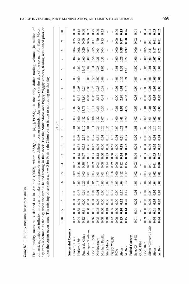
One of the predictions of our theoretical model is that corners would have alarge impact on liquidity. To test this prediction, we have examined in Table III theproperties of a measure of illiquidity, similar to the one in Amihud (2002):
ILLIQi,t = |Ri,t |/VOLDi,t , (27)
where VOLDi,t is the daily dollar trading volume (in million of dollars) for cornerstock i in day t , adjusted for inflation.23 Higher values of this measure indicate
22 We are able to retrieve historical data on the outstanding shares for all companies exceptMichigan Southern. There are two cases where the corner event was followed by a stock issue.In the case of Erie market corner of March 1868 there were 100,000 new shares issued immediatelyafter the corner date. In the case of the Erie market corner of November 1868 there were records ofseveral fraudulent over-issues of that stock, see New York Times as of 03/10/1868 and 11/16/1868.
23 For all stocks VOLDi,t is defined as the product of the close price and the number of sharestraded (in millions), adjusted for inflation. For the NYMEX 5000 oz silver futures contracts, wedefine it as: VOLDsilver,t = Nt × 5000 × Pt /108, where Nt is the number of futures contracts
667

666 FRANKLIN ALLEN ET AL.
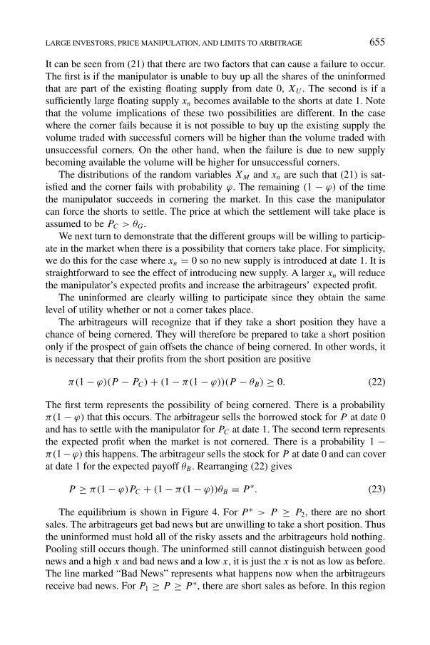
lower liquidity, i.e., little trading volume leads to more significant stock pricechanges (the average correlation of the illiquidity measure and the standardizedabnormal volume over [t − 10, t + 10] is −0.27). The results in Table III indicatethat on average there is a decrease in liquidity after the corner date, where thiseffect is stronger for successful corners.24 We illustrate this pattern in Figure 6,where we display the average daily illiquidity measure across successful and failedcorner stocks,
AILLIQt = 1
N
N∑
i
|Ri,t |/VOLDi,t .25
The figure shows the increased illiquidity following the corner date, with greaterilliquidity for the successful corners.
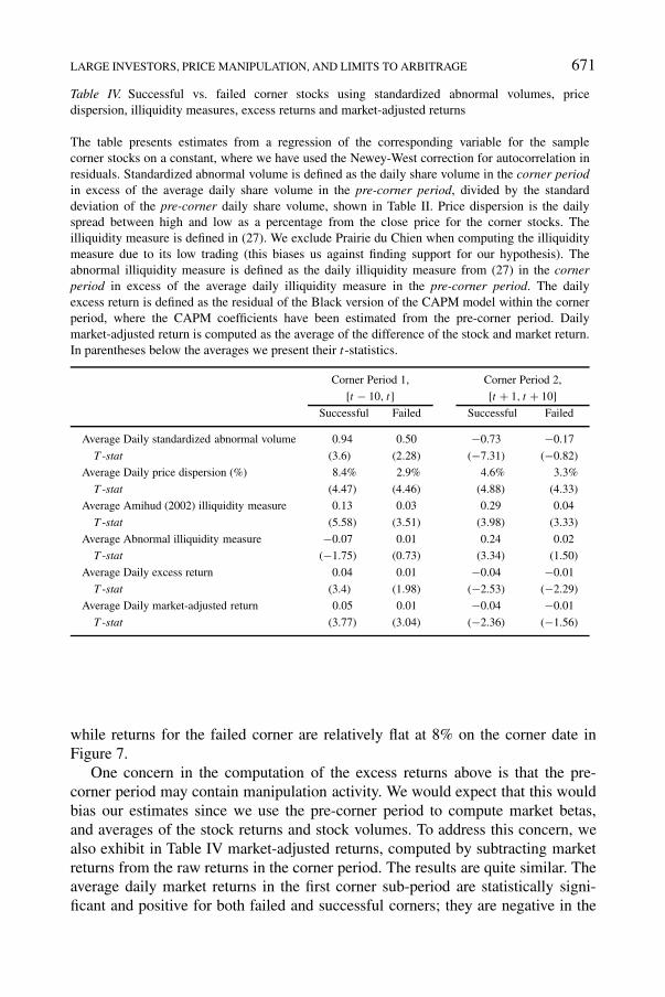
In Table IV we present a comparison of successful and failed corners. Thecomparison is based on standardized abnormal trading volume, price dispersion,stock illiquidity (defined in (27)), an abnormal illiquidity measure (defined be-low), excess returns, and market-adjusted returns. The table records coefficientestimates and corresponding t-statistics, based on a regression of each of theabove variables on a constant, where we use the Newey-West correction to addressautocorrelation-in-residuals concerns for the corner period 1 and for the cornerperiod 2.
traded in day t , and Pt is the close price (in cents per ounce) as of trading day t . We translatethis measure into millions US dollars and adjust it for inflation in order to make it comparableacross corners which occur in different time periods. The adjustment is based on the inflationconversion factors for the US dollar from 1863 to 1980 which we obtain from Robert Sahr, athttp://oregonstate.edu/dept/pol_sci/fac/sahr/sahr.htm. We express dollar values in US dollars as of1900.
24 There are two caveats associated with this measure. The first one is that we could not compute itfor days with zero trading volume. Second, this measure is very sensitive to changes in volume whenthe level of trading volume is low. For example, Prairie du Chien has substantially higher ILLIQt inthe post-corner period as compared to the other corner stocks, partly because of the thin trading ofits stock.
25 Note that in Figure 6 we have excluded the observations for Prairie du Chien. Due to its low trad-ing volume in the second corner period, the illiquidity measure for that stock is substantially higherthan the illiquidity measures for the rest of our sample corner stocks. The conservative approach wefollow would bias our results against finding support for our hypothesis that liquidity would decreaseafter the corner event and would further ascertain that our results are not driven by outliers.
668
LARGE INVESTORS, PRICE MANIPULATION, AND LIMITS TO ARBITRAGE 667Ta
ble
III.
Illi
quid
ity
mea
sure
for
corn
erst
ocks
The
illiq
uidi
tym
easu
reis
defi
ned
asin
Am
ihud
(200
2),
whe
reIL
LIQ
i,t
=|R
i,t|/V
OL
Di,t
isth
eda
ily
doll
artr
adin
gvo
lum
e(i
nm
illi
onof
dolla
rs),
adju
sted
for
infl
atio
nin
orde
rto
mak
eit
com
para
ble
acro
ssdi
ffer
ent
corn
erpe
riod
s.D
ayze
ro(i
.e.,
t)is
the
day
ofth
eco
rner
.For
Stu
tzM
otor
,da
yze
rois
defi
ned
asth
eda
yw
hen
the
NY
SE
halt
edtr
adin
gin
that
stoc
k.Fo
rth
eS
tutz
Mot
oran
dP
iggl
yW
iggl
yco
rner
s,tr
adin
gw
asha
lted
prio
ror
upon
the
corn
eroc
curr
ence
.The
mis
sing
obse
rvat
ion
att=
5fo
rP
rair
iedu
Chi
enco
rner
isdu
eto
notr
adin
gon
that
day.
Day
t
−10
−9−8
−7−6
−5−4
−3−2
−10
12
34
56
78
910
Succ
essf
ulC
orne
rsH
arle
m,1
863
0.12
0.00
0.01
0.06
0.05
0.09
0.07
0.03
0.05
0.02
0.01
0.03
0.02
0.02
0.01
0.03
0.02
0.04
0.04
0.25
0.08
Har
lem
,186
40.
040.
380.
910.
430.
000.
530.
160.
180.
320.
050.
000.
000.
660.
320.
080.
000.
000.
040.
080.
120.
12
Prai
rie
duC
hien
0.42
0.31
0.00
0.39
0.26
0.05
0.50
0.67
0.55
2.35
1.12
0.82
13.7
318
.80
6.24
–34
.45
0.60
0.20
0.00
0.00
Mic
higa
nSo
uthe
rn0.
010.
000.
010.
000.
040.
010.
020.
010.
060.
060.
010.
050.
130.
030.
030.
020.
070.
020.
020.
060.
02
Eri
e,11
–18
680.
360.
010.
040.
040.
050.
030.
090.
230.
120.
270.
110.
080.
140.
060.
280.
590.
310.
582.
650.
710.
75
Nor
thw
este
rn0.
050.
030.
060.
010.
150.
010.
030.
120.
040.
540.
260.
220.
543.
170.
250.
070.
280.
210.
041.
700.
00
Nor
ther
nPa
cific
0.00
0.00
0.00
0.00
0.00
0.01
0.00
0.00
0.00
0.01
0.20
2.07
0.36
0.44
0.38
0.09
1.02
0.53
0.04
0.13
0.25
Stut
zM
otor
0.18
0.18
0.06
0.36
0.02
0.25
0.14
0.23
0.08
0.33
0.36
––
––
––
––
––
Pig
gly
Wig
gly
0.12
0.05
0.05
0.34
0.36
0.18
0.19
0.88
0.55
1.33
0.14
––
––
––
––
––
RC
A0.
000.
000.
000.
000.
000.
000.
000.
010.
000.
010.
000.
000.
010.
000.
010.
010.
010.
000.
000.
000.
00
Mea
n0.
130.
100.
120.
160.
090.
120.
120.
240.
180.
500.
220.
411.
952.
860.
910.
124.
520.
250.
380.
370.
15St
.Dev
.0.
150.
140.
280.
190.
120.
170.
150.
300.
220.
770.
340.
724.
776.
532.
160.
2112
.10
0.27
0.92
0.58
0.26
Fai
led
Cor
ners
Eri
e,03
–18
680.
010.
010.
020.
010.
060.
020.
020.
040.
010.
020.
010.
020.
050.
030.
060.
030.
020.
060.
060.
020.
01
Gol
d,18
69–
––
––
––
––
––
––
––
––
––
––
Eri
e,18
720.
090.
000.
050.
040.
040.
030.
010.
030.
040.
020.
020.
020.
010.
050.
000.
030.
050.
090.
050.
010.
04
Silv
er“C
orne
r”,1
980
0.01
0.01
0.01
0.00
0.02
0.01
0.01
0.01
0.01
0.00
0.27
0.01
0.01
0.01
0.01
0.01
0.01
0.04
0.41
0.01
0.04
Mea
n0.
040.
010.
030.
020.
040.
020.
010.
030.
020.
010.
100.
020.
020.
030.
030.
030.
030.
070.
170.
010.
03St
.Dev
.0.
040.
000.
020.
020.
020.
010.
000.
020.
020.
010.
150.
010.
030.
020.
030.
010.
020.
030.
210.
010.
02
669
668 FRANKLIN ALLEN ET AL.
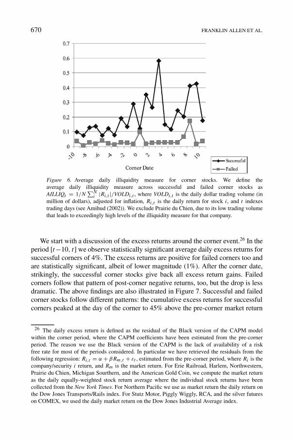
Figure 6. Average daily illiquidity measure for corner stocks. We define theaverage daily illiquidity measure across successful and failed corner stocks asAILLIQt = 1/N
∑Ni |Ri,t |/VOLDi,t , where VOLDi,t is the daily dollar trading volume (in
million of dollars), adjusted for inflation, Ri,t is the daily return for stock i, and t indexestrading days (see Amihud (2002)). We exclude Prairie du Chien, due to its low trading volumethat leads to exceedingly high levels of the illiquidity measure for that company.
We start with a discussion of the excess returns around the corner event.26 In theperiod [t−10, t] we observe statistically significant average daily excess returns forsuccessful corners of 4%. The excess returns are positive for failed corners too andare statistically significant, albeit of lower magnitude (1%). After the corner date,strikingly, the successful corner stocks give back all excess return gains. Failedcorners follow that pattern of post-corner negative returns, too, but the drop is lessdramatic. The above findings are also illustrated in Figure 7. Successful and failedcorner stocks follow different patterns: the cumulative excess returns for successfulcorners peaked at the day of the corner to 45% above the pre-corner market return
26 The daily excess return is defined as the residual of the Black version of the CAPM modelwithin the corner period, where the CAPM coefficients have been estimated from the pre-cornerperiod. The reason we use the Black version of the CAPM is the lack of availability of a riskfree rate for most of the periods considered. In particular we have retrieved the residuals from thefollowing regression: Ri,t = α + βRm,t + εt , estimated from the pre-corner period, where Ri is thecompany/security i return, and Rm is the market return. For Erie Railroad, Harlem, Northwestern,Prairie du Chien, Michigan Sourthern, and the American Gold Coin, we compute the market returnas the daily equally-weighted stock return average where the individual stock returns have beencollected from the New York Times. For Northern Pacific we use as market return the daily return onthe Dow Jones Transports/Rails index. For Stutz Motor, Piggly Wiggly, RCA, and the silver futureson COMEX, we used the daily market return on the Dow Jones Industrial Average index.
670
LARGE INVESTORS, PRICE MANIPULATION, AND LIMITS TO ARBITRAGE 669
Table IV. Successful vs. failed corner stocks using standardized abnormal volumes, pricedispersion, illiquidity measures, excess returns and market-adjusted returns
The table presents estimates from a regression of the corresponding variable for the samplecorner stocks on a constant, where we have used the Newey-West correction for autocorrelation inresiduals. Standardized abnormal volume is defined as the daily share volume in the corner periodin excess of the average daily share volume in the pre-corner period, divided by the standarddeviation of the pre-corner daily share volume, shown in Table II. Price dispersion is the dailyspread between high and low as a percentage from the close price for the corner stocks. Theilliquidity measure is defined in (27). We exclude Prairie du Chien when computing the illiquiditymeasure due to its low trading (this biases us against finding support for our hypothesis). Theabnormal illiquidity measure is defined as the daily illiquidity measure from (27) in the cornerperiod in excess of the average daily illiquidity measure in the pre-corner period. The dailyexcess return is defined as the residual of the Black version of the CAPM model within the cornerperiod, where the CAPM coefficients have been estimated from the pre-corner period. Dailymarket-adjusted return is computed as the average of the difference of the stock and market return.In parentheses below the averages we present their t-statistics.
Corner Period 1, Corner Period 2,
[t − 10, t] [t + 1, t + 10]Successful Failed Successful Failed
Average Daily standardized abnormal volume 0.94 0.50 −0.73 −0.17
T -stat (3.6) (2.28) (−7.31) (−0.82)
Average Daily price dispersion (%) 8.4% 2.9% 4.6% 3.3%
T -stat (4.47) (4.46) (4.88) (4.33)
Average Amihud (2002) illiquidity measure 0.13 0.03 0.29 0.04
T -stat (5.58) (3.51) (3.98) (3.33)
Average Abnormal illiquidity measure −0.07 0.01 0.24 0.02
T -stat (−1.75) (0.73) (3.34) (1.50)
Average Daily excess return 0.04 0.01 −0.04 −0.01
T -stat (3.4) (1.98) (−2.53) (−2.29)
Average Daily market-adjusted return 0.05 0.01 −0.04 −0.01
T -stat (3.77) (3.04) (−2.36) (−1.56)
while returns for the failed corner are relatively flat at 8% on the corner date inFigure 7.
One concern in the computation of the excess returns above is that the pre-corner period may contain manipulation activity. We would expect that this wouldbias our estimates since we use the pre-corner period to compute market betas,and averages of the stock returns and stock volumes. To address this concern, wealso exhibit in Table IV market-adjusted returns, computed by subtracting marketreturns from the raw returns in the corner period. The results are quite similar. Theaverage daily market returns in the first corner sub-period are statistically signi-ficant and positive for both failed and successful corners; they are negative in the
671

670 FRANKLIN ALLEN ET AL.
Figure 7. Cumulative excess returns. We exhibit the cumulative excess returns for cornerstocks. Excess return is defined as the residual of the regression: Ri,t = α + βRm,t + εt ,estimated for the pre-corner period, where Ri is the company i return, and Rm is the market re-turn. For Erie Railroad, Harlem, Northwestern, Prairie du Chien, Michigan Sourthern, and theAmerican Gold Coin, we compute the market return as the daily equally-weighted stock returnaverage where the individual stock returns have been collected from the New York Times. ForNorthern Pacific we use as market return the daily return on the Dow Jones Transports/Railsindex. For Stutz Motor, Piggly Wiggly, RCA, and the silver futures on COMEX, we used thedaily market return on the Dow Jones Industrial Average index.
second corner sub-period. The order of magnitude of the average market-adjustedreturns is similar to the one of the average excess returns.
Before the corner date, there is a significant rise in the abnormal volume ofsuccessful corner stocks, 0.94 standard deviations above the pre-corner averagedaily volumes. We observe the same result for failed corner stocks, but by lowermagnitude, 0.50. Strikingly, after the corner date we observe a sharp fall in tradingvolume, especially for successful corner stocks (0.73 standard deviations below thepre-corner average daily volumes).
Price dispersion increases before the corner especially for successful cornerstocks, by 8.4%. A similar increase is observed for failed corner stocks, but by less,2.9%. The price dispersion decreases following the corner for successful corners(4.6%), but it increases slightly for failed corners (3.3%). This pattern of increasedprice dispersion (reflective of information trading) is also displayed in Figure 8.The successful corner stocks have higher daily price dispersion compared to thefailed ones, reaching 36.2% on the date of the corner (for failed corners the pricedispersion is 5.5%). The large price dispersion in the case of successful corners isindicative of the presence of private information trading and it reflects the volatilenature of market corners.
We also study in Table IV the stock illiquidity around the corner date. We definestock illiquidity as in Equation (27). We exclude Prairie du Chien when computingthe illiquidity measure due to its low trading volume (low trading volume results in
672

LARGE INVESTORS, PRICE MANIPULATION, AND LIMITS TO ARBITRAGE 671
Figure 8. Daily price dispersion (high-low) as a percentage of closing prices. Daily pricedispersion is the difference between the high and low prices within a given trading day as apercentage of the close price.
exceedingly high values of the illiquidity measure). This biases us against findingsupport for our hypothesis of strong impact of the corner event on liquidity. Theresults in Table IV indicate that there is an increase in the illiquidity measure afterthe corner for both successful and failed stocks. The increase is more than twofold for successful corners: from 0.13 in the first corner sub-period to 0.29 in thesecond corner sub-period. Similarly, we observe an increase in the illiquidity forfailed corners, but by lower magnitude: from 0.03 in the first corner sub-period to0.04 in the second sub-corner period. Successful corners are subject to substantiallyhigher illiquidity following the corner as compared to failed ones. We further reporta measure of abnormal illiquidity, defined as the average of the daily illiquiditymeasure from Equation (27) in the corner period in excess of the average dailyilliquidity measure in the pre-corner period. When computing abnormal illiquid-ity we still exclude Prairie du Chien from the calculation, due to its low tradingvolume. Based on the abnormal illiquidity measure, it appears that illiquidity forfailed corners within corner periods one and two is not statistically different fromthe pre-corner value. The illiquidity for successful corners for corner period one isstatistically significantly lower than the illiquidity from the pre-corner period. Theilliquidity for successful corners in corner period two is statistically significantlyhigher than the illiquidity in the pre-corner period. This demonstrates the ability ofthe manipulator in successful corners to withhold the acquired free float after thecorner date, while at the same time make it freely available in the corner periodone.
In Table V we present daily market returns in the period [t − 10, t + 10]around the corner date. For Harlem, Prairie du Chien, Michigan Southern, Erie,Northwestern, and American Gold Coin we use as the market return the return on
673

672 FRANKLIN ALLEN ET AL.
Figure 9. Cumulative market return around corner date. We exhibit the cumulative marketreturn for all corner securities. In the figure, we have accumulated the market return across thecorner period, i.e., at date t − 10 we have plotted the market return at that day, at date t − 9we have plotted the sum of the market returns at dates t − 10 and t − 9, etc.
the equally weighted stocks returns, which was hand-collected from the FinancialAffairs section of the New York Times for the corresponding time period. At thetime, the companies included in that section were predominantly railroads. ForNorthern Pacific we use the Dow Jones Transports/ Rails Index. For Stutz Motor,Piggly Wiggly, and RCA we use the Dow Jones Industrials index. For the silvercorner, we use the Dow Jones Industrial Average Index. Daily returns are presentedin percentage value.
Results on market return are mixed. On average, the days following the cornerhad some of the largest decreases in returns. This spillover effect of the corner onthe market return is perhaps due to the fact that short-sellers pressed for liquiditymight start a fire sale of their portfolios thus causing an overall decline of marketreturns. The effect seems to be transient since the market generally rebounded bythe fourth day after the corner. Furthermore, we could see a pronounced increase inmarket volatility in the [t −1, t +1] period around the corner date. This increase ismore pronounced for successful corner stocks as compared to failed corner stocks.
The results from Table V are further illustrated in Figure 9 where we havepresented the cumulative market return around the corner date. As discussed abovethe impact of successful corners on market returns seems to be transient. However,the impact of failed corners on market returns seems to be more pronounced andpersistent.
In Table VI, we present a test of whether there is trading on private informationas in our theoretical model, based on the dynamic return-trading volume relation-
674

LARGE INVESTORS, PRICE MANIPULATION, AND LIMITS TO ARBITRAGE 673Ta
ble
V.M
arke
tdai
lyre
turn
arou
ndco
rner
date
s
We
pres
ent
the
dail
ym
arke
tre
turn
sin
the
peri
od[t
−10
,t
+10
]of
the
corn
erda
te.
For
Har
lem
,P
rair
iedu
Chi
en,
Mic
higa
nS
outh
ern,
Eri
e,N
orth
wes
tern
,and
Am
eric
anG
old
Coi
nw
eus
eas
mar
ket
retu
rnth
ere
turn
onth
eeq
uall
yw
eigh
ted
stoc
ksre
turn
sha
ndco
llec
ted
from
the
Fin
anci
alA
ffai
rsse
ctio
nof
the
New
York
Tim
es,f
orth
eco
rres
pond
ing
peri
od.A
tthe
tim
e,th
eco
mpa
nies
incl
uded
inth
atse
ctio
nw
ere
pred
omin
antl
yra
ilro
ads.
For
Nor
ther
nPa
cifi
cw
eus
eth
eD
owJo
nes
Tra
nspo
rts/
Rai
lsIn
dex.
For
Stu
tzM
otor
,P
iggl
yW
iggl
y,an
dR
CA
we
use
the
Dow
Jone
sIn
dust
rial
sin
dex.
For
the
silv
erco
rner
,we
use
the
Dow
Jone
sIn
dust
rial
Ave
rage
Inde
x.D
aily
retu
rns
are
pres
ente
din
perc
enta
geva
lue.
Day
t−1
0−9
−8−7
−6−5
−4−3
−2−1
01
23
45
67
89
10%
Succ
essf
ulC
orne
rsH
arle
m,1
863
−0.8
0.4
2.6
1.9
2.1
−0.3
−0.1
1.3
−0.2
0.0
1.8
0.2
−1.2
−0.3
0.0
0.9
−0.3
−1.0
−2.5
−6.2
0.9
Har
lem
,186
4−2
.0−2
.02.
0−0
.12.
31.
31.
2−0
.71.
33.
10.
11.
9−2
.40.
11.
8−0
.90.
50.
5−0
.5−0
.7−0
.1Pr
airi
edu
Chi
en,1
865
0.7
−0.1
0.7
1.3
0.5
−0.1
−0.5
0.5
−0.7
2.5
0.0
−1.4
0.4
−0.6
−0.5
−0.1
0.9
0.6
0.1
0.1
0.9
Mic
higa
nSo
uthe
rn,1
866
0.3
−0.2
−0.1
0.1
0.2
−0.3
−0.5
−0.8
0.4
0.1
0.6
−0.8
0.5
0.2
0.0
0.5
0.5
0.6
2.6
−1.3
0.5
Eri
e,11
–18
68−2
.4−3
.0−2
.53.
50.
0−0
.80.
2−0
.8−0
.53.
50.
7−1
.61.
3−0
.7−0
.3−0
.51.
4−0
.70.
61.
30.
0N
orth
wes
tern
,187
22.
0−0
.3−0
.4−0
.20.
7−0
.3−0
.41.
40.
83.
30.
90.
9−5
.10.
7−0
.10.
10.
1−0
.10.
10.
5−0
.8N
orth
ern
Paci
fic,1
901
0.7
1.7
0.6
1.3
−0.1
−1.3
0.3
0.9
−0.5
−4.8
−7.7
6.3
−0.4
−4.8
2.1
1.0
2.2
−0.1
−1.2
0.7
−0.2
Stut
zM
otor
,192
00.
5−0
.70.
3−0
.3−2
.5−2
.4−3
.61.
3−1
.80.
31.
5−0
.8−1
.7−1
.70.
40.
50.
30.
1−0
.3−0
.81.
4Pi
ggly
Wig
gly,
1923
−0.5
−0.2
−0.6
0.4
0.5
0.5
−0.5
−0.8
0.9
0.4
0.0
−0.1
−0.1
−1.1
−0.7
−0.9
0.7
0.4
−0.7
0.0
−1.2
RC
A,1
928
0.4
0.0
−0.1
0.5
1.2
0.9
−1.0
0.4
1.5
−0.5
1.5
−0.5
−0.6
0.9
0.9
−0.3
−0.2
0.8
0.8
−0.1
0.9
Mea
n−0
.1−0
.40.
20.
80.
5−0
.3−0
.50.
30.
10.
8−0
.10.
4−0
.9−0
.70.
40.
00.
60.
1−0
.1−0
.60.
2St
.Dev
.1.
31.
31.
41.
21.
31.
11.
31.
01.
02.
52.
82.
31.
81.
60.
90.
70.
70.
61.
32.
10.
8F
aile
dC
orne
rsE
rie,
03–
1868
0.7
0.5
−0.2
−0.9
1.0
0.5
−0.1
0.1
2.9
−0.2
−4.1
−0.3
0.4
0.2
−0.5
−1.5
−0.1
0.7
0.6
0.0
0.0
Gol
d,18
690.
2−0
.2−0
.4−0
.6−1
.40.
70.
3−0
.8−2
.50.
30.
4−1
.0−3
.8−4
.51.
71.
22.
20.
10.
2−0
.2−0
.1E
rie,
1872
−0.5
0.1
0.0
−0.1
0.4
−0.6
0.0
0.5
0.5
−0.3
−1.7
0.2
0.1
0.5
−0.1
−0.1
−0.2
0.0
−0.3
0.8
−0.2
Silv
er“c
orne
r”,1
980
0.4
2.1
0.1
1.0
−0.1
0.6
0.6
−0.4
−0.2
0.4
0.6
−0.8
1.3
0.3
−0.4
0.3
−0.5
0.9
−0.7
0.6
−0.7
Mea
n0.
20.
6−0
.1−0
.10.
00.
30.
2−0
.10.
20.
0−1
.2−0
.5−0
.5−0
.90.
20.
00.
30.
40.
00.
3−0
.2St
.Dev
.0.
51.
00.
20.
81.
00.
60.
30.
62.
30.
42.
20.
52.
32.
41.
01.
11.
30.
40.
60.
50.
3
675

674 FRANKLIN ALLEN ET AL.
ship in the corner period. We use the theoretical implications of Llorente et al.(2002), running the following regression:
Ri,t+1 = C0 + C1Ri,t + C2Ri,tVi,t + C3Ri,tVi,tDi + εi,t+1, (28)
where i indexes the corresponding company/security from our sample, Ri is thecontinuously compounded return based on the closing price, Vi is the naturallogarithm of the total number of shares traded, and Di is a dummy variable withvalue 1 in the [t − 10, t] period around the corner date, t .27 In their formulation,Llorente et al. (2002) ascertain that conditional on high trading volume, positiveC2 coefficients are evidence of private information trading in the market. To adapttheir framework to our analysis we test whether the C2 coefficient is increased inthe [t − 10, t] period. Thus, we are interested in testing whether the coefficient(C3) of the interaction term, Ri,tVi,tDi , has a positive sign. If indeed private in-formation trading was prevalent in the first corner period, then we would expectthat the C3 coefficient would be positive and significant.28 We explore the analysisof our hypothesis for each of the twelve corner stocks and one corner commodity(silver futures contracts). We find statistically weak evidence of informed tradingin the period [t −10, t]: twelve of the thirteen C3 coefficients are positive; howeveronly four of them are significant. Informed trading around corner dates appearsstronger for successful corners (higher average C3 and R2). In unreported resultswe find that these conclusions are robust to different period lengths, [t − 5, t], and[t − 20, t]. The results from Table VI are also consistent with the autocorrelationresults presented in Table II.
We are mindful of the limitations of the above test of private information trad-ing: even though individual C3 coefficients are for the most part positive, they aregenerally insignificant. Perhaps this is due to the small sample we use in individualregressions as can be seen in Table VI. To mitigate this constraint, we estimate apooled regression, where we have restricted only the coefficient C3 to be the samefor all stocks/commodities while allowing the other coefficients to vary (introdu-cing fixed effects for C0, C1, and C2), an approach which allows us to test whetherthe imposed constraint on C3 is a true one.
Ri,t+1 = Ci,0 + Ci,1Ri,t + Ci,2Ri,tVi,t + C3Ri,tVi,tDi + εi,t+1,∀i, t. (29)27 In their work, Llorente et al. (2002) use a measure of turnover, defined as the logarithm of the
total number of shares traded scaled by the total number of shares outstanding. They further detrendthis variable with a 200-days moving average. Given the data source limitations we faced, we couldnot replicate their proxy for trading volume – the total number of shares outstanding is not availablefor the stocks in our sample, and the data is available only for 60–100 days around the market corner.We note though that our proxy – logarithm of the total number of shares traded has the same time-series behavior if we assume that there is no change in the total number of shares outstanding withinthe corner period. Moreover, Llorente et al. (2002) show that the empirical implications of theirtheoretical result hold for total trading volume. Thus we use the logarithm of total trading volume.
28 Here, price manipulation can be viewed as a special case of private information trading in whichthe manipulator controls a large float of shares and determines the timing of the corner.
676

LARGE INVESTORS, PRICE MANIPULATION, AND LIMITS TO ARBITRAGE 675Ta
ble
VI.
Test
ofdy
nam
icre
turn
-tra
ding
volu
me
rela
tion
ship
(Llo
rent
eet
al.(
2002
))
We
pres
ent
the
resu
lts
ofth
ere
gres
sion
Ri,t+
1=
C0
+C
1Ri,t
+C
2R
i,tV
i,t
+C
3Ri,tV
i,tD
i+
εi,t 1
,w
here
iin
dexe
sth
eco
rres
pond
ing
corn
ered
secu
rity
from
our
sam
ple,
Ri
isth
eco
ntin
uous
lyco
mpo
unde
dre
turn
base
don
the
clos
epr
ice,
Vi
isth
ena
tura
llo
gari
thm
ofth
eto
tal
num
ber
ofsh
ares
trad
ed,
and
Di
isa
dum
my
vari
able
wit
hva
lue
1in
the
[t−
10,t]
peri
odar
ound
the
corn
erda
te.
We
also
repo
rtco
effi
cien
tsfr
omth
epo
oled
regr
essi
on,
whe
rew
eha
vere
stri
cted
coef
fici
entC
3to
beth
esa
me
for
all
stoc
ks/s
ecur
itie
sw
hile
allo
win
gth
eot
her
coef
fici
ents
tova
ry(fi
xed
effe
cts
forC
0,C
1,an
dC
2),R
i,t+
1=
Ci,
0+
Ci,
1R
i,t+
Ci,
2R
i,tV
i,t+
C3R
i,tV
i,tD
i+
εi,t+
1,∀i,
t.*
indi
cate
s10
%le
vels
igni
fica
nce
whi
le**
indi
cate
s5%
leve
lsig
nifi
canc
e.
Com
pany
Obs
.C
0C
1C
2C
3t-
stat
(C0)
t-st
at(C
1)t-
stat
(C2)
t-st
at(C
3)R
2(%
)
Succ
essf
ulC
orne
rsH
arle
m,1
863
710.
000.
51−0
.06
0.03
0.42
0.32
−0.3
60.
601.
2H
arle
m,1
864
760.
01−1
.81
0.18
0.09
2.03
−2.1
31.
911.
318.
4P
rair
iedu
Chi
en74
0.02
−0.6
10.
10−0
.02
1.28
−0.6
10.
62−0
.48
0.6
Mic
higa
nS
outh
ern
760.
00−1
.78
0.16
0.04
0.85
−0.5
50.
481.
094.
6E
rie,
11–
1868
760.
000.
87−0
.08
0.13
**−0
.32
0.89
−0.8
54.
4628
.3N
orth
wes
tern
740.
00−0
.76
0.12
0.04
−0.3
5−0
.46
0.63
1.62
23.8
Nor
ther
nPa
cifi
c76
0.01
5.22
−0.6
70.
40**
1.52
7.38
−8.1
511
.20
69.9
Stu
tzM
otor
620.
01−0
.39
0.08
0.01
2.06
−0.3
70.
570.
3811
.5P
iggl
yW
iggl
y65
0.01
2.17
−0.3
00.
021.
621.
44−1
.58
0.51
6.9
RC
A76
0.00
−2.2
30.
180.
06**
0.49
−0.9
80.
942.
8129
.9M
ean
730.
010.
12−0
.03
0.08
18.5
Poo
led
Reg
ress
ion
(suc
cess
fulc
orne
rs)
726
0.09
**7.
0719
.0F
aile
dC
orne
rsE
rie,
03–
1868
730.
004.
56−0
.43
0.00
−0.4
71.
65−1
.56
−0.0
37.
3G
old,
1869
Eri
e,18
7273
0.00
1.26
−0.1
3−0
.02
−0.3
70.
58−0
.64
−0.3
92.
5S
ilve
r“C
orne
r”,1
980
700.
01−1
.38
0.16
0.06
1.28
−0.8
50.
851.
123.
5M
ean
720.
001.
48−0
.14
0.01
Poo
led
Reg
ress
ion
(fai
led
corn
ers)
216
0.01
0.59
5.1
Ove
rall
Poo
led
Reg
ress
ion
942
0.08
**7.
6718
.2
677

676 FRANKLIN ALLEN ET AL.
The estimates of C3 from the pooled regression are reported in Table VI. Bothsuccessful and failed corners exhibit positive, C3 coefficients, however only thecoefficient for successful corners is statistically significant. When we pool allstocks/commodities and perform the regression, the result is again a positive andhighly statistically significant C3 coefficient of 0.08 with a t-statistic of 7.67. Weinterpret this as supporting our hypothesis of private information trading prior tothe market corner developed in the theoretical model of Section 2.
A final implication of our empirical model is that corners only occur whenthere is bad news. We consider this implication of the model by reviewing thedirect evidence about the news around successful corners. There is limited supportfor this hypothesis. Four out of the ten successful corners were brought upon thereported rumors/announcements of bad news associated with the cornered stock. Inthe case of the first Harlem corner in 1863, the corner took place upon the repeal ofthe ordinance allowing the construction of the streetcar system in New York City.Similarly, the second Harlem corner in 1864 was an outcome of the defeat of thebill authorizing the extension of the Harlem railroad system. There is also historicalevidence that the Stutz Motor Company corner was due in part to the reportedrumors of a bear raid in the stock. Estimates by Oldfield (2006) provide evidencethat before such rumors become reportedly present in the market, shares of theStutz Motor company were fairly priced. He further notes that the price increase inStutz motor company’s shares upon the emergence of the rumored bear raid wereamid a general decline of the Dow Jones automotive index in 1920. Finally, in thecase of the Piggly-Wiggly corner, the event took place after the president of Piggly-Wiggly cancelled his plans to issue new stock. Unfortunately, we could not uncoverenough information for the other six successful corners to indicate whether therewas bad news or not.
5. Concluding Remarks
This paper has developed a rational expectations theory of corners. It was shownthat corners can be the result of rational behavior by all agents. Unfortunately,corners reduce the efficiency of the market in the sense that prices do not reflectvalues well. The possibility of a corner means that arbitrageurs will only be willingto take a short position when the prospect of profits is high. The rest of the timethey stay out of the market. In addition the paper investigates price and tradingvolume patterns around some well known stock market corners in US history. Theanalyses are based on a hand-collected new dataset of price and trading volumereported in the New York Times and Wall Street Journal from 1863–1980. Wepresent strong evidence that large investors and corporate insiders possess marketpower that allows them to manipulate market price. Our results show that marketcorners as a result of manipulation tend to increase market volatility and could havean adverse price impact on other assets. We demonstrate that the presence of largeinvestors makes it extremely risky for short sellers to arbitrage mispricing in the
678

LARGE INVESTORS, PRICE MANIPULATION, AND LIMITS TO ARBITRAGE 677
stock market. This creates severe limits to arbitrage in the stock market that tendsto impede market efficiency. It can create a situation when there can be overpricingbut arbitrageurs are unwilling to establish a short position because of manipulationrisk (in addition to fundamental and noise trader risk). Therefore, regulators andexchanges need to be concerned about ensuring that corners do not take place sincethey are accompanied by severe price distortions.
Appendix A: Famous Market Corners In America’s Financial History
1. The First Harlem Corner29 (1863)
Allen and Gale (1992) describe the 1863 Harlem corner: “At the beginning of1863, Commodore Cornelius Vanderbuilt bought stock in the Harlem Railway ataround $8 to $9 a share. He took an interest in running the company and its stockprice advanced to $50 per share. In April, 1863, the New York City Council passedan ordinance allowing the Harlem Railway to build a streetcar system the lengthof Broadway and, as a result, the stock price went to $75. Members of the council(and Daniel Drew, a director of the company) then conspired to sell the stockshort, repeal the ordinance, and thus force the price down. However, Vanderbuiltdiscovered the plot and managed to buy the entire stock of the company in secret.When the members of the council tried to cover their short positions after therepeal of the ordinance, they discovered that none of the stock could be purchased.Vanderbuilt forced them to settle at $179 per share.”
2. The Second Harlem Corner30 (1864)
After the betrayal by the New York City Council, Vanderbilt decided to go toAlbany to get his Harlem Railway extension directly from the New York StateLegislature. Hoping for revenge, Drew conspired with the unwary state legislatorsto spread news about the likely passing of the legislation, push up the price, thenproceed to sell the stock short, defeat the bill, and force the price down. The stockprice dropped from $150 to $100 in two days. Vanderbilt was furious and boughtmore shares than were actually in existence. He forced the short sellers to settle at$285 and Drew again lost over half a million dollars.
3. The Prairie du Chien Corner31 (1865)
On Nov. 6th, 1865, a bull pool led by William Marston, a well known stock marketoperator at the time was reported by the New York Times as having gained controlof the entire outstanding 29,880 shares of Prairie du Chien Railroad Company as
29 Chancellor (2000, chapter 6) and Allen and Gale (1992).30 Clews (1888, chapter 34) and Sobel (1988).31 See New York Times, 11/07/1865, Financial Affairs section.
679

678 FRANKLIN ALLEN ET AL.
well as a similar amount of short interests. The pool called for a settlement thatmorning, which led to “. . . one of the sharpest and beyond all precedent the mostsudden corner known to the forty years’ history of the New York Stock Exchange”.
4. The Michigan Southern Corner32 (1866)
According to the New York Times of April 6th, 1866, “the Street were enlivenedtoday (referring to April 5th) by one of those extraordinary special movementsin the Railway market which will periodically occur on the Bull side of thespeculation, as it more frequently occurs on the Bear side of the speculation. . . .The cash stock was at no time made scarce for delivery up to yesterday afternoon(April 4th). The case appeared to be different this morning, judging from theeagerness and excitement to buy at the early Board”. The above source alsopoints out that one of the manipulators has reportedly been a director of MichiganSouthern: “two of the three prominent managers (in the cornering clique) are saidto have been notorious bankrupts, whose paper is in every man’s pocket book, andthe third a prominent official of the road, whose speculations have been so flagrantthat a bill has been introduced into the Legislature to check them”. One of thefamous manipulators on Wall Street of the time – Daniel Drew, was reportedlyone of the short-sellers who participated in this market corner. While we couldnot clearly identify the manipulators, the complaint by Daniel Drew, filed with theSupreme court seeking injunction against the firm of Scott, Capron, & Co (lendersof the Michigan Southern stock to Daniel Drew), noted that “the plaintiff (Drew)is informed and believes that the defendants (Scott, Capron & Co) are a party tothe said fraud and conspiracy, and desire and intend thereby to defraud and injurethe plaintiff”.
5. The Failed Erie Corner33 (March 1868)
In 1868, Vanderbilt set out to wrestle control of the Erie Railroad from DanielDrew and Jay Gould. He was confident due to his victories in the Harlem battlesand he had as his allies a group of Boston capitalists who had a large block ofErie stocks. So he proceeded to buy control of the company while Drew andGould were selling. He poured millions into the purchase of the stock and hadapparently bought more stocks than were in existence. So it looked as if the shortsellers were cornered. However, Drew was well prepared this time. As a directorof the company, he surprised Vanderbilt by converting a large hidden issue ofconvertible bonds into common stocks and flooded the market with these newshares. Vanderbilt’s corner was broken after he had sunk in seven million dollarsfor Erie stock.
32 Chancellor (2000, chapter 6).33 Chancellor (2000, chapter 6).
680

LARGE INVESTORS, PRICE MANIPULATION, AND LIMITS TO ARBITRAGE 679
6. The Erie Corner34 (November 1868)
In late 1868, Drew and Gould were involved in a bear raid on the market byselling Erie and other stocks short. Then they tried to force the interest rates up anda general market decline by a large withdrawal of funds from New York banks.Agitated by Drew’s wavering during the operation, Gould suddenly switched hisstrategy from bear raid to bull run. Unaware of Gould’s switch, Drew kept onselling Erie short. The price dropped from $50 to $40 in October and went furtherdown to $35 on November 13. But Gould by then had bought all the floatingshares of Erie. On November 16, the price suddenly jumped to $55 and Drew wascornered with 70,000 shares short.
7. The Failed Gold Corner35 (1869)
In 1868, the whole floating supply of gold was about $20 million and the gov-ernment held about $75 million in reserve. Jay Gould thought that this wholesupply could be cornered and thus selling it at an inflated price. He conspired withAbel Corbin, the brother-in-law of President Grant, to influence government policyon gold. On numerous occasions, he lobbied Grant and government officials onthe benefits of high gold prices. For a moment, it appeared that Grant was quiteconvinced. Gould proceeded to accumulate a $50 million position in gold and theprice had risen from 130 to 137. To increase his chance of success, Gould thenlaunched an aggressive lobbying of government officials who began to suspect hisspeculative motives. Sensing the government might intervene to break his corner,he secretly sold his position while urging his friends to buy at any price. On October4, the feverish purchase by Gould’s friends had pushed the gold price from 140to 160, but government selling later during the day quickly broke the squeeze andbrought the price back to $140. This day had gone down in history as another BlackFriday, since hundreds of firms on Wall Street were ruined by the huge price swing.
8. The Failed Erie Corner36 (1872)
In the summer of 1872, Jay Gould asked Daniel Drew and Henry Smith to join himfor a bear raid on Erie stocks. They conspired to depress the stocks by suddenlywithdrawing large sums of money from New York banks, which created a smallliquidity crisis due to the lack of lenders of last resort at the time. But Drew turnedbullish after their initial success. So he reversed his trades and proceeded to build alarge position without notifying Gould and Smith. On September 17, he corneredthe market by calling for a settlement. But Gould was able to deliver the stocks.However, the corner had a large impact on the prices of all stocks.
34 Sharp (1989).35 Chancellor (2000, chapter 6).36 Chancellor (2000, chapter 6).
681

680 FRANKLIN ALLEN ET AL.
9. The Northwestern Corner37 (1872)
In November 1872, Jay Gould tricked Daniel Drew and Henry Smith into joininghim for another bear raid by selling Northwestern stock short. Not suspectingGould’s intention, they kept selling the stock short while Gould at the same timewas building a huge position. The rising price made Smith suspicious and he got awarrant for Gould’s arrest on charges of looting the Erie treasury. Gould wriggledout of the charges and decided to ruin Drew and Smith by cornering the marketon Northwestern. The price soared from $80 to $230 in a few days and they wereasked to settle at that price. The corner had a serious impact on the prices of allstocks.38
10. The Northern Pacific Corner39 (1901)
In spring 1901, J.P. Morgan and a group of investors led by Edward Harrimanfought for the control of the Northern Pacific Railroad, which could lead to gainingcontrol of railroad traffic to the Pacific coast. Harriman started by acquiring $40million from the common stock, running just short of 40,000 shares of gainingcontrol. Alarmed by the scheme, J.P. Morgan went out to acquire the remainingstocks and his purchase sent prices soaring from $114 to $147 in 5 days. Noticingthe unusual increase in the price, a group of short sellers built a large short interestvolume in the stock. On May 9th short sellers realized that they were caught inan unintended corner, and the price went from $170 to a record level of $1000during the day. The market for other stocks plummeted since short sellers werehard press to cover their positions by selling their other assets.40 The volume tradedwas 3,336,000 for the day, a record not broken until 1925. Morgan and Harrimanagreed to settle with the short sellers at $150 the next day.
11. The Stutz Motor Company of America, Inc. Corner41 (1920)
Allan Ryan, known in the early twentieth century as a speculator good at theart of squeezing short sellers, had bought a controlling interest in the Stutz MotorCompany of America, Inc. At the beginning of 1920, its price had risen steadilyfrom $100 to $134. Ryan was told that short sellers had taken action thinkingthat the price had risen too high. Among the short sellers were some prominentmembers of the stock exchange. To counter the bears, Ryan borrowed substantialamounts to buy additional shares. At first, despite Ryan’s heavy purchase, the
37 Chancellor (2000, chapter 6).38 See New York Times, November 26th, 1872 and also Chancellor (2000, p. 171).39 Thomas (1989), Sobel (1988) and Wycoff (1968).40 Kyle and Xiong (2001) develop a model that captures the contagion effect.41 Oldfield (2006) and Brooks (1969).
682
LARGE INVESTORS, PRICE MANIPULATION, AND LIMITS TO ARBITRAGE 681
price went down, since the short-selling pressure was considerable. But thenthe price increased in late March, reaching $391. Towards the end of March,short sellers were selling stock that had to be borrowed from Ryan, since he hadalmost all floating shares. On March 31st, the Governing Committee of NYSEannounced that it had decided to suspend all dealings in Stutz Motor stock for anindefinite period due to irregular price movements. On April 20th, the ProtectiveCommittee of NYSE announced that it was ready to accept impartial mediationon a negotiated-settlement price that led to a settlement at the price of $550.Shortly after this fiasco, the NYSE quietly amended its constitution by allowingthe Governing Committee to postpone the time for deliveries on contracts for thepurpose of preventing market corners.
12. The Piggly-Wiggly Corner42 (1923)
Piggly-Wiggly was a grocery chain in the Midwest. Clarence Saunders, thepresident of Piggly-Wiggly, wished to make a seasoned equity offering. To raisethe price of the stock, he hired a well known stock manipulator, Jesse Livermore,to push up the stock price. The rising price attracted substantial short interest,which eventually led to a market squeeze in mid-March. Given his large position,Clarence Saunders thought that he could make more money by canceling hisprevious plan to issue more stocks and thus make the bears pay even more. OnMarch 23, the price soared 50 points in a single day. However, the governors of theBig Board decided to delist Piggly-Wiggly the next day, and let the bears buy thestock at a nominal price.
13. The Radio Corporation of America Corner43 (1928)
In 1927, William Durant, an automobile legend turned speculator, took an interestin a young company, Radio Corporation of America. He noted that the bulk of theshares issued by RCA were held by RCA itself, General Electric, Westinghouse,and several other big corporations, and these shares were not traded. In addition,there was much hype on the market for RCA, since its radio transmission wasconsidered a revolution in communications technology at the time. Thus Durantstarted a pool to accumulate the RCA stock. As a result of the feverish purchasesby the Durant group, they soon bought almost all floating shares as well as sharessold short. Their trading generated daily turnover of above 500,000 shares, whileofficially there were only 400,000 floating available. The pool forced the marketinto a technical corner in March 1928. The corner was unintentional because alarge part of the shares was not under the control of the manipulators and theynever called for a settlement. From March 12th, the bears started struggling tosettle their accounts and the price rose more than $61 in four days.
42 Brooks (1969) and Markham (2001).43 Thomas (1989).
683

682 FRANKLIN ALLEN ET AL.
14. The Silver Corner44 (1980)
In 1974, Bunker and Herbert Hunt, children of the Texas oil magnate H.L. Hunt,started investing in silver as a hedge against inflation. As they controlled more andmore of the world’s silver, the price shot up from $11 an ounce to more than $50. Toalleviate speculation on the New York Metals Market, The New York CommoditiesExchange (COMEX) changed its trading rule by placing a 500 contract limit thattraders may hold. Afterwards, as silver prices slid, the Hunt brothers failed to meethuge margin calls on their futures contracts, sparking a panic on commodity andfutures exchanges and a 50% plunge of prices from $21.62 to $10.80 on March 27,1980. Later, former Federal Reserve Board chairman Paul Volcker estimated that“at one point” that winter Hunt-related interests may have controlled two-thirdsof the 170 million ounces of US silver stocks. He also reported to Congress thatthe Hunt brothers were seeking more than $1 billion to help them restructure theirsilver trading debts in April 1980.
Appendix B: Price and Volume Chart of Well Known Market Corners
Figure 1A.
44 Dow Jones New Service, 4/30/1980, “Volcker Says Hunts Seeking Over $1 Billion For SilverDebts” and “Volcker Discloses Hunt Silver Debts”.
684

LARGE INVESTORS, PRICE MANIPULATION, AND LIMITS TO ARBITRAGE 683
Figure 2A.
Figure 3A.
685

684 FRANKLIN ALLEN ET AL.
Figure 4A.
Figure 5A.
686

LARGE INVESTORS, PRICE MANIPULATION, AND LIMITS TO ARBITRAGE 685
Figure 6A.
Figure 7A.
687

686 FRANKLIN ALLEN ET AL.
Figure 8A.
Figure 9A.
688

LARGE INVESTORS, PRICE MANIPULATION, AND LIMITS TO ARBITRAGE 687
Figure 10A.
Figure 11A.
689
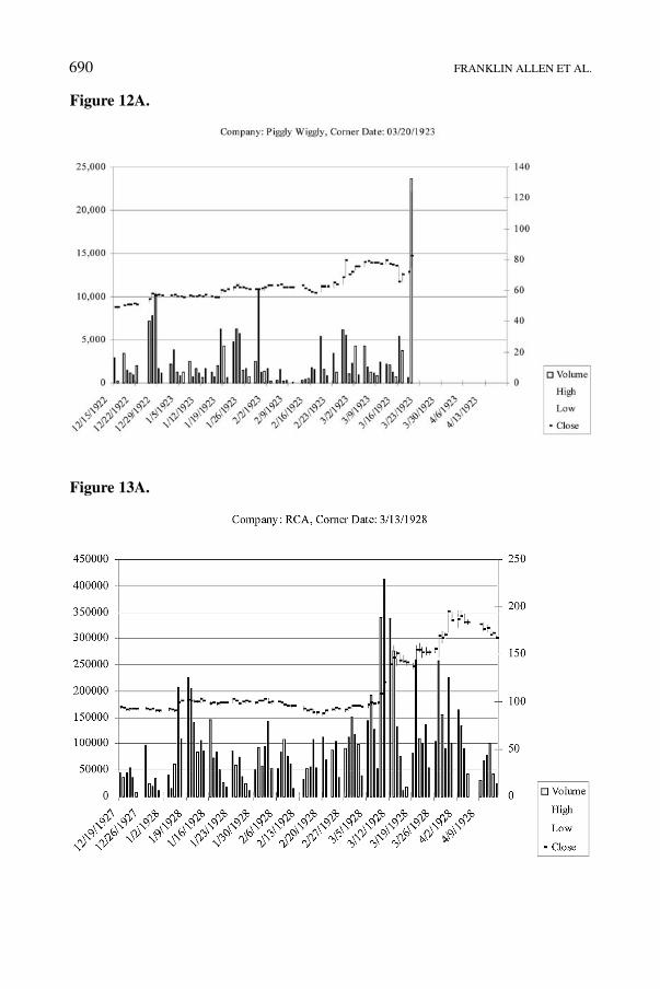
688 FRANKLIN ALLEN ET AL.
Figure 12A.
Figure 13A.
690

LARGE INVESTORS, PRICE MANIPULATION, AND LIMITS TO ARBITRAGE 689
Figure 14A.
References
Aggarwal, R. and Wu, G. (2006) Stock market manipulation, The Journal of Business 79, 1915–1953.Allen, F. and Gale, D. (1992) Stock price manipulation, Review of Financial Studies 5, 503–529.Allen, F. and Gorton, G. (1992) Stock price manipulation, market microstructure and asymmetric
information, European Economic Review 36, 624–630.Amihud, Y. (2002) Illiquidity and stock returns: Cross-section and time-series effects, Journal of
Financial Markets 5, 31–56.Bagnoli, M. and Lipman, B. (1996) Stock price manipulation through takeover bids, RAND Journal
of Economics 27, 124–147.Benabou, R. and Laroque, G. (1992) Using privileged information to manipulate markets: Insiders,
gurus and credibility, Quarterly Journal of Economics 105, 921–958.Brooks, J. (1969) Once in Golconda: A True Drama of Wall Street 1920–1938, Harper & Row, New
York.Chakraborty, A. and Yilmaz, B. (2004a), Informed manipulation, Journal of Economic Theory 114,
132–152.Chakraborty, A. and Yilmaz, B. (2004b) Manipulation in market order models, Journal of Financial
Markets 7, 187–206.Chancellor, E. (2000) Devil Take the Hindmost: A History of Financial Speculation, Plume Books,
New York.Cherian, J. A. and Jarrow, R. A. (1995) Market manipulation, in R. A. Jarrow, V. Maksimovic, and W.
T. Ziemba (eds.), North-Holland Handbooks of Operations Research and Management Science:Finance (Volume 9, chapter 9), Elsevier, New York, pp. 611–630.
Clews, H. (1888) Twenty Eight Years in Wall Street, Irving Publishing Co., New York.Flynn, J. T. (1934) Security Speculation: Its Economic Effects, Harcourt Brace, New York.
691
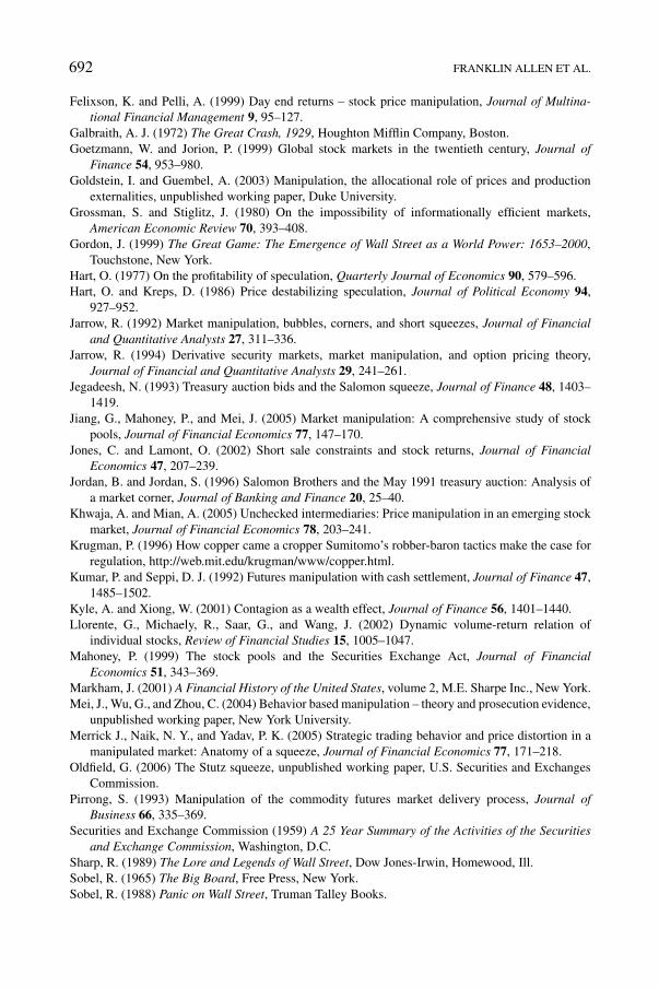
690 FRANKLIN ALLEN ET AL.
Felixson, K. and Pelli, A. (1999) Day end returns – stock price manipulation, Journal of Multina-tional Financial Management 9, 95–127.
Galbraith, A. J. (1972) The Great Crash, 1929, Houghton Mifflin Company, Boston.Goetzmann, W. and Jorion, P. (1999) Global stock markets in the twentieth century, Journal of
Finance 54, 953–980.Goldstein, I. and Guembel, A. (2003) Manipulation, the allocational role of prices and production
externalities, unpublished working paper, Duke University.Grossman, S. and Stiglitz, J. (1980) On the impossibility of informationally efficient markets,
American Economic Review 70, 393–408.Gordon, J. (1999) The Great Game: The Emergence of Wall Street as a World Power: 1653–2000,
Touchstone, New York.Hart, O. (1977) On the profitability of speculation, Quarterly Journal of Economics 90, 579–596.Hart, O. and Kreps, D. (1986) Price destabilizing speculation, Journal of Political Economy 94,
927–952.Jarrow, R. (1992) Market manipulation, bubbles, corners, and short squeezes, Journal of Financial
and Quantitative Analysts 27, 311–336.Jarrow, R. (1994) Derivative security markets, market manipulation, and option pricing theory,
Journal of Financial and Quantitative Analysts 29, 241–261.Jegadeesh, N. (1993) Treasury auction bids and the Salomon squeeze, Journal of Finance 48, 1403–
1419.Jiang, G., Mahoney, P., and Mei, J. (2005) Market manipulation: A comprehensive study of stock
pools, Journal of Financial Economics 77, 147–170.Jones, C. and Lamont, O. (2002) Short sale constraints and stock returns, Journal of Financial
Economics 47, 207–239.Jordan, B. and Jordan, S. (1996) Salomon Brothers and the May 1991 treasury auction: Analysis of
a market corner, Journal of Banking and Finance 20, 25–40.Khwaja, A. and Mian, A. (2005) Unchecked intermediaries: Price manipulation in an emerging stock
market, Journal of Financial Economics 78, 203–241.Krugman, P. (1996) How copper came a cropper Sumitomo’s robber-baron tactics make the case for
regulation, http://web.mit.edu/krugman/www/copper.html.Kumar, P. and Seppi, D. J. (1992) Futures manipulation with cash settlement, Journal of Finance 47,
1485–1502.Kyle, A. and Xiong, W. (2001) Contagion as a wealth effect, Journal of Finance 56, 1401–1440.Llorente, G., Michaely, R., Saar, G., and Wang, J. (2002) Dynamic volume-return relation of
individual stocks, Review of Financial Studies 15, 1005–1047.Mahoney, P. (1999) The stock pools and the Securities Exchange Act, Journal of Financial
Economics 51, 343–369.Markham, J. (2001) A Financial History of the United States, volume 2, M.E. Sharpe Inc., New York.Mei, J., Wu, G., and Zhou, C. (2004) Behavior based manipulation – theory and prosecution evidence,
unpublished working paper, New York University.Merrick J., Naik, N. Y., and Yadav, P. K. (2005) Strategic trading behavior and price distortion in a
manipulated market: Anatomy of a squeeze, Journal of Financial Economics 77, 171–218.Oldfield, G. (2006) The Stutz squeeze, unpublished working paper, U.S. Securities and Exchanges
Commission.Pirrong, S. (1993) Manipulation of the commodity futures market delivery process, Journal of
Business 66, 335–369.Securities and Exchange Commission (1959) A 25 Year Summary of the Activities of the Securities
and Exchange Commission, Washington, D.C.Sharp, R. (1989) The Lore and Legends of Wall Street, Dow Jones-Irwin, Homewood, Ill.Sobel, R. (1965) The Big Board, Free Press, New York.Sobel, R. (1988) Panic on Wall Street, Truman Talley Books.
692

LARGE INVESTORS, PRICE MANIPULATION, AND LIMITS TO ARBITRAGE 691
Stedman, E. C. (1905) The New York Stock Exchange; its History, its Contribution to NationalProsperity and its Relation to American Finance at the Outset of the Twentieth Century,Greenwood Press, New York.
Thomas, D. (1989) The Plungers and the Peacocks: An Update of the Classic History of the StockMarket, William Morrow and Company, Inc., New York.
Twentieth Century Fund (1935) Security Markets, H. Wolff, New York.Van Bommel, J. (2003) Rumors, Journal of Finance 58, 1499–1520.Vila, J. L. (1987) The role of information in the manipulation of futures markets, unpublished
working paper 87-26, CARESS, University of Pennsylvania.Vila, J. L. (1989) Simple games of market manipulation, Economics Letters 29, 21–26.Vitale, P. (2000) Speculative noise trading and manipulation in the foreign exchange market, Journal
of International Money and Finance 19, 689–712.Wycoff, R. (1968) Wall Street Ventures and Adventures, Greenwood Press, New York.Wyckoff, P. (1972) Wall Street and the Stock Market: A Chronology (1644–1971), Chilton Book
Company, Philadelphia.
693


![Image Manipulation with Perceptual Discriminators · image manipulation tasks both due to their ability to train on large amount of data [20,23,12] and due to natural image priors](https://static.fdocuments.in/doc/165x107/600985c8dc290005d5618bd5/image-manipulation-with-perceptual-discriminators-image-manipulation-tasks-both.jpg)