Large Investors: Implications for Equilibrium AssetReturns, Shock Absorption, and Liquidity

Matthew Pritsker∗

First version: August 31, 2001

This version: April 9, 2002

Abstract

The growing share of financial assets that are held and managed by a relativelysmall number of large institutional investors calls into question the traditional assetpricing paradigm of perfectly competive markets with small price-taking players. In thispaper, I relax the traditional price-taking assumption and instead present static anddynamic multi-asset, multi-large participant models of imperfect competition in riskyasset markets. Both model contain a fringe of small risk-averse investors who behavecompetitively, and a set of large risk-averse institutional investors who are Cournotcompetitors. The imperfect competition assumption implies large investors face anilliquidity cost when trying to rebalance their portfolios. In the static model, when allinvestors ignore this cost, asset prices satisfy the CAPM. When large investors insteadaccount for the effect that their trades have on prices, then in simple variants of thestatic model, prices inherit a two-factor structure—in which one factor is the marketportfolio, and the other is the endowment of assets held by institutional investors.When some institutions experience a shock in which they need to raise cash by sellingassets, then the cross-section of asset prices has a three factor structure and a non-zeroalpha which is related to institutional cash needs.

In a dynamic setting with full disclosure of trades and positions, investor with dif-ferent characteristics face different market liquidity conditions even when they proposethe same trades. This result suggests that when trades can potentially move prices,large participants have an incentive to hide the identity of the party who is behinda trade. The dynamic model is also used to examine the effect of news about somemarket participants potential future financial distress affects current asset prices.

Keywords: Strategic Investors, Contagion, Cournot CompetitionJEL Classification Numbers: F36, G14, G15, D82, and D84

∗Board of Governors of the Federal Reserve System. The views expressed in this paper are those of theauthor but not necessarily those of the Board of Governors of the Federal Reserve System, or other membersof its staff. Address correspondence to Matt Pritsker, The Federal Reserve Board, Mail Stop 91, WashingtonDC 20551. Matt may be reached by telephone at (202) 452-3534, or Fax: (202) 452-3819, or by email atmpritsker@frb.gov.

1 Introduction

An increasingly large share of financial assets are owned or managed by large institutional

investors. How does the presence of large investors in financial markets affect equilibrium

asset prices, liquidity, and the transmission of shocks across asset markets?

In this paper, I present 2 models of financial markets in order to shed light on these

questions. The first model is a an essentially static two-period model which only involves

a single period of trade. The second model is a multi-period extension of the first model.

The extension to multiple time periods makes it possible to examine the dynamics of the

market’s adjustment to shocks. It also allows for much richer strategic interaction than in

the two period setting.

The general modelling approach is designed to be consistent with the empirical observa-

tions that the orderflow of institutional investors is often large relative to the scale of some of

the markets in which they trade, and institutional investors follow trading strategies which

account for the effect that their orderflow has on asset prices [Chan and Lakonishok (1995)].

Both models contain large and small investors. Small investors behave competively by

taking asset prices as given. Each small investor is assumed to be infinitesimal relative to the

size of the market, and collective actions of the small investors is assumed to be represented

by a single non-infinitesimal competitive investor who takes prices as given. The competitive

investor will often be referred to as the competitive fringe. The large investors in both models

trade strategically by accounting for the effect that their trades have on asset prices.

In each period that markets are open, prices in all asset markets are determined by large

investors simultaneously choosing the amounts of assets they wish to buy or sell in each

asset market while taking the demand curve of fringe investors as given. The resulting set of

large investor trades is a subgame perfect Cournot-Nash equilibrium. The equilbrium trades

are the same as those which would result if each large participant chose its optimal trade

when faced with the residual demand curve that is determined by the demands of the fringe

investors and the optimal trades of the other large participants.

In both models, when investors are sufficiently similar, and all investors behave compet-

itively, equilibrium asset prices and holdings satisfy the Capital Asset Pricing Model. By

contrast, in the single period model, when large investors instead account for the effect that

their trades have on asset prices, then when large investors are sufficiently similar1, asset

prices have a two factor structure. The first factor is the market portfolio and the second

is large investors’ endowment of risky assets. The price of risk in the resulting factor model

1In the setting below, large investors will be sufficiently similar if they have the same absolute riskaversion.

1

will depend on market structure. In particular it depends on the number of large investors

in the market, their absolute risk aversion, and the size and risk aversion of investors in

the competitive fringe. In the multi-period model, the dynamics of asset prices are much

more complicated. I have not yet examined whether asset prices satisfy a factor model in a

multiperiod setting.

An important reason for studying the behavior of markets with large participants is to

understand the effect that large participants have on market liquidity, and on the propagation

of shocks through the financial system. This question of shock transmission is of special

interest in light of the problems during 1998 for LTCM, one large participant, and the

apparent drying up of liquidity in other markets. To study these issues, I solve for the effect

on equilibrium asset prices if some of the large participants in the model experience a shock

in which they have to raise cash by selling off some of their risky assets. Using the single-

period model, I show that equilbrium expected excess returns, after responding to the shock,

have a 3-factor structure with a non-zero alpha. The first factor is the market portfolio, the

second factor is the asset endowments of large participants who are not directly hit with the

shock, and the third factor is the endowment of those participants who are forced to sell

assets. By contrast, when all investors are small, shocks affect the prices of all assets, and

alpha’s are non-zero, but the market portfolio is the only priced factor.

I also examine the effect of cash shocks in a multiperiod setting. My preliminary analysis

indicates that the initial price effects of a cash shock, and the time it takes to recover from

the shock, depends on which participants are hit with the shock.

Because the response of asset prices to shocks depends on participants endowments, if

the shock is anticipated, or partially anticipated, then this should affect asset prices because

market participants should adjust their asset holdings to hedge against, or take advantage

of the anticipated shock. To examine the effects of news about shocks on asset prices, I solve

for the markets’ price response to news about future shocks. In particular, I examine the

effect on asset prices of news or rumors that a particular participant or group of participants

may need to sell off part of their portfolio due to financial distress. This type of news might

for example be interpreted as news that LTCM is encountering financial difficulty, and the

resulting price responses may indicate the types of price responses that might be expected

in such circumstances. Solving for the price response to news about possible future shocks

requires a multiperiod model. Therefore, I restrict my analysis of the effects of news to the

the multiperiod setting.

The model of strategic trading that I present below is related to the voluminous litera-

ture on liquidity in financial markets. In much of this literature the main sources of asset

illiquidity are exogenous transaction costs [Constantinides (1986), Heaton and Lucas (1996),

2

Vayanos (1998), Vayanos and Vila (1999), Huang (1999)], asymmetric information about

asset payoffs [Glosten and Milgrom (1985), Kyle (1985), Kyle (1989), Eisfeldt (2001)] or

market participants endowments [Cao and Lyons (1999), Vayanos (1999), Vayanos (2001,

forthcoming)], and imperfect competition in asset markets due to large traders [Linden-

berg(1979), Kyle (1985), Kyle (1989), Basak (1997), Cao and Lyons (1999), Vayanos (1999),

DeMarzo and Urosevic (2000), Vayanos (2001, forthcoming), and Kihlstrom (2001)] or a

need to search for counterparties [Duffie et. al., (2001)].2 Although less common, illiquidity

has also been modelled as resulting from Knightian uncertainty [Cherubini and Della Lunga

(2001, forthcoming), Routledge and Zin (2001)]; or as the outcome of optimal security design

[Boudoukh and Whitelaw (1993), DeMarzo and Duffie (1999)].

This paper is closest in spirit to the literature on models of imperfect competition in

securities markets through the interaction of large market participants. One strand of this

literature has modeled imperfect competition and illiquidity together or as a result of the

presence of asymmetric information. I have chosen to not allow information asymmetry here

in in order to exclusively focus on other sources of illiquidity. Therefore, in this paper, the

only source of illiquidity in this model is imperfect competition. It is important to emphasize

that the assumption of no information asymmetry is very strong; it implies that all market

participants share the same information set and hence know each others’ asset holdings at

all points in time. In fact, this setting might be viewed as being perfectly transparent.

The effect of this transparency on the behavior of asset prices in the multiperiod model is

striking; and it is at least a bit suggestive of potential difficulties with requiring transparency

in markets.

This paper is very closely related to models of imperfect competion in which asymmetric

information is not present [Lindenberg(1979), Basak (1997), Kihlstrom (2001)]. Lindenberg

(1979) models the behavior of many large investors trading many assets in a single period

mean-variance setting. The one period model presented here is essentially one particular

case of Lindenberg’s model. The new part of our analysis of the one-period model is the

effect of liquidity shocks on asset prices in this setting. Hence our one period model is only

a slight modification of that of Lindenberg. The more interesting part of our analysis is the

multiperiod model. Basak(1997) and Kihlstrom(2001) have previously modelled the optimal

behavior of a single strategic trader in multi-period and two-period settings respectively.

Basak solves for securities prices in a multiperiod multi-asset model when the single strategic

trader can commit to his future trading strategy. In a single asset setting Kihlstrom solves for

the optimal trading strategy and prices in economies with a large investor who can commit,

2Corsetti et. al. (2001) do not explicitly focus on liquidity, but their model, because it focuses on largeplayers, is related to the literature on liquidity.

3

and one who cannot.

In the multiperiod model considered here, I extend the framework of Lindenberg (1979)

and Kihlstrom (2001) to a setting with multiple time periods, multiple risky assets, and many

large investors who engage in Stackelberg-Cournot competition in each trading period. The

only equilibria that I focus on are equilibria where commitment to a trading strategy is not

possible. The extension of strategic trading models to allow for multiple large investors was

suggested in Basak (1997).

It is important to distinguish the approach taken here with papers in the liquidity lit-

erature which assume that market participants are competitive. When participants are

competitive, their individual trades do not move prices, hence, abstracting from exogenous

transaction costs, individual participants in these models are not concerned with the liquid-

ity of asset markets as measured by the price impact of their trades.3 The competitive fringe

of participants in this paper also do not care about asset liquidity, but the large investors do.

It is also important to distinguish between liquidity shocks, and asset liquidity. A liquidity

shock is not a shock to the liquidity of asset markets. Instead, in the liquidity literature,

the standard convention is that a liquidity shock is a shock to an individual investor which

forces the investor to sell (or buy) specific assets. Typically, it is assumed that an investor

hit with a negative liquidity shock must sell all of their financial assets. The liquidity shocks

that I will use in this paper depart slightly from the standard treatment of negative liquidity

shocks. More specifically, the only liquidity shocks that are considered are the cash-flow

shocks alluded to earlier. My choice of modelling liquidity shocks as cash flow shocks has

three advantages relative to the more standard approach. First, investors are probably un-

likely to receive shocks to sell particular assets. Instead, they are more likely to receive

a call for cash, and then choose how to meet the request for cash. Second, the standard

treatment of liquidity shocks assumes that which assets are sold is specified exogenously. By

contrast, participants, when hit with a cash flow shock in the current model, endogenously

choose optimal asset sales while accounting for the risk characteristics of their portfolio, and

the liquidity of markets in which they are selling. Finally, the typical modelling of liquidity

shocks assumes that the entire portfolio must be eliminated. My approach, by contrast,

allows one to examine how cash flow shocks of different sizes affect asset prices.

Some of my analysis below is related to the literature on optimal liquidation of a trader’s

position. These papers solve for the optimal trajectory of sales to liquidate a position through

time. The relationship between these papers and the model that I present in the next section

is that both models have a trader or traders who must reallocate assets to raise cash according

3When markets are competitive, liquidity is sometimes measured as the price movement associated witha mass of traders buying or selling.

4

to some optimality criterion. In addition, both approaches involve traders that face an asset

illiquidity problem because their trades move prices. The difference in the two approaches

is that the illiquidity of markets in the optimal liquidation framework is typically specified

exogenously. By contrast, in my approach the liquidity of the asset market depends on the

nature of the imperfect competition in asset markets.

The remainder of the paper consists of five sections. The next section presents the

two-period model of asset markets and illustrates how large participants’ who account for

the price impact of their trades alters the factor structure of expected returns. It also

examines how large participants alter market liquidity. Section 3 extends the basic one-

period model to examine how unanticipated liquidity shocks to large participants spread

across markets. Section 4 presents the multiperiod model and its implications for liquidity.

Section 5 examines how news which helps market participants anticipate future liquidity

shocks affects asset prices. Section 6 concludes.

2 The Basic Imperfect Competition Model

The basic model is a two-period endowment economy. Before trade begins in the first

period, market participants receive an endowment of risky and riskless securities. After

participants receive their endowments, trade takes place in period 1. In period 2 all assets

pay a liquidating dividend—the liquidating value of the assets—and then investors consume.

The economy contains N risky assets, and a single risk-free asset. The risk-free asset

in the economy is the numeraire; and it is assumed to be in perfectly elastic supply. Its

liquidation value in period two is 1, and its price in period one is also normalized to 1. The

liquidation value of the risky assets is denoted by the N × 1 vector v. It is assumed that v

is distributed multivariate normal with mean v, and variance-covariance matrix Ω:

v ∼ N (v,Ω) (1)

The economy is populated by a continuum of small price taking investors, and by M

large investors. The small investors are collectively referred to as the “competitive fringe”,

or the “fringe.” Each of the small investors is assumed to have CARA utility. Without loss

of generality the collective asset demands of the small investors are represented by those of a

single representative price-taking investor who has CARA utility with absolute risk aversion

Af .4 The fringe’s endowment of risk free assets is denoted qf and its endowment of risky

assets is denoted by the N-vector Qf .

4The f signifies that the investor with risk aversion Af represents the competive fringe.

5

Each of the large investors is assumed to be large enough relative to the size of the market

so that their orderflow moves prices. They are assumed to account for their effect on prices

when choosing their orderflow. Each of the large investors is assumed to have a CARA utility

function with absolute risk risk aversion A. The m’th large investor’s initial endowments of

riskless and risky assets are denoted by qm and the N-vector Qm, respectively.

The economy’s total endowment of risky assets in the economy is denoted by the N -vector

X. By definition X satisfies the equation:

X = Qf +

M∑m=1

Qm (2)

Similarly, large investors total endowment of risk-free assets is denoted by qM , and qM

satisfies:

qM =

M∑m=1

qm (3)

There are many ways to interpret the presence of large investors in the model. My

preferred interpretation is that the large investors represent the demands of many small

portfolios that are collectively managed by institutional investors such as mutual funds, or

pension funds. The reasons why some small investors choose to trade on their own as part of

the competitive fringe, while others turn their portfolios over to large institutional investors

is not currently modelled.

At time 1, after investors receive their endowments, a single round of trade takes place

between all investors in the model. At the time trade takes place, large investors know the

form of the fringe investors demand function for risky assets. The fringe’s demand function

specifies the prices that the fringe investors require to absorb all possible net trades with the

set of large investors. Knowing the form of this demand function, each large investor submits

an N-vector of market orders which specifies the amount of risky assets that the investor will

purchase of each asset. This vector is also be variously referred to as the investors net-trade

vector. Given the large investors market orders, equilibrium prices are those which clear the

market in the sense that the amount of assets which the fringe purchases is just equal to the

risky asset sales by the large investors.

Because any large investor can influence the net trade of all large investors, each large

investor has market power in the sense that he/she can influence the price that the investor

(and all other investors) pay when purchasing the asset.

6

2.1 Solving the Model

Solving the model requires two steps. In the first step, I solve for the demand curve of

the fringe investors, and then use this demand function to solve for equilibrium prices as a

function of the net trades of the large investors. The second step involves solving for the

trades of the large investors. In solving for the trades of the large investors, I assume that

the large investors play an N market cournot game; i.e. they simultaneously submit their

market orders in all markets. The set of orders constitute a Cournot-Nash equilibrium if

each large participant’s orderflow maximizes her expected utility of terminal wealth given

the orders of the other investors.

Demand Curve for the Competitive Fringe

Let ∆Qf denote the fringe investors net purchase of risky assets from large investors. Let

P denote the price paid for this orderflow. Given these assumptions, the fringe’s time 2

random wealth is given by

W f2 = (Qf + ∆Qf )

′v + qf −∆Q′fP. (4)

For P to be the equilibrium price, the fringe’s holdings of risky assets must be utility maxi-

mizing at price P . This implies that ∆Qf maximizes:

E− exp(−AfWf2 ). (5)

The equilibrium demand of the fringe at prices P is well known, and is given by the right

hand side of the equation below:

∆Qf = A−1f Ω−1(v − P )−Qf . (6)

The right hand side of the equation is the net trade vector of the fringe at prices P . Setting

this equal to the net trade vector of the large investors, and then solving for price vector P

produces the price schedule the fringe offers to absorb the large investors net trade vector.

More specifically, let ∆Qm denote the net amount of risky assets purchased by the m’th large

investor. Then, −∑Mm=1 ∆Qm denotes the net sales by large investors. Setting these sales

equal to the fringe investors net purchases and solving for P produces the price schedule

7

faced by large investors:

P = v − AfΩQf + AfΩM∑

m=1

∆Qm. (7)

The Large Investors Portfolio Problem

The large investors optimal portfolio choice in equilibrium needs to be solved for as part of

the overall equilibrium of a market game for the M large participants. I solve this game by

solving for each of the large players Cournot reaction functions, and then use the reaction

functions to solve for the Cournot-Nash equilibrium of the game.

The solution to the game requires a bit of notation. Let ∆Q−m denote the set of market

orders submitted by all large investors other than large investor m, and let P (∆Qm; ∆Q−m)

represent the price schedule which is faced by large investor m when he submits order ∆Qm

and the orders of the other large investors are held constant at ∆Q−m.5 Given this price

schedule, the time 2 random wealth of the m’th large investor is given by:

Wm2 (∆Qm, Qm, qm; ∆Q−m) = (Qm + ∆Qm)′v + qm −∆Q′

mP (∆Qm,∆Q−m). (8)

The expression for wealth on the left hand side of (8) makes explicit the dependence of

time 2 weath on the initial endowments of risky assets and riskfree assets (Qm and qm

respectively). For these state variables, investor m’s utility of wealth is function is denoted

by ψm[Wm2 (∆Qm, Qm, qm; ∆Q−m)] where

ψm[W 2m(∆Qm, Qm, qm; ∆Q−m)] = − exp[−AWm

2 (∆Qm, Qm, qm; ∆Q−m)] (9)

The reaction function for large participant m is the trade vector which maximizes her

expected utility of time 2 wealth given her endowment, and given ∆Q−m. Denote this

reaction function by ∆Q∗m(Qm, qm; ∆Q−m). By definition the reaction function satisfies the

equation:

∆Q∗m(Qm, qm; ∆Q−m) = max

∆Qm

Eψm[Wm2 (∆Qm, Qm, qm; ∆Q−m)] (10)

It is now straightforward to define equilibrium trade vectors which constitute a Cournot-

Nash equilibrium.

5Substituting for ∆Qm, and ∆Q−m in equation (7) produces this price schedule.

8

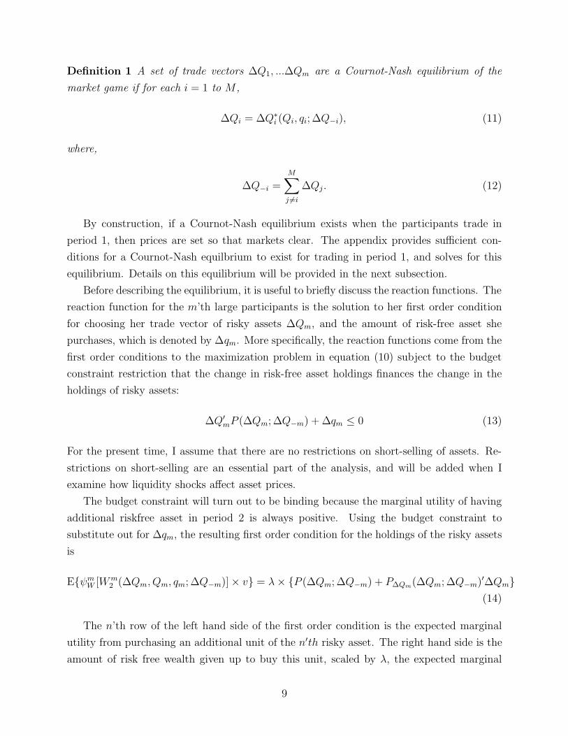
Definition 1 A set of trade vectors ∆Q1, ...∆Qm are a Cournot-Nash equilibrium of the

market game if for each i = 1 to M ,

∆Qi = ∆Q∗i (Qi, qi; ∆Q−i), (11)

where,

∆Q−i =

M∑j 6=i

∆Qj . (12)

By construction, if a Cournot-Nash equilibrium exists when the participants trade in

period 1, then prices are set so that markets clear. The appendix provides sufficient con-

ditions for a Cournot-Nash equilbrium to exist for trading in period 1, and solves for this

equilibrium. Details on this equilibrium will be provided in the next subsection.

Before describing the equilibrium, it is useful to briefly discuss the reaction functions. The

reaction function for the m’th large participants is the solution to her first order condition

for choosing her trade vector of risky assets ∆Qm, and the amount of risk-free asset she

purchases, which is denoted by ∆qm. More specifically, the reaction functions come from the

first order conditions to the maximization problem in equation (10) subject to the budget

constraint restriction that the change in risk-free asset holdings finances the change in the

holdings of risky assets:

∆Q′mP (∆Qm; ∆Q−m) + ∆qm ≤ 0 (13)

For the present time, I assume that there are no restrictions on short-selling of assets. Re-

strictions on short-selling are an essential part of the analysis, and will be added when I

examine how liquidity shocks affect asset prices.

The budget constraint will turn out to be binding because the marginal utility of having

additional riskfree asset in period 2 is always positive. Using the budget constraint to

substitute out for ∆qm, the resulting first order condition for the holdings of the risky assets

is

EψmW [Wm

2 (∆Qm, Qm, qm; ∆Q−m)]× v = λ× P (∆Qm; ∆Q−m) + P∆Qm(∆Qm; ∆Q−m)′∆Qm(14)

The n’th row of the left hand side of the first order condition is the expected marginal

utility from purchasing an additional unit of the n′th risky asset. The right hand side is the

amount of risk free wealth given up to buy this unit, scaled by λ, the expected marginal

9

utility of wealth. At an interior optimum the loss of utility from giving up risk-free wealth

must just offset the gain from purchasing additional risky asset. The amount of risk free

asset which is given up to buy an additional unit of risky asset n has two components, the

first component is the price of the risky asset. The second component is the effect that

buying an additional unit of asset n has on the price paid for inframarginal purchases of

asset n, and for the prices paid on inframarginal units of all other assets. In other words, the

strategic investors first order condition explicitly accounts for the effect that his orderflow

in each market has on the prices that he must pay in all other markets.

Solving for the reaction functions in the one period model is straightforward. The anal-

ysis shows that the m’th large investors reaction function in this framework satisfies the

relationship

∆Qm =AfQf − AQm

2Af + A− Af

2Af + A

M∑i6=m

∆Qi (15)

The reaction function has two interesting properties. The first is that an increase in Qm,

investor m’s endowment of the risky assets, has a less than one for one effect on ∆Qm, the

amount of risky assets that investor m wants to buy. The reason an increase in endowment

does not decrease desired purchases 1 for 1 is because selling off the increase in inventory

moves prices down and reduces revenue from selling. The second interesting property is that

the reaction functions are invariant to v and Ω. This invariance property is a special feature

of the one-period analysis; it is only satisfied in the last period of the multiperiod analysis.

2.2 Equilibrium Trades and Prices in the Basic Model

Equilibrium trades and prices can be found by using the reaction functions to solve for

∆Q1, . . .∆Qm which satisfy the system of equations given in definition 1. Using the reaction

function given in equation (15), the system of reaction function equations can be written as

2Af + A Af . . . Af

Af 2Af + A . . . Af

.... . .

...

Af . . . 2Af + A

⊗ IN

∆Q1

...

∆QM

=

AfQf − AQ1

...

AfQf − AQM

, (16)

where IN is the N ×N identity matrix.

This system clearly has a unique solution since the matrix inside square braces on the

left hand side is nonsingular.

10

Solving this system, the resulting set of equilibrium asset prices is given by:

P = v − Ω(Qf +∑M

m=1QM)

τf + (M + 1)τ− (τf/τ)ΩQf

τf + (M + 1)τ, (17)

where τ = (1/A) is the risk tolerance of each large investor, and τf = 1/Af is the risk

tolerance of the representative fringe investor.

The implications of this expression for price are examined in the next subsection.

2.3 Large Investors and the Cross-Section of Asset Prices

To examine the implications of large investors for the cross-section of equilibrium asset prices,

it is useful to first examine how prices would be set if all investors were price takers. The

behavior of prices under these circumstances is provided in the next proposition:

Proposition 1 If all investors in the model behave competively, then equilibrium asset prices

at time 1 are given by:

P = v − ΩX

τf +Mτ, (18)

where X is the outstanding number of shares of risky assets. In addition, the risky assets

expected excess returns over the riskless rate satisfy the Capital Asset Pricing Model.

Proof: This result is well known in the asset pricing literature (see for example the discussion

in Ingersoll [1987]). For completeness, I verify here that CAPM pricing holds in this setting.

Recall that when investors have CARA utility, the vector of assets’ excess return over the

riskless rate is measured in return per share instead or return per dollar, and is given by

v − RP where R is the gross riskless rate of return, which in this case is normalized to 1.

The excess return per share of the market portfolio is given by X ′(v − P ). This implies

that the mean and variance of the market’s excess return are respectively X ′(v − P ) and

X ′ΩX, and the vector of covariances of assets excess returns with the excess return of the

market portfolio is given by ΩX.

Manipulation of equation (18) shows that

v − P =ΩX

τf +Mτ, and,

X ′(v − P ) =X ′ΩXτf +Mτ

.

11

Dividing the first of these equations by the second and rearranging gives the CAPM pricing

equation:

(v − P ) = B(vm − Pm),

where B = ΩXX′ΩX

is an N × 1 stacked vector of the risky assets CAPM β’s, and (vm−Pm) =

X ′(v − P ) is the expected excess return on the market portfolio over the riskless rate. 2

It is useful to contrast the cross-sectional pricing of assets when all investors are price

takers with assets’ cross-sectional pricing when some of the investors take prices as given and

other investors behave strategically. The implications of this strategic behavior are provided

in the next proposition.

Proposition 2 [Lindenberg, 1979] For the basic asset pricing model with competitive and

strategic investors, the cross-section of excess returns is described by a 2-factor model. The

first factor is the market portfolio, and the second factor is the endowment of assets held by

large investors.

Proof: Using the definition of the total endowment (equation (2)) to substitute out for Qf

in the solution for equilibrium prices (equation (17)), and then simplifying shows that:

v − P =[1 + (τf/τ)]ΩX

τf + (M + 1)τ− (τf/τ)ΩQM

τf + (M + 1)τ, (19)

where QM =∑M

m=1Qm is the large participants endowment of risky assets.

From equation (19) it is clear that assets earn reward for risk based on their covariance

with the market portfolio (X), and based on their covariance with the initial endowments of

the large participants (QM). Q.E.D.

Proposition 2 is an important result because it establishes that large players who do not

take prices as given fundamentally change the way that risk is allocated in the market, and

hence alter the factor structure of asset returns, and the reward for risk. More importantly,

the proposition shows that the reward structure depends in part on who holds what assets.

The intuition for why who holds what matters is that large investors are more hesitant

to trade away from their initial endowments because the trading affects asset prices. This

hesitancy to trade leaves them holding more of their endowment than they would in a fully

competitive equilibrium (where everyone trades until they holds the market portfolio, as in

the CAPM). Because large investors are hesitant to fully trade out of their endowments, less

of the risk of these assets is borne by the market at large. Hence, these assets have higher

prices and lower expected returns, as shown by the negative reward for risk provided for QM

in equation (19).

12

2.4 Large Investors and Market Liquidity

One measure of the liquidity of the market is the price effect of changes in the outstanding

supply of assets. If markets are very liquid, the increase in asset supply will be absorbed with

only a small change in the price of the asset. Conversely, if markets are relatively illiquid, a

large change in price will be required to absorb the increase in supply.

To examine how changes in supply are absorbed, I consider increases in supply which

occur through increasing some participants endowments of risky assets. The resulting price

changes depend on how the change is risk from the increased endowment is spread among

investors. When there is imperfect competition in asset markets, how the risk is spread

depends on whose endowments are increased. I consider two polar cases. The first is that

the endowment of fringe investors is increased while that of large investors is held fixed. The

second is that the endowment of large investors is increased while that of the fringe investors

is held fixed.

To increase the fringe’s supply of risky assets, while holding the endowment of large

investors fixed involves increasing X while fixing Qm. From equation (19), the increase in

assets excess returns due to this increase in the fringe’s endowment is given by:

∂(v − P )

∂(Fringe Supply)=

[1 + (τf/τ)]Ω

τf + (M + 1)τ. (20)

Similarly, to increase large investors’ supply (endowment) of risky assets holding the

endowment of fringe investors fixed involves increasing X and Qm by the same amounts.

From equation (19), the increase in assets excess returns due to this change is given by:

∂(v − P )

∂(Large Supply)=

Ω

τf + (M + 1)τ(21)

It is useful to contrast the effects of these supply changes with the effect of a change in

asset supply when all market participants are competitive price takers. From equation (18),

the price effect of this supply change is given by

∂(v − P )

∂X

∣∣∣∣Comp. Mkts

=Ω

τf +Mτ(22)

An examination of the price effects of these supply changes show that all are equal to the

product of Ω multiplied by a scalar. Following the terminology in Kyle and Xiong (2001), I

will refer to this scalar as a magnification factor. It is the relative size of these magnification

factors which determine the relative liquidity of asset markets with perfect and imperfect

13

competition. Let ψf , ψlg and ψcomp denote the magnification factors in equations (20), (21),

and (22) respectively.

The relationship between the magnification factors in the imperfectly competitive and

competitive markets is given in the following proposition:

14

Proposition 3 The magnification factors for liquidity satisfy the following properties:

1.

limM−>∞

ψf

ψcomp

= 1 +τfτ.

2.

ψlg < ψcomp.

3.

limM−>∞

ψlg

ψcomp= 1.

The proposition has two important results. The first is that shocks to the endowments

of fringe participants have a much larger effect on asset prices when markets are imperfectly

competitive than when they are perfectly competitive. The intuition for why is simple.

When the fringe receives an endowment shock, and responds by selling assets, the price

effect depends on other participants willingness to buy. When markets are imperfectly

competitive, large investors will be relatively less willing to buy in response to the asset sales

because they know by purchasing less aggressively, they will get a lower price.

The second result is that increases in the endowments of large participants have less effect

on market prices than increases in endowments when markets are competitive. The reasons

why are similar: large participants are less willing than competitive participants to attempt

to unload a position when they experience an endowment shock because they take the price

impact of their trades into account.

3 Large Participants and Liquidity Shocks

In this section of the paper, I examine the effect that liquidity shocks have on equilibrium

asset returns. Two types of liquidity shocks are considered. The first type are liquidity

shocks which force investors to sell assets in order to make a cash payment of L dollars. The

destination of these payments, and the source of the shocks are not explicitly modelled. The

second type are shocks which cause an investor to liquidate their entire portfolio of risky

assets. The price response to the second type of liquidity shocks are primarily examined

because they are similar to the types of shocks considered in the liquidity literature.

15

3.1 The Perfect Competition Benchmark

It is useful to begin by examining the effect that the first type of liquidity shocks have on

equilibrium asset prices when all investors behave competitively. To remain consistent with

the imperfect competition model, I assume that there M + 1 investors who take prices as

given and have CARA utility. Here, I increase generality slightly by allowing the investors to

have differing absolute risk aversions Am, m = 1, . . .M+1. Them’th investor has endowment

qm and Qm of risky and risk free asset respectively, and chooses ∆Qm and ∆qm to maximize

Eψm[W 2m(∆Qm,∆qm, Qm, qm)]. (23)

subject to constraints which depend on whether the investor receives a liquidity shock.

When the investor is hit with a liquidity shock of the first type, the constraints take the

form:

qm + ∆qm ≥ 0, (24)

∆qm + ∆Q′mP ≤ −L. (25)

The first constraint (equation (24)) is referred to as the risk-free borrowing constraint because

it limits the amount of riskfree asset which can be sold short. For simplicity, the limit is set

at zero. The second constraint is referred to as the budget constraint; it requires that the

cash L is raised through sales of riskfree and risky assets. The maximization problem and

the constraints together imply that investors who are hit with a liquidity shock choose to

sell assets in a utility maximizing fashion.

Investors who are not hit with a liquidity shock choose ∆Qm and ∆qm to maximize their

expected utility (equations (23)) subject to:

∆qm + ∆Q′mP ≤ 0, (26)

where equation (26) is the standard budget constraint requirement that the net expenditure

on risky and risk-free assets is 0.

The consequences of type I liquidity shocks for the cross-section of asset prices in this

framework is given in the following proposition:

Proposition 4 In the competitive economy described in section 3.1, when some investors

are hit with a liquidity shock which requires them to raise L of cash, when all investors are

price takers, and when investors who are hit with a liquidity shock can raise the necessary

16

funds by selling assets, then equilibrium asset excess returns over the risk rate have the form

v − p = k1v + k2ΩX, (27)

where k1 and k2 are greater than zero, and

k1 =

∑M+1m=1

cm−1Am∑M+1

m=1cm

Am

, k2 =M+1∑m=1

cmAm

, (28)

and where cm = 1 for investors that are not hit with a liquidity shock and cm is greater than

1 for investors that are hit with a liquidity shock whose size exceeds the investor’s holdings

of riskfree assets.

Proof: See the appendix.

The main qualifier in the proposition is that investors are assumed to be able to fully

satisfy their liquidity shock. Since prices are a linear function of investors trades, there may

be circumstances where additional selling cannot generate enough revenue to meet the needs.

For the purposes of this proposition, I assume that this cannot happen. When investors can

raise enough revenue by selling assets, then the form of the proposition is correct.

To further interpret the proposition, note that when all of the the cm are all equal to

1 in the proposition, then the no short sales of the riskfree asset constraint is not binding.

Under these circumstances, the CAPM holds. However, when some of the cm are greater

than 1, then the no short-sales constraint (equation (24)) is binding for some investors. As a

result, the investors that need to raise cash need to sell risky assets. This binding constraint

has two effects on the cross-section of returns. First, all assets acquire a non-zero alpha,

and the size of the non-zero alpha is proportional to v, the assets expected terminal value.

The second effect is that the reward for bearing market risk (which is proportional to k2)

increases. The intuition for these results comes from noting that when some investors need

to sell assets to raise cash, the Euler conditions which are typically used to derive the CAPM

pricing equations are not satisfied, and hence risky assets earn liquidity premia.6

6To illustrate how the Euler conditions are violated, let γ and λ denote the Lagrange multipliers for theno short-selling constraint (equation (24)) and for the budget constraint (equation (25)), and let U(.) denotethe investor’s utility of final wealth. The first order conditions for a constrained investors choice of riskfreeand risky assets imply:

0 = E[U ′(.)]− λ + γ

0 = E[U ′(.)v − λp.

Because both constraints are binding, λ and γ are not equal to zero.Combining the first order conditions while recalling that vm = X ′v, pm = X ′p, and the gross-risk free rate

17

By contrast, if liquidity shocks simply force investors to liquidate their portfolios of risky

assets, then after the shock the risky assets will be priced as if the CAPM is satisfied. This

result is obvious because the forced liquidation only has the effect of changing the number of

investors, while leaving the supply of risky assets the same. Since the CAPM holds in this

setting for any numbers of competitive investors, it will hold when some of these investors

are eliminated. For completeness, this result is restated below:

Corollary 1 In the economy described by equations , when some investors are hit with a

liquidity shock which requires them to sell all of their asset holdings, and when all investors

are price takers, then equilibrium asset excess returns over the risk rate satisfy the CAPM,

i.e.

v − p = k3ΩX,

where k3 > 0.

The next section revisits these results when the market has both large and small market

participants.

3.2 The effect of large participants

In this section of the paper, I consider the situation when some large participants are hit with

liquidity shocks. The first type of shock I consider are cash flow shocks which cause investors

to alter their risky asset portfolio in order to raise L dollars in cash. A large participant m

who is hit with this type of shock before trading occurs at time 1, chooses his trade vector

of risky assets ∆Qm, and riskfree assets ∆qm to maximize:

Eψm[W 2m(∆Qm,∆qm, Qm, qm; ∆Q−m)] (29)

is 1, shows that:

E[U ′(.)(vm − pm) = γpm

6= 0.

This is a violation of the standard CAPM Euler condition that

E[U ′(.)(vm − pm) = 0.

The source of the violation is that γ, the shadow value of relaxing the constraint on short sales of bonds isnonzero.

Related research shows that limited short-selling is necessary to generate liquidity premia when thereare two riskfree assets with different amounts of liquidity [Krishnamurthy (2001), Boudoukh and Whitelaw(1993)].

18

subject to the constraints that:

qm + ∆qm ≥ 0 (30)

∆qm + ∆Q′mP (∆Qm; ∆Q−m) ≤ −L (31)

The constraints are nearly identical to the constraints that I imposed when asset mar-

kets are competitive. The difference is that prices in asset markets are now written as

P (∆Qm; ∆Q−m), and hence in the constraints each participant accounts for the effect that

his trades have on equilibrium asset prices.

The equilibrium with large participants is solved for by deriving participants reaction

functions, and then using the reaction functions to solve for the Cournot-Nash Equilibrium.

The conditions under which I solve for the equilibrium are somewhat less general than in

section 3.1, where all investors behaved competively. More specifically, in this section, I

assume that there are M large investors with CARA utility, and absolute risk aversion

A, and there is 1 representative competitive investor with absolute risk aversion Af . It is

assumed that K of the large participants are hit with a cash flow shock which requires each

of them to raise L of cash. Under this scenario, the effect of these cash flow shocks on

expected excess returns is provided in the next proposition:

Proposition 5 Under the conditions assumed in section 3.2, when K large market partic-

ipants experience a liquidity shock of identical size L, and when the large participants can

raise the required cash, then equilibrium expected excess returns have a 3-factor structure with

a non-zero alpha. The first factor is the market portfolio, the second factor is the endowment

of assets held by large participants who do not experience the shock, while the third factor is

the endowment of assets held by large participants who do experience the shock:

v − p = θ0v + θ1ΩXm + θ2ΩQns + θ3ΩQs, (32)

where Xm is the market portfolio, Qns is the net endowment of large participants that do not

experience a shock, and Qs denotes the endowment of the large participants that do experience

a shock.

Proof: See the appendix.

The proposition shows that assets earn a risk premium for covariance with the market

portfolio, the endowments of large investors who are hit with a liquidity shock, and the

endowments of large investors that are not hit with the shock. The cross-sectional structure

of asset prices in proposition 5 shares aspects of the results from propositions 2 and 4. The

19

cross-section of expected returns here and in proposition 2 both have a factor structure. The

cross-section of expected returns here and in proposition 4 also has a non-zero alpha which

is related to risky assets contributions to meeting some participants liquidity needs.

The most important implication of the proposition is that it shows that large participants

endowments of risky assets before a shock occurs have important effects on how shocks

propagate across markets, and how they are absorbed. This will be further explored in the

context of the multiperiod model.

4 The Multiperiod Model

Our multiperiod model is an extension of the work of Kihlstrom (2001). Recall from the

introduction that Kihlstrom’s (2001) model has a single risky asset and a single large trader

who takes the markets demand curve as given when solving for his optimal trading strategy.

Kihlstrom shows that in this set-up when there are two trading periods, shares of stock are

analogous to durable goods; and therefore the large trader faces a similar problem to Coase’s

durable goods monopolist: his optimal sales strategy in the future competes with his current

strategy. As a result, the large trader, competing against his own future self provides a price

path which results in lower prices than if he could commit to a pricing strategy in advance.

The framework that I present here is a multi-period, multi-asset, multi-large participant

extension of Kihlstrom’s model. The model contains M participants indexed m = 1, . . .M ,

N assets, and T time periods. The model is solved by backwards induction under the

assumption that T is finite.

4.1 Participants

All participants in the model choose their asset holdings to maximize their discounted ex-

pected future utility of consumption:

Um(Cm(1), . . . , Cm(t)) =

T∑t=1

δtUm(Cm(t)) (33)

where Cm(t) represents time t consumption for the m’th investor, δt represents investors

discount factors (assumed common across investors for now), and investors have CARA

utility of per period consumption with coefficient of risk aversion Am:

U(Cm(t)) = −e−AmCm(t) m = 1, . . .M (34)

20

The first participant (m = 1) is the fringe investor. The fringe takes prices as given when

choosing its demand for assets. The other investors choose their asset demands given the

fringe’s demand curve.

4.2 The Assets

The economy contains a single riskless asset in perfectly elastic supply which pays gross

rate of return r > 1 each period. I interpret the riskless asset as a money market account;

consequently assets in this account are cash; and are hence perfectly liquid. The economy

also contains N risky assets with fixed supply X. Unless explicitly stated otherwise, I assume

that during trading periods, investors can take unlimited long or short positions in the risky

or riskless assets, but the sum of total asset holdings across investors is restricted to equal

the outstanding supply of assets in the economy. The payoffs of the risky assets come in the

form of perfectly liquid cash dividends. In each period t the risky assets pay dividend D(t)

which has distribution

D(t) ∼ i.i.d. N (D,Ω) (35)

The assumption that dividends are i.i.d. is made for simplicity, and can be relaxed in future

extensions of this model.

4.3 Timing

At each time t < T each investor m enters the period with risky asset holdings Qm(t), and

riskless asset holdings qm(t), where qm(t) is inclusive of all interest earned from the end of

period t−1 to the beginning of period t. After entering the period investors receive dividends

on their holdings of risky assets. Thus, total dividends paid out to investor m in period t

are equal to Qm(t)′D(t). After investors receive their dividends, then they choose how much

to consume in period t and they trade risky and riskless assets. The price of risky assets in

terms of riskless assets in period t is denoted P (t). The change in investor m’s holdings of

risky assets (the amount of net purchases during trade) in period t is denoted ∆Qm(t), and

the change in her riskless asset holdings is denoted ∆qm(t). Consumption, and changes in

asset holdings for each investor must satisfy the budget constraint:

Cm(t) + ∆Qm(t)′P (t) + ∆qm(t) ≤ Qm(t)′D(t). (36)

21

This budget constraint is entirely standard and simply requires that expenditure on con-

sumption in period t which is in excess of period t dividend income must be financed by

sales of risky and riskfree assets.

After trades and consumption have been chosen, the new holdings of risky and risk-free

assets are carried into the next period. Thus, risky assets in period t+ 1 satisfy:

Qm(t+ 1) = Qm(t) + ∆Qm(t). (37)

Riskless assets that are available at the end of period t grow at rate r between time periods.

Thus,

qm(t+ 1) = r(qm(t) + ∆qm(t)) (38)

At time T , no trades take place. Instead investors receive dividends on their risky asset

holdings, and then consume their dividends and holdings of riskless assets.

4.4 Solving the Model

The complete solution for the model is provided in the appendix. The main solution tech-

nique is dynamic programming and backwards induction. First, I conjecture that the relevant

state variables at each time period is the entire vector of all investors risky asset holdings.

Given this state vector, there are four main steps in the induction. First, for a given state

vector, I solve for the fringe’s demand function for risky assets in the final period of trade.

Second, given this demand function, I solve for large participants equilibrium asset trades in

the last period, when taking the fringes demand function as given. Third, given the equilib-

rium trades, I solve for participants optimal consumption choices in the last trading period,

and then use the result to solve for each investors value function of entering the last period

of trade for a given set of state variables.

Given the value function of entering the last period with a given set of state variables,

it is possible to then step back one period in time and derive the fringe investors demand

for risky assets in the second to last trading period as a function of the state vector and

of proposed trades by the large investors. From this point, the model is solved by again

following steps two through four, then stepping back another period in time, and so on, until

time period 1.

22

Fringe’s Demand Curve

The form of the fringe’s demand curve in each time period deserves additional comment.

In the appendix, I show that at each time t, conditional on dividends in period t, the

demand curve provided by the fringe comes from the first order condition to the maximization

problem:

maxC1(t),∆Q1(t),∆q1(t)

−e−A1C1(t) + δEtV1(Q(t) + ∆Q(t), q1(t) + ∆q1(t), t+ 1) (39)

subject to the budget constraint,

C1(t) + ∆Q1(t)′P (t) + ∆q1(t) ≤ Q1(t)

′D(t),

where Q(t) = stackMm=1Qm(t) and ∆Q(t) = stackM

m=1∆Qm(t), are the stacked vectors of

investors risky asset holdings and trades at time t, and where the consistency condition

∆Q1(t) = −M∑

m=2

∆Qm(t)

is satisfied.

The fringe’s demand function is a bit unconventional, but it is intuitive; basically the

demand function is the solution to the question given a set of proposed trades ∆Q2, . . .∆QM

by the large investors, what price P is required so that the fringe absorbs the net trades of the

large investors. An important feature of this particular demand curve is that it is conditional

on the distribution of risky asset holdings across the investors, and on the distribution of

net trades.7

The fringe demand curve’s explicit conditioning on the distribution of assets across in-

vestors when forming its demands is an important departure from the fringe’s demand curve

in the static model that I presented earlier. The reason for the difference is that the fringe’s

demand for risky assets in the static model only depends on the fringe’s consumption in

the final period. Since the fringe’s final period consumption depends only on its own asset

holdings, there is not a strategic element to the fringe’s demand for risky assets in the final

period. By contrast, in the multi-period model, in all but the last trading period, the fringe

7Because of my assumption that investors have CARA utility, and that there are no restrictions on short-selling or borrowing, investors demands for risky assets do not depend on the distribution of risk-free assets.However, when a participant is hit with a liquidity shock, I assume that the participant who is hit with theshock cannot borrow cash to pay off his obligations. Under those circumstances, that investors holdings ofrisk-free assets is an important state variable to all investors.

23

cares about the future distribution of risky asset holdings among investors, since this af-

fects future equilibrium trades and prices. As a consequence, the fringe’s demand explicitly

conditions on the equilibrium trades of each large investor.

Investors Value Functions

As noted above, the relevant state variable for solving for investors optimal trades is the

vector of all investors holdings of risky assets. Hence, when there are M investors, and N

assets, the dimension of the state space (MN) is fairly high. Typically, a dynamic model

with a high dimensional state space would be difficut to solve unless there are simplifying

assumptions. The simplifying assumptions here are that investors have maximize time-

separable CARA utility of consumption, and assets’ dividends are normally distributed, and

i.i.d. through time. Because of these assumptions risky asset demands are a linear function

of the state variables, and investors value functions at each time t are exponential linear

quadratic functions of the state variables. For example, for investor m, the value function

has form:

Vm(Q(t), qm(t), t) = −km(t)e−Am(t)Q(t)′ vm(t)+.5Am(t)2Q(t)′θm(t)Q(t)−Am(t)rqm(t) (40)

The parameters of investor m’s value function at time t are Am(t), vm(t), and θm(t).

Each parameter is the solution of a set of nonlinear Riccati difference equations. Because

of the simplicity of numerically solving the Riccati equations, it is possible to solve for the

behavior of asset prices in the dynamic model even when the number of investors and time

periods is large. A note of caution is required, however, because for some choices of the

risk aversion parameters (not the ones used below) the numerical solutions of the Riccati

equations are explosive. Further investigation of the numerical stability of the solution is

warranted before reaching any strong conclusions.

First and Second Order Conditions

Recall that in each time period, an intermediate step in solving for investors value functions

involves solving for large investors equilibrium trades given the competitive fringe’s demand

curve. The equilibrium demand curve comes from the first order condition of the competi-

tive fringe. Large investors equilibrium trades are found using investors reaction functions,

which also come from first order conditions for each investors optimal trades. These first

order conditions are sufficient to solve for investors optimal trades provided that each in-

vestors objective functions are strictly concave functions of their own trades when holding

the trades of other investors fixed. I have not yet established necessary and sufficient con-

24

ditions on investors absolute risk aversion, and on the distribution of dividends to establish

when investors objective functions are strictly concave functions of their trades. However, in

all of my analysis to date, I have numerically verified that all investors value functions are

concave in their own trades at each time period.8

4.5 Liquidity in the Multiperiod Model

A standard measure of liquidity which is used in the market microstructure is the price

impact associated with sales of an additional unit of risky assets. This notion of liquidity

is not wholly satisfying in a dynamic model of the type considered here because positing

that an investor sells additional units of risky assets is tantamount to assuming that the

investor follows a suboptimal strategy. Such behavior is essentially outside of my current

modelling framework because the model solution is based on all investors following their

optimal strategies given those followed by others. To study liquidity in the current model, I

primarily examine how changes in investors initial endowments affects the path of prices and

investors asset holdings. When there is illiquidity (i.e. when investors are not price takers)

then the price response will depend on which participant receives the endowment shock, and

on market liquidity conditions as measured by the demand curve faced by large investors,

and on the investors reaction functions.

To begin studying liquidity, it is useful to examine the fringe’s equilibrium demand curve,

which is the demand curve faced by large investors. One indicator of the liquidity conditions

that are faced by investors is the slope of this demand curve.

In period T − 1, the last trading period of the model, the demand curve of the fringe

investor has a very simple form:

P (t− 1) =1

r

(D − A1ΩQ1 + A1Ω

M∑m=2

∆Qm

)

=1

r

(D − A1ΩX + A1Ω

M∑m=2

(Qm + ∆Qm)

).

A notable feature of this demand curve is that, for all large investors m, the slope of the

demand curve relative to each large investors orderflow is the same and is equal to A1Ω. In

earlier periods, the demand curve has a similar, but slightly different form:

8In each time period, verification of global concavity only involves checking whether, for each investor,a particular matrix is negative definite. In all cases that I have examined, the relevant matrices have beennegative definite in every time period.

25

P (t− 1) =1

r(α1(t)− A1(t)βX(t)X +

M∑m=2

βm(t)(Qm + ∆Qm)), (41)

where βm(t) is the slope of the demand curve with respect to ∆Qm at time t.9 The intercept

at time t is given by α1(t)− βX(t)X. When the large investors asset holdings are zero, the

intercept of the demand curve measures the fringe’s marginal value of risky versus riskfree

assets. The notable feature of this demand curve is that its slope is potentially different for

the trades of different large investors. This means that in periods prior to the last period of

trade, the fringe’s demand curve appears to offer different amounts of liquidity to different

large investors. This result is not quite as surprising as it sounds. Equilibrium prices in the

model represents the relative marginal value of risky and riskless asset holdings to the fringe.

When the distribution of risky assets across investors affects the strategic environment going

forward (as it does in every period except period T − 1), it is not surprising that the fringe’s

marginal valuations move by different amounts depending on who is doing the purchasing

from the fringe. This is borne out by the simulation analysis that follows.

4.6 Simulation Analysis of the Multiperiod Model

To illustrate the properties of the multiperiod model, I simulated the behavior of the model

for various values of the parameters of the model. The parameters were chosen to ensure

that the prices of all risky assets are positive in all time periods.10

The evolution of asset prices and trades is considered over 5 time periods in a framework

with a single risky asset, one competitive investor (investor 1), and 5 large investors. Divi-

dends are distributed normally with mean 5 and variance 1 in each period. Two choices are

considered for investors risk aversion. The first is that the competitive fringe and all large

investors have the same risk aversion. When all investors have the same risk aversion, the

model is relatively uninteresting. Hence, I focus most of my attention on a second case in

which each of the large investors have different risk aversion. This second case is my baseline

(see Table 2).

To begin the analysis, I examine how prices and trades evolve when all investors begin

with the same asset holdings and all investors have the same absolute risk aversion. Two

9In the appendix, I refer to the matrix [β2(t), β3(t), . . . , βM (t)] as βQB (t).10Although prices can be negative in this model because there is not limited liability, the possibility of

negative prices can lead to very unrealistic behavior in the presence of liquidity shocks. One example ofhow negative prices lead to perverse results occurs because an investor might respond to a liquidity shockby purchasing assets that have negative prices. This action raises money to pay for the shock, and drivesthe price of assets upward.

26

properties of this setting are worth noting. The first is that investors in do not alter their

risky asset holdings through time (Table 1, Panel C). This no-trade property occurs because

investors initial asset holdings are pareto optimal (hence there are no gains from trade)

and because the model satisfies the other conditions of the No-Trade Theorem of Milgrom

and Stokey (1982).11 It follows that pareto-optimal asset holdings are a steady state of the

model. The second property is that the risky asset’s liquidity in the model decreases through

time when liquidity is measured using the slope of the fringe’s supply curve (Table 1, Panel

B).12 It is important to emphasize that the slope of the fringe’s supply curve is not a fully

adequate measure of liquidity because the price effect of asset sales depends not just on

the fringe’s behavior, but also on other large investors willingness to buy when other large

investors are selling. One measure of this willingness to buy is the slope of large investors

reaction functions. By this measure (not shown), liquidity also decreases through time. I

do not currently have intuition to explain why liquidity decreases through time in this case.

The models other properties in this setting are in accord with intuition. As dividends are

paid out, and asset lives shorten, the price of the risky asset declines. For similar reasons,

the intercept of the fringe’s demand curve declines through time.13

To further examine the properties of the model, it is useful to allow investors to differ in

their absolute risk aversion. I consider a setting in which the representative fringe investor

has absolute risk aversion 1; the large investors’ absolute risk aversion ranges from 1 to 5;

and investors initial asset allocations are chosen to be pareto-optimal (Table 2, Panel A).

This variant of the model (whether considered for 5 periods, or longer) is referred to as the

baseline model.

The striking feature of the baseline model is the liquidity conditions. Two features of

liquidity in the model are worth noting. First, and most important, liquidity, as measured

using the slope of the fringe’s supply curve, is increasing in investors risk aversion. More

specifically, if one of two large investors were to purchase the same number of shares of risky

asset from the fringe, then prices will rise by more when the large investor with the lower

risk aversion is purchasing from the fringe (Table 2, Panel B). As noted above, an additional

indicator of liquidity is the slope of large investors reaction functions. Inspection of this

indicator (not shown) produces similar results: large investors are more willing to absorb

sales by other large investors when relatively more risk averse investors are selling. Thus, in-

terestingly, my results suggest that large investors with low risk aversion receive less liquidity

in the market. I have not yet fully explored the implications of my findings on differences

11I thank Peter DeMarzo for pointing out this property of the model.12A steeper supply curve means less liquidity.13Although the intercept is below zero in time periods 4 and 5, because the fringe does not hold all of the

risky assets during these time periods, equilibrium prices are positive.

27

in liquidity for different investors, but at a minimum it suggests that large investors have

incentives to hide their positions and trades because knowledge of those positions by other

investors can adversely affect an investor’s strategic position. It is important to emphasize

that there is no private information about asset values in the model. Instead, here it appears

that knowledge of an investors position is valuable because it affects the strategic equilib-

rium. Hence, when investors are large, asset positions themselves become information that

some investors may want to keep private.14

The second interesting feature of the liquidity conditions in the baseline model is that

liquidity, as measured by the slope of the fringe’s supply function, increases through time

between period 1 to period 4, but then liquidity decreases in period 5. By contrast, when all

investors had the same risk aversion, liquidity, as measured by the slope of the fringe’s supply

function, decreased through time (Table 1, Panel B). When the time pattern of liquidity is

examined using reaction functions, it turns out that large investors provide less liquidity to

each other through time. Hence, in this case, the two sets of liquidity indicators considered

together do not provide a coherent picture for whether liquidity is increasing or decreasing

through time.

To further examine liquidity, I study how endowment shocks, and cash flow shocks affect

the pattern of equilibrium risky asset holdings and asset prices. The analysis of these prices

is an extension of my examination of price responses to these types of shocks in the static

two-period model (see proposition 3 and section 5).

Endowment shocks

Recall that when investors have CARA utility, take prices as given, and face no constraints

on borrowing or short-sales, then the distribution of endowments across investors does not

affect asset prices. However, when markets are not perfectly liquid, in the sense that investors

trades move prices, then the analysis of the static model established that which investors

receive shocks affects equilibrium prices. The analysis in this subsection expands the earlier

analysis to examine the dynamic effects of endowment shocks on equilibrium prices and asset

holdings when markets are not perfectly liquid.15 For purposes of comparison, I shock the

endowments of the competitive fringe, and of large investors 2 and 6. Comparing the effects

of shocking the fringe and large investor 2, both of which have the same risk aversion),

allows me to examine how differences in price-taking behavior affect equilibrium prices and

trades. Similarly, comparing how investors 2 and 6, which have low and high risk aversion

14Solving for asset prices when investors positions are private information is likely to be very challenging,so I leave it for the future.

15I do not examine the effect of endowment shocks on the slope of the fringe’s demand curve since theslope of the fringe’s demand curve is not affected by endowment shocks.

28

respectively respectively, respond to the shock, allows me to examine the role of risk aversion

in the response to the shock.

When comparing the responses to the shock, several facts emerge. First, when compared

with the path of baseline asset holdings, the fringe’s asset holdings in response to its 1 share

shock at time 0 involve owning 0.4416 shares more than baseline one period after the shock,

and decline to owning 0.3091 shares above baseline after the final period of trade (Table 3,

Panel C). By contrast, when investor 2 is shocked instead, his equilibrium asset holdings are

0.7959 shares above baseline at time period 1, and fall to 0.3605 shares above baseline at

time period 5 (Table 4, Panel C). Comparing both of these results suggests that all else equal

price-taking investors sell more in response to an endowment shock than do large investors

who account for the impact of their trades on prices. As a result of the difference in investor

behaviors, the price paths in response to the two shocks are different. When the competitive

fringe receives an endowment shock the initial price effect relative to baseline is more than

thirty percent larger than when investor 2 is shocked. Moreover, prices when investor 2 is

shocked recover more quickly toward baseline prices than they do when investor 1 is shocked.

Comparing investors 6 and investors 2, shows that investor 6, the more risk averse in-

vestor, sells much more than investor 2 in response to the endowment shock (Table 5, Panel

C). This response is about as expected because investor 6 is more risk averse than investor

2 and hence he has a stronger incentive to sell in response to the shock.

Cashflow shocks

In this subsection, I extend the time span of the baseline model of the last section by

considering a model with 10 trading time periods, in which an unanticipated cashflow shock

occurs in period 5. I examine the effect of cash flow shocks to large investor 2, and large

investor 6. The set-up in this section is otherwise the same as in the baseline model, i.e.

the initial endowment of risky assets is evenly split among the investors, and dividends in

each time period are i.i.d. with mean 5, and variance 1. In the absence of a cashflow shock,

the time series path of risky asset holdings and asset prices is presented in figures 1 and 2

respectively.16

The effect of cash flow shocks on asset prices and risky asset holdings was examined for

shocks to each large investor, but to save space results for changes in asset holdings are

only presented for the case that large investor 2 or 6 receive a cash flow shock. When other

large investors receive a cash flow shock, the orderflow response is somewhere between what

16In the absence of a cash flow shock the behavior of asset prices and asset holdings is as expected: assetholdings are fixed because initial asset allocations are pareto optimal; risky asset prices decrease throughtime as dividends are paid out.

29

onesees when investors 2 and 6 receive the shock. The cash flow shock to both investors has

the same bindingness, where bindingness is defined as the amount of cash that needs to be

raised relative to cash and riskless assets which are already in hand. The bindingness of a

shock is the relevant measure of the size of a shock because cash flow shocks which are not

binding, do not generate additional risky asset sales.17

The changes in investors asset holdings as a result of the cash flow shocks is presented

in figures 3 and 4. The most important feature of the results is that investor 2 has to sell

far more risky assets than investor 6 during time period 5 in order to raise the required cash

(figures 3 and 4). There are at least two reasons for this difference. First, and probably

foremost, when investor 2 is hit with a shock, then only investors with higher risk aversion

are available to absorb the shock. As a result, the residual demand curve for risky assets is

relatively steep when investor 2 is hit with a cashflow shock, and hence she must sell more

risky asset to raise the same cash. By contrast, when investor 6 is hit with a cashflow shock

of the same bindingness, then investor 2 is available to absorb the shock, and is relatively

willing to do so because her risk aversion is low. The second reason that investor 2 has

to sell more assets to meet the shock is because large investors who are less risk averse

receive less liquidity from asset markets as measured from the market’s demand curve, and

as measured from the slopes of other investors reaction functions. It would be interesting to

try to quantify the two effects separately; for now this decomposition is relegated to future

work.

A second interesting feature of figures 3 and 4 is the recovery of asset holdings following

the shock. More specifically, investor 2’s asset holdings are much slower to recover to their

pre-shock path than are the asset holdings of investor 6. Prices when investor 2 are shocked

are also much slower to recover to their pre-shock path (Figure 5). Interestingly, when

investor 6, is shocked, prices quickly recover to their old path and then slightly overshoot

before reverting back toward the old price path. Taken together, the results on prices and

positions suggest that cash flow shocks to large investors with low risk aversion have a much

larger effect on asset markets than do similar shocks to more risk averse investors.

My results on cashflow shocks point towards one interpretation of the shocks to LTCM.

If we view LTCM and other hedge funds as investors with low risk aversion, who tended

to absorb risk, then my results suggest that shocks to the risk absorbers has a much larger

effect on asset markets than on those who were not willing to bear as much risk in the first

place. This result is both intuitive, and it is what comes from the model. That said, I do not

have full intuition for how cash flow shocks affect asset prices, and the LTCM situation was

17In the context where I examine cash flow shocks in this section, they are completely unanticipated, thusinvestors do not attempt to hoard risk free assets as a buffer against future liquidity shocks

30

more complicated than the particulars of my model. One important issue which I do not

address is which assets are affected by shocks. To examine this issue, requires multi-asset

analysis, which is relegated to the near-term future.

A second important issue is that it is unrealistic to assume that cash flow shocks are

completely unanticipated; instead the market often hears rumors about the possibility that

some participants are likely to receive future cash flow shocks. This was reportedly the case

with LTCM. An important question is what effect such rumors have on asset prices. This

topic is discussed in the next section.

5 The effects of news about potential future liquidity

shocks on asset prices

The purpose of this section is to examine the effect of news or rumors on the behavior of

asset prices. The type of news that I consider here is that next period one of the large

investors may be forced to sell off some of their assets to raise cash. This type of news is

not unlike the rumors about LTCM facing potential future problems. The question is how

should news of this type affect security prices, and moreover how does the effect of the news

depend on prevailing economic conditions such as the distribution of risky asset holdings

across investors.

To formulate and solve this problem, I make the simplifying assumption that when it is

learned that one participant might experience a liquidity shock in the next period, the value

of dividends in the next period are already known. This simplifying assumption removes

the need to integrate over the effects of liquidity shocks for all of the possible next period

dividend realizations. With this simplifying assumption, I can approximate the solution to

the problem by backwards induction and tedious comparative statics.

Let Vm(Q, qm, Li, D(t), qi, t) denote the the value to the m’th large investor of entering

period t when the risky asset distribution at time t is Q, dividends at time t are D(t), large

investor i’s holdings of riskfree assets at time t are qi, and large investor i experiences a

liquidity shock of size Li. Similarly, let Vm(Q, qm, 0, D(t), qi, t) denote the value to investor

m of entering time t when investor i does not experience a liquidity shock. Suppose that

during time t−1 (after dividends at time t−1 are known) market participants hear a rumor

that with probability πi large market participant i will experience a liquidity shock at time t.

The question is how will this rumor affect equilibrium asset prices and trades at time t− 1.

To solve the problem, I need to solve for the fringe’s demand curve and given this demand

curve, I need to solve for the equilibrium trades of the large investors. For given trades

31

∆Q2, . . . ,∆Qm of the large investors, the market clearing price, and the fringe’s consumption,

satisfy the first order conditions of the fringe’s maximization problem:

maxC1(t−1),∆Q1,∆q1

−e−A1C1(t−1) + δ(1− πi)V1(Q+ ∆Q, q1 + ∆q1, 0, D(t), qi, t)

+ δπiV1(Q+ ∆Q, q1 + ∆q1, Li, D(t), qi, t)(42)

subject to the budget constraint,

C1(t− 1) + ∆Q′1P (t− 1) + ∆q1 ≤ Q1(t− 1)′D(t− 1) (43)

and subject to the restriction:

∆Q1 = −M∑

m=2

∆Qm (44)

Denote the resulting demand function as P (πi,∆Q2, . . . ,∆QM , t − 1). Given this de-

mand function, the reaction functions for investors 2 through M come from the first order

conditions to the maximization problem:

maxCm(t−1),∆Qm,∆qm

−e−AmCm(t−1) + δ(1− πi)Vm(Q+ ∆Q, qm + ∆qm, 0, D(t), qi, t)

+ δπiVm(Q+ ∆Q, qm + ∆qm, Li, D(t), qi, t)(45)

such that

Cm(t− 1) + ∆Q′mP (πi,∆Q2, . . . ,∆QM , t− 1) + ∆qm ≤ Qm(t− 1)′D(t− 1) (46)

After substituting out ∆qm using the budget constraints, the resulting set of first order

conditions for investors 2 throughM are a set ofM−1 first order conditions for consumption,

and a set of N ∗ (M − 1) first order conditions for risky asset holdings. Together, they form

a set of (N + 1) ∗ (M − 1) nonlinear equations in (N + 1) ∗ (M − 1) unknowns. Let Y (π)

denote the stacked vector of consumption choices and large participants trades conditional

on π.18 Then, the stacked system of equations can be compactly written as:

Ξ(Y, π) = 0 (47)

18The arguments of the value functions are also determinants of Y (π). For simplicity, these argumentshave been suppressed.

32

Solving for Y in this system is very difficult in general because the value functions conditional

on a liquidity shock occuring are not expressible as an exponential of an analytic function

of the state variables. However, I know the solution for π = 0 because the general solution

for the multiperiod model is the solution for the case when there is no liquidity shock.

Therefore, using a Taylor series expansion, when π is small, I can approximate the solutions.

More specifically, Y (π) can be written as:

Y (π) ≈ Y (0) +

[dY

dπ

∣∣∣∣π=0

]× π, (48)

where the solution for dYdπ

comes from totally differentiating equation (47), yielding

dY

dπ

∣∣∣∣π=0

= −[ΞY (Y, π)]−1 × [Ξπ(Y, π)]∣∣π=0

(49)

A similar approach can be used to solve for the response of prices to the rumor. More

specifically, without any loss of generality, P can be written as a function of π and Y (π).

Thus, using a Taylor series,

P (π, Y (π)) ≈ P (0, Y (0)) + Pπ(0, Y (0))× π + PY (0, Y (0))× dY

dπ

∣∣∣∣π=0

× π (50)

I have not yet had time to actually examine the effect of news in a specific example, but

plan to do so shortly.

5.1 Extensions and Limitations

Although I have not done so, it is straightforward to apply the comparative statics approach

used here to examine the effects of more complex news. For example, if news arrives that next

period with proability π one investor will experience a liquidity shock of size L∗, where for

simplicity each investor has equal probability of receiving a shock, then the same approach

that I used above can be used to approximate the effect that this news has on trades and

prices. If conditional on a liquidity shock occuring, the distributions of liquidity shocks comes

from some discrete distribution (or a discrete approximation to a continuous distribution),

then it is also possible to use the same basic approach to approximate the effect of this news.

Although the analysis can be extended to examine news events, there are important

limitations to the approach used here. In particular, my basic framework for solving the

multiperiod model when there are announcements depends on announcements and rumors

being completely unanticipated. If the occurence of announcements or rumors is instead

33

anticipated, then investors will hedge against the possibility of future news and rumors as

part of their trading strategy. If they do, then my approach to computing investors value

functions and optimal trading strategies will not be valid, and hence I will be unable to solve

the model.

6 Summary and Conclusion

Understanding how large investors behave in financial markets is important for understanding

market liquidity and for understanding how shocks are transmitted among financial markets.

In this paper I attempt to theoretically model how large investors behave in financial markets.

The most general form of the model solves for the dynamics of asset prices and large investors

optimal trading strategy in a multi-market, multi-large investor, dynamic environment with

a finite time horizon. In a static, mean-variance setting Lindenberg (1979) showed that when

large investors are present, that assets are priced as if there are two factors, where one factor

is the market portfolio and the second factor is the risky-asset holdings of large investors.

My analysis of this framework extends Lindenberg’s analysis to examine how prices respond

when large investors experience shocks in which they have to sell risky assets to raise cash.

The analysis here suggests that in the presence of these liquidity shocks, risky asset prices

inherit a three-factor structure with a non-zero alpha. The non-zero alpha and the third

factor is a direct result of the response of asset prices to the shock. Moreover, the non-zero

alpha is a complicated nonlinear function of the shock, and the cross-sectional distribution of

risky asset holdings among large investors. The behavior of asset prices is further examined

in the context of a multiperiod model. The most surprising result from the multiperiod model

is that when large investors have different risk aversion, the excess demand curves faced by

the large investors have slopes that differ with large investors absolute risk aversion. The

model thus shows that in a highly strategic setting where information on market participants

asset holdings is publicly available, in equilibrium, the market appears to offer different

amounts of liquidity to investors with different characteristics. Thus, the model provides

a potential explanation for why some investors may wish to keep their positions private

even if the investors have no other private information. Put differently, when investors are

large, then investors private positions are valuable information because the model shows

that public knowledge of a participants positions and trades can affect the prices that the

participant faces in ways that are undesirable from the standpoint of the participant. The

final contribution of the paper is that it presents a framework for analyzing how news about

potential liquidity problems for some large investors (such as LTCM) can affect equilibrium

34

trades and prices. However, numerical estimation of the impact of financial distress news on

asset prices has not yet been completed.

35

Appendix

A Proofs

Proposition 4: In the competitive economy described in section 3.1, when some investors

are hit with a liquidity shock which requires them to raise L of cash, when all investors are

price takers, and when investors who are hit with a liquidity shock can raise the necessary

funds by selling assets, then equilibrium asset excess returns over the risk rate have the form

v − p = k1v + k2ΩX,

where k1 and k2 are greater than zero, and

k1 =

∑M+1m=1

cm−1Am∑M+1

m=1cm

Am

, k2 =M+1∑m=1

cmAm

,

and where cm = 1 for investors that are not hit with a liquidity shock and cm is greater

than 1 for investors that are hit with a liquidity shock whose size exceeds the investor’s

holdings of riskfree assets.

Proof: Investors who are hit with a liquidity shock solve the maximization problem

max∆Qm,∆qm

−eAm(Qm+∆Qm)′v+.5A2m(Qm+∆Qm)′Ω(Qm+∆Qm)−Am(qm+∆qm) (51)

subject to the no riskfree borrowing and budget constraints:

qm + ∆qm ≥ 0 (52)

∆qm + ∆Q′mP ≤ −L (53)

Inspection shows that the objective function is strictly concave in its arguments, and the

constraints are linear. Therefore, the Kuhn-Tucker conditions for a maximum are necessary

and sufficient. Forming the Lagrangian:

L = −eAm(Qm+∆Qm)′v+.5A2m(Qm+∆Qm)′Ω(Qm+∆Qm)−A(qm+∆qm)+µ(qm+∆qm−0)+λ(−L−∆qm−∆Q′

mP )

The first order conditions for a maximimum are:

L∆qm = −A(−e(.)) + µ− λ = 0

36

L∆Qm = −A(−e(.)) [v − AΩ(Qm + ∆Qm)]− λP = 0,

where (−e(.)) is the objective function.

Let cm = λ/[−A(−e(.))]. From the first order condition for ∆qm, it is clear that when

µ = 0, cm = 1; otherwise, when the no-borrowing constraint is binding, (i.e. µ > 0) cm > 1.

Rearrangement of the first order condition for ∆Qm show that:

∆Qm =1

AmΩ−1(v − cmP )−Qm (54)

Summing this equation across all investors, while imposing the conditions that∑M+1

m=1 ∆Qm =

0 and∑M+1

m=1 Qm = X, and then rearranging to solve for v − P completes the proof. 2

Proposition 5: Under the conditions assumed in section 3.2, when K large market partic-

ipants experience a liquidity shock of identical size L, and when the large participants can

raise the required cash, then equilibrium expected excess returns have a 3-factor structure with

a non-zero alpha. The first factor is the market portfolio, the second factor is the endowment

of assets held by large participants who do not experience the shock, while the third factor is

the endowment of assets held by large participants who do experience the shock:

v − p = θ0v + θ1ΩXm + θ2ΩQns + θ3ΩQs,

where Xm is the market portfolio, Qns is the net endowment of large participants that do not

experience a shock, and Qs denotes the endowment of the large participants that do experience

a shock.

Proof: After rearrangement, the stacked set of equilibrium reaction functions has the par-

titioned form [(B C

C ′ D

)⊗ IN

](∆Q1:M−K

∆QM−K+1:M

)=

(E

F

)(55)

where

∆Qi:j = (∆Q′i, . . . ,∆Q

′j)′,

37

B = Af ιM−Kι′M−K + (A + Af)IM−K ,

C = Af ιM−Kι′K ,

D = Af ιKι′K + (

A

ci+ 2Af)IK ,

E =

AfQf − AQ1

...

AfQf −AQM−K

, and F =

( 1ci− 1)Ω−1v + AfQf − 1

ciAQM−K+1

...

( 1ci− 1)Ω−1v + AfQf − 1

ciAQM

When the no riskless borrowing constraint (equation (30) ) is not binding, then all of the

ci are equal to 1, and the set of reaction functions reduce to that in equation (16). When

the no riskless borrowing constraints are binding, then the ci are greater than 1. In this

case, then the equilibrium ∆Qi and ci are the solutions of the equilibrium reaction functions

(equation (55)), subject to the constraints that for each large participant who experiences a

liquidity shock and for whom the no riskless borrowing constraint binds:

∆Q′mP (∆Qm; ∆Q−m) = −L+ qm. (56)

The equilibrium reaction functions and these constraints are together a system ofNM+K

equations for NM + K unknowns, where K is the number of market participants that are

hit with a liquidity shock and for whom the no-short sales constraint is binding. When K is

zero, the system of equations is linear, and hence has a unique solution. When K is non-zero,

whether a solution exists depends on whether the liquidity liquidity shocks are small enough

to raise sufficient funds through asset sales. Assuming the liquidity shocks are small enough,

tedious algebra shows that the parameters in the proposition satisfy:

θ0 = Af [(M −K)ξ0 + ψ0 +Kψ1] ∗ (1− (1/c)) (57)

θ1 = Af [1− Af(φ0 + (M −K)φ1 +Mξ0 + ψ0 +Kψ1)] (58)

θ2 = Af

[A(φ0 + (M −K)φ1 +Kξ0) +

Af (φ0 + (M −K)φ1 +Mξ0 + ψ0 +Kψ1)− 1]

(59)

38

θ3 = AfK[Af(φ0 + (M −K)φ1 +Mξ0 + ψ0 +Kψ1) +

A

Kc((M −K)ξ0 + ψ0 +Kψ1)− 1

], (60)

where,

ψ0 = 1/a

ψ1 = − (b/a)

a+Kba = Aci + Af

b = Af − M −K

A+ Af + (M −K)Af

ξ0 =1

A+ Af

[1

a +Kb+ b− Af

]

φ0 =A

A+ Af

φ1 = φ0η − (M −K)Af/(A+ Af )

A + Af + (M −K)Af

η − Af/(A+ Af)

A+ Af + (M −K)Af

η =A2

f

A+ Af

K

a +Kb−[(M −K)Af/(A+ Af)

A+ Af + (M −K)Af

]×[A2((K/a)− (b/a)K2

a +Kb

]

2.

B The Multiple Time Period Model

This section presents a multi-asset, multi-participant, multi-time-period extension of the 3

period, single risky asset, single large participant model of Kihlstrom (2001). The model nests

that of Kihlstrom. The major difference is that Kihlstrom’s model involved a monopolist who

set prices, where-as the large participants here choose quantities that they wish to trade.

In other words, the large participants that I consider play a multi-period, multi-market,

multi-participant Cournot-Nash game. Outside of this difference, the set-up is very similar

to Kihlstrom’s.

B.1 The Set-Up

There are a finite number of time periods which run from 0 to T where T is the terminal

time period. There are M market participants. The first participant is referred to as the

competitive fringe, or fringe investor. His decisions are assumed to represent the collective

decisions of a continuum of small (i.e. price-taking) investors. The other M investors

39

(indexed by m = 1, . . .M are large investors who do not take prices as given. Asset trading in

each period occurs through Stackelberg competition. More specifically, the fringe’s demands

at every price P form a demand schedule. The large investors take the fringe’s price schedule

in every period as given, and then simultaneously submit markets order to buy or sell while

taking account of the effect that the fringe’s filling of their orders will have on equilibrium

market prices in each period. An important feature of the equilibrium demand curves and

strategies that I consider is that they are subgame perfect. More specifically, the demand

and trading strategies for each time t optimal given the effect that today’s actions have on

future strategic interactions.

Utility Functions

Each of theM investors maximizes their discounted expected utility over consumption stream

between time 0 and time T is given by:

U(Cm(0), . . . Cm(T )) =

T∑t=0

δtUm(Cm(t)) (61)

where Cm(t) denotes the large participants consumption at time t, δ is the per period

discount factor, and −e−AmCm(t) is participant m′s utility over consumption at time t.

Assets and Prices

The economy contains a single riskless asset, and N risky assets. Holdings of the riskless

asset can be consumed or invested. The riskless asset is assumed to be in perfectly elastic

supply and earns gross rate of return r per time period. The economy also has N risky

assets. The price of the risky assets at time t is denoted by the N × 1 vector P (t); and the

supply of risky assets is fixed and is denoted by X. In each time period t, the risky assets

pay random dividend Dt which is assumed to be normally distributed i.i.d. through time:

Dt ∼ N (D,Ω), t=0, 1, ...T. (62)

Although I do not do so here, it is straightforward to solve the model if D and Ω are

deterministic functions of time.

Timing

When the m’th investor enters period t, his risky and riskless asset holdings at the start

of the period are denoted Qm(t) and qm(t) respectively where qm(t) is inclusive of interest

40

earned on riskless assets held from the end of the previous period. At the start of the period,

the investor first learns the dividend payment for period t; and he receives dividend payment

Qm(t)′Dt on his shares of risky assets. Following receipt of the dividend payment, markets

open for trade, and investors choose their consumption Cm(t) and changes in their holdings

of risky and riskfree assets, ∆Qm(t) and ∆qf (t), subject to the budget constraint

Cm(t) + ∆Qm(t)′P (t) + ∆qm(t) ≤ Qm(t)′Dt, (63)

This budget constraint is standard and simply requires that expenditure on consumption

and risky assets which exceeds dividend income must be financed by selling risk free assets.

In the final time period (T ), investors enter the period, receive the final periods dividends

and interest, and then consume.

Simplifying Notation

At this point, because the model is complicated, it is useful to introduce some simplifying

notation.

The distribution of risky asset holdings across investors is an important state variable

in the model. The distribution of risky asset holdings across investors is denoted by Q(t),

where

Q(t) = (Q1(t)′, Q2(t)

′, . . . , QM(t)′)′.

The change in this state variable between times t and t+1 is denoted ∆Q(t). The distribution

of riskless asset holdings is similarly denoted q(t).

The algebra which follows requires many summations. Rather than write summations

explicitly, I use the matrix S = ι′M ⊗ IN to perform summations where ιM is an M by 1

vector of ones, and IN is the N × N identity matrix.19 In some cases, the matrix S may

have different dimensions to conform to the vector whose elements are being added. In all

such cases, S will always have N rows. The matrix Si is used for selecting submatrices of a

larger matrix. Si has form

Si = ι′i,M ⊗ IN ,

where ιi,M is an M vector has a 1 in its i’th element, and has zeros elsewhere.20 As above Si

will sometimes have different dimensions to be conformal with the matrices being summed,

but it will always have N rows.

In the rest of the exposition, I will suppress time subscripts unless they are needed.

19For example, SQ(t) =∑M

m=1 Qm(t)20To illustrate the use of the selection matrix, Qm(t) = SmQ(t).

41

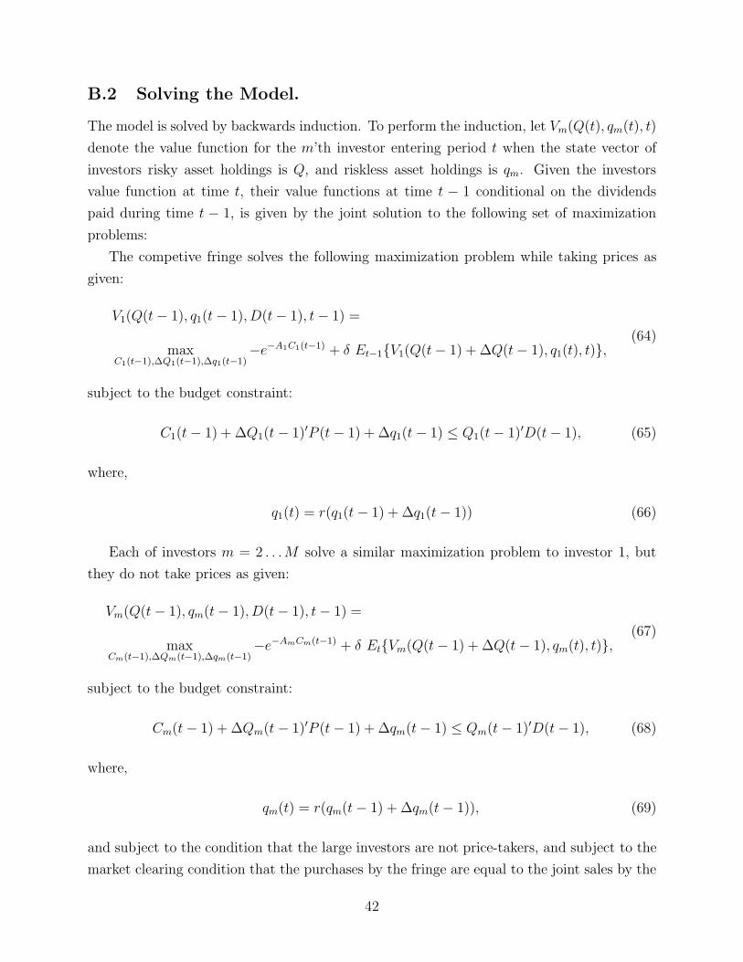
B.2 Solving the Model.

The model is solved by backwards induction. To perform the induction, let Vm(Q(t), qm(t), t)

denote the value function for the m’th investor entering period t when the state vector of

investors risky asset holdings is Q, and riskless asset holdings is qm. Given the investors

value function at time t, their value functions at time t − 1 conditional on the dividends

paid during time t − 1, is given by the joint solution to the following set of maximization

problems:

The competive fringe solves the following maximization problem while taking prices as

given:

V1(Q(t− 1), q1(t− 1), D(t− 1), t− 1) =

maxC1(t−1),∆Q1(t−1),∆q1(t−1)

−e−A1C1(t−1) + δ Et−1V1(Q(t− 1) + ∆Q(t− 1), q1(t), t),(64)

subject to the budget constraint:

C1(t− 1) + ∆Q1(t− 1)′P (t− 1) + ∆q1(t− 1) ≤ Q1(t− 1)′D(t− 1), (65)

where,

q1(t) = r(q1(t− 1) + ∆q1(t− 1)) (66)

Each of investors m = 2 . . .M solve a similar maximization problem to investor 1, but

they do not take prices as given:

Vm(Q(t− 1), qm(t− 1), D(t− 1), t− 1) =

maxCm(t−1),∆Qm(t−1),∆qm(t−1)

−e−AmCm(t−1) + δ EtVm(Q(t− 1) + ∆Q(t− 1), qm(t), t),(67)

subject to the budget constraint:

Cm(t− 1) + ∆Qm(t− 1)′P (t− 1) + ∆qm(t− 1) ≤ Qm(t− 1)′D(t− 1), (68)

where,

qm(t) = r(qm(t− 1) + ∆qm(t− 1)), (69)

and subject to the condition that the large investors are not price-takers, and subject to the

market clearing condition that the purchases by the fringe are equal to the joint sales by the

42

other large investors:

∆Q1 = −M∑

m=2

∆Qm. (70)

The solution to these equations in any time period is the Nash Equilibrium of a Stack-

elberg game in the trading of the risky and riskless assets, and in investors consumption

choices. The value functions above are defined conditional on D(t − 1), which is unknown

before time t− 1. To solve for the unconditional value of entering time t− 1 with risky and

riskless asset distributions Q(t−1), and q(t−1), it suffices to integrate the conditional value

functions with respect to the distribution of D(t− 1).

The value functions are solved for recursively by solving for the value function in period

T and working backwards. Fortunately, it is not too difficult to solve the model because

the value functions in each time period have a very simple form. In particular, in this

uncomplicated version of the model, each investors value function is an exponential linear

quadratic function of the state variables. To establish the form of the value functions, I

first show that if the value functions have a specific exponential linear-quadratic form in one

period of the model, they must have a similar form in earlier periods. I then show the value

functions have this form in the final period have this form, which completes the solution for

the structure of the value functions. Given these functions, the model can be recursively

solved for trades, and prices, and the properties of the model can be examined numerically.

B.3 The Form of the Value Functions.

The first step in solving the model is establishing that if the value functions have a sim-

ple structure in one period, then they have a similar structure in earlier periods. This is

established in the following proposition:

Proposition 6 For investors m = 1, . . .M , if Vm(Q, qm, t) has functional form:

Vm(Q, qm, t) = km(t)× exp(−Am(t)Q′vm(t) + .5Am(t)2Q′θm(t)Q− rAm(t)qm

)then the value functions at time t− 1 has form:

43

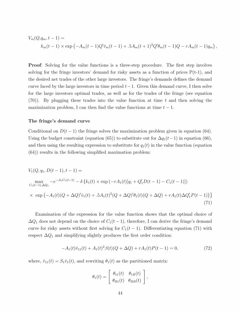
Vm(Q,qm, t− 1) =

km(t− 1)× exp(−Am(t− 1)Q′vm(t− 1) + .5Am(t+ 1)2Q′θm(t− 1)Q− rAm(t− 1)qm

),

Proof: Solving for the value functions is a three-step procedure. The first step involves

solving for the fringe investors’ demand for risky assets as a function of prices P(t-1), and

the desired net trades of the other large investors. The fringe’s demands defines the demand

curve faced by the large investors in time period t−1. Given this demand curve, I then solve

for the large investors optimal trades, as well as for the trades of the fringe (see equation

(70)). By plugging these trades into the value function at time t and then solving the

maximization problem, I can then find the value functions at time t− 1.

The fringe’s demand curve

Conditional on D(t− 1) the fringe solves the maximization problem given in equation (64).

Using the budget constraint (equation (65)) to substitute out for ∆q1(t−1) in equation (66),

and then using the resulting expression to substitute for q1(t) in the value function (equation

(64)) results in the following simplified maximation problem:

V1(Q, q1, D(t− 1), t− 1) =

maxC1(t−1),∆Q1

−e−A1C1(t−1) − δ k1(t)× exp (−rA1(t)[q1 +Q′1D(t− 1)− C1(t− 1)])

× exp(−A1(t)(Q+ ∆Q)′v1(t) + .5A1(t)

2(Q+ ∆Q)′θ1(t)(Q+ ∆Q) + rA1(t)∆Q′1P (t− 1)

)(71)

Examination of the expression for the value function shows that the optimal choice of

∆Q1 does not depend on the choice of C1(t− 1), therefore, I can derive the fringe’s demand

curve for risky assets without first solving for C1(t− 1). Differentiating equation (71) with

respect ∆Q1 and simplifying slightly produces the first order condition:

−A1(t)v11(t) + A1(t)2β(t)(Q+ ∆Q) + rA1(t)P (t− 1) = 0, (72)

where, v11(t) = S1v1(t), and rewriting θ1(t) as the partitioned matrix:

θ1(t) =

[θ11(t) θ1B(t)

θB1(t) θBB(t)

],

44

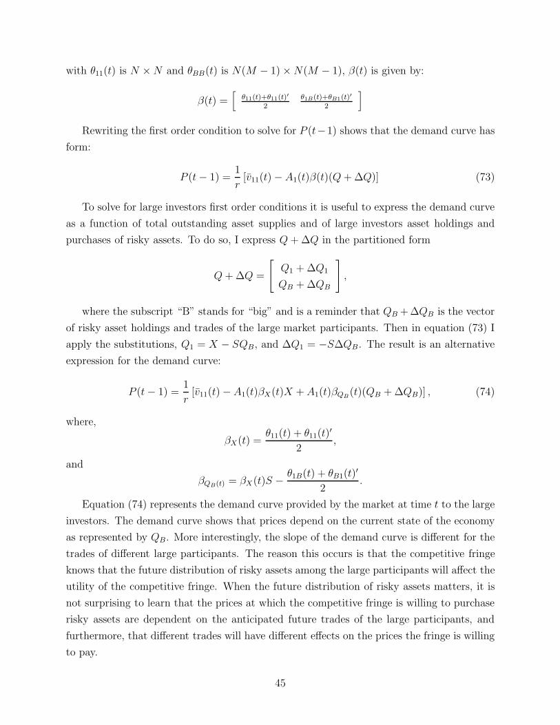
with θ11(t) is N ×N and θBB(t) is N(M − 1)×N(M − 1), β(t) is given by:

β(t) =[

θ11(t)+θ11(t)′2

θ1B(t)+θB1(t)′2

]

Rewriting the first order condition to solve for P (t−1) shows that the demand curve has

form:

P (t− 1) =1

r[v11(t)− A1(t)β(t)(Q+ ∆Q)] (73)

To solve for large investors first order conditions it is useful to express the demand curve

as a function of total outstanding asset supplies and of large investors asset holdings and

purchases of risky assets. To do so, I express Q+ ∆Q in the partitioned form

Q+ ∆Q =

[Q1 + ∆Q1

QB + ∆QB

],

where the subscript “B” stands for “big” and is a reminder that QB +∆QB is the vector

of risky asset holdings and trades of the large market participants. Then in equation (73) I

apply the substitutions, Q1 = X − SQB, and ∆Q1 = −S∆QB . The result is an alternative

expression for the demand curve:

P (t− 1) =1

r[v11(t)− A1(t)βX(t)X + A1(t)βQB

(t)(QB + ∆QB)] , (74)

where,

βX(t) =θ11(t) + θ11(t)

′

2,

and

βQB(t) = βX(t)S − θ1B(t) + θB1(t)′

2.

Equation (74) represents the demand curve provided by the market at time t to the large

investors. The demand curve shows that prices depend on the current state of the economy

as represented by QB. More interestingly, the slope of the demand curve is different for the

trades of different large participants. The reason this occurs is that the competitive fringe

knows that the future distribution of risky assets among the large participants will affect the

utility of the competitive fringe. When the future distribution of risky assets matters, it is

not surprising to learn that the prices at which the competitive fringe is willing to purchase

risky assets are dependent on the anticipated future trades of the large participants, and

furthermore, that different trades will have different effects on the prices the fringe is willing

to pay.

45

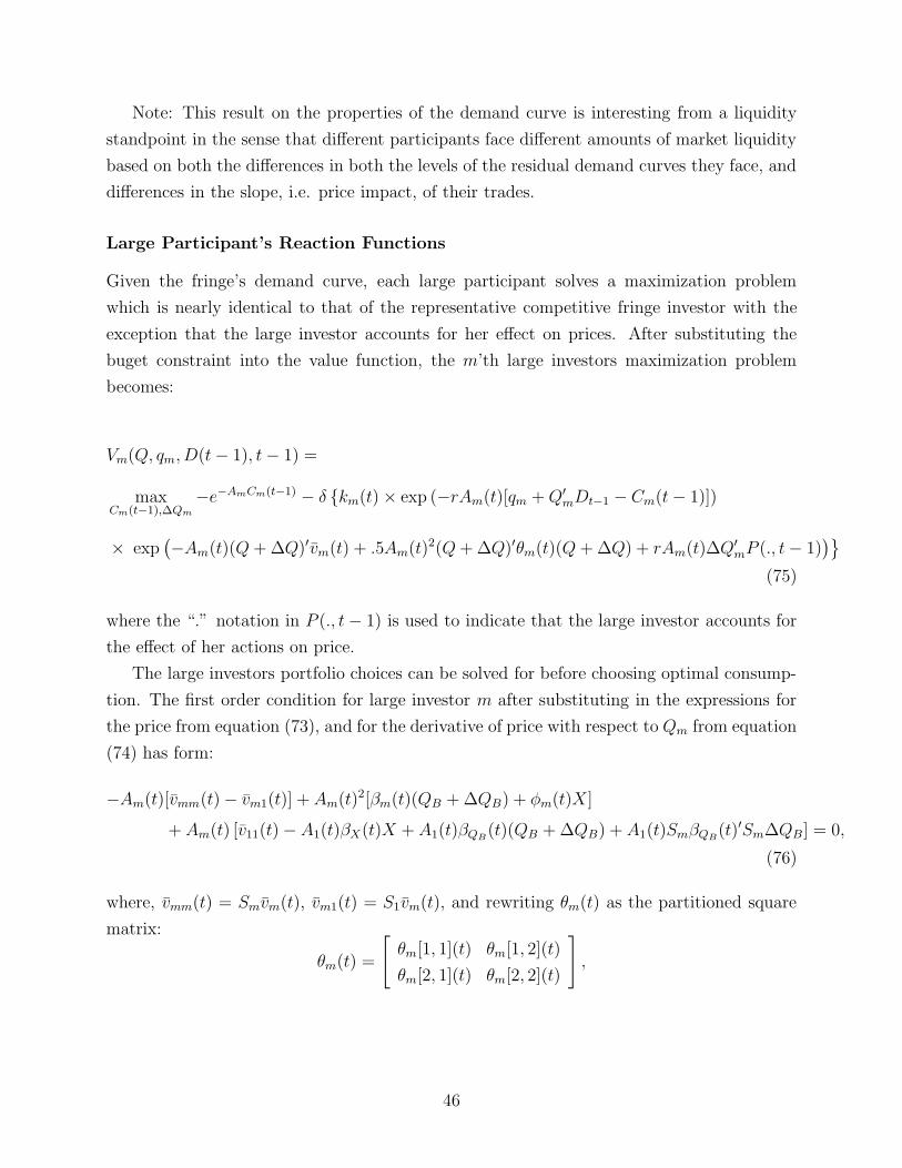
Note: This result on the properties of the demand curve is interesting from a liquidity

standpoint in the sense that different participants face different amounts of market liquidity

based on both the differences in both the levels of the residual demand curves they face, and

differences in the slope, i.e. price impact, of their trades.

Large Participant’s Reaction Functions

Given the fringe’s demand curve, each large participant solves a maximization problem

which is nearly identical to that of the representative competitive fringe investor with the

exception that the large investor accounts for her effect on prices. After substituting the

buget constraint into the value function, the m’th large investors maximization problem

becomes:

Vm(Q, qm, D(t− 1), t− 1) =

maxCm(t−1),∆Qm

−e−AmCm(t−1) − δ km(t)× exp (−rAm(t)[qm +Q′mDt−1 − Cm(t− 1)])

× exp(−Am(t)(Q+ ∆Q)′vm(t) + .5Am(t)2(Q+ ∆Q)′θm(t)(Q+ ∆Q) + rAm(t)∆Q′

mP (., t− 1))

(75)

where the “.” notation in P (., t− 1) is used to indicate that the large investor accounts for

the effect of her actions on price.

The large investors portfolio choices can be solved for before choosing optimal consump-

tion. The first order condition for large investor m after substituting in the expressions for

the price from equation (73), and for the derivative of price with respect to Qm from equation

(74) has form:

−Am(t)[vmm(t)− vm1(t)] + Am(t)2[βm(t)(QB + ∆QB) + φm(t)X]

+ Am(t) [v11(t)− A1(t)βX(t)X + A1(t)βQB(t)(QB + ∆QB) + A1(t)SmβQB

(t)′Sm∆QB] = 0,

(76)

where, vmm(t) = Smvm(t), vm1(t) = S1vm(t), and rewriting θm(t) as the partitioned square

matrix:

θm(t) =

[θm[1, 1](t) θm[1, 2](t)

θm[2, 1](t) θm[2, 2](t)

],

46

where θm[1, 1](t) is N ×N and θm[2, 2](t) is N(M − 1)×N(M − 1), βm(t) is given by:

βm(t) =(θm[1, 1](t) + θm[1, 1](t)′)S

2− (Smθm[1, 2](t)′ + Smθm[2, 1](t)′)S

2

− θm[1, 2](t) + θm[2, 1](t)′

2+Smθm[2, 2](t) + Smθm[2, 2](t)′

2,

(77)

and φm(t) is given by:

φm(t) =(Smθm[1, 2](t)′ + Smθm[2, 1](t)′)

2− (θm[1, 1](t) + θm[1, 1](t)′)

2. (78)

Rearrangement of the first order condition for the m′th large investor produces a reaction

function with form:

πm(t)∆QB = [vmm(t)− v11(t)− vm1(t)] + ρm(t)X + ξm(t)QB, (79)

where,

πm(t) = Am(t)βm(t) + A1(t)βQB(t) + A1(t)SmβQB

(t)′Sm (80)

ξm(t) = −Am(t)βm(t)− A1(t)βQB(t) (81)

ρm(t) = A1(t)βX(t)− Am(t)φm(t) (82)

Stacking the (M-1) reaction functions produces a system of (M − 1)N linear equations

in (M − 1)N unknowns:

Π(t)∆QB = χ(v(t)) + ρ(t)X + ξ(t)QB (83)

where Π(t) = stackMm=2(πm(t)) and χ(vt) = stackM

m=2(vmm(t) − v11(t) − vm1(t)), and ξ(t) =

stackMm=2(ξm(t)).

Assume that Π(t) is invertible. Then the solution for ∆QB is unique, and the solution

for ∆Q1 is −S∆QB . After making the substitution Q1 + SQB = X, the solution for ∆Q =

(∆Q′1,∆Q

′B)′ can be written as:

∆Q = H0(t) +H1(t)Q. (84)

47

where,

H0(t) =

(−SΠ(t)−1χ(v(t))

Π(t)−1χ(v(t))

), and H1(t) =

(−SΠ(t)−1ρ(t) −SΠ(t)−1(ξ(t) + ρ(t)S)

Π(t)−1ρ(t) Π(t)−1(ξ(t) + ρ(t)S)

).

(85)

Given the solution for ∆Q, it is convenient to write Q+ ∆Q as

Q+ ∆Q = G0(t) +G1(t)Q (86)

where G0(t) = H0(t) and G1(t) = H1(t) + I.

Finally, with this notation, we have

∆Qm = Sm[H0(t) +H1(t)Q] (87)

Plugging these expressions back into the value function for the m’th investor (it could

be the competitive investor or a large investor) and simplifying (details to follow shortly),

shows that the value function conditional on D(t− 1) has form:

Vm(Q, qm, D(t− 1), t− 1) = maxCm(t−1)

−e−AmCm(t−1) − δe[rA1(t)Cm(t−1)] × ψm(t− 1) (88)

where,

ψm(t−1) = km(t−1)×e−rAm(t)[qm(t−1)+Qm(t−1)′D(t−1)]×e[−Am(t)Q(t−1)′ vm(t−1)+.5Am(t)2Q(t−1)′ θm(t−1)Q(t−1)]

Solving the above expression for optimal Cm(t− 1) and plugging the solution back into

the value function shows that:

Vm(Q, qm, D(t− 1), t− 1) = − [1 + (1/r∗(t))]× [r∗(t)δ]1

1+r∗(t) × [ψm(t− 1)]1

1+r∗(t) , (89)

where,

r∗(t) = rAm(t)/Am (90)

Finally, taking expectations of the right hand side of equation (89) with respect to the

48

distribution of dividends provides the final form of the value function at time t− 1,

Vm(Q,qm, t− 1) =

km(t− 1)×− exp[−Am(t− 1)Q′vm(t− 1) + .5Am(t− 1)2Q′θm(t− 1)Q− r Am(t− 1)qm

](91)

Additional Details on Derivation of Vm(Q, qm, t− 1)

Many details were left out of the derivation of the value function for large investors. To

fill in the details, if one plugs the expression for Q + ∆Q (equation (86)) into the demand

curve (equation (73)) to solve for P (t− 1), and then one plugs the solutions for P , Q+ ∆Q,

and ∆Q (equation (84)), into the conditional value function (equation (75)) and simplifies,

one finds that the time varying parameters in ψm(t− 1) are related to known parameters as

follows:

km(t− 1) = km(t)×exp(−Am(t)G0(t)

′vm(t) + .5Am(t)2G0(t)′θm(t)G0(t) + Am(t)H0(t)

′S ′m[v11(t)− A1(t)β1(t)G0(t)])

(92)

vm(t− 1) =G1(t)′vm(t)− Am(t)G1(t)

′(θm(t) + θm(t)′

2

)G0(t)

−H1(t)′S ′m [v11(t)− A1(t)β1(t)G0(t)] + A1(t)G1(t)

′β(t)′SmH0(t)

(93)

θm(t− 1) = G1(t)′θm(t)G1(t)− [2A1(t))/Am(t)]H1(t)

′Smβ(t)G1(t) (94)

The rest of the solution of the value function is straightforward. Let,

Am(t− 1) =Am(t)

1 + r∗(t). (95)

Using expression for Am(t − 1) to substitute out for Am(t) in equation (89) and then

taking expectations with respect to both sides and simplifiying the results shows that:

vm(t− 1) = vm(t− 1) + rS ′mD (96)

θm(t− 1) = (1 + r∗(t))θm(t− 1) + r2S ′mΩSm (97)

km(t− 1) = (km(t− 1))1/(1+r∗(t)) [1 + (1/r∗(t))]× [r∗(t)δ]1/(1+r∗(t)) (98)

49

These final details on the derivation of the value function at time t−1 complete the proof

of Proposition 6. 2.

To prove that the value function in all time periods has the same form as that in propo-

sition 6, it suffices to establish that the value function in period T − 1, the last period where

trade or consumption decisions are made, has this form. Recall that in period T , no trade

takes place, instead, asset payoffs are consumed. Therefore, an investor who enters period

T with Qm(T ) risky assets and qm(t) receives interest and dividends on the their holdings,

and then consume it. Thus, their utility at time T conditional on asset payoffs D(T ) is

− exp [−AmQm(T )′D(T ) + qm(T )]

and hence the ex-ante expected utility of carrying these assets into period T is

− exp[−AmQm(T )′D + .5A2

mQm(T )′ΩQm(T ) + qm(T )]

Hence, the value of entering time period T−1 with risky asset distribution Q, and riskless

asset holdings qm can be found from solving maximization problems which are analogous to

those given by equations (64), and (67). In particular, the set of investor value functions at

time t − 1 are defined as the joint solution when each investor m solves the maximization

problem

Vm(Q, qm, T − 1) =

maxCm(T−1),∆Qm,∆qm

−e−AmCm(t−1) − δe(−Am(Qm+∆Qm)′D+.5A2m(Qm+∆Qm)′Ω(Qm+∆Qm)+qm(T ))

(99)

where,

qm(T ) = r(qm + ∆qm),

subject to the budget constraint,

Cm(t− 1) + ∆Q′mP (T − 1) + ∆qm ≤ Q′

mD(T − 1),

and subject to the market clearing requirement:

∆Q1 = −M∑

m=2

∆Qm.

50

Recall that investor 1 takes prices as given, while investors 2 through M account for the

effect that their trades have on prices.

As in the earlier maximization problem, assuming the constraints are binding, I can use

the budget constraint to substitute out for ∆qm(T − 1) in the expression for qm(T ) and

then substitute the result into the expression being maximized. The result is the following

optimization problem for each investor m:

Vm(Q, qm, D(T − 1), T − 1) =

maxCm(T−1),∆Qm

−e−AmCm(T−1) − δ exp (−rAm(T )[qm +Q′mD(T − 1)− Cm(T − 1)])

× exp(−Am(Qm + ∆Qm)′D + .5A2

m(Qm + ∆Qm)′Ω(Qm + ∆Qm) + rAm∆Q′mP (., T − 1)

)(100)

With substitutions, this maximization can be rewritten in the form:

Vm(Q, qm, D(T − 1), T − 1) =

maxCm(T−1),∆Qm

−e−AmCm(T−1) − δ km(T )× exp (−rAm(T )[qm +Q′mDT−1 − Cm(T − 1)])

× exp(−Am(T )(Q+ ∆Q)′vm(T ) + .5Am(T )2(Q+ ∆Q)′θm(T )(Q+ ∆Q) + rAm(T )∆Q′

mP (., T − 1))

(101)

where,

km(T ) = 1, (102)

vm(T ) = S ′mD (103)

θm(T ) = S ′mΩSm (104)

Am(T ) = Am (105)

Since the investors transformed maximization problem is exactly analogous to equation

equation (75), an intermediate step in proving proposition 6, it follows that the value function

at time T −1 has the same form as given in proposition 6. This completes the induction and

and establishes that the value function in all time periods has the same form as that given

in proposition 6. 2

51

Fringe’s Last Period Demand Curve

Manipulation of the fringe’s first order condition for its choices of risky assets in period T −1

shows that the fringe’s demand curve during time period T − 1 has the form:

P (T − 1) =1

r

(D − A1Ω(Q1 + ∆Q1)

)(106)

=1

r

(D − A1ΩQ1 + A1Ω

M∑m=2

∆Q1

), (107)

where the last line of the expression for demand uses the substition that the risky asset

purchases of the fringe are equal to the net sales of the large investors.

An important feature of this demand curve is that the slope of the demand curve is the

same for the orderflow of each large investor. The reason the model has this feature in the

final time period is because the fringe’s trades with each large investor alter the fringe’s

consumption in time period T , but it does not alter the strategic environment in period

T because there is no trading in the last period. In earlier periods of the model, different

distributions of risky assets among the large investors alter the strategic environment and

hence the fringe’s future consumption. As a result, the trades of different large investors

have different price impacts (for the same trade size).

Second Order Conditions

An implicit assumption in the analysis to this point is that the first order conditions which

describe investor’s reaction functions, and the fringe’s demand curve actually provide each

investor’s best response to the actions of the other participants.21 To establish that investors

portfolio choices are best responses, it suffices to show that investors value functions are

concave in their holdings of risky assets. To establish concavity in changes in risky asset

holdings for the large investors (investors 2, . . .M), inspection of equation 75 shows that it

suffices to differentiate the following expression twice with respect to ∆Qm and then examine

whether the result is negative definite for every period t.

exp(−Am(t)(Q+ ∆Q)′vm(t) + .5Am(t)2(Q+ ∆Q)′θm(t)(Q+ ∆Q) + rAm(t)∆Q′

mP (., t− 1))

21The obvious case where things might break down is if the solutions to the first order conditions areactually local minima instead of global maxima.

52

Differentiation shows that a sufficient condition for negative definiteness is that for each

large partipant in each time period, the matrix

Am(t)2(−s1 + sm)

(θm(t) + θm(t)′

2

)(−s1 + sm)′ + rAm(t)[P∆Qm(.) + P∆Qm(.)′] >> 0

, where >> denotes positive definiteness.

A similar condition holds for the competitive fringe. Specifically, the second order con-

dition for the fringe’s holdings of risky assets requires that the matrix

A1(t)2(s1)

(θ1(t) + θ1(t)

′

2

)(s1)

′ >> 0

.

I have not yet formally established under what circumstances the second order conditions

are satisfied. However, these conditions are satisfied in all my analysis of the multiperiod

model which I have performed so far.

B.4 The Multi-Period Model with Liquidity Shocks.

Here I consider how liquidity shocks affect the equilibrium reaction functions and value

functions. In particular, I look first at the effect of a one-time surprise liquidity shock

occuring to a single participant. It is assumed that in all future periods beyond that where

the shock occured there will not be any further shocks. This assumption guarantees that

the value function for periods beyond where the shock occured are valid.

I assume that liquidity shocks occur in a period before trading occurs but after dividends

are known. Any large investor that experiences a liquidity shock of size L at time t−1 solves

the maximization problem:

maxCm(t−1),∆Qm(t−1),∆qm(t−1)

−e−AmCm(t−1) − δkm(t)e−Am(t)(Q+∆Q)′vm(t)+.5Am(t)2(Q+∆Q)′θm(t)(Q+∆Q)−Am(t)r(qm+∆qm)

(108)

such that

qm + ∆qm ≥ 0 (109)

∆qm + C(t− 1) + ∆Q′mP ≤ Q′

mDt−1 − L (110)

The first constraint is a borrowing constraint. When this constraint is binding, then risky

assets need to be sold to meet the liquidity shock (−L). The second constraint is always

binding because the marginal utility of consumption is strictly increasing.

53

The interesting case to consider is the one in which both constraints are binding. When

both are binding, one can substitute for qm +∆qm and for Ct−1. This reduces the maximiza-

tion problem to the following expression:

max∆Qm

−e−Am(Q′mDt−1−L+qm−∆Q′

mP ) − δkm(t)e−Am(t)(Q+∆Q)′vm(t)+.5Am(t)2(Q+∆Q)′θm(t)(Q+∆Q)

(111)

The first order condition for this maximization problem is the reaction function for the

investor who receives a liquidity shock. After simplication, the reaction function has form:

αm(t)∆QB = (−ηm(t)Am(t)/r)v11(t) + Am(t)(vmm(t)− vm1(t)) + λm(t)X + γm(t)QB

(112)

where,

αm(t) = ηm(t)(Am/r)[A1(t)βQB(t) + A1(t)Smβ

′QB(t)Sm

]+ Am(t)2βm(t) (113)

ηm(t) =e−Am(Q′

mDt−1−L+qm−∆Q′mP )

δkm(t)e−Am(t)(Q+∆Q)′vm(t)+.5Am(t)2(Q+∆Q)′θm(t)(Q+∆Q)(114)

λm(t) = ηm(t)(Am/r)A1(t)βX(t)− Am(t)2φm(t) (115)

γm(t) = ηm(t)(Am/r)A1(t)Smβ′QB(t)Sm − αm(t) (116)

Because ηm(t) is a nonlinear function of all participants trades, the reaction function for

the large participant hit with a liquidity shock is highly nonlinear. Nevertheless, solving for

equilibrium trades is still fairly straightforward. To solve the model, I guess a value for ηm(t).

For given ηm(t), the above reaction function is linear. Since all other reaction functions are

linear as well, I can solve for ∆QB given ηm(t), and then given ∆QB, I can solve for ηm(t).

When I find a fixed point for ηm(t), then I have solved for the equilibrium trades and can

hence compute the value function for entering the period with risky asset distribution Q

when the m′th large participant is hit with a liquidity shock of size L.

B.5 Multiperiod Model with Competitive Market Participants

It is useful to contrast the behavior in the multi-market model with large investors with the

behavior of asset prices and trades in the same model when all investors are price takers.

The derivation of prices and trades in this case is a special case of the derivation with large

54

investors. It is also a special case of the derivation in Stapleton and Subramanyam (1978).

Therefore, I will not provide a detailed derivation, but will instead just provide results.

In time period T − 1, the last period of trade, equilibrium asset prices are given by

P (T − 1) =1

r

(D − 1∑M

i=1(1/Am)ΩX

)(117)

The CAPM is clearly satisfied in the last period of trade. In all earlier periods, prices

satisfy the difference equation:

P (t− 1)1

r

(P (t) + D − 1∑M

i=1(1/Am(t))ΩX

)(118)

where,

Am(t− 1) =Am(t)r

1 + r∗(t), (119)

and

r∗(t) = rAm(t)/Am (120)

It follows that in each period prior to the last period, one-period excess returns (P (t) +

D(t)− rP (t− 1)) satisfy the CAPM with market prices of risk that vary through time.

Moreover, in the perfectly competitive model, trade only occurs in period 1, and not

thereafter.

55

BIBLIOGRAPHY

Almgren, R., and N. Chriss, “Optimal Execution of Portfolio Transactions,” 2000, Journalof Risk, 3, Winter 2000/2001, 5-39.

Basak, S., “Consumption choice and asset pricing with a non-price taking agent,” 1997,Economic Theory, 10, 437-462.

Basak, S., and A. Pavlova, 2001, “Monopoly Power and the Firm’s Valuation: A DynamicAnalysis of Short versus Long-Term Policies,” Working Paper, London Business School.

Boudoukh, J., and R.F. Whitelaw, 1993, “Liquidity as a Choice Variable: A Lesson fromthe Japanese Government Bond Market,” Review of Financial Studies, 6, 265-292.

Cao, H.H., and R.K. Lyons, 1999, “Inventory Information,” mimeo, Haas School of Busi-ness, University of California at Berkeley.

Chan, L.K.C., and J. Lakonishok, 1995, “The Behavior of Stock Prices Around InstitutionalTrades,” Journal of Finance, 50, 1147-1174.

Cherubini, U., and G. Della Lunga, 2001, “Liquidity and Credit Risk,” Mathematical Fi-nance, Forthcoming.

Constantinides, G.M., 1986, “Capital Market Equilibrium with Transaction Costs,”, Jour-nal of Political Economy, 94, 842-862.

Corsetti, G., Pesenti, P., and N. Roubini, 2001, “The role of large players in currencycrises,” Mimeo.

DeMarzo, P.M., and B. Urosevic, 2000 “Optimal Trading by a Large Shareholder,” WorkingPaper, Haas School of Business, University of California at Berkeley.

Demarzo, P.M., and D. Duffie, 199, “A Liquidity-Based Model of Security Design,” Econo-metrica, 67, 65-99.

Duffie, D., Garleanu, N., and L.H. Pedersen, 2001, “Valuation in Dynamic BargainingMarkets,” Working Paper, Graduate School of Business, Stanford University.

Eisfeldt, A., 2001, “Endogenous Liquidity in Asset Markets,” Mimeo, Kellog GraduateSchool of Management, Northwestern University, April.

Glosten, L.R., and P.R. Milgrom, 1985, “Bid, Ask, and Transaction Prices in a SpecialistMarket with Heterogeneously Informed Traders,” Journal of Financial Economics, 14,71-100

Grinblatt, M.S., and S.A. Ross, 1985, “Market Power in a Securities Market with Endoge-nous Information,” Quarterly Journal of Economics 100, 1143-1167.

Heaton, J., and D.J. Lucas, 1996, “Evaluating the Effects of Incomplete Markets on RiskSharing and Asset Pricing,” Journal of Political Economy, 104, 443-487.

Holmstrom, B., and J. Tirole, 1998, “LAPM: A Liquidity-Based Asset Pricing Model,”NBER Working Paper 6673.

Huang, M., “Liquidity Shocks and Equilibrium Liquidity Premia,” Mimeo, Graduate Schoolof Business, Stanford University.

56

Jarrow, R.A., 1992, “Market Manipulation, Bubbles, Corners, and Short Squeezes,” Journalof Financial and Quantitative Analysis 27, no. 3, 311-336.

Kihlstrom, R., 2001, “Monopoly Power in Dynamic Securities Markets,” Working Paper,The Wharton School, University of Pennsylvania.

Krishnamurthy, A., 2001, “The Bond, Old-Bond Spread,” Mimeo, Northwestern University,June.

Kyle, A.S., and Xiong, W., 2001, “Contagion as a Wealth Effect,” Journal of Finance, 56,1401-1440.

Kyle, A.S, 1989, “Informed Speculation with Imperfect Competition,” Review of EconomicStudies, 56, 317-356.

Kyle, A.S., 1985, “Continuous Auctions and Insider Trading,” Econometrica, 53, 1315-1335.

Lindenberg, E.B., 1979, “Capital Market Equilibrium with Price Affecting InsitutionalInvestors,” in Portfolio Theory 25 Years After: Essays in Honor of Harry Markowitz,Elton, E.J., and M.J. Gruber, eds., North Holland, pp. 109-124.

Routledge, B.R., and S.E. Zin, 2001, “Model Uncertainty and Liquidity,” Mimeo, July.

Stapleton, R.C., and M.G. Subrahmanyam, 1978, “A Multiperiod Equilibrium Asset PricingModel,” Econometrica, 46, 1077-1096.

Subramanian, A., December 2000, “Optimal Liquidation for a Large Investor,” Mimeo.

Subramanian, A., and R.A. Jarrow, 1997, “The Liquidity Discount,” Mimeo, JohnsonSchool of Management, Cornell University.

Vayanos, D., 2001, “Strategic Trading in a Dynamic Noisy Market,” Journal of Finance,Forthcoming.

Vayanos, D., 1999, “Strategic Trading and Welfare in a Dynamic Market,” Review of Eco-nomic Studies, 66, 219-254.

Vayanos, D., and J.L. Vila, 1999, “Equilibrium interest rate and liquidity premium withtransaction costs,” Economic Theory, 13, 509-539.

Vayanos, D., 1998, “Transaction Costs and Asset Prices: A Dynamic Equilibrium Model,”Review of Financial Studies, 11, 1-58.

57

Table 1: Multiperiod Model When Investors Have Same Risk Aversion

A. Initial Conditions: Time 0.Investor #

1 2 3 4 5 6

Price-Taker Yes No No No No No

Risk Aversion 1.0 1.0 1.0 1.0 1.0 1.0

Risky Asset Endowment 2.0 2.0 2.0 2.0 2.0 2.0

B. Dynamics: Price and Investor 1’s Demand Curve ParametersEquilibrium Demand Curve Demand Curve Slopes by Investor #

Time Price Intercept 2 3 4 5 6

1 20.3562 12.9515 0.7405 0.7405 0.7405 0.7405 0.7405

2 15.7578 8.1572 0.7601 0.7601 0.7601 0.7601 0.7601

3 11.2602 3.2201 0.8040 0.8040 0.8040 0.8040 0.8040

4 6.9313 -1.9198 0.8851 0.8851 0.8851 0.8851 0.8851

5 2.9412 -6.8627 0.9804 0.9804 0.9804 0.9804 0.9804

C. Dynamics: End of Period Risky Asset HoldingsInvestor #

Time 1 2 3 4 5 6

1 2.0000 2.0000 2.0000 2.0000 2.0000 2.0000

2 2.0000 2.0000 2.0000 2.0000 2.0000 2.0000

3 2.0000 2.0000 2.0000 2.0000 2.0000 2.0000

4 2.0000 2.0000 2.0000 2.0000 2.0000 2.0000

5 2.0000 2.0000 2.0000 2.0000 2.0000 2.0000

Notes: For the multi-period model, given the initial conditions in panel A, the table presentsthe evolution of risky asset prices (panel B), investors end of period risky asset holdings(panel C), and the liquidity available to large investors as measured by the slope of theprice function with response to their order flow (panel B, last 5 columns). Because investorsinitial asset allocations are pareto optimal, investors do not trade away from their initialasset holdings. Further details are provided in section 4.6 of the text.

58

Table 2: Multiperiod Model: Baseline 1

A. Initial Conditions: Time 0.Investor #

1 2 3 4 5 6

Price-Taker Yes No No No No No

Risk Aversion 1.0 1.0 2.0 3.0 4.0 5.0

Risky Asset Endowments 3.6548 3.6548 1.8274 1.2183 0.9137 0.7310

B. Liquidity Indicators: Price and Price Function ParametersEquilibrium Price Function Price Function Slope to Purchases by Investor #

Time Price Intercept 2 3 4 5 6

1 16.5950 7.4169 1.1518 1.0836 1.0552 1.0396 1.0297

2 12.3288 3.4983 1.1070 1.0438 1.0162 1.0009 0.9911

3 8.2470 -0.2579 1.0626 1.0074 0.9819 0.9674 0.9580

4 4.4733 -3.8013 1.0235 0.9841 0.9643 0.9525 0.9446

5 1.3188 -6.8627 0.9804 0.9804 0.9804 0.9804 0.9804

C. End of Period Risky Asset HoldingsInvestor #

Time 1 2 3 4 5 6

1 3.6548 3.6548 1.8274 1.2183 0.9137 0.7310

2 3.6548 3.6548 1.8274 1.2183 0.9137 0.7310

3 3.6548 3.6548 1.8274 1.2183 0.9137 0.7310

4 3.6548 3.6548 1.8274 1.2183 0.9137 0.7310

5 3.6548 3.6548 1.8274 1.2183 0.9137 0.7310

Notes: The table provides the the initial conditions used for the first baseline multiperiodmodel (panel A), and then presents the baseline evolution of risky asset prices (panel B),and investors end of period risky asset holdings (panel C), as well as the liquidity availableto large investors as measured by the slope of the price function with response to theirorder flow (panel B, last 5 columns). Because investors initial asset allocations are paretooptimal, investors do not trade away from their initial baseline allocations. Further detailsare provided in section 4.6 of the text.

59

Table 3: Endowment Shock to Price-Taking Investor: Baseline 1

A. Initial Conditions: Time 0.Investor #

1 2 3 4 5 6

Price-Taker Yes No No No No No

Risk Aversion 1.0 1.0 2.0 3.0 4.0 5.0

Endowment Shock Yes No No No No No

Risky Asset Endowments 4.6548 3.6548 1.8274 1.2183 0.9137 0.7310

Change from Baseline 1.0 0.0 0.0 0.0 0.0 0.0

B. Dynamics: Price and End of Period Risky Asset HoldingsRisky Asset Holdings by Investor #

Time Price Intercept 1 2 3 4 5 61 15.7412 5.9599 4.0964 3.8026 1.9515 1.3253 1.0083 0.8159

2 11.6492 2.1313 3.9975 3.8615 1.9792 1.3373 1.0112 0.8133

3 7.6706 -1.5212 3.9763 3.8984 1.9858 1.3332 1.0029 0.8034

4 4.0099 -4.9433 3.9686 3.9253 1.9858 1.3274 0.9961 0.7968

5 1.0158 -7.8431 3.9639 3.9446 1.9832 1.3228 0.9920 0.7935

C. Price and Quantity Dynamics: Differences from Baseline 1 (Table 2)Risky Asset Holdings by Investor #

Time Price Intercept 1 2 3 4 5 61 -0.8537 -1.4571 0.4416 0.1478 0.1241 0.1070 0.0946 0.0849

2 -0.6796 -1.3670 0.3427 0.2067 0.1517 0.1190 0.0975 0.0823

3 -0.5764 -1.2633 0.3214 0.2436 0.1584 0.1149 0.0892 0.0724

4 -0.4634 -1.1419 0.3138 0.2704 0.1584 0.1092 0.0824 0.0658

5 -0.3030 -0.9804 0.3091 0.2898 0.1558 0.1046 0.0783 0.0625

Notes: For the multi-period model, given the deviation from baseline initial conditions whichis detailed in panel A, the table presents the resulting evolution of risky asset prices andrisky asset holdings (panel B), and contrasts the new prices and holdings against the baseline(panel C). Further details are presented in section 4.6.

60

Table 4: Effects of Endowment Shock to Investor 2

A. Initial Conditions: Time 0.Investor #

1 2 3 4 5 6

Price-Taker Yes No No No No No

Risk Aversion 1.0 1.0 2.0 3.0 4.0 5.0

Endowment Shock No Yes No No No No

Risky Asset Endowments 3.6548 4.6548 1.8274 1.2183 0.9137 0.7310

Change from Baseline 0.0 1.0 0.0 0.0 0.0 0.0

B. Dynamics: Price and End of Period Risky Asset HoldingsRisky Asset Holdings by Investor #

Time Price Intercept 1 2 3 4 5 61 16.0644 5.9599 3.8498 4.4508 1.8332 1.2208 0.9146 0.7309

2 11.7915 2.1313 3.8963 4.3005 1.8664 1.2478 0.9377 0.7513

3 7.7513 -1.5212 3.9167 4.1807 1.9018 1.2740 0.9584 0.7684

4 4.0548 -4.9433 3.9315 4.0862 1.9335 1.2950 0.9737 0.7801

5 1.0349 -7.8431 3.9444 4.0153 1.9593 1.3099 0.9836 0.7874

C. Price and Quantity Dynamics: Differences from Baseline (Table 2)Risky Asset Holdings by Investor #

Time Price Intercept 1 2 3 4 5 61 -0.5306 -1.4571 0.1950 0.7959 0.0058 0.0025 0.0009 -0.0001

2 -0.5373 -1.3670 0.2415 0.6456 0.0390 0.0296 0.0240 0.0203

3 -0.4957 -1.2633 0.2618 0.5259 0.0743 0.0558 0.0447 0.0374

4 -0.4185 -1.1419 0.2767 0.4314 0.1061 0.0767 0.0599 0.0492

5 -0.2839 -0.9804 0.2896 0.3605 0.1319 0.0916 0.0699 0.0565

Notes: For the multi-period model, given the deviation from baseline initial conditions whichis detailed in panel A, the table presents the resulting evolution of risky asset prices andrisky asset holdings (panel B), and contrasts the new prices and holdings against the baseline(panel C). Further details are presented in section 4.6.

61

Table 5: Effects of Endowment Shock to Investor 6

A. Initial Conditions: Time 0.Investor #

1 2 3 4 5 6

Price-Taker Yes No No No No No

Risk Aversion 1.0 1.0 2.0 3.0 4.0 5.0

Endowment Shock No No No No No Yes

Risky Asset Endowments 3.6548 3.6548 1.8274 1.2183 0.9137 1.7310

Change from Baseline 0.0 0.0 0.0 0.0 0.0 1.0

B. Dynamics: Price and End of Period Risky Asset HoldingsRisky Asset Holdings by Investor #

Time Price Intercept 1 2 3 4 5 61 15.8483 5.9599 3.9762 3.7181 1.8759 1.2573 0.9465 1.2259

2 11.6315 2.1313 4.0043 3.7982 1.9323 1.3009 0.9820 0.9823

3 7.6507 -1.5212 3.9915 3.8609 1.9654 1.3211 0.9954 0.8658

4 3.9996 -4.9433 3.9777 3.9059 1.9795 1.3255 0.9960 0.8154

5 1.0121 -7.8431 3.9676 3.9368 1.9824 1.3233 0.9927 0.7972

C. Price and Quantity Dynamics: Differences from Baseline (Table 2)Risky Asset Holdings by Investor #

Time Price Intercept 1 2 3 4 5 61 -0.7467 -1.4571 0.3214 0.0633 0.0485 0.0390 0.0328 0.4950

2 -0.6973 -1.3670 0.3495 0.1434 0.1049 0.0826 0.0683 0.2513

3 -0.5963 -1.2633 0.3367 0.2061 0.1380 0.1028 0.0817 0.1348

4 -0.4737 -1.1419 0.3229 0.2511 0.1521 0.1073 0.0823 0.0844

5 -0.3067 -0.9804 0.3128 0.2820 0.1550 0.1050 0.0790 0.0662Notes: For the multi-period model, given the deviation from baseline initial conditions whichis detailed in panel A, the table presents the resulting evolution of risky asset prices andrisky asset holdings (panel B), and contrasts the new prices and holdings against the baseline(panel C). Further details are presented in section 4.6.

62

Figure 1: Baseline Risky Asset Holdings

Notes: Blah blah blah.

63

Figure 2: Baseline Prices

64

Figure 3: Deviations from Baseline Asset Holdings due to Cash Flow Shock toLarge Investor 2

65

Figure 4: Deviations from Baseline Asset Holdings due to Cash Flow Shock toLarge Investor 6

66

Figure 5: Deviations from Baseline Prices due to Cash Flow Shocks to LargeInvestors 2, 3, 4, 5, and 6

67