Large Eddy Simulations on a pitching airfoil: Analysis of ...

HAL Id: hal-01630084https://hal.archives-ouvertes.fr/hal-01630084

Submitted on 11 Jan 2018

HAL is a multi-disciplinary open accessarchive for the deposit and dissemination of sci-entific research documents, whether they are pub-lished or not. The documents may come fromteaching and research institutions in France orabroad, or from public or private research centers.

L’archive ouverte pluridisciplinaire HAL, estdestinée au dépôt et à la diffusion de documentsscientifiques de niveau recherche, publiés ou non,émanant des établissements d’enseignement et derecherche français ou étrangers, des laboratoirespublics ou privés.

Large Eddy Simulations on a pitching airfoil: Analysis ofthe reduced frequency influence

Nathanaël Guillaud, Guillaume Balarac, Eric Goncalves da Silva

To cite this version:Nathanaël Guillaud, Guillaume Balarac, Eric Goncalves da Silva. Large Eddy Simulations on apitching airfoil: Analysis of the reduced frequency influence. Computers and Fluids, Elsevier, 2018,161, pp.1-13. �10.1016/j.compfluid.2017.11.002�. �hal-01630084�

https://hal.archives-ouvertes.fr/hal-01630084

https://hal.archives-ouvertes.fr

Large Eddy Simulations on a pitching airfoil: Analysis of the reduced

frequency influence

N Guillaud1, G Balarac2 and E Goncalves3

1 HydroQuest SAS, INOVALLIA, batiment B, 16 chemin de Malacher, 38240 Meylan, France

2 Univ. Grenoble Alpes / CNRS, LEGI UMR 5519, Grenoble, F-38041, France

3 ISAE-ENSMA/CNRS, Pprime UPR 3346, Teleport 2, 1 Avenue

Clement Ader, BP 40109, 86961 Futuroscope Chasseneuil Cedex, France

(Dated: June 7, 2017)

Abstract

Large Eddy Simulations (LES) have been performed on a pitching NACA0012 airfoil at Rec = 2.104.

The influence of the reduced frequency on the dynamic stall phenomenon is investigated. Special attention

is given on the aerodynamic coefficients drop incidence delay in comparison with a static case. The analysis

is based on vorticity field observations and the introduction of local lift and friction coefficients. The

boundary layer events and the presence and the impact of a Leading-Edge Vortex (LEV) are investigated.

The total stall delay is decomposed into two main phases: a delay in the boundary layer separation

which occurs at higher incidence as the reduced frequency increases and the initiation and the growth of

the LEV. For selected reduced frequencies, the influence of the LEV on the lift and drag coefficients is

analysed as a function of the airfoil angle of incidence and then as a function of time. The LEV maintains

a high level of lift and drag. Its lifetime on the airfoil suction side seems to be shortened by the beginning

of the airfoil downstroke motion. Given the fact that the LEV appears at higher incidence as the reduced

frequency grows, the LEV lifetime on the airfoil suction side decreases as the reduced frequency increases.

However, the airfoil oscillation being faster, the LEV goes through larger incidence ranges during its

lifetime and leads to a larger lift and drag drop incidence delay as the reduced frequency increases.

1

I. INTRODUCTION

The dynamic stall phenomenon appears when flow incidence on an airfoil is time dependent. It

is thus a widespread issue in industry and in nature. The blade motion of an helicopter or that of

a vertical axis wind turbine are two famous fields of application of the dynamic stall phenomenon

studies. More recently, studies at lower Reynolds number aim to better understand the dynamics

of insect flight for bioinspired micro aerial vehicles issues. Due to its large field of application, its

impact on technology performances and its complexity, the dynamic stall phenomenon has been

studied for decades. A common case used to study the dynamic stall phenomenon is an airfoil with

a pitching motion. Numerous experimental studies such as [1] showed that a pitching airfoil could

stalls at higher angle of incidence than a static airfoil leading to higher maximum values of lift and

drag coefficients. However, the reattachment of the boundary layer is delayed at lower angle of

incidence than in the static airfoil configuration, leading to a hysteresis loop in the aerodynamic

coefficients evolution. According to [2], the dynamic stall term is used to describe the series of

events which lead to the delay of an airfoil stall. When static angle of incidence is exceeded,

Corke and Thomas [3] reported two major mechanisms responsible for the stall delay: a delay in

the boundary layer separation and the initiation and growth of a Leading Edge Vortex (LEV).

The LEV has been investigated in many experimental studies. Mechanisms of initiation, growth

and detachment of the LEV has been studied by [4–7] but are still challenging to understand

as witness recent studies [8, 9]. A deeper understanding of the dynamic stall phenomenon is of

primary interest to improve semi-empirical models like Leishman and Beddoes model [10] which

have been proposed to predict the aerodynamic coefficients of an airfoil undergoing dynamic stall.

New control techniques of the dynamic stall phenomenon could also emerge from a better dynamic

stall phenomenon comprehension.

Previous numerical studies showed that dynamic stall phenomenon is challenging to predict.

Two-dimensional Unsteady Reynolds Averaged Navier-Stokes (URANS) approaches have been

tested for example by Wang et al. [11]. They reproduced the experimental NACA0012 pitching

airfoil cases studied by Wernert et al. [12] and Lee and Gerontakos [5]. Both k−ω and k−ω SST

turbulence models have been evaluated on their ability to correctly reproduce the velocity profiles

along the airfoil suction side, the global flow topology and the lift and drag coefficient evolution.

The k− ω SST turbulence model gave better results, but both failed to correctly predict dynamic

stall phenomenon. The stall delay could be underestimated and the aerodynamic coefficient loop

is not well reproduced. Two-dimensional URANS approaches also have been tested by Martinat et

2

al. [13] and compared to the experiments of Berton et al. [14] and McAlister et al. [15]. Authors’

conclusions are comparable to those of Wang et al.. Due to the inaccuracy of URANS approaches

in configurations with deep dynamic stall, hybrid approaches, which use URANS approach in the

near-wall region and LES away from it, have been evaluated for example by Martinat et al. [13]

and Sanchez-Rocha et al. [16]. Martinat et al. evaluated a DDES [17] k−ω SST three-dimensional

hybrid approach. In comparison with two-dimensional URANS approaches, the hybrid approach

seems to improve the flow topology prediction in the downstroke part of the airfoil movement.

Nevertheless, the prediction of the aerodynamic coefficients is still not satisfying. Sanchez-Rocha

et al. [16] described and used another hybrid approach based on k − ω SST URANS model and

a localized dynamic ksgs one-equation LES model. The comparison between two-dimensional and

three-dimensional results confirmed the need to perform three-dimensional computations to im-

prove the flow prediction in a deep dynamic stall configuration. The aerodynamic coefficients

obtained with the three-dimensional computations are closed to the experimental results taken

from [18] but the lift coefficient is overestimated in the downstroke part of the pitching movement.

Due to the expensive computational cost of such simulations, the authors could not confirm if

this discrepancy originated from the wingspan of the computational domain, a lack of convergence

of statistics or from the proposed hybrid approach. A LES approach on a piching airfoil have

been used by Rahromostaqim et al. [19]. The airfoil is represented with an immersed boundary

method [20]. The computation validation is based on the variation amplitude of the lift coefficient

compared to its averaged value. The discrepancy between the numerical result and the experi-

mental result taken from [21] is low since the computation overestimated this quantity about only

3.5%. Garmann and Visbal [22] used an implicit LES approach to study an oscillating flat plate.

The obtained lift and drag coefficients are in close agreement with the experimental results, de-

spite small discrepancies during the downstroke part of the movement. According to the previous

mention studies, LES approach seems to be appropriate to correctly reproduced the dynamic stall

phenomenon. However, probably due to their computational cost, studies on pitching airfoils with

a LES approach are today rare.

The present study proposes a numerical investigation of the dynamic stall phenomenon with a

LES approach. Among all free parameters in a pitching airfoil configuration, several experimental

studies [1, 23, 24] showed that the reduced frequency k = πfc/V0 (f being the oscillation frequency,

c the airfoil chord length and V0 the freestream velocity) has a strong influence on the dynamic

stall phenomenon and is thus a key parameter. This study aims to better understand the influence

3

of the reduced frequency on the dynamic stall phenomenon with a special attention given on the

aerodynamic coefficients drop incidence delay in comparison with a static case. The analysis will

be based on vorticity field observations and the introduction of local lift and friction coefficients.

The boundary layer events and the presence and the impact of a Leading-Edge Vortex (LEV) will

be investigated. For selected reduced frequencies, the influence of the LEV on the aerodynamic

coefficients will be analysed as a function of incidence and then as a function of time.

II. STUDY CASES AND NUMERICAL SET UP

Figure 1 illustrates the studied pitching airfoil configuration. It is a NACA0012 airfoil with a

pitch axis located at 1/4-chord from the leading edge. The flow incidence on the airfoil varies as:

α(t) = αm + αa sin(2πft) (1)

where αm = 10◦ is the mean incidence angle, αa = 10◦ the amplitude, f the airfoil oscillation

frequency and t the time. With the freestream velocity V0, the airfoil chord length c and the

kinematic viscosity ν, the Reynolds number based on the airfoil chord length Rec = V0cν

is set to

2 × 104. The flow is assumed to be incompressible. Four reduced frequencies k = πfc/V0 are

studied. These reduced frequencies are listed in table I which also recalls the principal parameters

of the study cases. Computations on a static airfoil at various incidences also have been carried

out to be compared to dynamic cases.

α(t)

0.25c

V0

X

Y

FIG. 1: Studied pitching airfoil.

Profile NACA 0012

Rec 2× 104

αm 10◦

αa 10◦

k 0.025 ; 0.1 ; 0.2 ; 0.4

TABLE I: Pitching airfoil parameters.

Computations were performed using the YALES2 flow solver [25]. This code solves the in-

compressible and low-Mach number Navier-Stokes equations for turbulent flows on unstructured

4

meshes using a projection method for pressure-velocity coupling [26]. It relies on fourth-order

central finite-volume schemes and on highly efficient linear solvers [27], which enable the simula-

tion and the post-processing of iso-thermal, reacting or multiphase flows on massive unstructured

grids [28–30]. The time integration is explicit for convective terms with a fourth-order scheme. It

is a modification of the classic RK4 scheme called TFV4A [31]. To avoid a too restrictive condition

on the time step, computation of diffusive terms is implicit. A constant Courant-Friedrichs-Lewy

(CFL) number of 0.9 is set for all cases. The Smagorinsky dynamic subgrid-scale model is used [32].

To avoid rotor/stator interface, equations are expressed in a rotating frame and a rotating velocity

condition is imposed at the inlet. The domain extension is equal to 30c around the airfoil and

0.5c in the spanwise direction where periodic boundary conditions are imposed. A wall condition

is imposed on the airfoil surface. No wall laws are used. As no turbulence is imposed at the inlet,

the flow is laminar upstream from the airfoil. Computation domain and boundary conditions are

illustrated on figure 2.

The mesh is generated with ANSYS Meshing. It is composed of prisms at wall and tetrahedron

elsewhere. It contains approximately 5 million cells. The most likely value of first cell size equals

to 0.7 wall unit along the airfoil and is always smaller than 5.6 wall unit. The aspect ratio of the

prisms at the walls is approximately equal to 8. The element growth rate from the wall is equals

to 1.1. The mesh is illustrated on figure 3.

30c

Periodicities in spanwise direction

Lspan

V0

c

FIG. 2: Computation domain illustration.

III. ANALYSIS METHODOLOGY

To investigate the aerodynamic coefficients drop incidence delay for pitching airfoil, phase-

averaged lift and drag coefficient (noted Cl and Cd, respectively) loops will be shown for each

5

(a) (b)

FIG. 3: Illustration of the mesh - 3a Mesh around the airfoil, 3b Enlargement of the mesh around

the leading edge region.

reduced frequency.

To perform a deeper analysis, the airfoil suction side is divided into 10 stripes on which forces

are integrated at each time step to obtain a local lift coefficient Cl local:

Cl local(x/c, α) =1

0.5ρSstripeV 20

∫∫Sstripe

(−P−→n I + τ · −→n I

)· −→e y dS (2)

with ρ the fluid density, P the pressure, τ the viscous stress tensor, −→n I the unit surface normal

at the point I of the airfoil suction side, −→e y the unit vector in the Y direction, Sstripe the area of

a stripe and dS the stripe area element. An illustration of a stripe used for the computation of

Cl local is depicted on figure 4. The local lift coefficient is therefore an instantaneous quantity and

depends on the position along the airfoil suction side. In the following, the local lift coefficient will

be plotted as a function of the incidence and the dimensionless position along the airfoil suction

side x/c. This quantity will also be plotted as a function of time and x/c.

c

Cl local( x /c ,α)

FIG. 4: Illustration of the surfaces used for local lift coefficient computation.

To monitor the evolution of the boundary layer events over a pitching cycle, a local friction

6

coefficient is computed on the previous mentioned stripes:

Cf local(x/c, α) =1

0.5ρSstripeV 20

∫∫Sstripe

τ · −→n I ·−→tanI dS (3)

where−→tanI is a vector tangent to the airfoil suction side at the point I and located in a streamwise

plane. The boundary layer detachment point is detected by a change of sign of Cf local. Once the

boundary layer detachment point reached the leading edge region, Cf local is used to follow the

initiation and the evolution of the LEV, since this vortex generates a strong negative friction on

the airfoil suction side.

The analysis will be completed with visualizations of instantaneous spanwise vorticity fields in

the airfoil midplane. A global view of the three-dimensional flow around the airfoil will be provided

by Q-criterion [33] isosurfaces which will highlight the principal vortex of the flow.

The results of the analysis methodology described here are presented and commented in the

next section.

IV. RESULTS AND DISCUSSION

A. Results overview

Figure 5 shows a Q-criterion isosurface around the airfoil at the incidence α = 15◦ during the

upstroke phase. In addition to the pitching cases, the result for a static airfoil is depicted. Despite

the same incidence, many differences are observed between the different cases. In the static case

and the oscillating case at k = 0.025, the flow is stalled and important vortices are shed into

the wake. For the pitching case with k = 0.1, the flow is not entirely detached from the airfoil.

Vorticies stay close to the airfoil suction side. In the oscillating case at k = 0.2, the generation of

a LEV from the leading edge is visible. Few vortices are observed downstream the LEV. In the

pitching case with k = 0.4, the LEV is still not visible. Small two-dimensional vortices are shed

from the leading edge vicinity.

These discrepancies lead to different values of lift and drag coefficients. Phase-averaged lift and

drag coefficients are depicted as a function of the airfoil angle of incidence on figure 6. The airfoil

upstroke phases are plotted in plain lines and airfoil downstroke phases are plotted in dashed lines.

Static lift and drag coefficients have also been reported on this figure.

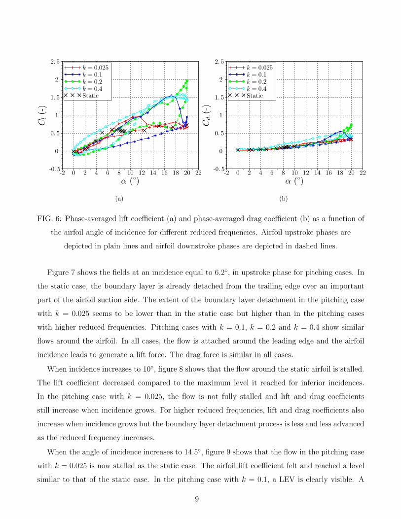
In accordance with previous experimental observations, e.g. [1], the airfoil motion leads to delay

the lift coefficient fall towards higher incidences. The higher the reduced frequency, the higher the

7

(a) Static (b) Pitching, k = 0.025 (c) Pitching, k = 0.1

(d) Pitching, k = 0.2 (e) Pitching, k = 0.4

FIG. 5: Q-criterion isosurface colored by non-dimensional vorticity magnitude, ωc/V0, on the

airfoil suction side at an incidence α ≈ 15◦. Static and pitching cases, upstroke part of the

motion for pitching cases.

incidence delay. The lift coefficient falls around α = 12◦ in the pitching case with k = 0.025

whereas it plunges at the end of the airfoil upstroke when k = 0.2. With the highest reduced

frequency k = 0.4, it occurs during the airfoil downstroke. The lift coefficient reaches higher

values in pitching cases than in a static case. However, once the flow is stalled, the lift coefficient

level is similar in all cases. The lift loss at stall in the oscillating cases is therefore higher than

in the static case. Finally, an important hysteresis phenomenon is observed in the pitching cases.

Lift values observed during upstroke phases are higher than those observed in the static case but

become lower in downstroke phases.

Drag coefficient evolutions are similar until a critical incidence for which the drag coefficient of

the pitching cases increases in a more or less significant manner compared to the static case. This

critical incidence depends on the reduced frequency. The higher the reduced frequency value, the

higher this critical incidence. The drag coefficient then falls more or less drastically and reaches

values similar to those of the static case. Similarly the lift coefficient, the drag coefficient evolution

in the pitching cases shows a hysteresis phenomenon.

To link the evolution of the phase-averaged lift and drag coefficient with the flow around the

airfoil, fields of non-dimensional spanwise vorticity are shown on figures 7 to 14.

8

(a) (b)

FIG. 6: Phase-averaged lift coefficient (a) and phase-averaged drag coefficient (b) as a function of

the airfoil angle of incidence for different reduced frequencies. Airfoil upstroke phases are

depicted in plain lines and airfoil downstroke phases are depicted in dashed lines.

Figure 7 shows the fields at an incidence equal to 6.2◦, in upstroke phase for pitching cases. In

the static case, the boundary layer is already detached from the trailing edge over an important

part of the airfoil suction side. The extent of the boundary layer detachment in the pitching case

with k = 0.025 seems to be lower than in the static case but higher than in the pitching cases

with higher reduced frequencies. Pitching cases with k = 0.1, k = 0.2 and k = 0.4 show similar

flows around the airfoil. In all cases, the flow is attached around the leading edge and the airfoil

incidence leads to generate a lift force. The drag force is similar in all cases.

When incidence increases to 10◦, figure 8 shows that the flow around the static airfoil is stalled.

The lift coefficient decreased compared to the maximum level it reached for inferior incidences.

In the pitching case with k = 0.025, the flow is not fully stalled and lift and drag coefficients

still increase when incidence grows. For higher reduced frequencies, lift and drag coefficients also

increase when incidence grows but the boundary layer detachment process is less and less advanced

as the reduced frequency increases.

When the angle of incidence increases to 14.5◦, figure 9 shows that the flow in the pitching case

with k = 0.025 is now stalled as the static case. The airfoil lift coefficient felt and reached a level

similar to that of the static case. In the pitching case with k = 0.1, a LEV is clearly visible. A

9

LEV is also observed in the pitching case with k = 0.2 but it is less developed at this incidence.

It covers a smaller part of the airfoil suction side. In the pitching case with k = 0.4, the very

beginning of the LEV creation is observed at the leading edge vicinity. The lift coefficient still

increases as the incidence grows for pitching cases with k = 0.1, k = 0.2 and k = 0.4. For k = 0.1,

the drag coefficient slope is henceforth higher.

When incidence increases to 15.9◦, figure 10 shows that the LEV generated in the pitching cases

with k = 0.1, k = 0.2 and k = 0.4 develops and extends on a growing area of the airfoil suction

side. The higher the reduced frequency, the less developed is the LEV. Lift and drag coefficients

continue to increase with incidence. For k = 0.2, the drag and the lift coefficient slopes become

higher around this angle of incidence.

We can observe on figure 11 that when the angle of incidence increases to 19.5◦, the flow around

the pitching airfoil with k = 0.1 is now stalled from the suction side, the LEV has been shed into

the wake. Lift and drag coefficients felt. A counter-rotating Trailing Edge Vortex (TEV) is clearly

visible. For pitching cases with k = 0.2 and k = 0.4, LEV still grows along the airfoil suction side.

The LEV development in the case k = 0.2 is still more advanced than in the case k = 0.4 and

covers a larger part of the airfoil. Lift and drag coefficients are closed to their maximum value.

The deceleration of the airfoil close to the maximum angle of incidence seems to cause a slight

temporary decrease of the lift and drag coefficients for the case with k = 0.4. Reached values with

k = 0.2 are higher than those with k = 0.4.

The airfoil then starts its downstroke phase. Figure 12 shows that at an angle of incidence

equal to 18.1◦the flow is now stalled from the pitching airfoil at k = 0.2, the LEV has been shed

into the wake. As previously for k = 0.1 a TEV is also developing. Lift and drag coefficients felt.

For k = 0.4, the LEV is still on the airfoil suction side and continues to grow. Lift coefficient value

remains high and drag coefficient reaches its maximum value.

When the airfoil incidence decreases to 11.6◦, we see on figure 13 that for the case with k = 0.4

the LEV passes over the airfoil suction side and will be shed into the wake. Lift and drag coefficients

decrease but in a smoother manner compared to the other pitching cases.

Finally, when incidence continues to decrease, the flow over the airfoil starts to reattach from

the leading edge to the trailing edge. Figure 14 shows that the progress of the boundary layer

reattachment at a given incidence depends on the reduced frequency. The higher the reduced

frequency, the more delayed is the process.

Lift and drag coefficients gradually recover the values reached during the upstroke phase, al-

10

though it only happens at the beginning of a new cycle for the lift coefficient of the pitching cases

with a reduced frequency greater than 0.1.

According to the present description and in accordance with [3] the incidence delay of the lift

and drag coefficients drop in a pitching airfoil configuration is due to two successive phenomena:

a boundary layer detachment which happens at higher incidences and the initiation and growth of

a LEV after the boundary layer detachment. The rest of the paper is dedicated to the analysis of

these two phenomena.



FIG. 7: Contours of non-dimensional spanwise vorticity, ωZc/V0, at airfoil midplane for a static

airfoil and for airfoils pitching at various reduced frequencies. The angle of incidence is α = 6.2◦

(upstroke phase).

11




airfoil and for airfoils pitching at various reduced frequencies. The angle of incidence is α = 10◦

(upstroke phase).





(upstroke phase).

12





(upstroke phase).





(upstroke phase).

13





(downstroke phase).





(downstroke phase).

14





(downstroke phase).

15

B. Boundary layer detachment

The boundary layer detachment is investigated for the different pitching cases. Figure 15a

shows the incidence for which Cf local becomes negative during the upstroke phase as a function of

the dimensionless position along the airfoil. It therefore represents the evolution of the boundary

layer detachment point along the airfoil suction side. Positions x/c = 0 and x/c = 1 correspond

to the leading edge and the trailing edge, respectively. Cf local being negative during the entire

cycle in the trailing edge vicinity, curves points do not reach x/c = 1. The airfoil area where the

boundary layer is always detached seems to be more important when the reduced frequency is

high. The boundary layer detachment process goes through larger incidence ranges as the reduced

frequency increases and the detachment point reaches the leading edge vicinity at higher incidences

as the reduced frequency increases. Figure 15b shows the incidence for which the boundary layer

detachment point reaches the leading edge vicinity as a function of the reduced frequency. A

rise of the reduced frequency leads to an increase of the incidence for which the boundary layer

detachment point reaches the leading edge vicinity but in a more important manner at low reduced

frequencies than at high reduced frequencies.

After this part dedicated to the boundary layer detachment, the next section aims to investigate

the Leading Edge Vortex.

0.1 0.2 0.3 0.4 0.5 0.6 0.7 0.8

x/c (-)

0

2

4

6

8

10

12

α(◦)

k = 0.025

k = 0.1

k = 0.2

k = 0.4

(a)

0.00 0.05 0.10 0.15 0.20 0.25 0.30 0.35 0.40 0.45

k (-)

7

8

9

10

11

12

α(◦)

(b)

FIG. 15: (a) Position of the boundary layer detachment point as a function of the airfoil angle of

incidence, (b) Angle of incidence for which the boundary layer detachment point reached the

leading edge vicinity as a function of the reduced frequency.

16

C. Initiation, growth and shedding of the Leading Edge Vortex

α = 14,5°

k = 0.2 k = 0.4

α = 15,9°

α = 19,5°

α = 18,1°downstroke

α = 11,6°downstroke

k = 0.1

FIG. 16: Top: Local lift coefficient Cl local as a function of the dimensionless position on the

airfoil suction side and as a function of the incidence with an isovalue line of Cf local ; Bottom:

non-dimensional spanwise vorticity contours at airfoil midplane for several angles of incidence.

Pictures are scaled to observe the LEV influence on the local lift coefficient ; Left column:

k = 0.1 ; Central column: k = 0.2 ; Right column: k = 0.4 ; J : Angle of incidence at the

beginning of the lift coefficient fall.

The present section focuses on the pitching cases where the LEV is clearly observed: k = 0.1,

k = 0.2 and k = 0.4. Top of figure 16 shows the local lift coefficient Cl local as a function of

17

the dimensionless position on the airfoil suction side and as a function of the incidence during

one pitching cycle for each reduced frequency. These colormaps show the evolution of the lift

distribution along the airfoil suction side during a pitching period. At the beginning of the upstroke

phase, the lift is mostly generated at the leading edge vicinity. As the boundary layer detachment

reaches the leading edge vicinity (at α ≈ 9.1◦ for k = 0.1, α ≈ 10.3◦ for k = 0.2 and α ≈ 11.7◦ for

k = 0.4), the high local lift coefficient area progressively extends along the airfoil suction side. The

leading edge contribution to the lift then drops and a peak of local lift coefficient travels along the

airfoil suction side from the leading edge to the trailing edge. Once this peak of local lift coefficient

passed the trailing edge, the local lift coefficient is low over the whole airfoil suction side during the

rest of the pitching period. The angle of incidence at the beginning of the lift coefficient fall has

been reported by a black triangle on Cl local colormaps. It happens at α ≈ 18◦ for k = 0.1, α ≈ 20◦

for k = 0.2 and α ≈ 16.5◦ in downstroke phase for k = 0.4. The increase of the lift coefficient fall

incidence delay with the rise of the reduced frequency is clearly visible on the Cl local colormaps of

figure 16.

The LEV is a strong vortex and generates a friction force oriented towards the airfoil leading

edge. Isolines of Cf local with negative values have been plotted on Cl local colormaps of figure 16 to

detect the LEV in the different pitching cases and their influence on Cl local. The isolines highlight

that the local lift coefficient peaks which travel along the airfoil suction side are generated by the

LEV. As shown for example by Acharya et al. [4] and by Sharma and Poddar [34], a LEV generates

a depression on the airfoil suction side, which leads to a local peak of the pressure coefficient and

as a consequence of the local lift coefficient in the present study. As the LEV is generated at the

leading edge vicinity, grows and convects along the airfoil until its shedding into the wake, the

LEV generates a local lift coefficient peak that travels along the airfoil suction side. The depression

generated by the LEV therefore increases the airfoil lift coefficient, but also increases the airfoil

drag coefficient as shown by figure 6b.

Contours of non-dimensional spanwise vorticity at airfoil midplane are displayed below the

Cl local colormaps of figure 16. The airfoil chord on the contours is scaled to the abscissa of

Cl local colormaps. Five angles of incidence are displayed and dashed lines report the LEV size on

Cl local colormaps. It shows that isolines of Cf local detect only a part of the LEV. The flow over

the airfoil suction side is complex. The principal vortex has a strong circulation and seems to

generate counter-rotating vortices near the airfoil surface. This behaviour have been also observed

experimentally by Mulleners and Raffel [7]. The friction forces produced by the LEV on the airfoil

18

suction side is therefore not only negative.

Dashed lines of figure 16 report the LEV size on the Cl local colormaps to analyse the LEV

influence on the local lift coefficient distribution. The LEV leads to a high level of local lift

coefficient on the surface it extends. For a given angle of incidence, the local lift coefficient

maximum seems to be located under the LEV centre, where the depression generated by the LEV

is the highest. The higher the reduced frequency, the higher the maximum local lift coefficient

generated by the LEV. The LEV grows as the angle of incidence increases which extends the

high local lift coefficient area on the airfoil suction side. The local lift coefficient maximum moves

with the LEV centre. Then, the LEV gradually detaches from the leading edge, travels beyond

the airfoil suction side before being shed into the wake, which leads to the displacement of the

maximum of the local lift coefficient from the leading edge towards the trailing edge. The lift

coefficient drops during the LEV shedding. Right after the shedding of the LEV into the wake,

a surge of local lift coefficient is observed at the trailing edge vicinity. It seems to be due to a

Trailing Edge Vortex (TEV) which is generated from the airfoil pressure side in response to the

shedding of the LEV.

Following the boundary layer detachment, the LEV generation therefore leads to keep a high

level of lift for a more or less important angular range and increases the incidence delay of the lift

and drag coefficients drop.

This study was so far focussed on the LEV development as a function of the airfoil angle of

incidence. The LEV seems to go through the same steps during its development independently

to the reduced frequency but at higher angles of incidence as the reduced frequency increases.

The rest of the study is focussed on the LEV development over time. The development time of

the LEV will be evaluated with ∆t∗ = ∆tV0c

, the dimensionless time passed since the boundary

layer detachment reached the leading edge vicinity. The colormaps on top of figure 17 show for

each reduced frequency the local lift coefficient as a function of ∆t∗ and as a function of the

dimensionless position along the airfoil suction side. The incidence variation ∆α corresponding

to ∆t∗ depends on the reduced frequency and is indicated on the right axis of the colormaps.

Contours of non-dimensional spanwise vorticity for different ∆t∗ have been reported below the

colormaps for each reduced frequency. Corresponding incidence variations have been reported on

each contour.

In the very first moment of the LEV generation, it seems to develop in a similar manner

independently of the reduced frequency. The LEV occupies the same surface on the airfoil suction

19

side, although the vortex is higher as the reduced frequency increases. The evolution of Cl local

over time is similar for the three pitching cases, although it differs on its amplitude.

Contours of non-dimensional spanwise vorticity of figure 17 show that at ∆t∗ = 3.1, the pitching

airfoil with k = 0.4 is already in downstroke phase which seems to hurried the LEV detachment

from the airfoil suction side. The LEV led to keep a high lift coefficient on an angular range ∆αLEV

of slightly less than 12◦. The pitching cases with k = 0.1 and k = 0.2 still are in upstroke phase

and the LEV is still attached to the airfoil.

At ∆t∗ = 3.5, in the pitching case with k = 0.2, the evolution of local lift coefficient distribution

over the airfoil suction side shows that the LEV gradually detaches. The airfoil is at the maximum

angle of incidence. The LEV detachment therefore occurs when the airfoil rotation speed is close

to zero and the angular interval crossed during the LEV detachment is small. The lift and drag

coefficients as a function of incidence thus drop more brutally compared to the pitching case with

k = 0.4, as seen on figure 6. In the pitching case with k = 0.2, the LEV led to keep a high lift

coefficient on an angular range ∆αLEV of approximately 9.7◦.

It is only at ∆t∗ ≈ 5 that the LEV of the pitching case with k = 0.1 is shed into the wake.

It occurs on an angular range where the airfoil rotation speed is higher than for the case k = 0.2

but still small. The lift and drag coefficient drop as a function of incidence remains fairly brutal

(cf. figure 6). Even though the LEV lifetime is the highest in the pitching case with k = 0.1, the

oscillation frequency being the lowest, the LEV generation led to keep a high lift coefficient on the

smallest angular range, approximately equal to 8.8◦.

In summary, in the very first moments of its generation, the LEV seems to develop over the time

in a similar manner independently of the reduced frequency. The LEV is however more intense

and generates higher maximum value of local lift coefficient as the reduced frequency increases.

Its lifetime on the airfoil suction side then depends on the part of the oscillation cycle for which

the LEV initiates. The shedding of the LEV into the wake seems to be hurried by the beginning

of the airfoil downstroke phase. Therefore, the closer to the maximal angle of incidence the LEV

initiates, the lower its lifetime on the airfoil suction side. Figure 18 shows the angular range ∆αLEV

and the time range ∆t∗LEV between the moment for which the boundary layer detachment reached

the leading edge vicinity and the moment for which the lift and drag coefficients fall as a function

of reduced frequency. An increase of the reduced frequency leading to a LEV initiation at higher

angle of incidence, the LEV lifetime reduces as the reduced frequency increases. However, due to

oscillation frequency differences, the angular range crossed during the LEV lifetime extends as the

20

reduced frequency increases. The lift and drag coefficient drop incidence delay related to the LEV

is therefore more important as the reduced frequency increases.

The pitching case with k = 0.2 produces the highest maximum value of lift coefficient. In the

pitching case with k = 0.1, the LEV initiates early and is shed on the wake before the airfoil

reached the maximal angle of incidence. In the pitching case with k = 0.4, the LEV initiates late

and is not fully developed when the airfoil reaches the maximal angle of incidence. It seems that

in the reduced frequency range investigated it exists an optimal reduced frequency which leads to

the highest maximal value of lift coefficient, corresponding to an optimal LEV generation.

V. CONCLUSIONS

In the present study, Large Eddy Simulations have been performed on a pitching NACA0012

airfoil. The aim of this study was to better understand the reduced frequency influence on the

dynamic stall phenomenon. A local lift coefficient and a local quantity related to the friction on

the airfoil surface have been introduced to analyse the flow influence on the airfoil suction side.

The stall of the flow around an airfoil is delayed in a pitching airfoil compared to a static

case. This incidence delay has been divided into two main phases: a delay in the boundary layer

detachment and the initiation and growth of a Leading Edge Vortex (LEV) which leads to keep a

high level of lift.

A rise of the reduced frequency increases the incidence delay related to the boundary layer

detachment. This increase of the incidence delay seems to be more pronounced if low reduced

frequencies are considered.

The LEV initiates at higher angle of incidence as the reduced frequency increases. At its be-

ginning, the LEV development over time does not seem to be influenced by the reduced frequency,

even though a high reduced frequency leads to a more intense LEV and generates higher max-

imum value of local lift coefficient. However, the LEV lifetime over the airfoil suction side and

consequently the time interval for which a high level of lift is kept could be shortened when the

airfoil is close to the downstroke phase. The LEV lifetime and the lift and drag coefficient stall

incidence delay therefore depends on the part of the oscillation cycle for which the LEV initiates.

An increase of the reduced frequency leading to a LEV initiation at higher angle of incidence, the

LEV lifetime reduces as the reduced frequency increases. However, as the oscillation frequency

increases, the angular range crossed during the LEV lifetime extends as the reduced frequency

increases. The lift and drag coefficient drop incidence delay related to the LEV is therefore more

21

important as the reduced frequency increases. The incidence delay related to the LEV dominates

the incidence delay related to the boundary layer detachment for all tested reduced frequencies.

ACKNOWLEDGMENTS

This work has been supported by the Hydrofluv Project, a Research Program piloted by Hydro-

quest. Vincent Moureau and Ghislain Lartigue from the CORIA lab, and the SUCCESS scientific

group are acknowledged for providing the YALES2 code. Computations presented in this paper

were performed using HPC resources from GENCI-IDRIS (Grant No. 2012-020611) and CIMENT

infrastructure (supported by CPER07 13 CIRA and ANR-10-EQPX-29-01).

[1] W.J. McCroskey. The phenomenon of dynamic stall. Technical report, DTIC Document, 1981.

[2] L.W. Carr. Progress in analysis and prediction of dynamic stall. Journal of aircraft, 25(1):6–17,

1988.

[3] T.C. Corke and F.O. Thomas. Dynamic stall in pitching airfoils: aerodynamic damping and com-

pressibility effects. Annual Review of Fluid Mechanics, 47:479–505, 2015.

[4] M. Acharya and M.H. Metwally. Unsteady pressure field and vorticity production over a pitching

airfoil. AIAA journal, 30(2):403–411, 1992.

[5] T. Lee and P. Gerontakos. Investigation of flow over an oscillating airfoil. Journal of Fluid Mechanics,

512:313–341, 2004.

[6] K. Mulleners and M. Raffel. The onset of dynamic stall revisited. Experiments in fluids, 52(3):779–

793, 2012.

[7] K. Mulleners and M. Raffel. Dynamic stall development. Experiments in fluids, 54(2):1469, 2013.

[8] D.E. Rival, J. Kriegseis, P. Schaub, A. Widmann, and C. Tropea. Characteristic length scales for

vortex detachment on plunging profiles with varying leading-edge geometry. Experiments in fluids,

55(1):1660, 2014.

[9] A. Widmann and C. Tropea. Parameters influencing vortex growth and detachment on unsteady

aerodynamic profiles. Journal of Fluid Mechanics, 773:432–459, 2015.

[10] J.G. Leishman and T.S. Beddoes. A semi-empirical model for dynamic stall. Journal of the American

Helicopter society, 34(3):3–17, 1989.

[11] S. Wang, D.B. Ingham, L. Ma, M. Pourkashanian, and Z. Tao. Numerical investigations on dynamic

22

stall of low reynolds number flow around oscillating airfoils. Computers & Fluids, 39(9):1529–1541,

2010.

[12] P. Wernert, W. Geissler, M. Raffel, and J. Kompenhans. Experimental and numerical investigations

of dynamic stall on a pitching airfoil. AIAA journal, 34(5):982–989, 1996.

[13] G. Martinat, M. Braza, Y. Hoarau, and G. Harran. Turbulence modelling of the flow past a pitching

naca0012 airfoil at 105 and 106 reynolds numbers. Journal of Fluids and Structures, 24(8):1294–1303,

2008.

[14] E. Berton, C. Allain, D. Favier, and C. Maresca. Experimental methods for subsonic flow measure-

ments. Notes on numerical fluid mechanics and multidisciplinary design, 81:97–104, 2002.

[15] K.W. McAlister, L.W. Carr, and W.J. McCroskey. Dynamic stall experiments on the naca 0012

airfoil. Technical report, 1978.

[16] M. Sanchez-Rocha, M. Kirtas, and S. Menon. Zonal hybrid rans-les method for static and oscillating

airfoils and wings. AIAA paper, 1256:2006, 2006.

[17] P.R. Spalart, S. Deck, M.L. Shur, K.D. Squires, M.K. Strelets, and A. Travin. A new version of

detached-eddy simulation, resistant to ambiguous grid densities. Theoretical and computational fluid

dynamics, 20(3):181–195, 2006.

[18] R.A. Piziali. 2-d and 3-d oscillating wing aerodynamics for a range of angles of attack including stall.

Technical report, 1994.

[19] M. Rahromostaqim, A. Posa, and E. Balaras. Numerical investigation of the performance of pitching

airfoils at high amplitudes. AIAA Journal, pages 2221–2232, 2016.

[20] C.S. Peskin. The immersed boundary method. Acta numerica, 11:479–517, 2002.

[21] A.W. Mackowski and C.H.K. Williamson. Direct measurement of thrust and efficiency of an airfoil

undergoing pure pitching. Journal of Fluid Mechanics, 765:524–543, 2015.

[22] D. Garmann and M. Visbal. Implicit les computations for a rapidly pitching plate. AIAA Paper

AIAA-2010-4282, AIAA, 2010.

[23] W.J. McCroskey, K.W. McAlister, L.W. Carr, S.L. Pucci, O. Lambert, and R.F. Indergrand. Dy-

namic stall on advanced airfoil sections. Journal of the American Helicopter Society, 26(3):40–50,

1981.

[24] L.W. Carr, K.W. McAlister, and W.J. McCroskey. Analysis of the development of dynamic stall

based on oscillating airfoil experiments. Technical report, 1977.

[25] V. Moureau, P. Domingo, and L. Vervisch. Design of a massively parallel cfd code for complex

23

geometries. Comptes Rendus Mecanique, 339(2):141–148, 2011.

[26] A.J. Chorin. Numerical solution of the navier-stokes equations. Mathematics of computation,

22(104):745–762, 1968.

[27] M. Malandain, N. Maheu, and V. Moureau. Optimization of the deflated conjugate gradient algorithm

for the solving of elliptic equations on massively parallel machines. Journal of Computational Physics,

238:32–47, 2013.

[28] V. Moureau, P. Domingo, and L. Vervisch. From large-eddy simulation to direct numerical simula-

tion of a lean premixed swirl flame: Filtered laminar flame-pdf modeling. Combustion and Flame,

158(7):1340–1357, 2011.

[29] L. Guedot, G. Lartigue, and V. Moureau. Design of implicit high-order filters on unstructured grids

for the identification of large-scale features in large-eddy simulation and application to a swirl burner.

Physics of Fluids (1994-present), 27(4):045107, 2015.

[30] N. Odier, G. Balarac, C. Corre, and V. Moureau. Numerical study of a flapping liquid sheet sheared

by a high-speed stream. International Journal of Multiphase Flow, 77:196–208, 2015.

[31] M. Kraushaar. Application of the compressible and low-Mach number approaches to Large-Eddy Sim-

ulation of turbulent flows in aero-engines. PhD thesis, Institut National Polytechnique de Toulouse-

INPT, 2011.

[32] M. Germano, U. Piomelli, P. Moin, and W.H. Cabot. A dynamic subgrid-scale eddy viscosity model.

Physics of Fluids A: Fluid Dynamics (1989-1993), 3(7):1760–1765, 1991.

[33] J.C.R. Hunt, A.A. Wray, and P. Moin. Eddies, streams, and convergence zones in turbulent flows.

1988.

[34] D.M. Sharma and K. Poddar. Investigation of dynamic stall characteristics for flow past an oscillat-

ing airfoil at various reduced frequencies by simultaneous piv and surface pressure measurements. In

PIV13; 10th International Symposium on Particle Image Velocimetry, Delft, The Netherlands, July

1-3, 2013. Delft University of Technology, Faculty of Mechanical, Maritime and Materials Engineer-

ing, and Faculty of Aerospace Engineering, 2013.

24

Δt* = 1,2

k = 0.1 k = 0.2 k = 0.4

Δt* = 2

Δt* = 2,4

Δt* = 3,1

Δt* = 4,7

Δα = 2.5° Δα = 4.2° Δα = 7.2°

Δα = 4° Δα = 6.8° Δα = 8.2°

Δα = 4.7° Δα = 7.8° Δα = 9.4°

Δα = 6.1° Δα = 9.2° Δα = 13.8°

Δα = 8.5° Δα = 10.2° Δα = 25.4°

FIG. 17: Top: Local lift coefficient as a function of dimensionless position along the airfoil

suction side and as a function of dimensionless passed time since the boundary layer detachment

reaches the leading edge vicinity. Corresponding incidence variation is indicated on the right axis

of each colormap ; Bottom: non-dimensional spanwise vorticity contours at airfoil midplane for

several passed time since the boundary layer detachment reaches the leading edge vicinity. The

corresponding incidence variation is indicated on each contour ; Left column: k = 0.1 ; Central

column: k = 0.2 ; Right column: k = 0.4 ; J : Angle of incidence at the beginning of the lift

coefficient fall.

25

0.0 0.1 0.2 0.3 0.4 0.5

k (-)

8.5

9.0

9.5

10.0

10.5

11.0

11.5

12.0

12.5

13.0

∆αLEV(◦)

∆αLEV

2.5

3.0

3.5

4.0

4.5

5.0

5.5

6.0

∆t∗ L

EV(-)

∆t∗LEV

FIG. 18: Angular range ∆αLEV and dimensionless time range ∆t∗LEV between the moment for

which the boundary layer detachment reached the leading edge vicinity and the moment for

which the lift and drag coefficients fall as a function of reduced frequency.

26

Large Eddy Simulations on a pitching airfoil: Analysis of ...

Documents

Transcript of Large Eddy Simulations on a pitching airfoil: Analysis of ...