LARGE DEVIATION PRINCIPLE FOR SUM OF SUBEXPONENTIAL...

jacopo cattaneo

L A R G E D E V I AT I O N P R I N C I P L E F O R S U M O FS U B E X P O N E N T I A L VA R I A B L E S : T H E 1 D M AT C H I N G

P R O B L E M

L AU R E A M A G I S T R A L E I N F I S I C A

L A R G E D E V I AT I O N P R I N C I P L E F O R S U M O FS U B E X P O N E N T I A L VA R I A B L E S : T H E 1 D M AT C H I N G P R O B L E M

jacopo cattaneo

thesis advisor

dr . sergio caracciolo

thesis co-advisors

mauro pastore , andrea di gioacchino

April 4th, 2019

Jacopo Cattaneo: Large deviation principle for sum of subexponential vari-ables: the 1D matching problem, , c⃝ April 4th, 2019

To the loving memory of my grandparents.

A B S T R A C T

Large deviation theory connects different areas of physical interest,being able to justify the average properties of statistical ensembleswhile characterizing rare events and probabilities of extreme values.

In this work we focused on its application to the cost function of therandom euclidean matching problem (REMP) on a compact interval.This is a well known toy-model belonging to the family of disorderedspin-glass systems and optimization problems. In our case the costfunction is given by the distance of two matched points (spacing) raisedto some power p > 1.

In here we present the main results obtained in the case of indepen-dent, identically distributed, spacings, providing a precise asymptoticexpression for the probability distribution of the cost function. In par-ticular, we found two threshold sequences depending on the numberof random variables n and the power p, which define different regionswhere different behaviors can be observed. On one hand, we showthat in a region close to the expected value, deviations from the meanare exponentially suppressed in the number of spacings, which istypical. On the other hand, in a broader region, probability of rareevents is less than exponentially dumped, making extreme values notso unlikely.

Moreover, even when correlations between spacings induced bythe distance are taken into account, we show that the distributionof the average optimal cost in the REMP is asymptotically normallydistributed in the region predicted by the central limit theorem. Weshow this region can be extended on a broader interval, defining amoderate large deviation principle in a range limited, as before, by asuitable threshold sequence.

Both results are supported by numerical simulations. These wereobtained from direct sampling the distribution of the spacings andthus evaluating the cost function for different choices of p.

vii

A C K N O W L E D G M E N T S

I would like to thank everybody who, directly and indirectly, partici-pated to this work.

First of all I would like to thank my thesis advisor, professor SergioCaracciolo, a source of inspirational motivation. A big thanks goes tomy co-advisors, Andrea Di Gioacchino and especially Mauro Pastore,that helped and supported me during the whole project.

A big thank goes to my parents, my family and my loved ones.To all of my friends of Nuova Zelanda, to the Tombino gang, to the oldand new acquaintances, to all of you a huge hug for having enduredme. I know it was not that easy.

To everybody who would have preferred to see his name cited here,I’m happy to disappoint them. I’m joking, I just had no time.

Cheers!

ix

C O N T E N T S

i large deviation principle and the one dimen-sional euclidean matching problem

1 introduction to the large deviation theory 3

1.1 Why a large deviation theory 3

1.2 Basic elements of probability theory 4

1.3 From small to large deviations 5

1.3.1 A combinatorial example 6

1.4 Some useful results in large deviation theory 7

1.5 Large deviations in statistical mechanics 11

2 the one dimensional random euclidean match-ing problem 13

2.1 Disordered Systems 13

2.1.1 What is disorder 13

2.1.2 Large deviations in glassy systems 15

2.2 Random optimization problems 15

2.2.1 The matching problem 16

2.3 The random Euclidean matching problem on an inter-val 18

2.3.1 Probability distribution of random uniform spac-ings on an interval 19

3 a large deviation principle for the independent

case 25

3.1 A simple case: the sample mean of exponential randomvariables 25

3.2 The case of REMP 26

3.3 Subexponential distributions 29

3.3.1 Large deviations for sample mean of stretchedexponential random variables 32

3.4 The LDP for sum of powers of IID exponential RVs 33

3.5 Numerical simulations 35

3.5.1 Direct sampling method 35

3.5.2 Simulation results 37

4 an ldp for the average cost of remp 41

4.1 The central limit theorem for dependent variables 41

4.1.1 The fundamental formula 41

4.1.2 The Gaussian regime 42

4.2 The extension to large deviations 44

4.2.1 The Gaussian moderate deviations 44

4.2.2 Large deviations for the tail probability 46

4.3 Numerical simulations 47

4.4 Conclusion and outcomes 47

xi

xii contents

ii appendix

a the legendre-fenchel transform 53

a.1 Definition and first properties 53

a.2 Theory of Legendre-Fenchel transform 54

bibliography 59

Part I

L A R G E D E V I AT I O N P R I N C I P L E A N D T H E O N ED I M E N S I O N A L E U C L I D E A N M AT C H I N G

P R O B L E M

1I N T R O D U C T I O N T O T H E L A R G E D E V I AT I O NT H E O RY

In this chapter we want to give some fundamental notions of largedeviation theory and its applications in physics. We want to givesome sense of what a large deviation is by a simple introduction toprobability theory and collecting the fundamental results in this field.A simple application to statistical mechanics is given at the end of thechapter which tries to justify the physical interest of the topic. A goodintroduction to this topic can be found in the book of R. Ellis [11] andin the Lecture Notes in Physics book series by Springer [40]

1.1 why a large deviation theory

Describing the physical properties of macroscopic bodies via the com-putation of (ensemble) averages was the main focus of statisticalmechanics at its early stage. As a matter of fact, as macroscopic bodiesare made of a huge number of particles, fluctuations were expected tobe too small to be actually observable. Broadly speaking, we can saythat the theoretical basis of statistical descriptions was guaranteed bythe law of large numbers.On the other hand, whenever physicists calculate an entropy functionor a free energy function, large deviation theory is at play. Indeed,large deviation theory is almost always involved when one studiesthe properties of many-particle systems, be they equilibrium or nonequilibrium systems. It explains, for example, why the entropy andfree energy functions are mutually connected by a Legendre transform,and so provides an explanation of the appearance of this transform inthermodynamics. Large deviation theory also explains why equilib-rium states can be calculated via the extremum principles that are the(canonical) minimum free energy principle and the (microcanonical)maximum entropy principle.

The earliest origins of large deviation theory lie in the work ofBoltzmann on entropy in the 1870ies [34] and Cramér’s Theorem from1938 [7, 8]. A unifying mathematical formalism was only developedstarting with Varadhan’s definition of a large deviation principle (LDP)in 1966 [37, 38].

Basically, large deviation theory centers around the observation thatsuitable functions f of large numbers of random variables (X1, . . . ,Xn)

often have the property that, for n ≫ 1,

Pr (f(X1, . . . ,Xn) ∈ dx) ∼ e−anI(x) dx , (1.1)

3

4 introduction to the large deviation theory

where an is a suitable sequence such that limn→∞ an = ∞ (in mostcases simply an = n). In other words, LDP states that the probabilitythat f(X1, . . . ,Xn) takes values near a point x decays exponentiallyfast, with speed an, and rate function I.

Large deviation theory has two different aspects. On the one hand,there is the question of how to formalize the intuitive formula (1.1).This leads to the already mentioned definition of large deviationprinciples and involves quite a bit of measure theory and real analysis.

On the other hand, there is a much richer and much more importantside of large deviation theory, which tries to identify rate functionsI for various functions f and study their properties. This part of thetheory is as rich as the branch of probability theory that tries to provelimit theorems for functions of large numbers of random variables,and has many relations to the latter.

1.2 basic elements of probability theory

We start our study of large deviation theory by considering f as a sumof real random variables (RV for short) having the form

Sn =1

n

n∑i=0

Xi . (1.2)

Such a sum is often referred to in mathematics or statistics as a samplemean. Three basic questions naturally arise when n is very large:

• The behavior of the sample mean Sn , the possible convergenceto an asymptotic value and its dependence on the sequence;

• The statistics of small fluctuations of Sn around ⟨Sn⟩, i.e. ofδSn = Sn − ⟨Sn⟩, when |δSn| is small;

• The statistical properties of rare events when such fluctuationsare large.

The answer to the first question, in the simple case of sequences(X1, . . . ,Xn) of independent and identically distributed (IID for short)random variables with expected value µ and with finite variance,comes form the law of large numbers (LLN) which states the empiricalaverage gets closer and closer to the expected value µ = ⟨Xi⟩, when n

is large:

limn→∞ Pr (|δSn| < ϵ) = 1 . (1.3)

The second issue is addressed by the central limit theorem (CLT). Forinstance, in the case of IID RV with expected value µ and finite varianceσ2, the CLT describes the statistics of small fluctuations, |δSn| .

1.3 from small to large deviations 5

O(σ/√n), around the mean value when n is very large. Roughly

speaking, the CLT proves that, in the limit n ≫ 1, the quantity

Zn =1

σ√n

n∑i=0

(Xi − µ)

is normally distributed, meaning that

pZn(z) ∼

1√2π

e−z2/2 (1.4)

independently of the distribution of the random variables. Undersuitable hypothesis the theorem can be extended to dependent (weaklycorrelated) variables.

Finally, the last point is the subject of large deviation theory which,roughly, states that in the limit n ≫ 1

pSn(s) ∼ e−anI(s) , (1.5)

or, equivalently,

limn→∞ 1

anlogpSn

(s) = −I(s) . (1.6)

Unlike the central limit theorem result with the universal limit prob-ability density (1.4), the detailed functional dependence of I(s) – theCramér’s or rate function – and the speed an depends on the probabilitydistribution of p(X1, . . . ,Xn). However, I(s) possesses some generalproperties: it is zero for s = ⟨Sn⟩ and positive otherwise, moreover– when the variables are independent (or weakly correlated) – it isa convex function. A motivation of this last statement is providedin Appendix A. For a complete study of the properties of the ratefunction we refer to [36, 39]. For sake of simplicity in the following wewill assume an = n, which is common in most simple cases.

1.3 from small to large deviations

An LDP for a random variable, say Sn again, gives us a lot of infor-mation about its distribution. The fact that the behavior of pSn

(s) isdominated for large n by a decaying exponential means that the exactdistribution of Sn can be written as

pSn(s) = e−nI(s)+o(n)

with o(n) a sublinear correction in n. By taking the limit

limn→∞ 1

nlogpSn

(s) = I(s) + limn→∞ o(n)

n= I(s)

which retains only the dominant exponential term of the limitingdistribution and neglects the others. For this reason, large deviation


theory is often said to be concerned with estimates of probabilities onthe logarithmic scale.

Thus it should be clear that probability is exponentially suppressedin n anywhere the rate function I(s) is non-vanishing. Moreover, weknow that pSn

(s) concentrates on certain points which are the typicalvalues of the sample mean Sn in the large n limit. These pointscorrespond to the zeroes of the rate function I(s) and it can be shownto be related mathematically to the LLN. Indeed, an LDP alwaysimplies some form of LLN.

Often it is not enough to know that Sn converges in probability tosome values and we may also want to determine the likelihood thatSn takes a value away but close to its typical value. Let s0 be one ofthis values and assume that I(s) admits a Taylor series around s0, then

I(s) = I(s0)+ I ′(s0)(s− s0)+I ′′(s0)

2(s− s0)

2+o((s− s0)

2)

. (1.7)

Since s0 is a zero of I(s) the first two terms vanish and we are leftwith a law of small deviations of Sn around its typical value

pSn(s) ∼ e−n

I ′′(s0)2 (s−s0)

2

.

and in this sense, large deviation theory contains the CLT. At the sametime, large deviation theory can be seen as an extension of the latterbecause it gives information not only about the small deviations butalso about large deviations far away from its typical value(s).

1.3.1 A combinatorial example

A natural way to introduce the large deviation theory and show itsdeep relation with the concept of entropy is to perform a combinatorialcomputation. We will consider the simple example of a sequence ofindependent unfair-coin tosses. Denoting with Xi the result of thei-th toss, the possible outcomes are head (+1) with probability π ortail (−1) with probability 1− π. Let Sn be the sample mean of suchvariables, we are now interested in formulating an LDP for the RV Sn.

Actually, the probability of the sample mean taking a specific valuecan be explicitly computed: in the sequence of n tosses of the coin theways k heads can occur is given by the binomial coefficient(

n

k

)=

n!k! (n− k)!

.

Thus, we have for the probability of the sample mean

Pr(Sn =

2k

n− 1

)=

n!k! (n− k)!

πk(1− π)n−k , (1.8)

that is the binomial distribution.

1.4 some useful results in large deviation theory 7

Since we are interested in the asymptotic expression in the large n

limit, both the number of heads and the number of tails will diverge.Thus, by setting

k = pn ,

n− k = (1− p)n ,

and using Stirling approximation of the factorial, the probability in(1.8) will take the form

Pr (Sn = 2p− 1) ∼ e−nIπ(p) , (1.9)

where

Iπ(p) = p logp

π+ (1− p) log

1− p

1− π(1.10)

is the rate function of the probability distribution. We can noticeIπ(π) = 0, meaning the only value for which the probability is nonvanishing is the expected value of the sample mean. Actually, the CLTcan be recovered by a Taylor expansion at p = π, that is

Iπ(p) =1

2

(p− π)2

π(1− π)+ o

((p− π)2

). (1.11)

From the above computation we understand that it is possible to gobeyond the CLT, and to estimate the statistical features of extreme (ortail) events, as the number of observations n grows without bounds.

1.4 some useful results in large deviation theory

The first approximation we can have on the distribution comes fromthe Markov’s inequality, that gives an upper bound for the probabilitythat a non-negative function of a random variable is greater than orequal to some positive constant. It relates probabilities to expectations,and provide bounds for the cumulative distribution function of arandom variable. It is obtained by noting that, for any non-negativeRV X with probability density function (PDF for short) p(x), it holds

⟨X⟩ =∫∞0

dx xp(x) =

∫a0

dx xp(x) +

∫∞a

dx xp(x)

>∫∞a

dx xp(x) > a

∫∞a

dxp(x) = aPr(X > a) ,

for any positive a. Therefore we have

Pr(X > a) 6⟨X⟩a

(1.12)

A direct consequence of Markov’s inequality is the Chernoff bound[6], that gives exponentially decreasing bounds on tail distributions


of sums of independent random variables. This is simply obtained byapplying (1.12) to the RV etX,

Pr(X > a) = Pr(etX > eta

)6

⟨etX⟩

eta,

that holds for any t > 0. Now, let X = Sn be the sample mean of IIDRVs: by recalling that

p(n)(X1, . . . ,Xn) =

n∏i=1

p(1)(Xi) , (1.13)

then it holds

Pr(Sn > s) = Pr

(n∑

i=0

Xi > ns

)= Pr

(et

∑ni=0 Xi > etns

)6

(⟨etX⟩

ets

)n

6

(mint>0

[e−ts

⟨etX⟩])n

.

Thus, in terms of large deviation theory,

limn→∞ 1

nlog Pr(Sn > s) 6 − sup

t>0

[ts− logM(t)] (1.14)

where M(t) ≡⟨etX⟩

is the moment generating function (MGF) of thevariable X.A similar Chernoff bound can be obtained for the complementaryprobability: namely, for any t 6 0, we have

Pr(Sn 6 s) = Pr(et

∑ni=0 Xi > etns

)6

(mint60

[e−ts

⟨etX⟩])n

,

and thus

limn→∞ 1

nlog Pr(Sn 6 s) 6 − sup

t60

[ts− logM(t)] . (1.15)

The main result of large deviation theory that is widely used toobtain LDPs is called the Gärtner–Ellis Theorem (GE Theorem) [12,14]. Let

K(λ) = limn→∞ 1

nlog⟨enλfn

⟩fn

(1.16)

be the scaled cumulant generating function (SCGF) for some real RV fnparametrized by n, where⟨

enλfn⟩fn

=

∫Pr (fn ∈ dx) enλx . (1.17)

In the following we will omit the subscript on which probabilitymeasure the expectation value is taken unless it is essential for un-derstanding. The GE Theorem states that if K(λ) exists ∀λ ∈ R and isdifferentiable then fn satisfies a LDP

Pr (fn ∈ dx) ∼ e−nI(x) dx , (1.18)

1.4 some useful results in large deviation theory 9

with rate function I(x) given by

I(x) = supλ

[λx−K(λ)] . (1.19)

The transform defined by the supremum is an extension of the Leg-endre transform referred to as the Legendre–Fenchel transform (LFT forshort). We refer to Appendix A for a more in-depth discussion.

The GE Theorem thus states in words that, when the SCGF K(λ) isdifferentiable, then fn obeys a large deviation principle with a ratefunction I(x) given by the LFT of K(λ).The SCGF has some interesting properties: since the probability mea-sure is normalized K(0) = 0 and, for m ∈ N, it holds

K(m)(0) =∂m

∂λmK(λ)

λ=0

= limn→∞ 1

n

∂m

∂λmlog⟨enλfn

⟩λ=0

= κm

where κm is the m-th cumulant of fn. In particular, the first twocumulants correspond to

κ1 = limn→∞ ⟨fn⟩fn = µ

κ2 = limn→∞n

(⟨f2n⟩− ⟨fn⟩2

)= lim

n→∞nvar(fn) .

The importance of the GE Theorem is to be able to calculate theSCGF without knowing the exact form of pfn(x). Conversely, theasymptotic expression of the distribution pfn(x) can be retrieved ex-actly with this theorem, by the evaluation of the rate function itself.

The rigorous proof of the GE Theorem is too technical to be pre-sented here. However, there is a way to justify this result by derivingin a heuristic way another result known as Varadhan’s Theorem. Thelatter theorem is concerned with the evaluation of a functional expec-tation of the form

Wn [g] =⟨eng(fn)

⟩=

∫dxpfn(x)e

ng(x) (1.20)

with g some function of the real RV fn. Assuming fn satisfies a LDPwith rate function I(x), then we can write

Wn [g] ∼

∫dx en[g(x)−I(x)]

∼ en supx[g(x)−I(x)]

where the last equality follows from the saddle-point approximationor Laplace approximation, and it is justified in the context of largedeviation theory because the corrections to this approximation are


subexponential in n, as are those of the LDP. By defining the followingfunctional

K[g] = limn→∞ 1

nlogWn[g] ,

using a limit similar to the limit defining the LDP, we then obtain

K[g] = supx

[g(x) − I(x)] . (1.21)

The result above is what is referred to as Varadhan’s Theorem [37],which proved this result for a wide class of RV.

To connect Varadhan’s Theorem with the GE Theorem we considerthe special case g(s) = λs with λ ∈ R. Then equation in (1.21) becomes

K(λ) = supx

[λx− I(x)] , (1.22)

which is the same function defined in (1.16).Thus it is clear that if Sn satisfies a LDP with rate function I(s), thenthe SCGF K(λ) is the LFT of I(s).

This heuristic derivation illustrates two important points about largedeviation theory. The first is that LFTs appear into this theory as anatural consequence of the saddle point approximation. The secondis that the Gärtner–Ellis Theorem is essentially a consequence of thelarge deviation principle combined with Laplace’s approximation.

To complete this presentation of known results it is useful to have alook at the application of GE Theorem in the special case of the samplemean of a set of IID RV (X1, . . . ,Xn). Namely, by taking fn = Sn as in(1.2) and by recalling that

p(n)(X1, . . . ,Xn) =

n∏i=1

p(1)(Xi) ,

we can write for the SCGF

KSn(λ) = lim

n→∞ 1

nlog⟨enλSn

⟩n

= limn→∞ 1

nlog

[n∏

i=1

⟨eλXi

⟩1

]= log

⟨eλX

⟩1

. (1.23)

As a result the SCGF KSnis simply derived by the cumulant generating

function of the single RV X and the LDP for Sn is retrieved by takingthe LFT just as in (1.19). This result goes under the name of Cramér’sTheorem and plays a central role in determining a large deviationprinciple for the sample mean of different RV.Note that the differentiability condition of the GE Theorem need not bechecked for IID sample means because the moment generating function

1.5 large deviations in statistical mechanics 11

(MGF) or Laplace transform⟨eλX

⟩1

of a RV is always real analytic whenit exists ∀λ ∈ R. On the other hand, the existence of the MGF on thepositive real axis (usually referred to as Cramér’s condition) must not betaken for granted and sometimes more refined tools may be necessaryto establish an LDP.

1.5 large deviations in statistical mechanics

As it has been said the mathematical basis for the notion of thermo-dynamic behavior is the LLN. The idea is that the outcomes of amacrostate, say Mn(ω), involving n particles should concentrate inprobability around certain equilibrium values despite the fact that theparticles’ microstate is modeled by a random variable ω taking valuesin the phase space Λn. Large deviation theory enters this picture bynoting that, in many cases, the outcomes of the macrostate are ruled bya large deviation principle, and that, in these cases, the concentrationof probability measure pMn

around these equilibrium values is expo-nentially fast in the large n limit. Consequently, all that is needed todescribe the state of a large many-particle system at the macroscopiclevel is to know the equilibrium values of Mn which correspond tothe global minima of the rate function governing the fluctuations.

Let us consider the microcanonical ensemble, that is a closed systemwith constant energy. We can start by writing the probability that theenergy ϵn sits in a range dϵ in terms of the probability measure of themicrostates

Pr(ϵn ∈ dϵ) =

∫Λn

δ (ϵn(ω) − ϵ)Pr(dω) .

By taking the uniform measure Pr(dω) = dω/|Λ|n it appears thatPr(ϵn ∈ dϵ) is proportional to the volume in the phase space occupiedby microstates which satisfy ϵn(ω) = ϵ, namely

Ωϵn(ϵ) =

∫Λn

δ (ϵn(ω) − ϵ)dω .

Thus, by admitting ϵn satisfies an LDP with rate function I(ϵ), wehave

I(ϵ) = − limn→∞ 1

nlog Pr(ϵn ∈ dϵ) ≡ −s(ϵ)

where

s(ϵ) = limn→∞ 1

nlog

Ωϵn(ϵ)

|Λ|n

is the microcanonical entropy density. Moreover, proportionality betweenPr(ϵn ∈ dϵ) and Ωϵn(ϵ) implies for the SCGF

K(λ) = limn→∞ 1

nlog⟨enλϵn

⟩= − βϕ(β)|β=−λ


where ϕ(β) is the free energy density. More explicitly

ϕ(β) = − limn→∞ 1

βnlogZn(β)

= − limn→∞ 1

βnlog

∫Λn

dωe−nβϵn(ω)

= − limn→∞ 1

βnlog⟨e−nβϵn

⟩.

As a consequence, from Varadhan’s and GE Theorem, we can establishthe relation between ϕ(β) and s(ϵ)

βϕ(β) = infϵ[βϵ+ s(ϵ)] ,

s(ϵ) = − infβ[βϵ−βϕ(β)] ,

that is the entropy and the free energy can be obtained by an LFT.As it may have become clear, LDT is at play each time we are

interested in average properties of statistical ensembles, while account-ing for probability of rare events. In particular, we showed that boththe SCGF and the rate function itself are related to thermodynamicquantities of great physical interest, that is the free energy and entropy.

2T H E O N E D I M E N S I O N A L R A N D O M E U C L I D E A NM AT C H I N G P R O B L E M

2.1 disordered systems

Before we start studying a specific spin-glass model, we need tointroduce a couple of simple concepts, which we will extensively useall along the dissertation. Each of them would deserve much morespace than we can afford: we refer to [5, 24] for a background instatistical mechanics and glassy systems.

2.1.1 What is disorder

As already pointed out in the previous chapter, when we study asystem involving a large number n of observables, we are mainlyinterested in finding the expression of some average properties, that isthe value of a macroscopic measurable quantity.

In the language of statistical mechanics this is usually achieved bythe evaluation of the partition function

Z(β) =∑ω∈S

e−βϵ(ω) , (2.1)

where each microstate ω, in the space of configurations S, is associatedwith the corresponding energy ϵ(ω). This dependence between energyϵ and microstates ω is expressed by the dependence of the energy onthe parameters describing the microstate, that is the Hamiltonian H.From the partition function in (2.1), we can obtain a lot of informationon the average, or typical, values that different quantities of physicalinterest can assume. As an example, the mean energy can be retrievedby a simple derivation of the partition function, that is

E = −∂

∂βlogZ(β) . (2.2)

The simplest way to introduce disorder in any system is consideringsome of the parameters describing the microstate ω as stochasticvariables. There are two main classes of disordered systems: the firstwe are going to discuss are quenched disordered systems. In thesesystems the disorder is explicitly present in the Hamiltonian, typicallyunder the form of random couplings J among the degrees of freedomσ

H = H(J,σ) .

13

14 the one dimensional random euclidean matching problem

The disorder introduced by the set of RVs J is completely specified bytheir probability distribution p(J) which is assumed to be the same foreach different coupling constant in the system. A famous example isthe Edwards-Anderson model [10], described by the Hamiltonian

H = −∑⟨i,j⟩

Jijσiσj ,

where the spins σi = ±1 are the degrees of freedom of the system,and the couplings Jij are Gaussian RVs. This is a finite dimensionalmodel, since the sum is performed over nearest-neighbor spins. Inthis case we say the disorder is quenched, meaning that the set ofRVs J are constant on the time scale over which the the degrees offreedom σ fluctuate. This fact is realized in physical systems where the(microscopic) parameters governing the evolution of the system, thatis the variables on which the Hamiltonian depends on, at sufficientlylow temperatures can be separated into two different classes, slow andfast observables. The difference between the two classes arises fromnoticing that the typical time scale of evolution of an observable (inthis case the couplings Jij) is much larger than the time scale on whichthe spins σi interact. These systems are called spin-glass systemsand an extended literature has been produced around this kind ofproblems [1, 24, 35].

As a matter of fact disorder creates frustration: it becomes impos-sible to satisfy all the couplings at the same time, as it would be ina ferromagnetic system. Formally, a system is said to be frustrated ifthere exists a loop on which the product of the couplings is negative.This can be better understood by looking at a frustrated loop: if wefix an initial spin, and starting from it we try to chain-fix the otherspins one after the other according to the sign of the couplings, we arebound to return to the initial spin and flip it. As a consequence, theenergy of a frustrated loop is not located at its minimum, as it wouldbe if the couplings Jij could explore the whole configurations’ space.

On the other hand, if the time scale of the parameters describing thesystem are of the same magnitude, this implies the time evolution ofall the observables must be taken into account simultaneously whencomputing ensemble averages. Such kind of randomness is usuallyreferred to as annealed disorder. This is often the case of spin-glasssystems at high temperature, where the frustration induced by thedisorder is irrelevant, as the system can visit a lot of different, oftenhigh energy, configurations due to the effect of the entropic force.

In the following we will deal only with quenched disordered sys-tems, that is statistical systems where a bunch of degrees of freedomcannot fluctuate freely and the space of configurations is restricteddue to the specific realization of the parameters.

2.2 random optimization problems 15

2.1.2 Large deviations in glassy systems

In the study of disordered systems nearly all predictions concernthe most likely behavior, but there is also considerable interest indeveloping techniques to compute the probability distribution of rareevents, i. e. the probability of finding systems that have propertiesdifferent from the typical ones. Systems with quenched disorder havebeen studied intensively for the last two decades. Thermodynamicproperties in these systems, such as the free energy, fluctuate fromsample to sample, but not very much: indeed, they are self-averagingif the disorder does not have long range correlations [19]. This meansthat typical values of the free energy density (to name but one quantity)deviate arbitrarily little from a fixed value in the large volume limit.

Because of this, little work has considered large deviations, i. e.the probability of finding a rare sample (realization of the disorder).Indeed it is well known that the probability of large deviations isrelated to the free energy function ϕ(β). Thus we are interested in bigoscillations of this quantity when we try to formulate an LDP for anyobservable in a disordered system. As already discussed in Section 1.5,in LDT the analog of the free energy is the SCGF: this will play acentral role in determining big oscillations from the typical values forthe quantities of interest.

2.2 random optimization problems

Combinatorial optimization is a branch of operational research whichdeals with the problem of optimizing a cost function over a finite setof configurations. Let S be the set of all the possible configurations ω

a system can explore. Then, given a cost function E(ω) ∈ R, we areinterested in finding the optimal configuration ω∗ ∈ S that minimizessuch cost, namely

E(ω∗) = minω∈S

E(ω) .

In terms of statistical systems discussed in the previous section, thecost function E(ω) can be interpreted as the energy of a configuration.In this case the problem of finding the optimal cost corresponds tofind the average energy in the zero temperature limit. More explicitly,the optimal cost is retrieved from (2.2) by simply taking the limit forβ → ∞, that is

E(ω∗) = − limβ→∞ ∂

∂βlogZ(β) .

When considering a random optimization problem we mean a specialkind of optimization problem where the space of configuration S

depends on some random parameters. It is quite clear that in this caseE = E(ω∗), i. e. the set S of possible configurations, will depend on


the particular realization of the set of RVs, which remains fixed forany realization. As a consequence, this kind of systems belong to thebigger family of glassy systems.

We call S an instance of the problem and we are interested in findingthe average properties of the optimal solution. In particular, denotingwith ⟨•⟩ the average over the instances, we could ask what is theaverage minimal cost

⟨E⟩ =⟨

minω∈S

E(ω)

⟩= − lim

β→∞⟨

∂

∂βlogZ(β)

⟩. (2.3)

After the seminal works of Kirkpatrick [18] Orland [30], and Mézardand Parisi [21], random optimization problems have been successfullystudied using statistical physics techniques. The average appearingin the previous equation can be tackled using the celebrated replicatrick, which allowed the derivation of fundamental results for manyrelevant random combinatorial optimization problems, like randommatching problems [21–23, 30] or the traveling salesman problem inits random formulation [20, 30].

Very often the set of the configurations S is described in the modernabstract framework of graph theory. It seems useful to briefly recallsome definitions of this field: an (undirected) graph G is a couple (V ,E)where

• V is the set of vertices of the graph;

• E ⊆ V × V is the set of edges, where e ∈ E is an unordered pairof vertices, namely e = (u, v) ⊂ V , v = u.

The vertices u and v are said to be the ends of the edge e = (u, v)and thus we say the edge e is incident onto both v and u. A graphK = (V ,E) is said to be complete if each pair of vertices are connectedby an edge (i.e. (u, v) ⊂ V ⇔ e = (u, v) ∈ E).With this definitions we are now able to present the main topic of thischapter.

2.2.1 The matching problem

The matching problem is a rather simple system which has similaritieswith spin glasses with finite range interactions [24]. Its applicationsgo from biology [13], to traffic modeling [3, 31], to neural networks[32, 41]. Here we want to define the generic problem in terms of graphtheory and give a hint of the different flavors it can assume.

Given a graph G = (V ,E) a matching µ ⊆ E is a set of edges havingthe property that none of the edges in µ have an end in common.More explicitly, for any e1, e2 ∈ µ, then e1 ∩ e2 = ∅. We say that avertex v ∈ V is matched if there is an edge incident to v in the matching,otherwise the vertex is unmatched.

2.2 random optimization problems 17

Denoting by |µ| the cardinality of µ, we define ν(G) ≡ maxµ|µ| thematching number of G. As a consequence a matching µ is maximum ifthere is no matching of greater cardinality, that is if |µ| = ν(G) . Inparticular, a maximum matching is called perfect if every vertex of Gis matched. Obviously any perfect matching is maximum and thusmaximal and we will denote by M the set of perfect matchings.

Now, we can imagine to assign a cost to each edge in the graph: letwe > 0 be a weight corresponding to the edge e ∈ E in the graph G.Then we can associate to each perfect matching µ ∈ M the total costfunction

E(µ) ≡∑e∈µ

we (2.4)

and the average cost per edge

ε(µ) ≡ E(µ)

ν(G)=

1

ν(G)

∑e∈µ

we . (2.5)

In the weighted matching problem we search for the perfect matchingµ such that the total cost in (2.4) is minimized, that is the optimalmatching µ∗ is such that

E(µ∗) = minµ∈M

E(µ) . (2.6)

In the following we will deal with random matching problems,where the costs wee∈E are RVs. In this case, the average propertiesof the optimal solution are of a certain interest, and in particular thetypical optimal cost, ⟨E⟩ = ⟨minµ E(µ)⟩. The simplest way we canimagine to introduce randomness in the problem is to consider theweights as IID RVs. A number of rigorous result were obtained in thismean field theory, starting from the work of Parisi and Mézard [21].

In this work, we will focus on the random Euclidean matching prob-lem (REMP), where the graph G is supposed to be embedded in ad-dimensional Euclidean domain Λ ⊆ Rd through an embeddingfunction Φ, in such a way that each vertex v ∈ V of the graph isassociated to a random Euclidean point v ↦→ Φ(v) ∈ Λ. In this casethe random weights we associated to each edge e = (u, v) ∈ E willbe some function of the distance of the corresponding points in Λ,namely

we = f (∥Φ(u) −Φ(v)∥) .

REMPs are usually more difficult to investigate than the purely ran-dom case of we IID RVs, due to the presence of Euclidean correlationsamong the weights. This induces a non-trivial dependence betweenthe RVs, that result in the problem being more complex to investigate.


2.3 the random euclidean matching problem on an in-terval

In the following we will restrict ourselves to a specific toy model inone dimension, that is the random Euclidean matching problem. Herewe refer to the work of Caracciolo, D’Achille, Sicuro [4], that obtaineda number of results for this system.

We will focus only on the case in which G = K2n is a com-plete graphs with 2n vertices associated with a set of points Ξ2n ≡xii=1,...,2n independently and uniformly generated on the compactinterval Λ = [0, 1]. In this case a perfect matching µ of 2n pointscorresponds to any partition of the set Ξ2n made up of two elementsonly, its cardinality being n.

As weight function of the edge e = (xi, xj) we will consider

we ≡ wi,j = |xi − xj|p , p > 1 .

Hence the average cost function in (2.5) will take the form

ε(p)n (µ) =

1

n

∑(i,j)∈µ

|xi − xj|p . (2.7)

The reason for this specific choice of the weight function is that,with this definition, it is a monotonically increasing, convex functionof the Euclidean distance. Among the numerous consequences, it canbe shown [4] the cost function is self averaging quantity, meaningthat the probability measure concentrates around the typical valueswhile vanishing elsewhere. Moreover, in this particular case, the op-timal configuration has a simple structure. Let the elements in Ξ2n

be indexed such that 0 6 x1 6 x2 · · · 6 x2n 6 1, then the pair (xi, xj)belongs to the optimal matching if and only if i is odd and j = i+ 1.This follows from the direct investigation of the simplest non-trivialcase for n = 2: the possible outcomes are shown in Figure 2.1 wherethe arcs represent the edges in each matching.The solution in Figure 2.1b is non-optimal since, for any p > 1,

|x3 − x1|p = |(x3 − x2) + (x2 − x1)|

p > |x2 − x1|p

and similarly |x4 − x2|p > |x4 − x3|

p. Moreover, for the case in Fig-ure 2.1c, we have

|x4 − x1|p = |(x4 − x3) + (x3 − x2) + (x2 − x1)|

p

> |x4 − x3|p + |x3 − x2|

p + |x2 − x1|p

> |x4 − x3|p + |x2 − x1|

p

the last line being the cost of the optimal matching in Figure 2.1a.The study of the properties of the optimal matching is reduced

therefore to the study of spacings between successive random points

2.3 the random euclidean matching problem on an interval 19

x1 x2 x3 x4

(a)

x1 x2 x3 x4

(b)

x1 x2 x3 x4

(c)

Figure 2.1: Representation of the three possible matchings in the simple caseof n = 2 with cost function wi,j = |xi − xj|

p, p > 1. Both solutionsin (b) and (c) are non-optimal, their cost being greater by directinspection. As a consequence, the optimal solution with genericn has always the structure (a) with edges ei = (x2i−1, x2i), i =1, . . . ,n.

on Λ. By defining ϕi ≡ |xi − xi−1| the i-th spacing, the optimal cost in(2.7) takes the form

minµ∈M

ε(p)n (µ) =

1

n

n∑i=1

ϕp2i−1 . (2.8)

Having defined the structure of the optimal solution we can now studyits average properties.

2.3.1 Probability distribution of random uniform spacings on an interval

We are interested in finding the explicit expression for the probabilitydistribution of the set of RVs ϕ = (ϕ0, . . . ,ϕ2n). Let us firstly observethat the distribution of the ordered set X = (X1, . . . ,X2n) of randompoints on Λ is given by

pn(x) = (2n)!2n∏i=0

θ(xi+1 − xi) (2.9)

being x0 ≡ 0 and x2n+1 ≡ 1. It follows that for the set ϕ

ρ(2n+1)n (ϕ) = (2n)!

[2n∏i=0

θ(ϕi)

]δ

⎛⎝ 2n∑j=0

ϕj − 1

⎞⎠ . (2.10)

This multivariate distribution is known as Dirichlet distribution, of-ten denoted Dir(α), with α = (α1, . . . ,α2n+1) a vector of positivereal parameters. The generic PDF for a set of non-negative RVsY = (Y1, . . . , YK) ∼ Dir(α) is given by

pD(y;α) =1

B(α)

K∏i=1

yαi−1i . with

K∑i=1

yi = 1 , (2.11)

The normalizing constant in front of the distribution is defined as

B(α) =

∏j Γ(αj)

Γ(∑

j αj

)


which denotes the multivariate beta function. The Dirichlet distribution,because of the constraint on the sum of yis being 1, obviously inducescorrelations among the RVs. Actually, the joint probability distributionis degenerated, meaning it can be expressed in terms of K− 1 variables,while the K-th one is uniquely determined by the constraint, namely

yK = 1−

K−1∑i=1

yi . (2.12)

As it can be easily seen from (2.11), the PDF is completely symmetricfor any exchange in the couples (yi,αi). This implies that the explicitdependence in (2.12) of one variable in terms of the K− 1 remainingones can be carried out for any of the K RVs, while the distributionremaining consistent. This property, that is the complete exchangeabil-ity of the RVs under any permutation of the indices, is a consequenceof the probability distribution (2.11) having support on the (K− 1)-dimensional simplex. This is a generalization of a triangle embeddedin the next-higher dimension. For example, with K = 3, the support isan equilateral 2-dimesional triangle embedded in a downward-anglefashion in 3-dimensional space, with vertices at (1, 0, 0), (0, 1, 0) and(0, 0, 1), i. e. touching each of the coordinate axes at a point 1 unit awayfrom the origin.The set of positive parameters α can be interpreted as the weightsof the RVs. Their meaning can be better understood by taking thesymmetric case where αi = α, for all i. For values of α larger than1 the resulting distribution favors evenly distributed RVs, meaningYi are close to each other. On the other hand, when α is smaller than1, the distribution selects sparse samples, meaning that most of thecontribution to their sum comes from few RVs taking a large value. Inour case the distribution in (2.10) is retrieved simply by setting αi = 1,i = 1, . . . , 2n+ 1, that corresponds to the uniform distribution on the(2n+ 1)-dimesional simplex.

It is useful to evaluate the expected value of a generic product ofDirichlet distributed RVs⟨

K∏i=1

ypi

i

⟩=

1

B(α)

[K∏

i=1

∫∞0

dyi ypi

i

]δ

⎛⎝1−

2n∑j=0

yj

⎞⎠=

Γ(∑

j αj

)∏

j Γ(αj)

∫∞0

dy1 . . .

· · ·∫∞0

dyK−1 yp1

1 . . .

⎛⎝1−

2n−1∑j=0

yj

⎞⎠pK

,


which reduces to⟨K∏

i=0

ypi

i

⟩=

Γ(∑

j αj

)Γ(∑

j αj + pj

) K∏i=0

Γ(αi + pi)

Γ(αi)(2.13)

=B(α+ p)B(α)

. (2.14)

Thus, specializing to our case,⟨2n∏i=0

ϕpi

i

⟩=

Γ (2n+ 1)

Γ(2n+ 1+

∑j pj

) 2n∏i=0

Γ(pi + 1) . (2.15)

This formula can be used to evaluate any moment and correlationfunction, which is finite for any choice of n ∈ N and p > 1.

The distribution in (2.10) can now be marginalized to obtain thePDF for the single variable by subsequent integrations. Performingthis operation over 2n variables we have

ρ(1)n (ϕi) = (2n)!

⎡⎣∏r=i

∫∞0

dϕr

⎤⎦ δ

(2n∑s=0

ϕs − 1

)

= (2n)! limϵ→0+

∫R

dξ

2πe(−iξ+ϵ)(1−ϕi)

×

⎡⎣∏r=i

∫∞0

dϕr e(iξ−ϵ)ϕr

⎤⎦= (2n)! i2n lim

ϵ→0+eϵ(1−ϕi)

∫R

dξ

2π

e−iξ(1−ϕi)

(ξ+ iϵ)2n

where we used the Fourier representation of the Dirac delta function.Thus, from a simple contour integral around the pole ξ = −iϵ of 2n-thorder, it follows

ρ(1)n (ϕ) = 2n(1−ϕ)2n−1θ(ϕ)θ(1−ϕ) , (2.16)

which is known as the beta distribution B(α,β), the parameters beingin this case α = 1, β = 2n. It is important to stress out that no depen-dence on i appears in ρ

(1)n because of the symmetry from Dirichlet

distributed RVs. From a similar calculation we can also evaluate thejoint probability density for the set of RVs ϕodd = (ϕ1, . . . ,ϕ2n−1), i. e.the set of spacings appearing in the cost function (2.8) of the optimalmatching. It follows

ρ(n)n (ϕodd) =

(2n)!n!

(1−

n∑i=1

ϕ2i−1

)2n−1

, (2.17)

with ϕi > 0 and∑

iϕ2i−1 6 1.


From the expression in (2.16), we can now retrieve the average costper edge, that is⟨

ε(p)n

⟩≡ ⟨ϕp⟩ = Γ(2n+ 1)Γ(p+ 1)

Γ(2n+ p+ 1)(2.18)

=Γ(p+ 1)

(2n)p

[1+

p(p+ 1)

4n+ o

(1

n

)]. (2.19)

Moreover, successive moments can be evaluated in the same way:⟨(ε(p)n

)2⟩=

1

n2

n∑i,j=1

⟨ϕ

p2i−1ϕ

p2j−1

⟩=

1

n2

(n⟨ϕ2p

⟩+n(n− 1)

⟨ϕ

pi ϕ

pj

⟩)and by using the expression in (2.15) we have⟨

ϕ2p⟩=

Γ(2n+ 1)Γ(2p+ 1)

Γ(2n+ 2p+ 1), (2.20)⟨

ϕpi ϕ

pj

⟩=

Γ(2n+ 1)Γ2(p+ 1)

Γ(2n+ 2p+ 1), (2.21)

which, once again, do not depend on the specific i and j. As a conse-quence, the variance of the average cost results

var[ε(p)n

]≡⟨(

ε(p)n

)2⟩−⟨ε(p)n

⟩2=

2Γ(2p+ 1) − (2+ p2)Γ2(p+ 1)

(2n)2p+1+ o

(1

n2p+1

).

(2.22)

It is useful to stress out the dependence of the set of RVs ϕ, i. e. thetwo point function brings non-zero contribution, arises from the sumof the spacings being constrained. Moreover, it is explicitly related tothe weight function, that is (2.21) depends on the exponent p in ε

(p)n .

Since at leading order ⟨ϕp⟩ = O(n−2p) this suggests, in the large n

limit, the substitution ϕi = φi/(2n). By plugging in (2.16) we have

ρ(1)n (φ) =

(1−

φ

2n

)2n−1

θ(φ)θ(2n−φ) (2.23)

= e−φ

[1−

φ2 − 2φ

4n+ o

(1

n

)], (2.24)

that is, in the large n limit, the spacings φi are exponentially dis-tributed with ⟨φp⟩ = Γ(p + 1) = O(1). In this frame we can nowexplicit the weak dependence of the RVs. Using the result in (2.19) andtaking the series expansion for n ≫ 1 in (2.21), after the proper rescal-ing in n, we have

⟨φ⟩ = 1−1

2n+ o

(1

n

), (2.25)

⟨φiφj

⟩= 1−

3

2n+ o

(1

n

), (2.26)


that results in

cov[φiφj] ≡⟨φiφj

⟩− ⟨φ⟩2 (2.27)

= −3

2n+ o

(1

n

). (2.28)

As we could expect form a set of RVs with a constrained sum, thecovariance is negative. This can be interpreted as the consequence ofthe fact that, given any instance of the problem, namely given any 2n

points on the interval Λ, if any spacing is stretched to become larger,the others must shrink as a compensation for the sum being fixed.

Moreover, even looking at the leading order of covariance in (2.28),it vanishes when n approaches infinity. This suggests the RVs φi

act more and more like IID when the number of spacings increases.Driven by this observation we can now try to establish an LDP for theRV ε

(p)n .

3A L A R G E D E V I AT I O N P R I N C I P L E F O R T H EI N D E P E N D E N T C A S E

In the previous chapter we have obtained the average properties of theone dimensional REMP and looked at the asymptotic behavior whenthe number of variables n is large. Since the RVs are weakly dependent,i. e. cov[φiφj] = O(n−1), here we want to formulate an LDP for thesum of powers of IID RV.

In the following we will take X = (X1, . . . ,Xn) a set of n IID RVsand we will focus on giving an asymptotic expression for the tailprobability

Fn(x) = 1− Fn(x) ≡ Pr(Sn > x) (3.1)

where

Sn = Sn(X) =1

n

n∑i=1

Xi . (3.2)

Firstly, it is useful to introduce ourselves in providing an LDP for asimple case, that is the sample mean of exponential RVs. Since a slightcomplication of this problem will be treated in the following sections,we will show how a small modification can result in a catastrophicoutcome, with the loss of validity of Cramér’s Theorem.

3.1 a simple case : the sample mean of exponential ran-dom variables

Let X, be a set of IID RVs with common probability density function

ρ(x) = e−x , x > 0 . (3.3)

It is quite easy to characterize the distribution of Sn: in fact we cancheck Cramér’s condition is satisfied, that is the MGF is finite, pro-vided that λ < 1. By explicitly computing the MGF

M(λ) ≡⟨eλX

⟩=

∫+∞0

dx e−(1−λ)x =1

1− λ,

thus from (1.23) the SCGF results

K(λ) = log1

1− λ. (3.4)

25

26 a large deviation principle for the independent case

We can now plug this result in (1.19)

I(x) ≡ supλ<1

[λx−K(λ)]

= λx−K(λ)| ∂∂λK(λ)=x

=

(1−

1

x

)x+ log

[1+

(1−

1

x

)].

which leads to the rate function

I(x) = x− 1− log x . (3.5)

Thus, we can state a large deviation principle holds for Sn, with

Fn(x) ∼ xne−n(x−1) . (3.6)

As a result, large deviations from the expected value ⟨X⟩ = 1 areexponentially damped in the size n of the sample, making a largevalue of (Sn − ⟨X⟩) extremely unlikely.

3.2 the case of remp

In the REMP studied in Chapter 2 we had to deal with the samplemean of powers of the RVs, namely we are interested in formulatingan LDP for the quantity

S(p)n (X) =

1

n

n∑i=1

Xpi , p > 1 , (3.7)

by assuming the the set X are IID RVs, with common probabilitydistribution ρm : [0, 1] → R+, m ∈ N, given by

ρm(x) = 2m(1− x)2m−1 , (3.8)

that is the distribution found in (2.16). By simply applying Cramér’sTheorem in (1.23) to S

(p)n and taking the expansion of the exponential

we have for the MGF

Mp,m(λ) ≡⟨eλx

p⟩m

=

∫10

dx ρm(x)eλxp

=

∞∑k=0

⟨xkp

⟩Γ(k+ 1)

λk

=

∞∑k=0

Γ(2m+ 1)Γ(kp+ 1)

Γ(k+ 1)Γ(2m+ kp+ 1)λk

which is a regular finite function ∀λ ∈ R, for ρm(x)eλxp

being regularon the compact interval [0, 1]. As an example, for p = 2, we have

M2,m(λ) = 2F2

(1

2, 1;

1

2+m, 1+m; λ

)

3.2 the case of remp 27

0 1

6

1

21

0

2

4

6

8

s

I 2,1(s)

Figure 3.1: Rate function I2,1(s) of the sample mean S(2)n =

∑i X

2i /n over the

probability distribution ρ1(x) = 2(1− x). The function is obtainedvia numeric evaluation of the Legendre–Fenchel transform ofthe scaled cumulant generating function K2,1(λ). The function isdefined on the open interval (0, 1) taking its minimum at

⟨X2⟩=

16 .

where 2F2 denotes the generalized hypergeometric function, that is anentire function of the variable λ, defined by

2F2

(1

2, 1;

1

2+m, 1+m; λ

)≡

∞∑k=0

(12

)k(1)k(

12 +m

)k(1+m)k

λk

and (a)k is the Pochhammer symbol

(a)k ≡ a(a+ 1) . . . (a+ k− 1) =Γ(a+ k)

Γ(a), k > 0 .

The rate function Ip,m(x) for the RV S(p)n can be obtained as in (1.19)

by a Legendre–Fenchel transform of the SCGF Kp,m(λ) = logMp,m(λ)

Ip,m(s) = supλ

[λs−Kp,m(λ)] . (3.9)

Although an analytic expression is unfeasible, the inversion can becarried out numerically as in Figure 3.1.

Since an LDP always involve taking the limit for large number ofRVs, we want to take the asymptotic expression of ρm(x) for m ≫ 1.By setting

y = 2mx , ρm(y) = e−y +O(m−1)


as in (2.24) and taking the limit, we have that y is exponentiallydistributed, with finite moments given by

µp ≡ ⟨Z⟩p = Γ(p+ 1) , (3.10)

σ2p ≡

⟨Z2⟩p− ⟨Z⟩2p = Γ(2p+ 1) − Γ(p+ 1)2 . (3.11)

Thus, we have for the MGF referring to the RV ˆS(p)n (Y) ≡ S(p)n (2mX) =

(2m)pS(p)n (X)

ˆMp(λ) ≡ limm→∞Mp,m ((2m)pλ) =

∫+∞0

dy e−y+λyp

(3.12)

which clearly is a well defined function only for λ 6 0. In this caseCramér’s condition (i. e. the existence of the MGF for some positiveλ) is violated and Cramér’s Theorem does not apply. Anyway, byexpanding the exponential eλy

p, we can express the MGF by the

power series

ˆMp(λ) =

∞∑k=0

Γ(kp+ 1)

Γ(k+ 1)λk (3.13)

that returns the right moments

⟨(Yp)k

⟩=

∂k

∂λkˆMp(λ)

λ=0

= Γ(kp+ 1) < ∞ , ∀k > 0.

For example, this specializes in the p = 2 case to

ˆM2(λ) =

∫+∞0

dy e−y+λy2

= e−14λ

√−

π

4λΦ

(1√−4λ

)(3.14)

where

Φ(x) = 1−Φ(x) ≡ 2√π

∫+∞x

dz e−z2

denotes the complementary error function. A sketch of the function canbe found in Figure 3.2. Here we want to stress out that the existenceof the MGF on the positive real axis is a fundamental requirement forthe proof of Cramér’s Theorem. In particular, for the rate function tobe properly defined, we need for the SCGF, and thus for the MGF, tobe defined in a neighborhood of the origin. This is no surprise, sinceall the properties of the distribution, that is all the moments of the RV,can be retrived by subsequent derivations of ˆMp(λ) at λ = 0.

Anyway, we can still extract a bound for the probability

F(p)n (s) ≡ Pr

(ˆS(p)n 6 s)

.

Recalling the Chernoff bound in (1.15), we have

limn→∞ 1

nF(p)n (s) 6 − sup

t60

[−ts+ logˆMp(−t)

]≡ −ˆI−p (s) . (3.15)

3.3 subexponential distributions 29

0.0 0.5 1.0 1.5 2.00.0

0.1

0.2

0.3

0.4

0.5

0.6

0.7

s

I 2–(s)

Figure 3.2: Plot of the rate functionÎ−2 (s) of the sample mean S(2)n =

∑i Y

2i /n

over the probability distribution ρ(y) = e−y. The function is ob-tained via numeric evaluation of the Legendre–Fenchel transformof the scaled cumulant generating function K2(λ). The function ispositive only in the region s <

⟨Y2⟩, while vanishing elsewhere,

taking its minimum at⟨Y2⟩= Γ(3) = 2.

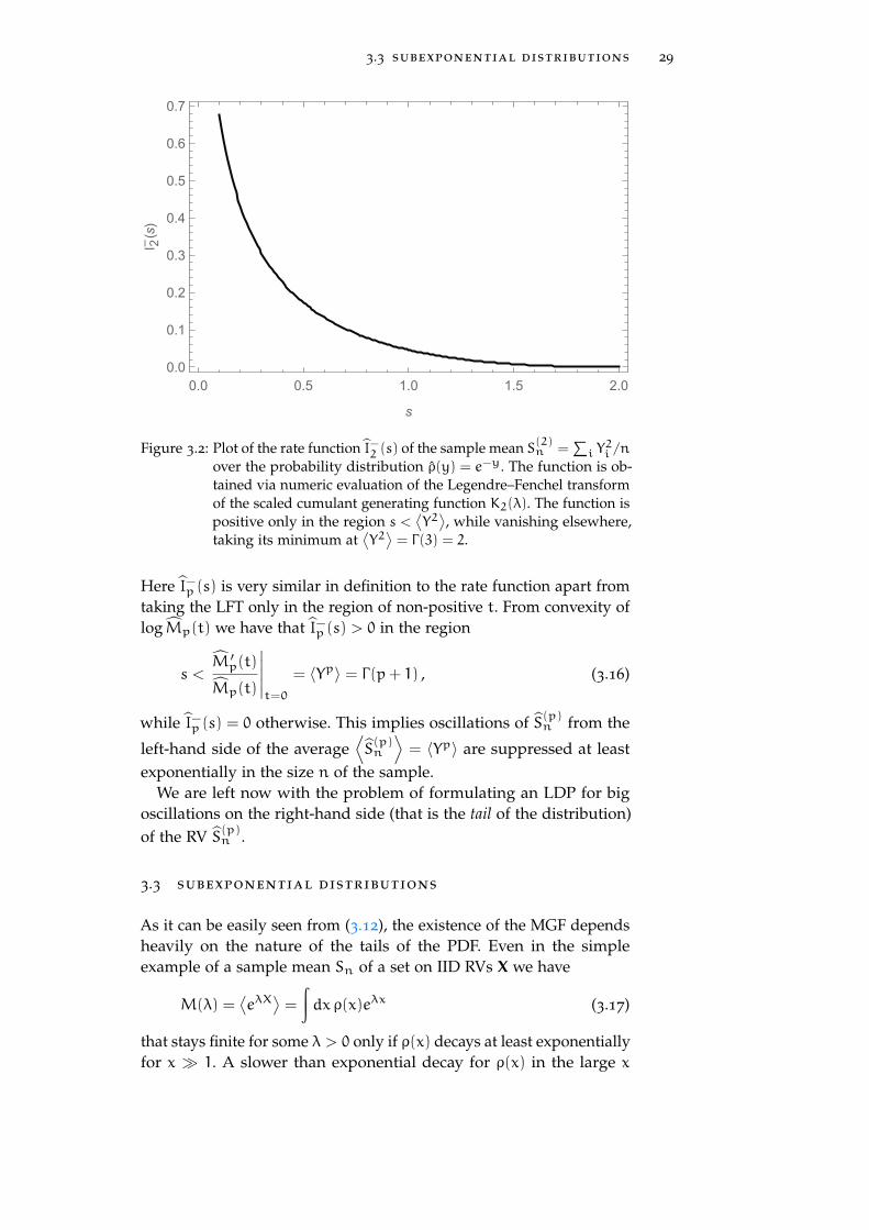
Here Î−p (s) is very similar in definition to the rate function apart fromtaking the LFT only in the region of non-positive t. From convexity oflogˆMp(t) we have that Î−p (s) > 0 in the region

s <ˆM ′

p(t)ˆMp(t)

t=0

= ⟨Yp⟩ = Γ(p+ 1) , (3.16)

while Î−p (s) = 0 otherwise. This implies oscillations of ˆS(p)n from the

left-hand side of the average⟨ˆS(p)n

⟩= ⟨Yp⟩ are suppressed at least

exponentially in the size n of the sample.We are left now with the problem of formulating an LDP for big

oscillations on the right-hand side (that is the tail of the distribution)of the RV ˆS(p)n .

3.3 subexponential distributions

As it can be easily seen from (3.12), the existence of the MGF dependsheavily on the nature of the tails of the PDF. Even in the simpleexample of a sample mean Sn of a set on IID RVs X we have

M(λ) =⟨eλX

⟩=

∫dx ρ(x)eλx (3.17)

that stays finite for some λ > 0 only if ρ(x) decays at least exponentiallyfor x ≫ 1. A slower than exponential decay for ρ(x) in the large x


limit prevents M(λ) to be defined on the positive real axis. Suchdistributions are known as subexponential or heavy-tailed distributions,provided that X > 0. They are defined by the limit

limx→∞

Fn(x)

nF1(nx)− 1

= 0 , n ∈ N. (3.18)

Let X∗n = maxi6n [X1, . . . ,Xn], then it can be easily seen that

limx→∞ Pr(X∗

n > x)

nF1(x)= 1, (3.19)

which allows for the interpretation that the large deviations of sumsof independent heavy-tailed random variables are typically realizedby just one of these variables taking a very large value. This is wellknown since the classical works of Heyde [17] and Nagaev [28, 29].As (3.20) suggests, we can explicit the asymptotic expression for largevalues of x

supx>dn

Fn(x)

nF1(nx)− 1

= o(1) , (3.20)

for a suitable sequence dn.Thus we are led to ask what kind of approximation to the tail

probabilities Fn(x) can be expected in the finite x region. A naturalbound comes from the CLT which implies, given ⟨X⟩ = µ,

⟨(X− µ)2

⟩=

σ2 < ∞,

supx

Fn(x) −Φ

(√n(x− µ)

σ

)= o(1) , (3.21)

where, once again, Φ denotes the standard error function. This isformally identical to the formulation we gave in Section 1.2. The lastrelation can be rewritten as

sup(x−µ)∈[an,bn]

Fn(x)

Φ(√

n(x−µ)σ

) − 1

= o(1), (3.22)

for

an =a√n

, bn =b√n

, a,b ∈ R . (3.23)

We can expect that an asymptotic expression of this type may holdeven for large deviations, namely that exists a sequence cn > bn,with cn

√n → ∞ sufficiently slowly and such that (3.22), with an =

O(n−1/2), holds. In his famous work, Cramér [7, 8] proved that,given the existence of the moment generating function of X in aneighborhood of the origin, (3.22) holds with an = O(n−1/2)andcn = o(n−1/3), while (3.22) fails in general for cn = O(n−1/3).

3.3 subexponential distributions 31

From the previous discussion it seems typical for Fn(x) (and itactually is, see [25]) that there exist two threshold sequences cn 6 dn

such that

Fn(x) ∼

⎧⎪⎨⎪⎩Φ(√

n(x−µ)σ

)x− µ ≪ cn

nF1(nx) x− µ ≫ dn

. (3.24)

The rigorous treatment of where these sequences arise from wouldrequire a number of technical tools; we refer to [25] for the details.Despite this, an heuristic argument can be provided: from the previousdiscussion it may have become clear that there exist different typesof large deviation results on different intervals, where either the CLTapplies or the extremes in the sample dominate Fn(x). A separatingsequence cn can be expected at the border, where both the CLT andthe extremal behavior overlap, i. e. where

Fn(x) ∼ Φ

(√n(x− µ)

σ

)∼ Pr(X∗

n > x) ∼ nF1(nx) . (3.25)

Thus a natural definition of bn comes from the relation

Φ(√

ncn)∼ nF1(ncn) ,

which implies

Φ(√

n(x− µ))= o

(nF1(nx)

), x ≫ cn .

On the other hand, the estimate of dn is rather more complicated.It can be retrieved both from extreme value theory arguments or moresimply by looking at the distribution of Sn −X∗

n/n, conditional uponSn = x, that is

Pr(Sn −

X∗n

n= u

Sn = x

)= n

pn−1(u)

pn(x)p1(nx−nu)

In this case the threshold sequence dn arise from pn−1(u), i. e. thequantity Sn −X∗

n/n, being asymptotically negligible. This implies thatthe large deviation of Sn occurs only on account of X∗

n.These heuristic arguments explain that the maximum of the sample

begins to have influence on the large deviations of Sn for x ≫ cn, andthat it dominates the large deviations when x ≫ dn. In the region(cn,dn), the partial sums and the extremes have influence. Therefore,in the latter region, explicit asymptotic expressions for Fn(x) are quitedifficult to obtain. The choice for the two threshold sequences heavilydepend on the nature of the tail of the distribution. A complete casestudy has been collected by Nagaev and Mikosh [25] where a numberof known results are presented.


3.3.1 Large deviations for sample mean of stretched exponential randomvariables

Let X be a set of n IID RVs distributed according to the exponentialdistribution ρ(x) as in (3.3) and S

(p)n (X) the sample mean of Xp

i as in(3.7).After a proper rescaling X

pi = Zi, this problem is formally identical to

the one of considering the sample mean SN(Z) of the set of IID RVs Z,sorted according to the probability density

ρ(p)(z) =z(1−p)/p

pe−z1/p z > 0 . (3.26)

Distributions of the type in (3.26) are called stretched exponentialdistributions due to a slower than exponential decay. This kind ofdistributions clearly exhibit a subexponential tail in the large z region.As a check we can evaluate

Pr(Z∗n > z) = 1− Pr(Z∗

n < z)

= 1− Pr(Z1 < z,Z2 < z, . . . ,Zn < z)

= 1−

n∏i=1

Pr(Zi < z)

which leads to

Pr(Z∗n > z) = 1−

[1− e−z1/p

]n. (3.27)

Thus, by replacing in (3.19), we have

limz→∞ Pr(Z∗

n > z)

nF1(z)= lim

z→∞1−

[1− e−z1/p

]nne−z1/p

= limz→∞ 1− e−ne−z1/p

ne−z1/p

= 1 .

As a consequence we can state the tail probability F(p)n (x) for the

sum Sn(Z) = S(p)n (X) takes the asymptotic form

F(p)n (x) ∼ Φ

(√n(x− µp)

σp

), x− µp ≪ c

(p)n

with µp, σp given in (3.10) and (3.11), while

F(p)n (x) ∼ nF

(p)1 (nx) = ne−(nx)1/p , x− µp ≫ d

(p)n .

This implies large deviations are less than exponentially dumped inthe size n of the sample.

3.4 the ldp for sum of powers of iid exponential rvs 33

It can be shown the threshold sequences are given by

c(p)n =

⎧⎨⎩c ·n− 13 p ∈ (1, 2)

c ·n1−p2p−1 p > 2

, (3.28)

d(p)n = d ·n

2−p2p−2 , (3.29)

for any c,d ∈ R+.As it can be easily seen, c(p)n always vanishes in the large n limit, beingc(p)n 6 O(n−1/3), due to the concentration of probability measure, that

is the CLT. On the other hand, the behavior of the threshold sequenced(p)n strongly depends on the parameter p that determines the behavior

of the heavy-tail. In fact, by taking the exponent in (3.29)

2− p

2p− 2> 0 ⇐⇒ p ∈ (1, 2) . (3.30)

Hence, provided that p ∈ (1, 2), the stretched exponential behaviorof F

(p)n (x) is recovered only for extremely large deviations, namely

(x− µp) ≫ nδ, δ > 0.As a check, as p → 1, that is as S(p)n approaches the sample mean Sn

of exponentially sorted random variables, d(p)n → ∞ and no stretched

exponential decay occurs. This is strongly related to the fact thatCramér’s condition still holds for distributions with proper exponen-tial decay like in (3.3). Thus the moment generating function is notill-defined and a rate function of the type in (3.5) can be recovered.

3.4 the large deviation principle for sum of powers of

independent exponential variables

Here we want to collect the results we found in the independent case.We started from the simple case of the sample mean Sn of IID RVssorted according to the exponential distribution ρ(x) = e−x. This casepresent no difficulties, for the MGF being finite up to a certain valueon the positive real axis, i. e. Cramér’s condition holds. By applyingCramér’s Theorem we found the moment generating function I(x) in(3.5) that assures large deviations from the mean value are suppressedexponentially in the number n of RVs in Sn.

We found the same procedure applies to the distribution ρm(x) in(3.8) (i. e. the marginal probability in the REMP) for the RV S

(p)n as

defined in (3.7), for finite values of m. Even in this case Cramér’s Theo-rem applies and the MGF Mp,m(λ) can be expressed as a power seriesof λ. Despite the fact that Im,p(x) has no simple analytic expression,it can be computed by numerically evaluating the LFT of the SCGF,as defined in (3.9), which leads for example to the RF in Figure 3.1.


As a result, once again we have an exponential decay in n for the tailprobability, that is

limn→∞ 1

nlog F

(p)n,m(s) = −Im,p(s) (3.31)

Since the parameter m in the distribution ρm(x) controls the numberof intervals in the REMP, that is the number of the RVs in the sumS(p)n , we took the limit for large m. By rescaling the RVs Y = 2mX we

found

limm→∞ ρm (y/(2m)) ≡ ρ(y) = e−y . (3.32)

Thus we focused on finding an asymptotic expression for the proba-bility F

(p)n (s) ≡ Pr

(ˆS(p)n (Y) > s)

, with the set of RVs Y sorted accord-ing to ρ(y), as in (3.3). This time we found that Cramér’s conditionis violated, that is the MGF ˆMp(λ) is defined only in the regionλ 6 0. Despite this, by using the Chernoff bound for the probabilityF(p)n (s) ≡ 1− F

(p)n (s), we had

limn→∞ 1

nF(p)n (s) 6 −Î−p (s) ,

where Î−p (s) is a regular positive function in the region s < ⟨Yp⟩ ≡µp = Γ(p+ 1), while it vanishes otherwise. In this case we have anLDP only on the left-hand side from the expected value of ˆS(p)n , wherethe probability of deviations exhibits an exponential dumping in n,while the right-hand side, that is for s > ⟨Yp⟩, has no proper bound.This suggests a different regime from the exponential one for theprobability F

(p)n (s) must be taken into account.

From the analysis made in Section 3.3 it should have become clearthat the problem of formulating an LDP for the RV ˆS(p)n (Y) is identicalto the one of finding the asymptotic expression for the probabilityPr(Sn(Z) > s), where the set of RVs Z is distributed according to thePDF ρ(p)(x) ∼ e−x1/p

as in (3.26). Here we found two threshold se-quences c

(p)n ,d(p)

n such that, for (s− µp) ≪ c(p)n the Gaussian regime

is still valid, even beyond the usual (s− µp) = O(n−1/2), that is thewell known CLT. Moreover, for (s− µp) ≫ dn, we observed the distri-bution of ˆS(p)n (Y) is influenced by the maximum of the RVs taking avery large value, that is the tail probability F

(p)n (s) ∼ nF

(p)1 (ns).

In conclusion we can state that, given a set of RVs Y distributedaccording to the exponential distribution

ρ(y) = e−y

an LDP holds for the RV ˆS(p)n (Y) with different bound in differentregions. In particular

F(p)n (s) 6 e−nÎ−p (s) , s− µp 6 0 , (3.33)

3.5 numerical simulations 35

with I−p (s) as given in (3.15), while

F(p)n (s) ∼

⎧⎪⎨⎪⎩Φ(√

n(s−µp)σp

)0 < s− µp ≪ c

(p)n

ne−(ns)1/p s− µp ≫ d(p)n

, (3.34)

with µp, σp given in (3.10) and (3.11), and with the threshold se-quences c

(p)n ,d(p)

n as given in (3.28) and (3.29).Thus the distribution of ˆS(p)n (Y) exhibits a different scaling with n

on the left and on the right-hand side of the average value µp. In par-ticular, while in the region s ≪ c

(p)n deviations are always suppressed

exponentially in n, we have for s ≫ d(p)n that the probability assumes

a stretched exponential behavior, with scaling speed n1/p, makingextreme values more likely.

3.5 numerical simulations

In this section we want to discuss the numerical methods to havean estimate of the shape of the rate function. This problem is quitedifficult to approach, mainly because of the nature of large deviations.From the previous discussion it should have become clear that LDThas to deal with extreme value theory and the probability of rareevents, while the number of RVs is very large. Since from CLT wehave that probability concentrates around the typical values of thedistribution as the number of RVs increases, sampling rare events,that is extracting a precise asymptotic trend for the tail probability,can result in an unfeasible task. In other words, given the samplemean Sn of RVs, regardless the speed of the scaling, large deviationprobabilities are always exponentially suppressed in n, while, to obtainan accurate approximation for the rate function I(s), we would need n

to be large. This comes from the asymptotic expression of the PDF forlarge values of n retaining only the dominant term in the exponential,while neglecting subleading orders.

There are different techniques to treat this problem: here we refer toone of the most simple tools we can imagine to extract a rate functionfrom numerical simulations, that is the direct sampling.

3.5.1 Direct sampling method

The problem addressed here is to obtain a numerical estimate ofthe PDF pSn

(s) for the real RV Sn satisfying an LDP, and to extractfrom this an estimate of the rate function I(s). To be general, we willconsider Sn = Sn(X) to be a function of the set X of n RVs, which, atthis point, are not necessarily IID.

Numerically, we cannot of course obtain pSn(s) or, equivalently, I(s)

for all s ∈ R, but only for a finite number of values s, which we take


for simplicity to be equally spaced with a small step ∆s. Thus, we canestimate the coarse-grained PDF

pSn(s) =

Pr (Sn ∈ [s, s+∆s])

∆s=

Pr(Sn ∈ ∆s)

∆s, (3.35)

where ∆s ≡ [s, s+∆s] denotes the interval of amplitude ∆ anchoredto the value s.

To construct this estimate, we follow the statistical sampling or MonteCarlo method, which we can broke down into the following steps

• generate the sample X(j)Lj=1 of L copies of the sequence X fromits PDF;

• obtain from this sample, the set s(j)Lj=1 of the realizations ofSn, that is

s(j) = Sn(X(j)) ;

• estimate the probability Pr(Sn ∈ ∆s) by evaluating the samplemean

PL(∆s) ≡1

L

L∑j=1

χ∆s

(s(j))

,

where χA(x) denotes the indicator function of the set A, that is

χA(x) ≡

⎧⎨⎩1 x ∈ A

0 x ∈ A;

• use the sample mean PL(∆s) to estimate the probability distribu-tion of Sn:

pL(s) ≡PL(∆s)

∆s=

1

∆sL

L∑j=1

χ∆s

(s(j))

.

Note that pL(s) above is nothing but an empirical vector for Snor, equivalently, a histogram normalized over the total counts of thesample s(j)Lj=1. The reason for choosing pL(s) as our estimator ofpSn

(s) is that it is an unbiased estimator, in the sense that

⟨pL(s)⟩ = pSn(s)

for any L. Moreover, we know from the LLN that pL(s) converges inprobability to its mean pSn

(s) as L increases. Therefore, the larger oursample, the closer we should get to a valid estimation of pSn

(s).The rate function can be easily computed by recalling the symptotic

expression of the PDF, that leads to

I(L)n (s) =

1

nlogpL(s) . (3.36)


We can repeat the whole process for larger and larger integer valuesof n and L to improve the accuracy of the rate function.

This method presents a severe limitation: a basic rule in statisticalsampling, suggested by the LLN, is that an event with probability P

will appear in a sample of size L roughly LP times. Thus to get at leastone instance of that event in the sample, we must have L > P−1, asan approximate lower bound for the size of our sample. In terms ofLDT we see that if a RV Sn satisfies an LDP with rate function I(s)

and speed n then we would need L > enI(s) to see just one event. Asa consequence, increasing the size n of the sample mean to maximizeaccuracy, determines the number of instances L to get exponentiallylarge.

3.5.2 Simulation results

Here we collect the results of the numerical computations in theindependent case. The simulations presented here are obtained viathe direct sampling method discussed in the previous paragraph. Asa consequence of the limitations of this procedure, the plots shouldbe considered as a qualitative check, without claiming to confirm norreject the rigorous results obtained in Section 3.4.

As a first check, we extrapolated the rate function I−p (s) for the RV

S(p)n we found in (3.15) from the direct sampling of the exponential

distribution. As an example, in Figure 3.3 the plot of the rate functionI−2 (s) is shown in gray with the estimated rate functions, as in (3.36),for fixed L = 107 instances of the sample mean S

(2)n and for different

values of n. As we can see, the larger the value of n the closer the pointsare to the expected rate function. On the other hand, it is important tonotice that the range of the simulations, that is the interval on whichthe estimated rate function is defined, decreases as the number of RVsn accounted for in S

(2)n becomes larger. This directly follows from the

deterioration of the statistics far away from the expected value dueto the direct sampling method: in fact, as n increases we are probingonly the (small) Gaussian deviations, that is the CLT.

Moreover, we can check the exponential scaling of the tail probabilityF(p)n (s) is n1/p, as we found in (3.34). An estimation of F

(p)n (s) =

Pr(S(2)n > s

)can be obtained in the same fashion of the previous

paragraph, by counting the number of instances having a realizations(j) > s and normalizing over the total number of instances L.By recalling that

F(p)n (s) ∼ e−n1/p(x−µp)

1/p

,

we can extract the exponent of n from the relation

log[− log F

(p)n (s)

]≡ logQ

(p)n (s) =

1

plogn+ log(x− µp)

1/p . (3.37)


Thus, from a linear regression in logn, we can obtain the exponentas the slope of the fitting line. An example is shown in Figure 3.4for the case p = 5, which we expect to show a more pronouncedsubexponential tail, with L = 107 number of instances and differentvalues of logn.


n=10

n=30

n=50

n=100

0.0 0.5 1.0 1.5 2.00.0

0.1

0.2

0.3

0.4

0.5

0.6

0.7

s

I 2–(s)

Figure 3.3: Plot of the rate function ˆI−2 (s) as in (3.15) of the sample mean

S(2)n =

∑i Y

2i /n over the exponential PDF ρ(y) = e−y and the

estimated rate functions from direct sampling method for differentvalues of n. As the number of RVs n increases the estimatedrate functions (i. e. the PDF of Sn) get closer to the asymptoticexpression ˆI−2 (s), while the range of definition shrinks due toconcentration of measure, that is the central limit theorem.

0.20002 log(n) +1.44484

3 4 5 6 7

2.0

2.2

2.4

2.6

2.8

log(n)

logQp

Figure 3.4: Linear regression as defined in (3.37) to check the scaling speed

for the tail probability F(5)n = Pr

(S(5)n > s

)in the subexpo-

nential region (p = 5). The slope of the fitting line coincide

with the exponent of n in the asymptotic expression of F(5)n ∼

exp−n1/5(x− Γ(6))1/5 as in (3.34). The result matches with theexpected value p−1 = 5−1 = 0.2.

4A L A R G E D E V I AT I O N P R I N C I P L E F O R T H EAV E R A G E C O S T O F O N E D I M E N S I O N A L R E M P

In this section we collect the main results we obtained for the distri-bution of the average cost of the one dimensional matching problemdiscussed in Chapter 2 in the large n limit. We start by proving thetotal cost in REMP is asymptotically normally distributed, that is theprobability measure concentrates around the typical value, as stated bythe central limit theorem. We show that actually the Gaussian regimecan be extended to moderate large deviations, for a suitable thresholdsequence c

(p)n as in the case of independent identically distributed

random variables. A short comment on numerical simulations is pro-vided at the end of this chapter, where some interesting features ofthe distribution can be noticed.

4.1 the central limit theorem for dependent variables

In the following we want to explicit that the limiting distribution forn → ∞ of the total optimal cost E(µ∗) for the REMP, as gven in (2.6),is Gaussian. Although this is not a result of LDT, we want to stressthat the CLT does not apply in its standard formulation to dependentvariables, as the one we are considering in our problem. Here werefer to the work of Darling [9] which proved this limit holds for thegeneralized sum

W(h)n =

2n∑i=0

h(ϕi) (4.1)

for a wide range of real-valued functions h.

4.1.1 The fundamental formula

Let us start by noting that, given ϕ = (ϕ0, . . . ,ϕ2n) the set of subin-tervals in which the unit interval Λ = [0, 1] is divided by 2n randompoints, for f = (f0, . . . , f2n) a set of real-valued function, it holds⟨

2n∏j=0

fj(ϕj)

⟩=

(2n)!2πi

∫c+i∞c−i∞ dz ez

⎡⎣ 2n∏j=0

∫∞0

drj e−rjzfj(rj)

⎤⎦ . (4.2)

Here c is a constant larger than all the abscissas of convergence of thecorresponding Laplace transforms of the fi, the path of integrationbeing on the complex plane Re(z) = c. The formula in (4.2) can be

41

42 an ldp for the average cost of remp

obtained by observing that the expectation value of the product offi(ϕi) = fi(xi+1 − xi), 0 = x0 6 x1 6 x2 · · · 6 x2n 6 x2n+1 = 1, isgiven by⟨

2n∏j=0

fj(ϕj)

⟩=(2n)!

∫10

dx2n

∫x2n

0

dx2n−1

· · ·∫x2

0

dx1 f0(x1)f1(x2 − x1) . . . f2n(1− x2n) .

This is simply the convolution f0 ∗ f1 ∗ · · · ∗ f2n(1), where

g ∗ h(x) ≡∫x0

dt g(x− t)h(t) .

Hence, by recalling that the Laplace transforms multiply under convo-lution, we obtain∫∞

0

dx f0 ∗ f1 ∗ · · · ∗ f2n(x)e−zx =

2n∏j=0

∫∞0

drj fj(rj)e−zrj .

Now, by applying the complex inversion for the Laplace transformand setting x = 1, we obtain (4.2).

The formula we just found is completely general and allows toevaluate numerous expectation values over the probability distributionof uniform spacings. By simply setting fi(ϕi) = eiξh(ϕi) we have

⟨eiξW

(h)n

⟩≡

⟨2n∏i=0

eiξh(ϕi)

⟩

=(2n)!2πi

∫c+i∞c−i∞ dW eW

[∫∞0

dr e−rW+iξh(r)

]2n+1

,

(4.3)

that is the characteristic function, i. e. the Fourier transform of thedistribution, for the generalized sum W

(h)n .

4.1.2 The Gaussian regime

The proof of asymptotic normality of the distribution of the total costin REMP follows directly from the evaluation of the characteristicfunction. It is useful to recall that in the REMP we have a set of(2n + 1) RVs, namely the subintervals ϕ, while the total optimalcost E(p)

n = nε(p)n is evaluated by summing only on the set ϕodd =

(ϕ1, . . . ,ϕ2n−1). Thus, from (4.3) we have

F(p)n (ξ) ≡

⟨eiξE

(p)n

⟩=

(2n)!2πi

∫c+i∞c−i∞ dE eE

[∫∞0

dr e−rE+iξrp]n [∫∞

0

dr e−rE

]n+1

.

(4.4)

4.1 the central limit theorem for dependent variables 43

Now, letting

ξ = (2n+ 1)p−1/2t , E = (2n+ 1)z ,

and shifting the contour parallel to itself we have

F(p)n

((2n+ 1)p−1/2t

)=

(2n+ 1)!(2n+ 1)2n+1

1

2πi

∫c+i∞c−i∞ dz

e(2n+1)z

z2n+1[Bn(z, t)]n , (4.5)

where

Bn(z, t) ≡ (2n+ 1)z

∫∞0

dr e−r(2n+1)z+it(2n+1)p−1/2rp . (4.6)

As it will turn out, [Bn(z, t)]n is actually a bounded function witha well defined limit for n → ∞ for t bounded and ∀z. Thus theintegral in (4.5) can be evaluated by just taking the dominant termof e(2n+1)zz−(2n+1) = e(2n+1)f(z) by a saddle point approximation,with f(z) = z− log z. Now, solving for f ′(z) = 0, we have z = 1, whilef ′′(1) = 1. Hence in (4.5) we simply take c = 1 to get the contour ofsteepest descent. By setting

z = 1+iy√

2n+ 1(4.7)

with

y ∈ In =[−(2n+ 1)δ, (2n+ 1)δ

]δ ∈

(0,

1

2

), (4.8)

the integral has its essential contribution in this range. It is usefulto stress out the Gaussian regime results as a consequence of thisapproximation, for the CLT being valid in an interval around theaverage value of order

√n. Plugging the expression of z = z(y) as in

(4.7) in (4.5) we have for the constants preceding the integral

(2n+ 1)! e2n+1

(2n+ 1)2n+ 32

1

2π=

1√2π

+ o(1)

which follows from Stirling’s approximation of the factorial (2n+1)! =Γ(2n+ 2). Thus, for the characteristic function in (4.5), we have

F(p)n

((2n+ 1)p−1/2t

)=

∫In

dy√2π

e−y2/2 [Bn(z, t)]n [1+ o(1)] ,

(4.9)

Now we take the asymptotic expansion in (4.6) that gives

Bn(z, t) = (2n+ 1)z

∫∞0

dr e−r(2n+1)z

×(1+ it(2n+ 1)p−1/2rp +

(it)2

2(2n+ 1)2p−1r2p + . . .

)= 1+ (it)

Γ(p+ 1)

zp√2n+ 1

+(it)2

2

Γ(2p+ 1)

z2p(2n+ 1)+ o(n−1) ,


and letting z = z(y) we get

n logBn(z, t) = n log[1+ (it)

Γ(p+ 1)

zp√2n+ 1

+(it)2

2

Γ(2p+ 1)

z2p(2n+ 1)+ o(n−1)

]= (it)

Γ(p+ 1)√2

√n+ ty

pΓ(p+ 1)

2

+(it)2

2

Γ(2p+ 1) − Γ(p+ 1)2

2+ o(1) .

Plugging this estimate in (4.9) we obtain

F(p)n

((2n+ 1)p−1/2t

)e−it

Γ(p+1)√2

√n

= e−t2

2Γ(2p+1)−Γ(p+1)2

2

∫In

dy√2π

e−y2/2+ytpΓ(p+1)/2 (1+ o(1)) ,

and by taking the limit of large n we get

limn→∞

⟨exp

it

((2n+ 1)p−

12E

(p)n −

Γ(p+ 1)√2

√n

)⟩= lim

n→∞⟨

expit(2n)p−1/2

[E(p)n −

Γ(p+ 1)

2pnp−1

]⟩= exp

−t2

2

2Γ(2p+ 1) − 2Γ(p+ 1)2

4

×∫∞−∞

dy√2π

e−y2/2+ytpΓ(p+1)/2

= exp−t2

2

2Γ(2p+ 1) − (2+ p2)Γ(p+ 1)2

4

.

Since the Fourier transform of a normal distribution is normal dis-tributed in the conjugate variable, we have established the assumption.As a consequence, we have also an independent derivation for theasymptotic moments given in (2.19) and (2.22).

4.2 the extension to large deviations

Here we collect the results of large deviations which we obtained forthe average cost for the REMP. The main achievement is the extensionof Gaussian regime we just extracted to a broader interval.

4.2.1 The Gaussian moderate deviations

In this section we will try to show the asymptotic normality of thedistribution of the average cost in the REMP can be extended in alarger region than the typical one of CLT. As in the previous chapter,to properly formulate an LDP for the average cost we would need anumber of technical tools of probability theory. In here we refer to thework of Mirakhmedov [26, 27], that found a number of precise large

4.2 the extension to large deviations 45

deviations for the generalized sum Wn, as in (4.1), under suitableconditions of the function h.

The topic seems to be of great interest for asymptotic efficiency ofgoodness-of-fit tests [15, 33]. These are aimed to confirm or reject thehypothesis that a certain data set is distributed according to some apriori PDF, which in this case is the uniform distribution on the unitinterval Λ. Typically, this is achieved by looking at the discrepancybetween the expected and empirical value of a generalized sum W

(h)n ,

for some suitable function h of the spacings between successive points.Although a number of possible choices is given for the actual functionh, it seems common to choose h(x) = x2, called Greenwood statistics,named after Major Greenwood [16] who firstly introduced this test toestimate the distribution of genes in the chromosomes of living organ-isms. The asymptotic expression of the tail probability for this kind ofstatistics has a specialized result, as it will be shown subsequently.

After the discussion in Chapter 3, it should have become clear thatthe right observable to be taken into account to formulate an LDP isthe rescaled RV φ = 2nϕ, which has a well defined distribution inthe large n limit. In particular, we will refer to the average cost peredge of the REMP, namely to the quantity ε

(p)n = (2n)pε

(p)n whose

limit moments, given in (3.10) and (3.11), are positive and finite.As in Section 3.3, the validity of asymptotic normality for the dis-

tribution of the RV ε(p)n is constrained by a threshold sequence c

(p)n .

This defines the region where the approximation holds, namely howfar from the expected value

⟨ε(p)n

⟩the deviation can get for the dis-

tribution to be Gaussian. In this case the sequence arises from notingthat the problem of finding the distribution of the random vectorφ = (φ0, . . . ,φ2n) can be mapped in the one of 2n+ 1 exponentialRVs Z = (Z0, . . . ,Z2n) conditional to their sum being 2n+ 1. Moreexplicitly, by denoting with D(X) the distribution of the random vectorX, we have

D (φ) = D(Z|S2n+1(Z) = 1) , (4.10)

where, as always, Sn(X) stands for the sample mean of the random vec-tor X. In this case it can be proved that, for any p > 1, the asymptoticexpression for the tail probability takes the form

Pr(ε(p)n > x

)∼ Φ

⎛⎜⎝ n

var[ε(p)n

](x− µp)

⎞⎟⎠ , 0 < x−µp ≪ c(p)n ,

(4.11)

where

c(p)n = cn = c ·

√logn

n, c ∈ R+ , (4.12)


while µp = ⟨Zp⟩ as given in (3.10) and var[ε(p)n

]as in (2.22). It is

important to notice that the expectation value of ε(p)n is exactly µp

only in the large n limit, namely

limn→∞

⟨ε(p)n

⟩= µp .

This fact arises exactly from (4.10), the difference of the two distribu-tion being o(1) in the region defined by (4.12).

This result can be specialized to the case p = 2, that is the Green-wood statistics: in his work Mirakhmedov shows that the cumulants ofthe RV ε

(2)n and the ones of S(2)n (Z) can be both bounded by the same

quantity, making the two RVs asymptotically equivalent. This methodof extracting large deviation probabilities is known as Statulevicious’condition [2], which allows to verify that ε(2)n is normally distributedin a region broader than the one defined by (4.12). This results for thetail probability taking the limit expression

Pr(ε(2)n > x

)∼ Φ

(√n(x− µ2)

σ2

), 0 < x− µ ≪ c

(2)n , (4.13)

with

c(2)n = c ·n−1/3 , c ∈ R+. (4.14)

As a consequence, from both (4.11) and (4.13), we can state theprobability distribution is exponentially suppressed in the size of thesample with speed n due to ε

(p)n being normally distributed up to a

distance from the average value defined by the threshold sequencesgiven in (4.12) and (4.14).

4.2.2 Large deviations for the tail probability

In the previous section we discussed the extension of the Gaussianregime up to a threshold sequence c

(p)n . As in the independent case

discussed in Section 3.4, we tried to establish an LDP even in thelarge x region, where we suspect the behavior of the tail probabilityPr(ε(p)n > x

)is qualitatively identical to the one of the independent

case. As already mentioned, this was driven by the observation that,as the number of spacings n increases, the spacings ϕ (that is φ) actmore and more like independent and identically distributed. Thiscomes from the RVs being weakly dependent, as we already pointedout in Section 2.3.1. As a matter of fact, no rigorous result couldbe provided to support this assumption. Nevertheless, a number ofnumerical simulations were carried out to see if any LDP could beextracted from the directly inspecting the distribution of costs.


4.3 numerical simulations

In this section we present the results of the simulations carried outwith the direct sampling method discussed in Section 3.5.1.Firstly, we checked that the average cost per edge ε

(p)n is normally

distributed for large values of n. An example of this fact is illustratedin Figure 4.1 for the p = 2 case, where the normalized histogramof the average cost pL(x), sampled over L = 107 instances, and theexpected Gaussian distribution is given. Actually, the convergence tothe normal distribution comes quite rapidly as n increases: the heavytail behavior for n = 50, which is stressed out in the logarithmic plot(Figure 4.1b), gets almost entirely suppressed as n = 500 (Figure 4.1d),where no appreciable subexponential trend can be noticed.

It is useful to recall from Section 3.3.1 that, in case of independentRVs, the value p = 2 was quite exceptional. For smaller values, thatis for p ∈ (1, 2), the subexponential tail can be recovered only in theregion of x ≫ nδ, with δ > 0, that is for extremely large deviationsfrom the expected value. On the other hand, for p > 2, the stretchedexponential tail dominates a region that gets closer and closer to theexpected value µp as n increases.

Driven by this observations we could ask if a similar behaviorapplies to the (correlated) case of REMP. Namely, we could ask if, evenfor large values of n, a stretched exponential tail can be observed forp > 2. In Figure 4.2 we collected the distribution of the average costin the case p = 5 for different values of n with the expected Gaussiandistribution as a comparison. It appears clearly that the convergenceto the Gaussian regime is slower than the previous case as n increases,mostly due to the variance being larger as a consequence of larger p.Nevertheless, especially in the logarithmic plot (see Figure 4.2b), itappears the distribution exhibit a subexponential tail in the region oflarge x, even for values of n where the Gaussian regime is dominant(Figure 4.2f). This could suggests a slower than exponential dumpingin n may occur in the large x region, as in the case of independentRVs. Although, given the great inefficiency of the sampling methodwe used for large deviations, extracting a precise speed of scaling forthe tail distribution of the average cost is unfeasible. This, as alreadydiscussed in Section 3.5.1, has to deal with both the nature of rareevents and the limitations of this procedure. As a consequence, noproper bound for the tail probability far away from the expected valuecan be extracted from the numerical simulations.

4.4 conclusion and outcomes

As already pointed out, we have proved the distribution of the averagecost in the REMP is normally distributed around the typical value inthe limit of large n, that is the Gaussian regime applies in a region


predicted by the CLT. We provided some motivations to the fact thatthis regime can be extended in a broader region than the classical oneby using results coming from statistical inference and goodness-of-fittests.

We would have liked to obtain some rigorous results regarding thebehavior of the tail probability of the distribution of cost in the verylarge x region. This would have allowed to establish a proper largedeviation principle for the whole distribution of the average cost. Asa consequence, the characterization of probability of rare events andhow fast values different from the typical one become unlikely is notcompletely resolved. This is a challenging task to accomplish, mostlybecause of non-trivial correlations induced by the Euclidean distance.Numerical simulations that we performed, despite their limitations,seems to suggest that the independent and the correlated case couldhave a similar asymptotic expression far away from the expectedaverage cost.

Actually, this remains an open problem that needs to be furtherinvestigated.

4.4 conclusion and outcomes 49

0.5 1.0 1.5 2.0 2.5 3.0 3.50.0

0.2

0.4

0.6

0.8

1.0

x

p(x)

p=2, n=50

μ=1.941, σ=0.467

(a)

1 2 3 4 5 6 7

10-5

10-4

0.001

0.010

0.100

1

10

xlog(p(x))

p=2, n=50

μ=1.941, σ=0.467

(b)

0.5 1.0 1.5 2.0 2.5 3.0 3.50.0

0.5

1.0

1.5

2.0

2.5

3.0

x

p(x)

p=2, n=500

μ=1.994, σ=0.154

(c)

1 2 3 4 5 6 7

10-5

10-4

0.001

0.010

0.100

1

10

x

log(p(x))

p=2, n=500

μ=1.994, σ=0.154

(d)

Figure 4.1: Normalized histogram of the average cost ε(2)n for p = 2, fromthe direct sampling method. The number of instances L = 107 isfixed and different values of n are collected ( n = 50 in (a) and(b), n = 500 in (c) and (d)). Convergence towards the expectednormal distribution (in black, with given mean and variance)is quite fast as n increases: while the probability concentratesaround the typical value from (a) to (c), the subexponential tailwhich can be observed in the logarithmic plot (b) for n = 50 isalmost entirely suppressed in (d) for n = 500.


50 100 150 200 250 3000.000

0.002

0.004

0.006

0.008

0.010

0.012

x

p(x)

p=5, n=500

μ=118.080, σ=79.697

(a)

0 500 1000 1500 2000 2500 3000

10-7

10-5

0.001

0.100

x

log(p(x))

p=5, n=500

μ=118.080, σ=79.697

(b)

100 150 200 250 3000.000

0.005

0.010

0.015

0.020

0.025

0.030

x

p(x)

p=5, n=104

μ=119.909, σ=18.466

(c)

100 200 300 400 500

10-7

10-6

10-5

10-4

0.001

0.010

0.100

x

log(p(x))

p=5, n=104

μ=119.909, σ=18.466

(d)

100 150 200 250 3000.00

0.01

0.02

0.03

0.04

0.05

0.06

0.07

x

p(x)

p=5, n=105

μ=119.998, σ=5.849

(e)

100 150 200 250

10-7

10-6

10-5

10-4

0.001

0.010

0.100

x

log(p(x))

p=5, n=105

μ=119.998, σ=5.849

(f)

Figure 4.2: Normalized histogram of the average cost ε(5)n for p = 5, fromthe direct sampling method. The number of instances L = 107 isfixed and different values of n are collected. Convergence towardsthe expected normal distribution (in black, with given mean andvariance) happens to be slower in n than the p = 2 case (see Fig-ure 4.1), although the Gaussian regime is almost totally recoveredin (e) for n = 105. While the probability concentrates around thetypical value from (a) to (e), the subexponential tail in the loga-rithmic plot (b) for n = 500 persists even for larger values of n,as in (f) for n = 105. This may suggest the subexponential regimefor large values of x can reflect in a subexponential dumping in n

of the tail probability.

Part II

A P P E N D I X

AT H E L E G E N D R E - F E N C H E L T R A N S F O R M

In this appendix we want to give a proper definition and enunciatesome useful properties of the Legendre-Fenchel transform, which areextensively used during the dissertation.

a.1 definition and first properties

Let f : R → R be a real-valued function: we define the Legendre-Fenchel transform (LFT) of f(x) by the variational formula

f∗(k) ≡ supx∈R

[kx− f(x)] . (A.1)

In the same way, the LFT of f∗(k) can be defined as

f∗∗(x) ≡ (f∗(k))∗ = supk∈R

[kx− f∗(k)] , (A.2)

which corresponds also to the double LFT of f(x). It is important tonotice LFT is not necessarily involutive: that is to say, f∗∗ does not neednecessarily to be equal to f.

Obviously, the LFT can be defined using an infimum rather than asupremum:

g∗(k) = infx∈R

[kx− g(x)] . (A.3)

This can be shown to be equivalent to expression in (A.1) by introduc-ing minus signs at the right place. Explicitly

−f∗(k) = − supx∈R

[kx− f(x)]

= infx∈R

[−kx+ f(x)]

so that, by setting g(x) = −f(x), we have g∗(k) = −f∗(−k). That is,defining the LFT by the infimum as in (A.3) simply results in the pointreflection of the function f∗.

The LFT is often referred to in physics as Legendre transform. Actuallythe Legendre transform is simply defined by considering

f∗(k) = kxk − f(xk) (A.4)

where xk is determined as the solution of the equation

d

dxf(x) ≡ f ′(x) = k . (A.5)

53

54 the legendre-fenchel transform

This form is more limited in scope than the LFT since it applies only todifferentiable and convex functions, as we will see later. In this sense,the LFT is a generalization of the Legendre transform, which extendsto nonconvex, non differetiable functions.

The definition of the LFT given in (A.1) can trivially be generalizedto functions defined on higher-dimensional spaces, namely functionsf(x) : Rd → R, with d a positive integer, by replacing the normalreal-number product kx by the scalar product k · x, where k and x areboth d-dimensional vectors.

a.2 theory of legendre-fenchel transform

The theory of LFT deals almost entirely with two question

• how the choice of the function f affects the expression of f∗;

• when an LFT is involutive, i. e. when it holds f∗∗ = f.

These two questions are answered by using a fundamental conceptof convex analysis known as a supporting line. We say that the func-tion f : R → R admits a supporting line at x ∈ R if there exists a realconstant α such that

f(y) > f(x) +α(y− x) , ∀y ∈ R . (A.6)

The constant α is called the slope of the supporting line. We furthersay that a supporting line is strictly supporting at x if

f(y) > f(x) +α(y− x) , ∀y = x . (A.7)

From now on we will replace the expression ”f admits a supportingline in x” with the one ”f is convex in x”. If, on the other hand, fdoes not admit a supporting line, we will say f is nonconvex at x. Itshould be clear that, for any differentiable function f, the property ofadmitting a supporting line in x, i. e. to be convex at x, simply impliesf ′′(x) to be positive, while α = f ′(x).

Ideed, it can be shown that the LFT f∗(k) of a real-valued functionf(x) is always convex for any k ∈ R. This requires the double transformf∗∗(x) to be a convex function as well, without being guaranteed f(x)

was convex in the first place. We now understand why the equalityf∗∗(x) = f(x) does not always hold, namely if f is nonconvex in x thenwe are guaranteed that f∗∗(x) = f(x).

We can now answer to the first question by using the result of thefollowing theorem.

Theorem A.2.1 If f admits a supporting line at x with slope k, then theLFT f∗ admits a supporting line at k with slope x.

This fact specializes to the case of f being a strictly convex function.

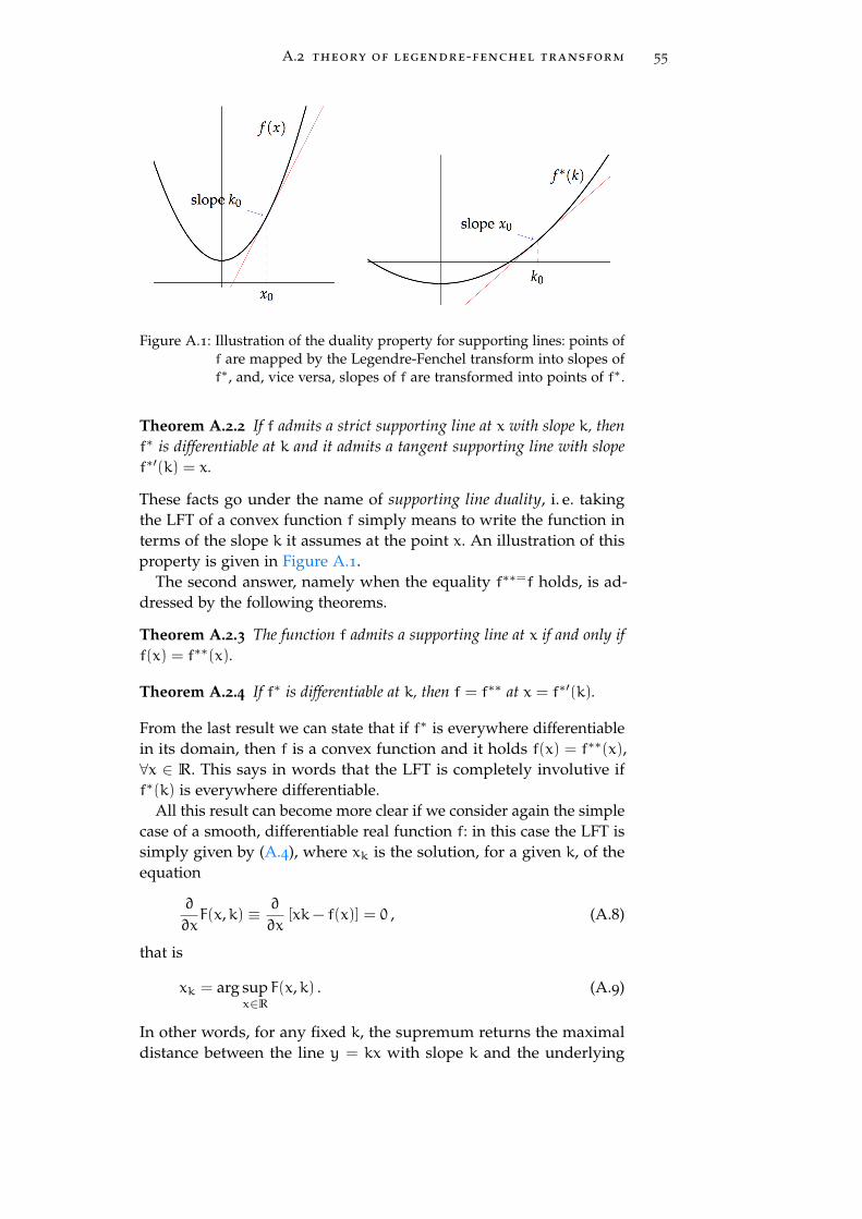
A.2 theory of legendre-fenchel transform 55

Figure A.1: Illustration of the duality property for supporting lines: points off are mapped by the Legendre-Fenchel transform into slopes off∗, and, vice versa, slopes of f are transformed into points of f∗.

Theorem A.2.2 If f admits a strict supporting line at x with slope k, thenf∗ is differentiable at k and it admits a tangent supporting line with slopef∗′(k) = x.

These facts go under the name of supporting line duality, i. e. takingthe LFT of a convex function f simply means to write the function interms of the slope k it assumes at the point x. An illustration of thisproperty is given in Figure A.1.

The second answer, namely when the equality f∗∗=f holds, is ad-dressed by the following theorems.

Theorem A.2.3 The function f admits a supporting line at x if and only iff(x) = f∗∗(x).

Theorem A.2.4 If f∗ is differentiable at k, then f = f∗∗ at x = f∗′(k).

From the last result we can state that if f∗ is everywhere differentiablein its domain, then f is a convex function and it holds f(x) = f∗∗(x),∀x ∈ R. This says in words that the LFT is completely involutive iff∗(k) is everywhere differentiable.

All this result can become more clear if we consider again the simplecase of a smooth, differentiable real function f: in this case the LFT issimply given by (A.4), where xk is the solution, for a given k, of theequation

∂

∂xF(x,k) ≡ ∂

∂x[xk− f(x)] = 0 , (A.8)

that is

xk = arg supx∈R

F(x,k) . (A.9)

In other words, for any fixed k, the supremum returns the maximaldistance between the line y = kx with slope k and the underlying

56 the legendre-fenchel transform

x

yf(x)

y = kx

xk

Figure A.2: Geometrical representation of the Legendre transform: maximiz-ing the function F(x,k) = kx− f(x) with respect to x is equivalentto finding the maximal distance between the line y = kx and theunderlying function f(x). Here the maximal distance (red) havinglength kxk − f(xk), where xk is determined by the differentialequation ∂xF(x,k) = 0.

function y = f(x). A geometrical interpretation of this fact is given inFigure A.2. Obviously there could be more than one critical pointsof F(x, k) that would solve the differential equation in (A.8). To makesure that there is actually only one solution for every k ∈ R, weneed to require f ′ to be monotonically increasing in the variable x,while f ′(x) → ±∞ for x → ±∞. With these two assumptions we areguaranteed that there exists a unique value xk that satisfies

f ′(xk) = k ,

and which maximizes F(x,k). Thus we have proved the LFT reducesto a simple Legendre transform for the case of differentaible andstrictly convex functions, the latter descending from monotonicity off ′. As a consequence of this fact, from Theorem A.2.3 we also havef∗∗(x) = f(x), ∀x ∈ R, meaning the LFT is completely involutive. Thus,from the definition we gave in (A.2) we have

f∗∗(x) = f(x) = xkx − f∗(kx) , (A.10)

where, analogously to (A.9), kx is the unique solution of the equation

f∗′(k) = x . (A.11)

Now we could ask what would happen if we remove the assumptionthat f ′(x) is monotone, that is if f is a differetiable nonconvex functionof x. In this case we have at least one open interval I = (x1, x2) inwhich the function f does not admit a supporting line. This means,by recalling the results in Theorem A.2.1 and Theorem A.2.2, that thepoints in the interval I have no representation in terms of the LFT f∗.In other words, there is no point k of f∗ which admits a supportingline with slope in the range (x1, x2).

A.2 theory of legendre-fenchel transform 57

Figure A.3: On the right a nonconvex smooth function f(x). The doubleLegendre-Fenchel transform f∗∗(x) coincides with the convexenvelope of f(x): it is obtained by replacing the nonconvex branchof f with the supporting line connecting the two convex branches.

From the definition we gave in (A.6), it is easy to see that the pointsx1 and x2 must share the same supporting line. Namely, since f isdifferentiable, the supporting line of f in x1 coincides with its tangentline

y = f(x1) + f ′(x1)(x− x1) 6 f(x) , ∀x ∈ R ,

and taking x = x2 it follows that f ′(x2) = f ′(x1). As a consequenceThe LFT f∗ must have a non differentiable point at kc, with kc =

f ′(x1) = f ′(x2) equal to the slope of the supporting line connectingthe two points (x1, f(x1)) and (x2, f(x2)). Thus, in a certain way, f∗

must have two slopes at kc that are x1 and x2.We define the convex hull or convex envelope of f to be the function

obtained by replacing the nonconvex branch of f(x), i. e. f(x)|I, by thesupporting line connecting the two convex branches of f. Then, boththe LFT of f and its convex envelope yield f∗. It should be evidentthat the convex hull of f is nothing but f∗∗, the double LFT of f. Agraphical illustration of this property is shown in Figure A.3. Thisimplies the LFT has the following structure:

f f∗ f∗∗ . (A.12)

This diagram clearly shows that the LFT is not involutive in general.Only in the special case of convex functions, i. e. for functions admit-ting supporting lines everywhere, it holds f = f∗∗, thus the diagramreduces to

f f∗ . (A.13)

B I B L I O G R A P H Y

[1] Daniel J Amit, Hanoch Gutfreund, and Haim Sompolinsky.“Spin-glass models of neural networks.” In: Physical Review A32.2 (1985), p. 1007.

[2] NN Amosova. “Necessity of the Cramer, Linnik, and Statule-vicius Conditions for Large-Deviation Probabilities.” In: Journalof Mathematical Sciences 109.6 (2002), pp. 2031–2036.

[3] Alan A Bertossi, Paolo Carraresi, and Giorgio Gallo. “On somematching problems arising in vehicle scheduling models.” In:Networks 17.3 (1987), pp. 271–281.

[4] Sergio Caracciolo, Matteo D’Achille, and Gabriele Sicuro. “Ran-dom Euclidean matching problems in one dimension.” In: Physi-cal Review E 96.4 (2017), p. 042102.

[5] Tommaso Castellani and Andrea Cavagna. “Spin-glass theoryfor pedestrians.” In: Journal of Statistical Mechanics: Theory andExperiment 2005.05 (2005), P05012.

[6] Herman Chernoff et al. “A measure of asymptotic efficiency fortests of a hypothesis based on the sum of observations.” In: TheAnnals of Mathematical Statistics 23.4 (1952), pp. 493–507.

[7] Harald Cramér. “Sur un nouveau théoreme-limite de la théoriedes probabilités.” In: Actual. Sci. Ind. 736 (1938), pp. 5–23.

[8] Harald Cramér and Hugo Touchette. “On a new limit theorem inprobability theory (Translation of’Sur un nouveau th\’eor\eme-limite de la th\’eorie des probabilit\’es’).” In: arXiv preprintarXiv:1802.05988 (2018).

[9] DA Darling. “On a class of problems related to the randomdivision of an interval.” In: The Annals of Mathematical Statistics(1953), pp. 239–253.

[10] Samuel Frederick Edwards and Phil W Anderson. “Theory ofspin glasses.” In: Journal of Physics F: Metal Physics 5.5 (1975),p. 965.

[11] Richard S Ellis. Entropy, large deviations, and statistical mechanics.Springer, 2007.

[12] Richard S Ellis et al. “Large deviations for a general class ofrandom vectors.” In: The Annals of Probability 12.1 (1984), pp. 1–12.

[13] Luca Maria Gambardella, É D Taillard, and Marco Dorigo. “Antcolonies for the quadratic assignment problem.” In: Journal ofthe operational research society 50.2 (1999), pp. 167–176.

59

60 bibliography

[14] Jürgen Gärtner. “On large deviations from the invariant mea-sure.” In: Theory of Probability & Its Applications 22.1 (1977),pp. 24–39.

[15] Kaushik Ghosh and SR Jammalamadaka. “Some recent resultson inference based on spacings.” In: Asymptotics in Statistics andProbability: Papers in Honor of George Gregory Roussas, VSP Utrecht(2000), pp. 185–196.

[16] Major Greenwood. “The statistical study of infectious diseases.”In: Journal of the Royal Statistical Society 109.2 (1946), pp. 85–110.

[17] Chris C Heyde. “On large deviation probabilities in the case ofattraction to a non-normal stable law.” In: Sankhya: The IndianJournal of Statistics, Series A (1968), pp. 253–258.

[18] Scott Kirkpatrick, C Daniel Gelatt, and Mario P Vecchi. “Opti-mization by simulated annealing.” In: science 220.4598 (1983),pp. 671–680.

[19] M. Lifshitz, S. A. Gredeskul, and L. A. Pastur. Introduction to thetheory of disordered systems. Wiley, 1988.

[20] Carlo Lucibello, Enrico M Malatesta, Giorgio Parisi, and GabrieleSicuro. “The random fractional matching problem.” In: Jour-nal of Statistical Mechanics: Theory and Experiment 2018.5 (2018),p. 053301.

[21] Marc Mézard and Giorgio Parisi. “Replicas and optimization.”In: Journal de Physique Lettres 46.17 (1985), pp. 771–778.

[22] Marc Mézard and Giorgio Parisi. “On the solution of the randomlink matching problems.” In: Journal de Physique 48.9 (1987),pp. 1451–1459.

[23] Marc Mézard and Giorgio Parisi. “The Euclidean matching prob-lem.” In: Journal de Physique 49.12 (1988), pp. 2019–2025.

[24] Marc Mézard, Giorgio Parisi, and Miguel Virasoro. Spin glasstheory and beyond: An Introduction to the Replica Method and ItsApplications. Vol. 9. World Scientific Publishing Company, 1987.

[25] Thomas Mikosch and Aleksandr V Nagaev. “Large deviations ofheavy-tailed sums with applications in insurance.” In: Extremes1.1 (1998), pp. 81–110.

[26] Sherzod M Mirakhmedov. “On Greenwood goodness-of-fit test.”In: Journal of Statistical Planning and Inference 140.11 (2010), pp. 3017–3025.

[27] Sherzod Mira’zam Mirakhmedov et al. “The probability of largedeviations for the sum functions of spacings.” In: Int. J. Math.Mathematical Sciences 2006 (2006), pp. 58738–1.

[28] Aleksandr V Nagaev. “Integral limit theorems taking large devi-ations into account when Cramér’s condition does not hold. I.”In: Theory of Probability & Its Applications 14.1 (1969), pp. 51–64.

bibliography 61

[29] Sergey V Nagaev. “Large deviations of sums of independentrandom variables.” In: The Annals of Probability (1979), pp. 745–789.

[30] Henri Orland. “Mean-field theory for optimization problems.”In: Journal de Physique Lettres 46.17 (1985), pp. 763–770.

[31] Michael Patriksson. The traffic assignment problem: models andmethods. Courier Dover Publications, 2015.

[32] Carsten Peterson and Bo Söderberg. “A new method for map-ping optimization problems onto neural networks.” In: Interna-tional Journal of Neural Systems 1.01 (1989), pp. 3–22.

[33] Ronald Pyke. “Spacings.” In: Journal of the Royal Statistical Society:Series B (Methodological) 27.3 (1965), pp. 395–436.

[34] Kim Sharp and Franz Matschinsky. “Translation of LudwigBoltzmann’s Paper “On the Relationship between the SecondFundamental Theorem of the Mechanical Theory of Heat andProbability Calculations Regarding the Conditions for Ther-mal Equilibrium” Sitzungberichte der Kaiserlichen Akademieder Wissenschaften. Mathematisch-Naturwissen Classe. Abt. II,LXXVI 1877, pp 373-435 (Wien. Ber. 1877, 76: 373-435). Reprintedin Wiss. Abhandlungen, Vol. II, reprint 42, p. 164-223, Barth,Leipzig, 1909.” In: Entropy 17.4 (2015), pp. 1971–2009.

[35] David Sherrington and Scott Kirkpatrick. “Solvable model of aspin-glass.” In: Physical review letters 35.26 (1975), p. 1792.

[36] Hugo Touchette. “The large deviation approach to statisticalmechanics.” In: Physics Reports 478.1-3 (2009), pp. 1–69.

[37] SR Srinivasa Varadhan. “Asymptotic probabilities and differen-tial equations.” In: Communications on Pure and Applied Mathe-matics 19.3 (1966), pp. 261–286.

[38] SR Srinivasa Varadhan. Large deviations and applications. Vol. 46.Siam, 1984.

[39] SR Srinivasa Varadhan. “Large deviations.” In: Proceedings ofthe International Congress of Mathematicians 2010 (ICM 2010) (In 4Volumes) Vol. I: Plenary Lectures and Ceremonies Vols. II–IV: InvitedLectures. World Scientific. 2010, pp. 622–639.

[40] Angelo Vulpiani, Fabio Cecconi, Massimo Cencini, Andrea Puglisi,and Davide Vergni. “Large deviations in physics.” In: The Legacyof the Law of Large Numbers (Berlin: Springer) (2014).

[41] Jun Zhang, Yong Yan, and Martin Lades. “Face recognition:eigenface, elastic matching, and neural nets.” In: Proceedings ofthe IEEE 85.9 (1997), pp. 1423–1435.

D E C L A R AT I O N

All work and no play makes me a dull boy

Milan, April 4th, 2019

Jacopo Cattaneo

colophon

This document was typeset using the typographical look-and-feelclassicthesis developed by André Miede and Ivo Pletikosic. Thestyle was inspired by Robert Bringhurst’s seminal book on typography“The Elements of Typographic Style”. classicthesis is available for bothLATEX and LYX:

https://bitbucket.org/amiede/classicthesis/

Happy users of classicthesis usually send a real postcard to theauthor, a collection of postcards received so far is featured here:

http://postcards.miede.de/

Final Version as of April 1, 2019 (classicthesis v4.6).

https://bitbucket.org/amiede/classicthesis/

http://postcards.miede.de/

LARGE DEVIATION PRINCIPLE FOR SUM OF SUBEXPONENTIAL...

Documents

Transcript of LARGE DEVIATION PRINCIPLE FOR SUM OF SUBEXPONENTIAL...