7/27/2019 Laplace Transform of Partial Derivatives

http://slidepdf.com/reader/full/laplace-transform-of-partial-derivatives 1/6

Laplace transform of partial derivatives. Applications

of the Laplace transform in solving partial differential

equations. 

Laplace transform of partial derivatives. 

Theorem 1. Given the function U(x, t) defined for a x b, t > 0. Let the Laplace transform of U(x, t) be

We then have the following:

1. Laplace transform of ∂U/∂t. The Laplace transform of ∂U/∂t is given by 

Proof  

2. Laplace transform of ∂U/∂x. The Laplace transform of ∂U/∂x is given by 

Proof  

3. Laplace transform of ∂2U/∂t2. The Laplace transform of ∂U2/∂t2 is given by

7/27/2019 Laplace Transform of Partial Derivatives

http://slidepdf.com/reader/full/laplace-transform-of-partial-derivatives 2/6

 

where

Proof  

4. Laplace transform of ∂2U/∂x

2. The Laplace transform of ∂U2/∂x2 is given by

Extensions of the above formulas are easily made.

Example 1. Solve

which is bounded for x > 0, t > 0.

Solution. Taking the Laplace transform of both sides of the equation with respect to t, we obtain

7/27/2019 Laplace Transform of Partial Derivatives

http://slidepdf.com/reader/full/laplace-transform-of-partial-derivatives 3/6

 

Rearranging and substituting in the boundary condition U(x, 0) = 6e -3x, we get

 Note that taking the Laplace transform has transformed the partial differential equation into an ordinary differential

equation.

To solve 1) multiply both sides by the integrating factor

This gives

which can be written

Integration gives

7/27/2019 Laplace Transform of Partial Derivatives

http://slidepdf.com/reader/full/laplace-transform-of-partial-derivatives 4/6

 

or

 Now because U(x, t) must be bounded as x → ∞, we must have u(x, s) also bounded as x → ∞. Thus we must

choose c = 0. So

and taking the inverse, we obtain

Example 2. Solve

with the boundary conditions

U(x, 0) = 3 sin 2πx 

U(0, t) = 0U(1, t) = 0

where 0 < x < 1, t > 0.

Solution. Taking the Laplace transform of both sides of the equation with respect to t, we obtain

7/27/2019 Laplace Transform of Partial Derivatives

http://slidepdf.com/reader/full/laplace-transform-of-partial-derivatives 5/6

 

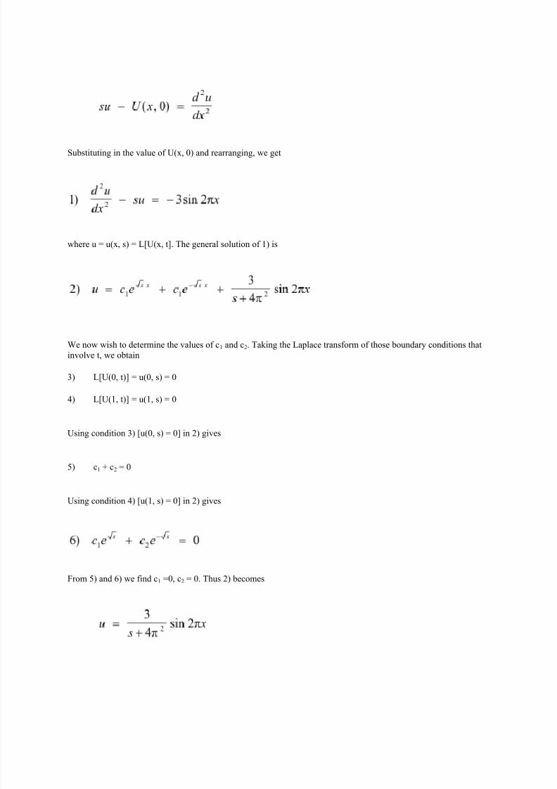
Substituting in the value of U(x, 0) and rearranging, we get

where u = u(x, s) = L[U(x, t]. The general solution of 1) is

We now wish to determine the values of c1 and c2. Taking the Laplace transform of those boundary conditions that

involve t, we obtain

3) L[U(0, t)] = u(0, s) = 0

4) L[U(1, t)] = u(1, s) = 0

Using condition 3) [u(0, s) = 0] in 2) gives

5) c1 + c2 = 0

Using condition 4) [u(1, s) = 0] in 2) gives

From 5) and 6) we find c1 =0, c2 = 0. Thus 2) becomes

7/27/2019 Laplace Transform of Partial Derivatives

http://slidepdf.com/reader/full/laplace-transform-of-partial-derivatives 6/6

 

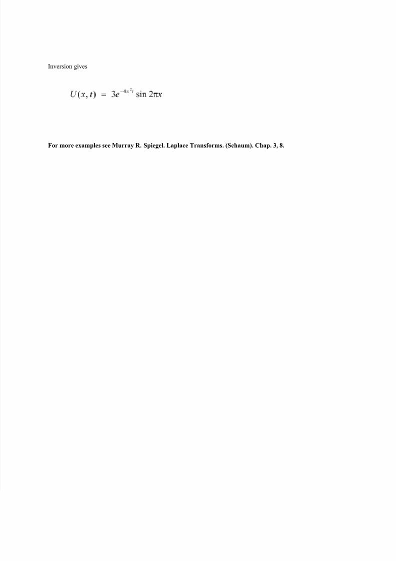
Inversion gives

For more examples see Murray R. Spiegel. Laplace Transforms. (Schaum). Chap. 3, 8.