Laplace Transform and Differential Equations
138
UNIVERSITY OF KWAZULU-NATAL Department of Mathematics at Howard College LAPLACE TRANSFORM and DIFFERENTIAL EQUATIONS 2009
-
Upload
mymydestiny -
Category
Documents
-
view
173 -
download
12
Transcript of Laplace Transform and Differential Equations
UNIVERSITY OF
KWAZULU-NATAL
Department of Mathematicsat Howard College
Le ture Notes inEngineering Mathemati s
LAPLACE TRANSFORM
and
DIFFERENTIAL
EQUATIONS
2009
Preliminaries 1
Chapter Zero
PRELIMINARIES
1. Improper Integrals
If∫ M
x0
f(x) dx exists for every M , and limM→∞∫ M
x0
f(x) dx also exists and is finite, then wedefine
∫ ∞
x0
f(x) dx = limM→∞
∫ M
x0
f(x) dx.
We also say the integral converges. It may be shown that
∣
∣
∣
∣
∫ ∞
x0
f(x) dx
∣
∣
∣
∣
≤∫ ∞
x0
|f(x)| dx;
if the integral on the right converges, then the integral on the left also converges and we say itconverges absolutely.
An absolutely convergent integral is always convergent, too; but the converse is not neces-sarily true.
To establish whether an improper integral converges or diverges, one may sometimes usethe comparison test: suppose |f(x)| ≤ |g(x)| from some point onwards (say, for x > a): then
∫ ∞
a
|f(x)| dx = ∞ =⇒∫ ∞
a
|g(x)| dx = ∞
(both integrals diverge). Vice-versa,
∫ ∞
a
|f(x)| dx < ∞ ⇐=
∫ ∞
a
|g(x)| dx < ∞
(both integrals converge absolutely). The comparison test is useful, for example, when it isrelatively easy to integrate f(x) but not g(x), or vice-versa.
2. Integration by Parts
The “product rule” for differentiation is usually written as (uv)′ = u′v + uv′. By simple manip-ulations, we get immediately
u′v = (uv)′ − uv′.
Integrating with respect to the independent variable (let us call it x), we get
∫
u′v dx = uv −∫
uv′ dx. (1)
2 Preliminaries
Using definite integration instead, we get
∫ b
a
u′v dx =[
u v]b
a−
∫ b
a
u v′ dx. (2)
Both formulas (1) and (2) are called “integration by parts”.
3. An Important Result
Observe that∫ ∞
0
e−x dx =[
− e−x]∞
0= −(0 − 1) = 1.
Then consider∫ ∞0
xe−x dx: integrating by parts, we get
∫ ∞
0
xe−x dx =[
− xe−x]∞
0−
∫ ∞
0
(
− e−x)
dx.
We need to find[
− xe−x]∞
0= lim
M→∞
[
− Me−M]
−[
− 0e−0]
=
= limM→∞
−M
eM.
The limit on the right is of the form ∞/∞, and de l’Hospital’s theorem is applicable: one getsimmediately that this limit is zero. Substituting back, it follows
∫ ∞
0
xe−x dx = 0 +
∫ ∞
0
e−x dx = 1.
In the same way, using integration by parts, we see that
∫ ∞
0
x2e−x dx = limM→∞
[
−M2
eM
]
+02
e0−
∫ ∞
0
(
− 2xe−x)
dx.
By de l’Hospital’s rule (applied twice)
limM→∞
[
−M2
eM
]
= 0;
hence∫ ∞
0
x2e−x dx = 0 + 2
∫ ∞
0
xe−x dx = 2 · 1.
More generally: if n is a positive integer, then applying de l’Hospital’s theorem n times, we mayshow that
limM→∞
Mn
eM= 0;
in other words, the exponential function eM always diverges faster than any (arbitrarily large)power Mn, as M tends to infinity. This statement remains true even if eM is replaced byeεM , where ε is positive and arbitrarily small. Exponential growth is inherently stronger thanpolynomial growth of any degree.
Preliminaries 3
Now, using these results, and repeating integration by parts n times, it is easy to see that
∫ ∞
0
xne−x dx = 0 +
∫ ∞
0
nxn−1e−x dx =
= 0 +
∫ ∞
0
n(n − 1)xn−2e−x dx =
= 0 +
∫ ∞
0
n(n − 1)(n − 2)xn−3e−x dx = etc. etc.
= n! ,
where n! = 1 · 2 · 3 · · · n.
4. Euler’s Formula
Euler studied the properties of the quantity†
w = cos φ + i sin φ,
where i2 = −1. It is easy to verify that the magnitude and argument of w are, respectively
|w| = 1, arg(w) = φ.
If two such expressions are multiplied together, one gets this identity:
(cos φ1 + i sin φ1)(cos φ2 + i sin φ2) = cos(φ1 + φ2) + i sin(φ1 + φ2)
(verify this). Following Euler, we define the exponential of an imaginary quantity in the followingway:
eiφ def= cos φ + i sin φ.
It is easy to see that this definition extends to imaginary exponentials all properties establishedfor real exponentials: for example
e−iφ =1
eiφ, eiφ1eiφ2 = ei(φ1+φ2),
d eicφ
dφ= iceicφ,
and so on. The following formulas are also very useful and should be memorized:
cos φ =eiφ + e−iφ
2sin φ =
eiφ − e−iφ
i2.
As an exercise, use Euler’s formula to derive the identities
cos A cos B = 12 [cos(A + B) + cos(A − B)], sin A cos B = 1
2 [sin(A + B) + sin(A − B)],
which you saw in high school.
† Euler did not call it a complex quantity, as we should have done, because complex numbershad not yet been properly defined. In a sense, he was ahead of his times.
4 The Laplace Transform
Chapter One
THE LAPLACE TRANSFORM
1. Introduction
Definition: Suppose f(t) is a given function of t, and the integral
∫ ∞
0
e−stf(t) dt (3)
converges for some value of the parameter s. Then the integral (3) is called the Laplace Transform
of f(t) and is denoted either as L [f(t)] or F (s).
Example 1 If f(t) = 3t + 4,
L [3t + 4] =
∫ ∞
0
(3t + 4) e−st dt.
If s > 0, by substituting st = x (so that t = +∞ corresponds to x = +∞) we get immediately
L [3t + 4] =3
s2
∫ ∞
0
xe−x dx +4
s
∫ ∞
0
e−x dx =3
s2+
4
s. [s > 0]
On the other hand, if s ≤ 0, then t = +∞ is mapped into x = −∞; we get a divergent integral,hence the Laplace transform of 3t + 4 is not defined for negative s.
Example 2 If f(t) = 7e2t, then
L[
7e2t]
=
∫ ∞
0
7e2te−st dt =
[
7e(2−s)t
2 − s
]∞
0
=7
s − 2.
Note that in this example the Laplace transform is defined only for s > 2.
Example 3 Find L [f(t)], if f(t) =(
e7t + 3)2
.
Solution: Expanding the square, we get(
e7t + 3)2
= e14t + 6e7t + 9, and hence
L [f(t)] =
∫ ∞
0
(
e14t + 6e7t + 9)
e−st dt =1
s − 14+
6
s − 7+
9
s.
Note that in this example the Laplace transform is defined only for s > 14.
The Laplace Transform 5
Example 4 Find L [f(t)], if f(t) = 2 for 4 ≤ t ≤ 7; f(t) = 0 everywhere else.
Solution: One has immediately
L [f(t)] =
∫ 7
4
2e−st dt =
[
2e−st
−s
]7
4
=2e−4s − 2e−7s
s.
Comment: A function like f(t) in this example, is called a transient because it “comes to life”,so to speak, when t = 4, at which point it jumps to the value 2 (here we have a discontinuity);when t is increased beyond the point t = 7 (another discontinuity) f(t) vanishes for good.
Before we begin to study the properties of the Laplace transform, which will take a fair amountof time, let us make some preliminary remarks.
• The integration variable is commonly called t, rather than x. This is because in mostapplications, t physically represents time. There may be exceptions to this rule.
• The Laplace transform defines a correspondence between functions of t and functions of s.Such a correspondence is a linear map: in other words, given two functions of t, f1 and f2,and two constants c1 and c2, then
L[
c1f1(t) + c2f2(t)]
= c1L[
f1(t)]
+ c2L[
f2(t)]
. (linearity)
• We assume that s is real. This keeps the foregoing discussion as simple as possible; but bewarned, certain properties of the Laplace transform are easier to study if s is treated as acomplex variable.
• If∫ ∞0
e−stf(t) dt converges absolutely for a certain s, then it converges absolutely for allvalues of s greater than that. This follows from the simple observation that if s > s0, then|e−st| < |e−s0t| for all positive t.
• If two functions, say f(t)and g(t) are identical for t ≥ 0, then clearly they have the sameLaplace transform; their behavior for negative t is irrelevant. So, with no loss of generality,we may assume f(t) = 0 identically for negative t.
• For the integral (3) to converge for some s, it is sufficient that |f(t)| be integrable to theright of the origin, and do not diverge faster than an exponential as t → ∞. We havealready noted that all powers of t, and hence all polynomials, meet this requirement.
2. Notation. Uniqueness
The function f(t) appearing in (3) is sometimes called the direct function or pre-image; thetransform itself is usually called the image of f(t).
Following an established tradition, we shall use the same letter of the alphabet for the directfunction and for its transform, with the understanding that small letters such as f , g, x, y, ωetc. will be used for direct functions, and the corresponding capital letters F , G, X, Y , Ω etc.for their transforms.† Occasionally we shall also need Greek letters for dummy variables: inthis case, recall that τ (“tau”) and σ (“sigma”) are the Greek equivalent of small t and small s,respectively.
Derivatives with respect to t will generally be denoted by dots (Newton’s notation), as it iscommon in physics and engineering. Derivatives with respect to s will be denoted by the more
† Warning: some books use small letters for transforms and capital letters for direct functions,which can be very confusing.
6 The Laplace Transform
usual primes. For example:
x =dx
dt, y =
d2y
dt2;
(FG)′′ = F ′′G + 2F ′G′ + FG′′ =d2F
ds2G + 2
dF
ds
dG
ds+ F
d2G
ds2.
We conclude these preliminaries with a rather subtle point. It is obvious that if f(t) ≡ g(t),then F (s) = G(s). But it is not obvious at all whether from F (s) = G(s) one may deduce thatf(t) = g(t) anywhere. In a sense, this is blatantly false, since f and g may take arbitrary valuesfor t < 0; and that is precisely the reason why we stipulated that direct functions be re-definedto be identically zero for negative t.
The question of equality of the original functions, when the transforms are equal, is theobject of Lerch’s theorem,† which says that under very reasonable assumptions, if F (s) = G(s)then f(t) = g(t) for all positive t, except at most a finite number of isolated points.
From the point of view of applications, Lerch’s theorem says that if F (s) = G(s) then “forall practical purposes” f(t) = g(t).
3. Basic Transforms
The following transforms must be committed to memory.
L [ect] =1
s − c[s > c] (4)
L [cosh ωt] =s
s2 − ω2[s > |ω|] (5)
L [sinhωt] =ω
s2 − ω2[s > |ω|] (6)
L [cos ωt] =s
s2 + ω2[s > 0] (7)
L [sin ωt] =ω
s2 + ω2[s > 0] (8)
L [tc] =c!
sc+1. [s > 0, c > −1] (9)
The proof of (4) is straightforward:
L [ect] =
∫ ∞
0
ecte−st dt =
[
e(c−s)t
c − s
]∞
0
= 0 − 1
c − s=
1
s − c,
as long as s > c. The proofs for (5) and (6) are corollaries:
L [cosh ωt] = L[
12
(
eωt + e−ωt)]
=1
2(s − ω)+
1
2(s + ω)=
s
s2 − ω2,
L [sinhωt] = L[
12
(
eωt − e−ωt)]
=1
2(s − ω)− 1
2(s + ω)=
ω
s2 − ω2.
In order to prove (7) and (8), we may use Euler’s formula:
eiωt = cos ωt + i sin ωt. (10)
† Matyas Lerch (1860–1922), Czech.
The Laplace Transform 7
We have then by (4):
L [eiωt] =1
s − iω=
s + iω
s2 + ω2.
Now (by definition) L [cos ωt] and L [sin ωt] are certainly real: hence, separating real and imag-inary part in the last expression, we get
L [cos ωt] = Re
[
s + iω
s2 + ω2
]
=s
s2 + ω2;
L [sin ωt] = Im
[
s + iω
s2 + ω2
]
=ω
s2 + ω2.
Example 5 Find the Laplace transform of sin3 10t.
Solution: First of all, we must put sin3 10t into a simple form, without powers. This may be doneusing the identities you learnt in high school, but perhaps the best way is by Euler’s formula(10), which gives
sin ωt =eiωt − e−iωt
i2.
It follows
sin3 10t =
(
ei10t − e−i10t
i2
)3
;
expanding the cube, we get
sin3 ωt =ei30t − 3ei10t + 3e−i10t − e−i30t
−i8=
=ei30t − e−i30t
−i4 · 2 − 3 · ei10t − e−i10t
−i4 · 2 =
= − 14
sin 30t + 34
sin 10t.
From this identity, and formula (8), we get immediately that
L[
sin3 10t]
= − 14 · 30
s2 + 900+ 3
4 · 10
s2 + 100.
Example 6 Find the Laplace transform of sin 2t cos 9t.
Solution: Simple manipulations (or Euler’s formula) give
sin 2t cos 9t = 12 sin 11t − 1
2 sin 7t;
it follows immediately that
L [sin 2t cos 9t] =11/2
s2 + 121− 7/2
s2 + 49.
The proof of (9) is bit more involved and requires a new concept, which is introduced in thenext section.
You will find that, in applications, the few basic transforms (4–9) listed above are oftenall that one needs to know. Just like we seldom calculate derivatives as a limit of the form
8 The Laplace Transform
(
f(x + h) − f(x))
/h, but rather through the rules of “differential calculus”, so there exists a“Laplace calculus” which allows us to calculate many Laplace transforms without going back tothe definition (3).
4. The Factorial Function
Consider L [tn], n being a positive integer. We substitute st with x in the integral (3) (if s ispositive, this maps t = +∞ into x = +∞), and then integrate by parts n times:
L [tn] =
∫ ∞
0
tne−st dt =1
sn+1
∫ ∞
0
xne−x dx =n!
sn+1. [s > 0]
Essentially, we have repeated the procedure outlined in section 0.3 . It works because we startedwith an integer power tn; but what about, for example,
√t, or more general powers of t? For
positive s, integrating by parts once, we get
L[√
t]
=
∫ ∞
0
t1/2e−st dt =1
s3/2
∫ ∞
0
x1/2e−x dx = 0 − 1
s3/2
∫ ∞
0
12x−1/2
(
− e−x)
dx.
The integral on the right converges, but cannot be done analytically; another round of integra-tion by parts leads nowhere, because
∫ ∞0
x−3/2e−x dx is divergent (convince yourself of this).Integration by substitution is also useless; it has been shown that there is no change of variablesthat resolves this integral as a combination of elementary functions (polynomials, sine/cosineetc.).
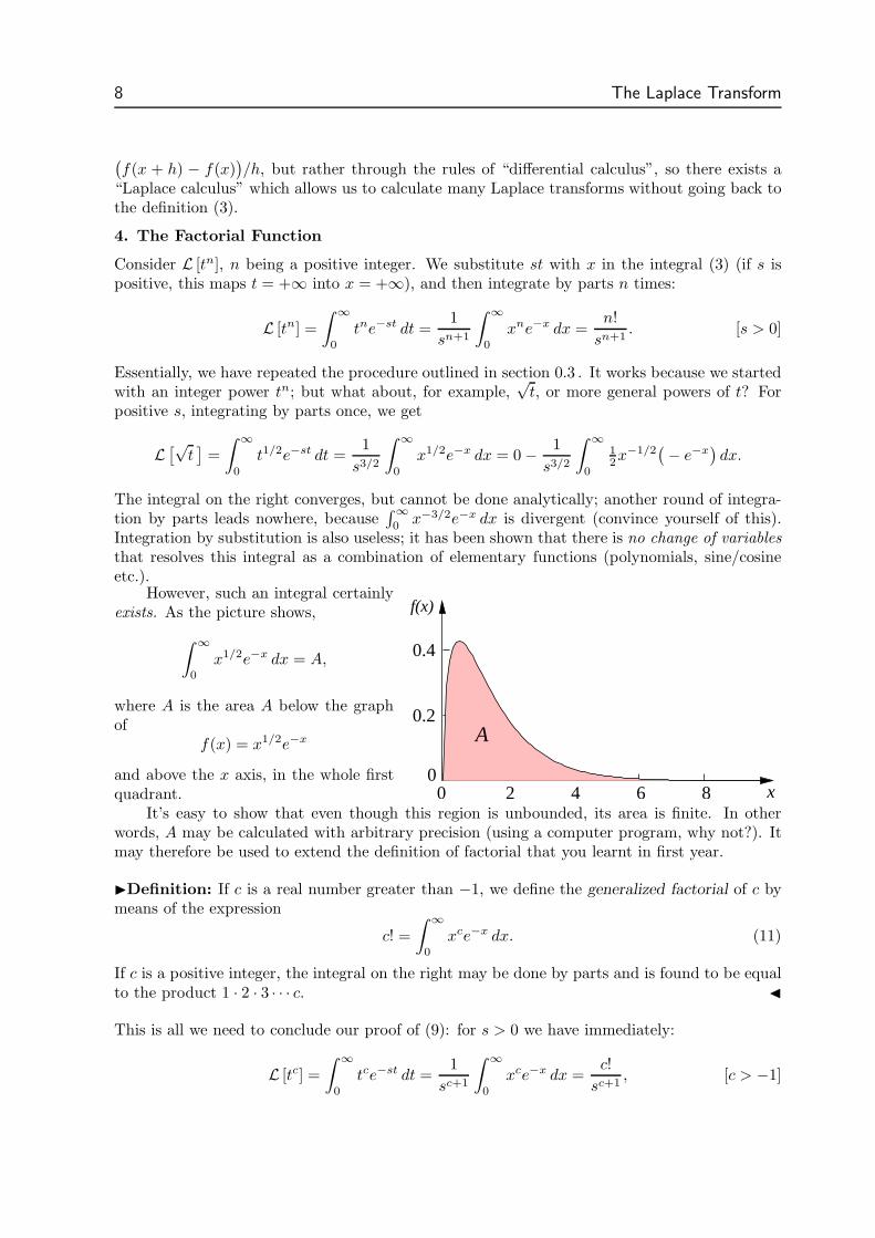
However, such an integral certainlyexists. As the picture shows,
∫ ∞
0
x1/2e−x dx = A,
where A is the area A below the graphof
f(x) = x1/2e−x
and above the x axis, in the whole firstquadrant. x
f(x)
A
2 4 6 8 0 0
0.2
0.4
It’s easy to show that even though this region is unbounded, its area is finite. In otherwords, A may be calculated with arbitrary precision (using a computer program, why not?). Itmay therefore be used to extend the definition of factorial that you learnt in first year.
Definition: If c is a real number greater than −1, we define the generalized factorial of c bymeans of the expression
c! =
∫ ∞
0
xce−x dx. (11)
If c is a positive integer, the integral on the right may be done by parts and is found to be equalto the product 1 · 2 · 3 · · · c.
This is all we need to conclude our proof of (9): for s > 0 we have immediately:
L [tc] =
∫ ∞
0
tce−st dt =1
sc+1
∫ ∞
0
xce−x dx =c!
sc+1, [c > −1]
The Laplace Transform 9
where c! is defined in (11). As an exercise, convince yourself that∫ ∞0
xce−x dx = ∞ if c ≤ −1.Factorials possess a simple and useful recursive property: if c > −1, then
(c + 1)! = (c + 1) · c! (12)
If c is a positive integer, this follows immediately from the “old” definition of factorial. If c isan arbitrary real number greater than −1, then integrating by parts we get
(c + 1)! =
∫ ∞
0
xc+1e−x dx =[
− xc+1e−x]∞
0+
∫ ∞
0
(c + 1)xce−x dx.
The integrated part is zero: by assumption c + 1 > 0, hence
limx→0
xc+1 = 0;
also (see section 0.3),lim
x→∞xc+1e−x = 0.
It follows
(c + 1)! = 0 +
∫ ∞
0
(c + 1)xce−x dx = (c + 1) · c! ,
which is (12), as required to prove.An important consequence of (12) is that once a table of generalized factorials has been
calculated for any interval of unit length, it may be extended outside such an interval usingordinary multiplications.
Example 7 Calculate 5.3273! , assuming that a table of c! is available only for 0 ≤ c ≤ 1.
Solution: By (12), we may write 5.3273! = 5.3273 . 4.3273!. Repeating this procedure four moretimes, we get
5.3273! = 5.3273 . 4.3273 . 3.3273 . 2.3273 . 1.3273 . 0.3273!
and at this point we look up 0.3273! in the table. There, we find that 0.3273! ≈ 0.89371; therefore5.3273! ≈ 211.7553, which lies between 5! = 120 and 6! = 720.
We told you a half-lie. You probably thought that the only case when c! may be calculated in aneasy way, is if c is a positive integer or zero. Whether this statement is true or false, depends onwhat you mean by “easy”. As it happens, using the Laplace transform it is possible to calculatec! when c is half-odd; we shall come back to this in chapter 2, where it is shown that
(− 12)! =
√π.
From this, one gets immediately, using (12):
12 ! = 1
2 · (− 12 )! = 1
2
√π
32 ! = 3
2 · 12 ! = 3
4
√π
52! = 5
2· 3
2! = 15
8
√π
72 ! = 7
2 · 52 ! = 105
16
√π
92 ! = etc.
10 The Laplace Transform
Finally, a word of warning. Most books still introduce generalized factorials by means of Legen-dre’s so-called “gamma function”; that is, they write Γ(c+1) for c! . That extra +1 is there onlyfor historical reasons, and is as necessary as the human appendix.† Today, as the best computerprograms (such as maxima, maple, mathematica, etc.) accept both notations, there is noneed for us to persist with the bulkier gamma notation. Most important, the exclamation markis a good reminder of the link with “ordinary” factorials.
5. Basic Properties; Multiplication by s
Before we begin to study the analytic properties of the Laplace transform, we must make someassumptions on the function f(t) that appears in the definition (3). Clearly, it is not necessarythat f(t) be continuous for the integral in (3) to converge: the function in example 4, for instance,is discontinuous. On the other hand, it is easy to produce functions with no Laplace transformfor any value of s: for example, f(t) = et2 or f(t) = 1/t.
There is no special term in the mathematical literature describing “a function that admitsa Laplace transform”, but we can easily do without it. However, we introduce now a couple ofdefinitions that will help us through our discussion.
Definition: A function f(t) is said to be sectionally continuous if it is continuous everywhereexcept at a finite number of discontinuities, and at each point of discontinuity both the limitfrom the right and the limit from the left, of f(t), exist and are finite.
Example 8 Let f(t) = t for t ∈ [0, 1]; f(t) = t2 for t ∈ (1,∞). Then f(t) is continuousfor every t; f(t) is only sectionally continuous, because f(t) = 1 in (0, 1), f(t) = 2t in (1,∞),limt→1− f(t) = 1, limt→1+ f(t) = 2. At t = 1, which is a point of discontinuity, the limit fromthe left and the limit from the right of f are different, but both are finite.
Definition: A function f(t) is of exponential order if there exist two positive constants c andB such that |f(t)| < B ect, for all t from a certain point onwards.
These definitions are broad enough to include most functions of practical relevance. Clearly, ifa function is sectionally continuous and of exponential order, then the integral in (3) converges,and hence its Laplace transform exists—for sufficiently large s, possibly.
It also follows that, if f(t) is of exponential order, and s is large enough, then
limt→∞
|f(t)|e−st = 0
(i.e., this is true for all s greater than some constant γ).Suppose now that f(t), f(t) are of exponential order; f(t) is continuous and f(t) sectionally
continuous. By definition,
L [f(t)] =
∫ ∞
0
(df/dt) e−st dt.
Integrating by parts, we get
L [f(t)] =[
f(t) e−st]∞
0−
∫ ∞
0
f(t)(−se−st ) dt.
† Quoted from G. Arfken, Mathematical Methods for Physicists, Wiley (USA) 1970.
The Laplace Transform 11
This may also be written:
L [f(t)] = limt→∞
f(t) e−st − limt→0+
f(t) e−st + s
∫ ∞
0
f(t) e−st dt.
Since we assume that f(t) is of exponential order, the first of the limits above is zero (for suffi-ciently large s). The second limit is equal to limt→0+ f(t), i.e., the limit of f(t) as t approacheszero from the right—remember, by definition f(t) ≡ 0 if t is negative. We write
limt→0+
f(t) = f0.
It follows immediately thatL [f(t)] = −f0 + sF (s). (13)
Example 9 Find the function x(t) such that 5x + 3x = 0 and x0 = 2.
Solution: We take the Laplace transform of the equation. We get
L [5x + 3x] = 0,
where L [x] = X(s), and L [x] = −x0 + sX(s) = −2 + sX(s). It follows
5(−2 + sX) + 3X = 0,
which yields
X =10
5s + 3=
2
s + 3/5.
Now, by inspection, we recognize that
1
s + 3/5= L
[
e−3t/5]
;
Therefore, it follows immediately that
X = L[
2e−3t/5]
,
and finally (by Lerch’s theorem) x = 2e−3t/5.
Transforms of higher-order derivatives may be calculated by repeated application of (13). Forexample, if f and f are continuous, and f is sectionally continuous, then
L [f(t)] = −f0 + sL [f(t)],
where f0 denotes limt→0+ f(t). Substituting for L [f(t)] its expression (13), we get
L [f(t)] = −f0 + s(−f0 + sF (s)) =
= −f0 − sf0 + s2F (s). (14)
12 The Laplace Transform
Similarly,
L[ ˙f(t)
]
= −f0 + sL [f(t)]) =
= −f0 − sf0 − s2f0 + s3F (s), (15)
where f0 denotes limt→0+ f(t). Naturally, here, we must assume that f , f and f are continuous,and the third derivative of f(t) is sectionally continuous.
Formulas for higher-order derivatives may be calculated in the same way, if needed. How-ever, in each case, the assumptions must be extended: the highest derivative of f(t) must besectionally continuous, and all lower-order derivatives (including f) must be continuous. Intypical engineering applications, these assumptions are generally satisfied.
Example 10 Calculate L[
cos2 t]
with and without (13).
Solution: Without using (13), one may find L[
cos2 t]
using the identity cos2 t = 12 (cos 2t + 1).
This gives
L [cos2 t] = 12L [cos 2t] + 1
2L [1]
= 12 ·
(
s
s2 + 4+
1
s
)
.
In order to use (13), we first note that f0 = 1 and f = −2 sin t cos t = − sin 2t. It then followsthat
L [f ] = − 2
s2 + 4,
and, by (13), that
L [f ] = sL [cos2 t] − 1.
By comparison, one gets that
sL [cos2 t] − 1 = − 2
s2 + 4,
which finally yields
L [cos2 t] =1
s− 2
s(s2 + 4).
Since
12 ·
(
s
s2 + 4+
1
s
)
=s2 + 2
s(s2 + 4)=
1
s− 2
s(s2 + 4),
the two results are identical.
This example works because cos2 t is continuous throughout, and so are its derivatives of anyorder. But the continuity requirements are crucial, as the following example shows.
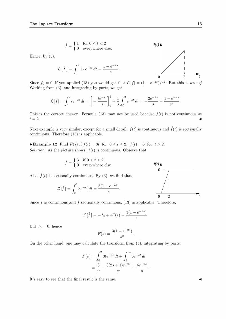
Example 11 Find F (s), if f(t) = t for 0 ≤ t < 2, and f(t) = 0 everywhere else.
Solution: Before we start: if you apply (13), you get the wrong answer. Let us see why. Thegraph of f(t) is pictured on the right; note the discontinuity at t = 2. It follows that
The Laplace Transform 13
f =
1 for 0 ≤ t < 20 everywhere else.
Hence, by (3),
L[
f]
=
∫ 2
0
1 · e−st dt =1 − e−2s
s.
t
f(t)
20
Since f0 = 0, if you applied (13) you would get that L [f ] = (1 − e−2s)/s2. But this is wrong!Working from (3), and integrating by parts, we get
L [f ] =
∫ 2
0
te−st dt =
[
− te−st
s
]2
0
+1
s
∫ 2
0
e−st dt = −2e−2s
s+
1 − e−2s
s2.
This is the correct answer. Formula (13) may not be used because f(t) is not continuous att = 2.
Next example is very similar, except for a small detail: f(t) is continuous and f(t) is sectionallycontinuous. Therefore (13) is applicable.
Example 12 Find F (s) if f(t) = 3t for 0 ≤ t ≤ 2; f(t) = 6 for t > 2.
Solution: As the picture shows, f(t) is continuous. Observe that
f =
3 if 0 ≤ t ≤ 20 everywhere else.
Also, f(t) is sectionally continuous. By (3), we find that
L [f ] =
∫ 2
0
3e−st dt =3(1 − e−2s)
s.
t20
f(t)6
Since f is continuous and f sectionally continuous, (13) is applicable. Therefore,
L [f ] = −f0 + sF (s) =3(1 − e−2s)
s.
But f0 = 0, hence
F (s) =3(1 − e−2s)
s2.
On the other hand, one may calculate the transform from (3), integrating by parts:
F (s) =
∫ 2
0
3te−st dt +
∫ ∞
2
6e−st dt
=3
s2− 3(2s + 1)e−2s
s2+
6e−2s
s.
It’s easy to see that the final result is the same.
14 The Laplace Transform
6. Division by s
It follows from the fundamental theorem of calculus that
d
dt
∫ t
0
f(τ) dτ = f(t).
The integral on the left-hand side is an anti-derivative of f(t)†. We now call it g:
g(t)def=
∫ t
0
f(τ) dτ,
and observe thatg(t) = f(t), g(0+) = 0.
Taking the Laplace transform of the identity
L [g(t)] = L [f(t)]
and using (13), we get−g0 + sG(s) = F (s).
But g0 = 0. Hence,
G(s) =F (s)
s,
which may finally be expanded as
L[
∫ t
0
f(τ) dτ
]
=F (s)
s. (16)
Naturally, this formula may be iterated any number of times. For example, if we integratebetween zero and t the function g defined at the beginning of this section, we get another functionof t, let us call it h, such that h(t) = f(t), and h(0) = h(0) = 0; therefore L [h(t)] = F (s)/s2.
Then, integrating h between zero and t and reasoning in the same way, we obtain yetanother function of t, and its Laplace transform will be F (s)/s3. And so on: the process maybe repeated as many times as needed.
Example 13 Find the function x(t) such that 2x + 4x = 2 and x0 = 1.
Solution: We take the Laplace transform of the equation. We get
L [2x + 4x] = L [2],
where L [x] = X(s), L [x] = −x0 + sX(s) = −1 + sX(s), and L [2] = 2/s. It follows
2(−1 + sX) + 4X =2
s,
† Be careful: the dummy variable of integration must not be t, because it appears as a limitof integration.
The Laplace Transform 15
which—solving for X—yields
X =1
2s + 4
(
2 +2
s
)
=1
s + 2+
1
s(s + 2).
Now, by inspection, we recognize that
1
s + 2= L
[
e−2t]
;
the second term may be simplified by rule (16):
1
s(s + 2)= L
[∫ t
0
e−2τ dτ
]
= L[
12− 1
2e−2t
]
.
Combining the two terms, it follows immediately that
X = L[
e−2t]
+ L[
12 − 1
2e−2t]
= L[
12 + 1
2e−2t]
,
and finally (by Lerch’s theorem) x = 12 + 1
2e−2t.
Example 14 Since
tn =
∫ t
0
nτn−1 dt,
we get immediately
L [tn] =nL [tn−1]
s.
In this way, starting from
L [1] =
∫ ∞
0
e−st dt =1
s,
we get
L [t] =1
s2, L [t2] =
2!
s3, L [t3] =
3!
s4, L [t4] =
4!
s5,
and so on. We recover (9), though for integer powers only.
These transforms may also be understood in terms of convolution, a more advanced techniquethat we’ll study is section 2.7.
7. Multiplication by t
It may be shown that if the integral (3) converges absolutely, then F (s) may be differentiatedany number of times with respect to s. For example,
F ′(s) =d
ds
∫ ∞
0
f(t) e−st dt =
∫ ∞
0
∂
∂s
[
f(t) e−st]
dt = −∫ ∞
0
f(t) te−st dt.
Repeating this process n times, we obtain
L [tnf(t)] = (−1)n dnF (s)
dsn. (17)
Example 15 Find L [t cosh 4t].
Solution: Since L [cosh 4t] = s/(s2 − 16), then by (17)
L [t cosh 4t] = − d
ds
s
s2 − 16= − 1
s2 − 16+
2s2
(s2 − 16)2=
s2 + 16
(s2 − 16)2.
As an exercise, calculate∫ ∞0
t cosh 4t e−st dt (integrating by parts) and verify that you get thesame answer.
16 The Laplace Transform
Example 16 Find L [t4ect].
Solution: We have from (4): L [ect] = 1/(s − c). Hence, by (17):
L [t4ect] =(
− d
ds
)4 1
s − c=
4!
(s − c)5.
Example 17 Find L [teiωt] and hence L [t cos ωt], L [t sin ωt].
Solution: From (4) we get L [eiωt] = 1/(s − iω). It follows
L [teiωt] = − d
ds
1
s − iω=
1
(s − iω)2=
(s + iω)2
(s2 + ω2)2=
s2 + i2sω − ω2
(s2 + ω2)2.
Separating real and imaginary parts, it follows immediately
L [t cos ωt] =s2 − ω2
(s2 + ω2)2;
L [t sin ωt] =2sω
(s2 + ω2)2.
As an exercise, calculate from first principles∫ ∞0
e−stt cos ωt dt or∫ ∞0
e−stt sin ωt dt, and verifythat you get the same results.
Example 18 Find the function x(t) such that 2x + x = t3e−t/2, and x0 = 0.
Solution: Taking the Laplace transform of the equation, we get
2L [x] + L [x] = L[
t3e−t/2]
.
writing L [x] = X and using (13) we get immediately
L [x] = −x0 + sX = sX.
Then, we note that
L[
e−t/2]
=1
s + 1/2=⇒ L
[
t3e−t/2]
= − d3
dt3
(
1
s + 1/2
)
=3!
(s + 1/2)4;
this step (multiplication by t3) follows from (17). Substituting these expressions into the pre-ceding equation yields:
2sX + X =6
(s + 1/2)4.
Hence
X =6
(2s + 1)(s + 1/2)4=
3
(s + 1/2)5.
Now, we observe thatd4
dt4
(
1
s + 1/2
)
=4!
(s + 1/2)5;
The Laplace Transform 17
therefore,3
(s + 1/2)5=
3
4!
d4
dt4
(
1
s + 1/2
)
= 18 L
[
t4e−t/2]
;
this step (multiplication by t4) also follows from (17). Hence,
X = L[
18 t4e−t/2
]
,
and finally, by Lerch’s theorem,x = 1
8t4e−t/2
is the required function.
8. Division by t
If f(t) is of exponential order, then certainly
lims→∞
∫ ∞
0
|f(t)| e−st dt = 0.
In other words, if a function of s does not approach zero as s → ∞, then it is not a Laplacetransform, in the ordinary sense of the word.†
Given a function f(t) with a Laplace transform F (s), we introduce
G(s)def=
∫ ∞
s
F (σ) dσ.
Note that σ is a dummy variable; s is the lower limit of integration and we treat it as a parameter.Convince yourself that this integral is defined in such a way that if s → ∞, then G(s) tends tozero. Therefore, G(s) may be the Laplace transform of some function g(t).
By the fundamental theorem of calculus, G(s) is an anti-derivative of −F (s):
G′(s) = −F (s) = −L [f(t)].
On the other hand, it follows from (17) that
G′(s) = L [−tg(t)].
By comparison, we get f(t) = tg(t), which may be written
g(t) =f(t)
t.
Finally, tranforming again, we get G(s) = L [f(t)/t], which may be expanded as
L[
f(t)
t
]
=
∫ ∞
s
F (σ) dσ. (18)
† This comment does not apply to “generalized functions”, which you’ll find in more advancedcourses. But generalized functions are not functions in the usual sense of the word.
18 The Laplace Transform
Example 19 Find L [sin t/t].
Solution: From (8) we get L [sin t] = 1/(s2 + 1). Hence, it follows from (18) that
L[
sin t
t
]
=
∫ ∞
s
dσ
σ2 + 1=
[
arctan σ]∞
s= 1
2π − arctan s = arccot s.
Comment: By definition, L [sin t/t] =∫ ∞0
(sin t/t) e−st dt. So, we get the interesting result
∫ ∞
0
sin t
te−st dt = 1
2π − arctan s. [s > 0]
For example, for s = 1 we get∫ ∞0
(e−t sin t/t) dt = 12π − arctan 1 = 1
4π. Letting s → 0+ we get
∫ ∞
0
sin t
tdt = 1
2π,
which is a famous example of a convergent improper integral that is not absolutely convergent.Note also that these integrals may not be done using elementary calculus, as the anti-derivativesmay not be written in terms of elementary functions. We find the surprising result that definiteintegration is elementary while indefinite integration is not.
Example 20 Using the result of example 19, find G(s), given that g(t) =∫ t
0(sin τ/τ) dτ .
Solution: In example 19 we established that
L[
sin t
t
]
= arccot s.
Hence, applying (16) we get immediately that
L[
∫ t
0
sin τ
τdτ
]
=arccot s
s.
Comment: the function g(t) =∫ t
0(sin τ/τ) dτ is called integral sine, denoted si(t), and is used
in many engineering applications.
Example 21 Find L [(et − 1)/t].
Solution: From (4) and (9) we get, respectively, L [et] = 1/(s− 1) and L [1] = 1/s. It followsthat
L[
et − 1
t
]
=
∫ ∞
s
(
1
σ − 1− 1
σ
)
dσ =
=
[
ln
(
σ − 1
σ
)]∞
s
= ln 1 − lns − 1
s= ln
s
s − 1.
Again, although the indefinite integral∫ ∞0
(
e−st(et−1)/t)
dt cannot be done in closed form, theLaplace transform has been found by means of (18).
In principle, rule (18) may be iterated: division of f(t) by t2 corresponds to integrating F (s)twice, and so on. In practice, examples of this kind are likely to be fairly long. You may find
The Laplace Transform 19
one at the end of this chapter (see section 1.11). Next example shows how double integrationmay, in some cases, be avoided.
Example 22 Find the Laplace transform of sin2 t/t and hence the Laplace transform ofsin2 t/t2.
Solution: The first half of this problem is very simple: from the identity
sin2 t = 12 (1 − cos 2t)
we get immediately that
L[
sin2 t]
=1
2
(
1
s− s
s2 + 4
)
,
and hence that
L[
sin2 t
t
]
=1
2
∫ ∞
s
(
1
σ− σ
σ2 + 4
)
dσ = 12
ln
√s2 + 4
s.
Naturally, for this step we applied equation (18). For the second part, we could use (18) again,but the following shortcut is better. If we define
f(t) =sin2 t
t:
then the preceding result may be written
F (s) = 12
ln
√s2 + 4
s.
Differentiating f(t) we get that
f =2 sin t cos t
t− sin2 t
t2=
sin 2t
t− sin2 t
t2;
Note that f(0+) = 0. It follows that
sin2 t
t2=
sin 2t
t− f
and hence, by (13), that
L[
sin2 t
t2
]
= L[
sin 2t
t
]
−(
s F (s) − f(0+))
= L[
sin 2t
t
]
− 12s ln
√s2 + 4
s.
The first term on the right-hand side is almost identical to what we found in example 19:
L[
sin 2t
t
]
= arccot(s/2).
So, finally, we get:
L[
sin2 t
t2
]
= arccot(s/2) − 12s ln
√s2 + 4
s.
20 The Laplace Transform
OVERVIEW
The rules discussed in sections 5–8 may, at first, seem hard to grasp. They are not: let us putthem all together in a table.
f(t) F (s)
f(t) sF (s) − f0
∫ t
0
f(τ) dτF (s)
s
t f(t) −F ′(s)
f(t)
t
∫ ∞
s
F (σ) dσ
The first line is simply a reminder that we use lower-case letter to denote functions of t, and thecorresponding upper-case letters to denote their transforms.
You should be able to spot the thread linking the other formulas: Differentiation withrespect to one variable, t or s, is associated with multiplication by the other; integration withrespect to one variable is associated with division by the other.
We are slightly over-simplifying, now; some fine points must also be borne in mind. Forexample, integration with respect to s ends at infinity, whereas integration with respect to tstarts at zero. The rule for L [f ] must account for the possibility that f(t) be discontinuous att = 0, hence f0 appears in the second line; on the other hand, the rule for F ′(s) has a minussign, which should not be overlooked.
However, the common thread (in italics above) is easy to remember. Using the six basictransforms (4–9) as building blocks and combining the rules above, one may derive a wide varietyof transforms, with no direct call for integral calculus. We now complement this table with twomore basic rules: the shift rules.
9. Shifting s
Consider a function f(t) with Laplace transform F (s). Let α be a constant. By definition,
L[
e−αtf(t)]
=
∫ ∞
0
f(t) e−αt e−st dt.
It follows immediately
L[
e−αt f(t)]
=
∫ ∞
0
f(t) e(−s−α)t dt =
= F (s + α). (19)
Example 23 Find L[
e−4t√
t]
.
Solution: By (9) we get that[√
t]
= (1/2)!/
s3/2. Therefore, L[
e−4t√
t]
= (1/2)!/
(s + 4)3/2.
Example 24 Find L[
e−5t cos 3t]
.
Solution: Since L [cos 3t] = s/(s2 + 9), we get immediately that
L[
e−5t cos 3t]
=s + 5
(s + 5)2 + 9=
s + 5
s2 + 10s + 34.
The Laplace Transform 21
Example 25 Find L[
t3e2t]
.
Solution: Since L [t3] = 6/s4, we get immediately by (19) that
L[
t3e2t]
=6
(s − 2)4.
Note, however, that one may also start from L [e2t] = 1/(s − 2) and apply (17) three times:
L[
t3e2t]
= − d3
ds3
(
1
s − 2
)
=6
(s − 2)4.
Example 26 Find L [sin 2t cosh 3t].
Solution: By definition,
sin 2t cosh 3t = sin 2t ·(
e3t + e−3t
2
)
=
= 12e3t sin 2t + 1
2e−3t sin 2t.
It follows immediately that
L [sin 2t cosh 3t] =1
(s − 3)2 + 4+
1
(s + 3)2 + 4
Example 27 Find F (s), if f(t) = t−1∫ t
0e−3τ sin τ dτ .
Solution: We observe that f(t) is obtained by performing three operations on the function sin t,which are:
(i) multiplication by e−3t,(ii) integration with respect to t,(iii) division by t.
The corresponding operations on F (s) are:
(i) shift by 3 units to the left(ii) division by s,(iii) integration with respect to s.
Proceeding along these lines, we get:
L [sin t] =1
s2 + 1,
L[
e−3t sin t]
=1
(s + 3)2 + 1,(i)
L[∫ t
0
e−3τ sin τ dτ
]
=1
s[(s + 3)2 + 1],(ii)
and finally:
(iii) F (s) = L[
1
t
∫ t
0
e−3τ sin τ dτ
]
=
∫ ∞
s
dσ
σ[(σ + 3)2 + 1].
22 The Laplace Transform
A simple substitution yields
∫ ∞
s
dσ
σ[(σ + 3)2 + 1]=
∫ ∞
s+3
dx
(x − 3)(x2 + 1).
It is possible to show that
1
(x − 3)(x2 + 1)=
110
x − 3−
110 (x + 3)
x2 + 1,
as you can easily verify. The expansion above may be done by the methods you learnt in firstyear, but we’ll come back to this subject in the next chapter.
So, integrating, we get:
F (s) =1
10
∫ ∞
s+3
[
1
x − 3− x + 3
x2 + 1
]
dx =
=1
10
[
ln |x − 3| − 12 ln |x2 + 1| − 3 arctan x
]∞
s+3=
=1
10
[
ln
∣
∣
∣
∣
x − 3√x2 + 1
∣
∣
∣
∣
− 3 arctan x
]∞
s+3
=
=1
10
[
ln 1 − 3 · π
2− ln
s√
(s + 3)2 + 1+ 3arctan(s + 3)
]
.
Simplifying, we find that
F (s) = 110 ln
√
(s + 3)2 + 1
s− 3
10 arccot(s + 3).
10. Shifting t
We have discussed the the effects of a shift of the s axis. A shift of the t axis may be studied ina similar way.
This may be useful, for instance, if the function f(t) is defined by different formulas overdifferent pieces of the t axis. In such a case, the following approach may be useful. Suppose
f(t) =
0 if t < T ,φ(t − T ) if t ≥ T ,
where φ(t) is a function of t having Laplace transform Φ(s). Then, by definition,
F (s) =
∫ T
0
f(t) e−st dt +
∫ ∞
T
f(t) e−st dt =
= 0 +
∫ ∞
T
φ(t − T ) e−st dt.
Substituting t = T + τ , we get
F (s) =
∫ ∞
0
φ(τ)e−sT−sτ dτ =
= e−sT Φ(s). (20)
The Laplace Transform 23
Example 28 Find L [f(t)], if f(t) =
0 if t < 3,sin 2t if t ≥ 3.
Solution: We may not apply rule (20) as long as f(t) is written in this way, because the depen-dence on t − 3 is not explicit. To make it so, we manipulate the function slightly:
sin 2t = sin 2(t − 3 + 3) = sin 2(t − 3) · cos 6 + cos 2(t − 3) · sin 6.
Then we define a function
φ(t)def= sin 2t cos 6 + cos 2t sin 6,
which has the Laplace transform
Φ(s) =2 cos 6
s2 + 4+
s sin 6
s2 + 4.
Since obviouslysin 2t = φ(t − 3),
i.e.,
f(t) =
0 if t < 3,φ(t − 3) if t ≥ 3,
we are in a position to apply (20). It follows that
F (s) =e−3s(2 cos 6 + s sin 6)
s2 + 4.
In most applications, rule (20) is combined with a simple and useful mathematical tool: the stepfunction.
Definition: The function u(t), which is defined as
u(t) =
0 for negative t12 for t = 01 for positive t
is called the unit step function, or also Heaviside’s function.
Do not worry about the definition of u(t) for t = 0: it is purely conventional and does not affectthe Laplace transform in any way. It finds its place in more advanced topics.
Heaviside’s function jumps from 0 to 1 when its argument is increased across zero. So, forexample, what is u(t − 74)? Since t − 74 < 0 when t < 74, and t − 74 > 0 when t > 74, wesee that u(t − 74) jumps from 0 to 1 as t is increased across the point t = 74. By rule (20), theLaplace transform of this function would be simply
F (s) = e−74s · L [1] =e−74s
s.
Very often two step functions are combined to form a function that is zero for t up to a certainpoint, and becomes zero again from another point onwards.
24 The Laplace Transform
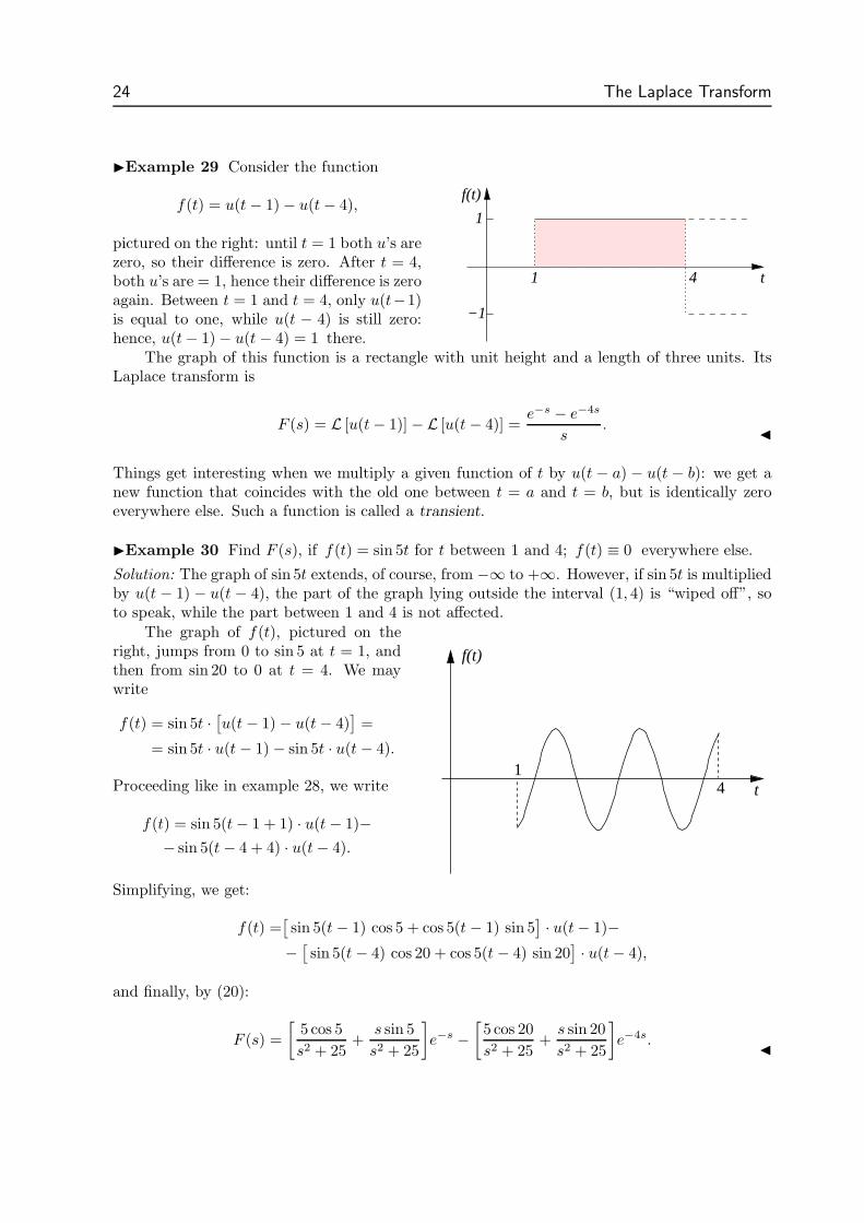
Example 29 Consider the function
f(t) = u(t − 1) − u(t − 4),
pictured on the right: until t = 1 both u’s arezero, so their difference is zero. After t = 4,both u’s are = 1, hence their difference is zeroagain. Between t = 1 and t = 4, only u(t−1)is equal to one, while u(t − 4) is still zero:hence, u(t − 1) − u(t − 4) = 1 there.
t
1
−1
1 4
f(t)
The graph of this function is a rectangle with unit height and a length of three units. ItsLaplace transform is
F (s) = L [u(t − 1)] − L [u(t − 4)] =e−s − e−4s
s.
Things get interesting when we multiply a given function of t by u(t − a) − u(t − b): we get anew function that coincides with the old one between t = a and t = b, but is identically zeroeverywhere else. Such a function is called a transient.
Example 30 Find F (s), if f(t) = sin 5t for t between 1 and 4; f(t) ≡ 0 everywhere else.
Solution: The graph of sin 5t extends, of course, from −∞ to +∞. However, if sin 5t is multipliedby u(t − 1) − u(t − 4), the part of the graph lying outside the interval (1, 4) is “wiped off”, soto speak, while the part between 1 and 4 is not affected.
The graph of f(t), pictured on theright, jumps from 0 to sin 5 at t = 1, andthen from sin 20 to 0 at t = 4. We maywrite
f(t) = sin 5t ·[
u(t − 1) − u(t − 4)]
=
= sin 5t · u(t − 1) − sin 5t · u(t − 4).
Proceeding like in example 28, we write
f(t) = sin 5(t − 1 + 1) · u(t − 1)−− sin 5(t − 4 + 4) · u(t − 4).
t1
4
f(t)
Simplifying, we get:
f(t) =[
sin 5(t − 1) cos 5 + cos 5(t − 1) sin 5]
· u(t − 1)−−
[
sin 5(t − 4) cos 20 + cos 5(t − 4) sin 20]
· u(t − 4),
and finally, by (20):
F (s) =
[
5 cos 5
s2 + 25+
s sin 5
s2 + 25
]
e−s −[
5 cos 20
s2 + 25+
s sin 20
s2 + 25
]
e−4s.
The Laplace Transform 25
It should be noted that problems of this type may always be done from first principles. However,with some practice you’ll find that the method of this section is usually better. For instance,the last example may also be done by calculating
F (s) =
∫ 4
1
e−st sin 5t dt
using integration by parts or Euler’s formula. Do it, as an exercise.
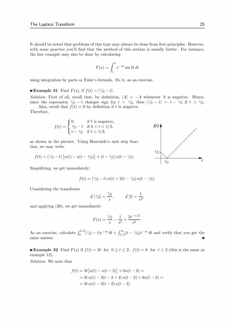
Example 31 Find F (s), if f(t) =∣
∣1/2 − t∣
∣.
Solution: First of all, recall that, by definition, |A| = −A whenever A is negative. Hence,since the expression 1/2 − t changes sign for t = 1/2, then |1/2 − t| = t − 1/2 if t > 1/2.
Also, recall that f(t) ≡ 0 by definition if t is negative.Therefore,
f(t) =
0 if t is negative,1/2 − t if 0 < t < 1/2,t − 1/2 if t > 1/2,
as shown in the picture. Using Heaviside’s unit step func-tion, we may write
f(t) = (1/2 − t)[
u(t) − u(t − 1/2)]
+ (t − 1/2)u(t − 1/2).
/1 2
/1 2
f(t)
t
Simplifying, we get immediately:
f(t) = (1/2 − t)u(t) + 2(t − 1/2)u(t − 1/2).
Considering the transforms
L [1/2] =1/2s
, L [t] =1
s2,
and applying (20), we get immediately
F (s) =1/2s
− 1
s2+
2e−s/2
s2.
As an exercise, calculate∫ 1/2
0(1/2 − t)e−st dt +
∫ ∞1/2
(t − 1/2)e−st dt and verify that you get thesame answer.
Example 32 Find F (s) if f(t) = 3t for 0 ≤ t ≤ 2; f(t) = 6 for t > 2 (this is the same asexample 12).
Solution: We note that
f(t) = 3t[
u(t) − u(t − 2)]
+ 6u(t − 2) =
= 3t u(t) − 3(t − 2 + 2)u(t − 2) + 6u(t − 2) =
= 3t u(t) − 3(t − 2)u(t − 2).
26 The Laplace Transform
It follows immediately that
F (s) =3
s2− 3e−2s
s2:
same result as in example 12.
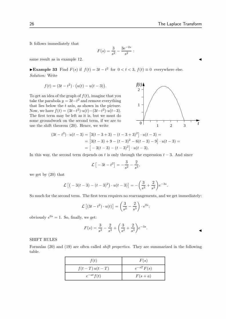
Example 33 Find F (s) if f(t) = 3t − t2 for 0 < t < 3, f(t) ≡ 0 everywhere else.
Solution: Write
f(t) = (3t − t2) ·(
u(t) − u(t − 3))
.
To get an idea of the graph of f(t), imagine that youtake the parabola y = 3t−t2 and remove everythingthat lies below the t axis, as shown in the picture.Now, we have f(t) = (3t−t2)·u(t)−(3t−t2)·u(t−3).The first term may be left as it is, but we must dosome groundwork on the second term, if we are touse the shift theorem (20). Hence, we write
t
f(t)
1
2
1 2 3 0
(3t − t2) · u(t − 3) =[
3(t − 3 + 3) − (t − 3 + 3)2]
· u(t − 3) =
=[
3(t − 3) + 9 − (t − 3)2 − 6(t − 3) − 9]
· u(t − 3) =
=[
− 3(t − 3) − (t − 3)2]
· u(t − 3).
In this way, the second term depends on t is only through the expression t − 3. And since
L[
− 3t − t2]
= − 3
s2− 2
s3,
we get by (20) that
L[(
− 3(t − 3) − (t − 3)2)
· u(t − 3)]
= −(
3
s2+
2
s3
)
e−3s.
So much for the second term. The first term requires no rearrangements, and we get immediately:
L[
(3t − t2) · u(t)]
=
(
3
s2− 2
s3
)
· e0s;
obviously e0s = 1. So, finally, we get:
F (s) =3
s2− 2
s3+
(
3
s2+
2
s3
)
e−3s.
SHIFT RULES
Formulas (20) and (19) are often called shift properties. They are summarized in the followingtable.
f(t) F (s)
f(t − T )u(t − T ) e−sT F (s)
e−atf(t) F (s + a)
The Laplace Transform 27
11. Additional Examples
As a rule, the linearity property
L [f1 + f2] = L [f1] + L [f2]
holds only if L [f1] and L [f2] exist each one on its own. It may happen, though, that the Laplacetransform of f1 + f2 does exist, even if f1 and f2 do not have a Laplace transform.
Example 34 Find F (s), if f(t) = (et − 1) · t−3/2.
Solution: We would like to use the shift theorem (19). However,
∫ ∞
0
ett−3/2e−st dt −∫ ∞
0
t−3/2e−st dt = ∞−∞
which is clearly meaningless. So, F (s) may not be “split” as we did in several previous examples;see for instance example 26.
On the other hand, it’s easy to see that F (s) exists, and we are going to find it in two steps.First of all we write
g(t) =et − 1
t1/2, f(t) =
et − 1
t3/2=
g(t)
t,
and consider G(s). This is easy, because L[
ett−1/2]
and L[
t−1/2]
exist separately:
L[
t−1/2]
=(−1/2)!
s1/2, L
[
ett−1/2]
=(−1/2)!
(s − 1)1/2;
the second one comes via the shift theorem (19). Therefore,
G(s) =(−1/2)!
(s − 1)1/2− (−1/2)!
s1/2.
Finally, we go back to f(t) and use (18)—division by t corresponds to integration by s:
F (s) =
∫ ∞
s
[
(−1/2)!
(σ − 1)1/2− (−1/2)!
σ1/2
]
dσ =
= (−1/2)!
[
(σ − 1)1/2
1/2− σ1/2
1/2
]∞
s
We should show that, in the equation above, the last expression in square brackets goes to zeroas σ tends to infinity; this is a good revision example in 1st-year calculus. Writing
(σ − 1)1/2
1/2− σ1/2
1/2=
(σ − 1)1/2 − σ1/2
1/2· (σ − 1)1/2 + σ1/2
(σ − 1)1/2 + σ1/2,
and simplifying the numerator, we get:
(σ − 1)1/2
1/2− σ1/2
1/2=
−2
(σ − 1)1/2 + σ1/2.
28 The Laplace Transform
It’s now clear that the right-hand side goes to zero as σ → ∞, as required. So, finally:
F (s) = 0 − (−1/2)!
[
(σ − 1)1/2
1/2− σ1/2
1/2
]
σ=s
=
= 2(−1/2)![
s1/2 − (s − 1)1/2]
.
In section 2.7 we’ll see that (−1/2)! =√
π. See also the comments at the end of section 1.4.
Example 35 Find L [(2e3t − 3e2t + 1) · t−5/2]
.
Solution: This problem is very similar to the preceding one, so we’ll look only at the main points.We define
h(t) =2e3t − 3e2t + 1
t1/2, g(t) =
2e3t − 3e2t + 1
t3/2=
h(t)
t, f(t) =
2e3t − 3e2t + 1
t5/2=
g(t)
t.
We seek F (s). Neither f(t) nor g(t) may by split as we did previously; however, for h(t) it’scorrect to write
H(s) = L[
2e3t · t−1/2]
− L[
3e2t · t−1/2]
+ L[
t−1/2]
=
=2(−1/2)!
(s − 3)1/2− 3(−1/2)!
(s − 2)1/2+
(−1/2)!
s1/2.
Using (18)—division by t corresponds to integration by s, we get:
G(s) =
∫ ∞
s
H(σ) dσ = (−1/2)!
[
2(σ − 3)1/2
1/2− 3(σ − 2)1/2
1/2+
σ1/2
1/2
]∞
s
.
Proceeding like in the previous example, it’s possible to see that the expression in square bracketsgoes to zero as σ tends to infinity. Therefore,
G(s) = 2(−1/2)![
− 2(s − 3)1/2 + 3(s − 2)1/2 − s1/2]
.
One more application of (18) yields
F (s) =
∫ ∞
s
G(σ) dσ = 2(−1/2)!
[−2(σ − 3)3/2
3/2+
3(σ − 2)3/2
3/2− σ3/2
3/2
]∞
s
.
Once again, it’s possible to show that the expression is square brackets goes to zero as σ tendsto infinity. So, the final answer is
F (s) = 43(−1/2)!
[
2(s − 3)3/2 − 3(s − 2)3/2 + s3/2]
.
As an exercise, fill in the details of this example.
Example 36 Find F (s), if f(t) = te|t−1|.
Solution: First of all, note that
f(t) =
0 if t is negative, by definition;te1−t if 0 < t < 1,tet−1 if t is greater than 1.
The Laplace Transform 29
Using Heaviside’s unit step function, we write
f(t) = te1−t[
u(t) − u(t − 1)]
+ tet−1 u(t − 1).
Simplifying, we get:
f(t) = te1−t u(t) + t(
et−1 − e1−t)
u(t − 1) =
= ete−t u(t) + 2t sinh(t − 1) · u(t − 1) =
= ete−t u(t) + 2[1 + (t − 1)] sinh(t − 1) · u(t − 1).
Considering the transforms
L[
te−t]
=1
(s + 1)2, L [sinh t] =
1
s2 − 1, L [t sinh t] = − d
ds
(
1
s2 − 1
)
=2s
(s2 − 1)2,
and applying (20), we get immediately
F (s) =e
(s + 1)2+ 2e−s
[
s
s2 − 1+
2s
(s2 − 1)2
]
.
As an exercise, find F (s) from first principles, i.e., calculating∫ 1
0te1−te−st dt +
∫ ∞1
tet−1e−st dtand verify that you get the same answer. Compare the amount of work required.
Example 37 Find the Laplace transform of f(t) = e4t∫ t
0e−3z
∫ z
0e−2y
∫ y
0e5x cos x dx dy dz.
Solution: Begin with
L [cos t] =s
s2 + 1.
Applying (19) we get:
L[
e5t cos t]
=s − 5
(s − 5)2 + 1.
Applying (16) we get:
L[
∫ t
0
e5x cos x dx
]
=s − 5
s [(s − 5)2 + 1].
Applying (19) we get:
L[
e−2t
∫ t
0
e5x cos x dx
]
=s − 3
(s + 2) [(s − 3)2 + 1].
Applying (16) we get:
L[
∫ t
0
e−2y
∫ y
0
e5x cos x dx dy
]
=s − 3
s(s + 2) [(s − 3)2 + 1].
Applying (19) we get:
L[
e−3t
∫ t
0
e−2y
∫ y
0
e5x cos x dx dy
]
=s
(s + 3)(s + 5) [s2 + 1].
Applying (16), we get:
L[
∫ t
0
e−3z
∫ z
0
e−2y
∫ y
0
e5x cos x dx dy dz
]
=1
(s + 3)(s + 5) [s2 + 1].
Finally, applying (19), we get:
F (s) = L[
e4t
∫ t
0
e−3z
∫ z
0
e−2y
∫ y
0
e5x cos x dx dy dz
]
=1
(s2 − 1) [(s − 4)2 + 1].
30 Tutorial Problems The Laplace Transform
PROBLEMS
Transforms of Elementary Functions
1. Find the Laplace transform of each of the following functions. In each case, specify thevalues of s for which the integral (3) converges.
(a) 2e4t
(b) 3e−2t
(c) 5t − 3(d) 2t2 − e−t
(e) 3 cos 5t(f) 10 sin 6t
(g) 6 sin 2t − 5 cos 2t(h) (t2 + 1)2
(i) (sin t − cos t)2
(j) 3 cosh 5t − 4 sinh 5t(k) (5e2t − 3)2
(l) 4 cos2 2t
2. Find the following Laplace transforms.(a) L [cosh2 4t](b) L [3t4 − 2t3 + 4e−3t − 2 sin 5t + 3cos 2t](c) L [cosh3 t](d) L [sin5 t](e) L [sin 3t cos 2t](f) L [cos 2t cos 5t].
3. Using the identity c! = (c + 1)!/(c + 1) [see (12)], show that limc→−1+
c! = ∞. Use a good
computer package to observe this result numerically.
Multiplication by s
4. Let f(t) =
et if 0 < t < 1,0 if t > 1,
and g(t) =
et if 0 < t < 1,e if t > 1.
Find F (s), G(s) and show that rule (13) holds for g but not for f . Why is it so?
5. Given f(t) =
2t if 0 ≤ t ≤ 1t if t > 1,
find (a) F (s), (b) L [f(t)].
Does formula (13) hold? Explain.
6. Given f(t) =
t2 if 0 ≤ t ≤ 10 if t > 1,
find (a) F (s), (b) L [f(t)].
Does formula (14) hold? Explain.
Division by s
7. Calculate L[ ∫ t
0(τ3 − 5τ + sinh 2τ) dτ
]
: (a) By doing the integral first, (b) Using for-mula (16). Verify that you get the same answer.
8. Calculate L[ ∫ t
0(2 sin τ cos 7τ) dτ
]
applying formula (16).
Multiplication by t
9. Find the following Laplace transforms using formula (17).(a) L [t3e−3t](b) L [(t + 2)2et](c) L [t(3 sin 2t − 2 cos 2t)](d) L [t2 sin t]
(e) L [t cosh 3t](f) L [t sinh 2t](g) L [(t − 1)(t − 2) sin 3t](h) L [t3 cos t] .
10. Applying (17), calculate: (a)∫ ∞0
t e−3t sin t dt, (b)∫ ∞0
t2 e−t cos t dt.
The Laplace Transform Tutorial Problems 31
Division by t
11. Find the following Laplace transforms; read example 22 before attempting (d).(a) L [(1 − e−t)/t](b) L [sinh2 t/t]
(c) L [(cosh t − cos t)/t](d) L [sinh2 t/t2].
12. Calculate (a) L[
∫ t
0
1 − e−τ
τdτ
]
, (b) L[
t
∫ t
0
sin τ
τdτ
]
.
Shifting
13. Find the following Laplace transforms.(a) L [e−t cos 2t](b) L [2e3t sin 4t](c) L [e2t(3 sin 4t − 4 cos 4t)](d) L [e−t(3 sinh 2t − 5 cosh 2t)]
(e) L [e−t sin2 t](f) L [(1 + te−t)3](g) L [t2 u(t − 5)](h) L [e−2tt2u(t − 1)].
14. Find:
(a) L[
sinh t3√
t
]
(b) L[
e−3t sin 2t
t
]
15. Find F (s), given:
(a) f(t) =
2t if 0 ≤ t < 5,0 everywhere else.
(b) f(t) =
sinπt if 0 < t < 1,0 everywhere else.
16. Find F (s), given:(a) f(t) = |t2 − 4| (b) f(t) = |2 − et|
17. Find L[
|t2 − 7t + 12|]
.
ANSWERS
1 (a) 2/(s − 4), s > 4(b) 3/(s + 2), s > −2(c) (5 − 3s)/s2, s > 0(d) (4 + 4s − s3)/s3(s + 1), s > 0(e) 3s/(s2 + 25), s > 0(f) 60/(s2 + 36), s > 0
(g) (12 − 5s)/(s2 + 4), s > 0(h) (s4 + 4s2 + 24)/s5, s > 0(i) (s2 − 2s + 4)/s(s2 + 4), s > 0(j) (3s − 20)/(s2 − 25), s > 5(k) 25/(s− 4)− 30/(s− 2) + 9/s, s > 4(l) 2/s + 2s/(s2 + 16), s > 0.
2 (a) (s2 − 32)/s(s2 − 64)(b) 72/s5 − 12/s4 + 4/(s + 3) − 10/(s2 + 25) + 3s/(s2 + 4)(c) [s/(s2 − 9) + 3s/(s2 − 1)]/4(d) [5/(s2 + 25) − 15/(s2 + 9) + 10/(s2 + 1)]/16(e) [5/(s2 + 25) + 1/(s2 + 1)]/2(f) [s/(s2 + 49) + s/(s2 + 9)]/2.
3 Using the open-source package maxima one gets that (−0.9)! ≈ 9.51, (−0.999)! ≈ 999.42and (−0.999999)! ≈ 106. As c gets closer to −1, c! becomes practically equal 1/(c + 1) [up tothe 6th significant digit].
4 F =1 − e1−s
s − 1, G =
1 − e1−s
s − 1+
e1−s
s. Rule (13) does not hold for f because f is
discontinuous at t = 1, whereas g is continuous throughout and g is sectionally continuous.
5 (a) F (s) = 2/s2 − e−s(1/s + 1/s2); (b) L [f ] = 2/s − e−s/s.Formula (13) does not hold because f is not continuous.
32 Tutorial Problems The Laplace Transform
6 (a) F (s) = 2/s3 − e−s(2/s3 + 2/s2 + 1/s); (b) L [f ] = 2(1 − e−s)/s.Formula (14) does not hold because f and f are not continuous.
88
s
( 1
s2 + 64
)
− 6
s
( 1
s2 + 36
)
.
9 (a) 6/(s + 3)4
(b) (4s2 − 4s + 2)/(s − 1)3
(c) (8 + 12s− 2s2)/(s2 + 4)2
(d) (6s2 − 2)/(s2 + 1)3
(e) (s2 + 9)/(s2 − 9)2
(f) 4s/(s2 − 4)2
(g) (6s4 − 18s3 + 126s2 − 162s + 432)/(s2 + 9)3
(h) (6s4 − 36s2 + 6)/(s2 + 1)4.
10 (a) 3/50, (b) −1/2.
11 (a) lns + 1
s(b) 1
2 lns√
s2 − 4
(c) 12
lns2 + 1
s2 − 1
(d) arcoth(s/2) − 12s ln
s√s2 − 4
12 (a)1
sln
(
1 +1
s
)
, (b) (arccot s)/s2 + 1/s(s2 + 1).
13 (a) (s + 1)/(s2 + 2s + 5)(b) 8/(s2 − 6s + 25)(c) 4(5 − s)/(s2 − 4s + 20)(d) (1 − 5s)/(s2 + 2s − 3)
(e) 2/(s + 1)(s2 + 2s + 5)(f) 1/s+3/(s+1)2 +6/(s+2)3 +6/(s+3)4
(g) (2/s3 + 10/s2 + 25/s) e−5s
(h)[
2/(s+2)3+2/(s+2)2+1/(s+2)]
e−2−s
14 (a) F (s) =(−1/3)!
2(s − 1)2/3− (−1/3)!
2(s + 1)2/3, (b) F (s) = arccot(s + 3)/2.
15 (a) F (s) =2
s2− (2 + 10s) e−5s
s2, (b) F (s) =
π(1 + e−s)
(s2 + π2).
16 (a) F (s) =4
s− 2
s3+
[
8
s2+
4
s3
]
e−2s, (b) F (s) =2
s− 1
s − 1+
[
4
s − 1− 4
s
]
2−s.
17
(
2
s3− 7
s2+
12
s
)
− 2
(
2
s3− 1
s2
)
e−3s + 2
(
2
s3+
1
s2
)
e−4s.
The Inverse Transform 33
Chapter Two
THE INVERSE TRANSFORM
1. Introduction
Definition: If F (s) is the Laplace transform of f(t), then f(t) is called the inverse Laplace
transform of F (s), and is denoted
f(t) = L−1[
F (s)]
.
There is a formula (Mellin’s formula) expressing L−1 [F ] as a definite integral, analogous tothe integral (3) which defines L [f ]. However, Mellin’s formula requires some knowledge of thetheory of complex variables, which at this stage you don’t have.
On the other hand, it is still possible to find the inverse Laplace transform in a wide rangeof cases, using only the basic transforms (4)–(9), the rules described in chapter 1, and someskill. And since skill comes only through practice, the best advice, at this point, is that you gothrough as many examples as possible, then more, and then a few more.
Laplace calculus uses a variety of techniques, some of which are routine, some tricky: it issimilar, in this respect, to integral calculus. You must build your own personal library of suchtricks. Moreover, as you’ll get good, you’ll begin to spot other ways of doing the examples inthese notes, and you’ll want to know whether your method is better than the one presentedhere. Try your way, then; be bold. Compare the methods; find points going for/against eachone.
Example 38 Find L−1 [(s − 2)4/s6].
Solution: Expand the numerator by the binomial formula:
(s − 2)4
s6=
s4 − 8s3 + 24s2 − 32s + 16
s6=
1
s2− 8
s3+
24
s4− 32
s5+
16
s6.
Then, by (9), it follows immediately:
L−1
[
(s − 2)4
s6
]
= t − 8
2!t2 +
24
3!t3 − 32
4!t4 +
16
5!t5 =
= t − 4t2 + 4t3 − 4
3t4 +
2
15t5.
Example 39 Find L−1 [1/(s − a)b+1].
Solution: Sinceb!
sb+1= L [tb],
34 The Inverse Transform
we apply the s-shift property (19): we get immediately
L−1
[
1
(s − a)b+1
]
=tb eat
b!.
Comment: if b is an integer, we may proceed differently, noting that
b!
(s − a)b+1= (−1)b db
dsb
[
1
s − a
]
=
(−d
ds
)b
L[
eat]
;
then it follows, by rule (13) [multiplication by t]:
1
(s − a)b+1= L
[
tbeat
b!
]
.
However, the first method is more general because it works even when b is not integer.
Example 40 Find f(t), if F (s) = (3s − 5)/(s − 1)4.
Solution: Write3s − 5
(s − 1)4=
3(s − 1 + 1) − 5
(s − 1)4=
3
(s − 1)3− 2
(s − 1)4.
Now, proceeding like in the previous example, we get immediately
F (s) = 32L
[
t2 et]
− 13L
[
t3 et]
,
and finally f(t) = 16 t2et
(
9 − 2t)
.
Example 41 Find L−1 [(s − 16)/(s2 − 2s − 24)].
Solution: Write s2 − 2s − 24 = (s − 1)2 − 25 (this step is called “completing the square”). Itfollows
s − 16
s2 − 2s − 24=
s − 1
(s − 1)2 − 25− 15
(s − 1)2 − 25.
Buts
s2 − 25= L [cosh 5t]
5
s2 − 25= L [sinh 5t];
hence, by the s-shift property (19), it follows
s − 1
(s − 1)2 − 25= L [et cosh 5t]
15
(s − 1)2 − 25= L [3et sinh 5t].
and finally
L−1
[
s − 16
s2 − 2s − 24
]
= et(
cosh 5t − 3 sinh 5t)
.

The Inverse Transform 35
Example 42 Find f(t), if F (s) = (2s3 + s2 + 2s + 2)/(s5 + 2s4 + s3).
Solution: Observe that s3 may be factored out in the denominator. Therefore,
2s3 + s2 + 2s + 2
s5 + 2s4 + s3=
2s3 + s2 + 2s + 2
s3(s2 + 2s + 2).
Now, we split the numerator:
2s3 + s2 + 2s + 2
s3(s2 + 2s + 2)=
2s3
s3(s2 + 2s + 2)+
s2 + 2s + 2
s3(s2 + 2s + 2)=
2
s2 + 2s + 2+
1
s3.
Finally, we observe that s2 + 2s + 2 = (s + 1)2 + 1. So,
F (s) =2
(s + 1)2 + 1+
1
s3,
and finally f(t) = 2 e−t sin t + 12 t2.
Example 43 Find f(t), if F (s) = s/√
(s + 4)5.
Solution 1: Rewrite F (s):
F (s) =s + 4 − 4√
(s + 4)5=
1√
(s + 4)3− 4
√
(s + 4)5.
The inverse-transform of the right-hand side may be found by applying the shift theorem (19),which reduces it to a pair of basic transforms of the form (9):
L−1
[
1√
(s + 4)3− 4
√
(s + 4)5
]
= e−4tL−1
[
1
s3/2− 4
s5/2
]
=e−4t t1/2
12 !
− 4e−4t t3/2
32 !
.
Solution 2: Multiplication by s corresponds to differentiation by t. Therefore, using (13), weget:
L−1
[
s√
(s + 4)5
]
=d
dt
(
L−1
[
1√
(s + 4)5
])
=d
dt
(
e−4t t3/2
32 !
)
=−4e−4t t3/2
32 !
+32e−4t t1/2
32 !
.
Note that this step relies also on the obvious fact that limt→0+ e−4t t3/2 = 0 (Why?). Aftersimplifications, this result becomes identical to the one obtained before.
2. Partial Fractions: Heaviside’s Method
Expansion in partial fractions is a well known technique and is usually taught in a first-yearcalculus course. Here, we shall only discuss some of its main features with a view to applications.
Suppose
F (s) =N(s)
D(s),
36 The Inverse Transform
where both the numerator and the denominator are polynomials in s, and†
degree (N) < degree (D).
Also, suppose initially that D(s) may be written as the product of m linear factors, i.e.,
D(s) = (s − r1)(s − r2) · · · (s − rm). (21)
This means that D(s) has only simple roots and there are m of them, where m = degree (D); italso means that when (21) is expanded out in terms of powers of s, the coefficient of the leadingterm (which is sm) is exactly 1.
Under these assumptions, one may write
N(s)
D(s)=
c1
s − r1+
c2
s − r2+ · · · + cm
s − rm, (22)
and the constants c1 . . . cm are found by Heaviside’s “cover-up” method.† Here is how Heaviside’smethod works: multiply both sides of (22) by (s − rk); we get
(s − rk)N(s)
D(s)= c1
s − rk
s − r1+ c2
s − rk
s − r2+ · · · + ck
s − rk
s − rk+ · · · + cm
s − rk
s − rm.
Now simplify the k-th fraction on the right-hand side, which is clearly equal to 1. The resultingformula is true for every s; in particular, if s = rk, the right-hand side is
R. H. S. = c1 · 0 + c2 · 0 + · · · + ck · 1 + · · · + cm · 0 = ck.
The left-hand side may be simplified too, because by (21),
L. H. S. =(s − rk)N(s)
(s − r1)(s − r2) · · · (s − rk) · · · (s − rm).
Simplifying the common factor (s − rk) is tantamount to “covering up” the same factor in thedenominator of the original fraction (hence the slang name): therefore
N(rk)
(rk − r1)(rk − r2) · · · (rk − rk−1) (rk − rk+1) · · · (rk − rm)= ck. (23)
Example 44 Expand (3s + 7)/(s − 3)(s + 1) in partial fractions.
Solution: Write3s + 7
(s − 3)(s + 1)=
A
s − 3+
B
s + 1.
Apply (23). Covering up s − 3 on the left-hand side and letting s = 3, we get A = 4. Coveringup s + 1 and letting s = −1 we get B = −1. So, finally,
3s + 7
(s − 3)(s + 1)=
4
s − 3− 1
s + 1.
† If the degree of N is not less than the degree of D, then one may always divide N by D bylong division, eventually getting N/D = Q + R/D, where Q is the quotient of the division andR, the remainder, is of a degree less than D.
† Oliver Heaviside (1850–1925), English.
The Inverse Transform 37
Example 45 Solve the differential equation x − 2x − 24x = 0, given x(0+) = 1, andx(0+) = −14.
Solution: The transformed equation is
14 − s + s2X − 2(−1 + sX) − 24X = 0,
or
(s2 − 2s − 24)X = s − 16.
Hence, X = (s − 16)/(s2 − 2s − 24).This is precisely the transform of example 41, so we could use the result found there and
relax. However, we need to practice partial fractions. Therefore, we first find the roots of thedenominator, i.e., we solve
s2 − 2s − 24 = 0,
and get s = 6 and s = −4. Then we write
X =s − 16
(s − 6)(s + 4)=
c1
s − 6+
c2
s + 4.
Now, “covering up” the factor (s − 6) in the expression in the middle and setting s = 6, we get
c1 =6 − 16
6 + 4= −1.
Similarly, “covering up” s + 4 and setting s = −4, we get
c2 =−4 − 16
−4 − 6= 2.
It follows
X = − 1
s − 6+
2
s + 4,
and finally
x = −e6t + 2e−4t.
Is this the same answer found in example 41? Yes it is:
et cosh 5t − 3et sinh 5t = 12
(
et+5t + et−5t)
− 32
(
et+5t − et−5t)
= −e6t + 2e−4t,
as expected.
Example 46 Expand (s3 − 2s2 + 3s − 5)/s(s − 1)(s − 2)(s + 3).
Solution: Identify the roots of D(s): they are equal to 0, 1, 2, −3. Prepare for expansion:
s3 − 2s2 + 3s − 5
s(s − 1)(s − 2)(s + 3)=
c1
s+
c2
s − 1+
c3
s − 2+
c4
s + 3.
38 The Inverse Transform
By Heaviside’s method, we get:
cover up s: c1 =03 − 2 · 02 + 3 · 0 − 5
(0 − 1)(0 − 2)(0 + 3)=
−5
6
cover up s − 1: c2 =13 − 2 · 12 + 3 · 1 − 5
1(1 − 2)(1 + 3)=
−3
−4
cover up s − 2: c3 =23 − 2 · 22 + 3 · 2 − 5
2(2 − 1)(2 + 3)=
1
10
cover up s + 3: c4 =(−3)3 − 2 · (−3)2 + 3 · (−3) − 5
(−3)(−3 − 1)(−3 − 2)=
−59
−60.
It follows that
s3 − 2s2 + 3s − 5
s(s − 1)(s − 2)(s + 3)= − 5
6s+
3
4(s − 1)+
1
10(s − 2)+
59
60(s + 3).
One more comment, very useful: go back to (22). If we let s → ∞, we certainly get 0 = 0,because the degree of D(s) is assumed to be greater than the degree of N(s) by at least oneunit.† However, if we multiply both sides by s and then let s → ∞, we find that the left-handside may approach a finite limit, as well as zero; and on the right-hand side we find m limitswhich may all be done by inspection. This procedure, called “testing the transform at infinity”may be used
(i) as a quick numerical check on the calculations, or(ii) to find a coefficient, when all but one have been computed.
Example 47 Go back to the last example. Consider the expansion
s3 − 2s2 + 3s − 5
s(s − 1)(s − 2)(s + 3)=
c1
s+
c2
s − 1+
c3
s − 2+
c4
s + 3.
and multiply both sides by s: we get
s(s3 − 2s2 + 3s − 5)
s(s − 1)(s − 2)(s + 3)= c1
s
s+ c2
s
s − 1+ c3
s
s − 2+ c4
s
s + 3.
Note that:
L. H. S. =s4 + lower powers of s
s4 + lower powers of s:
hencelim
s→∞[L. H. S.] = 1.
By inspection,lim
s→∞[R. H. S.] = c1 + c2 + c3 + c4.
And indeed
1 = −5
6+
3
4+
1
10+
59
60,
† As a rule, before embarking on a partial fractions expansion, you should always verify thatthis is the case.
The Inverse Transform 39
as expected. In this way we have checked our calculations.
3. Partial Fractions: Multiple Roots.
When D(s) has one multiple root, or more, then Heaviside’s method does not yield all coeffi-cients. However, it still works fine for all the simple roots; it also produces immediately onecoefficient for each multiple root.
Recall that by “testing at infinity” one may find one more coefficient, in addition to theones found by the standard “cover up” method. If only one coefficient is missing, this is enoughto complete an expansion.
Example 48 Expand (3s − 2)/(s + 5)(s − 1)2.
Solution: We seek an expansion of the form
3s − 2
(s + 5)(s − 1)2=
c
s + 5+
b1
s − 1+
b2
(s − 1)2.
Multiplying both sides of this equation by s + 5 and setting s = −5, we find
c =3 · (−5) − 2
(−5 − 1)2= −17
36.
Similarly, multiplying both sides by (s − 1)2 and setting s = 1 we find
b2 =3 · 1 − 2
1 + 5=
1
6.
Now only b1 remains to be found. Testing the transform at infinity, we see that
sN(s)
D(s)=
3s2 + lower powers of s
s3 + lower powers of s,
hence sN(s)/D(s) tends to 0 as s → ∞. Therefore
0 = −17
36+ b1,
and finally b1 = 17/36.
Example 49 Expand (s3 + 11)/(s − 1)2(s + 2)2.
Solution: Write
s3 + 11
(s − 1)2(s + 2)2=
c1
s − 1+
c2
(s − 1)2+
b1
s + 2+
b2
(s + 2)2.
We find c2 by multiplying both sides of this equation by (s − 1)2 and setting s = 1:
c2 =1 + 11
(1 + 2)2=
4
3.
40 The Inverse Transform
Similarly, multiplying both sides by (s + 2)2 and setting s = −2, we find b2:
b2 =−8 + 11
(−2 − 1)2=
1
3.
At this point we have
s3 + 11
(s − 1)2(s + 2)2=
c1
s − 1+
4
3(s − 1)2+
b1
s + 2+
1
3(s + 2)2. (24)
Multiplying both sides by s and letting s → ∞ we get
1 = c1 + b1.
We need one more bit of information; we get it by testing one numerical value of s in (24): anyvalue not used so far would work, but s = 0 seems to be easy enough. We get
11
4=
c1
−1+
4
3+
b1
2+
1
12,
or4
3= −c1 +
1
2b1,
hence b1 = 14/9, c1 = −5/9.
Broadly speaking, finding the coefficients in the presence of multiple roots requires more work,be it with pencil and paper, or computer time. Several “generalized Heaviside’s methods” havebeen devised to handle multiple roots, but none of them ultimately avoids a fair amount oftedious calculations. A good discussion may be found in G. Doetsch, Guide to the applications
of the Laplace and Z-transforms, van Nostrand (1971).One method that’s easy to remember but not particularly fast, consists of moving terms with
known coefficients from the right-hand side to the left-hand side, rearranging and simplifying.It is best described by an example.
Example 50 Find f(t), given that F (s) = 16/(s2 − 3s + 2)s4.
Solution: We expand F (s) in partial fractions. We write
16
(s2 − 3s + 2)s4=
16
(s − 1)(s − 2)s4=
A
s − 2+
B
s − 1+
C1
s+
C2
s2+
C3
s3+
C4
s4.
By the “cover-up” method we get:
A =16
24= 1,
B =16
−1= −16,
C4 =16
(−1)(−2)= 8.
By testing the transform at infinity, we get
0 = 1 − 16 + C1,
The Inverse Transform 41
hence C1 = 15. So far we have established that
16
(s2 − 3s + 2)s4=
1
s − 2− 16
s − 1+
15
s+
C2
s2+
C3
s3+
8
s4.
Now, we move the term 8/s4 across to the left-hand side. It follows that
16
(s2 − 3s + 2)s4− 8
s4=
1
s − 2− 16
s − 1+
15
s+
C2
s2+
C3
s3.
Simplify the left-hand side:
16
(s2 − 3s + 2)s4− 8
s4=
−8s2 + 24s
(s2 − 3s + 2)s4=
−8s + 24
(s2 − 3s + 2)s3.
Substite back: it follows that
−8s + 24
(s2 − 3s + 2)s3=
1
s − 2− 16
s − 1+
15
s+
C2
s2+
C3
s3,
and C3 may be now found by Heaviside’s method:
C3 =24
2= 12.
Repeat the procedure. Move the term 12/s3 to the left-hand side: it follows that
−8s + 24
(s2 − 3s + 2)s3− 12
s3=
1
s − 2− 16
s − 1+
15
s+
C2
s2.
Simplify the left-hand side:
−8s + 24
(s2 − 3s + 2)s3− 12
s3=
−12s2 + 28s
(s2 − 3s + 2)s3=
−12s + 28
(s2 − 3s + 2)s2.
Sobstitute back: it follows that
−12s + 28
(s2 − 3s + 2)s2=
1
s − 2− 16
s − 1+
15
s+
C2
s2,
and C2 may be found by Heaviside’s method:
C2 =28
2= 14.
All the coefficients have been found:
16
(s2 − 3s + 2)s4=
1
s − 2− 16
s − 1+
15
s+
14
s2+
12
s3+
8
s4.
So, finally, f(t) = e2t − 16et + 15 + 14t + 6t2 + 43 t3.
42 The Inverse Transform
Another method, which at first seems simple, is to plug in as many values of s as there are missingcoefficients. These values may be freely chosen, as long as none of them coincides with a rootof D(s). In this way one gets a system of n linear equations with n unknowns. The drawbackof this method is that the amount of work needed to solve a system of n linear equations grows(for large n) with speed of n3; it can be rather laborious even for n = 3.
Yet another approach to the previous example is to apply rule (16) [division by s is associatedwith integration with respect to t]. We’ll come back to this idea in section 5.
The so-called calculus of residues is probably much better than any of the methods describedso far, but since it requires some knowledge of the theory of complex variables, we leave it for amore advanced course.
4. Partial Fractions: Complex Roots
In principle, if D(s) has complex roots, the methods described in the sections 2–3 are stillapplicable. The only difference is that the coefficients of the expansion are, in general, complex.Complex arithmetic is inherently more time-consuming than real arithmetic.† In applications,real trigonometric functions are generally preferable to complex exponentials, though a goodcase may sometimes be made for using the latter.
In engineering applications N(s) and D(s) are virtually certain to be real polynomials. Itmay be shown, then, that the complex roots of D(s), if present, come in complex conjugate pairs,and the corresponding coefficients in the partial fractions expansion are also complex conjugate.
To fix the ideas, consider a simple case where D(s) is real and has a complex root a + ibwith multiplicity 1. Then a − ib is also a root, and the expansion has the form
N(s)
D(s)=
c + id
s − a − ib+
c − id
s − a + ib+ (other terms).
Grouping terms on the right-hand side, we get
N(s)
D(s)=
Bs + C
(s − a)2 + b2+ (other terms),
where B and C are real, and may be expressed in terms of the “old” constants a,b, c and d(convince yourself of this). However there is no need to find c and d, since one may find B andC directly. The following examples illustrate this method.
Example 51 Expand (2s2 − 2s + 1)/(s − 1)(s2 + 4) in partial fractions.
Solution: Both following expansions are possible:
2s2 − 2s + 1
(s − 1)(s2 + 4)=
c1
s − 1+
c2 − id2
(s − i2)+
c2 + id2
(s + i2),
=A
s − 1+
Bs + C
s2 + 4,
but the first requires complex arithmetic, the second one does not.Let us do the latter. We find immediately
A =2 − 2 + 1
1 + 4=
1
5
† Both when done by a computer and when done by pencil and paper.
The Inverse Transform 43
(by Heaviside’s method: nothing new here). To find B and C, we may either continue with the“cover-up” method, or use a couple of shortcuts.
Method 1: By the “cover-up” method. Multiply both sides by s2 + 4 and simplify: it follows
(2s2 − 2s + 1)(s2 + 4)
(s − 1)(s2 + 4)=
A(s2 + 4)
s − 1+
(Bs + C)(s2 + 4)
s2 + 4
2s2 − 2s + 1
s − 1=
A(s2 + 4)
s − 1+ Bs + C.
If we now set s = ±i2 , we make s2 + 4 = 0. Either root may be used; at the end the finalresults will be the same. For instance, setting s = i2 we get
−8 − i4 + 1
i2 − 1= 0 + i2B + C =⇒ −1 + i18
5= i2B + C.
Hence, separating real and imaginary part, we find B = 9/5 and C = −1/5. So, finally,
2s2 − 2s + 1
(s − 1)(s2 + 4)=
1/5
s − 1+
(9s − 1)/5
s2 + 4.
Method 2: Use the test at infinity. Multiply both sides of the expansion by s and let s → ∞.We get
2s3 + · · ·s3 + · · · =
s/5
s − 1+
Bs2 + Cs
s2 + 4,
and hence (in the limit of s → ∞)
2 = 1/5 + B =⇒ B = 9/5.
At this point, only C is missing. We find it by inspection, by substituting for s an arbitraryvalue that hasn’t yet been used. For example, s = 0, why not? We get immediately
1
−4=
1/5
−1+
C
4=⇒ C = −1/5,
and finally2s2 − 2s + 1
(s − 1)(s2 + 4)=
1/5
s − 1+
(9s − 1)/5
s2 + 4.
We get the same expansion, as expected.
Example 52 Expand (s2 − 16s + 23)/(s2 − 2s + 5)(s − 1)(s − 3) in partial fractions.
Solution: The quadratic factor in the denominator is the product of two complex-conjugatepairs:
s2 − 2s + 5 = (s − 1 + i2)(s − 1 − i2).
Hence, D(s) has two complex roots and two real roots, namely 1+ i2, 1− i2, 1 and 3. We seekan expansion of the form
s2 − 16s + 23
(s2 − 2s + 5)(s − 1)(s − 3)=
A
s − 1+
B
s − 3+
Cs + D
s2 − 2s + 5
44 The Inverse Transform
Coefficients A and B are found immediately by Heaviside’s method:
A =1 − 16 + 23
(1 − 2 + 5)(1 − 3)= −1
B =9 − 48 + 23
(9 − 6 + 5)(3 − 1)= −1
To find C and D, we have again the choice of two simple methods.
Method 1: Continuing with the “cover-up” method, we multiply both sides of the expansion bys2 − 2s + 5,
(s2 − 16s + 23)(s2 − 2s + 5)
(s2 − 2s + 5)(s − 1)(s − 3)= A
s2 − 2s + 5
s − 1+ B
s2 − 2s + 5
s − 3+
(Cs + D)(s2 − 2s + 5)
s2 − 2s + 5,
simplifys2 − 16s + 23
(s − 1)(s − 3)= A
s2 − 2s + 5
s − 1+ B
s2 − 2s + 5
s − 3+ Cs + D,
and set s = 1 + i2 (recall that s2 − 2s + 5 = 0 if s = 1 ± i2). We get
(1 + i2)2 − 16(1 + i2) + 23
(1 + i2 − 1)(1 + i2 − 3)= 0 + 0 + C(1 + i2) + D,
hence4 − i28
−4 − i4= C + D + i2C,
which yields1 − i7
−1 − i=
(1 − i7)(−1 + i)
2= 3 + i4 =
= C + D + i2C.
Separating the imaginary part we geti4 = i2C,
hence C = 2, and finally D = 3 − C = 1.
Method 2: By the test at infinity. Note that F (s) is of second degree in the numerator, fourthdegree in the denominator, hence sF (s) → 0 as s tends to infinity. On the other hand,
s ·(
A
s − 1+
B
s − 3+
Cs + D
s2 − 2s + 5
)
→ A + B + C as s → ∞.
Since we already found that A = −1 and B = −1, we get immediately that C = 2. We stillmiss D, but when only one coefficient is missing, we may find it by inspection, substituting fors any number that hasn’t been used. Again, s = 0 is the obvious choice. We get immediately
23
5(−1)(−3)= 1 +
1
3+
D
5,
and hence D = 1.
The Inverse Transform 45
We get the impression that the second method is slightly faster than Heaviside’s “cover-up”method. The problem is, it may be used only once. For a partial-fractions expansion with twocomplex roots or more, you must use the cover-up method at least once, and finish the job bythe method described above.
Example 53 Expand (s2 − 4s − 10)/(s2 − 2s + 10)(s2 + 4) in partial fractions.
Solution: The denominator has two pairs of complex conjugate roots, namely s = 1 ± i3 ands = ±i2. We seek an expansion of the form
s2 − 4s − 10
(s2 − 2s + 10)(s2 + 4)=
As + B
s2 − 2s + 10+
Cs + D
s2 + 4.
Multiplying both sides of this equation by s2 + 4 and setting s = i2 we get
(i2)2 − 4(i2) − 10
(i2)2 − 2(i2) + 10= C(i2) + D,
or−14 − i8
6 − i4= i2C + D.
Simplifying the left-hand side, we get
−14 − i8
6 − i4=
−7 − i4
3 − i2=
(−7 − i4)(3 + i2)
13= −1 − i2,
and finally (comparing real and imaginary part) C = −1, D = −1. Now we “test at infinity”:
lims→∞
s · s2 − 4s − 10
(s2 − 2s + 10)(s2 + 4)= 0,
lims→∞
s ·(
As + B
s2 − 2s + 10+
Cs + D
s2 + 4
)
= A + C.
But we already know that C = −1, hence A = 1. Finally, substituting s = 0 (any real numberwould do), we get
−10
(10)(4)=
B
10+
D
4:
having found before that D = −1, we deduce that B = 0.
Example 54 Expand (s3 + 1)/(s − 1)(s2 + 1)2 in partial fractions.
Solution: We seek an expansion of the form
s3 + 1
(s − 1)(s2 + 1)2=
A
s − 1+
Bs + C
s2 + 1+
Ds + E
(s2 + 1)2.
By Heaviside’s method,
1 + 1
(1 + 1)2= A + 0 + 0 =⇒ A = 1/2.
46 The Inverse Transform
Continuing with Heaviside’s method, we multiply through by (s2 + 1)2 and simplify: we get
s3 + 1
(s − 1)=
A(s2 + 1)2
s − 1+ (Bs + C)(s2 + 1) + Ds + E.
Substituting s = i we get−i + 1
i − 1= 0 + 0 + iD + E.
The left-hand side of this equation is equal to −1, hence it follows immediately that D = 0 andE = −1. Testing at infinity we get the equation
s4 + · · ·s5 + · · · =
As
s − 1+
Bs2 + Cs
s2 + 1+
Ds2 + Es
s4 + · · · ;
as s → ∞ this yields 0 = A+B. Having already found that A = 1/2, we deduce that B = −1/2.At this point, only C remains to be found: so, we substitute s = 0 in the expansion. We obtain
−1 = −A + C + E,
where A = 1/2 and E = −1. It follows that C = 1/2.
5. Manipulations of the Transform
In some applications it may happen that it is much easier to find L−1 [s F (s)], for a given F (s),than L−1 [F (s)] . In these cases L−1 [F (s)] may be found using property (16) [division by s isassociated with integration with respect to t].
Example 55 Find L−1[
1/s(s2 + 49)]
.
Solution: Instead of doing a direct partial fractions expansion, which would require some complexarithmetic, we note that
1
s2 + 49= L
[
17 sin 7t
]
.
Hence1
s(s2 + 49)= L
[∫ t
0
sin 7τ
7dτ
]
.
Integrating, we get
L−1
[
1
s(s2 + 49)
]
=1 − cos 7t
49.
Example 56 Find L−1[
(3s − 2)/s3(s + 1)]
, without using partial fractions.
Solution: First of all we note that
3s − 2
s3(s + 1)=
3
s2(s + 1)− 2
s3(s + 1),
and
L−1
[
1
s + 1
]
= e−t.
The Inverse Transform 47
It follows by (16)
L−1
[
1
s(s + 1)
]
=
∫ t
0
e−τ dτ = 1 − e−t,
L−1
[
1
s2(s + 1)
]
=
∫ t
0
(
1 − e−τ)
dτ = t − 1 + e−t,
L−1
[
1
s3(s + 1)
]
=
∫ t
0
(
τ − 1 + e−τ)
dτ = 12t2 − t + 1 − e−t.
So, finally,
L−1
[
3s − 2
s3(s + 1)
]
= 3(
t − 1 + e−t)
− 2(
12t2 − t + 1 − e−t
)
=
= −t2 + 5t − 5 + 5e−t.
Example 57 Find L−1 [50/s2(s2 + 6s + 10)], without using partial fractions.
Solution: Completing the square in the denominator, we get
50
s2 + 6s + 10=
50
(s + 3)2 + 1.
From
L−1
[
50
(s + 3)2 + 1
]
= 50e−3t sin t
we deduce immediately
L−1
[
50
s(s2 + 6s + 10)
]
= 50
∫ t
0
e−3τ sin τ dτ = 5 − e−3t(5 cos t + 15 sin t),
and finally
L−1
[
50
s2(s2 + 6s + 10)
]
=
∫ t
0
(
5 − e−3τ (5 cos τ + 15 sin τ))
dτ = 5t − 3 + e−3t(3 cos t + 4 sin t).
Note that the integrals in the equations above may be done by parts or by Euler’s formula; thelatter is more advisable.
In other problems it may happen that L−1 [F ′(s)] may be found more easily than L−1 [F (s)].In these cases, we obtain L−1 [F (s)] by using property (18)—integration with respect to scorresponds to division by t.
Example 58 Find f(t), if F (s) = arcoth s.
Solution: You might think this problem is intractable, until you notice that
−F ′(s) =1
s2 − 1:
therefore, you may write
F (s) =
∫ ∞
s
1
σ2 − 1dσ.
48 The Inverse Transform
Now you see the light: integration with respect to s corresponds to division by t, and
1
s2 − 1= L [sinh t].
It follows immediately by (18) that
f(t) =sinh t
t.
Example 59 Find f(t), if F (s) = arcoth s2 .
Solution: Differentiating with respect to s we get
−F ′(s) =2s
s4 − 1. [s > 1]
Noting the partial fractions expansion
2s
s4 − 1=
2s
(s2 − 1)(s2 + 1)=
s
s2 − 1− s
s2 + 1,
we get
−F ′(s) =s
s2 − 1− s
s2 + 1= L [cosh t − cos t].
It follows immediately that
F (s) =
∫ ∞
s
[
σ
σ2 − 1− σ
σ2 + 1
]
dσ,
and finally, by (18), that
f(t) =cosh t − cos t
t
Example 60 Find f(t), if F (s) = ln[(s − a)/(s − b)], where 0 < a < b.
Solution: Differentiating with respect to s and changing sign, we get
−F ′(s) =1
s − b− 1
s − a= L
[
ebt − eat]
. [s > a]
It follows immediately that
F (s) =
∫ ∞
s
[
1
σ − b− 1
σ − a
]
dσ,
and finally, by (18),
f(t) =ebt − eat
t.
We have just seen examples where L−1 [F ′(s)] was easier to find that L−1 [F (s)], and so F (s)was conveniently written as an integral with respect to s. Similarly, one may sometimes useintegration with respect to t to simplify a transform. In this case, of course, instead of (18), weuse (16): division by s corresponds to integration with respect to t.
The Inverse Transform 49
Example 61 Find L−1 [s/(s2 + ω2)2] and hence L−1 [1/(s2 + ω2)2] (this is a classic).
Solution: consider the identity
L[
sinωt
ω
]
=1
s2 + ω2.
Differentiating with respect to s, and making use of (17), we get
L[
t sin ωt
ω
]
=−d
ds
(
1
s2 + ω2
)
=2s
(s2 + ω2)2.
It follows immediately that
L−1
[
s
(s2 + ω2)2
]
=t sin ωt
2ω
This answers the first question. To answer the second part, we write
1
(s2 + ω2)2=
1
s· s
(s2 + ω2)2.
Recalling (16) [division by s corresponds to integration with respect to t], we get
L−1
[
1
(s2 + ω2)2
]
=1
2ω
∫ t
0
τ sin ωτ dτ.
The integral above is trivial, and one finally obtains
L−1
[
1
(s2 + ω2)2
]
=sin ωt − ωt cos ωt
2ω3.
Part of this problem has already been solved by means of Euler’s formula: see example 17 inchapter 1. The method shown here is less elegant, but still instructive. Both methods may begeneralized to transforms of the form s/(s2 + ω2)n or s/(s2 + ω2)n, but the calculationsbecome laborious as n increases.
Example 62 Continue example 54, and find f(t) if F (s) = (s3 + 1)/(s − 1)(s2 + 1)2.
Solution: In example 54 it was found that
F (s) =12
s − 1−
12 (s − 1)
s2 + 1− 1
(s2 + 1)2;
we note immediately that
L−1
[
1
s − 1
]
= et, and L−1
[
s − 1
s2 + 1
]
= cos t − sin t.
We conclude by following example 61, with ω = 1. We get immediately that
L−1
[
1
(s2 + 1)2
]
=sin t − t cos t
2,
50 The Inverse Transform
and so, finally,f(t) = 1
2et − 12 (cos t − sin t) − 1
2 (sin t − t cos t) =
= 12(et − cos t + t cos t).
6. Miscellaneous Examples
Example 63 Find L−1 [(s + 1)/(s2 − 10s + 29)2].
Solution: First of all, complete the square in the denominator:
s2 − 10s + 29 = (s − 5)2 + 4.
Now writes + 1
(s2 − 10x + 29)2=
s − 5 + 6(
(s − 5)2 + 4)2 .
Define
G(s) =s + 6
(s2 + 4)2.
By definition, F (s) = G(s−5); hence, by the s-shift property (19), f(t) = e5tg(t). But g(t) maybe found immediately, substituting ω = 2 in the results of example 61:
L−1
[
s
(s2 + 4)2
]
= 14 t sin 2t,
L−1
[
6
(s2 + 4)2
]
= 38
sin 2t − 34
t cos 2t.
Hence, we getg(t) = 1
4t sin 2t + 3
8sin 2t − 3
4t cos 2t,
f(t) = e5t(
14 t sin 2t + 3
8 sin 2t − 34 t cos 2t
)
.
Example 64 Find L−1 [(1 + e−2πs)/(s2 + 14 )].
Solution: We break F (s) into two pieces. For the first piece, we have:
L−1
[
1
s2 + 14
]
= 2 sin 12t.
Hence, by the t-shift property (20), the second piece gives us:
L−1
[
e−2πs
s2 + 14
]
= u(t − 2π) · 2 sin 12 (t − 2π) =
= u(t − 2π) · 2 sin(12 t − π) =
= −2u(t − 2π) · sin 12 t =
−2 sin 12 t if t ≥ 2π,
0 if t ≤ 2π.
Combining the two results, we get:
f(t) =
2 sin 12 t if 0 ≤ t ≤ 2π,
0 everywhere else.
The Inverse Transform 51
Example 65 Find f(t), if F (s) = (s2 + 19)/(s2 + 4)(s2 + 9).
Solution: Note that only even powers of s appear in this expansion. Hence, consider the followingexpansion (obtained by substituting x for s2):
x + 19
(x + 4)(x + 9)=
A
x + 4+
B
x + 9.
Heaviside’s method gives immediately A = 3 and B = −2. Now, substituting back x = s2 weobtain
s2 + 19
(s2 + 4)(s2 + 9)=
3
s2 + 4− 2
s2 + 9.
Finally, it follows that f(t) = 32 sin 2t − 2
3 sin 3t.
Example 66 Find the inverse transform of F (s) = (2s2 − 3)/s3(s2 + 1).
Solution: Ignore for a moment the fact that F (s) contains an odd power of s. Consider first theexpansion
2x − 3
x(x + 1)=
A
x+
B
x + 1.
Heaviside’s method gives immediately A = −3 and B = 5. Hence, substituting x = s2, we getthat
2s2 − 3
s2(s2 + 1)= − 3
s2+
5
s2 + 1
and hence that
L−1
[
2s2 − 3
s2(s2 + 1)
]
= −3t + 5 sin t.
The transform above is not quite F (s), but if we divide it by s (i.e., turn s2 into s3) we getprecisely F (s). Now, division by s corresponds to integration by t; recall (16) from chapter 1,section 6. Therefore,
L−1
[
2s2 − 3
s3(s2 + 1)
]
=
∫ t
0
(−3τ + 5 sin τ) dτ = − 32t2 − 5 cos t + 5.
Example 67 Find f(t) if F (s) = s ln[(s + 2)/s] − 2.
Solution: This problem differs from all the other ones seen so far in that F (s) comes into twopieces. These pieces must be kept together because, separately, neither s[ln(s + 2)/s] nor −2tends to zero as s goes to infinity, which is a necessary requirement for a Laplace transform inthe ordinary sense (see section 1.8). However, if we keep them together, it is easy to see thatlims→∞
[
s ln(
(s + 2)/s)
− 2]
= 0; convince yourself of this.Now, consider the identity
lns + 2
s=
∫ ∞
s
(
1
σ− 1
σ + 2
)
dσ.
By the methods of section 1.8, in particular equation (18), it’s easy to see that
L[
1 − e−2t
t
]
= lns + 2
s.
52 The Inverse Transform
Multiplication by s corresponds to differentiation by t: hence, if we set
g(t) =1 − e−2t
t⇐⇒ G(s) = ln
s + 2
s,
and note that g(0+) = 2 (this is a good revision example on de l’Hospital theorem), we getimmediately that
L[
g]
= s G(s) − g(0+) = s lns + 2
s− 2.
On the right-hand side we find precisely what we need, that is, F (s). So, in the end:
f(t) =d
dt
(
1 − e−2t
t
)
=2e−2t
t− 1 − e−2t
t2.
7. Convolution
The Laplace transform of a sum is equal to the sum of the corresponding Laplace transforms.Unfortunately, a similar rule for multiplication does not hold: the transform of a product is notequal to the product of the transforms.
Convolution is an operation that allows us to deal with products of Laplace transforms ina relatively simple way.
Definition: Let f(t) and g(t) be two functions that possess a Laplace transform. The convo-
lution of f(t) and g(t), denoted f ∗ g(t), is defined as
f ∗ g(t) =
∫ t
0
f(τ) g(t − τ) dτ. (25)
Example 68 Let f(t) = t and g(t) = et; find f ∗ g(t).
Solution: Applying the definition 25, we get immediately:
f ∗ g(t) =
∫ t
0
τ et−τ dτ = et
∫ t
0
τ e−τ dτ =
= −1 − t + et;
the last step follows after integration by parts.
We observe immediately that convolution is a linear operation:
f ∗ (c1 g + c2 h) = c1 f ∗ g + c2 f ∗ h,
where c1 and c2 are constant quantities. It also has the commutative property of “usual” multi-plication: this is easy to show, so let’s see it. Substituting
τ = t − u dτ = −du,
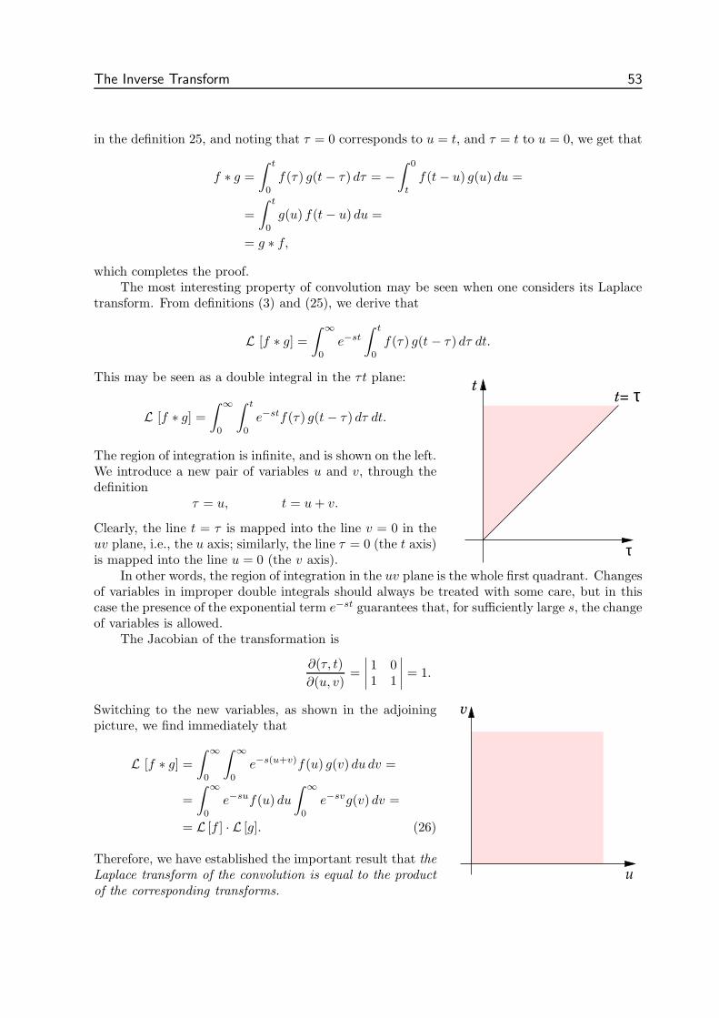
The Inverse Transform 53
in the definition 25, and noting that τ = 0 corresponds to u = t, and τ = t to u = 0, we get that
f ∗ g =
∫ t
0
f(τ) g(t − τ) dτ = −∫ 0
t
f(t − u) g(u) du =
=
∫ t
0
g(u) f(t − u) du =
= g ∗ f,
which completes the proof.The most interesting property of convolution may be seen when one considers its Laplace
transform. From definitions (3) and (25), we derive that
L [f ∗ g] =
∫ ∞
0
e−st
∫ t
0
f(τ) g(t − τ) dτ dt.
This may be seen as a double integral in the τt plane:
L [f ∗ g] =
∫ ∞
0
∫ t
0
e−stf(τ) g(t − τ) dτ dt.
The region of integration is infinite, and is shown on the left.We introduce a new pair of variables u and v, through thedefinition
τ = u, t = u + v.
Clearly, the line t = τ is mapped into the line v = 0 in theuv plane, i.e., the u axis; similarly, the line τ = 0 (the t axis)is mapped into the line u = 0 (the v axis).
τt
τ
t=
In other words, the region of integration in the uv plane is the whole first quadrant. Changesof variables in improper double integrals should always be treated with some care, but in thiscase the presence of the exponential term e−st guarantees that, for sufficiently large s, the changeof variables is allowed.
The Jacobian of the transformation is
∂(τ, t)
∂(u, v)=
∣
∣
∣
∣
1 01 1
∣
∣
∣
∣
= 1.
Switching to the new variables, as shown in the adjoiningpicture, we find immediately that
L [f ∗ g] =
∫ ∞
0
∫ ∞
0
e−s(u+v)f(u) g(v) du dv =
=
∫ ∞
0
e−suf(u) du
∫ ∞
0
e−svg(v) dv =
= L [f ] · L [g]. (26)
Therefore, we have established the important result that theLaplace transform of the convolution is equal to the product
v
u
of the corresponding transforms.
54 The Inverse Transform
Example 69 Find the Laplace transform of f(t) =∫ t
0τ√
t − τ dτ .
Solution: Note that f(t) = t ∗√
t; therefore
L [f(t)] = L [t] · L[√
t]
.
It follows immediately that
L[∫ t
0
τ√
t − τ dτ
]
= L[
t ∗√
t]
= L [t] · L[√
t]
=1
s· (1/2)!
s3/2=
√π
2s5/2.
Example 70 Find the Laplace transform of f(t) =∫ t
0(t − τ)3 cosh τ dτ .
Solution: Note that∫ t
0
(t − τ)3 cosh τ dτ = t3 ∗ cosh t;
since
L [t3] =3!
s4, L [cosh t] =
s
s2 − 1,
it follows immediately that
F (s) =3!
s4· s
s2 − 1=
6
s3(s2 − 1).
Example 71 Find the Laplace transform of f(t) =∫ t
0τ2e−4τ dτ using convolution.
Solution: The integral in this example is not a convolution product. Hence, we write
f(t) =
∫ t
0
τ2e−4τ dτ = e−4t
∫ t
0
τ2e4(t−τ) dτ = e−4t g(t),
where g(t) is indeed a convolution product:
g(t) = t2 ∗ e4t.
By (26), we obtain that
G(s) =2
s3(s − 4);
so finally, by the shift theorem (19) of section 1.10, we get:
F (s) = G(s + 4) =2
(s + 4)3s.
Obviously, this problem could also be done without using convolution:
F (s) =1
s· d2
ds2L
[
e−4t]
.
Verify that the answer is the same.
In applications one often needs to identify the original function f(t), knowing its transform F (s).Therefore, it is also useful to write (26) backwards, in the form
L−1[
F (s)G(s)]
= f ∗ g(t), (27)
as illustrated by the following examples.
The Inverse Transform 55
Example 72 Find f(t), if F (s) = 1/s5(s − 1)2.
Solution: We write F (s) = G(s)H(s), with
G(s) =1
s5,
H(s) =1
(s − 1)2.
It follows immediately thatg(t) = t4/4!,
h(t) = tet,
and hence that
f(t) = g ∗ h(t) = 124
∫ t
0
τ4(t − τ)et−τ dτ =
= 124et
∫ t
0
(tτ4 − τ5)e−τ dτ =
= 124
t4 + 13t3 + 3
2t2 + 4t + 5 + (t − 5)et.
Example 73 Find L−1 [1/(s2 + ω2)2] (again).
Solution: Write
F (s) =1
s2 + ω2;
it follows immediately that1
(s2 + ω2)2= F (s)F (s),
and also that
f(t) =sin ωt
ω.
Hence
L−1
[
1
(s2 + ω2)2
]
= f ∗ f(t) =
=
∫ t
0
sin ωτ sin ω(t − τ)
ω2dτ.
This integral may be done by means of the well-known identity
sinA sin B = 12
(
cos(A − B) − cos(A + B))
.
It follows that
L−1
[
1
(s2 + ω2)2
]
=
∫ t
0
cos ω(2τ − t) − cos ωt
2ω2dτ =
=
[
sinω(2τ − t)
4ω3
]t
0
−[
τ cos ωt
2ω2
]t
0
=
=2 sin ωt
4ω3− t cos ωt
2ω2.
After simplification, this may be seen to be identical to the second result of example 61.
56 The Inverse Transform
Example 74 Find u(t − 2) ∗ u(t − 3).
Solution: Taking the Laplace transform of this function, we find that
L[
u(t − 2) ∗ u(t − 3)]
=e−2s
s· e−3s
s=
e−5s
s2.
Therefore,
u(t − 2) ∗ u(t − 3) = L−1
[
e−5s
s2
]
= (t − 5)u(t − 5) =
0 if t < 5,t − 5 if t ≥ 5.
Method 2: From first principles.
u(t − 2) ∗ u(t − 3) =
∫ t
0
u(τ − 2)u(t − τ − 3) dτ
As an exercise, verify that the answer is the same.
Example 75 Find the convolution of t−1/2 with itself and hence calculate (−1/2)!.
Solution: We start from the basic transform of tc; see (9) in chapter 1. With c = −1/2, we getthe equation
L[
1√t
]
=(−1/2)!√
s.
Hence, by convolution, we get that
L[
1√t∗ 1√
t
]
=(−1/2)!√
s· (−1/2)!√
s=
(
(−1/2)!)2
s.
Expanding this equation, we obtain
L[
∫ t
0
dτ√τ√
t − τ
]
=(
(−1/2)!)2 L [1]
and hence (inverting the Laplace transform)
∫ t
0
dτ√τ√
t − τ=
(
(−1/2)!)2
.
The integral on the left-hand side is elementary: substituting τ = tx2, dτ = 2tx dx, we getimmediately
∫ 1
0
2 dx√1 − x2
= π =(
(−1/2)!)2
,
and finally (−1/2)! =√
π.
You might be surprised to learn that f(t) ≡ 1 is not the “unit” of convolution product; in otherwords 1∗f(t) is not in general equal to f(t). Indeed, the problem of finding a function δ(t) withthe property that δ ∗ f(t) = f(t) for every f(t) leads straight into operational calculus, whichyou’ll encounter at a later stage of your studies.
The Inverse Transform 57
Example 76 Find 1 ∗ t.
Solution: Since 1 ∗ t = t ∗ 1, we get immediately:
t ∗ 1 =
∫ t
0
τ dτ = 12 t2.
In other words, 1 ∗ t = 12 t2.
8. Additional Examples
Using the Laplace transform it is possible to calculate some definite integrals that cannot bedone by elementary calculus. Broadly speaking, all the following examples use the same trick,i.e., an interchange (done at the right time) of the order of integration. As mentioned before, arigorous justification of this step (though not difficult) is beyond the scope of these notes.
Example 77 Calculate∫ ∞0
cos tx dx/(1 + x2), where t is a positive parameter.
Solution: Define an auxiliary function a(t) as follows:
a(t) =
∫ ∞
0
cos tx
1 + x2dx.
Taking the Laplace transform of a(t), we get:
A(s) =
∫ ∞
0
e−st
[∫ ∞
0
cos tx
1 + x2dx
]
dt.
This may be seen as a double integral over the whole first quadrant of the xt plane (an improperintegral, of course). Swapping the order of integration, we get:
A(s) =
∫ ∞
0
1
1 + x2
∫ ∞
0
e−st cos tx dt dx.
The inner integral is just the Laplace transform of cos tx:
∫ ∞
0
e−st cos tx dt =s
s2 + x2.
Substituting this result into the preceding equation, we obtain:
A(s) =
∫ ∞
0
s
(1 + x2)(s2 + x2)dx.
This integral is elementary. Evaluating it (partial fractions are required), one gets
A(s) =s
s2 − 1
[
arctan x − arctan(x/s)
s
]∞
0
=
=s
s2 − 1
[
12π −
12π
s
]
=
=12π
s + 1= 1
2πL[
e−t]
.
58 The Inverse Transform
It follows∫ ∞
0
cos tx
1 + x2dx = a(t) = 1
2πe−t.
Corollary: Differentiating this equation with respect to t, we get immediately that∫ ∞
0
x sin tx
1 + x2dx = −a(t) = 1
2πe−t.
Example 78 Calculate (−1/2)! without using convolution.
Solution: Define the auxiliary function
a(t) =
∫ ∞
0
e−tu2
du. [t > 0]
Substituting tu2 = x, which yields du = t−1/2 · 12x−1/2 dx, we get
a(t) = 12 t−1/2
∫ ∞
0
x−1/2e−x dx = 12 t−1/2
(
− 12
)
!,
and hence, substituting c = − 12 into (9),
A(s) =12
[(
− 12
)
!]2
s1/2. (28)
We now calculate A(s) again, this time from first principles:
A(s) =
∫ ∞
0
e−st
[∫ ∞
0
e−tu2
du
]
dt.
Swapping the order of integration we get
A(s) =
∫ ∞
0
[∫ ∞
0
e−ste−tu2
dt
]
du.
The inner integral is a basic transform (see (4) in section 1.3):
A(s) =
∫ ∞
0
1
s + u2du.
Integrating the right-hand side we get
A(s) =
[
arctan(u/s1/2)
s1/2
]∞
0
=12π
s1/2. (29)
Comparing (28) and (29) we get12
[(
− 12
)
!]2
s1/2=
12π
s1/2.
Simplifying, it follows(
− 12
)
! =√
π.
Corollary: Substituting t = 1 in (28), we get
a(1) =
∫ ∞
0
e−u2
du = 12
√π
which by symmetry yields∫ ∞
−∞e−u2
du =√
π,
a formula of great importance in probability theory and statistics.
The Inverse Transform 59
Example 79 Calculate∫ ∞0
s−c ds/(1 + s), where 0 < c < 1.
Solution: We note that1
s + 1= L
[
e−t]
and hence∫ ∞
0
s−c
1 + sds =
∫ ∞
0
s−cL[
e−t]
ds =
=
∫ ∞
0
s−c
[∫ ∞
0
e−te−st dt
]
ds.
Swapping the order of integration, and substituting st = u, the right-hand side becomes
∫ ∞
0
e−t
[∫ ∞
0
s−ce−st ds
]
dt =
∫ ∞
0
e−t
[∫ ∞
0
u−c
t−ce−u du
t
]
dt =
=
∫ ∞
0
e−t tc−1
[∫ ∞
0
u−ce−u du
]
dt.
In terms of generalized factorials (11), this may be written
∫ ∞
0
e−ttc−1 dt · (−c)! = (c − 1)! (−c)!.
So, finally, we get∫ ∞
0
s−c
1 + sds = (c − 1)! (−c)!
Comment: If c is irrational, this integral may not be done by the methods of elementarycalculus. However, if c = m/n with integer m and n, then the substitution s = un rationalizesthe integrand.
In particular, if c = 1/2 we get
∫ ∞
0
s−1/2
1 + sds =
[
(− 12 )!
]2,
but the left-hand side (substituting s1/2 = u) becomes
2
∫ ∞
0
du
1 + u2= π.
It follows that (− 12 )! =
√π; the same result found in examples 75 and 78.
60 Tutorial Problems The Inverse Transform
PROBLEMS
Elementary Inverse Transforms
18. Find the following inverse Laplace transforms.(a) L−1 [s−5](b) L−1 [8s/(s2 + 16)](c) L−1 [12/(4 − 3s)](d) L−1 [(2s − 5)/(s2 − 9)](e) L−1 [1/s7/2]
(f) L−1 [(√
s − 1)2/s2](g) L−1 [
√π/(s + 3)5/2]
(h) L−1 [s/(s2 + 2s + 37](i) L−1 [(2s + 3)/
√
(s + 1)3](j) L−1 [(s + 1)2/(s − 1)3]
Partial Fractions
19. Use partial fractions expansion to find the inverse Laplace transform of the followingfunctions.
(a) 1/(s2 + 4s + 5)(b) s/(s + 1)2
(c) (s3 + 1)/(s2 − s)(s2 − 4)
(d) 1/s2(s2 + 1)(e) s/(s3 + 1)(f) (2s + 3)/(s3 + 4s2 + 5s)
20. Use partial fractions expansion to find the inverse Laplace transform of the followingfunctions.
(a) (2s − 1)/(s3 − s)(b) (27 − 12s)/(s + 4)(s2 + 9)(c) (s3 + 16s − 24)/(s4 + 20s2 + 64)(d) s/(s2 − 2s + 2)(s2 + 2s + 2)(e) (11s2 − 2s + 5)/(s− 2)(s + 1)(2s− 1)
(f) 2(7s − 31)/(s3 + 3s2 − 25s + 21)(g) 27s/(s + 1)(s − 2)3
(h) (s + 1)/(s2 + 2s + 2)2
(i) (s2 + 1)/s(s2 + 2)(s2 + 3)(j) (5s2 − 18s + 15)/(s − 1)(s − 2)3
Shifting
21. Find f(t), if F (s) is defined as follows.
(a) F (s) =e−3s
(s + 1)2
(b) F (s) =e−s sinh s
s
(c) F (s) =e−s/3
s(s2 + 1)
(d) F (s) =2(1 − e−3s)
s3− 3(1 + e−3s)
s2
22. Find:
(a) L−1
[
1 − e−πs + e−2πs
s2 + 1
]
(b) L−1
[
(
1 − e−πs
s
)2]
Dirty Tricks
23. Find the following inverse Laplace transforms. Read ex. 67 before doing question (h).
(a) L−1
[
2
s(s4 − 1)
]
(b) L−1
[
lns + 3
s + 1
]
(c) L−1
[
ln
√s2 + 1
s + 4
]
(d) L−1
[
1
2sln
s2 + 49
s2 + 25
]
(e) L−1
[
lns4
s4 − 1
]
(f) L−1
[
lns2 + 4s + 13
s2 + 4s + 5
]
(g) L−1[
arccot s]
(h) L−1[
s arccot s − 1]
The Inverse Transform Tutorial Problems 61
Convolution
24. Find (1 ∗ 1) ∗ sin t and 1 ∗ (1 ∗ sin t), and verify that you get the same answer.
25. Find: (a) et ∗ e−t, (b) t ∗ u(t − 8), (c) t2 ∗ u(t − 5).
26. Show that e−t2 ∗ et2 = (sinh t2)/t.
27. Use the convolution theorem to calculate the following Laplace transforms.
(a) L[
∫ t
0(t − τ)4 sin 3τ dτ
]
(b) L[
∫ t
0(t − τ)137e−4τ dτ
]
28. Show that
(a) cos t ∗ cos t + sin t ∗ sin t = sin t,
(b) cosh t ∗ cosh t − sinh t ∗ sinh t = sinh t.
29. Use the convolution theorem to calculate the following inverse Laplace transforms.(a) L−1
[
1/
(s + 1)(s2 + 2s + 50)]
(b) L−1[
1/
(s − 1)3(s + 1)]
Calculation of Integrals
30. Show that
∫ ∞
0
e−2t sin2 t
tdt = 1
4ln 2.
31. Show that
∫ ∞
0
e−3t − e−6t
tdt = ln 2.
32. Show that
∫ ∞
0
cos 2t − cos 14t
tdt = ln 7.
33. Show that
∫ ∞
0
x4e−x2
dx = 3√
π/8.
ANSWERS
18 (a) t4/24
(b) 8 cos 4t
(c) −4e4t/3
(d) 2 cosh 3t − 53 sinh 3t
(e) 8t5/2/15√
π
(f) 1 + t − 4√
t/√
π
(g) 43
t3/2e−3t
(h) e−t(cos 6t − 16 sin 6t)
(i) 2e−t(1 + t)/√
πt
(j) et(1 + 4t + 2t2)
19 (a) e−2t sin t
(b) (1 − t) e−t
(c) 14− 2
3et + 9
8e2t + 7
24e−2t
(d) t − sin t
(e) 13et/2
(
cos√
3t/2 +√
3 sin√
3t/2)
− 13e−t
(f) 15
(
3 + e−2t(4 sin t − 3 cos t))
20 (a) 1 − 32e−t + 1
2et
(b) 3e−4t − 3 cos 3t
(c) 12 sin 4t + cos 2t − sin 2t
(d) 12 sin t sinh t
(e) 5e2t − 32et/2 + 2e−t
(f) 3et − e3t − 2e−7t
(g) e−t + (9t2 + 3t − 1)e2t
(h) 12 te−t sin t
(i) 16 + 1
2 cos√
2t − 23 cos
√3t
(j) −2et + (2 + 3t − 12t2)e2t
21 (a) f(t) = (t − 3)e−(t−3)u(t − 3) =
0 if t < 3(t − 3)e−(t−3) if t > 3
62 Tutorial Problems The Inverse Transform
(b) f(t) = 12
(
u(t) − u(t − 2))
=
12 if 0 < t < 20 everywhere else.
(c) f(t) =
0 if t < 1/31 − cos(t − 1
3) if t > 1/3
(d) f(t) =
t(t − 3) if 0 < t < 30 everywhere else; see example 33.
22 (a) f(t) =
0 if t is negative,sin t if 0 < t < π,sin 2t if π < t < 2π,sin 3t if t is greater than 2π.
(b) f(t) =
t if 0 < t < π,2π − t if π < t < 2π,0 everywhere else.
23 (a) cosh t + cos t − 2
(b)e−t − e−3t
t
(c)e−4t − cos t
t
(d)
∫ t
0
cos 5τ − cos 7τ
τdτ
(e)2 cosh t + 2cos t − 4
t
(f)2e−2t(cos t − cos 3t)
t
(g)sin t
t
(h)cos t
t− sin t
t2.
Note: The integral in 23(d) cannot be done by elementary calculus.
24 t − sin t.
25 (a) sinh t, (b) 12
(t − 8)2 · u(t − 8), (c) 13
(t − 5)3 · u(t − 5).
26 Hint:∫ t
0e−τ2
e(t−τ)2 dτ = ?
27 (a) 72/s5(s2 + 9), (b) 137!/s138(s + 4).
29 (a) e−t(1 − cos 7t)/49, (b)(
12t2 − 1
2t + 1
4
)
et − 14e−t.
33 Hint: Substitute x2 = u. Recall the definition of generalized factorial.
Linear Differential Equations 63
Chapter Three
LINEAR DIFFERENTIAL EQUATIONS
1. Linearity
An expression of the formc2 x + c1 x + c0 x = f, (30)
where x is an unknown function of one variable, whereas c2, c1, c0 and f are given functions, isa linear differential equation of 2nd order. If the term c2x is missing, the equation is said to beof 1st order; linear differential equations of order 3, 4 and up, are defined in the obvious way.
In this chapter we’ll continue to use t as the independent variable, as we did in the precedingchapters.†
Example 80 The equation t2x− (t2 +2t) x+(t+2)x = t4 is 2nd-order linear. We find thatc2 = t2, c1 = −(t2 + 2t), c0 = t + 2 and f = t4.
The quantities c2, c1 and c0 are also called the coefficients of the equation. The special casewhere the coefficients are all constant is very important in applications, and we’ll study it ingreater detail.
Example 81 The equation 5x−8x+3x = sin t is a linear equation with constant coefficients;we find that c2 = 5, c1 = −8, c0 = 3 and f(t) = sin t.
Before we proceed, we shall quickly review the concept linearity in general.Linear differential equations are members of the larger family of linear equations. Linear
equations have certain important common features, which connect directly to the methods oflinear algebra that you have already studied in other courses. Let’s take a quick look at someof these unifying properties.
Definition: An equation is called linear if it may be expressed in the form
O x = f,
where x is an unknown quantity, f is given, and O is an operator having the property
O (s1x1 + s2x2) = s1O x1 + s2O x2
for all operands x1, x2 and scalars s1, s2.
† Most books use x as independent variable, and y(x) as dependent.
64 Linear Differential Equations
This definition is extremely general. For example:
• If the unknown quantity x is a column vector, and O is a matrix, then we have a system oflinear equations of the kind you met in first-year linear algebra. The systems of equationsyou saw in high school also fall in this group.
• If x is a function of t, and O a linear combination of derivatives, then we have a linearordinary differential equation [ODE for short] like (30), or also like examples 80–81.
• If x is a function of t, and O x is defined through an integral like
O x(t) =
∫ b
a
x(τ)
t2 + τ2dτ
then we have a linear integral equation.• If x is a column of functions of t, and O a matrix where every row is a linear combination
of derivatives, we have a system of coupled differential equations. We shall see examplesfurther on (in section 3.9).
• If x is the angular velocity of a rigid body, f is the torque on the body, and O is itsinertia tensor, then we get Euler’s equations for rigid-body motion, which are particularlyimportant for mechanical engineers.
• If x is a function of y and z, and O is a linear combination of partial derivatives, like
5xyy + 3xzz = f(y, z),
then we have a linear partial differential equation [PDE for short].
The list of examples is virtually endless; among the ones shown above, some are already toodifficult for this course.
Note that the symbol x represents a different mathematical “object” in each of these exam-ples. As a rule, the set of all possible x that may go under the operation O, has the structure ofa vector space. This space could be the familiar R
3 of physics, or Rn, like in your linear algebra
courses—or even more abstract, as you’ll see later in the course of your studies. However, thestructure of the equation is the same in all cases.
Several definitions are applicable to all these examples; they also have certain commonproperties. For example:
• If the right-hand side is zero the equation is called homogeneous.• Solutions of an homogeneous linear equation form a vector subspace (i.e., they are closed
under addition and scalar multiplication), called the kernel or null-space of O.• If there is a number λ such that the equation O x = λx has non-trivial solutions, then λ is
called an eigenvalue of O.• Every non-homogeneous linear equation may be associated with a corresponding homoge-
neous equation, by replacing the right-hand side with zero.• If x1 and x2 are solutions of the same non-homogeneous linear equation, their difference
x1 − x2 is a solution of the corresponding homogeneous equation.
A quick revisitation of linear algebra will help make these ideas clear.
Example 82 Consider the system
[
5 17 33 10 2
]
x1
x2
x3
=
[
−30
]
. (31)
Linear Differential Equations 65
Simple row-reduction yields:x1 = 30 − 4x3
x2 = −9 + x3,
hence, writing x3 = t, we get:
x1
x2
x3
=
30−90
+ t
−411
.
This equation shows that the system has an infinity of solutions, parametrized by t. One suchsolution (corresponding to t = 0) is represented by [ 30 −9 0 ]T , the first vector on theright-hand side. Other solutions are obtained by fixing t to different values. For example
x1
x2
x3
=
26−81
, or
−609
, or
−10110
, . . .
are also solutions. Note that the difference between any two of them is a scalar multiple of[−4 1 1 ]
T, which in turn is a solution of the corresponding homogeneous system:
[
5 17 33 10 2
]
h1
h2
h3
=
[
00
]
, (32)
h1
h2
h3
= t
−411
.
We see that the null-space of the matrix for the system (32) is one-dimensional, and its basis
consists of the single vector [−4 1 1 ]T.
Observe also that if we complement the system (31) with one auxiliary condition of theform, say,
x1 = 0,
then the resulting problem has a unique solution, corresponding to t = 7.5:
x1
x2
x3
=
30−90
+ 7.5
−411
=
0−1.57.5
.
Although this example is elementary, it has the same structure of the more advanced problems indifferential equations and systems of equations that we are about to study. Note, in particular,the difference between the general solution, which contains the free parameter t, and a particularsolution that meets an additional requirement.
It is not surprising that differential equations with constant coefficients and systems oflinear algebraic equations like (31), should be so similar. The link between them is representedprecisely by the Laplace transform, which transforms linear differential equations into “plain”linear equations.
66 Linear Differential Equations
2. Linear ODEs: Preliminary Comments
As a rule, a differential equation is regarded as “solved” if it’s possible to write down the solutionin terms of integrals, even if such integrals cannot be done by elementary calculus.
Example 83 The function x = t∫
(sin t/t2) dt is a solution (not the only one) of the equationtx − x = sin t, as you may check using the product rule. However,
∫
(sin t/t2) dt may not bedone by the rule of elementary calculus.
Broadly speaking, the problem of solving ODEs tends to get more and more complicated as theorder of the equation† increases.
For example, we’ll see that linear equations of order 1 may always be solved, in the sensegiven above; on the other hand, there is no general, “all-purpose” method for solving arbitrary2nd-order linear ODEs like (30), or ODEs of higher order. So, in moving from first-order tosecond-order, we already encounter a major complication.
However, for linear ODEs with constant coefficients (recall, they are the equations where thecoefficients c0, c1, c2 etc are all constant) it is always possible to solve the equation, regardlessof its order. One way to do that is by the Laplace transform.
Example 84 Solve the differential equation x + 7x + 10x = 0, given that x(0+) = 2 andx(0+) = −1.
Solution: The coefficients are 1, 7 and 10. Applying the Laplace transform, we get:
L [x] = X, L [x] = sX − 2, L [x] = s2X − 2s + 1.
Substituting these expressions into the equation, we obtain an equation for X:
s2X − 2s + 1 + 7(sX − 2) + 10X = 0,
which yields
X =2s + 13
s2 + 7s + 10=
2s + 13
(s + 2)(s + 5)=
3
s + 2− 1
s + 5.
Finally, applying the inverse transform, we get that
x = 3e−2t − e−5t.
This is the solution we seek and, by Lerch’s theorem, it’s unique.
Example 85 Solve the differential equation y + 9y = sin 2t, given that y(0+) = 7 andy(0+) = −3.
Solution: The coefficients are 1, 0 and 9. Applying the Laplace transform to both sides of theequation, we get that L [y] = Y , L [y] = s2Y − 7s + 3 and L [sin 2t] = 2/(s2 + 4). Hence,
s2Y − 7s + 3 + 9Y =2
s2 + 4
Y =2
(s2 + 4)(s2 + 9)+
7s − 3
s2 + 9.
† This is, by definition, the order of the highest derivative of the solution.
Linear Differential Equations 67
Simple manipulations yield
2
(s2 + 4)(s2 + 9)=
2/5
s2 + 4−
2/5
s2 + 9.
Hence,
Y =2/5
s2 + 4−
17/5
s2 + 9+
7s
s2 + 9.
Finally, inverting the transform, we find that our solution is
y = 15
sin 2t − 1715
sin 3t + 7cos 3t.
These examples illustrate some important ideas.
• First of all, the equation in example 84 is homogeneous while the one in example 85 isnon-homogeneous, but the Laplace transform deals with them in essentially the same way.
• Another point to be noted is that both examples are second-order: we’ll see that for equa-tions with constant coefficients, problems of third and higher order may be tackled in thesame way as second-order problems. Hence, most of our examples will be second-orderproblems.
• Both examples came with exactly two additional bits of information, one about the unknownand one about its first derivative. Technically, these are called initial conditions, becausethey prescribe the value of two unknown functions at the same t (which was t = 0 in bothexamples). So, we have seen how a second-order linear ODE with constant coefficients withtwo initial conditions may be solved completely and uniquely. If you followed so far, you’llprobably guess that three initial conditions would be needed for a third-order equation, fourinitial conditions for a fourth-order one, and so on; and your guess would be correct.
• An important property of linear ODEs is that, for an equation of order n, there is alwaysone (and only one) solution satisfying n initial conditions, on the unknown and its firstn−1 derivatives, set at the same time t0. Mathematicians call this result an “existence anduniqueness” theorem. Linear initial-value problems have several nice features, and this isone of them. From an engineer’s point of view, though, the uniqueness bit is probably themore useful one. In simple words, it means that if we have been able, somehow, to find asolution, then we know we found the solution, because it is the only one: we have to lookno further.
• In more advanced engineering problems, you’ll encounter problems where requirementsmust be made at different t’s, for example at t = 0 and t = 4. These are called boundaryconditions, but we’ll not discuss them here.
• Finally, in some applications one may need to solve a linear differential equation withoutspecifying any initial conditions. This may be done by treating the initial data as “free”parameters. The solution obtained in this way is the general solution, as opposed to aparticular solution corresponding to a set of initial conditions.
It is easy to show that the solutions of a linear homogeneous ODE form a vector space (afterall, they are just the kernel of a linear operator). So, finding the general solution of a linearhomogeneous ODE means finding a basis for such a space.
Definition: The set of all solutions of a homogeneous linear differential equation is called thesolution space of the equation.
68 Linear Differential Equations
It is also possible to prove that the dimension of the solution space is always equal to the orderof the equation: a third-order linear homogeneous ODE has always a three-dimensional solutionspace, a fourth-order has a four-dimensional solution space, and so on.
But remember that this principle applies only to homogeneous linear ODEs; the solutionset of a non-homogeneous linear ODE is never a vector space.
To make this point clear, let us go back to examples 84 and 85, which are both second-orderproblems.
Example 86 Check that any linear combination of e−2t and e−5t is a solution of the equationx + 7x + 10x = 0.
Solution: Indeed, if we writex = Ae−2t + Be−5t
for arbitrary A and B, then we see that
x = −2Ae−2t − 5Be−5t,
x = 4Ae−2t + 25Be−5t.
Substituting these expressions into the equation, we get:
4Ae−2t + 25Be−5t + 7(−2Ae−2t − 5Be−5t) + 10(Ae−2t + Be−5t) = 0,
and finally, for any value of A and B, we get 0 = 0, which completes the check.
On ther other hand, if the ODE is non-homogeneous, the check fails.
Example 87 Go back to example 85, where the equation was y + 9y = sin 2t. Take twosolutions: for instance y1 = sin 3t+ 1
5 sin 2t and y2 = cos 3t+ 15 sin 2t are solutions. First of all,
we verify that y1 and y2 are indeed solutions. We have:
y1 = −9 sin 3t − 45 sin 2t y2 = −9 cos 3t − 4
5 sin 2t.
Substituting these expressions into the equation, we obtain:
y1 + 9y1 = (−9 + 9) sin 3t + (− 45 + 9
5 ) sin 2t =
= sin 2t.
y2 + 9y2 = (−9 + 9) cos 3t + (− 45 + 9
5 ) sin 2t =
= sin 2t.
So, both y1 and y2 yield the identity sin 2t = sin 2t, which means they are solutions. However,if we substitute a simple linear combination such as
y = 7y1 − 3y2
into the equation, we get (7− 3) sin 2t = sin 2t, i.e., 4 = 1, which is absurd. This shows that ourlinear combination of solutions is not a solution.
3. Linear Homogeneous ODEs with Constant Coefficients
The general solution of a homogeneous equation with constant coefficients may be always foundfollowing a few simple rules. We’ll first look at some numeric examples, after which it will beeasy to see the general procedure.
Linear Differential Equations 69
Example 88 Find the general solution of the equation x − 5x − 14x = 0.
Solution: As the initial values of x and x are not specified, we treat them as parameters. We set
x(0+) = a = free, x(0+) = b = free;
it follows, by the Laplace transform:
s2X − sa − b − 5X + 5a − 14X = 0.
Solving for X, we get:
X =sa + b − 5a
s2 − 5s − 14=
sa + b − 5a
(s − 7)(s + 2).
The right-hand side may be expanded by Heaviside’s method:
X(s) =19(2a + b)
s − 7+
19(7a − b)
s + 2.
However, we don’t need to keep X in such a complicated form. Since a and b are free andindependent parameters, we introduce two new parameters
A = 19(2a + b) B = 1
9(7a − b) :
clearly, A and B are also free and independent. Therefore, we may write
X =A
s − 7+
B
s + 2,
where A and B are free, and finally
x(t) = Ae7t + Be−2t;
we may leave the general solution in this form.
Example 89 Find the general solution of the equation x − 4x + 4x = 0.
Solution: Transforming the equation, we get that
s2X − sa− b − 4(
sX − a)
+ 4X = 0,
where a = x(0+) and b = x(0+). It follows that
(s2 − 4s + 4)X = sa + b + 4a.
Reasoning like in example 88, we write
X =sa + b + 4a
s2 − 4s + 4=
sa + b + 4a
(s − 2)2=
A
s − 2+
B
(s − 2)2,
where A and B are free parameters linked to the initial data on x and x. Inverting the Laplacetransform, we get
x(t) = Ae2t + Bte2t,
and this is the general solution.
70 Linear Differential Equations
THE CHARACTERISTIC EQUATION
Having seen two examples, let’s try to understand how the method works from a higher pointof view. Consider a linear homogeneous 2nd-order ODE with constant coefficients, like
c2x + c1x + c0x = 0
where c2, c1 and c0 are constants. We take the Laplace transform of this equation, treating theinitial data as “free” parameters. Eventually, we get for X an expression like
X =(A first degree polynomial in s)
c2s2 + c1s + c0.
The denominator D(s) on the right-hand side is called the characteristic polynomial of theequation, and it’s obtained by replacing x with s2 and x with s in the original equation.
If the characteristic equation
c2s2 + c1s + c0 = 0
has two roots s = r1 and s = r2, then the characteristic polynomial D(s) may be factored as
c2s2 + c1s + c0 = c2(s − r1)(s − r2).
This, in turn, leads to a partial fractions expansion of the form
X =A
s − r1+
B
s − r2,
where A and B are “free”, and finally to the general solution
x = Ae−r1t + Be−r2t.
If, on the other hand, the characteristic equation has only one root s = r, then the charac-teristic polynomial may be factored as
c2s2 + c1s + c0 = c2(s − r)2,
which leads to a partial fractions expansion of the form
X =A
s − r+
B
(s − r)2
and finally to the general solution
x = Ae−rt + Bte−rt.
Conclusion: In practice one may bypass the Laplace transform, since the general solutiondepends only on the characteristic roots (or root): once they have been determined, the solutionmay be written down immediately.
The extension of this procedure to higher order equations of the form
cnx(n) + . . . + c2x + c1x + c0x = 0. (33)
is obvious, so let’s see it quickly. By taking the Laplace transform of (33), one arrives at asolution of the form
X(s) =(A polynomial of degree n − 1 in s)
D(s), (34)
where D(s) is the characteristic polynomial—obtained by replacing x(n) with sn, x(n−1) withsn−1, and so on and so forth, in equation (33)—and the numerator depends on n free parameters,one for each initial condition.
Then, D(s) is broken into factors: this step always requires finding the roots of the equationD(s) = 0, which is the characteristic equation for the given differential equation.
Linear Differential Equations 71
Definition: The roots of the characteristic equation are called characteristic roots.
If the linear factors of D(s) are all distinct we say that the roots are simple. For instance, inexample 88 we saw D(s) could be written as the product of (s + 2) and (s − 7) : so −2 and 7are simple roots. But in example 89, we saw D(s) could only be written as (s− 2)(s− 2), so the(only) root s = 2 was not simple.
Definition: If a polynomial D(s) may be written as a product like D(s) = (s−r)m Q(s), whereQ(s) is another polynomial and Q(r) 6= 0, we say that r is a root of D(s) with multiplicity m.Roots with multiplicity 1, 2 and 3 are often called simple, double and triple, respectively.
Example 90 The root s = 2 in example 89 is double. The characteristic polynomial isD(s) = s2 − 4s + 4 and may be factored as D(s) = (s − 2)2.
Example 91 The polynomial D(s) = s7 + 2s5 + s3 may be factored as D(s) = s3(s2 + 1)2 =s3(s − i)2(s + i)2. Hence, s = 0 is a triple root and s = i, −i are double complex roots.
Example 92 Using the free computer package maxima, one may quickly see that for thepolynomial D(s) = s8 − 11s7 + 33s6 − 5s5 − 50s4 one has D(s) = s4(s − 2)(s − 5)2(s + 1).Therefore, 2 and −1 are simple roots; 5 is a double root; 0 is a root with multiplicity 4.
Note that in the last example the multiplicities add up to n = 8, which is also the degree of thecharacteristic equation. This is no coincidence: indeed, it is easy to prove† that a polynomial ofdegree n has either n simple roots in the complex field or, if some roots are multiple, the sumof all the multiplicities is n.
If all the roots of the characteristic polynomial are simple, then, continuing from (34) weget an expansion of the form
X(s) =A
s − r1+
B
s − r2+
C
s − r3+
D
s − r4+ · · ·
and the number of terms on the right-hand side is equal to the order of the equation. Invertingthe Laplace transform we get
x(t) = Aer1t + Ber2t + Cer3t + Der4t + · · · ;
the coefficients A, B, C, D, . . . are free parameters in the general solution.
SIMPLE ROOTS: EXAMPLES
Example 93 Find the general solution of the equation x(4) − 10x + 9x = 0.
Solution: The characteristic polynomial is
D(s) = s4 − 10s2 + 9 = (s2 − 9)(s2 − 1).
† It is really a corollary of the fundamental theorem of algebra which, however, is buried deepinto the theory of complex variables.
72 Linear Differential Equations
Its roots are r1 = −3, r2 = 3, r3 = −1, r4 = 1. Each root is simple; note that there are fourroots, and the order of the equation is four. Hence, the general solution may be written
x(t) = Ae−3t + Be3t + Ce−t + Det.
Comment: the general solution may also be written
x(t) = M cosh 3t + N sinh 3t + P cosh t + Q sinh t;
convince yourself of this. We found here two equally good bases for the solution space. Eachbasis has, of course, four elements.
Complex exponentials (if any) may be converted to sines/cosines through Euler’s formula.
Example 94 Find the general solution of the equation 2x − 6x + 5x = 0.
Solution: The characteristic polynomial is
D(s) = 2s2 − 6s + 5.
Its roots are
s =3 ±
√9 − 10
2=
3 ± i
2.
Therefore, the general solution may be written as
x(t) = c1e(3+i)t/2 + c2e
(3−i)t/2 = e3t/2(c1eit/2 + c2e
−it/2).
Applying Euler’s formula, this becomes
x(t) = e3t/2(c1 cos 12 t + ic1 sin 1
2 t + c2 cos 12 t − ic2 sin 1
2 t) =
= e3t/2(A cos 12t + B sin 1
2t),
where A = c1 + c2, B = i(c1 − c2). Note that the first form of the general solution requirescomplex arithmetic, the second one does not.
Example 95 Find the general solution of 3 ˙x + x − 75x − 25x = 0.
Solution: The characteristic polynomial is
D(s) = 3s3 + s2 − 75s − 25 = s2(3s + 1) − 25(3s + 1).
Therefore, the characteristic equation may be factorized as
(3s + 1)(s2 − 25) = 0 =⇒
3s + 1 = 0,s2 − 25 = 0.
The characteristic roots are s = −1/3, s = 5 and s = −5. So, finally, the general solution is
x = Ae−t/3 + B e5t + C e−5t.
An alternative solution is x = Ae−t/3 + M cosh 5t + N sinh 5t (convince yourself of this).
Linear Differential Equations 73
Example 96 Find the general solution of the equation x(6) − 9x(3) + 8x = 0.
Solution: The characteristic equation of this 6th-order equation is
s6 − 9s3 + 8 = 0;
substituting s3 = u this becomes u2 − 9u + 8 = 0, which factorizes as (u − 1)(u − 8) = 0.Therefore the characteristic roots are given by the equations
s3 − 1 = 0 and s3 − 8 = 0.
Simple manipulations yield
s =
1(
− 1 + i√
3)
/2(
− 1 − i√
3)
/2and s =
2−1 + i
√3
−1 − i√
3
Therefore, the general solution in real form is
x = Aet + e−t/2(
B cos√
3t/2 + C sin√
3t/2)
+ Me2t + e−t(
N cos√
3t + P sin√
3t)
.
MULTIPLE ROOTS: EXAMPLES
If the characteristic polynomial has a double root r, and some other roots, we proceed like inexample 89: going back to (34), we get
X(s) =A
s − r+
B
(s − r)2+ (n − 2 terms that do not depend on r),
where A and B are “free”. The general solution will then have the form
x(t) = Aert + Btert + (n − 2 exponentials that do not depend on r).
Similarly, if the characteristic polynomial has a triple root r, and perhaps other roots, continuingfrom (34), we get
X(s) =A
s − r+
B
(s − r)2+
C
(s − r)3+ (n − 3 terms that do not depend on r),
and the general solution will have the form
x(t) = Aert + Btert + 12Ct2ert + (n − 3 exponentials that do not depend on r).
Note, however, that the factor 12 attached to C may be removed without loss of generality,
because C is free, anyway.The pattern is now clear: a quadruple characteristic root r would contribute a combination
of solutions of the form Aert + Btert + Ct2ert + Dt3ert to the general solution, and so on. Acharacteristic root of multiplicity m would contribute a linear combination of m terms. Again,complex exponentials (if any) may be handled by means of Euler’s formula.
74 Linear Differential Equations
Example 97 Find the general solution of the equation x(4) − 6x + 8x − 3x = 0.
Solution: The characteristic polynomial is
D(s) = s4 − 6s2 + 8s − 3
By inspection, D(1) = 0; hence s = 1 is a root. By long division,
s4 − 6s2 + 8s − 3
s − 1= s3 + s2 − 5s + 3.
By inspection, the right-hand side is zero if s = 1: hence, s = 1 is at least a double root. Againby long division,
s3 + s2 − 5s + 3
s − 1= s2 + 2s − 3.
Now, the right-hand side may be factored as (s − 1)(s + 3). So, putting everything together:
D(s) = s4 − 6s2 + 8s − 3 =
= (s − 1)(s3 + s2 − 5s + 3) =
= (s − 1)2(s2 + 2s − 3) =
= (s − 1)3(s + 3).
The last line shows that D(s) has only two roots, namely s = 1 (triple), and s = −3 (simple).Therefore, the general solution is
x(t) =(
A + Bt + Ct2)
et + Me−3t,
where A, B, C and M are free.
Example 98 Find the general solution of the equation y(4) + 18y + 81y = 0.
Solution: The characteristic polynomial is
D(s) = s4 + 18s2 + 81 = (s2 + 9)2.
We see that the roots are i3 and −i3, each with multiplicity 2. Hence the general solution maybe written as
y(t) =(
A1 + A2t)
ei3t +(
B1 + B2t)
e−i3t,
but also (through a suitable new set of parameters) as
y(t) =(
M + Nt)
cos 3t +(
P + Qt)
sin 3t.
Linear Differential Equations 75
4. The Non-Homogeneous Equation
A non-homogeneous linear ODE of order n with constant coefficients has the form
cnx(n) + · · · + c2x + c1x + c0x = f(t). (35)
Suppose x(t) and y(t) are two solutions of (35), leaving the initial conditions un-specified. Exceptfor the requirement that they be distinct, x and y are completely arbitrary. This, in other words,means that
cnx(n) + · · · + c2x + c1x + c0x = f(t),
cny(n) + · · · + c2y + c1y + c0y = f(t)
Subtracting one equation from the other, we get that
cn
(
x(n) − y(n))
+ · · · + c2
(
x − y)
+ c1
(
x − y)
+ c0
(
x − y)
= 0.
This shows that
zdef= x − y
is a solution of the associate homogeneous equation:
cnz(n) + · · · + c2z + c1z + c0z = 0.
So, if we have determined just one solution y of (35), regardless of the initial conditions, wemay generate any other solution x by simply adding to y the general solution of the associatehomogeneous equation. In a sense, solving the associate homogeneous equation is the heart ofthe problem. Having solved that, it does not matter which “special” solution y we add, nor howwe manage to find it.†
For equations with constant coefficients, the Laplace transform is often a good way to finda special solution. As for the initial conditions, they are free, so we may set them all to zero,which seems to be the simplest choice.
Example 99 Find the general solution of x − 2x − 3x = sinh t.
Solution: Begin with the associate homogeneous equation, which has characteristic polynomialD(s) = s2 − 2s− 3. Equating this to zero yields the characteristic roots s = −1 and s = 3, bothsimple. Hence the general solution of the associate homogeneous equation is
z = Ae−t + Be3t.
A particular solution y of the “full”, non-homogeneous equation, satisfying the initial conditionsy(0+) = y(0+) = 0, is then found by the Laplace transform: this gives
(s2 − 2s − 3)Y =1
s2 − 1
(s − 3)(s + 1)Y =1
(s − 1)(s + 1).
† This statement remains true for all linear equations, but a general discussion of linearequations with variable coefficients (beyond first-order) would be too advanced for these notes.
76 Linear Differential Equations
Solving for Y we find
Y =1
(s − 3)(s − 1)(s + 1)2=
1/32
s − 3−
1/8
s − 1+
3/32
s + 1+
1/8
(s + 1)2. (36)
Inverting the transform, it follows:
y = 132e3t − 1
8et + 332e−t + 1
8 te−t.
Finally, the general solution x = y + z may be written:
x = 132
e3t − 18et + 3
32e−t + 1
8te−t + Ae3t + Be−t,
= (A + 132 )e3t + (B − 1
8 )e−t − 18et + 1
8 te−t.
Recall, however, that A and B are free parameters; hence, if we define M = A + 132
andN = B − 1
8, we may write simply that
x = Me3t + Ne−t − 18et + 1
8 te−t,
where M and N are free. With hindsight, we realize that only two coefficients in the partialfractions expansion (36) were needed: as a rule, whenever a number is added to, or multipliedby, an undetermined parameter, it may be dropped without loss of generality.
Example 100 Find the general solution of ˙x − 3x + 3x − x = t2et.
Solution: The associate homogeneous equation has the particularly simple characteristic equation
D(s) = s3 − 3s2 + 3s − 1 = 0,
which becomes(s − 1)3 = 0,
showing immediately that its general solution z is a linear combination of et, t et and t2 et.Proceeding like in the preceding example, we take the Laplace transform of the non-
homogeneous equation setting all initial conditions to zero. Noting that
L[
t2et]
=2!
(s − 1)3
we get that
(s3 − 3s2 + 3s − 1)Y (s) =2!
(s − 1)3.
Solving for Y we find that
Y (s) =2!
(s − 1)6;
inverting the transform we obtain
y(t) =2! t5 et
5!=
t5 et
60.
The general solution of the non-homogeneous equation is
x = y + z =(
A + Bt + Ct2 + 160 t5
)
et.
Example 101 Find the general solution of x(4) − 5x − 36x = cos 2t.
Solution: The associate characteristic equation is s4 − 5s2 − 36 = 0, which factors immediately
Linear Differential Equations 77
as (s2 − 9)(s2 + 4) = 0. Hence, the characteristic roots are ±3 and ±i2, all simple. The generalsolution of the associate homogeneous equation may be written
z = A cos 2t + B sin 2t + Ce3t + De−3t,
z = A cos 2t + B sin 2t + M cosh 3t + N sinh 3tbut also
(take your choice). To find a particular solution y of the non-homogeneous equation, we set theinitial conditions to zero. By the Laplace transform, we get that
(s4 − 5s2 − 36)Y =s
s2 + 4,
and hence thatY =
s
(s2 − 9)(s2 + 4)2.
Expanding in partial fractions, we get:
Y =s/169
s2 − 9− s/169
s2 + 4− s/13
(s2 + 4)2.
The last term on the right-hand side leads us back to example 61:
s/13
(s2 + 4)2= − 1
52
d
ds
[
2
s2 + 4
]
Therefore, inverting the Laplace transform, we get:
y = 1169 cosh 3t − 1
169 cos 2t − 152 t sin 2t.
Finally, the general solution may be written
x = y + z = A cos 2t + B sin 2t + M cosh 3t + N sinh 3t − 152
t sin 2t.
Note that, since A and B are free, it is not wrong to drop the terms 1169 cosh 3t and − 1
169 cos 2tfrom the general solution (same argument as in example 99).
Example 102 Find the general solution of the equation x− 2x = u(t)− u(t− 8), where u(t)is Heaviside’s step function.
Solution: The characteristic polynomial of the associated homogeneous equation is D(s) = s2−2,with roots s = ±
√2. Hence its solution may be written
z = Ae√
2t + B e−√
2t or also z = M cosh√
2t + N sinh√
2t
(the two forms are equivalent). To find a particular solution, we set all initial conditions to zero.By the Laplace transform, we get:
(s2 − 2)Y =1 − e−8s
s.
78 Linear Differential Equations
Solving for Y , we find:
Y =1 − e−8s
s(s2 − 2).
By Heaviside’s method, we obtain that
1
s(s2 − 2)=
12 s
s2 − 2−
12
s=
= L[
cosh√
2t − 1
2
]
= L[
sinh2 t/√
2]
.
Therefore,
Y =
[ 12 s
s2 − 2−
12
s
]
·(
1 − e−8s)
,
and hence,y = sinh2 t/
√2 · u(t) − sinh2(t − 8)/
√2 · u(t − 8).
Finally, x = Ae√
2t + B e−√
2t + sinh2 t/√
2 · u(t) − sinh2(t − 8)/√
2 · u(t − 8) is the generalsolution.
INITIAL VALUE PROBLEMS
If the values at t = 0 of the unknown function are set, then one seeks a particular solutionthat fits the given conditions, rather than the general solution. For equations with constantcoefficients, in that case, probably the best option is to use the Laplace transform right fromthe start. The distinction between homogeneous and non-homogeneous equations then becomesun-necessary.
Example 103 Solve the equation y + 9y = sin 2t, given that y(0+) = 0 and y(0+) = 1.
Solution: Taking the Laplace transform of both sides of the equation, we get:
s2Y − 1 + 9Y =2
s2 + 4,
Y =1
s2 + 9+
2
(s2 + 9)(s2 + 4).
A straightforward partial fractions expansion yields
2
(s2 + 9)(s2 + 4)=
2/5
s2 + 4−
2/5
s2 + 9.
Hence,
Y =2/5
s2 + 4+
3/5
s2 + 9.
Finally,y = 1
5 sin 2t + 15 sin 3t
is the particular solution fitting the given initial values.
Linear Differential Equations 79
Example 104 Solve the equation f − 4f = t, given that f(0+) = 0 and f(0+) = 1.
Solution: Taking the Laplace transform of both sides of the equation, we get:
s2F − s · 0 − 1 − 4F =1
s2.
Solving for F yields
F =s2 + 1
s2(s2 − 4).
The right-hand side may be simplified observing the identity
x + 1
x(x − 4)=
54
x − 4−
14
x.
Therefore,
F =s2 + 1
s2(s2 − 4)=
54
s2 − 4−
14
s2=
= L[
58 sinh 2t − 1
4 t]
.
Therefore, the particular solution is f(t) = 58 sinh 2t − 1
4 t.
Example 105 Solve x − 6x + 9x = 0, with the initial conditions x0 = 1, and x0 = 4.
Solution: Taking the Laplace transform of the equation, we get
L [x] − 6L [x] + 9L [x] = 0;
by (13) and (14) we getIt follows that
−4 − s + s2X − 6(−1 + sX) + 9X = 0,
or
(s2 − 6s + 9)X = s − 2.
Hence
X =s − 2
s2 − 6s + 9=
s − 2
(s − 3)2=
s − 3 + 1
(s − 3)2=
1
s − 3+
1
(s − 3)2.
Now, from (4) we get1
s − 3= L
[
e3t]
,
and1
(s − 3)2= − d
ds
( 1
s − 3
)
= L[
te3t]
;
Hence,
x = e3t + te3t = (1 + t)e3t.
80 Linear Differential Equations
5. A View From Above
This section deals with more advanced topics, and may be safely skipped without affecting yourunderstanding of the remaining sections. Leave it out if you’re reading these notes for the firsttime.
Go back to the n-th order linear non-homogeneous ODE with constant coefficients (35); sup-pose that n initial conditions have been specified. We saw that, applying the Laplace transformto the equation, one may eventually derive the equation:
(
cnsn + · · · + c2s2 + c1s + c0
)
X(s) − (powers not higher than sn−1) = F (s). (37)
The polynomial of degree n that multiplies X is, of course, the characteristic polynomial D(s).Note that all the other terms on the left-hand side of (37) may be grouped as a polynomial K(s)of degree at most n − 1, which vanishes if all initial conditions are set equal to zero (convinceyourself of this). Equation (37) may be written in the more compact form
DX − K = F,
where X is unknown. Solving for X, one gets:
X = D−1K + D−1F.
Inverting the Laplace transform, it follows that
x(t) = L−1 [D−1K] + L−1 [D−1F ]. (38)
Introducing a function g(t) through the equations:
G(s) = D−1
g(t)def= L−1 [D−1],
we may express (38) using a convolution product (see section 2.7) as follows:
x(t) = L−1 [D−1K] + g ∗ f(t), (39).
In some other course, you’ll probably learn that g is called the Green’s function for equation (35)with initial conditions all set to zero. Such initial conditions are called homogeneous initial
conditions.
Let us now interpret equations (38)–(39), because they give us some insight into the struc-ture of the solution.
They tell us that the solution x(t) consists of two parts:
x(t) = a(t) + b(t),
wherea(t) = L−1 [GK],
b(t) = L−1 [GF ] = g ∗ f(t);
The first part, a(t), is the solution that we would get if we kept all the initial conditions asgiven, but replaced the right-hand function f(t) with zero, i.e., if we solved the corresponding
Linear Differential Equations 81
homogeneous equation. The second part, b(t), is the solution that we would obtain if we did set
all initial conditions to zero, i.e., x0 = x0 = x0 = · · · = x(n−1)0 = 0 (which would make K(s) = 0
identically), but solved the “full”, non-homogeneous, equation.
Conclusion: We see that the solution of (35) is obtained by combining the solutions of tworelated, but rather easier, problems. Hence the tongue-twisting statement “to solve a non-homogeneous problem one must combine the solution of the non-homogeneous equation withhomogeneous initial values, and the solution of the homogeneous equation with non-homogeneousinitial values”.
Actually, this statement remains true for all linear equations, including those with variablecoefficients: unfortunately, as we mentioned before, it is impossible to give a method for solvingall linear homogeneous equations with variable coefficients in a closed form (that is, leaving outcomputer-generated “solutions”).
Example 106 Find the solution of x + x = tan t that satisfies the homogeneous initialconditions x(0+) = x(0+) = 0.
Solution: We note that D(s) = s2 + 1, hence the Green’s function is
g(t) = L−1
[
1
s2 + 1
]
= sin t.
Therefore,
x = sin t ∗ tan t =
∫ t
0
sin(t − τ) tan τ dτ =
=
∫ t
0
(sin t cos τ − cos t sin τ) tan τ dτ.
Recalling that
∫
cos τ tan τ dτ = − cos τ + C,
∫
sin τ tan τ dτ = − sin τ + artanh(sin τ) + C,
we get immediately that
x = sin t [1 − cos t] − cos t [− sin t + artanh(sin t)] = sin t − cos t · artanh(sin t).
Example 107 Solve 5x − 8x + 3x = sin t, subject to the homogeneous initial conditionsx(0+) = 0, x(0+) = 0. (This is example 81.)
Solution: The characteristic polynomial is D(s) = 5s2 − 8s + 3, and the roots are s = 1 ands = 3/5. Hence,
G =1
5(s − 1)(s − 35)
=1/2
s − 1−
1/2
s − 35
.
The Green’s function is
g(t) = L−1
[
1/2
s − 1−
1/2
s − 35
]
= 12 (et − e3t/5).
82 Linear Differential Equations
Clearly, K(s) = 0. Therefore:
x = g ∗ f(t) = 12 (et − e3t/5) ∗ sin t =
∫ t
0
sin τ · 12
(
et−τ − e3(t−τ)/5)
dτ =
= 12
et
∫ t
0
e−τ sin τ dτ − 12
e3t/5
∫ t
0
e−3τ/5 sin τ dτ.
Integrating by parts, we get:
x(t) = g ∗ f(t) = 12 et
[
−(
12 sin τ + 1
2 cos τ)
e−τ]t
0− 1
2 e3t/5[
−(
1534 sin τ + 25
34 cos τ)
e−3τ/5]t
0=
= 14et − 25
68e3t/5 + 217 cos t − 1
34 sin t
THE INDEPENDENCE OF SOLUTIONS
We have shown that any solution of a linear homogeneous ODE with constant coefficients oforder n may always be expressed as a linear combination of n functions. When the characteristicequation has n simple roots, these functions are just n exponentials; when there are multipleroots, each exponential is multiplied by powers of t ranging from t0 to tm−1, where m is themultiplicity. Since the multiplicities always add up to n, one always find n functions.
We took for granted that such functions form an independent set, but we never proved it.The proof is actually quite easy and it may be seen as follows.
Consider the easier case where all the characteristic roots are simple. Suppose there are nconstants C1 . . . Cn such that
C1er1t + C2e
r2t + · · · + Cnernt ≡ 0. [for all t].
Then (by taking the Laplace transform of this identity), it follows immediately that
C1
s − r1+
C2
s − r2+ · · · + Cn
s − rn= 0.
If you multiply both sides of this equation by s − r1, simplify and let s = r1, you get C1 = 0.Do the same for every term: you get Ck = 0 for every k, which proves that the functions areindependent. The case where some roots are multiple is handled in exactly the same way (butdo it, as an exercise).
In summary, we have proven that every linear homogeneous ODE with constant coefficientsof order n has an n-dimensional solution space. This theorem remains true in a more generalcontext, where the coefficients are functions of t. However, the proof for equations with variablecoefficients (using Wronskian determinants) falls beyond the scope of these notes.
6. First Order Equations: Variation of Parameters
We now turn to linear first-order differential equations with non-constant coefficients, i.e., equa-tions of the form
c1(t) x(t) + c0(t)x(t) = f(t), (40)
obtained by letting c2 ≡ 0 in the equation (30) that we saw at the beginning of this chapter.The Laplace transform is definitely not the method of choice for such equations.
Linear Differential Equations 83
There is a very nice method for solving equation (40), and it is known as Lagrange’s method
or the method of variation of parameters. It consists in looking for a solution that has the form
x(t) = u(t) v(t), (41)
where both u and v are initially un-specified. Differentiating (41), we get
x = uv + uv;
substituting back into (40), we obtain:
c1uv +[
c1uv + c0uv]
= f(t). (42)
This result is true in general, for arbitrary u and v. Now we choose v so that the expression insquare brackets vanish:
c1uv + c0uv = 0.
c1v + c0v = 0. (43)
If v is chosen in this way, and substituted back into (42), then only the part outside the bracketsremains:
c1uv = f(t), (44)
and this may be integrated immediately. That’s it!
You’ll recognize that (43) is the homogeneous equation associated with (40). However, it isalso separable:
c1dv
dt= −c0v,
hencedv
v= −c0
c1dt
and∫
dv
v= −
∫
c0
c1dt.
Therefore, v too may be determined by an ordinary integration. Finally, having found v from(43) and hence u from (44), we reconstruct x according to (41).
Note that two integrations are performed, hence apparently two integration constants shouldbe accounted for. But the integration constant from the intermediate step (finding v) falls off:keener students should verify this statement. For practical purposes, the integration constantfor the intermediate step may generally be set to zero.†
† As an exercise, set it to 137 and verify that a factor e137 eventually falls off.
84 Linear Differential Equations
Example 108 Find the general solution of t3x + 5t2x = et.
Solution: Write x = uv, x = uv + uv, and substitute: it follows that
t3uv +[
t3uv + 5t2uv]
= et.
Impose that the part in brackets vanish: it follows that
t3uv + 5t2uv = 0,
which simplifies todv
v= −5 dt
t.
Integrating this equation, we getln |v| = −5 ln |t|.
Hence we may let v = t−5 and substitute into what is left of the equation, which is not much:
t3u t−5 = et.
This yields immediately:
u = t2et
u =
∫
t2et dt = t2et − 2tet + 2et + C
Putting everything together:
x(t) = uv =(
t2et − 2tet + 2et + C)
t−5 = t−3et − 2t−4et + 2t−5et + Ct−5.
Example 109 Find the general solution of the equation (1 + et)y + 2ety = sinh t.
Solution: Write y = uv, y = uv + uv, and proceed like in the preceding example. It follows that
(1 + et)u v +[
(1 + et)u v + 2et u v]
= sinh t;
imposing that(1 + et)u v + 2et u v = 0
we get the equation for v, which isv
v= − 2et
1 + et.
This may be solved immediately:
ln |v| = −2 ln |1 + et| =⇒ v =1
(1 + et)2.
Substituting back, we get the equation for u:
1 + et
(1 + et)2u = sinh t =⇒ u = (1 + et) sinh t = sinh t + 1
2 (e2t − 1).
Linear Differential Equations 85
Integrating, we find thatu = cosh t + 1
4e2t − 12 t + C,
and finally that
y = uv =cosh t + 1
4e2t − 1
2t + C
(1 + et)2.
Example 110 Find the general solution of x cos t − x sin t = t2 in a neighborhood of t = 0.
Solution: Write x = uv, x = uv + uv, and substitute: it follows that
uv cos t +[
uv cos t − uv sin t]
= t2.
Imposeuv cos t − uv sin t = 0,
and simplify: it follows thatdv
v=
sin t dt
cos t.
Integrating, we get
∫
dv
v=
∫
sin t dt
cos t= −
∫
d(cos t)
cos t,
ln |v| = − ln | cos t|;
In the vicinity of t = 0, we find that | cos t| = cos t. Therefore, we set
v =1
cos t;
substituting back, we get:
u cos t
cos t= t2, u = t2, u = 1
3t3 + C,
and finally
x = uv =13t3 + C
cos t.
Comment: Note that x(t) becomes infinite for t = ± 12π, regardless of C. That is why one must
specify “in a neighborhood of t = 0” in the statement of the problem.
Example 111 Find the solution of x + x cot t = −5ecos t, satisfying the initial conditionx(π/2) = 4.
Solution: Proceeding like in the previous examples, one finds
uv +[
uv + uv cot t]
= −5ecos t
and separating the part in brackets,
dv
v= − cot t dt = −d(sin t)
sin t.
86 Linear Differential Equations
Integrating, it follows that
ln |v| = − ln | sin t|
v =1
sin t.
Substituting back:u
sin t= −5ecos t,
hence
u = −5
∫
sin t ecos t dt = 5
∫
ecos t d(cos t)
= 5ecos t + C.
The general solution is
x = uv =5ecos t + C
sin t.
Imposing the initial condition x(π/2) = 4, we get
5ecos π/2 + C
sinπ/2= 4,
5 + C
1= 4,
hence C = −1, and finally the required particular solution:
x =5ecos t − 1
sin t.
7. Higher Order Equations with Variable Coefficients: The Taylor Series Method
When the coefficients are not constant, most second-order equations cannot be solved in a simpleway; linear equations with constant coefficients, of course, are a pleasant exception.
Sometimes a solution may be obtained in the form of a power series which can be usefulfor further calculations, even if it cannot be expressed in terms of elementary functions. Beforewe go any further, let us see how the method works.
Example 112 Find the solution of the eqaution y + t2y = 0.
Solution: Note that this 2nd-order equation has a variable coefficient (namely t2, attached toy); none of the methods seen so far is applicable. We assume y(t) may be expressed as a seriesof powers of t, like the following:
y(t) = a0 + a1t + a2t2 + a3t
3 + a4t4 + a5t
5 + · · · , (45)
where the coefficients a0, a1, a2 . . . are numbers that will determined at a later stage.Differentiating (45) twice, we get
y(t) = a1 + 2 a2t + 3 a3t2 + 4 a4t
3 + 5 a5t4 + · · · ;
y(t) = 2 a2 + 3 · 2 a3t + 4 · 3 a4t2 + 5 · 4 a5t
3 + · · · .
Linear Differential Equations 87
We substitute these expressions into the differential equation. We get:
2 a2 + 3 · 2 a3t + 4 · 3 a4t2 + 5 · 4 a5t
3 + 6 · 5 a6t4 + 7 · 6 a7t
5 + · · · ++t2 · (a0 + a1t + a2t
2 + a3t3 + a4t
4 + a5t5 + · · ·) = 0.
Grouping similar monomials, we get:
2 a2 + 3 · 2 a3 t + (4 · 3 a4 + a0)t2 + (5 · 4 a5 + a1)t
3 + (6 · 5 a6 + a2)t4 + (7 · 6 a7 + a3)t
5++(8 · 7 a8 + a4)t
6 + (9 · 8 a9 + a5)t7 + (10 · 9 a10 + a6)t
8 + (11 · 10 a11 + a7)t9 + · · · = 0.
We now impose that, on the left-hand side, each coefficient attached to a power of t be individ-ually equal zero. This will obviously make the whole left-hand vanish for every t. We get a setof equations like:
2 a2 = 0 3 · 2 a3 = 0 4 · 3 a4 + a0 = 0 5 · 4 a5 + a1 = 06 · 5 a6 + a2 = 0 7 · 6 a7 + a3 = 0 8 · 7 a8 + a4 = 0 9 · 8 a9 + a5 = 0
10 · 9 a10 + a6 = 0 11 · 10 a11 + a7 = 0 12 · 11 a12 + a8 = 0 (and so on.)
Although we have an infinity of equations, we may solve them one-by-one. For instance, thefirst equation yields a2 = 0, and the second equation gives a3 = 0. So, we have immediatelyfound two coefficients. The third equation is different: it has two unknowns,
4 · 3 a4 + a0 = 0,
so one of them must be treated as a parameter. We write
a0 = A = free, a4 = − A
4 · 3 ,
and carry on. The fourth equation, like the previous one, has two unknowns, so we write
a1 = B = free, a5 = − B
5 · 4 .
At this point we easily see that no more free parameters will be needed, because the nextequations yield:
a6 = − a2
6 · 5 = 0 a7 = − a3
7 · 6 = 0 a8 = − a4
8 · 7 =A
8 · 7 · 4 · 3 a9 = − a5
9 · 8 =B
9 · 8 · 5 · 4 ,
and then
a10 = 0 a11 = 0 a12 = − A
12 · 11 · 8 · 7 · 4 · 3 , a13 = − B
13 · 12 · 9 · 8 · 5 · 4 ,
and so on. Clearly, an = 0 if n divided by 4 leaves a remainder of 2 or 3.The pattern in which the coefficients may be formed is now clear, but the solution must be
left in the form
y = A
(
1 − t4
4 · 3 +t8
8 · 7 · 4 · 3 − t12
12 · 11 · 8 · 7 · 4 · 3 +t16
16 · 15 · 12 · 11 · 8 · 7 · 4 · 3 · · ·)
+
+ B
(
t − t5
5 · 4 +t9
9 · 8 · 5 · 4 − t13
13 · 12 · 9 · 8 · 5 · 4 +t17
17 · 16 · 13 · 12 · 9 · 8 · 5 · 4 + · · ·)
(46)
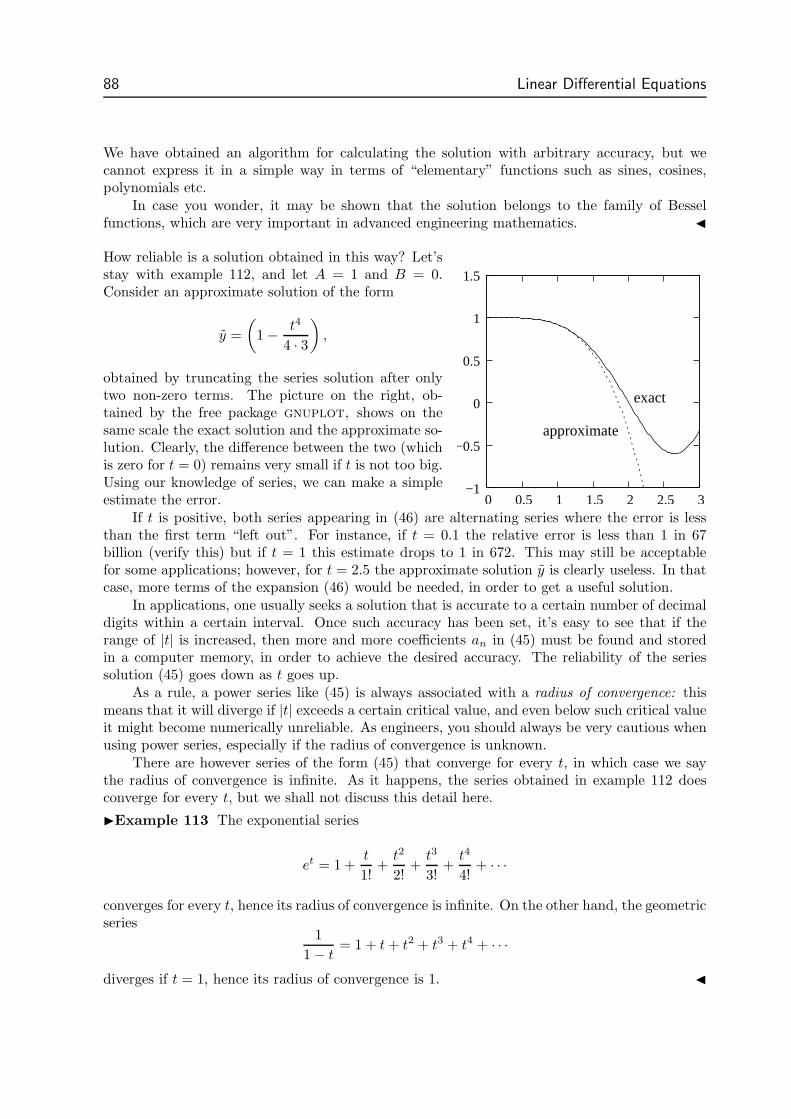
88 Linear Differential Equations
We have obtained an algorithm for calculating the solution with arbitrary accuracy, but wecannot express it in a simple way in terms of “elementary” functions such as sines, cosines,polynomials etc.
In case you wonder, it may be shown that the solution belongs to the family of Besselfunctions, which are very important in advanced engineering mathematics.
How reliable is a solution obtained in this way? Let’sstay with example 112, and let A = 1 and B = 0.Consider an approximate solution of the form
y =
(
1 − t4
4 · 3
)
,
obtained by truncating the series solution after onlytwo non-zero terms. The picture on the right, ob-tained by the free package gnuplot, shows on thesame scale the exact solution and the approximate so-lution. Clearly, the difference between the two (whichis zero for t = 0) remains very small if t is not too big.Using our knowledge of series, we can make a simpleestimate the error.
exact
approximate
−1
−0.5
0
0.5
1
1.5
0 0.5 1 1.5 2 2.5 3If t is positive, both series appearing in (46) are alternating series where the error is less
than the first term “left out”. For instance, if t = 0.1 the relative error is less than 1 in 67billion (verify this) but if t = 1 this estimate drops to 1 in 672. This may still be acceptablefor some applications; however, for t = 2.5 the approximate solution y is clearly useless. In thatcase, more terms of the expansion (46) would be needed, in order to get a useful solution.
In applications, one usually seeks a solution that is accurate to a certain number of decimaldigits within a certain interval. Once such accuracy has been set, it’s easy to see that if therange of |t| is increased, then more and more coefficients an in (45) must be found and storedin a computer memory, in order to achieve the desired accuracy. The reliability of the seriessolution (45) goes down as t goes up.
As a rule, a power series like (45) is always associated with a radius of convergence: thismeans that it will diverge if |t| exceeds a certain critical value, and even below such critical valueit might become numerically unreliable. As engineers, you should always be very cautious whenusing power series, especially if the radius of convergence is unknown.
There are however series of the form (45) that converge for every t, in which case we saythe radius of convergence is infinite. As it happens, the series obtained in example 112 doesconverge for every t, but we shall not discuss this detail here.
Example 113 The exponential series
et = 1 +t
1!+
t2
2!+
t3
3!+
t4
4!+ · · ·
converges for every t, hence its radius of convergence is infinite. On the other hand, the geometricseries
1
1 − t= 1 + t + t2 + t3 + t4 + · · ·
diverges if t = 1, hence its radius of convergence is 1.
Linear Differential Equations 89
Now, let us put this example in a general context.
Definition: A function f(t) is called analytic at a point c if it may be expressed as a powerseries of the form
f(t) = a0 + a1(t − c) + a2(t − c)2 + a3(t − c)3 + a4(t − c)4 + · · ·for all t that are sufficiently near to c.
Clearly, the power series (45) corresponds to the special case where c = 0.
Example 114 Mercator’s Series, which you encountered in first year,
ln t = (t − 1) − (t − 1)2
2+
(t − 1)3
3− (t − 1)4
4+ · · ·
diverges for t = 0 but converges between 0 and 2. Hence, ln t is analytic at t = 1.
We shall not discuss the theory of analytic functions in these notes. One point is worth mention-ing, though: in first year you studied Taylor’s Formula, which allows you to expand a function asa power series using the values of its derivatives at a given point. If a function may be expandedin a Taylor series about c, then it’s obviously analytic at c; it may be shown that the converseis also true, but we’ll skip the proof. In other words, a function is analytic at a given point ifand only if it may be expanded in a Taylor series about that point.
Analytic functions have several important properties. The ones that are crucial for themethod of this section are:
• For a given c, the coefficients an are uniquely determined, and• Power series may be integrated or differentiated term-by-term inside their interval of con-
vergence.
Using these properties, it may be shown that if a linear ODE has an analytic solution at acertain point, and initial conditions are given in the usual way at the same point, then it’spossible to determine the coefficients of the expansion, one after the other, as we have done inexample 112. The first “if” should not be taken for granted. Indeed, some of the most usefulequations in engineering do not meet this requirement. In such cases, the Taylor series methodmust be modified, but you’ll learn about these ideas (Frobenius’ method, Fuchs’ theorem) inother courses.
Example 112 was perhaps easy to follow because the equation was relatively simple. Ingeneral, though, it is better to use a more efficient notation, like in the following examples.
Example 115 Find a solution of the equation ty + 3y − ty = 0.
Solution: We write (45) in summation form:
y(t) =
∞∑
n=0
antn.
To save ourselves some time, let us agree that from now on, whenever the beginning and the endof a sum are not indicated, it’ll be understood that the dummy index runs from zero to infinity.For example, differentiating this equation we get:
y(t) =∑
n
n antn−1
y(t) =∑
n
n(n − 1) antn−2.
90 Linear Differential Equations
Substituting these expressions in the original equation, we get:
∑
n
n(n − 1) antn−1 + 3∑
n
n antn−1 −∑
n
antn+1 = 0.
Now, the first two sums in this expression may be combined into one, but the third sum maynot, because the power tn+1 is not the the same as tn−1. Make sure you understand this
point. It follows that
∑
n
[
n(n − 1) + 3n]
antn−1 −∑
n
antn+1 = 0.
Simplifying, we get:∑
n
n(n + 2) antn−1 −∑
n
antn+1 = 0. (47)
We now note that the powers of t in the two sums in (47) differ by 2 units. If in the first sumwe write n = 2 + m, then n = 0 corresponds to m = −2, and n → ∞ corresponds to m → ∞.So, the first half of (47) may be rewritten as
∑
n
n(n + 2) antn−1 =
∞∑
m=−2
(m + 2)(m + 4)am+2tm+1.
We then separate from the sum on the right, those terms that correspond to a negative m:
∞∑
m=−2
(m + 2)(m + 4)am+2tm+1 = 0 · 2 · a0t
−1 + 1 · 3 · a1t0 +
∞∑
m=0
(m + 2)(m + 4)am+2tm+1.
Going back to (47), we don’t touch the second half, except that we replace the dummy variablen with m. So, (47) becomes
0 · a0t−1 + 3 · a1 +
∑
m
(m + 2)(m + 4)am+2tm+1 −
∑
m
amtm+1 = 0.
Now both sums contain identical powers of t and run from zero to infinity, so we may at lastcombine them into one. It follows that
0 · a0t−1 + 3 · a1 +
∑
m
[
(m + 2)(m + 4)am+2 − am
]
tm+1 = 0.
Proceeding like in example 112, we impose that all monomials vanish separately. Again, thisyields an infinite set of equations:
0 · a0 = 03 · a1 = 0
(m + 2)(m + 4)am+2 − am = 0 [m = 0, 1, 2, 3, . . .]
The first equation is always true, regardless of a0. Hence a0 may take any value: it’s a freeparameter. The second equation is satisfied only if a1 = 0. The other ones yield
am+2 =am
(m + 2)(m + 4). [m = 0, 1, 2, 3, . . .]
Linear Differential Equations 91
In this way, all even coefficients may be computed one after the other. For example, we get
a2 =a0
2 · 4 a4 =a0
2 · 4 · 4 · 6 a6 =a0
2 · 4 · 4 · 6 · 6 · 8 a8 =a0
2 · 4 · 4 · 6 · 6 · 8 · 8 · 10 .
Similarly, from a1 = 0 we get that a3 = 0, hence a5 = 0, and so on: all odd coefficients vanish.It is easy to spot a pattern:
a2 =a0
221! 2!, a4 =
a0
242! 3!, a6 =
a0
263! 4!, a8 =
a0
284! 5!, a10 =
a0
2105! 6!, etc.
So, we may write our solution in compact form:
y = a0 ·∑
m
t2m
22mm! (m + 1)!,
where a0 is free. This is another member of the Bessel functions family.
We mentioned in section 3.3 that the solution space of a 2nd-order linear homogeneous ODEis two-dimensional. Indeed, in example 112 we found two solutions. In this example, instead,we found only one solution (apart from the scalar factor a0). In other words, there are twoindependent solutions but we found only one. This is an unavoidable limitation of the Taylorseries method: the “other” solution was not found because it is not analytic at t = 0. A fulldiscussion of this topic would lead us too far away.
In the next example, two independent solutions are found.
Example 116 Find the solutions of the equation tx − 3x + t5x = 0.
Solution: We repeat all the steps of the preceding example. We write (45) in compact form:
x(t) =∞∑
n=0
antn.
Then, differentiating this equation we get:
x(t) =∑
n
n antn−1
x(t) =∑
n
n(n − 1) antn−2.
Substituting these expressions in the differential equation, we get:
∑
n
n(n − 1)antn−1 − 3∑
n
nantn−1 +∑
n
antn+5 = 0.
Again, we may combine the first two sums; simplifying, we get:
∑
n
[
n(n − 1) − 3n]
antn−1 +∑
n
antn+5 = 0,
∑
n
[
n(n − 4)]
antn−1 +∑
n
antn+5 = 0. (48)
92 Linear Differential Equations
We now note that the powers of t in the two sums in (48) differ by 6 units. Therefore, we mustwrite n = 6 + m in the first sum: in this way n = 0 corresponds to m = −6, and n → ∞corresponds to m → ∞. In other words, we write:
∑
n
[
n(n − 4)]
antn−1 =
∞∑
m=−6
[
(m + 6)(m + 2)]
am+6tm+5.
Now, from the right-hand side we separate the terms that correspond to a negative m:
∞∑
m=−6
(m + 6)(m + 2)am+6tm+5 = 0 · (−4)a0t
−1 + 1 · (−3)a1t0 + 2 · (−2)a2t + 3 · (−1)a3t
2+
+ 4 · 0 · a4t3 + 5 · 1 · a5t
4 +
∞∑
m=0
(m + 6)(m + 2)am+6tm+5.
Going back to (48), in the second sum we replace the dummy index n with m. So, after minorsimplifications, (48) becomes
0a0t−1 − 3a1 − 4a2t − 3a3t
2 + 0a4t3 + 5a5t
4 +∑
m
(m + 6)(m + 2)am+6tm+5 +
∑
m
amtm+5 = 0.
The sums in this equation contain identical powers of t, and m runs from zero to infinity inboth, hence we may combine them. It follows that
0a0t−1 − 3a1 − 4a2t − 3a3t
2 + 0a4t3 + 5a5t
4 +∑
m
[
(m + 6)(m + 2)am+6 + am
]
tm+5 = 0.
We impose that:
0a0 = 0
−3a1 = 0
−4a2 = 0
−3a3 = 0
0a4 = 0
5a5 = 0
(m + 6)(m + 2)am+6 + am = 0 [m = 0, 1, 2, 3, . . .]
We deduce thata0 = free, a4 = free,
because they are multiplied by zero. We also see immediately that it must be
a1 = 0, a2 = 0, a3 = 0, a5 = 0.
All other coefficients are determined by the equation
am+6 = − am
(m + 6)(m + 2)[m = 0, 1, 2, 3, . . .]
Linear Differential Equations 93
We obtain:
a6 = − a0
6 · 2 = −a0
12a12 = − a6
12 · 8 =a0
1152a18 = − a12
18 · 14 = − a0
290304(etc)
and
a10 = − a4
10 · 6 = −a4
60a16 = − a10
16 · 12 =a0
11520a22 = − a16
22 · 18 = − a0
4561920(etc)
All the other coefficients vanish:
am = 0 if m leaves a remainder of 1,2,3 or 5 when divided by 6.
The solution may be left in the form
x = a0
(
1 − t6
12+
t12
1152− t18
290304+ · · ·
)
+ a4
(
t4 − t10
60+
t16
11520− t22
4561920+ · · ·
)
,
where a0 and a4 are free. Clearly the numbers quickly become unwieldy as m grows, but itwould be fairly easy to program a computer to calculate them up to any desired order.
If a solution is a polynomial, the algorithm will stop automatically, once the whole polynomialhas been determined.
Example 117 Find the solutions of the equation (1 + t4)z − 8 t3z + 20 t2z = 0.
Solution: Proceeding like in the preceding examples, we write
z(t) =∑
n
antn,
z(t) =∑
n
nantn−1,
z(t) =∑
n
n(n − 1)antn−2.
Substituting these expressions in the differential equation, we obtain:
∑
n
n(n − 1)antn−2 +∑
n
n(n − 1)antn+2 − 8∑
n
nantn+2 + 20∑
n
antn+2.
The second, third and fourth sums may be combined. It follows:
∑
n
n(n − 1)antn−2 +∑
n
[
n(n − 1) − 8n + 20]
antn+2 = 0,
∑
n
n(n − 1)antn−2 +∑
n
(n2 − 9n + 20) tn+2 = 0.
We now replace n with m + 4 in the first sum, and n with m in the second sum. It follows:
∞∑
m=−4
(m + 4)(m + 3)am+4tm+2 +
∑
m
(m2 − 9m + 20) tm+2 = 0.
94 Linear Differential Equations
Separating the first four terms from the first sum, we obtain (after minor simplifications):
0 a0 t−2 +0 a1 t−1 +2 a2 t0 +6 a3 t1 +
∞∑
m=0
(m+4)(m+3)am+4tm+2 +
∑
m
(m2−9m+20) tm+2 = 0.
At this point the two sums may be combined. We get:
0 a0 t−2 + 0 a1 t−1 + 2 a2 t0 + 6 a3 t1 +∑
m
[
(m + 4)(m + 3)am+4 + (m2 − 9m + 20)am
]
tm+2 = 0.
We impose that
0 a0 = 0
0 a1 = 0
2 a2 = 0
6 a3 = 0
(m + 4)(m + 3)am+4 + (m2 − 9m + 20)am = 0 [m = 0, 1, 2, 3, . . .]
The first two equations yield that
a0 = free, a1 = free.
Similarly, the third and fourth equations yield that
a2 = 0, a3 = 0.
All other coefficients are determined by the equation
am+4 = − (m2 − 9m + 20)
(m + 4)(m + 3)am
= − (m − 4)(m − 5)
(m + 4)(m + 3)am [m = 0, 1, 2, 3 . . .]
Note that, for m = 0, 1, 2, 3, . . . and so on, the denominator of the fraction above is alwayspositive (we never divide by zero). This guarantees that this algorithm may be used indefinitelyto calculate each group of four an’s from the preceding four. For example, substituting m = 0,1, 2 and 3, we get:
a4 = −20
12a0, a5 = −12
20a1, a6 = − 6
30a2 = 0, a7 = − 2
42a3 = 0.
But when we substitute m = 4, 5, 6 and 7 we find that
a8 =0
56a4 = 0, a9 =
0
72a5 = 0, a10 = − 2
90a6 = 0, a11 = − 6
110a6 = 0.
Since we found that four consecutive an’s are zero, it is obvious that all the following ones mustalso be zero. The algorithm stops; the solution, therefore, is simply
z = a0
(
1 − 5t4
3
)
+ a1
(
t − 3t5
5
)
,
Linear Differential Equations 95
where a0 and a1 are free.
Comment: In this example, and in all examples where the solution is a polynomial, the Taylorseries method yields the exact solution, rather than an approximation.
8. Linear ODEs with Variable Coefficients: Special Techniques
REDUCTION OF ORDER
Sometimes, for a given linear homogeneous equation, one may (somehow) find fewer independentsolutions than the order of the equation; in other words, one may get an incomplete solution.For instance, we have seen in the preceding section (example 115) that the Taylor series methodmay fail in this way. In cases like this, it is always possible to use the incomplete solution to geta new differential equation of a lower order.
The method is a simple generalization of Lagrange’s method of variation of parameters.One substitutes
x(t) = u(t) v(t),
x being the original unknown, and v the incomplete solution. Simplifying, one gets an equationof lower order for u. If the original equation was second order, the resulting equation is first-orderlinear, which may then be solved.
Example 118 Solve completely the equation (t+1) x− (3t+4) x +(2t+3)x = 0 given thatit admits the solution v = et.
Solution: Letx = u et x = (u + u) et x = (u + 2u + u) et.
Substituting back and simplifying, we get:
(t + 1) (u + 2u + u) − (3t + 4) (u + u) + (2t + 3)u = 0
(t + 1) u − (t + 2) u = 0.
Note that u has fallen off: this is the main feature of the method of reduction of order, and itmay be used as a check on the calculations. In other words, if u doesn’t fall off there must be amistake.
The last equation is separable; we find that
du
u=
t + 2
t + 1dt =
(
1 +1
t + 1
)
dt.
Integrating, it follows immediately:
ln |u| = t + ln |t + 1| + C,
u = Aet(t + 1),
where A = ±eC is a free constant. Integrating again by parts, it follows that
u = Atet + B.
Finally, recalling that x = u et, we find that the general solution is x = Ate2t + B et.
96 Linear Differential Equations
Example 119 Solve completely the equation t x− (1 + t) x + (34 t−1 + 1
2 )x = 0 given that it
admits the solution v =√
t.
Solution: Let x =√
t u(t); differentiating this expression, one gets
x = t1/2 u =⇒ x = 12 t−1/2 u + t1/2 u =⇒ x = − 1
4 t−3/2 u + t−1/2 u + t1/2 u.
Substituting back into the equation yields:
− 14 t−1/2 u + t1/2 u + t3/2 u −
(
12 t−1/2 u + t1/2 u + 1
2 t1/2 u + t3/2 u)
+ 34 t−1/2 u + 1
2 t1/2 u = 0.
Simplifying, one gets immediately
t3/2 u − t3/2 u = 0
u = u.
The last equation is separable, and it yields immediately
u = Aet =⇒ u = Aet + B.
Hence, the complete solution is x = uv = A√
tet + B√
t.
This procedure is applicable to non-homogeneous linear equations as well, provided an incom-plete solution of the associated homogeneous equation is available. If the original equationwas second-order, then the resulting equation is first-order linear and therefore integrable (seesection 3.6).
Example 120 Solve completely the equation t2y − (t2 + 2t) y + (t + 2) y = t4 given that theassociate homogeneous equation has a solution of the form z = t. (This is example 80.)
Solution: First of all, note that the associate homogeneous equation
t2z − (t2 + 2t) z + (t + 2) z = 0.
may be also solved by the Taylor series method; it’s actually a good revision problem—it yieldsthe general solution. Do it as an exercise.
In this example, let’s pretend that the incomplete solution z = t has been found by inspec-tion. Hence, we let y = u t, where u is the new unknown. Differentiating, it follows:
y = u t + u, y = u t + 2u.
substituting back into the equation, we find:
t2(u t + 2u) − (t2 + 2t) (u t + u) + (t + 2)u t = t4.
Simplifying, we get:
t3u + (2t2 − t3 − 2t2)u + 0 u = t4,
u − u = t.
Linear Differential Equations 97
Note again that u has fallen off, as expected. We now have a first-order linear equation in u,which may be solved by the method variation of parameters (see section 3.6). The letters u andv have alredy been used, though, so instead of (41) we write
u = p q, and hence u = p q + p q.
It follows thatp q +
[
p q − p q]
= t;
solving for q one findsq = et.
Substituting back, one getsp = t e−t,
which (integrating by parts) yields
p = −te−t − e−t + C.
Hence,u = p q = (−te−t − e−t + C) · et = −t − 1 + Cet.
One last integration yieldsu = − 1
2t2 − t + Cet + B,
which finally gives the general solution y = u t = − 12 t3 − t2 + Ctet + Bt.
EULER LINEAR EQUATIONS
The homogeneous Euler equation† is a linear ODE of the form
cntn x(n) + . . . + c2t2 x + c1t x + c0 x = 0,
where c0, c1, c2 etc. are constant. This equation is easy to recognize because the n−th derivativeof the unknown is always multiplied by xn.
An important property of the homogeneous Euler equation is that it always admits a solu-tion of the form x = Atm, where m is a constant to be determined, and A is free. Substituting
x = tm, x = mtm−1, x = m(m − 1)tm−2, and so on,
one gets an equation for m, called indicial equation. The degree of the indicial equation alwaysmatches the order of the differential equation. If the roots are all simple, then the generalsolution is a linear combination of all the solutions found in this way.
Example 121 Solve the equation 2t2x − 9tx + 12x = 0.
Solution: Let x = tm; differentiate with respect to t and substitute back into the equation. Itfollows immediately:
2m(m − 1)tm−2+2 − 9mtm−1+1 + 12tm = 0.
† The term “Euler equations” in engineering has at least three different meanings, as thereare also Euler equations for rigid body motion, and Euler equations for ideal fluids. The Eulerequations discussed here are sometimes called equidimensional Euler or also Euler-Cauchy.
98 Linear Differential Equations
Cancelling the common factor tm, one gets the indicial equation:
2m(m − 1) − 9m + 12 = 0,
2m2 − 11m + 12 = 0.
Solving for m, we obtain m =(
11 ±√
25)
/4, i.e., m = 4 or m = 3/2. The general solution is
therefore x(t) = At4 + Bt3/2.
Example 122 Solve the equation t3 ˙x + t2 x − 6t x + 6x = 0.
Solution: Proceeding as in the previous example, we get the indicial equation:
m(m − 1)(m − 2) + m(m − 1) − 6m + 6 = 0.
This equation is cubic as expected, because the differential equation is third-order. However,it’s easy to spot that a term (m − 1) may be immediately factored out:
m(m − 1)(m − 2) + m(m − 1) − 6(m − 1) = 0
(m − 1) · (m2 − m − 6) = 0.
Hence either m = 1, or m2 − m − 6 = 0; the latter yields m = 3 and m = −2. The generalsolution is therefore x(t) = At + Bt3 + ct−2.
There are two possible problems with this method: complex roots and multiple roots. Complexroots are handled by means of Euler’s formula, as next example shows.
Example 123 Solve the equation t2y + 3ty + 10y = 0.
Solution: Look for solutions of the form y = tm; this leads to the equation
m(m − 1) + 3m + 10 = 0, i.e., m2 + 2m + 1 = −9.
Its solutions are m = −1 ± i3; hence the general solution of this differential equation has theform y = At−1+i3 + B−1−i3. To interpret the imaginary powers, substitute t = eln t and useEuler’s formula. This yields:
ti3 =(
eln t)i3
= ei3 ln t = cos(3 ln t) + i sin(3 ln t).
andt−i3 =
(
eln t)−i3
= e−i3 ln t = cos(3 ln t) − i sin(3 ln t).
So, the general solution may be written y = At−1 cos(3 ln t) + Bt−1 sin(3 ln t).
When the equation for m has multiple roots, the methods explained above yield an incompletesolution. However, reduction of order is always an option.
Example 124 Solve completely the equation t2x − 5tx + 9x = 0.
Solution: Setting x = tm and proceeding like in examples 121–123, we get:
m2 − 6m + 9 = 0.
Linear Differential Equations 99
The indicial equation has the double root m = 3. Therefore, x = t3 is a solution. We need asecond solution; to find it, we let x = t3 u(t) and proceed by reduction of order. Substitutingx = 3t2 + t2 and x = 6t u + 6t2 u + t3 u and simplifying, we get the equation
u + t u = 0,
which is separable:∫
du
u= −
∫
dt
t=⇒ u =
A
t.
Integrating again, we getu = A ln |t| + B,
and finally x = At3 ln |t| + B t3, which is a linear combination of two independent solutions,i.e., the general solution
Example 125 Solve completely the equation 4t2x − 16tx + 25x = 0.
Solution: We get the indicial equation 4(
m2 − 5m + 254
)
= 0, which has the double root m = 52.
Letting x = t5/2u(t) and proceeding by reduction of order (do it, as an exercise), one eventuallygets the general solution in the form x = At5/2 ln t + B t5/2.
It may be shown that if the indicial equation has a double root m = k, then the correspondingEuler equation has always two solutions of the form tk and tk ln t. We’ll look into the proof,because it is a good revision example in the calculus of several variables.
Consider a generic 2nd-order Euler equation:
c2t2 x + c1t x + c0 x = 0
where c2, c1 and c0 are constant. We want to see if it has a solution of the form x = tm ln t.This means we want to see under what conditions the equation
c2t2 d2(tm ln t)
dt2+ c1t
d(tm ln t)
dt+ c0(t
m ln t) = 0
holds identically for every t. The crucial point is the observation that
tm ln t =∂ tm
∂m;
convince yourself of this. So, the previous equation is equivalent to
c2t2 d2
dt2
[
∂ tm
∂m
]
+ c1td
dt
[
∂ tm
∂m
]
+ c0
[
∂ tm
∂m
]
= 0.
Since differentiation with respect to m and differentiation with respect to t are interchangeable,this may also be written
∂
∂m
[
c2
(
t2d2 tm
dt2
)
+ c1
(
td tm
dt
)
+ c0tm
]
= 0,
100 Linear Differential Equations
and hence∂
∂m
[
c2m(m − 1)tm + c1mtm + c0tm
]
= 0. (49)
Now, if the indicial equation has two simple roots m = k and m = l, then it may be writtenc2(m − k)(m − l) = 0. If, however, has only one double root m = k, then it must have the form
c2(m − k)2 = 0.
In this second case, (49) becomes
∂
∂m
[
c2(m − k)2tm]
= 0,
2c2(m − k) tm + c2(m − k)2tm ln t = 0.
It’s evident that the left-hand side is identically zero if m = k. Therefore the function x = tk ln tfits the equation, i.e., it is a solution. As an exercise, show that this is not true in the case oftwo simple roots.
Conclusion: If m = k is a double root of the indicial equation, then the Euler equation hastwo independent solutions of the form tk and tk ln t.
This proof may be easily adapted to Euler equations of 3rd-order (where the indicial equationmay have three simple roots, or a double root plus a simple root, or one triple root), and higherorder. The details are essentially the same.
For instance, it may be shown that if m = k is a triple root, then the Euler equation hasthree independent solutions of the form tk, tk ln t and tk(ln t)2. Similarly, if m = k is a quadrupleroot, then one gets the expressions listed above, plus a fourth solution of the form tk(ln t)3. Therule is extended in the same way to roots of higher algebraic multiplicity.
Example 126 Solve completely t3 ˙x + t x + 1.
Solution: The indicial equation is
m(m − 1)(m − 2) + m − 1 = 0,
m3 − 3m2 + 3m − 1 = 0,
i.e., (m − 1)3 = 0. Hence, the general solution is x = At + B t ln t + C t(ln t)2.
Example 127 Find all the solutions of t4 x(4) + 4t3 ˙x + t2 x + t x − x = 0 [for t > 0].
Solution: We get the indicial equation
m(m − 1)(m − 2)(m − 3) + 4m(m − 1)(m − 2) + m(m − 1) + m − 1 = 0,
which factors immediately as (m − 1)[m3 − m2 − m + 1] = (m − 1) [m2(m − 1) − (m − 1)] =(m − 1)3(m + 1) = 0. Hence, we find two roots, m = 1 (triple) and m = −1 (simple). Thegeneral solution is x = At + B t ln t + C t(ln t)2 + D t−1. Four terms, of course.
Linear Differential Equations 101
THE LAPLACE TRANSFORM
Occasionally, if the coefficients are polynomials in t, the Laplace transform may be used becausemultiplication of x(t) by t corresponds to differentiation of X(s). In this way, a differentialequation of order n for x(t) is turned into a differential equation of order m for X(s), where mis the highest power of t appearing in the original equation. If m < n this may be a step towardthe solution.
Example 128 Solve tx − (t + 1)x + x = 0.
Solution: This is a second-order linear equation with non-constant coefficients. Writing
L[
x(t)]
= X(s),
L[
x(t)]
= sX(s) − a,
L[
x(t)]
= s2X(s) − sa − b,
and recalling the operator identity (17)
t· ↔ − d
ds,
we get
− d
ds
(
s2X − sa − b)
+d
ds
(
sX − a)
−(
sX − a)
+ X = 0.
It follows that
−2sX − s2X ′ + a + X + sX ′ − sX + a + X = 0,
(s2 − s)X ′ + (3s − 2)X = 2a.
We have obtained a first-order linear equation for X, which may be solved by the method ofvariation of parameters: writing
X(s) = U(s)V (s)
and substituting, it follows
s(s − 1)U ′V +[
s(s − 1)UV ′ + (3s − 2)UV]
= 2a.
Imposing that the part in brackets vanish:
s(s − 1)UV ′ + (3s − 2)UV = 0,
canceling U and solving, we get
∫
dV
V=
∫
2 − 3s
s(s − 1)ds = −
∫(
2
s+
1
s − 1
)
ds.
Integrating, it follows that
V =1
(s − 1)s2,
102 Linear Differential Equations
and substituting back:
s(s − 1)U ′ · 1
(s − 1)s2= 2a.
Hence,
U ′ = 2as
U = as2 + c,
where c is the integration constant. We then find X:
X = UV =as2 + c
(s − 1)s2=
=a + c
s − 1− c
s− c
s2.
Since a has not been specified anyway, we may re-define a + c; finally, we get
x = L−1[
X]
= c1et − c2(t + 1).
A REVISION EXAMPLE
Example 129 Find the general solution of t2y − 2y = ln t.
Solution: This is a non-homogeneous equation. The associate homogeneous equation is
t2z − 2z = 0,
which is of the Euler type. It has solutions of the form tm, where m is given by the indicialequation m(m − 1) − 2 = 0. Solving it, we find m = 2 or m = −1.
We proceed by reduction of order, setting y = uv, where v = t2 or v = t−1. Eithersubstitution would work; let us say, y = t2u. It follows that y = t2u + 4tu + 2u; substitutinginto the original equation, we obtain:
t2(t2u + 4tu + 2u) − 2t2u = ln t.
Simplifying, we get:t4u + 4t3u = ln t.
This is first-order linear in u, so (by the method of variation of parameters) we set
u = wx, u = wx + wx.
Substituting back, we get:
t4wx +[
t4wx + 4t3wx]
= ln t.
We impose that the expression in square brackets vanish, and we get an equation for x :
tx + 4x = 0.
Solving it, we find x = t−4; substituting back we get an equation for w:
t4wt−4 = ln t.
Linear Differential Equations 103
Solving this one, we find w = t ln t − t + C. We now have an equation for u:
u = wx = (t ln t − t + C) · t−4 =
= t−3 ln t − t−3 + Ct−4.
Integrating, we get:u = − 1
2t−2 ln t − 1
4t−2 + 1
2t−2 − 1
3Ct−3 + B =
= − 12 t−2 ln t + 1
4 t−2 + At−3 + B,
where A and B are free. Finally, from y = uv, we get
y = ut2 = − 12 ln t + 1
4 + At−1 + Bt2,
and this is the general solution.
9. Systems of Linear ODEs
Systems of linear equations with constant coefficients may be handled by the Laplace transformexactly as you would expect: by transforming the system of differential equations in x, y, z, . . .into a system of algebraic equations in X, Y , Z, . . .. Initial conditions (if given) are accounted forin a natural way; there is really nothing new to learn. The homogeneous and non-homogeneoussystems correspond, respectively, to homogeneous and non-homogeneous equations, and all thecomments made in sections 3.2–5 apply to systems as well.
Example 130 Solve the system
x + 2x + y = e−t
y − x = 0,with initial values x(0+) = y(0+) = 0.
Solution: Taking the Laplace transform of the system, we get
sX + 2X + Y = 1/(s + 1)
sY − X = 0.
This is a system of 2 algebraic equations with 2 unknowns, described by the augmented matrix
[
s + 2 1−1 s
∣
∣
∣
∣
1/(s + 1)0
]
,
where the coefficients are parametrized by s. Solving it by Cramer’s rule, we get:
X(s) =
∣
∣
∣
∣
1/(s + 1) 10 s
∣
∣
∣
∣
∣
∣
∣
∣
s + 2 1−1 s
∣
∣
∣
∣
=s/(s + 1)
s2 + 2s + 1=
s
(s + 1)3.
Simplifying, it follows that
X(s) =s + 1 − 1
(s + 1)3=
1
(s + 1)2− 1
(s + 1)3.
104 Linear Differential Equations
In the same way, we get:
Y (s) =
∣
∣
∣
∣
s + 2 1/(s + 1)−1 0
∣
∣
∣
∣
∣
∣
∣
∣
s + 2 1−1 s
∣
∣
∣
∣
=1
(s + 1)3.
Finally, inverting the Laplace transforms, we obtain:
x(t) = te−t − 12 t2e−t, y(t) = 1
2 t2e−t.
Example 131 In theoretical mechanics, Euler’s equations for a free symmetric rotor may be
reduced to a system of the form
ω1 = −kω2
ω2 = kω1,where k is a constant determined by the rotor’s
principal moments. Solve the system, given ω1(0+) = 1, ω2(0+) = 0.
Solution: Taking the Laplace transform of the equations, we get
sΩ1 − 1 = −kΩ2
sΩ2 = kΩ1.
It follows by Cramer’s rule that
Ω1(s) =
∣
∣
∣
∣
1 k0 s
∣
∣
∣
∣
∣
∣
∣
∣
s k−k s
∣
∣
∣
∣
=s
s2 + k2,
Ω2(s) =
∣
∣
∣
∣
s 1−k 0
∣
∣
∣
∣
∣
∣
∣
∣
s k−k s
∣
∣
∣
∣
=k
s2 + k2,
and finally that
ω1(t) = cos kt, ω2(t) = sin kt.
Example 132 The system
5x1 = −36x1 + 4(x2 − x1)
0.8x2 = −4(x2 − x1)describes the motion of a double
harmonic oscillator [if for example the oscillating masses are 5 kg and 0.8 kg and the two springshave stiffness 36N/m and 4N/m, respectively]. Given that initially x1(0) = x2(0) = x1(0) = 0,and x2(0) = −1.25m/s, determine the motion of the system.
Solution: Taking the Laplace transform of the equations of motion, we get
5s2X1 = −40X1 + 4X2
0.8(s2X2 + 1.25) = 4X1 − 4X2.
Linear Differential Equations 105
Simple manipulations yield the augmented matrix
[
5s2 + 40 −4−4 0.8s2 + 4
∣
∣
∣
∣
0−1
]
.
The determinant of the coefficient matrix is
D(s) = (5s2 + 40) (0.8s2 + 4) − 16 = 4s4 + 52s2 + 144 = 4(s2 + 9)(s2 + 4).
Solving the system by Cramer’s rule, we get
X1(s) =
∣
∣
∣
∣
0 −4−1 0.8s2 + 4
∣
∣
∣
∣
4(s2 + 9)(s2 + 4)=
−4
4(s2 + 9)(s2 + 4).
Expanding in partial fractions, we get
X1(s) =15
s2 + 9−
15
s2 + 4,
and finallyx1(t) = 1
15sin 3t − 1
10sin 2t.
Similarly, we get:
X2(s) =
∣
∣
∣
∣
5s2 + 40 0−4 −1
∣
∣
∣
∣
4(s2 + 9)(s2 + 4)=
−5s2 − 40
4(s2 + 9)(s2 + 4).
Expanding in partial fractions, we obtain:
X2(s) = −14
s2 + 9− 1
s2 + 4,
finally:x2(t) = − 1
12sin 3t − 1
2sin 2t.
Example 133 Solve the system
x = 8x − 7y − 7z
y = 10x − 9y − 10z
z = −2x + 2y + 3z,
with initial values
x(0+) = 2,
y(0+) = 1,
z(0+) = 0.
Solution: Taking the Laplace transform of the system and rearranging the system we get
(s − 8)X + 7Y + 7Z = 2
−10X + (s + 9)Y + 10Z = 1
2X − 2Y + (s − 3)Z = 0
The determinant of this system is
∣
∣
∣
∣
∣
∣
(s − 8) 7 7−10 (s + 9) 102 −2 (s − 3)
∣
∣
∣
∣
∣
∣
= (s − 8)
∣
∣
∣
∣
(s + 9) 10−2 (s − 3)
∣
∣
∣
∣
+ 10
∣
∣
∣
∣
7 72 (s − 3)
∣
∣
∣
∣
+ 2
∣
∣
∣
∣
7 7(s + 9) 10
∣
∣
∣
∣
=
106 Linear Differential Equations
= (s − 8)(s2 + 6s − 7) + 70(s − 1) − 14(s − 1) = (s − 1) ·(
(s − 8)(s + 7) + 56)
= s(s − 1)2.
Solving for X by Cramer’s rule we get:
X(s) =
∣
∣
∣
∣
∣
∣
2 7 71 (s + 9) 100 −2 (s − 3)
∣
∣
∣
∣
∣
∣
s(s − 1)2=
(2s + 7)(s − 1)
s(s − 1)2=
2s + 7
s(s − 1)=
9
s − 1− 7
s.
It follows immediately that
x(t) = 9et − 7.
Similarly, we find that
Y (s) =
∣
∣
∣
∣
∣
∣
(s − 8) 2 7−10 1 102 0 (s − 3)
∣
∣
∣
∣
∣
∣
s(s − 1)2=
(s + 10)(s − 1)
s(s − 1)2=
s + 10
s(s − 1)=
11
s − 1− 10
s
and
Z(s) =
∣
∣
∣
∣
∣
∣
(s − 8) 7 2−10 (s + 9) 12 −2 0
∣
∣
∣
∣
∣
∣
s(s − 1)2=
2(1 − s)
s(s − 1)2= − 2
s(s − 1)=
2
s− 2
s − 1.
It follows immediately that y(t) = 11et − 10 and z(t) = 2 − 2et.
Differential equations of order n, and systems of n equations of order 1, are two sides of thesame coin, so to speak, as the following example illustrates.
Example 134 Write the third-order differential equation ˙x− 3x+ 3x−x = t2et, as a systemof first-order equations.
Solution: Define x = y, x = y = z; we get immediately
x = y,
y = z
z = 3z − 3y + x + t2et;
this may be re-written in matrix form
xyz
=
0 1 00 0 11 −3 3
xyz
+
00
t2et
.
It is possible to show that the eigenvalue equation for the square matrix appearing above isformally the same as the characteristic equation D(s) = 0 of the original equation: specifically,
D(s) = s3 − 3s2 + 3s − 1 = (s − 1)3,
Linear Differential Equations 107
and∣
∣
∣
∣
∣
∣
−λ 1 00 −λ 11 −3 3 − λ
∣
∣
∣
∣
∣
∣
= −(λ − 1)3.
Note that the only root is s = 1, with algebraic multiplicity 3. Go back to example 100 for asolution of this problem.
In exactly the same way, an equation of order n may be converted into a system of n first-order equations (convince yourself of this). If, in addition, the equation is linear with constantcoefficients, then its characteristic equation is converted into the eigenvalue equation for thecorresponding matrix.
Therefore, the study of differential equations of order n may be seen as a special case ofthe theory of linear systems of order 1: this is an important result from a theoretical point ofview, but in practice, solving a single equation of order n requires probably no more work thansolving the corresponding n ∗ n system. So, converting high-order equations into first-ordersystems is not necessarily a step forward towards the solution.
10. Convolution Integral Equations
Equations of the form
∫ t
0
K(t − τ)x(τ) dτ = f(t),
x(t) +
∫ t
0
K(t − τ)x(τ) dτ = f(t),
where f(t) and K(t) are given functions, x(t) is unknown, represent an important class ofintegral equations. The function K(t) is called the kernel of the equation. Recalling that theLaplace transform of a convolution product is the (ordinary) product of the tranforms, we seeimmediately that the Laplace transform is well suited for this kind of problems. Leaving asidequestions such as existence and uniqueness of solutions and other theoretical features, let us seehow the method works in practice.
Example 135 Solve the integral equation∫ t
0et−τx(τ) dτ = sin t.
Solution: The equation may be written
et ∗ x(t) = sin t;
taking the Laplace transform of the equation, we get
X(s)
s − 1=
1
s2 + 1.
It follows immediately
X(s) =s − 1
s2 + 1,
and hencex(t) = cos t − sin t.
108 Linear Differential Equations
Example 136 Solve the integral equation x(t) = cos t +∫ t
0(t − τ)x(τ) dτ .
Solution: Transforming the equation
x(t) = cos t + t ∗ x(t)
we get
X(s) =s
1 + s2+
X(s)
s2.
It follows immediately
X(s) =s3
(s2 + 1)(s2 − 1)=
12s
s2 + 1+
12s
s2 − 1,
and finallyx(t) = 1
2 cos t + 12 cosh t.
Example 137 Solve the integral equation x(t) = t +∫ t
0sin(t − τ)x(τ) dτ .
Solution: Transforming the equation
x(t) = t + sin t ∗ x(t),
we get
X(s) =1
s2+
X(s)
1 + s2,
and hence
X(s) =1 + s2
s4=
1
s4+
1
s2.
Finally, the solution isx(t) = 1
6 t3 + t.
11. Additional Examples
All the “special tecniques” discussed so far may be extended in a natural way to equations ofhigher order and to systems. The next couple of examples deal with third-order equations.
Example 138 The equation t3 ˙x − 3t2x + t(6 − t2)x − (6 − t2)x = 0 admits an incompletesolution of the form x = t. Find the general solution.
Solution: The incomplete solution is not hard to spot: the term (6 − t2) appearing twice, givesit away. So, letting
x(t) = t u(t)
and differentiating, we get:
x = t u + u x = t u + 2u x = t ˙u + 3u.
It follows immediately:
t3(t ˙u + 3u) − 3t2(tu + 2u) + t(6 − t2)(tu + u) − (6 − t2)tu = 0.
Linear Differential Equations 109
Simplifying, we get:t4 ˙u − t4u = 0,
˙u − u = 0.
Having started with a third order equation, we have obtained a second order equation in u,which may be solved immediately:
u = A cosh t + B sinh t,
where A and B are free. Integrating again, we find that
u = A sinh t + B cosh t + C.
So, finally, the general solution is x = At sinh t + Bt cosh t + Ct.
Example 139 Apply the Taylor series method to the equation t2 ˙x + tx + x = 0.
Solution: Proceeding like in section 3.7, we write:
x =∑
n
antn, x =∑
n
anntn−1, x =∑
n
ann(n−1)tn−2, ˙x =∑
n
ann(n−1)(n−2)tn−3.
Substituting these expressions into the equation, we get:
∑
n
ann(n − 1)(n − 2)tn−1 +∑
n
anntn +∑
n
antn = 0.
Substituting n = m + 1 in the first sum, and grouping the other two sums, we get:
∞∑
m=−1
am+1(m + 1)m(m − 1)tm +∑
m
am(m + 1)tm = 0.
Detaching the first term of the first sum, it follows:
0 · a0t−1 +
∑
m
[
am+1(m + 1)m(m − 1) + am(m + 1)]
tm = 0.
This equation is identically satisfied if0 · a0 = 0
andam+1(m + 1)m(m − 1) + am(m + 1) = 0 [m = 0, 1, 2, 3, . . .]
The first equation is satisfied regardless of the value of a0. Proceeding with the other equations,we find that the next two are special:
0 · a1 + a0 = 00 · a2 + 2a1 = 0
am+1(m + 1)m(m − 1) + am(m + 1) = 0
[m = 0 ][m = 1 ]
[m = 2, 3, . . . ]
The first equation from this set fixes a0, regardless of the value of a1:
a0 = 0.
110 Linear Differential Equations
So, a0 is not free. Similarly, the second equation fixes a1, regardless of the value of a2:
a1 = 0.
If m > 1, then certainly m(m − 1) in not zero, hence simplifying we obtain the algorithm
am+1 = − am
m(m − 1)[m = 2, 3, . . .]
which yields all other coefficients. However, there is no equation for a2, hence a2 is free. Forinstance, we get
a3 = − a2
2 · 1 a4 = +a2
3 · 2 · 2 · 1 a5 = − a2
4 · 3 · 3 · 2 · 2 · 1
and so forth. The solution thus found may be written
x = a2
(
t2 − t3
2! 1!+
t4
3! 2!− t5
4! 3!+
t6
5! 4!− t7
6! 5!+ · · ·
)
.
Note that the given equation must have three independent solutions, and we only found one.This means that the other solutions do not have a Taylor series about x = 0.
Example 140 A simple harmonic oscillator having mass m = 4 kg and spring constant κ = 16N/m, initially at rest, is pulled by a constant force f0 = 8 N for 6 seconds and then released.Describe the subsequent motion.
Solution: Let y be the displacement from equilibrium. The equation of motion is
my + κy =
0 if t < 0,f0 if 0 < t < 6,0 if t < 0.
Substituting m = 4, κ = 16 and f0 = 8 and simplifying, we obtain the equation
y + 4y = 2[
u(t) − u(t − 6)]
,
where u(t) is Heaviside’s step function. The initial conditions are: y(0+) = 0, y(0+) = 0.The transformed equation is
(s2 + 4)Y (s) = 2 · 1 − e−6s
s.
It follows:
Y (s) =2(1 − e−6s)
s(s2 + 4).
Now, we observe that
L−1
[
2
s(s2 + 4)
]
=
∫ t
0
sin 2τ dτ = 12 (1 − cos 2t).
Linear Differential Equations 111
Then, by the t-shift property (20), we get
y(t) = 12u(t) (1 − cos 2t) − 1
2u(t − 6) (1 − cos 2(t − 6)) =
=
0 if t < 0,12 (1 − cos 2t) if 0 < t < 6,12 (1 − cos 2t) − 1
2
(
1 − cos 2(t − 6))
if t > 6.
Applying the identity cosA − cos B = −2 sin 12 (A + B) sin 1
2 (A − B), we finally get:
y(t) =
0 if t < 0,sin2 t if 0 < t < 6,sin 6 sin(2t − 6) if t > 6.
Note that the solution is continuous throughout.
Next example is a continuation of the preceding one.
Example 141 Suppose the oscillator considered in example 140 is initially at 2 m from theequilibrium point, moving toward it with speed 3 m/s. Starting at time t = 0, the oscillator ispulled by a constant force f0 = 8 N for 6 seconds and then released. Describe the subsequentmotion.
Solution: The equation of motion is the same as in example 140; only the initial conditions differ.So, let us call x the solution of this problem, and y the solution found in example 140.
The associate homogeneous equation is 4z + 16z = 0. and its general solution is quicklyfound to be
z = A cos 2t + B sin 2t
(convince yourself of this). So, the general solution of this problem is
x(t) = A cos 2t + B sin 2t + y(t),
where y(t) is the solution found in example 140. We now require that x(0+) = 2 and x(0+) = −3.Recalling that y(0+) = 0 and y(0+) = 0, these conditions yield:
A cos 0 + B sin 0 + 0 = 2, −2A sin 0 + 2B cos 0 + 0 = −3.
It follows immediately that A = 2 and B = − 32 ; finally, the complete solution is
x = y + z =
0 if t < 0,
2 cos 2t − 32 sin 2t + sin2 t if 0 < t < 6,
2 cos 2t − 32 sin 2t + sin 6 sin 2(t − 3) if t > 6.
Example 142 Solve completely the equation tx + 2x + tx = 0.
Solution: Taking the Laplace transform of the equation, and writing x(0+) = a, x(0+) = b,we get
− d
ds
(
s2X − sa − b)
+ 2sX − 2a − dX
ds= 0,
112 Linear Differential Equations
which yields
−s2X ′ − 2sX + a + 2sX − X ′ = 0,
X ′ =a
1 + s2.
Imposing that X(∞) = 0, it follows that
X = −a
∫ ∞
s
dσ
1 + σ2.
Finally, by the methods of chapter 2, we get
x(t) = −a · sin t
t.
Since in the process of finding X(s) the constant b dropped off, this solution is incomplete. So,we write
v(t) =sin t
t
andx = uv, =⇒ x = uv + uv, =⇒ x = uv + 2uv + uv.
Replacing these expressions in the original equation, we get
t(uv + 2uv + uv) + 2(uv + uv) + tuv = 0,
oru tv + 2u(tv + v) + u(tv + 2v + tv) = 0.
Now, use the fact that v = sin t/t is a solution of the equation, i.e. that
tv + 2v + tv = 0.
Simplifying, we getu
u= −2(vt + v)
vt= −2 cos t
sin t.
This is immediately integrable:
ln |u| = −2 ln | sin t| + ln |c|,
where c is a constant, hence
u =c
sin2 t, =⇒ u = −c cot t + a,
where a is another constant. Finally, we put u and v together:
x = (−c cot t + a) · sin t
t= −c · cos t
t+ a · sin t
t.
Linear Differential Equations 113
We now have two independent solutions, namely sin t/t and cos t/t. Note that the secondsolution, cos t/t, does not have a Laplace transform [the integral (3) would diverge]: this is whywe failed to find it by such a method.
Example 143
Solve the system of integral equations
x(t) = et +∫ t
0x(τ) dτ −
∫ t
0e(t−τ)y(τ) dτ,
y(t) = −t −∫ t
0(t − τ)x(τ) dτ +
∫ t
0y(τ) dτ.
Solution: Transforming the system, we get
X(s) =1
s − 1+
X(s)
s− Y (s)
s − 1,
Y (s) = − 1
s2− X(s)
s2+
Y (s)
s.
Solving this system, we get
X(s) =s(s − 1) + 1
(s − 1)3 − 1=
s2 − s + 1
(s − 2)(s2 − s + 1)=
1
s − 2,
Y (s) =−(s − 1)2/s − 1
(s − 1)3 − 1= − s2 − s + 1
s(s − 2)(s2 − s + 1)=
12
s−
12
s − 2.
Finally, we getx(t) = e2t,
y(t) = 12 − 1
2e2t.
114 Tutorial Problems Linear Differential Equations
PROBLEMS
Homogeneous Linear ODEs with Constant Coefficients
34. Find the general solution of the following linear ODEs with constant coefficients.(a) x − 7x + 10x = 0
(b) x(4) + 8x(2) + 16x = 0
(c) ˙x − 6x + 12x − 8x = 0
(d) 4x − 8x + 1 = 0
35. Find the general solution of the following linear ODEs with constant coefficients.
(a) x(6) + 300x(4) + 30 000x(2) + 1 000 000x = 0(b) x(8) − 8x(4) + 16x = 0(c) ˙x + 8x = 0(d) ˙x − x + 81x − 81x = 0
Non-Homogeneous Linear ODEs with Constant Coefficients
36. Find the general solution of the following linear ODEs with constant coefficients.(e) x − x = et
(f) x + x − 6x = t e2t
(g) x(4) + 4x(3) + 6x(2) + 4x(1) + x = e−t sin t
(h) ˙x + 11x − x − 11x = e−11t
Linear ODEs with Constant Coefficients: Initial-Value Problems
37. Solve the following initial-value problems.(a) x + x = e−t, x0 = 1
(b) x + x = 0, x0 = 1, x0 = 0
(c) x − 2x + 2x = 1, x0 = x0 = 0
(d) x + 2x + x = t2, x0 = 1, x0 = 0
(e) x + 4x = t, x0 = 1, x0 = 0
(f) x − 2x + 5x = 1 − t, x0 = x0 = 0
38. Solve the following initial-value problems.
(a) x + 9x =
1 if 0 < t < 2,0 everywhere else; x(0+) = 0, x(0+) = 0.
(b) x + 2x =
t if 0 < t < 1,0 everywhere else; x(0+) = 0.
A View From Above
39. For the following problems, use the Green’s function method (39) to find the particularsolution that satisfies the initial conditions y(0+) = y(0+) = 0.
(a) y − y = tanh t,
(b) y + y = 1/ cos t,
(c) y − y = 1/ cosh3 t,
(d) y + y = 1/(1 + cos t).
Linear First-order ODEs with Variable Coefficients
40. Find the general solution of the following equations.(a) x − x/t = t(b) tx − 3x = e1/t
(c) (t2 − 1)x + tx =√
t − 1
(d) cosh2 t · y − y = tanh2 t(e) (t2 + 1)y + ty = (1 − 2t)
√t2 + 1
(f) (1 + t2)y + y = arctan t
Linear Differential Equations Tutorial Problems 115
41. Solve the following initial-value problems(a) (1+ t)4 y+3(1+ t)3y = 1+ t+ t2, y(0) = 0(b) tx − x = t3 + 3t2 − 2t, x(1) = 4
(c) x − x tan t = t, x(0) = 8(d) x ln t + 2x/t = 1, x(e) = 3
42. Show that Lagrange’s method of variation of parameters (i.e., substituting x = uv) worksjust as well for the so-called Bernoulli equation ax + bx = cxp, where a, b and c are functionsof t and p is a (constant) power. The first-order linear equation corresponds to the special casep = 0 of the Bernoulli equation.
43. Solve the following Bernoulli equations.(a) tx−2x = 3t2x−1, (b) x tanh t−x = tx2. (c) 3tx−(1+ t sin t)x = −3x4 sin t.
Taylor Series Method
44. Use the Taylor series method to solve the following equations.(a) x − x = 0(b) t y + y − 4t y = 0(c) (t − t2) z − 3z + 2z = 0
(d) x − t2x − 2t x = 0(e) t2y − 2t y + (2 + t2)y = 0(f) z − t z + 6z = 0
Reduction of Order
45. Find the general solution of (t − 4)x − (t − 3)x + x = 0, given that it has an incompletesolution of the form x = et.
46. Find the general solution of x + (1 − 2 tanh2 t)x = 0, given that it has an incompletesolution of the form x = 1/ cosh t.
47. Find the general solution of x t2 cos t + x t(t sin t− 2 cos t) + x (2 cos t− t sin t) = 0, giventhat it has an incomplete solution of the form x = t.
48. Find the general solution of x cosh2 t + 2x = 0, given that it has an incomplete solutionof the form x = tanh t.
49. Verify that the equation tx− (t+2)x+3x = 0 has a solution of the form x = t3. Hence,using reduction of order, show that the general solution is x = At3 + Bt3
∫
(et/t4) dt.
50. Find the general solution of t3 ˙x− 3t2x + t(6 + t2)x− (6 + t2)x = 0, given that it has anincomplete solution of the form x = t.
Euler Equidimensional Equations
51. Solve the following Euler equations.(a) 2t2x + 3tx − x = 0(b) t3 ˙x−2t2x−5tx+5x = 0
(c) t2x+5tx+4x = 0(d) t2x+ tx+49x = 0
(e) t3 ˙x + 170tx − 170x = 0(f) t3 ˙x + 3t2x + tx = 0
52. Solve the following Euler equations.(a) (t + 4)2 x + 6(t + 4) x + 6x = 0 Hint: Substitute t + 4 = τ .(b) (t + 2)2 x + (t + 2) x + π2x = 0 Hint: Substitute t + 2 = τ .
53. Double complex roots: solve t4 x(4) + 6t3 x(3) + 11t2 x(2) + 5t x(1) + 4x = 0.
Special Techniques
54. Take the Laplace transform of the following equations, solve for X(s) and hence find x(t).(a) tx + (t − 1)x − x = 0; x0 = 5, x0 = −5.(b) (2t + 1)x − 2x − (2t + 3)x = 0; x0 = 0, x0 = 1.
116 Tutorial Problems Linear Differential Equations
55. Take the Laplace transform of the following equations, solve for X(s) and hence find thegeneral solution.
(a) tx − 2x − tx = 0
(b) t ˙x − x − tx + x = 0.
56. Solve problem 54(a) by the Taylor series method and verify that you get the same answer.
Systems of ODEs
57. Solve the following initial-value problems.
(a)
x + y = 0,y + x = 0,
x0 = 1
y0 = −1
(b)
x = −2x + y,y = −5x + 4y,
x0 = 1
y0 = 3
(c)
x = 5x − y,y = 3x + y,
x0 = 2
y0 = −1
(d)
x − y − 2x + 2y = 1 − 2t,x + 2y + x = 0,
x0 = x0 = 0
y0 = 0
58. Solve the following initial-value problems.
(a)
x = −2x − 2y − 4z,y = −2x + 2y − 2z,z = 5x + 2y + 7z
x0 = 1
y0 = 1
z0 = 1
(b)
x − x + y + 2y = 1 + et,y + 2y + z + z = 2 + et,x − x + z + z = 3 + et
x0 = 0
y0 = 0
z0 = 2
Convolution Integral Equations
59. Solve the following equations.
(a) x(t) = 1+ 16
∫ t
0
(t−τ)3x(τ) dτ
(b)
∫ t
0
cos(t − τ)x(τ) dτ = t + t2
(c)
∫ t
0
cosh(t − τ)x(τ) dτ = t
(d) x(t) = t + 2
∫ t
0
(
t − τ − sin(t − τ))
x(τ) dτ
60. Solve the following system of integral equations.
x(t) = 2 −∫ t
0
(t − τ)x(τ) dτ − 4
∫ t
0
y(τ) dτ
y(t) = 1 −∫ t
0
x(τ) dτ −∫ t
0
(t − τ) y(τ) dτ
ANSWERS
34 (a) Ae2t + Be5t
(b) A cos 2t+B sin 2t+Ct cos 2t+Dt sin 2t
(c) e2t(A + Bt + Ct2)
(d) et(A cosh√
3t/2 + B sinh√
3t/2)
35 (a) (A + Bt + Ct2) cos 10t + (D + Et + Ft2) sin 10t(b) (A + Bt) cosh
√2t + (C + Dt) sinh
√2t + (E + Ft) cos
√2t + (G + Ht) sin
√2t
(c) Ae−2t + B et cos√
3t + C et sin√
3t(d) Aet + B cos 9t + D sin 9t.
36 (e) Aet + Be−t + 12 tet
(f) Ae2t + Be−3t + 110 t2e2t − 1
25 te2t
(g) e−t(A + Bt + Ct2 + Dt3) + e−t sin t
(h) Aet + Be−t − Ce−11t + 1120 t e−11t
37 (a) (t + 1)e−t
(b) cos t
(c) 12 + 1
2et(sin t − cos t),
(d) t2 − 4t + 6 − e−t(5 + t)
(e) 14 t + cos 2t − 1
8 sin 2t
(f) 325 − 1
5 t − 125et
(
3 cos 2t − 4 sin 2t)
Linear Differential Equations Tutorial Problems 117
38 (a) x =
0 if t ≤ 0,19 (1 − cos 3t) if 0 < t < 2,19 (cos 3t · cos 6 + sin 3t · sin 6 − cos 3t) if t ≥ 2.
(b) x =
0 if t ≤ 0,(e−2t − 1 + 2t)/4 if 0 < t < 1,e−2t(1 + e2)/4 if t ≥ 1.
39 (a) y = − sinh t+cosh t·arctan(sinh t)(b) y = t sin t + cos t · ln | cos t|
(c) y = 12 sinh t · tanh t
(d) y = sin t·(
t−tan 12 t
)
+cos t·ln(
12 + 1
2 cos t)
40 (a) ct + t2
(b) ct3 − e1/t(t − 2t2 + 2t3)
(c) 2/√
t − 1 + c/√
t2 − 1
(d) cetanh t − tanh2 t − 2 tanh t− 2
(e)(
t − t2 + c)
/√
t2 + 1
(f) arctan t − 1 + ce− arctan t
41 (a)(
ln |1 + t| + 12 t2
)
/(1 + t)3
(b) 12t3 + 3t2 − 2t ln t + 1
2t
(c) t tan t + 1 + 7/ cos t
(d) t/ ln t − (t − 3)/(ln t)2
43 (a) x = t2√
C − 3/t2
(b) x = sinh t/(cosh t − t sinh t + C)(c) x = 3
√
t/(Cecos t + 3)
44 (a) x = a0
(
1 +t2
2!+
t4
4!+ · · ·
)
+ a1
(
t +t3
3!+
t5
5!+ · · ·
)
= a0 cosh t + a1 sinh t
(b) y = a0
(
1 +t2
(1!)2+
t4
(2!)2+
t6
(3!)2+ · · ·
)
; the second solution cannot be found by the
Taylor series method alone.(c) z = a0
(
1 + 23 t + 1
3 t2)
+ a4
(
t4 + 2t5 + 3t6 + 4t7 + 5t8 + · · ·)
.
(d) x = a0
(
1 +t3
3+
t6
3 · 6 +t9
3 · 6 · 9 + · · ·)
+ a1
(
t +t4
4+
t7
4 · 7 +t10
4 · 7 · 10 + · · ·)
(e) y = a1
(
t − t3
2!+
t5
4!− t7
7!+ · · ·
)
+ a2
(
t2 − t4
3!+
t6
5!− t8
7!+ · · ·
)
= a1t cos t + a2t sin t
(f) z = a0
(
1 − 3t2 + t4)
+
+a1
(
t − 5t3
3!+
15t5
5!− 15t7
7!− 15t9
9!− 15 · 3t11
11!− 15 · 3 · 5t13
13!− 15 · 3 · 5 · 7t15
15!− · · ·
)
45 x = A(3 − t) + Bet
46 x = A (sinh t + t/ cosh t) + B/ cosh t
47 x = At sin t + Bt
48 x = A(t tanh t − 1) + B tanh t
50 x = At cos t + Bt sin t + Ct.
51 (a) A√
t + B/t
(b) At + Bt5 + C/t
(c) (A + B ln |t|) · t−2
(d) A cos(7 ln |t|) + B sin(7 ln |t|)(e) t·[A+B cos(13 ln |t|)+C sin(13 ln |t|)](f) A + B ln |t| + C(ln |t|)2
52 (a) A (t + 4)−3 + B (t + 4)−2, (b) A cos(π ln |t + 2|) + B sin(π ln |t + 2|).53 cos(
√2 ln |t|) · [A + B ln |t|] + sin(
√2 ln |t|) · [C + D ln |t|].
54 (a) 5e−t + c(t − 1 + e−t), where c is arbitrary,(b) tet.
118 Tutorial Problems Linear Differential Equations
55 (a) x = A(1 − t)et + B(1 + t)e−t,(b) x = A cosh t + B sinh t + Ct, or also x = Met + Ne−t + Ct.
57 (a) x = et, y = −et.
(b) x = 12e−t + 1
2e3t, y = 1
2e−t + 5
2e3t.
(c) x = − 32e2t + 7
2e4t, y = − 92e2t + 7
2e4t.
(d) x = 2 − 2(1 + t)e−t, y = 2 − t − 2(1 + t)e−t.
58 (a) x = e2t(1 − 10t), y = 5e2t − 4e3t, z = (10t − 1)e2t + 2e3t.
(b) x = −1 + 12 tet + et, y = 1
6et − 16e−2t, z = 2 + 1
2 sinh t.
59 (a) x(t) = 12 (cos t + cosh t)
(b) x(t) = 1 + 2t + 12t2 + 1
3t3
(c) x(t) = 1 − 12 t2
(d) x(t) = 23 sinh t +
√2
6 sin√
2t
60 x(t) = 2(1 − t)e−t, y(t) = (1 − t)e−t
Nonlinear Differential Equations 119
Chapter Four
NONLINEAR DIFFERENTIAL EQUATIONS
1. Nonlinearity
Chapter 3 of these notes has been a long introduction to linear ODEs. We conclude now witha discussion of some nonlinear equations.
In the words of S. Ulam†, “to speak of nonlinear science is like calling zoology the study ofnonelephant animals”. It’s a famous comment, its point being that linearity is the exception,not the rule: we live in a nonlinear world but we tend to forget it, perhaps because our mind isprimed to think linearly.
Examples are everywhere. Simple harmonic motion, which is a corner stone of an engineer’seducation, is based on the false premise that linear springs exist. Every spring will deviate fromHooke’s law, if we push it too far or pull it too much. The reasons why most textbooks insist somuch on “classic” harmonic motion are, first of all, the elegance of its theory, but also (perhapsmostly) because nobody can solve anharmonic motion equations, in general, in a simple form.
In thermodynamics you learnt that the internal energy of an ideal gas is given by theequation U = CV T , where CV is constant: another classic linear law—but ideal gases don’texist. Too bad.
The laws of friction and Newton’s law of collision, which you saw in first year, are also goodexamples of nonlinear phenomena that are treated as linear because an exact theory would betoo complicated.
From the days of Newton to the XX century, scientists and engineers used linearized modelsand linear equations whenever this approximation could be justified. The explosive growth ofcomputers after 1975 marked a change of attitude, saw the birth of new disciplines, such aschaos theory or catastrophe theory, and gave new life to old ones, like numerical analysis. In avery short time, nonlinear mathematics grew into one of the most fertile research fields.
However, in this chapter we’ll see only some simple nonlinear ODEs that may be solvedexactly by the methods of classical analysis, i.e., the calculus you studied in first year. We’llalso stay away from Lie’s theory, which an engineer could find useful, but would lead us too faraway.
Actually, you have already encountered a nonlinear equation, the Bernoulli equation ofproblems 42–43, tucked away among linear equations where it didn’t belong. But that wasbecause the Bernoulli equation is so similar to the first-order linear, that it would be wastefulto study it separately.
† Stanislaw M. Ulam (1909-1984), Polish mathematician; invented the “Monte-Carlo method”for solving mathematical problems using statistical sampling.
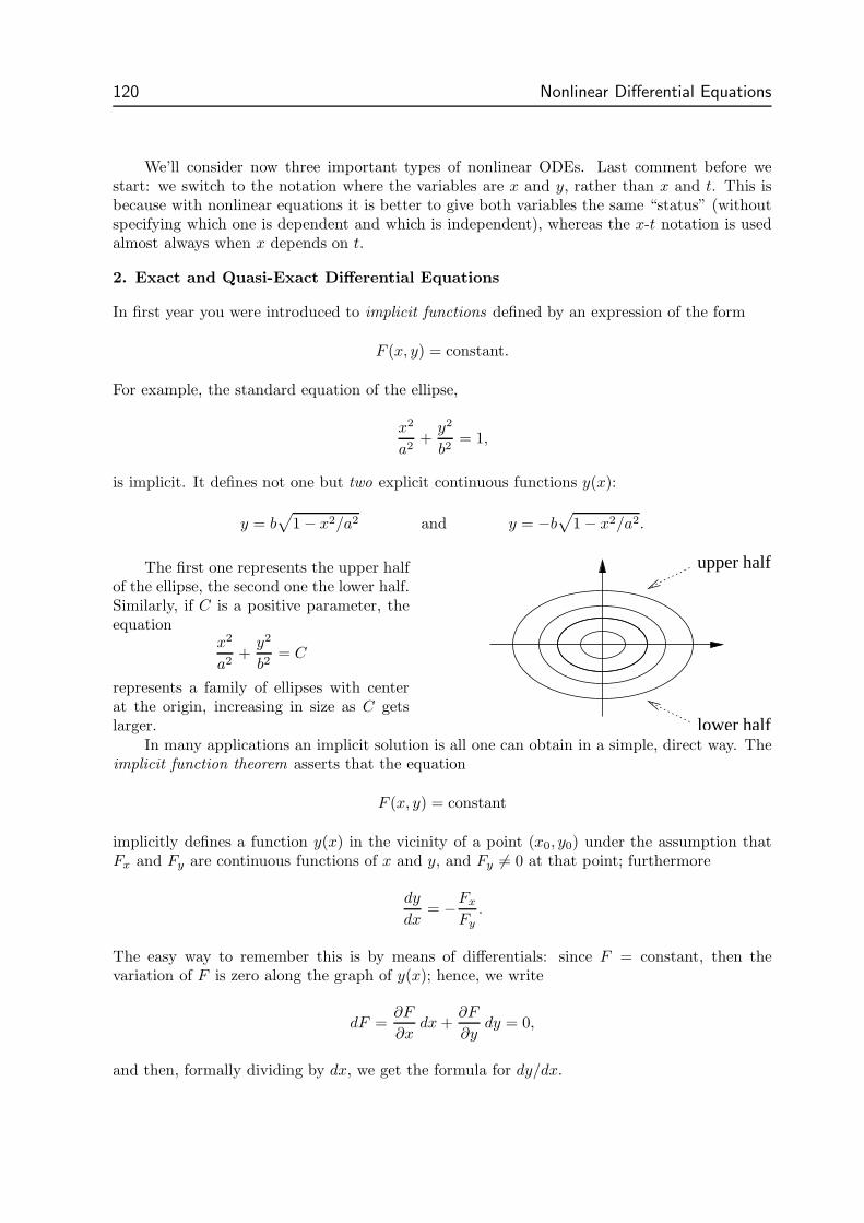
120 Nonlinear Differential Equations
We’ll consider now three important types of nonlinear ODEs. Last comment before westart: we switch to the notation where the variables are x and y, rather than x and t. This isbecause with nonlinear equations it is better to give both variables the same “status” (withoutspecifying which one is dependent and which is independent), whereas the x-t notation is usedalmost always when x depends on t.
2. Exact and Quasi-Exact Differential Equations
In first year you were introduced to implicit functions defined by an expression of the form
F (x, y) = constant.
For example, the standard equation of the ellipse,
x2
a2+
y2
b2= 1,
is implicit. It defines not one but two explicit continuous functions y(x):
y = b√
1 − x2/a2 and y = −b√
1 − x2/a2.
The first one represents the upper halfof the ellipse, the second one the lower half.Similarly, if C is a positive parameter, theequation
x2
a2+
y2
b2= C
represents a family of ellipses with centerat the origin, increasing in size as C getslarger.
upper half
lower halfIn many applications an implicit solution is all one can obtain in a simple, direct way. The
implicit function theorem asserts that the equation
F (x, y) = constant
implicitly defines a function y(x) in the vicinity of a point (x0, y0) under the assumption thatFx and Fy are continuous functions of x and y, and Fy 6= 0 at that point; furthermore
dy
dx= −Fx
Fy.
The easy way to remember this is by means of differentials: since F = constant, then thevariation of F is zero along the graph of y(x); hence, we write
dF =∂F
∂xdx +
∂F
∂ydy = 0,
and then, formally dividing by dx, we get the formula for dy/dx.
Nonlinear Differential Equations 121
Obviously x and y may be interchanged, and the corresponding result for x(y) is
dx
dy= −Fy
Fx,
with the assumption, now, that Fx 6= 0.These formulas may be interpreted backwards. Consider a differential equation of the form
P (x, y) + Q(x, y) y′(x) = 0 or P (x, y)x′(y) + Q(x, y) = 0;
we agree that either equation may also be written in the symmetric form
P (x, y) dx + Q(x, y) dy = 0, (50)
which is equivalent to both, wherever the assumptions of the implicit function theorem aresatisfied. Now suppose that there exists a function F (x, y) such that
∂F
∂x= P and
∂F
∂y= Q : (51)
then the formal manipulations
P dx + Qdy = 0 =⇒ ∂F
∂xdx +
∂F
∂ydy = 0 =⇒ dF = 0 =⇒ F = C
(where C = constant) yield the solution in implicit form.
Example 144 Find the solution of y′ + (4x3y2 − 2x)/2x4y = 0.
Solution: First of all, put this equation in the form (50):
(4x3y2 − 2x) dx + 2x4y dy = 0.
Then, note that
4x3y2 − 2x =∂(x4y2 − x2)
∂xand 2x4y =
∂(x4y2 − x2)
∂y;
conditions (51) are satisfied by the function F (x, y) = x4y2 −x2, hence the (implicit) solution is
x4y2 − x2 = C,
where C = constant. In this example one may go one step further, and write the explicitsolutions:
y = ±√
C + x2
x2,
but in general this last step may not be possible.
Definition: An equation of the form P dx + Qdy = 0 for which a function F (x, y) exists sothat conditions (51) are satisfied, is called exact.
122 Nonlinear Differential Equations
We note immediately that if an equation is exact, then by N. Bernoulli’s theorem† on mixedpartial derivatives, we have:
∂2F
∂x∂y=
∂2F
∂y ∂x=⇒ ∂P
∂y=
∂Q
∂x.
Hence, if the last condition is not satisfied, then there is no point in looking for a functionF satisfying conditions (51), because such a function cannot exist. So, the mixed-derivativescondition
∂P
∂y=
∂Q
∂x, (52)
is necessary for an equation of the form (50) to be exact.Moreover, if P and Q, besides satisfying (52), are also continuous, then it is not hard to
show that this condition is also sufficient: in other words, a function F exists such that (51)hold, and the equation is exact. Let’s see how this comes to work in practice.
Example 145 Check that the equation (2xyex2 − 2x) dx + (ex2
+ 3y2) dy = 0 is exact, andsolve it.
Solution: First of all, we check for exactness. Clearly P and Q are continuous, and
∂P
∂y=
∂
∂y
(
2xyex2 − 2x)
= 2xex2
,∂Q
∂x=
∂
∂x
(
ex2
+ 3y2)
= 2xex2
:
hence (52) holds, and the equation is exact. Now, to find F (x, y) we may proceed as follows.We note that
∂F
∂x= P = 2xyex2 − 2x;
integrating this equation with respect to x (i.e., treating y as a parameter) we get:
F (x, y) =
∫
(2xyex2 − 2x) dx = yex2 − x2 + “a constant”.
Careful now: “a constant” here means “any expression that does not depend on x”, becauseany function of y alone remains constant if only x is varied. So, we rewrite the last result as
F (x, y) = yex2 − x2 + g(y), (53)
where g(y) is a function of y alone. In this way, we’ve made sure that the first of conditions (51)is satisfied, but g is still undetermined. To find it, we require that the second of conditions (51),i.e., ∂F/∂y = Q, is also satisfied. It follows that
∂
∂y
(
yex2 − x2 + g(y))
= ex2
+ 3y2,
ex2
+ g′(y) = ex2
+ 3y2,
g′(y) = 3y2.
† Nicholas Bernoulli (1687-1759), a Swiss who lectured at Padua (Italy); not to be confusedwith his cousin Nicholas Bernoulli (1695-1726), who discovered the St. Petersburg paradox. TheBernoulli differential equation, which you saw in problems 42–43, is named after their uncleJakob Bernoulli (1654-1705).
Nonlinear Differential Equations 123
We see that the last equation does not contain x anymore. Hence, by a trivial integration withrespect to y, we get
g(y) + C = y3,
where C is a true constant. Combining our results, we finally get that
F (x, y) = yex2 − x2 + y3 = C,
and this is the general solution in implicit form.
As a rule, after one has established that a given equation is exact, there are several avenues forfinding F (x, y), all pretty much equivalent.
The procedure used in example 145 went through three steps: first, integrate P with respectto x, up to an unknown function g(y). Second, take the partial derivative of this integral withrespect to y, and compare the result with Q; the resulting equation must contain only y (if itdoesn’t, it’s a flag for a mistake in the calculations). Third, integrate g′(y) to find g(y).
Alternatively, one may integrate Q with respect to y, up to an unknown function g(x), andthen take the partial derivative of this integral with respect to x, comparing the result withP . The resulting equation must contain only x, and one may therefore find g(x) by integratingg′(x). This procedure is the “mirror image” of the first one.
One may also integrate P with respect to x, up to a function g(x), and then Q with respectto y, up to a function h(y). Comparing the two results, which must be equivalent, one determinesg(x) and h(y).
Example 146 Solve by comparison the equation of example 145.
Solution: Having already found with equation (53) that
F (x, y) = yex2 − x2 + g(y),
we integrate Q with respect to y; this yields:
F (x, y) =
∫
(ex2
+ 3y2) dy = yex2
+ y3 + h(x).
Comparing the two expressions above for F , we deduce that
h(x) = −x2 and g(y) = y3.
Therefore, F (x, y) = yex2 − x2 + y3, as expected.
Example 147 Check that the equation(
x√
x2 + y2 − x − y)
dx +(
y√
x2 + y2 − x)
dy = 0is exact and find the general solution.
Solution: Clearly P and Q are continuous, and
Py =∂
∂y
(
x√
x2 + y2 −x−y)
=xy
√
x2 + y2−1, Qx =
∂
∂x
(
y√
x2 + y2−x)
=xy
√
x2 + y2−1 :
hence the equation is exact. Integrating Q with respect to y, we find:
F (x, y) =
∫
(
y√
x2 + y2 − x)
dy = 13 (x2 + y2)3/2 − xy + g(x),
124 Nonlinear Differential Equations
where g(x) depends on x alone. Differentiating this result with respect to x, and comparing theresult with P , we get:
∂
∂x
[
13 (x2 + y2)3/2 − xy + g(x)
]
= x√
x2 + y2 − x − y
x√
x2 + y2 − y + g′(x) = x√
x2 + y2 − x − y
g′(x) = −x.
The last line contains x alone, hence by integration we find that
g(x) + C = − 12x2,
which finally yieldsF (x, y) = 1
3 (x2 + y2)3/2 − xy − 12x2 = C.
This is the general solution in implicit form.
Exact differential equations are closely connected to conservative vector fields. The link becomesclear if one considers a two-dimensional vector field f defined as
f = P ı + Q ,
where P = P (x, y) and Q = Q(x, y). Then we know that f is conservative if
∇× f = 0, i.e., (Qx − Py) k = 0;
the last condition is equivalent to (52). Furthermore, if f physically corresponds to a force, thenthe expression Pdx + Qdy represents the “infinitesimal” work done by f on a particle movingfrom (x, y) to (x + dx, y + dy); the solutions of equation (50)
P dx + Qdy = 0,
which are given byF (x, y) = C,
are curves along which f does no work. Finally: since f = P ı + Q = ∇F , then −F is thepotential energy associated with the force f .
INTEGRATING FACTORS
An unpleasant feature of exact equations is that if they are altered in an insignificant way, theymay lose their exactness. For example, consider the equation
y′ = y,
which has the general solution y = Cex. If written
dx − dy
y= 0
Nonlinear Differential Equations 125
it is exact, because P = 1, Q = −1/y, and Py = Qx = 0. But if written
y dx − dy = 0,
which is clearly equivalent, it is not exact because P = y, Q = −1, Py = 1, Qx = 0, andQx 6= Py : the mixed-derivatives condition (52) does not hold. What’s more disturbing, if onemultiplies through the equation above by y−1, which at first sight looks like a pointless move,
y−1 · (y dx − dy) = 0,
one obtains the exact equation again. This example is purely academic because the equationy′ = y is so easy that we can solve it by inspection; but the point is important.
It may be shown that any equation of the form (50) may, under reasonable assumptions,be made exact if it’s multiplied through by an appropriate function µ(x, y). Unfortunately, thesame theorem that guarantees the existence of µ does not say a word about how to find it.
Definition: A function µ(x, y) such that an equation of the form P dx + Qdy = 0 becomesexact if it is multiplied through by µ, is called an integrating factor for the equation.
Example 148 Show that µ(x, y) = x is an integrating factor for the equation (2y − 3x) dx +x dy = 0, and solve it.
Solution: The equation(2y − 3x) dx + x dy = 0
is not exact because Qx = 1 and Py = 2. However, if it’s multiplied through by x, one gets
(2xy − 3x2) dx + x2 dy = 0.
Now, Qx = 2x, Py = 2x, and the equation has become exact; hence µ = x is an integratingfactor. We proceed by integrating Q with respect to y:
F (x, y) = x2y + g(x),
where g is determined by the first of conditions (51):
Fx = 2xy + g′(x) = P = 2xy − 3x2.
It follows that g′(x) = −3x2, g(x) + C = −x3, and finally that F (x, y) = x2y − x3 = C. Notethat in this example one can write an explicit solution in the form y = C/x2 + x.
Example 149 Show that the equation (xy−2y2) dx+(3xy−x2) dy = 0 admits the integratingfactor µ(x, y) = 1/xy2; find the general solution.
Solution: The equation(xy − 2y2) dx + (3xy − x2) dy = 0
is not exact because Py = x − 4y and Qx = 3y − 2x. However, if it’s divided through by xy2,one gets
xy − 2y2
xy2dx +
3xy − x2
xy2dy = 0
(
1
y− 2
x
)
dx +
(
3
y− x
y2
)
dy = 0.
126 Nonlinear Differential Equations
Written in this form, the equation is exact because Py = −1/y2 and Qx = −1/y2. IntegratingP with respect to x, we get:
F (x, y) =
∫(
1
y− 2
x
)
dx =x
y− 2 ln |x| + g(y),
where g(y) is determined by the second of conditions (51). It follows that:
− x
y2+ g′(y) =
3
y− x
y2,
and hence that g′(y) = 3/y, g(y) + C = 3 ln |y|, and finally that
x
y− 2 ln |x| + 3 ln |y| = C.
Example 150 Show that the equation (x2 + 2x + y) dx + (1 − x2 − y) dy = 0 admits theintegrating factor µ(x, y) = ex−y; find the general solution.
Solution: The equation(x2 + 2x + y) dx + (1 − x2 − y) dy = 0
is not exact because Py = 1 and Qx = −2x. However, if it’s multiplied through by ex−y, onegets
ex−y · (x2 + 2x + y) dx + ex−y · (1 − x2 − y) dy = 0;
now, by the product rule, we obtain:
Py = −ex−y · (x2 + 2x + y) + ex−y · 1 = ex−y · (1 − x2 − 2x − y)
Qx = ex−y · (1 − x2 − y) + ex−y · (−2x) = ex−y · (1 − x2 − 2x − y)
and the equation is exact. Integrating (by parts) Q with respect to y, we get that
F (x, y) = ex−y · (y + x2) + g(x),
where g is determined by the first of (51):
Fx = ex−y · (y + x2) + ex−y · 2x + g′(x) = ex−y · (x2 + 2x + y).
It follows that g′(x) = 0, g = C, and finally that ex−y · (y + x2) = C.
Example 151 The first principle of thermodynamics says that if heat enters a system at arate Q, then
Q = U + W ,
where U is the rate at which the internal energy increases, and W is the rate at which the systemis doing work. (These quantities have the same dimensions as power, so they could be measuredin Watt.) Integrating with respect to time, we get
∆Q = ∆U + ∆W,
Nonlinear Differential Equations 127
which is an equivalent (and perhaps more familiar) statement of the first principle. The disad-vantage of this notation is that, since the time interval of integration may be made arbitrarilysmall, one is tempted to write
dQ?= dU + dW.
But this is wrong, because dQ is not an exact differential. There is no guarantee that there is astate function Q such that its differential is equal to dU + dW .
It may be shown, however, that an integrating factor for dQ always exists, and that it isequal to 1/T . This, in turn, means that the path integral
S =
∫(
dU
T+
dW
T
)
(54)
depends only on the initial and final states of the system, and not on the type of transformation(such as adiabatic, isobaric, isothermal, etc) that connects them—as long as it is a reversibletransformation, obviously.
For example, consider an ideal gas: you have probably seen in your physics courses thatthe internal energy of an ideal gas is U = CV T , where T is the absolute temperature, and CV
is a constant. You also know that the work done by an expanding gas is W =∫
p dV , where pand V are pressure and volume, respectively. Substituting back, we get
dQ?= CV dT + p dV ;
but remember that p depends on T and V through the equation of state which, for an ideal gas,is p = nRT/V . It follows that
dQ?= CV dT +
nRT
VdV,
and we see immediately that the right-hand side is not exact: from the exactness condition (52),we get
∂CV
∂V= 0,
∂
∂T
(
nRT
V
)
=nR
V,
and the two are not equal. Hence, there is no function Q(T, V ) such that (∂Q/∂T )V = CV and(∂Q/∂V )T = nRT/V .
If however we multiply dQ by the integrating factor 1/T and then integrate, we get (54),which for an ideal gas becomes
S =
∫(
CV
TdT +
nRT
V TdV
)
= CV ln T + nR ln V + constant,
where(
∂S
∂T
)
V
=CV
T,
(
∂S
∂V
)
T
=nR
V.
The exactness condition (52) holds because both ∂2S/∂V ∂T and ∂2S/∂T ∂V are = 0.The principle of existence of the integrating factor 1/T is mathematically equivalent to
the second principle of thermodynamics. However, the proof of this fairly advanced concept(Caratheodory’s principle) is beyond the scope of these notes; interested students can find a briefdescription in H. Margenau and G.M. Murphy, The Mathematics for Physics and Chemistry,Krieger (USA) 1976.
128 Nonlinear Differential Equations
QUASI-EXACT EQUATIONS
If you thought that there was practically no way of guessing the integrating factors in the lastexamples, you have a point. As we saw, the theorem that asserts the existence of integratingfactors does not provide any method for finding them; for a generic differential equation of theform (50) we have to live with that.
There are exceptions, though. Among them, we’ll consider only the class of “quasi-exact”equations: these are equations that admit an integrating factor that depends on one variableonly, but not on the other. For quasi-exact equations there is a simple procedure for finding µ.
Suppose—for the sake of the argument—that the integrating factor for the equation (50)depend on x alone, i.e., assume that µ = µ(x). In other words, assume the equation
µ(x)P (x, y) dx + µ(x)Q(x, y) dy = 0
is exact. Then,by the product rule, (52) yields:
∂(µ P )
∂y=
∂(µ Q)
∂x
µ Py = µ′ Q + µ Qx,
where µ′ = dµ/dx. Simple manipulations lead to the equation
µ′
µ=
Py − Qx
Q.
Recall, we assumed that µ depends only on x; hence, the left-hand side above depends on xalone. Therefore, if the right-hand side depends on x and y, the method fails. If, however,(Py − Qx)/Q depends on x alone, then we may find µ by integration:
ln |µ(x)| =
∫
Py − Qx
Qdx.
Make sure you understand this point: the integration of the right-hand side is meaningfulonly if (Py − Qx)/Q depends on x alone.
In exactly the same way, one may see that if (Qx−Py)/P depends on y alone, then an integratingfactor is given by the equation
ln |µ(y)| =
∫
Qx − Py
Pdy.
In summary, an equation is quasi-exact if either (Py−Qx)/Q depends on x alone, or (Qx−Py)/Pdepends on y alone. In the first case, µ = µ(x), and in the second case µ = µ(y).
Example 152 Find the integrating factor of example 148.
Solution: The equation (2y − 3x) dx + x dy = 0 is quasi-exact because
Py − Qx
Q=
2 − 1
x
depends only on x. Hence, the integrating factor is given by
ln |µ| =
∫
dx
x= ln |x| + C,
Nonlinear Differential Equations 129
which yields µ = x, as expected (the integration constant is irrelevant).
You should convince yourself that the integration constant arising in the calculation of µ mayalways be set equal to zero without loss of generality. Therefore, for the rest of this section we’llignore it.
Example 153 Find an integrating factor of the equation (x−y2) dx+2xy dy = 0, and solve it.
Solution: The equation is quasi-exact because
Py − Qx
Q=
−2y − 2y
2xy= − 2
x;
therefore
ln |µ| = −2
∫
dx
x= ln x−2.
An integrating factor is µ = x−2; dividing the original equation by x2, we get:
(
1
x− y2
x2
)
dx +2y
xdy = 0,
which is exact. Integrating Q with respect to y, we find that
F (x, y) =
∫
2y
xdy =
y2
x+ g(x),
where g(x) is determined by the first of conditions (51):
Fx = −y2
x2+ g′(x) =
1
x− y2
x2.
It follows that g′(x) = 1/x, g(x)+ C = ln |x|, and finally y2/x+ ln |x| = C, which is the generalsolution.
Example 154 Find an integrating factor of the equation (2y +3y2ex) dx+(1+2yex) dy = 0,and solve it.
Solution: The equation is quasi-exact because
Py − Qx
Q=
2 + 6yex − 2yex
1 + 2yex= 2;
therefore
ln |µ| =
∫
2 dx = 2x.
An integrating factor is µ = e2x; multiplying the original equation by e2x we get:
(2ye2x + 3y2e3x) dx + (e2x + 2ye3x) dy = 0,
which is exact. Integrating P with respect to x we find that:
F (x, y) =
∫
(2ye2x + 3y2e3x) dx = ye2x + y2e3x + g(y),
130 Nonlinear Differential Equations
where g(y) is determined by the second of conditions (51):
Fy = e2x + 2ye3x + g′(y) = e2x + 2ye3x.
It follows that g′(y) = 0, g(y) = C, and finally that e2x + 2ye3x = C, which is the generalsolution. This one may be made explicit: y = 1
2Ce−3x − 12e−x.
Example 155 Find an integrating factor of the equation y dx − (x + 1 − y2) dy = 0, andsolve it.
Solution: We note immediately that
Py − Qx = 1 − (−1) = 2;
unfortunatelyPy − Qx
Q=
2
−(x + 1 − y2),
which certainly is not a function of x alone. However, observe that P = y: therefore,
Qx − Py
P=
−2
y
is a function of y alone. Therefore, there is an integrating factor of the form µ = µ(y), given bythe equation
µ′(y)
µ(y)= −2
y.
A simple integration yields ln |µ| = ln |y|−2, i.e., µ = y−2. Dividing the original equation by y2,we get:
dx
y−
(
x
y2+
1
y2− 1
)
dy = 0,
which is exact. Integrating P with respect to x we find that
F (x, y) =x
y+ g(y).
Integrating Q with respect to y we find that
F (x, y) =x
y+
1
y+ y + h(x).
By comparison, we see that
g(y) =1
y+ y and h(x) = 0;
hencex
y+
1
y+ y = C
is the general solution. In explicit form, this may be written x = Cy − y2 − 1.
Nonlinear Differential Equations 131
3. Scale-Invariant Equations
If an equation retains the same form when x and y are scaled by the same amount, it is calledscale-invariant. A first-order scale-invariant equation is easy to recognize when it’s written inthe form
y′ = f(y/x),
where f(y/x) is some function of the ratio y/x.It is rather unfortunate that most books call these equations “homogeneous”, a choice that
can be confusing for a beginner since they have nothing to do with the homogeneous equationswe met in chapter 3. The name “scale-invariant” has been suggested, among others, by Benderand Orszag.†
If a first-order equation is scale-invariant, then either of the substitutions
u =y
xor u =
x
y
will transform it into a separable equation.
Example 156 Show that the differential equation (2xy−y2) dx−x2 dy = 0 is scale-invariant,and solve it.
Solution: If one introduces the scaled variables
x = aX y = aY,
then the equation becomes
a2(2XY − Y 2) a dX − a2X2a dY = 0,
which (after canceling the common factor a3) has the same form as the original. Note also thatthe equation may be written as
dy
dx=
2xy − y2
x2=
2(y/x) − (y/x)2
1,
which shows immediately the scale-invariance property.
Method 1: Substitute
u =y
x=⇒ y = xu, y′ = u + xu′,
where u = u(x) is the new unknown. It follows that
u + xu′ = 2u − u2
du
u(1 − u)=
dx
x∫
(
1
u− 1
u − 1
)
du =
∫
dx
x;
† Advanced Mathematical Methods for Scientists and Engineers, McGraw-Hill (1978).
132 Nonlinear Differential Equations
integrating, we get that
ln∣
∣
∣
u
u − 1
∣
∣
∣= ln |x| + C,
y/x
y/x − 1= Bx,
where B = ±eC is a new constant replacing C, and finally that y = Bx(y − x).
Method 2: Substitute
u =x
y=⇒ x = yu, x′ = u + yu′,
where u = u(y) is the new unknown. It follows that
dx
dy=
(x/y)2
2(x/y) − 1
u + yu′ =u2
2u − 1.
From here onwards, follow the steps of method 1 (separate the variables, use partial fractions,integrate with respect to y). Do it, as an exercise.
You may also observe that the original equation becomes a Bernoulli equation if formallydivided by dx: x dy/dx − 2y = −y2/x. See problem 42.
Example 157 Solve the equation xy′ = y +√
x2 + y2.
Solution: That the equation is scale-invariant is evident when it’s rewritten as follows:
y′ =y +
√
x2 + y2
x=
y
x+
√
1 +y2
x2.
Substituting y = xu, y′ = u + xu′, one gets immediately:
u + xu′ = u +√
1 + u2,
du√1 + u2
=dx
x.
Hence, after integration:arsinhu = ln |x| + C,
earsinh u = Bx,
where B = ±eC is a new constant replacing C. Using the trivial identities
earsinh u = cosh(arsinh u) + sinh(arsinhu) =√
1 + u2 + u,
one finally gets:√
1 + y2/x2 + y/x = Bx,√
x2 + y2 + y = Bx2.
Example 158 Solve the equation xy′ = y(ln y − ln x).
Nonlinear Differential Equations 133
Solution: Rewriting the equation as
y′ = (y/x) ln(y/x)
(note the scale-invariance) and substituting y = xu, y′ = u + xu′, one gets immediately:
u + xu′ = u ln u.
Hence,xu′ = u (ln u − 1)
du
u (ln u − 1)=
dx
x.
Integrating, we get:∫
du
u (ln u − 1)= ln
∣
∣ ln u − 1∣
∣ = ln |x| + C,
and then (introducing a new constant B that may take negative values):
ln u − 1 = Bx.
It follows that ln(y/x) = 1 + Bx, and finally that y = xe1+Bx.
4. Autonomous Equations
An equation is called autonomous if the independent variable is missing. If the equation is ofsecond order, the substitution p = dy/dx, combined with the chain rule, transforms it into afirst-order equation where p(y) is the unknown:
dy
dx= p =⇒ d2y
dx2=
dp
dx=
dp
dy
dy
dx=
dp
dy· p. (55)
The best-known autonomous equation is almost certainly the simple harmonic motion equation:x + ω2x = 0, or (with the notation of this chapter) y′′ + ω2y = 0.
Example 159 Solve the harmonic motion equation without using the methods of chapter 3.
Solution: Following (55), we let y′ = p and hence y′′ = p dp/dy. It follows:
pdp
dy= −ω2y,
∫
p dp = −ω2
∫
y dy.
A simple integration yields: 12p2 = C − 1
2ω2y2. Defining a new constant A through the equationC = 1
2ω2A2, we get
p =dy
dx= ±|ω|
√
A2 − y2
∫
dy√
A2 − y2= ω
∫
dx;
in the last step, ω is allowed negative values. Another simple integration gives
− arccos y/A = ωx + Φ
(where Φ = constant), which finally yields the classic solution y = A cos(ωx + Φ).
Example 160 Solve the autonomous equation y3y′′ = 1.
Solution: By means of the substitution (55), we get:
134 Nonlinear Differential Equations
y3pdp
dy= 1,
∫
p dp =
∫
y−3 dy.
Integrating, we obtain:12p2 = − 1
2y−2 + C = − 1
2y−2 + 1
2a2,
where a is a constant replacing C. It follows that
p =dy
dx=
√
a2 − y−2
±∫
y dy√
a2y2 − 1=
∫
dx.
Integrating again, we get that
±√
a2y2 − 1 = a2x + b,
where b is another constant, and finally that a2y2 − 1 = (a2x + b)2.
Example 161 Solve the autonomous equation y y′′ = y′2 + y2.
Solution: By (55), we get:
ypdp
dy= p2 + y2.
This is a scale-invariant equation. Proceeding along the lines of examples 157–158 (but bearingin mind that the variables are now p and y), we first rewrite the last equation as follows:
dp
dy=
p
y+
y
p(56)
(which shows the scale invariance). We then introduce a new variable u:
p = uy =⇒ dp
dy=
du
dyy + u,
and substitute back into (56):du
dyy + u = u +
1
u.
Simplifying, we get:
u du =dy
y12u2 = ln |y| + C
|u| =√
2 ln |y| + 2C
±p
y=
√
2 ln |y| + 2C.
But p = dy/dx; substituting back and rearranging, we get:
±∫
dy
y√
2 ln |y| + 2C=
∫
dx.
Nonlinear Differential Equations 135
Integration is trivial; it follows that
±√
2 ln |y| + 2C = x + B,
and hence that2 ln |y| + 2C = (x + B)2 =
= x2 + 2Bx + B2.
An explicit solution is obtained as follows:
ln |y| = 12x2 + Bx + 1
2B2 − C,
y = ± exp(12x2 + Bx + 1
2B2 − C),
y = A exp(12x2 + Bx)
where A = ± exp(12B2 − C) is a new (possibly negative) constant.
Example 162 Solve the differential equation
(1 + y2)y′′ − yy′2 = 0.
Solution: Substitution (55) gives:
(1 + y2)pdp
dy= yp2.
Therefore, either p = 0, hence y′ = 0, y = constant; or, dividing through by p, it follows:
(1 + y2)dp
dy= yp.
Separating the variables, one gets:dp
p=
y dy
1 + y2.
A straightforward integration yields:
ln |p| = 12
ln |1 + y2| + C,
hence
p =dy
dx= ±
√
1 + y2 · eC .
Defining A = ±eC , and separating again the variables, one finds that
dy√
1 + y2= Adx.
One more integration finally yields:
arsinh y = Ax + B,
which may also be written y = sinh(Ax + B). Note that the explicit solution of this equationcan be written both in the form x = x(y) and y = y(x).
136 Tutorial Problems Nonlinear Differential Equations
PROBLEMS
Exact ODEs
61. Check that the following ODEs are exact and hence find the general solution.
(a) (3e3xy − 2x) dx + e3xdy = 0
(b) (6x5y3 + 4y5x3 + 21x2) dx + (3x6y2 + 5x4y4 − 10y) dy = 0
(c) (cos x + cos y) dx − x sin y dy = 0
(d) (1 + yexy) dx + (2y + xexy) dy = 0
Integrating Factors
62. Solve the following equations, using the suggested integrating factors.
(a) (3y + 4xy2) dx + (2x + 3x2y) dy = 0, µ = x2y
(b) y dx + x(1 + 3x2y2) dy = 0, µ = 1/(xy)3
(c) y dx − (y5 + y3x2 + x) dy = 0, µ = 1/(x2 + y2)
63. Show that the first order linear equation c1(t) dy + c0(t) y dt = f(t) dt
[go back to (40) in section 3.6] admits the integrating factor
µ(t) =exp
∫
(c0/c1) dt
c1.
Many books present this as the “best” method for solving first order linear ODEs.
Quasi-Exact Equations
64. The following equations admit an integrating factor that depends on x alone or y alone.
Find it, and hence solve the equation.
(a) (x2 − xy + y3 + 2x − y) dx + (3y2 − x) dy = 0
(b) (x4 + y4) dx − xy3 dy = 0
(c) 7xy dx + (x2 + y2 + y) dy = 0
(d) (y + ey−x) dx + (1 + xey−x) dy = 0
Scale Invariant Equations
65. Find the general solution of the following equations.
(a) xy′ = y − x sin(y/x)
(b) xy y′ =√
x4 + y4 + y2
(c) y = (x + ye−x/y) y′
(d) (xy + y2) dx − (xy − x2) dy = 0
(e) y2 dx + (x2 − xy − y2) dy = 0
(f) 4y′ = (x/y)3 + 5(y/x)
(g) xy − x2 cos(y/x) = y2/y′
Nonlinear Differential Equations Tutorial Problems 137
Autonomous Equations
66. Find the general solution of the following equations.(a) y2y′′ = y′3
(b) yy′′ + y′2 = yy′2
(c) y′′ = 1/√
y
(d) y′′ = y′2 tan y
(e) y′′ = (ey − 1)y′2
(f) y′′ = y−3 − y
ANSWERS
61 (a) e3xy − x2 = C(b) x6y3 + x4y5 + 7x3 − 5y2 = C(c) x cos y + sin x = C(d) x + y2 + exy = C
62 (a) x3y2 + x4x3 = C(b) 3 ln |y| − 1/2x2y2 = C(c) arctan(y/x) − 1
4y4 = C
64 (a) µ = 1/x3, F (x, y) = ex(x2 − xy + y3) = C;(b) µ = 1/x5, F (x, y) = ln |x| − y4/4x4 = C;(c) µ = y−5/7, F (x, y) = 7
2xy2/7 + 716y16/7 + 7
9y9/7 = C;(d) µ = ex, F (x, y) = yex + xey = C.
65 (a) cos y/x = 1 − 2/(Bx2 + 1), where B > 0.(b) B2x4 = 2By2 + 1, where B > 0.(c) x = y ln
(
ln |y| + C)
.
(d) xy = Cey/x.(e) (x − y)y2 = C(x + y).(f) y = 4
√
|Ax5 − x4|.(g) sin(y/x) = (A2y2 − 1)/(A2y2 + 1).
66 (a) x = B + Cy + ln |y|.(b) y + 1 = (Ax + B)ey.
(c) x = B + 23
(√y + C
)3/2 − 2C(√
y + C)1/2
.(d) sin y + B = Cx.(e) − exp(−ey) = Ax + B.(f) y2 = A2 ±
√A4 − 1 sin(2x + B), where |A| ≥ 1.