Landscape‐scale fuel treatment and wildfire … · Landscape-scale fuel treatment and...

Landscape-scale fuel treatment and wildfire impacts on carbonstocks and fire hazard in California spotted owl habitat

LINDSAYA. CHIONO,1,5,� DANNY L. FRY,1 BRANDON M. COLLINS,2,3

ANDREA H. CHATFIELD,4 AND SCOTT L. STEPHENS1

1Ecosystem Sciences Division, Department of Environmental Science, Policy, and Management,University of California, Berkeley, 130 Mulford Hall, Berkeley, California 94720 USA

2USDA Forest Service, Pacific Southwest Research Station, Davis, California 95618 USA3Center for Fire Research and Outreach, University of California, Berkeley, Berkeley, California 94720 USA

4Western EcoSystems Technology, Inc., 456 SWMonroe Ave, Suite 106, Corvallis, Oregon 97333 USA

Citation: Chiono, L. A., D. L. Fry, B. M. Collins, A. H. Chatfield, and S. L. Stephens. 2017. Landscape-scale fuel treatmentand wildfire impacts on carbon stocks and fire hazard in California spotted owl habitat. Ecosphere 8(1):e01648.10.1002/ecs2.1648

Abstract. Forest managers are challenged with meeting numerous demands that often include wildlifehabitat and carbon (C) sequestration. We used a probabilistic framework of wildfire occurrence to (1) esti-mate the potential for fuel treatments to reduce fire risk and hazard across the landscape and within pro-tected California spotted owl (Strix occidentalis occidentalis) habitat and (2) evaluate the consequences oftreatments with respect to terrestrial C stocks and burning emissions. Silvicultural and prescribed fire treat-ments were simulated on 20% of a northern Sierra Nevada landscape in three treatment scenarios that var-ied in the land area eligible for treatment. Treatment prescriptions varied with topography, vegetationcharacteristics, and ownership. We then simulated many wildfires in the treated and untreated landscapes.Additional simulations allowed us to consider the influence of wildfire size on estimated emissions. Treat-ments constrained to the land area outside of spotted owl activity centers reduced the probability of burn-ing and potential fire intensity within owl habitat and across the landscape relative to no-treatmentscenarios. Allowing treatment of the activity centers achieved even greater fire hazard reductions withinthe activity centers. Treatments also reduced estimated wildfire emissions of C by 45–61%. However, emis-sions from prescribed burning exceeded simulated reductions in wildfire emissions. Consequently, alltreatment scenarios resulted in higher C emissions than the no-treatment scenarios. Further, for wildfiresof moderate size (714–2133 ha), the treatment scenarios reduced the C contained in live tree biomass fol-lowing simulated wildfire. When large wildfires (8070–10,757 ha) were simulated, however, the treatmentscenario retained more live tree C than the no-treatment scenario. Our approach, which estimated terres-trial C immediately following wildfire, did not account for long-term C dynamics, such as emissions asso-ciated with post-wildfire decay, C sequestration by future forest growth, or longer-term C sequestration instructural wood products. While simulated landscape fuel treatments in the present study reduced the riskof uncharacteristically severe wildfire across the landscape and within protected habitat, the C costs oftreatment generally exceeded the C benefits.

Key words: ArcFuels; California spotted owl; forest thinning; prescribed fire; Strix occidentalis occidentalis; wildfireemissions.

Received 31 October 2016; accepted 2 November 2016. Corresponding Editor: Debra P. C. Peters.Copyright: © 2017 Chiono et al. This is an open access article under the terms of the Creative Commons AttributionLicense, which permits use, distribution and reproduction in any medium, provided the original work is properly cited.5 Present address: Department of Natural Resources, Confederated Tribes of the Umatilla Indian Reservation, 46411Tim�ıne Way, Pendleton, Oregon 97801 USA.� E-mail: [email protected]

❖ www.esajournals.org 1 January 2017 ❖ Volume 8(1) ❖ Article e01648

info:doi/10.1002/ecs2.1648

http://creativecommons.org/licenses/by/3.0/

INTRODUCTION

Forest managers in fire-prone ecosystems seekto balance a complex set of sometimes competingobjectives that include providing wildlife habitat,avoiding catastrophic disturbance, and support-ing local economies. In recent years, maintainingand increasing the capacity of forests to store car-bon (C) has been added to these considerationsdue to concern over the effects of rising atmo-spheric greenhouse gas concentrations on theearth’s climate. In dry forests across much of thewestern United States, meeting these objectives iscomplicated by the increasing area and severityof wildfires occurring in concert with climatechange (McKenzie et al. 2004, Stephens 2005,Westerling et al. 2006, Miller et al. 2009).

A high-visibility example of competing objec-tives in forest management is spotted owl (Strixoccidentalis occidentalis) conservation in California.The northern (S. occidentalis caurina) and Mexican(S. occidentalis lucida) spotted owl subspecies havebeen listed as Threatened under the EndangeredSpecies Act. Management directives for the Cali-fornia subspecies focus on conserving nesting androosting habitat by identifying protected activitycenters (PACs): sites that include 121 ha (300 ac)of the best-quality habitat near known nest sites(Verner et al. 1992). Given the multi-storied, densecanopy forest characteristics of nesting and roost-ing sites, the potential vulnerability of PACs tohigh-severity fire is a challenge to owl conserva-tion (Collins et al. 2010, Stephens et al. 2016b).While low- to moderate-severity wildfire withinnesting and roosting habitat may not negativelyimpact owls in the short term (Bond et al. 2002),longer-term effects of high-severity wildfire caninclude significant habitat loss due to direct andindirect tree mortality (Gaines et al. 1997, Joneset al. 2016, Stephens et al. 2016b). However, due touncertainty concerning the effects of fuels reduc-tion activities, management options for reducingwildfire hazard within PACs are restricted to lightprescribed burning, although some thinning ispermitted in the wildland–urban interface (USDAForest Service 2004).

There is concern that such constraints on man-agement activities limit the effectiveness of land-scape-scale treatments intended to reduce thethreat of uncharacteristically severe wildfire (Col-lins et al. 2010, Tempel et al. 2015). Fire modeling

studies have shown that treating a portion of thelandscape can alter simulated fire behavior withinand outside of treated areas and that strategicallylocating fuel treatments across the landscape hasthe potential to maximize treatment benefitswhile minimizing area treated (Finney et al. 2007,Schmidt et al. 2008). Restrictions on fuel treat-ment location and severity limit real-world appli-cation of treatment optimization methods. Evenso, there may be significant opportunity for activemanagement outside of high-quality owl habitaton fire-prone landscapes (Ager et al. 2007,Prather et al. 2008, Gaines et al. 2010).Given their demonstrated ability to alter wild-

fire behavior and effects (Martinson andOmi 2002,Pollet and Omi 2002, Ritchie et al. 2007, Ful�e et al.2012), fuel treatments that address accumulatedfuels and reduce stand density (e.g., prescribedburning, forest thinning, mastication) are com-monly applied in dry western forests where wild-fires were once frequent. It is less certain howtreatments influence C stocks, and how to maxi-mize C storage in frequent-fire systems. In theabsence of disturbance, untreated forests maysequester the most C (Hurteau and North 2009,Stephens et al. 2009, Hurteau et al. 2011). How-ever, high-severity wildfires can rapidly convert Csinks to sources, and burned forests may continueto be C sources for decades (Dore et al. 2008, 2012).Treatments can reduce wildfire emissions (Finkraland Evans 2008, Hurteau and North 2009, 2010,North et al. 2009a, Reinhardt and Holsinger 2010,Wiedinmyer and Hurteau 2010, North and Hur-teau 2011) andmay retainmore live tree C post fire(Hurteau and North 2009, North and Hurteau2011, Stephens et al. 2012). Yet fuel treatments areassociated with significant C emissions, releasingC to the atmosphere during harvest operations,burning, and/or biomass transport, and the C costof treating forest fuels may exceed its C benefits(Campbell et al. 2011, Campbell and Ager 2013).The circumstances under which treatments mightlead to a net gain in C have not yet been resolved.Recently, as a result of concern over the C costs

of fossil fuel use and the threat of wildfire, inter-est in harvesting historically low-value woodybiomass has increased (Evans and Finkral2009). Utilizing forest biomass for energy pro-duction can help to reduce the cost of fuel treat-ments, support local economies, offset fossil fueluse, and reduce the C and smoke emissions


CHIONO ET AL.

associated with fuel treatments (Reinhardt et al.2008). Concerns remain over the sustainability ofbiomass removals, funding, and the availabilityof markets (Evans and Finkral 2009).

The focus of our research was to (1) evaluatewhether withholding some land area from treat-ment influences potential wildfire hazard acrossthe landscape and within California spotted owlhabitat, (2) estimate the short-term C conse-quences of treatments, and (3) quantify the bio-mass harvested in treatments. We simulated fuelsreduction treatments and wildfire in a northernSierra Nevada study area that encompassed 61spotted owl PACs. In order to evaluate the C bal-ance of the treatment scenarios, we quantified theC contained in the forest biomass harvested ineach treatment scenario, the C emitted duringprescribed fire and wildfires, and the C remainingwithin onsite pools. We confined our analysis tothe immediate changes in C stocks and emissions,but recognize that a full accounting of treatmenteffects would also include long-term C dynamics(e.g., Dore et al. 2008, Malmsheimer et al. 2011).

METHODS

Study areaThe study area was defined by a long-

term demographic study site for the California

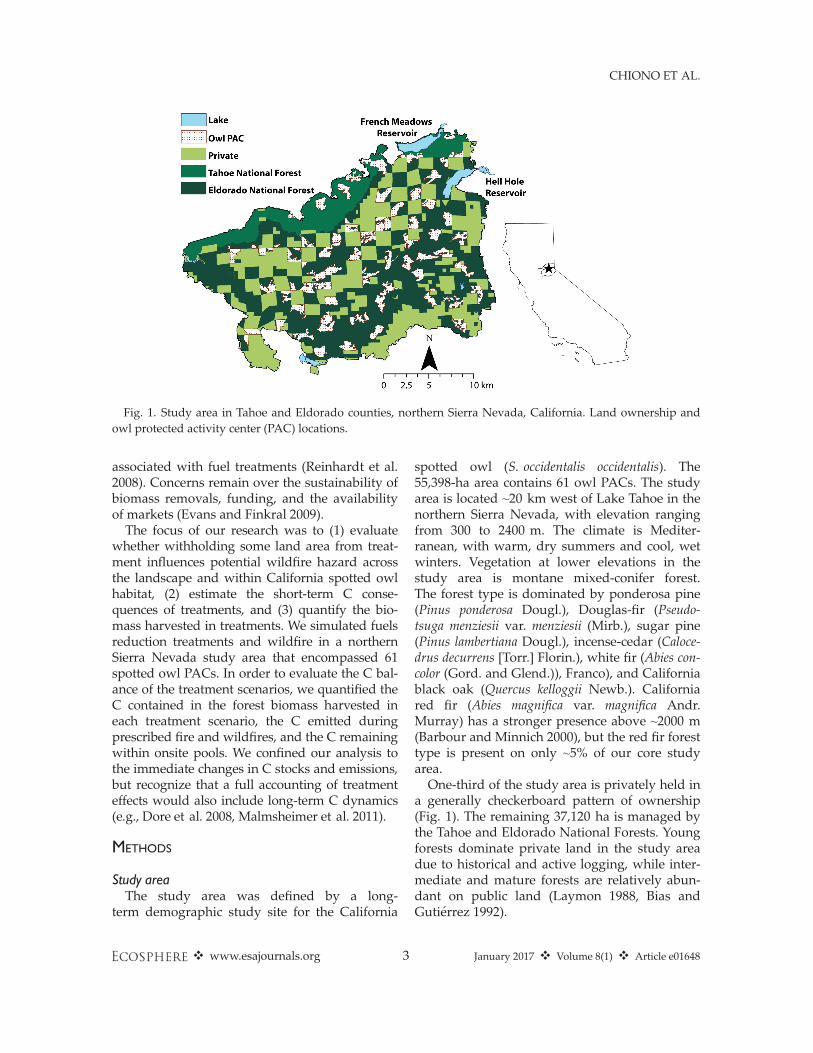
spotted owl (S. occidentalis occidentalis). The55,398-ha area contains 61 owl PACs. The studyarea is located ~20 km west of Lake Tahoe in thenorthern Sierra Nevada, with elevation rangingfrom 300 to 2400 m. The climate is Mediter-ranean, with warm, dry summers and cool, wetwinters. Vegetation at lower elevations in thestudy area is montane mixed-conifer forest.The forest type is dominated by ponderosa pine(Pinus ponderosa Dougl.), Douglas-fir (Pseudo-tsuga menziesii var. menziesii (Mirb.), sugar pine(Pinus lambertiana Dougl.), incense-cedar (Caloce-drus decurrens [Torr.] Florin.), white fir (Abies con-color (Gord. and Glend.)), Franco), and Californiablack oak (Quercus kelloggii Newb.). Californiared fir (Abies magnifica var. magnifica Andr.Murray) has a stronger presence above ~2000 m(Barbour and Minnich 2000), but the red fir foresttype is present on only ~5% of our core studyarea.One-third of the study area is privately held in

a generally checkerboard pattern of ownership(Fig. 1). The remaining 37,120 ha is managed bythe Tahoe and Eldorado National Forests. Youngforests dominate private land in the study areadue to historical and active logging, while inter-mediate and mature forests are relatively abun-dant on public land (Laymon 1988, Bias andGuti�errez 1992).

Fig. 1. Study area in Tahoe and Eldorado counties, northern Sierra Nevada, California. Land ownership andowl protected activity center (PAC) locations.


CHIONO ET AL.

Vegetation and fuels dataThe vegetation classification map developed in

Chatfield (2005) forms the basis of our study area.Using aerial photographs combined with fieldaccuracy assessment, Chatfield (2005) digitizedeight land cover classes consistent with theCalifornia Wildlife Habitat Relationships (CWHR;Mayer and Laudenslayer 1988) system. A descrip-tion of the cover classes is provided in Table 1.From the resulting cover class map, we delin-eated polygons to represent stands of similarvegetation composition and structure (n = 4470)based on aerial photographs and topography(Fig. 2).

Stands were populated with vegetation datacollected in 2007 in 382 sampling plots locatedwithin 10 km of the study area’s northern bound-ary, based on the assumption that the characteris-tics of the plots are representative of the studyarea. These vegetation data included tree species,heights, diameters, and crown ratios. See Collinset al. (2011) for a detailed description of data col-lection. To populate stands in the core study areawith plot data, we first assigned a Chatfield coverclass to each sampling plot based on species com-position, canopy cover, and tree diameter distri-bution. We then used a Most Similar Neighborprocedure (Crookston et al. 2002) to select fivenearest neighbor plots for each stand using theRandom Forest method with the R package yaim-pute (version 1.0-22; Crookston and Finley 2008).Variables used in identifying nearest neighborswere topographic relative moisture index, east-ness, northness, slope, and elevation. Stands were

populated with data only from plots belonging tothe same cover class. In order to increase variabil-ity in stand conditions, three of the five plots ini-tially selected to represent each stand werechosen randomly to contribute data to the stand.Each plot contributed data to an average of 35.5stands (range: 1–437).The method in which surface fuels are repre-

sented for fire modeling has important implica-tions for findings related to expected firebehavior and effects. Fuel models are representa-tions of fuelbed properties such as the distribu-tion of fuel between particle size classes, heatcontent, and dead fuel moisture of extinction foruse in the Rothermel (1972) surface fire spreadmodel. As representations, fuel models artifi-cially constrain the variation in surface fuelconditions. In order to represent a range of pre-treatment fuel conditions for fire modeling, weoverrode fuel model assignments made by theFire and Fuels Extension to the Forest VegetationSimulator (FVS-FFE, Dixon 2002, Reinhardt andCrookston 2003) and selected two fuel models foreach stand. Fuel models representing the lowend of the range were assigned following theselection logic of Collins et al. (2011); high-endmodels were selected to amplify surface firebehavior relative to the low-end models (App-endix S1: Table S1; Collins et al. 2013). Thisapproach to assigning fuel models to stands hasbeen demonstrated to result in modeled firebehavior that is more consistent with observedfire effects than default fuel model assignments(Collins et al. 2013). An alternative approachcould be to use the Landfire surface fuel modellayer (e.g., Scott et al. 2016). However, we optedto tie fuel model assignments to the specific foreststructural characteristics for each stand (Lydersenet al. 2015) as represented by the imputed plotsrather than the remotely sensed dominant vege-tation characteristics captured by Landfire.Study area data were processed in the western

Sierra variant of FVS to obtain the data layersrequired for fire behavior modeling. Due to thepotential for spurious fire modeling results nearstudy area edges, we obtained additional canopyfuel and surface fuel data layers from Landfire(www.landfire.gov) for an area adjacent to thestudy area boundary defined by a 10-km mini-mum bounding rectangle (Fig. 2). The reason forusing Landfire data for the buffer area was that

Table 1. Description of Chatfield (2005) cover classes.

Cover class Description

1 Hardwood forest (>10% hardwood canopyclosure and <10% conifer canopy closure)

2 Clearcut or shrub/small tree (<15.3 cm dbh)3 Pole (15.3–28 cm dbh) forest4 Medium (28–61 cm dbh) conifer/mixed-conifer

forest with low to medium canopy closure(30–69%)

5 Medium (28–61 cm dbh) conifer/mixed-coniferforest with high canopy closure (≥70%)

6 Mature (≥61 cm dbh) conifer/mixed-coniferforest with low to medium canopy closure(30–69%)

7 Mature (≥61 cm dbh) conifer/mixed-coniferforest with high canopy closure (≥70%)

8 Water


CHIONO ET AL.

http://www.landfire.gov

we did not have a vegetation map with a similarclassification scheme and level of detail outsideof our core study area (Fig. 2). We merged studyarea and Landfire data layers to build 90 9 90 mresolution landscape files for fire behavior mod-eling in Randig, described below. This allowedus to include wildfires originating outside of thestudy area in our analysis.

Wildfire, fuel treatments, and carbon lossmodeling

We used ArcFuels (Ager et al. 2006) to stream-line fuel treatment planning and analysis ofeffects. ArcFuels is a library of ArcGIS macrosthat facilitates communication among the arrayof models and other programs commonly usedin fuel treatment planning at the landscape scale(vegetation growth and yield simulators, fire

behavior models, ArcGIS, and desktop software).Our process, depicted in Fig. 3, involved:

1. fire behavior modeling in Randig (Finney2006) to identify stands with high fire hazard;

2. prioritizing stands for treatment using theLandscape Treatment Designer (LTD) (Ageret al. 2012);

3. modeling fuel treatments in FVS-FFE;4. fire behavior modeling for the post-treatment

and untreated landscapes; and5. developing C loss functions from simulated

burning with FVS-FFE.

Conditional burn probability and flame length.—Wildfire growth simulations were performed inRandig, a command-line version of FlamMap(Finney 2006). Randig uses the minimum travel

Fig. 2. Land cover classes (Chatfield 2005) within the core study area, stand polygons, and 10-km minimumbounding rectangle for fire spread modeling. See Table 1 for description of classes.


CHIONO ET AL.

time algorithm (Finney 2002) to simulate firegrowth during discrete burn periods under con-stant weather conditions. Simulating many burnperiods with Randig generates a burn probabilitysurface for the study landscape. Simulationswere conducted at 90-m resolution for computa-tional efficiency. We simulated 80,000 randomlylocated ignitions with a 5-h burn period for allscenarios, including no treatment. The burn per-iod was selected to produce fire sizes thatapproximated area burned in spread events ofhistorical large wildfires near the study area.Large daily spread events in previous wildfiresin the northern Sierra Nevada have burned>2000 ha (Dailey et al. 2008, Safford 2008);average fire sizes from our simulations rangedfrom 715 to 2133 ha. (The exceptional growthobserved in the 2014 King Fire is addressed in asubsequent subsection.) The combination of igni-tion number and burn period was sufficient toensure that 99% of pixels in burnable fuel typesexperienced fire at least once (average: 64–1891fires).

Randig outputs were used both in prioritizingstands for treatment and in evaluating the effectsof treatment. We performed one Randig run foreach fuel model range (low and high) within eachscenario (no treatment, S1, S2, and S3) using land-scape files representing the year immediately fol-lowing treatment, 2009. Simulations were alsocompleted for the 2007 pre-treatment landscapefor use in treatment prioritization, for a total of 10modeling runs.

To evaluate the effect of treatments on fire riskand fire hazard, we assessed changes in condi-tional burn probability (CBP) and conditionalflame length (CFL) between the treatment scenar-ios and the untreated landscape based on wildfiresimulations. It is important to note that the burnprobabilities estimated in this study are not empir-ical estimates of the likelihood of wildfire occur-rence (e.g., Preisler et al. 2004, Brillinger et al.2006, Parisien et al. 2012). Rather, we use CBP, thelikelihood that a pixel will burn given a singleignition in the study area, and assuming the simu-lation conditions described. From the simulationof many fires, Randig calculates a pixel-level dis-tribution of flame lengths (FL) in twenty 0.5-mclasses between 0.5 and 10 m. Conditional flamelength, the probability-weighted FL given that afire occurs (Ager et al. 2010), was calculated bycombining burn probability estimates with FL dis-tributions summarized at the stand level:

CFL ¼X20i¼1

BPi

BP

� �Fi

where BP is CBP, BPi is the probability of burningat the ith FL class, and Fi is the midpoint FL ofthe ith FL class.To estimate the effect of treatment on fire risk

and hazard, we first computed average pixel-levelBP and CFL for treated and untreated stands ineach scenario. Then, we calculated average BP andCFL for the same stands within the no-treatmentlandscape. The effect of each treatment scenario

Fig. 3. Work flow used in the present study to evaluate landscape fuel treatment effects on wildfire hazardand carbon pools and emissions.


CHIONO ET AL.

was estimated as the proportional change in eachfire metric between the untreated and treatedlandscapes.

We obtained weather and fuel moisture inputsfor wildfire modeling from the Bald MountainandHell Hole remote automated weather stations(RAWS), based on recommendations from localUSDA Forest Service fire and fuel managers. Weused 95th percentile weather conditions from the1 June to 30 September period (1989–2013). Thisperiod represents the typical fire season for thestudy area, encompassing 85% of wildfires and93% of the area burned within a 161-km (100-mi)radius of the study area between 1984 and 2012(Monitoring Trends in Burn Severity database,Eidenshink et al. 2007).

Weather and fuel moisture inputs for wildfiresimulations are provided in Appendix S1:Table S2. These conditions are similar to thoseoccurring during recent large wildfires in andnear the study area (e.g., 2001 Star Fire, 2008American River Complex, 2013 American Fire).In addition to using Randig to model fire spreadand intensity, we used FVS-FFE to project effectsof prescribed fires and wildfires (describedbelow). Wind inputs varied somewhat betweenfire models: FVS-FFE requires only a single windspeed, while multiple wind scenarios wereapplied in Randig fire simulations. Wind speeds,azimuths, and relative proportions for Randigsimulations followed Collins et al. (2011).

Spatial optimization of fuel treatments.—Standswere selected for treatment based on modeledpre-treatment wildfire hazard and stand structureusing the LTD, which allows multiple objectivesto be combined in the spatial prioritization of fueltreatments. Three treatment scenarios varied inthe land designations eligible for treatment:

Scenario 1: Public land, excluding spotted owlhabitatScenario 2: Public land, including spotted owlhabitatScenario 3: All lands: public and privateownerships

Objectives were consistent across treatment sce-narios, but differed in the land area available fortreatment. For all LTD runs, we directed themodel to maximize a total score that comprisednumeric stand structure and fire hazard rankings

(Appendix S1: Table S3). The stand structure rank-ing (0, 1, 2) was based on cover class category:Cover classes most conducive to thinning wereranked highest. Fire hazard ranking (0, 2, 3) wasassigned according to stand-level CFL as calcu-lated from FL probability files generated in Randigsimulations for the 2007 pre-treatment landscape.To isolate the effect of varying land designa-

tions in the area available for treatment, totalarea treated was held constant between scenarios(20% of the core study area). In order to excludesmall, spatially isolated treatment areas thatwould be impractical from a management stand-point, we required a minimum treatment area of12.1 ha (30 ac). To achieve this, the treatment pri-oritization process was iterative. In each step, weeliminated all stands selected by LTD for treat-ment that were not contiguous with a ≥12.1-hatreatment area. The rationale for this is based onthe cost associated with re-locating equipmentnecessary to implement mechanical and/or firetreatments (D. Errington, personal communication,El Dorado National Forest). We then calculatedthe treatment area remaining. This process wasrepeated until total treatment area summed tothe target area (~11,080 ha).We simulated fuel treatments using FVS-FFE.

Stands selected for treatment were assigned oneof 13 treatment prescriptions depending on topog-raphy, vegetation cover class, ownership, andoverlap with owl PACs (Appendix S1: Table S4).In an effort to promote landscape-scale hetero-geneity, basal area targets for commercial thinningon public land varied with topography (aspectand slope position: canyon/drainage bottom, mid-slope, and ridge) (North et al. 2009b, North 2012).All thinning treatments were simulated as thin-from-below harvests, and thinning within owlPACs was limited to hand thinning. We assumedthat trees ≥25.4 cm (10 in) dbh would be har-vested for wood products (FVS VOLUME key-word) and that the biomass contained in smallertrees and in the tops and branches of larger treeswould be utilized as feedstocks for bioenergy con-version. Therefore, all thinning (except hand thin-ning) treatments were simulated as whole treeharvests (FVS keyword YARDLOSS). Treatmentspreferentially retained fire-resistant species, withrelative retention preference as follows: blackoak>ponderosa pine>sugar pine>Douglas-fir>in-cense-cedar>red fire>white fir.


CHIONO ET AL.

Prescribed fires were simulated in the year fol-lowing thinning (2009). Broadcast burning wasapplied except within owl PACs, on private land,and on steep slopes (>35%), where follow-upburning was limited to pile burning. To capture amore realistic range of post-treatment surfacefuel conditions, stands selected for treatmentwere randomly assigned to one of three post-treatment fuel models for each fuel model range:TL1 (181), TL3 (183), or TL5 (185) (low range);TL3 (183), TL5 (185), or SB1 (201) (high range)(Scott and Burgan 2005). Weather conditions forprescribed fire modeling were based on recom-mendations from a local fire management spe-cialist (B. Ebert, personal communication).

Biomass and carbon effects of treatment.—Simu-lated treatment prescriptions varied according tosite characteristics such as topography and landownership (Appendix S1: Table S4). We trackedthe C emitted from burning, removed during har-vesting, and contained in live and dead above-ground biomass with FVS-FFE carbon reports(Reinhardt and Crookston 2003, Hoover andRebain 2008). FVS converts biomass to units of Cusing a multiplier of 0.5 for all live and dead Cpools (Penman et al. 2003) except duff and litterpools, for which a multiplier of 0.37 is applied(Smith and Heath 2002). Stand C is partitionedinto a number of pools including abovegroundlive tree, standing dead tree, herb and shrub, litterand duff, woody surface fuel, and belowgroundlive and dead tree root C; we limited our analysisto aboveground pools of C. FVS-FFE also reportsthe C emitted during burning and that con-tained in harvested biomass (Rebain et al. 2009).Treatment effects were assessed by comparingexpected aboveground biomass C and emissionsbetween the treated and untreated landscapes.

We developed C loss functions for each FVStreelist by simulating burning with FVS-FFE at arange of FLs (SIMFIRE and FLAMEADJ key-words) (Ager et al. 2010, Cathcart et al. 2010).The FL values supplied to FLAMEADJ were the20 midpoints of the 0.5-m FL classes (0.5–10 m)found in Randig FL probability output files. Asnoted by Ager et al. (2010) and Cathcart et al.(2010), it is not currently possible to preciselymatch fire behaviors between Randig and FVS.The FLs reported in Randig outputs are the totalof surface fire and, if initiated, crown fire. In

contrast, the FLs supplied to FVS-FFE via theFLAMEADJ keyword are treated as surface fireFLs, and when FLAMEADJ is parameterized withonly a predefined FL, the model does not use theinput FL in crown fire simulations. To estimatefire effects in FVS-FFE, we parameterized FLA-MEADJ with percent crowning (PC) and scorchheight in addition to FL. Scorch height and criticalFL for crown fire initiation (FLCRIT) were basedon Van Wagner (1977). We estimated PC using adownward concave function where PC = 32%when flame length = FLCRIT and PC = 100%when FL is ≥30% of stand top height (the averageheight of the 40 largest trees by diameter) (Ageret al. 2010; A. Ager, personal communication).The derived C loss functions were combined

with the probabilistic estimates of surface firebehavior produced in Randig simulations to esti-mate the “expected C” emitted in wildfire or con-tained in biomass. We estimated expected Cemissions and post-fire biomass C for each pixelas follows:

E C½ �i ¼X20i¼0

BPij � Cij� �

where E[C]j is the expected wildfire emissions ofC from pixel j, or biomass C in pixel j, in massper unit area; BPij is the probability of burning atthe ith FL class for pixel j; and Cij is the C emit-ted from pixel j, or the biomass C remaining inpixel j post-wildfire, given burning at the ith FLclass.Expected C emissions and biomass C were

summed across all pixels in the core study area toobtain total expected wildfire emissions andexpected terrestrial C for each treatment scenario.In order to compare our modeling results to

other analyses that reported wildfire emissions ona per area basis, we used a different method to esti-mate C emissions per area burned. Because wild-fires burned both the core and buffer areas of ourstudy landscape while emissions were estimatedonly in the core area, we used conditional expectedwildfire emissions to approximate the emissionsfrom a wildfire burning entirely within the corestudy area. Conditional expected emissions arethose produced for an area given that the area isburned. Conditional emissions were estimated foreach pixel as follows:


CHIONO ET AL.

C WC½ �j ¼X20i¼1

BPij

BPj�WCij

� �

where C[WC]j is the C emitted by wildfire frompixel j in mass per unit area; BPj is the probabilitythat pixel j is burned; BPij is the probability ofburning at the ith FL class, and WCij is the Cemitted from pixel j when burned at the ith FLclass.

Conditional expected emissions were averagedacross all pixels to obtain an estimate of wildfireemissions per area burned.

Large fire revision.—Wildfire modeling was cali-brated to produce fire sizes that approximatedarea burned in spread events of historical largewildfires near the study area. However, duringthe course of the study, a very large fire encoun-tered our study area. The King Fire began on 13September 2014 in El Dorado County andburned 39,545 ha—more than an order of magni-tude greater than our modeled wildfires, includ-ing >25% of the study area. Given the potentialfor very large wildfires in this region demon-strated by the King Fire, we completed addi-tional wildfire modeling to estimate the C effectsof treatment given the occurrence of a very largefire.

Randig modeling was repeated for the no-treatment and S3 scenarios using the high fuelmodel range and a revised burn period, numberof simulated ignitions, wind speed, and winddirections. Burn period was increased from 5 to12 h; number of ignitions was reduced by half to40,000. Wind directions and relative probabilities(Appendix S1: Table S5) were those recorded at

Hell Hole RAWS between 04:00 and 19:00 hourson 17 September, the day of the King Fire’s lar-gest spread event. We used the probable 1-minmaximum wind speed as calculated from themaximum gust recorded on that day: 33 km/h(20.5 mph), based on maximum gust of 54.7 km/h(34 mph) (Crosby and Chandler 1966). Thesesettings produced average fire sizes of NT =10,757 ha (no-treatment scenario) and 8070 ha(S3). Average fire size was limited by the size ofour buffered study area: Longer burn periodsresulted in an increasing number of simulatedwildfires that burned to the study area boundary.

RESULTS

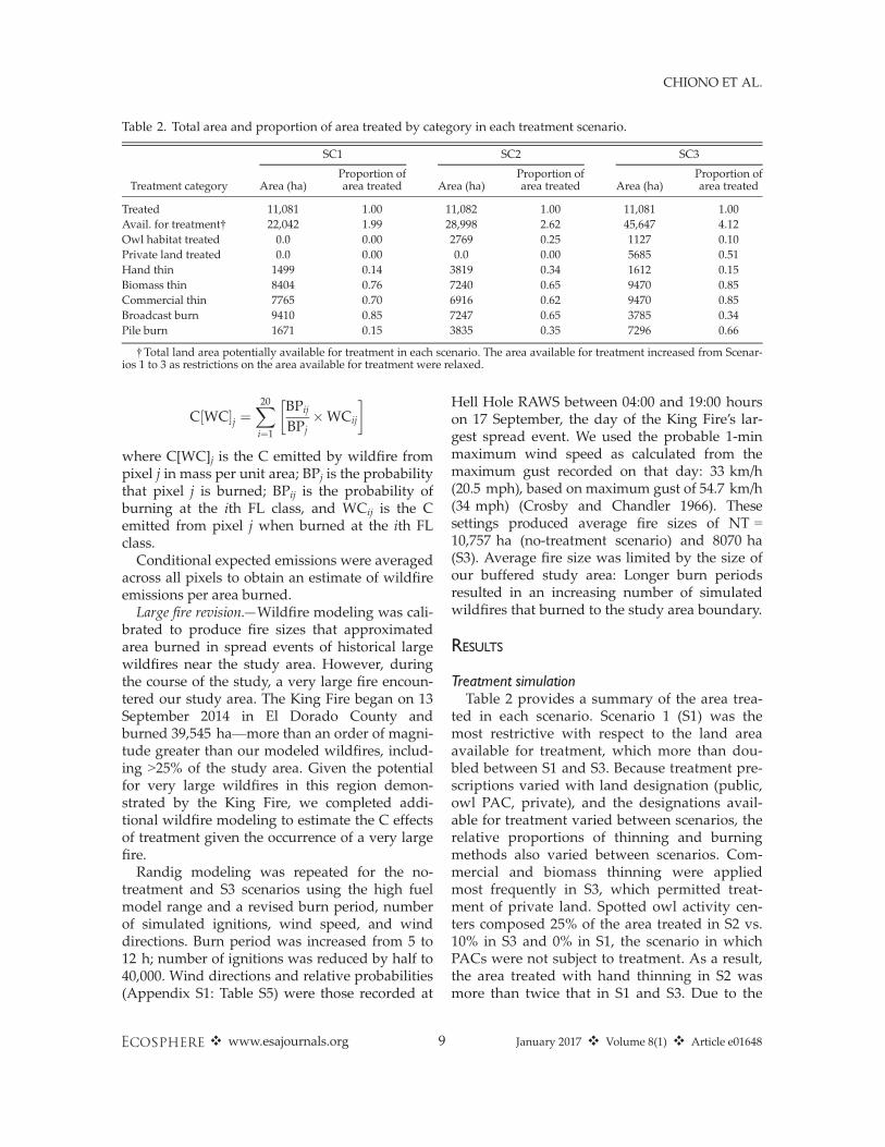
Treatment simulationTable 2 provides a summary of the area trea-

ted in each scenario. Scenario 1 (S1) was themost restrictive with respect to the land areaavailable for treatment, which more than dou-bled between S1 and S3. Because treatment pre-scriptions varied with land designation (public,owl PAC, private), and the designations avail-able for treatment varied between scenarios, therelative proportions of thinning and burningmethods also varied between scenarios. Com-mercial and biomass thinning were appliedmost frequently in S3, which permitted treat-ment of private land. Spotted owl activity cen-ters composed 25% of the area treated in S2 vs.10% in S3 and 0% in S1, the scenario in whichPACs were not subject to treatment. As a result,the area treated with hand thinning in S2 wasmore than twice that in S1 and S3. Due to the

Table 2. Total area and proportion of area treated by category in each treatment scenario.

Treatment category

SC1 SC2 SC3

Area (ha)Proportion ofarea treated Area (ha)

Proportion ofarea treated Area (ha)

Proportion ofarea treated

Treated 11,081 1.00 11,082 1.00 11,081 1.00Avail. for treatment† 22,042 1.99 28,998 2.62 45,647 4.12Owl habitat treated 0.0 0.00 2769 0.25 1127 0.10Private land treated 0.0 0.00 0.0 0.00 5685 0.51Hand thin 1499 0.14 3819 0.34 1612 0.15Biomass thin 8404 0.76 7240 0.65 9470 0.85Commercial thin 7765 0.70 6916 0.62 9470 0.85Broadcast burn 9410 0.85 7247 0.65 3785 0.34Pile burn 1671 0.15 3835 0.35 7296 0.66

†Total land area potentially available for treatment in each scenario. The area available for treatment increased from Scenar-ios 1 to 3 as restrictions on the area available for treatment were relaxed.


CHIONO ET AL.

inclusion of PACs in S2 and both PACs and pri-vate land in S3, the proportion of area treatedwith pile burning increased between S1 and S3,while broadcast burn area exhibited an oppositetrend. Despite the variation in land designationsavailable for treatment, the pattern of treat-ment placement was generally similar betweenscenarios, with treatments concentrated in thecentral and eastern portions of the study area(Figs. 4, 5).

Landscape-scale burn probability and fire hazardConditional burn probability.—The pixel-to-pixel

change in CBP between the untreated scenarioand each treatment scenario is mapped in Figs. 4(LO FM) and 5 (HI FM). Treatment reduced land-scape burn probability by approximately 50%(Table 3), from 0.0124 (NT) to 0.0062 (S1), 0.0059(S2), and 0.0055 (S3). Within treatment units, aver-age CBP fell by 69–76% to 0.0033–0.0035; outsideof treated stands, CBP fell to 0.0060–0.0069. Some

Fig. 4. Low fuel model range treatment locations and difference in conditional burn probability (CBP) and con-ditional flame length (CFL) (untreated-treated) for each treatment scenario. Negative values indicate an increasein CBP or CFL, while positive values represent a reduction. CBP is the likelihood that a pixel will burn given asingle ignition on the landscape and assuming the simulation conditions described in Appendix S1: Table S1 andin the text. Conditional flame length is the probability-weighted flame length, given these same assumptions.


CHIONO ET AL.

increases in CBP were also observed, particularlyfor the low fuel model range (Fig. 4).

The influence of treatment on owl PAC likeli-hood of burning was similar to that observedfor stands in general. For treated PACs, averageCBP fell by ~70% relative to no treatment for thesame stands. Although PACs were not eligiblefor treatment in S1, all treatment scenarios had alarge impact on estimated PAC CBP. AveragePAC CBP was reduced from 0.013 to 0.0063 inS1, 0.0049 in S2, and 0.0054 in S3, a 49–64%decrease relative to PACs in the no-treatmentlandscape (Table 3).

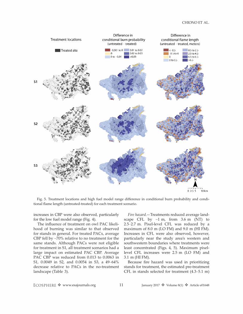
Fire hazard.—Treatments reduced average land-scape CFL by ~1 m, from 3.6 m (NT) to2.5–2.7 m. Pixel-level CFL was reduced by amaximum of 8.0 m (LO FM) and 9.0 m (HI FM).Increases in CFL were also observed, however,particularly near the study area’s western andsouthwestern boundaries where treatments wereleast concentrated (Figs. 4, 5). Maximum pixel-level CFL increases were 2.5 m (LO FM) and3.1 m (HI FM).Because fire hazard was used in prioritizing

stands for treatment, the estimated pre-treatmentCFL in stands selected for treatment (4.3–5.1 m)

Fig. 5. Treatment locations and high fuel model range difference in conditional burn probability and condi-tional flame length (untreated-treated) for each treatment scenario.


CHIONO ET AL.

was greater than in stands not selected (3.2–3.3 m). After treatment, average CFL within trea-ted stands fell to 1.3 (S1 and S2) and 1.7 m (S3).CFL in untreated stands was also reduced as aresult of the influence of treatments on firespread and intensity. CFL fell by 0.5–0.8 m (9–16%) relative to CFL in the same stands withinthe no-treatment landscape (Table 4).

Although spotted owl PACs were not treatedin S1, relative to PACs in the NT landscape,PAC CFL was reduced by 10% (to 3.2 m) in S1.Treating PACs had a much larger impact onpotential fire intensity, however. Average trea-ted PAC CFL fell to 1.3 and 1.4 m in S2 and S3,respectively.

Carbon consequences of landscape fueltreatments

Prior to treatment, aboveground landscapecarbon totaled 147.05 tonnes/ha, on average.Treatments removed 14% of pre-treatment Cfrom treated stands, or 23.74 tonnes/ha, totaling

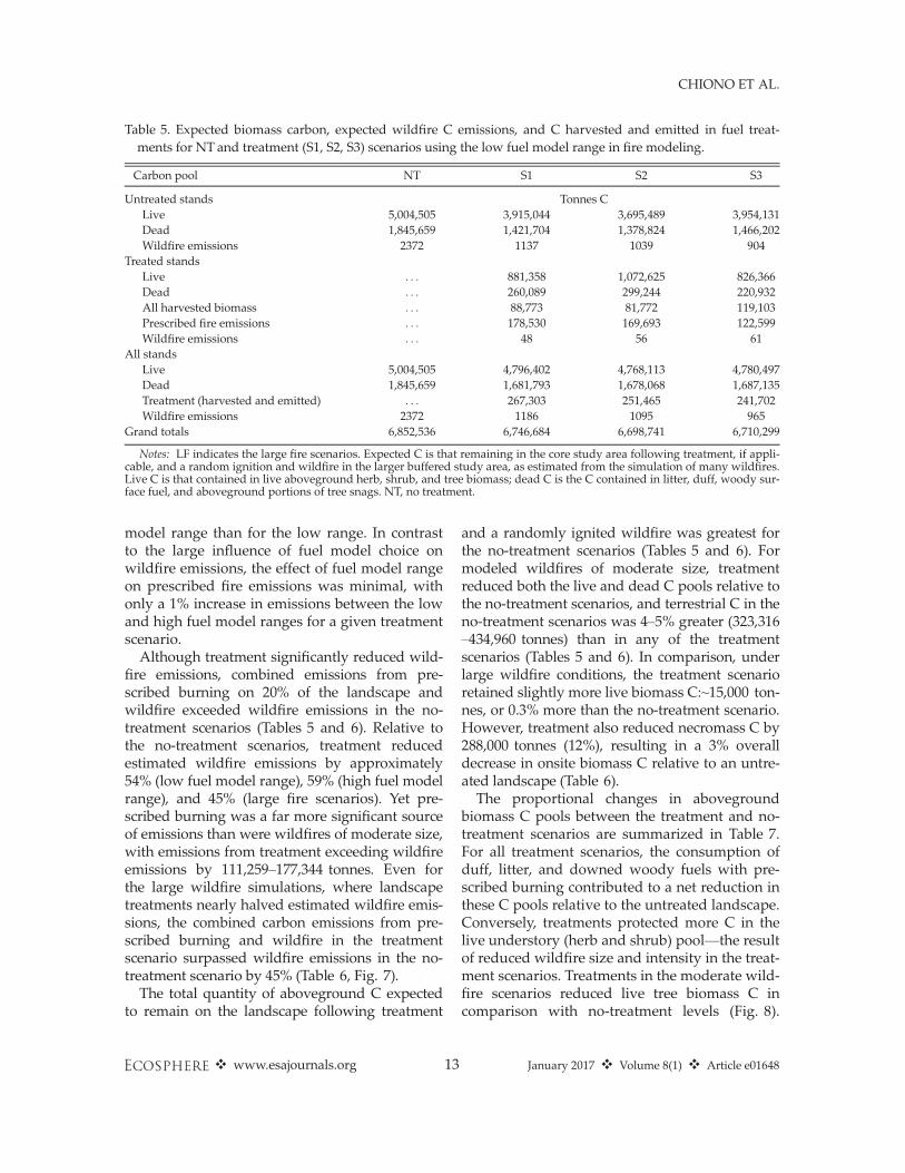
81,772–119,103 tonnes of C in harvested biomassand merchantable material (Tables 5 and 6).Both the treatment scenarios and the choice of

fuel models were important influences on esti-mated C emissions from burning. As the leastrestrictive treatment scenario in terms of treat-ment location and the only scenario to includetreatment of private land, where broadcast burn-ing was precluded as a treatment option, the S3treatment scenario was associated with the low-est wildfire and prescribed burning emissions(Tables 5 and 6). For each treatment scenario,expected wildfire emissions increased by morethan an order of magnitude between the low andhigh fuel model ranges. This difference was theresult of increasing fire intensity as well as wild-fire size. Average wildfire size nearly doubledbetween fuel model ranges in the treatment sce-narios and tripled in the no-treatment scenario(Fig. 6). For a given treatment scenario, wildfireemissions on a per hectare basis were approxi-mately two tonnes greater for the high fuel

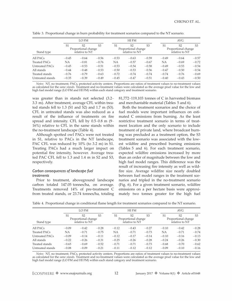
Table 3. Proportional change in burn probability for treatment scenarios compared to the NT scenario.

Stand type

LO FM HI FM AVG

S1 S2 S3 S1 S2 S3 S1 S2 S3Proportional change

relative to NTProportional change


relative to NT

All PACs �0.45 �0.64 �0.56 �0.53 �0.63 �0.59 �0.49 �0.64 �0.57Treated PACs NA �0.81 �0.76 NA �0.57 �0.67 NA �0.69 �0.72Untreated PACs �0.45 �0.53 �0.51 �0.53 �0.54 �0.58 �0.49 �0.53 �0.54All stands �0.44 �0.48 �0.53 �0.50 �0.53 �0.56 �0.47 �0.50 �0.54Treated stands �0.76 �0.79 �0.63 �0.72 �0.74 �0.74 �0.74 �0.76 �0.69Untreated stands �0.35 �0.39 �0.49 �0.45 �0.47 �0.51 �0.40 �0.43 �0.50

Notes: NT, no treatment; PACs, protected activity centers. Proportions are ratios of treatment values to no-treatment valuesas calculated for the same stands. Treatment and no-treatment values were calculated as the average pixel value for the low andhigh fuel model range (LO FM and HI FM) within each stand category and treatment scenario.

Table 4. Proportional change in conditional flame length for treatment scenarios compared to the NT scenario.

Stand type

LO FM HI FM AVG

S1 S2 S3 S1 S2 S3 S1 S2 S3Proportional change



relative to NT

All PACs �0.09 �0.42 �0.28 �0.12 �0.43 �0.27 �0.10 �0.42 �0.28Treated PACs NA �0.71 �0.75 NA �0.71 �0.73 NA �0.71 �0.74Untreated PACs �0.09 �0.14 �0.11 �0.12 �0.17 �0.14 �0.10 �0.16 �0.13All stands �0.22 �0.26 �0.31 �0.25 �0.26 �0.28 �0.24 �0.26 �0.30Treated stands �0.65 �0.69 �0.52 �0.71 �0.71 �0.73 �0.68 �0.70 �0.62Untreated stands �0.08 �0.09 �0.21 �0.11 �0.12 �0.12 �0.09 �0.10 �0.16

Notes: NT, no treatment; PACs, protected activity centers. Proportions are ratios of treatment values to no-treatment valuesas calculated for the same stands. Treatment and no-treatment values were calculated as the average pixel value for the low andhigh fuel model range (LO FM and HI FM) within each stand category and treatment scenario.


CHIONO ET AL.

model range than for the low range. In contrastto the large influence of fuel model choice onwildfire emissions, the effect of fuel model rangeon prescribed fire emissions was minimal, withonly a 1% increase in emissions between the lowand high fuel model ranges for a given treatmentscenario.

Although treatment significantly reduced wild-fire emissions, combined emissions from pre-scribed burning on 20% of the landscape andwildfire exceeded wildfire emissions in the no-treatment scenarios (Tables 5 and 6). Relative tothe no-treatment scenarios, treatment reducedestimated wildfire emissions by approximately54% (low fuel model range), 59% (high fuel modelrange), and 45% (large fire scenarios). Yet pre-scribed burning was a far more significant sourceof emissions than were wildfires of moderate size,with emissions from treatment exceeding wildfireemissions by 111,259–177,344 tonnes. Even forthe large wildfire simulations, where landscapetreatments nearly halved estimated wildfire emis-sions, the combined carbon emissions from pre-scribed burning and wildfire in the treatmentscenario surpassed wildfire emissions in the no-treatment scenario by 45% (Table 6, Fig. 7).

The total quantity of aboveground C expectedto remain on the landscape following treatment

and a randomly ignited wildfire was greatest forthe no-treatment scenarios (Tables 5 and 6). Formodeled wildfires of moderate size, treatmentreduced both the live and dead C pools relative tothe no-treatment scenarios, and terrestrial C in theno-treatment scenarios was 4–5% greater (323,316–434,960 tonnes) than in any of the treatmentscenarios (Tables 5 and 6). In comparison, underlarge wildfire conditions, the treatment scenarioretained slightly more live biomass C:~15,000 ton-nes, or 0.3% more than the no-treatment scenario.However, treatment also reduced necromass C by288,000 tonnes (12%), resulting in a 3% overalldecrease in onsite biomass C relative to an untre-ated landscape (Table 6).The proportional changes in aboveground

biomass C pools between the treatment and no-treatment scenarios are summarized in Table 7.For all treatment scenarios, the consumption ofduff, litter, and downed woody fuels with pre-scribed burning contributed to a net reduction inthese C pools relative to the untreated landscape.Conversely, treatments protected more C in thelive understory (herb and shrub) pool—the resultof reduced wildfire size and intensity in the treat-ment scenarios. Treatments in the moderate wild-fire scenarios reduced live tree biomass C incomparison with no-treatment levels (Fig. 8).

Table 5. Expected biomass carbon, expected wildfire C emissions, and C harvested and emitted in fuel treat-ments for NT and treatment (S1, S2, S3) scenarios using the low fuel model range in fire modeling.

Carbon pool NT S1 S2 S3

Untreated stands Tonnes CLive 5,004,505 3,915,044 3,695,489 3,954,131Dead 1,845,659 1,421,704 1,378,824 1,466,202Wildfire emissions 2372 1137 1039 904

Treated standsLive . . . 881,358 1,072,625 826,366Dead . . . 260,089 299,244 220,932All harvested biomass . . . 88,773 81,772 119,103Prescribed fire emissions . . . 178,530 169,693 122,599Wildfire emissions . . . 48 56 61

All standsLive 5,004,505 4,796,402 4,768,113 4,780,497Dead 1,845,659 1,681,793 1,678,068 1,687,135Treatment (harvested and emitted) . . . 267,303 251,465 241,702Wildfire emissions 2372 1186 1095 965

Grand totals 6,852,536 6,746,684 6,698,741 6,710,299

Notes: LF indicates the large fire scenarios. Expected C is that remaining in the core study area following treatment, if appli-cable, and a random ignition and wildfire in the larger buffered study area, as estimated from the simulation of many wildfires.Live C is that contained in live aboveground herb, shrub, and tree biomass; dead C is the C contained in litter, duff, woody sur-face fuel, and aboveground portions of tree snags. NT, no treatment.


CHIONO ET AL.

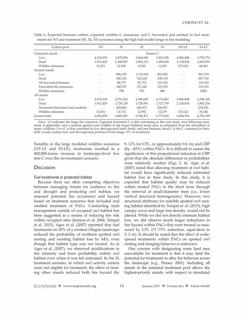
Notably, in the large modeled wildfire scenarios(NT-LF and S3-LF), treatments resulted in a400,000-tonne increase in landscape-level livetree C over the no-treatment scenario.

DISCUSSION

Fuel treatments in protected habitatBecause there are often competing objectives

between managing forests for resilience to fireand drought and protecting owl habitat, weassessed potential fire occurrence and hazardbased on treatment scenarios that included andomitted treatment of PACs. Conducting fuelsmanagement outside of occupied owl habitat hasbeen suggested as a means of reducing fire riskwithin occupied sites (Jenness et al. 2004, Tempelet al. 2015). Ager et al. (2007) reported that fueltreatments on 20% of a western Oregon landscapereduced the probability of northern spotted owlnesting and roosting habitat loss by 44%, eventhough that habitat type was not treated. As inAger et al. (2007), we observed modifications infire intensity and burn probability within owlhabitat even when it was left untreated. In the S1treatment scenario, in which owl activity centerswere not eligible for treatment, the effect of treat-ing other stands reduced both fire hazard (by

9–12% for CFL, or approximately 0.4 m) and CBP(by ~45%) within PACs. It is difficult to assess thesignificance of this proportional reduction in CBPgiven that the absolute differences in probabilitieswere relatively modest (Figs. 3, 4). Ager et al.(2007) noted that allowing treatment of owl habi-tat would have significantly reduced estimatedhabitat loss in their study. In this study, it isexpected that habitat quality may be reducedwithin treated PACs in the short term throughthe removal of small-diameter trees (i.e., lowervertical structural heterogeneity). However, twostructural attributes for suitable spotted owl nest-ing habitat identified by Tempel et al. (2015), highcanopy cover and large tree density, would not bealtered. While we did not directly estimate habitatloss, we did observe much larger reductions infire hazard within PACs that were treated as mea-sured by CFL (71–75% reduction, equivalent to2–3 m). It should be noted that the effect of wide-spread treatments within PACs on spotted owlnesting and foraging behavior is unknown.One concern with designating some land area

unavailable for treatment is that it may limit thepotential for treatments to alter fire behavior acrossthe landscape (e.g., Finney 2001). Including allstands in the potential treatment pool allows thehighest-priority stands, with respect to simulated

Table 6. Expected biomass carbon, expected wildfire C emissions, and C harvested and emitted in fuel treat-ments for NT and treatment (S1, S2, S3) scenarios using the high fuel model range in fire modeling.

Carbon pool NT S1 S2 S3 NT-LF S3-LF

Untreated stands Tonnes CLive 4,910,239 3,879,854 3,664,690 3,923,358 4,586,898 3,750,774Dead 1,912,429 1,448,947 1,403,313 1,489,629 2,130,034 1,605,591Wildfire emissions 31,831 12,934 12,001 11,293 137,622 68,061

Treated standsLive . . . 896,670 1,115,918 853,503 . . . 847,374Dead . . . 280,182 325,628 238,130 . . . 247,744All harvested biomass . . . 88,773 81,772 119,103 . . . 119,103Prescribed fire emissions . . . 180,357 171,247 123,539 . . . 123,539Wildfire emissions . . . 798 951 986 . . . 8285

All standsLive 4,910,239 4,776,524 4,780,607 4,776,861 4,586,898 4,598,148Dead 1,912,429 1,729,129 1,728,941 1,727,759 2,130,034 1,853,334Treatment (harvested and emitted) . . . 282,862 265,971 254,921 . . . 254,921Wildfire emissions 31,831 13,732 12,952 12,279 137,622 76,346

Grand totals 6,854,499 6,802,247 6,788,471 6,771,820 6,854,554 6,782,749

Notes: LF indicates the large fire scenarios. Expected terrestrial C is that remaining in the core study area following treat-ment, if applicable, and a random ignition and wildfire in the larger buffered study area, as estimated from the simulation ofmany wildfires. Live C is that contained in live aboveground herb, shrub, and tree biomass; dead C is the C contained in litter,duff, woody surface fuel, and aboveground portions of tree snags. NT, no treatment.


CHIONO ET AL.

fire spread, to be treated, which would be expectedto achieve the greatest modification of landscapefire behavior and effects. In the present study,although the land area potentially available fortreatment more than doubled between S1 and S3,landscape-level effects of treatment on modeledfire risk and hazard were fairly similar (comparedwith the no-treatment landscape, all-stand CBP fellby 47% and 54% in S1 and S3, while CFL fell by24% and 30%). Dow et al. (2016) also found thatincorporating modest restrictions on treatmentarea availability (24% of the landscape unavail-able) had minimal consequences for modeled firesize and hazard. The modest changes in estimatedfire metrics we observed may also be due to simi-larity in the general pattern of treatment placementbetween scenarios, which probably led to similar

effects on landscape-level fire behavior. The trueeffect of increasing the land area available for treat-ment may be partially obscured by the varyingfrequency of treatment prescriptions between sce-narios. For example, the hand thinning treatmentsapplied within PACs would be expected to have amilder effect on potential wildfire behavior thanmore severe prescriptions, and hand thinning wastwice as common in S2 as in the other scenarios.

Terrestrial carbon and burning emissionsLandscape treatments reduced wildfire emis-

sions by reducing the emissions produced per areaburned by wildfire as well as average wildfire size.On average, wildfires in the treated landscapesreleased 19.3–21.6 tonnes C/ha, while wildfires inthe untreated landscapes released 23.4–25.4 tonnesC/ha. Modeled wildfires decreased in size by 7%(low fuel model range), 36% (high fuel modelrange), and 25% (large fire scenario) relative tountreated landscapes (Fig. 6). Since the burn per-iod for simulated wildfires was held constantbetween scenarios, this reduction in average wild-fire size is the result of reduced spread ratesderived from fuel treatments.Despite the influence of treatments on wildfire

intensity, size, and expected emissions, treatment-related emissions exceeded the avoided wildfireemissions conferred by treatment. Prescribedburning in our study, a combination of broadcast

Fig. 6. Wildfire size relative frequency distributionsfrom wildfire simulations. Bar color represents no-treatment (NT) and treatment scenarios (S1–S3).

Fig. 7. Carbon emissions (tonnes) from wildfire andprescribed burning. X-axis labels indicate no-treatment(NT) and treatment scenarios (S1–S3); subscriptsdenote fuel model ranges used in fire modeling(L: low, H: high). Large fire scenarios, which weremodeled with the high fuel model range only, are indi-cated by LF.


CHIONO ET AL.

and pile burning, released 11.1–16.3 tonnes C/ha.For comparison, studies conducted in comparableforest types have estimated prescribed fire emis-sions of 12.7 tonnes C/ha (warm, dry ponderosapine habitat types; Reinhardt and Holsinger 2010)

and 14.8 tonnes C/ha (an old-growth mixed-conifer reserve in the southern Sierra Nevada;North et al. 2009a). Relative to the approximately158,000 tonnes C emitted in prescribed burning,avoided wildfire emissions, at 1186–19,551 tonnesfor wildfires of moderate size, were small. A simi-lar study in southern Oregon with average mod-eled wildfires of 2350 and 3500 ha (treatment andno-treatment scenarios, respectively) found thattreatments reduced expected wildfire emissionsby 6157 tonnes of C (Ager et al. 2010).Surface fuels, represented with surface fuel

models in commonly used modeling software,are the most influential inputs determining pre-dicted fire behavior (Hall and Burke 2006). Firebehavior, fire sizes, and emissions in this studyvaried according to fuel model assignment, high-lighting the importance of selecting the appropri-ate fuel model to represent fuel conditions (seeCollins et al. 2013). We show a 12- to 14-foldchange in wildfire emissions due solely to thechoice of fuel models (Tables 5 and 6). Indeed,the range of fuel models used in recent studiesinvestigating fuel treatments and simulated firebehavior in mixed-conifer forests is noteworthy.Incorporating a range of fuel models into analy-ses such that outcome variability can be reportedfacilitates comparison of effects across studies.Our estimates of the aboveground C benefits

of treatment under the moderate wildfire scenar-ios, with average fire sizes of ≤2133 ha, are likelyconservative. The effect of modeled wildfire sizeon the C consequences of fuel treatment was con-siderable, emphasizing the importance of thisvariable in studies of the climate benefits of treat-ment. Avoided wildfire emissions resulting fromtreatment increased to 61,276 tonnes C whenlarge wildfires (8070–10,757 ha) were simulated.The treatment scenario, given large wildfires,also protected a greater portion of live tree C. Ifthe ~40,000-ha King Fire is representative of themagnitude of future wildfires in the region, Caccounting should improve with respect to treat-ment favorability. Similarly, if multiple wildfireswere to encounter the study area within theeffective lifespan of treatments, the C gains asso-ciated with avoided emissions in the treatmentscenarios would increase.Our approach to estimating the C conse-

quences of fuel treatments has a number of limita-tions. A full accounting of treatment effects

Table 7. Proportional change in expected carbon bybiomass pool for treatment scenarios compared tothe no-treatment landscape.

Treatmentscenario

Standingdead

Down deadwood

Forestfloor

Herb/shrub

Livetree

S1 0.04 �0.17 �0.13 0.14 �0.04S2 0.01 �0.16 �0.12 0.14 �0.04S3 �0.01 �0.15 �0.10 0.16 �0.04S3-LF �0.16 �0.13 �0.08 0.17 0.00

Notes: For example, a value of �0.10 represents a 10% dec-line in biomass C from the no-treatment scenario. Treatmentand no-treatment values were calculated as the average of lowand high fuel model range values, except in the case of thelarge fire (LF) scenarios, which were modeled for the high fuelmodel range only. Expected C is that remaining after a randomignition and wildfire in the buffered study area as estimatedfrom simulating 80,000 ignitions (LF: 40,000 ignitions).

C pool categories are those reported in Forest VegetationSimulator Carbon Reports. Standing dead: aboveground por-tion of standing dead trees, Down dead wood: woody surfacefuels, Forest floor: litter and duff, Herb/shrub: herbs and shrubs,Live tree: aboveground portion of live trees.

Fig. 8. Expected carbon contained in abovegroundlive and dead tree biomass. Expected C is that remain-ing in the core study area following treatment (if appli-cable) and a single random ignition within the largerbuffered study area. X-axis labels indicate no-treatment (NT) and treatment scenarios (S1–S3); sub-scripts denote fuel model ranges used in fire modeling(L: low, H: high). Large fire scenarios, which weremodeled for the high fuel model range only, are indi-cated by LF.


CHIONO ET AL.

would project through time the consequences ofboth treatment andwildfire. Our analysis is static,incorporating only the short-term C costs andbenefits of treatment. Simulating wildfire in theyear immediately following treatment maximizesthe apparent benefits of treatment. Over time, assurface fuels accumulate and vegetation regener-ates, maintenance would be required to retain theeffectiveness of treatments (Martinson and Omi2013), increasing the C costs of reduced firehazard. In addition, the C contained in fire-killedbiomass will ultimately be emitted to the atmo-sphere, although biomass decay could be delayedthrough conversion to long-lived wood productssuch as building materials (Malmsheimer et al.2011). It is also important to note that our analysisdid not include stochastic wildfire occurrence.Estimates of burn probability in the present studyare not estimates of the likelihood of wildfireoccurrence based on historical fire sizes and fre-quency (e.g., Preisler et al. 2004, Mercer andPrestemon 2005, Brillinger et al. 2006), but ratherare conditional on a single randomly ignitedwildfire within the buffered study area.

CONCLUSIONS

Our findings generally support those of Camp-bell et al. (2011), who concluded from an analysisof fire-prone western forests that the C costs oftreatments are likely to outweigh their benefitsunder current depressed fire frequencies. In amore recent paper, Campbell and Ager (2013) con-cluded that “none of the fuel treatment simulationscenarios resulted in increased system carbon,”primarily from the low incidences of treated areasbeing burned by wildfire. However, our interpre-tation of these findings differs from those dis-cussed in Campbell et al. (2011) and Campbelland Ager (2013), especially in light of recent andprojected future trends in fire activity (Westerlinget al. 2011, Miller and Safford 2012, Dennisonet al. 2014). The current divergence of increasingsurface air temperatures and low fire activity isunlikely to be sustained, further suggestinggreater future fire activity (Marlon et al. 2012). Ifincreased fire activity is realized, then the likeli-hood of a given area being burned in a wildfireincreases. This differs from the simple increase instand-level fire frequency modeled by Campbellet al. (2011) because increases in fire likelihood are

not necessarily associated with correspondingdecreases in fire severity, as assumed by Campbellet al. (2011). Increased fire likelihood could verywell lead to positive feedbacks in fire severity, andultimately to vegetation type conversion (Coppo-letta et al. 2016)—effects that would have signifi-cant implications for carbon storage.Due to the significant emissions associated

with treatment and the low likelihood that wild-fire will encounter a given treatment area, forestmanagement that is narrowly focused on Caccounting alone would favor the no-treatmentscenarios. Landscape treatments protected more Cin live tree biomass only when large wildfireswere simulated. While treatment favorabilityimproved with large wildfire simulation, the no-treatment scenario still produced fewer emissionsthan the treatment scenario. Given the potentialfor large wildfire in the region as demonstratedby the 2014 King Fire, and the increasing fre-quency of large wildfires and area burned in Cali-fornia expected from climate modeling studies(Lenihan et al. 2008, Westerling et al. 2011), wesuggest that future studies of fuel treatment–wild-fire–C relationships should incorporate the poten-tial for large wildfires at a frequency greater thanthose observed over the last 20–30 yr. Others haveargued that treatments to increase forest resilienceshould be a stand-alone, top land managementpriority independent of other ecosystem valuessuch as carbon sequestration and fire hazardreduction (Stephens et al. 2016a).We also note that the potential benefits of fuels

management are not restricted to avoided wild-fire emissions. Here, we show that landscape fueltreatments can alter fire hazard across the land-scape both within and outside of treated stands,and have the potential to affect the likelihood ofburning and fire intensity within protected Cali-fornia spotted owl habitat. Underscoring the riskto sensitive habitat, the 2014 King Fire encoun-tered 31 PACs within our study area, leading tothe greatest single-year decline in habitat occu-pancy recorded over a 23-yr study period (Joneset al. 2016). Modest simulated treatments withinactivity centers significantly reduced potentialfire intensity relative to both the no-treatmentlandscape and a treatment scenario that did notpermit treatment within PACs, indicating thatactive management may be desirable to protecthabitat in the long term (Roloff et al. 2012).


CHIONO ET AL.

However, treatments conducted outside of owlhabitat also reduced wildfire hazard.

ACKNOWLEDGMENTS

We are grateful to a number of individuals for shar-ing their time and fuel treatment and fire modelingexpertise: Nicole Vaillant (ArcFuels), Alan Ager andAndrew McMahan (carbon estimation), and CoeliHoover (harvest simulations in FVS-FFE). Brian Ebertand Dana Walsh of the Eldorado National Forest pro-vided invaluable advice on weather inputs for firemodeling and on designing fuel treatment prescrip-tions. Ken Somers, Operations Forester on the BlodgettForest Research Station, gave advice concerning tim-ber management on private land. We also thank twoanonymous reviewers, whose comments greatlyimproved this article. The California Energy Commis-sion provided funding for this project.

LITERATURE CITED

Ager, A. A., B. Bahro, and K. Barber. 2006. Automatingthe fireshed assessment process with ArcGIS.Pages 163–167 in P. L. Andrews and B. W. Butler(Comps), Fuels Management–How to MeasureSuccess: Conference Proceedings, Portland, OR,March 28–30, 2006. Proceedings RMRS-P-41.USDA Forest Service, Rocky Mountain ResearchStation, Fort Collins, Colorado, USA.

Ager, A. A., M. A. Finney, B. K. Kerns, and H. Maffei.2007. Modeling wildfire risk to northern spotted owl(Strix occidentalis caurina) habitat in Central Oregon,USA. Forest Ecology and Management 246:45–56.

Ager, A. A., M. A. Finney, A. McMahan, and J. Cathcart.2010. Measuring the effect of fuel treatments on for-est carbon using landscape risk analysis. NaturalHazards and Earth System Science 10:2515–2526.

Ager, A. A., N. M. Vaillant, D. E. Owens, S. Brittain,and J. Hamann. 2012. Overview and exampleapplication of the Landscape Treatment Designer.Pages 11. General Technical Report PNW-GTR-859.USDA Forest Service, Pacific Northwest ResearchStation, Portland, Oregon, USA.

Barbour, M. G., and R. A. Minnich. 2000. Californianupland forests and woodlands. Pages 131–164 inM. Barbour and W. Billings, editors. North Ameri-can terrestrial vegetation. Cambridge UniversityPress, Cambridge, UK.

Bias, M. A., and R. Guti�errez. 1992. Habitat associationsof California spotted owls in the central SierraNevada. Journal of Wildlife Management 56:584–595.

Bond, M. L., R. Gutierrez, A. B. Franklin, W. S.LaHaye, C. A. May, and M. E. Seamans. 2002.

Short-term effects of wildfires on spotted owl sur-vival, site fidelity, mate fidelity, and reproductivesuccess. Wildlife Society Bulletin 30:1022–1028.

Brillinger, D., H. Preisler, and J. Benoit. 2006. Proba-bilistic risk assessment for wildfires. Environ-metrics 17:623–633.

Campbell, J. L., and A. A. Ager. 2013. Forest wildfire,fuel reduction treatments, and landscape carbonstocks: a sensitivity analysis. Journal of Environ-mental Management 121:124–132.

Campbell, J. L., M. E. Harmon, and S. R. Mitchell.2011. Can fuel-reduction treatments really increaseforest carbon storage in the western US by reduc-ing future fire emissions? Frontiers in Ecology andthe Environment 10:83–90.

Cathcart, J., A. A. Ager, A. McMahan, M. Finney, andB. Watt. 2010. Carbon benefits from fuel treat-ments. Pages 61–80 in T. B. Jain, R. T. Graham, andJ. Sandquist, editors. Integrated management ofcarbon sequestration and biomass utilizationopportunities in a changing climate: Proceedings ofthe 2009 National Silviculture Workshop, Boise,Idaho, June 15–18, 2009. USDA Forest Service Pro-ceedings RMRS-P-61, Rocky Mountain ResearchStation, Fort Collins, Colorado, USA.

Chatfield, A. H. 2005. Habitat selection by a Californiaspotted owl population: a landscape scale analysisusing resource selection functions. Thesis. Univer-sity of Minnesota,, St. Paul, Minnesota, USA.

Collins, B. M., H. A. Kramer, K. Menning, C. Dilling-ham, D. Saah, P. A. Stine, and S. L. Stephens. 2013.Modeling hazardous fire potential within a com-pleted fuel treatment network in the northernSierra Nevada. Forest Ecology and Management310:156–166.

Collins, B. M., S. L. Stephens, J. J. Moghaddas, andJ. Battles. 2010. Challenges and approaches in plan-ning fuel treatments across fire-excluded forestedlandscapes. Journal of Forestry 108:24–31.

Collins, B. M., S. L. Stephens, G. B. Roller, and J. J.Battles. 2011. Simulating fire and forest dynamicsfor a landscape fuel treatment project in the SierraNevada. Forest Science 57:77–88.

Coppoletta, M., K. E. Merriam, and B. M. Collins.2016. Post-fire vegetation and fuel developmentinfluences fire severity patterns in reburns. Ecologi-cal Applications 26:686–699.

Crookston, N. L., and A. O. Finley. 2008. yaimpute: anr package for knn imputation. Journal of StatisticalSoftware 23:1–16.

Crookston, N. L., M. Moeur, and D. L. Renner. 2002.User’s guide to the most similar neighbor imputa-tion program version 2. General Technical ReportRMRS-GTR-96. USDA Forest Service, RockyMountain Research Station, Ogden, Utah, USA.


CHIONO ET AL.

Crosby, J., and C. Chandler. 1966. Get the most fromyour windspeed observations. Fire Control Notes27:12–13.

Dailey, S., J. Fites, A. Reiner, and S. Mori. 2008. Firebehavior and effects in fuel treatments and pro-tected habitat on the Moonlight fire. Fire BehaviorAssessment Team. www.fs.fed.us/adaptivemanagement/projects/FBAT/docs/MoonlightFinal_8_6_08.pdf

Dennison, P. E., S. C. Brewer, J. D. Arnold, and M. A.Moritz. 2014. Large wildfire trends in the westernUnited States, 1984–2011. Geophysical ResearchLetters 41:2928–2933.

Dixon, G. E. 2002. Essential FVS: a user’s guide to theforest vegetation simulator. Pages 193. USDAForest Service, Forest Management Service Center,Fort Collins, Colorado, USA.

Dore, S., T. E. Kolb, M. Montes-Helu, B. W. Sullivan,W. D. Winslow, S. C. Hart, J. P. Kaye, G. W. Koch,and B. A. Hungate. 2008. Long-term impact of astand-replacing fire on ecosystem CO2 exchange ofa ponderosa pine forest. Global Change Biology14:1–20.

Dore, S., M. Montes-Helu, S. C. Hart, B. A. Hungate,G. W. Koch, J. B. Moon, A. J. Finkral, and T. E. Kolb.2012. Recovery of ponderosa pine ecosystem carbonand water fluxes from thinning and stand-replacingfire. Global Change Biology 18:3171–3185.

Dow, C. J., B. M. Collins, and S. L. Stephens. 2016.Incorporating resource protection constraints in ananalysis of landscape fuel-treatment effectivenessin the Northern Sierra Nevada, California, USA.Environmental Management 57:1–15.

Eidenshink, J., B. Schwind, K. Brewer, Z. Zhu,B. Quayle, and S. Howard. 2007. A project for mon-itoring trends in burn severity. Fire Ecology 3:3–21.

Evans, A. M., and A. J. Finkral. 2009. From renewableenergy to fire risk reduction: a synthesis of biomassharvesting and utilization case studies in US for-ests. GCB Bioenergy 1:211–219.

Finkral, A. J., and A. M. Evans. 2008. The effects of athinning treatment on carbon stocks in a northernArizona ponderosa pine forest. Forest Ecology andManagement 255:2743–2750.

Finney, M. A. 2001. Design of regular landscape fueltreatment patterns for modifying fire growth andbehavior. Forest Science 47:219–228.

Finney, M. A. 2002. Fire growth using minimum traveltime methods. Canadian Journal of Forest Research32:1420–1424.

Finney, M. A. 2006. An overview of FlamMap firemodeling capabilities. Pages 213–220 in P. L.Andrews and B. W. Butler, editors. Proceedings ofFuels Management–How to Measure Success.Research Paper RMRS-P-41. USDA Forest Service,

Rocky Mountain Research Station, Portland,Oregon, USA.

Finney, M. A., R. C. Seli, C. W. McHugh, A. A. Ager,B. Bahro, and J. K. Agee. 2007. Simulation of long-term landscape-level fuel treatment effects on largewildfires. International Journal of Wildland Fire16:712–727.

Ful�e, P. Z., J. E. Crouse, J. P. Roccaforte, and E. L. Kalies.2012. Do thinning and/or burning treatments inwestern USA ponderosa or Jeffrey pine-dominatedforests help restore natural fire behavior? ForestEcology and Management 269:68–81.

Gaines, W. L., R. J. Harrod, J. Dickinson, A. L. Lyons,and K. Halupka. 2010. Integration of Northernspotted owl habitat and fuels treatments in theeastern Cascades, Washington, USA. Forest Ecol-ogy and Management 260:2045–2052.

Gaines, W. L., R. A. Strand, and S. D. Piper. 1997.Effects of the hatchery complex fires on northernspotted owls in the eastern Washington Cascades.Pages 123–129 in J. N. Greenlee, editor. Proceedingsof the Fire Effects on Rare and Endangered Speciesand Habitats Conference, Coeur D’Alene, Idaho.International Association of Wildfire and Forestry,Hot Springs, South Dakota, USA.

Hall, S. A., and I. C. Burke. 2006. Considerations forcharacterizing fuels as inputs for fire behaviormodels. Forest Ecology and Management 227:102–114.

Hoover, C., and S. Rebain. 2008. The Kane Experimen-tal Forest carbon inventory: carbon reporting withFVS. Pages 13–15 in R. N. Havis and N. L.Crookston, editors. Third Forest Vegetation Simu-lator Conference, Fort Collins, Colorado, February13–15, 2007. USDA Forest Service, Rocky MountainResearch Station, Fort Collins, Colorado, USA.

Hurteau, M., and M. North. 2009. Fuel treatmenteffects on tree-based forest carbon storage andemissions under modeled wildfire scenarios. Fron-tiers in Ecology and the Environment 7:409–414.

Hurteau, M. D., and M. North. 2010. Carbon recoveryrates following different wildfire risk mitigationtreatments. Forest Ecology and Management 260:930–937.

Hurteau, M. D., M. T. Stoddard, and P. Z. Ful�e. 2011.The carbon costs of mitigating high-severity wild-fire in southwestern ponderosa pine. GlobalChange Biology 17:1516–1521.

Jenness, J. S., P. Beier, and J. L. Ganey. 2004. Associa-tions between forest fire and Mexican spotted owls.Forest Science 50:765–772.

Jones, G. M., R. Guti�errez, D. J. Tempel, S. A. Whitmore,W. J. Berigan, and M. Z. Peery. 2016. Megafires: anemerging threat to old-forest species. Frontiers inEcology and the Environment 14:300–306.


CHIONO ET AL.

http://www.fs.fed.us/adaptivemanagement/projects/FBAT/docs/MoonlightFinal_8_6_08.pdf



Laymon, S. A. 1988. Ecology of the spotted owl in thecentral Sierra Nevada, California. Dissertation.University of California, Berkeley, California, USA.

Lenihan, J. M., D. Bachelet, R. P. Neilson, andR. Drapek. 2008. Response of vegetation distribution,ecosystem productivity, and fire to climate changescenarios for California. Climatic Change 87:215–230.

Lydersen, J. M., B. M. Collins, E. E. Knapp, G. B. Roller,and S. Stephens. 2015. Relating fuel loads to over-storey structure and composition in a fire-excludedSierra Nevada mixed conifer forest. InternationalJournal of Wildland Fire 24:484–494.

Malmsheimer, R., J. Bowyer, J. Fried, E. Gee, R. Islar,R. Miner, I. E. Munn, E. Oneil, and W. C. Stewart.2011. Managing forests because carbon matters:integrating energy, products, and land manage-ment policy. Journal of Forestry 109:S7–S50.

Marlon, J. R., et al. 2012. Long-term perspective onwildfires in the western USA. Proceedings of theNational Academy of Sciences of the United Statesof America 109:E535–E543.

Martinson, E. J., and P. N. Omi. 2002. Performance offuel treatments subjected to wildfires. Pages 7–13in P. N. Omi and L. A. Joyce, editors. Conferenceon Fire, Fuel Treatments, and Ecological Restora-tion. USDA Forest Service, Rocky MountainResearch Station, Fort Collins, Colorado, USA.

Martinson, E. J., and P. N. Omi. 2013. Fuel treatmentsand fire severity: a meta-analysis. Pages 38. USDAForest Service, Rocky Mountain Research Station,Fort Collins, Colorado, USA.

Mayer, K. E., and W. F. Laudenslayer. 1988. A guide towildlife habitats of California. California Depart-ment of Forestry and Fire Protection, Sacramento,California, USA.

McKenzie, D., Z. Gedalof, D. L. Peterson, and P. Mote.2004. Climatic change, wildfire, and conservation.Conservation Biology 18:890–902.

Mercer, D. E., and J. P. Prestemon. 2005. Comparingproduction function models for wildfire risk analy-sis in the wildland–urban interface. Forest Policyand Economics 7:782–795.

Miller, J. D., and H. Safford. 2012. Trends in wildfireseverity: 1984 to 2010 in the Sierra Nevada, ModocPlateau, and southern Cascades, California, USA.Fire Ecology 8:41–57.

Miller, J., H. Safford, M. Crimmins, and A. Thode.2009. Quantitative evidence for increasing forestfire severity in the Sierra Nevada and southernCascade mountains, California and Nevada, USA.Ecosystems 12:16–32.

North, M. 2012. Managing Sierra Nevada forests. PSW-GTR-237. USDA Forest Service, Pacific SouthwestResearch Station, Albany, California, USA.

North, M. P., and M. D. Hurteau. 2011. High-severitywildfire effects on carbon stocks and emissions infuels treated and untreated forest. Forest Ecologyand Management 261:1115–1120.

North, M., M. Hurteau, and J. Innes. 2009a. Fire sup-pression and fuels treatment effects on mixed-conifer carbon stocks and emissions. EcologicalApplications 19:1385–1396.

North, M., P. A. Stine, K. O’Hara, W. Zielinski, andS. Stephens. 2009b. An ecosystem managementstrategy for Sierran mixed-conifer forests. GeneralTechnical Report PSW-GTR-220. USDA ForestService, Pacific Southwest Research Station,Albany, California, USA.

Parisien, M.-A., S. Snetsinger, J. A. Greenberg, C. R.Nelson, T. Schoennagel, S. Z. Dobrowski, andM. A. Moritz. 2012. Spatial variability in wildfireprobability across the western United States. Inter-national Journal of Wildland Fire 21:313–327.

Penman, J., M. Gytarsky, T. Hiraishi, T. Krug, D. Kruger,R. Pipatti, L. Buendia, K. Miwa, T. Ngara, andK. Tanabe. 2003. Good practice guidance for landuse, land-use change and forestry. Institute forGlobal Environmental Strategies for the Intergov-ernmental Panel on Climate Change, Hayama,Kanagawa, Japan.

Pollet, J., and P. N. Omi. 2002. Effect of thinning andprescribed burning on crown fire severity inponderosa pine forests. International Journal ofWildland Fire 11:1–10.

Prather, J. W., R. F. Noss, and T. D. Sisk. 2008. Realversus perceived conflicts between restoration ofponderosa pine forests and conservation of theMexican spotted owl. Forest Policy and Economics10:140–150.

Preisler, H. K., D. R. Brillinger, R. E. Burgan, andJ. Benoit. 2004. Probability based models forestimation of wildfire risk. International Journal ofWildland Fire 13:133–142.

Rebain, S., E. Reinhardt, N. Crookston, S. Beukema,W. Kurz, and J. Greenough. 2009. The fire and fuelsextension to the Forest Vegetation Simulator.Addendum to RMRS-GTR-119. USDA ForestService and ESSA Technologies Ltd, Fort Collins,Colorado, USA.

Reinhardt, E. D., and N. L. Crookston. 2003. The fireand fuels extension to the forest vegetation simula-tor. Pages 209. RMRS-GTR-116. USDA Forest Ser-vice, Rocky Mountain Research Station, Ogden,Utah, USA.

Reinhardt, E., and L. Holsinger. 2010. Effects offuel treatments on carbon-disturbance relation-ships in forests of the northern Rocky Mountains.Forest Ecology and Management 259:1427–1435.


CHIONO ET AL.

Reinhardt, E. D., R. E. Keane, D. E. Calkin, and J. D.Cohen. 2008. Objectives and considerations forwildland fuel treatment in forested ecosystems ofthe interior western United States. Forest Ecologyand Management 256:1997–2006.

Ritchie, M. W., C. N. Skinner, and T. A. Hamilton.2007. Probability of tree survival after wildfire inan interior pine forest of northern California:effects of thinning and prescribed fire. Forest Ecol-ogy and Management 247:200–208.

Roloff, G. J., S. P. Mealey, and J. D. Bailey. 2012. Com-parative hazard assessment for protected species ina fire-prone landscape. Forest Ecology and Man-agement 277:1–10.

Rothermel, R. C. 1972. A mathematical model for pre-dicting fire spread in wildland fuels. ResearchPaper INT-115. USDA Forest Service, Intermoun-tain Forest and Range Experiment Station, Ogden,Utah, USA.

Safford, H. D. 2008. Fire severity in fuel treatments:American River Complex fire, Tahoe National Forest,California. Unpublished Report. USDA Forest ServicePacific Southwest Region, Vallejo, California, USA.

Schmidt, D. A., A. H. Taylor, and C. N. Skinner. 2008.The influence of fuels treatment and landscapearrangement on simulated fire behavior, SouthernCascade range, California. Forest Ecology andManagement 255:3170–3184.

Scott, J. H., and R. E. Burgan. 2005. Standard firebehavior fuel models: a comprehensive set for usewith Rothermel’s surface fire spread model.General Technical Report RMRS-GTR-153. USDAForest Service Rocky Mountain Research Station,Fort Collins, Colorado, USA.

Scott, J. H., M. P. Thompson, and J. W. Gilbertson-Day.2016. Examining alternative fuel managementstrategies and the relative contribution of NationalForest System land to wildfire risk to adjacenthomes–a pilot assessment on the Sierra NationalForest, California, USA. Forest Ecology and Man-agement 362:29–37.

Smith, J. E., and L. S. Heath. 2002. A model of forestfloor carbon mass for United States forest types.Research Paper NE-722. USDA Forest Service,Northeastern Research Station, Newtown Square,Pennsylvania, USA.

Stephens, S. L. 2005. Forest fire causes and extent onUnited States Forest Service lands. InternationalJournal of Wildland Fire 14:213–222.

Stephens, S. L., B. M. Collins, E. Biber, and P. Z. Ful�e.2016a. US federal fire and forest policy: emphasiz-ing resilience in dry forests. Ecosphere 7:e01584.

Stephens, S. L., J. D. Miller, B. M. Collins, M. P. North,J. J. Keane, and S. L. Roberts. 2016b. Wildfireimpacts on California Spotted Owl nesting habitatin the Sierra Nevada. Ecosphere 7:e01584.

Stephens, S. L., J. J. Moghaddas, B. R. Hartsough, E. E.Y. Moghaddas, and N. E. Clinton. 2009. Fuel treat-ment effects on stand-level carbon pools, treat-ment-related emissions, and fire risk in a SierraNevada mixed-conifer forest. Canadian Journal ofForest Research 39:1538–1547.

Stephens, S. L., et al. 2012. Fuel treatment impacts onestimated wildfire carbon loss from forests in Mon-tana, Oregon, California, and Arizona. Ecosphere3:1–17.

Tempel, D., et al. 2015. Evaluating short- and long-term impacts of fuels treatments and simulatedwildfire on an old-forest species. Ecosphere 6:1–19.

USDA Forest Service. 2004. Sierra Nevada Forest PlanAmendment. Final supplemental environmentalimpact statement. Record of decision. PublicationR5-MB-046. USDA Forest Service, Pacific South-west Region, Vallejo, California, USA.

Van Wagner, C. E. 1977. Conditions for the start andspread of crown fire. Canadian Journal of ForestResearch 7:23–34.

Verner, J., K. S. McKelvey, B. R. Noon, R. Guti�errez,G. I. Gould Jr., and T. W. Beck. 1992. Assessment ofthe current status of the California spotted owl,with recommendations for management. Pages3–27 in J. Verner, K. S. McKelvey, B. R. Noon,R. Guti�errez, G. I. Gould Jr., and T. W. Beck, edi-tors. The California Spotted Owl: a technicalassessment of its current status. PSW-GTR-133.USDA Forest Service, Albany, California, USA.

Westerling, A., B. Bryant, H. Preisler, T. Holmes,H. Hidalgo, T. Das, and S. Shrestha. 2011. Climatechange and growth scenarios for California wild-fire. Climatic Change 109:445–463.

Westerling, A. L., H. G. Hidalgo, D. R. Cayan, andT. W. Swetnam. 2006. Warming and earlier Springincrease Western U.S. Forest Wildfire Activity.Science 313:940–943.

Wiedinmyer, C., and M. D. Hurteau. 2010. Prescribedfire as a means of reducing forest carbon emissionsin the Western United States. EnvironmentalScience & Technology 44:1926–1932.

SUPPORTING INFORMATION

Additional Supporting Information may be found online at: http://onlinelibrary.wiley.com/doi/10.1002/ecs2.1648/full


CHIONO ET AL.

http://onlinelibrary.wiley.com/doi/10.1002/ecs2.1648/full

http://onlinelibrary.wiley.com/doi/10.1002/ecs2.1648/full

Landscape‐scale fuel treatment and wildfire … · Landscape-scale fuel treatment and...

Documents

Transcript of Landscape‐scale fuel treatment and wildfire … · Landscape-scale fuel treatment and...