Landscape similarity, retrieval, and machine mapping of physiographic units

Jaroslaw Jasiewiczb,a, Pawel Netzelc,a, Tomasz F. Stepinskia

aSpace Informatics Lab, Dept. of Geography, University of Cincinnati, Cincinnati, OH 45221-0131, USAbGeoecology and Geoinformation Institute, Adam Mickiewicz University, Dziegielowa 27, 60-680 Poznan, PolandcDept. of Climatology and Atmospheric Protection, University of Wroclaw, Kosiby 6/8, 51-621, Wroclaw, Poland

Abstract

We introduce landscape similarity - a numerical measure that assesses affinity between two landscapes on the basisof similarity between the patterns of their constituent landform elements. Such a similarity function provides coretechnology for a landscape search engine - an algorithm that parses the topography of a study area and finds all placeswith landscapes broadly similar to a landscape template. A landscape search can yield answers to a query in realtime, enabling a highly effective means to explore large topographic datasets. In turn, a landscape search facilitatesauto-mapping of physiographic units within a study area. The country of Poland serves as a test bed for these novelconcepts. The topography of Poland is given by a 30 m resolution DEM. The geomorphons method is applied to thisDEM to classify the topography into ten common types of landform elements. A local landscape is represented bya square tile cut out of a map of landform elements. A histogram of cell-pair features is used to succinctly encodethe composition and texture of a pattern within a local landscape. The affinity between two local landscapes isassessed using the Wave-Hedges similarity function applied to the two corresponding histograms. For a landscapesearch the study area is organized into a lattice of local landscapes. During the search the algorithm calculatesthe similarity between each local landscape and a given query. Our landscape search for Poland is implementedas a GeoWeb application called TerraEx-Pl and is available at http://sil.uc.edu/. Given a sample, or a number ofsamples, from a target physiographic unit the landscape search delineates this unit using the principles of supervisedmachine learning. Repeating this procedure for all units yields a complete physiographic map. The application of thismethodology to topographic data of Poland results in the delineation of nine physiographic units. The resultant mapbears a close resemblance to a conventional physiographic map of Poland; differences can be attributed to geologicaland paleogeographical input used in drawing the conventional map but not utilized by the mapping algorithm.

Keywords: Landscape similarity, Landscape search, Physiographic mapping, Pattern recognition, Supervisedclassification, Web application

1. Introduction

Regionalization and mapping are the core elementsof geomorphologic analysis. Traditionally, these tasksare carried out by analysts who rely on their visual per-ception of data and expert knowledge to delineate unitsof land surface within a given study area. Possible tar-get units of mapping include – in order of increasingcomplexity – landform elements, landforms and land-scapes (see Minar and Evans (2008) for a descriptionof the hierarchical partitioning of land surfaces). Withthe increasing availability of medium-to-high resolutionDEMs covering the entire land surface of the Earth aswell as surfaces of other planets and because of theslowness, expense, and subjectivity of manual analysis,there is a significant interest in automating the process

of geomorphologic mapping.

In this paper we present a novel methodology for theautomated delineation of landscape types within a studyarea. To the best of our knowledge no previous work hasaddressed this issue directly by taking into account thecomplexity of landscape units as described, for exam-ple, by Minar and Evans (2008). Instead, previous workconcentrated on the automatic classification of land-forms – surface units of lesser complexity then land-scapes. In practice, however, the methods employedin previous works tended to generalize the notion of“landform” to the point where the resultant maps (Iwa-hashi and Pike, 2007; Dragut and Eisank, 2012) delin-eate units that could be best described as physiographicunits. Therefore, we will be able to compare the results

Preprint submitted to Geomorphology July 22, 2014

of our mapping methodology with the results of previ-ous auto-mapping techniques.

All previous methods share a common framework.They are classification schemes that assign a label toan areal unit on the basis of geomorphometric vari-ables (Evans, 1972; Pike, 1988; MacMillan et al., 2004;Olaya, 2009) and/or their statistics calculated fromDEM values at a given unit and/or from its immedi-ate neighborhood. The first such classification schemewas devised by Hammond (1954) and was later imple-mented as a computer algorithm (Dikau et al., 1991;Gallant et al., 2005). Other landform classificationschemes were proposed by Meybeck et al. (2001) andIwahashi and Pike (2007) using different combinationsof geomorphometric variables. Recently, Dragut andEisank (2012) introduced the concept of Object-BasedImage Analysis (OBIA) to classification of landforms.In their method a DEM is first segmented into multi-cellunits which are homogeneous with respect to geomor-phometric variables, and those units, rather then DEMcells, are the objects of classification.

The approach presented in this paper is based on dif-ferent principles. We start with the concept of similar-ity between landscapes. Using this concept we designa computational framework for a landscape search andfor auto-mapping of landscape types or physiographicunits. According to the taxonomy of Minar and Evans(2008) landscapes are patterns of landforms which inturn are composites of landform elements. We skip themiddle level of this hierarchy and consider landscape tobe a pattern of landform elements over a site of inter-est. A similarity between two landscapes is defined asa single number that encapsulates all aspects of compo-sitional and configurational alikeness between two pat-terns of landform elements.

Despite the great variability of local landscapeswithin a study area (a landscape at any specific siteis unique in its details), there are a limited number ofsemantically different landscape types that can be dis-cerned. We consider landscape types to be tantamountto physiographic units – regions of the study area hav-ing internal uniformity of landscape and clearly differ-ent from surrounding regions. A measure of similaritybetween landscapes enables the algorithmic identifica-tion of landscape types. The landscape search engine isan algorithm which, given a sample landscape (a query),parses the entire study area and retrieves sites havinglandscapes similar to that of the query. The set of all re-trieved landscapes constitutes the landscape type exem-plified by the query. An auto-mapper of physiographicunits is an algorithm which delineates a study area intoan exclusive and exhaustive set of physiographic re-

gions.Note that an auto-mapping algorithm that utilizes

our framework could be based on the machine learningprinciples of either unsupervised learning (Duda et al.,2001) or supervised learning (Mehryar et al., 2012).An unsupervised learning algorithm delineates physio-graphic units without any guidance from an analyst byclustering similar landscapes. The number and charac-ter of these units emerge from the data and need to be in-terpreted afterward. An unsupervised learning mappingapproach is most useful for the exploration of a studyarea with little prior knowledge about its physiography,like, for example, a planetary surface (Bue and Stepin-ski, 2006). A supervised learning algorithm delineatesstudy area into an a priori known set of units on thebasis of landscape samples provided by an analyst. Asupervised approach is most useful when there is someprior knowledge about the physiography of a study areabut objective delineation of units is desired. Note thatthe previous auto-mapping methods mentioned aboveare often referred to as “unsupervised” because they re-quire no interaction between an algorithm and an ana-lyst. However, they are not based on either supervisedor unsupervised machine learning principles. They clas-sify cells/segments into a priori defined landform types(a supervised aspect) but numerical criteria for belong-ing to a given type depends on the statistics of the data(an unsupervised aspect).

In this paper we focus on a supervised variant of ourauto-mapping algorithm with the delineation of phys-iographic units achieved by repeated application of thelandscape search algorithm. The methodology pre-sented here is general and applies to any study area forwhich a DEM of sufficient quality is available. We illus-trate the steps in our method using an entire territory ofthe country of Poland (represented by a 30 m resolutionDEM) as a study area.

2. Analytical and computational framework

Because our methodology consists of several compo-nents, we start by describing its overall framework – alogical structure of several separate concepts and theircomputational implementations that together underpinour approach to landscape retrieval and mapping.

A schema of our analytical framework is shown inFig. 1. The topography of a study area (Fig. 1A) is usedas input data. Because we are concerned with the searchfor and mapping of spatially extensive areal units (of thesize of physiographic units), a study area would typi-cally cover a region which is very large in comparisonto the resolution of a DEM. In this paper we consider

2

(B) Map of landforms(A) DEMLattice of local landscapes(C)

(F) Landscape search

(G) Physiographic map

(D) Landscape representation or signature

(E) Landscape similarity measure

ridge

shoulder

spurpit

slopehollow

footslope

valley!at

peak

Figure 1: Schema showing an analytic framework of our methodology.

a study area containing the entire country of Polandat 30 m resolution (see Section 3 for details). Thefirst element of our method is an automatic mappingof landform elements from a DEM (A→B transition onFig. 1). This step could be achieved using several differ-ent methods (Wood, 1996; Dikau et al., 1995; Jasiewiczand Stepinski, 2013a) developed to classify DEM cellsinto a small number of categorical labels indicating anelementary form of a local surface. Extending our pre-vious work we use the geomorphons method (Jasiewiczand Stepinski, 2013a) that allows for a direct, single-step classification of landform elements. The geomor-phons method provides a fast and robust tool for achiev-ing the A→B transition. It classifies DEM cells intothe ten most common landform elements: flat, peak,pit, ridge, valley, shoulder, footslope, spur, and hollow(Fig. 1B). We have computed 30 m resolution maps oflandform elements using the geomorphons method forPoland and, additionally for the United States. Thesemaps can be explored and compared to a hillshade ren-dition of topography using our GeoWeb tools availableat http://sil.uc.edu/.

The second element of our method is the conver-sion of a map of landform elements into a lattice oflocal landscapes (B→C transition on Fig. 1). We op-erationally define a local landscape as a square-shapedtile cut out of the map of landform elements. The sizeof a tile should be large enough so that local landscapescontain non-trivial mosaics of landform elements, butsmall enough to ensure a diversity of landscape types in

the study area. The tiles are arranged in a lattice of locallandscapes and together they cover the entire study area(Fig. 1C).

An overall, quantitative measure of similarity be-tween two landscapes is the key concept of our method-ology. To the best of our knowledge this concept hasnot been discussed with respect to its application to ge-omorphology. However, it has been studied in the con-text of landscape ecology (Wickham and Norton, 1994;Allen and Walsh, 1996; Cain et al., 1997) where the no-tion of landscape pertains to patterns of land use/landcover (LULC) categories rather than to the patterns oflandform elements. There are two components of land-scape similarity: (1) a concise numerical representa-tion of landscape pattern hereafter referred to as a land-scape signature (Fig. 1D) and (2) a similarity function(Fig. 1E) that uses this representation to calculate anumber that encapsulates the overall degree of “alike-ness” or affinity between two landscapes. In landscapeecology, a signature is a vector of landscape indices(O’Neill et al., 1988; Herzog and Lausch, 2001) andthe Euclidean distance is used as the similarity function.Our choices for the landscape signature and similarityfunction are different from those used in the LULC con-text because the pattern characteristics of landform el-ements are different from those of LULC patterns (seedetails in Section 4).

The landscape search (Fig. 1F) utilizes a query-andretrieval technique to find all local landscapes similarto a sample landscape (also referred to as a “query”).

3

A query doesn’t have to be one of the local landscapespredefined by a lattice of tiles, and it doesn’t have tobe taken from the study area, however, in this paper allqueries are samples from the study area. The search isperformed by calculating the similarity between a queryand each of the local landscapes. The result of thissearch is a “similarity map” (Fig. 1F) with locationscolored in accordance with their similarity to a query.A landscape type exemplified by a query can be delin-eated as a set of all locations having a similarity to thequery which is larger than a specified threshold.

Using several different templates and a repeated ap-plication of the landscape search we partition the studyarea into a set of physiographic units (Fig. 1G) corre-sponding to landscape types exemplified by respectivetemplates. Using each template as a query we obtain aset of similarity maps, which, when reconciled, yield asingle map of physiographic units (for details see Sec-tion 6).

3. Study area

Our study area is the country of Poland. Poland isa country in Central Europe located between latitudes49◦ and 55◦ N and longitudes 14◦ and 25◦ E. Its surfacearea is 312,685 km2. The territory of Poland exhibitsa number of different landscape types including coastalplains in the northernmost part of the country, young–undenudated and old–denuded post-glacial lowlands ofdifferent ages in the northern and central parts, and up-lands and mountains in the southern part. A color ren-dition of Poland’s topography is shown in Fig. 2A.

A traditional physiographic map of Poland (hereafterreferred to as a “reference” map) has been obtained bygeneralizing a physigraphic regionalisation of Polandproposed by Kondracki (2002). The original Kondrackimap has been created manually on the basis of geomor-phological as well as geological and paleogeographicalinformation and includes many units, some of them de-lineated on the basis of regional position. The refer-ence map shown in Fig. 1B delineates only 12 phys-iographic units as described by its legend (Fig. 1C).They include surfaces formed during the last glaciac-tion (young morainic hills, young moraininc plateausand plains) and surfaces resulting from previous glacia-tion morphogenesis strongly modified by denudationalprocess during the last glaciation (old morainic plateausand hills, old morainic plains and old moraninc plainson older substratum). These units are frequently bun-dled together as “lowlands” on less specific maps orby global automatic classifiers based on geomorphome-tric variables like those by Iwahashi and Pike (2007) or

Dragut and Eisank (2012). On the other hand, our land-scape similarity-based methodology would be able tomap these units quite well using only topographic dataand without the benefit of additional information fromgeology and paleogeography.

The topographic data for Poland is a 1” integer-valued DEM (obtained from the Silesia University)which we reprojected to the PUWG92 coordinate sys-tem and converted by adaptive smoothing to a floating-point terrain model with a resolution of 30 m/cell. Ourfinal DEM is 21,696 × 24,692 cells. The 30 m/cell cat-egorical map of landform elements is calculated fromthis DEM using the geomorphons method (Jasiewiczand Stepinski, 2013a). This map was calculated usingthe following values for the two parameters requiredby the geomophons method: Search radius L =40cells (1200 m), and Flatness threshold t =0.8 degree.The geomorphons code is available for download fromhttp://sil.uc.edu/. The hillshade and the shaded relief ofthe DEM, as well as the map of landforms elements,are available for exploration using the GeoWeb toolTerraEx-Pl available from the same website.

4. Landscapes similarity

Being able to quantify the overall similarity betweentwo landscapes using a single number is a key elementof our methodology. In both landscape ecology and ge-omorphology landscapes can be considered as categor-ical spatial patterns, suggesting that we can apply simi-larity measures developed (Cain et al., 1997; Long et al.,2010; Kupfer et al., 2012) for LULC landscapes to pat-terns of landscape elements. However, this is not thecase as these two types of patterns have different char-acteristics. While the most important discriminant be-tween two LULC patterns is the presence or absenceof specific LULC categories, most terrain patterns con-tain all categories of landscape elements. This followsfrom the fact that terrain consists of a series of land-form elements, for example: valley, slope, ridge, slope,valley, etc. Thus, while LULC landscapes are predom-inantly distinguished from each other on the basis ofland cover composition, terrain landscapes are predom-inantly distinguished from each other on the basis oftheir texture or the spatial configuration of their basicelements. In addition, the nature of land surfaces dic-tates that landscape patterns are dominated by just twoelementary forms: “flats” in the lowlands and “slopes”in areas of higher relief. All other elementary forms,such as peaks, pits, ridges, valleys, footslopes, hollows,spurs, and shoulders are less abundant, but they are nev-ertheless crucial for characterizing terrain texture. In

4

Broad river valleys and pradolinas

Young morainic plateaus and plains- poorly or no denudated

Young morainic hills- poorly or no denudated

Old morainic plateaus and hillson older basement - denudated

Old morainic plateaus and hills - denudated

Old morainic planes - denudated

Medium mountains

Low mountains

Local depresions

Highlands and low mountains

Flat boggy plains

Coastal plains

A B C

25001200

700500300200150100

500

meters

1000 200 300 400 km

N

Figure 2: Topography and physiography of Poland. (A) Topographic map of Poland. (B) Reference physiographic map of Polandbased on the Kondracki (2002) concept. (C) Legend for the reference physiographic map.

designing a quantitative measure of similarity betweenlandscapes the contribution of these landform elementsmust be enhanced relative to their abundance.

In designing a landscape numerical signature we fol-low principles established in the field of Content-BasedImage Retrieval (CBIR) (Gevers and Smeulders, 2004;Datta et al., 2008; Lew et al., 2006) – another domainwhere the issue of similarity between two rasters, in thiscase images, has been studied. In CBIR a pattern sig-nature is calculated as a histogram of a pattern’s ”prim-itive features.” A histogram is a good choice for patternsignature because of its rotational invariance; two pat-terns rotated with respect to each other will have iden-tical histograms. Primitive features are simple mea-sures designed to provide small, local pieces of infor-mation about a pattern. For example, a landform ele-ment at a given cell could be a primitive feature, and ahistogram of all landform elements over the landscapecould be a landscape signature. Such signature would,however, reflect only the abundance of landform ele-ments in the landscape and would not characterize thelandscape well enough (see discussion above) for effec-tive comparison with other landscapes.

We use pairs of neighboring cells as primitive fea-tures as shown in Fig. 3A. This figure shows a small(8×8 cell) map of landform elements. Each cell inthis map generates eight pairs which are shown by ar-rows in the case of three cells selected as examples(an 8-connected neighborhood is assumed). For exam-ple, the leftmost of the three example cells shown onFig. 3A is labeled as “slope” and generates eight pairs:three slope-slope pairs, four slope-footslope pairs andone slope-channel pair. If a map of landform elementsmaps C different elements, there are (C2 + C)/2 dif-ferent possible types of neighboring cells. Because thegeomorphons-generated map has 10 different elements,

there are 55 different possible pairs of elements, exam-ples include: flat-flat, flat-slope, slope-peak, etc.

The design of the landscape signature (first describedby Barnsley and Barr (1996) in the context of landuse reclassification) simultaneously encodes the com-position and texture of the landscape in a simple his-togram. (Note that this histogram contains the same in-formation as a co-occurrence matrix (Haralick, 1986)).Fig. 3B illustrates how two different landscapes (de-picted by their maps of landform elements) are repre-sented by histograms of cell-pair features. The legendfor Fig. 3A also applies to the maps shown in Fig. 3B.Histograms of the cell-pair features have 55 bins, witheach bin height proportional to a number of cell-pairsbelonging to a cell-pair category as indicated by colorlabels shown between the two histograms. The highestbins usually correspond to pairs of same category cell-pairs; they encode the composition of the landscape.For example, histogram of landscape 1 is dominatedby flat-flat, slope-slope, and valley-valley bins, whereasthe histogram of landscape 2 is dominated by slope-slope, valley-valley, and ridge-ridge bins. The bins cor-responding to pairs of different cell categories encodethe texture of the landscape.

The similarity between two landscapes is calculatedusing their signatures (histograms of features) and asimilarity (or a distance) function. Note that a “dis-tance” is a measure of dissimilarity between two land-scapes and is thus the reverse of similarity. Choosingmost appropriate similarity/distance function is largelyan empirical decision. Cha (2007) provides a com-prehensive review of possible functions to calculatethe distance between two histograms. After extensiveexperimentation with different similarity measures wehave observed that a modified Wave-Hedges similarityfunction (Cha, 2007) measures similarity between land-

5

lan

dsc

ap

e 1

lan

dsc

ap

e 2

pattern features - pairs

of landform elements

Primitive features are

pairs of neighboring

landform elements

Histogram of pairs of neighboringlandform elements in landscape 1

Histogram of pairs of neighboringlandform elements in landscape 2

A B

peak

footslope

ridge

shoulder

spur

slope

hollow

valley

pit

!at

Figure 3: Landscape numerical signature. (A) Graph explaining pairs of neighboring landform elements as pattern primitive features.(B) Example of two landscapes and their corresponding signatures - histograms of primitive features.

scapes in a way that is most consistent with human per-ception. Let A and B denote two landscapes and Ah andBh denote their corresponding signatures (histograms).The similarity between these two landscapes is given bythe following formula:

sim(A, B) = sim(Ah, Bh) =1M

M∑i=1

min(Ahi , B

hi )

max(Ahi , B

hi )

(1)

where M is the number of positions in both histogramswhere at least one bin is non-zero and Ah

i and Bhi are

the values of bins in the i-th position. This measuretakes into account only the cell-pair features that arepresent in at least one of the two landscapes. It com-pares each pair of corresponding bins separately by di-viding a smaller bin value by its bigger counterpart. Theresult is a number between 0 and 1. Where the value ofone of the bins is 0, there is no similarity with respect tothis cell-pair feature between the two landscapes. If thevalues of both bins are identical, there is perfect similar-ity with respect to that cell-pair feature between the twolandscapes. The overall similarity is an arithmetic aver-age of all contributing similarities, its range is between0 (no similarity between landscapes) and 1 (landscapesare identical).

Note that in Eqn. (1) the contributions of all cell-pairfeatures to an overall similarity value are taken with thesame weight regardless of each feature’s abundance inthe landscape. This ensures that composition-relatedfeatures (pairs of same category cells) and texture-related features (pairs of different category cells) havethe same chance to contribute to the overall similarityvalue despite the dominance of composition-related fea-tures in all realistic histograms (see Fig. 3B). It alsoensures that landscape similarity will not be heavilyskewed by the relative abundance of the most commonlandscape elements – flat and slope. Other potential

similarity functions, like the Euclidean distance or theJensen-Shannon distance, are dominated by similarityof the most abundant features. As a result, when thosemeasures are applied to, for example, two landscapesboth dominated by the flat element but with differentsecondary elements, they would yield a high value ofsimilarity by focusing on the fact that both landscapesare basically flat. Frequently, this result will not corre-spond to the perception of an analyst for whom differentdepartures from flat terrain are associated with signifi-cant dissimilarity between the two landscapes. How-ever, the application of the similarity function given inEqn. (1) to this example would result in lower value ofsimilarity, more in agreement with how a human ana-lyst would determine the similarity between those twolandscapes.

5. Landscape search

The purpose of a landscape search engine is to en-able the discovery of locations containing landscapessimilar to a specified landscape of interest. Like othermore familiar search engines it works on the principleof query-and-retrieval. However, the spatial aspect oftopographic data calls for the presentation of search re-sults in a manner that is different from those employedin non-spatial search engines. For example, an Internetsearch engine returns only several results (web pages,images) which represent the “best-fit” results to a givenquery. In contrast, the output of a landscape search en-gine is a similarity map which visually shows a degreeof similarity to a query at all locations throughout theentire study area, thus providing geospatial context.

Fig. 4 illustrates the principle of the landscape search.Fig. 4A shows the topographic map of Poland with agreen-to-brown color gradient illustrating low-to-high

6

1.0

0.9

0.8

0.7

0.6

0.5

0.4

0.3

0.2

0.1

0.0

A

B1

B2

C

Figure 4: Concept of landscape search. (A) Topographic map of Poland. (B1) Shaded relief of query landscape. (B2) Map oflandform elements of query landscape (see Fig. 5 for legend). (C) Similarity map. See main text for additional informations.

elevations. The small black square in the lower-rightportion of the map indicates the location of a query.Fig. 4C shows the color-coded similarity values be-tween that query and all local landscapes covering theentire territory of Poland. Locations on the similaritymap which are shown in red are similar to the query;they are located along the southern border of Polandwithin a physiographic unit of medium mountains (seeFig. 2). Map locations shown in green are completelydissimilar to the query and correspond to lowlands. Maplocations shown in various shades of yellow are also dis-similar to the query, but less so than the locations shownin green; they correspond to highlands and low moun-tains in the south and young morainic hills in the north.

Implementation of the landscape search in softwarefollows our earlier design (Jasiewicz and Stepinski,2013b; Stepinski et al., 2014) meant for searching theNational Land Cover Database (NLCD) for U.S. loca-tions having similar patterns of LULC. We use an over-lapping sliding window approach. A square grid witha resolution of k raster cells is superimposed over theentire spatial extent of the study area. This grid forms abasis for the similarity map resulting from the query.Thus, the resultant similarity map has a resolution ktimes coarser than the map of landform elements. Wewill refer to cells of similarity map as “super-cells.” Thequery is executed by means of exhaustive evaluation -the value of landscape similarity is calculated betweenthe query tile (see section 2 to recall a definition of thetile) and all the local tiles assigned to the similarity grid.

The size of a tile is N×k. If N = 1 the tiles are identi-cal to super-cells and they don’t overlap with neighbor-ing tiles. However, in general, it is preferable to con-sider overlapping tiles (N > 1) to better accommodatethe continuous character of landscape. In this paper we

use k = 50 and N = 10 resulting in tile size of 15 km× 15 km and a similarity map with a resolution of 1.5km. Fig. 5 illustrates the relationship between tiles andsuper-cells. Fig. 5A shows the 30 m resolution map oflandform elements. The purple square denoted Q indi-cates a 15 km × 15 km tile containing the landscape tobe used as a query. Fig. 5B shows the 1.5 km resolu-tion similarity map. The clearly visible pixelation in-dicates super-cells; the color of each super-cell reflectsthe value of similarity between the query and the land-scape contained in the 15 km × 15 km tile centered onthis super-cell. The three examples of super-cell loca-tions are labeled L1, L2, and L3 respectively. Thesesuper-cells are outlined by a thin dashed line and theircorresponding tiles are outlined by a thick solid line.For example, a similarity value stored in the super-cellL1 indicates the similarity between the landscapes con-tained in tiles Q and L1.

In order to maximize the utility of the landscapesearch we have implemented it as a modern Internet ap-plication (called TerraEx-Pl) running in a web browser.TerraEx-Pl, available at http://sil.uc.edu/, is a comput-erized map application with all functionalities availablethrough an active web page (as Google Maps). It en-ables real-time landscape searches to be performed overthe country of Poland. The resultant similarity maps canbe downloaded as GeoTiff files for offline analysis.

6. Delineation of physiographic units

We now demonstrate how to divide the territory ofPoland into an exclusive and exhaustive set of phys-iographic units using a supervised learning approachthat utilizes the landscape search method described inthe previous section. Table 1 gives a description of

7

1.0

0.9

0.8

0.7

0.6

0.5

0.4

0.3

0.2

0.1

0.0peak

footslope

ridge

shoulder

spur

slope

hollow

valley

pit

at

A B

Q

L1

L2

L3Q

L3

L2

L1

Figure 5: Relationship between tiles and super-cells. (A) Map of landform elements. (B) Similarity map to query Q. Purple squarelabeled Q indicates location and spatial extent of a query landscape. Black squares labeled L1, l2, and L3 indicate locations andspatial extents of sample local landscapes. See main text for more details.

nine physiographic units we have selected for mapping.They correspond to the 12 regions presented on our ref-erence physiographic map (Fig. 2B). For auto-mappingwe did not select regions from Fig. 2B which refer totheir genesis rather than physiography as our methodworks (by our choice and design) only on the basis oflandscape morphology alone. Thus, “broad river valleysand pradolinas”, “costal plains”, and “flat boggy plains”are combined into “flat plains”, and “old morainic plainsand hills” and “old morainic plains and hills on olderbasement” are combined into a single unit. Also “localdepressions” are not selected as a unit to be mapped, buta new unit “inland dunes” is added.

Following the methodology of supervised learningwe selected a number of template landscapes for eachunit based on our expert knowledge. The third col-umn in Table 1 shows a number of landscapes usedas templates for a given unit. Altogether, 64 templatelandscapes where selected to represent the characteris-tic landscapes of various units. Locations of templatelandscapes and their samples are shown in Fig. 6.

We execute the landscape search with each templateserving in turn as a query. The result is 64 similaritymaps, each showing the spatial distribution of similar-ity to the given querying. It could be expected thatsimilarity maps stemming from the set of queries rep-resenting a single unit should be very similar to eachother. This is certainly the case for some sets of queries.For example, similarity maps for all 11 templates rep-resenting medium mountains (MM) are much the same.This means that landscape samples selected for mediummountains have all very similar terrain texture and thatthe entire unit of medium mountains has relatively uni-

form texture. On the other hand, similarity maps for12 templates representing young morainic plateaus andplains (YMPP) show marked differences. This is be-cause the set of YMPP landscape samples displays somevariance in terrain texture. This follows from the factthe terrain texture across the YMPP unit is relativelyless uniform than, for example, the terrain texture acrossthe MM unit. The fact that some units display an inter-nal variance of patterns is the reason for using a set ofdifferent landscape samples instead of a single sampleto represent a “typical” landscape.

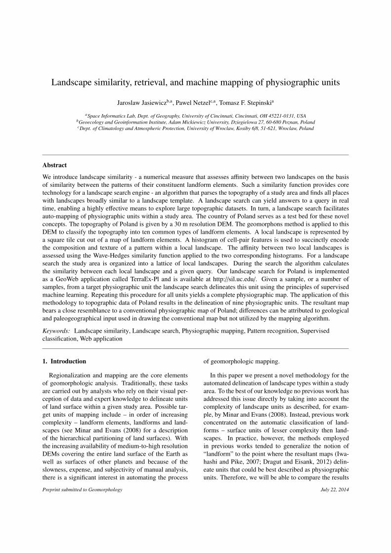
We average all similarity maps stemming from tem-plates representing a single unit. Because the values onany similarity map range from 0 to 1, the average mapsalso have the same range of values and can be inter-preted as a map showing the likelihood of local land-scapes belonging to a given unit. The average sim-ilarity (likelihood) maps for all nine units are shownin Fig. 7A. The most distinct physiographic units arethose for which likelihood maps are dominated by high(red) and low (green) values, thus clearly delineating aunit from the rest of the study area. Medium moun-tains (MM), low mountains (LM) and young morainichills (YMH) are such units. A unit for which the like-lihood map shows a lot of medium values marked byorange and yellow colors is less crisply defined. Ouralgorithm indicates that extended portions of the studyarea could be assigned to such unit but only with like-lihood that is relatively small. Highlands (HL), youngmorainic plateaus and plains (YMPP), dunes (DN), oldmorainic plateaus and hills(OMPH), and old morainicplains (OMP) are examples of such units. The likeli-hood map for flat plains (FP) unit does not show high

8

Table 1: Definitions of physiographic units

Name Abbreviation # of samples DescriptionMedium mountains MM 11 Areas above 1000 m asl, medium dense texture and high, sharp

relief, regular dendritic pattern, no flat areas.Low mountains LM 5 Areas between 500 and 1000 m asl, dense texture, medium and

sharp relief, regular dendritic pattern, no flat areas, limited amountof slopes.

Highlands HL 9 Areas between 300 and 500 m asl, dense texture, medium and highrelief, regular dendritic pattern, limited flat areas.

Young morainic hills YMH 10 Areas between 100 and 300 m asl, medium density texture, highrelief and irregular pattern, limited flat areas.

Young morainic plateausand plains

YMPP 12 Areas below 100-150 m asl, low and medium density texture, ir-regular pattern, significant amount of flat areas.

Inland dunes DN 3 Elevation mostly below 100 m asl, very high density of texture,characteristic pattern, no flat areas in dune fields.

Old morainic plateaus andhills

OMPH 4 Areas between 100 and 300 m asl, low density texture, low andsmooth relief, regular dendritic pattern, significant amount of flatareas.

Old morainic plains OMP 5 Areas between 100 and 300 m asl, low density texture, very smoothor flat relief, large amount of flat areas.

Flat plains FLP 7 Flat areas with very small addition of other forms.

MM

LM

HL

YMH

YMPP

DN

OMPH

OMP

FLP

MM LM HL

YMH YMPP DN

OMPH OMP FLP

A B

1000 200 300 400 km

Figure 6: A set of template landscapes. (A) Landform elements map of Poland with locations of template landscapes indicated bysquares having colors corresponding to units they exemplify (see legend to the right). (B) Nine sample landscapes (shown as mapsof landform elements), each representing one of nine units.

values at all. This does not mean that local sites havingflat landscapes are not similar to each other, but rather itreflects the nature of our similarity function (Eqn. (1))that shows relatively smaller values of similarity be-tween landscapes dominated by a single landform el-ements (flat) as it concentrates on differences betweentrace elements.

In the final step all nine likelihood maps are com-bined. This means that every super-cell temporarilystores nine values of likelihood, one for each unit. Thesevalues indicate the likelihood that a given super-cell be-longs to each of the possible units. In order to producea physiographic map of Poland we disambiguate thesenine possibilities by assigning to a super-cell a unit la-bel corresponding to the largest likelihood. This map is

shown in Fig. 7B; it represents the final product of ourcalculations.

This generated map can be compared to the refer-ence map (Fig. 2B) although we stress that referencemap does not represent “ground truth” in the machinelearning sense. Instead both maps are different mod-els of reality made using different methodologies anddifferent means. The reference map, like most man-ually created maps, delineates regions by delineatingtheir boundaries. The homogeneity of landscape pat-terns within a boundary is implicit. Our algorithm de-lineates units by establishing regions with homogeneouslandscape patterns. The boundaries between units areimplicit. Nevertheless, the two maps tell the same story.The landscape types in Poland are arranged in a pat-

9

1.0 0.9 0.8 0.7 0.6 0.5 0.4 0.3 0.2 0.1 0.0

MM LM HL YMH

YMPP DN OMPH OMP

FLP

MM

LM HL YMHYMPP

DN

OMPH

OMPFLP

BA

Figure 7: Delineation of physiographic units. (A) Spacial distributions of probability of belonging to a physiographic unit asindicated by a label. (B) The final, algorithm-delineated map of nine physiographic units across Poland.

tern of latitudinal belts (Lencewicz, 1937; Galon, 1972;Kondracki, 2002). These belts are the result of the gen-eral relief of Poland, with mountains and highlands inthe south and lowlands in the middle and the north.Because the overall pattern of uplifted areas dependsmostly on orography and its geological structure, thegeomorphometry of lowlands are the result of the di-minishing southward extent of successive Pleistoceneglaciations (Marks, 2005). Every glacial epoch left sev-eral to hundred meters of new deposits, which after re-treating revealed new, immature surfaces which becametargets of denudation processes (Dylik, 1952, 1956).The overall differences between the two maps are minorand can be attributed to geological and paleogeograph-ical inputs that went into the construction of referencemap but were intentionally omitted from our algorithmwhose goal was landscape comparison on the basis ofterrain patterns alone. For example, the region locatedjust south of the Notec pradolina in western Poland isclassified exclusively as the YMPP unit on the refer-ence map (Fig. 2B) up to the maximum extent of lastglaciation (Marks, 2005). The same region is dividedinto several units (YMPP, YMH, DN, OMPH) on ourmap (Fig. 7B) because of differences in topography. Lo-cally, the boundaries between corresponding units fromthe two maps are somewhat shifted, but the relative mer-its of specific delineations need to be discussed on a site-by-site case.

7. Discussion and Conclusions

In this paper we presented a new methodology en-abling the quantitative comparison of landscapes, asearch for landscapes similar to a given template, and,finally, the auto mapping of landscape types (or phys-iographic units). This methodology extends the field ofgeomorphometry - the science of quantitative land sur-face analysis - into the realm of content-based retrieval.Such an extension is significant because it opens up sev-eral new, practical possibilities.

First, our methodology provides for knowledge dis-covery through geomorphometry, as it makes possi-ble a convenient exploration of very large topographicdatasets (DEMs) in real time. Note that this is com-pletely different from the capacity to search a DEMand its derivatives by attribute value using SQL queriesbuilt into most GIS systems. Whereas SQL queriesretrieve individual DEM cells fulfilling predefined nu-merical conditions, our system retrieves entire land-scapes on the basis of their similarity to a template.The only analog to our methodology is Content-BasedImage Retrieval (CBIR) (Gevers and Smeulders, 2004;Datta et al., 2008; Lew et al., 2006) - the process of re-trieving desired images from a large collection on thebasis of features such as color, texture and shape thatcan be automatically extracted from the images them-selves. In our method a local landscape or tile playsthe role of an image and the set of all tiles covering thestudy area plays the role of a large image collection.

There are some important differences between theCBIR and our method. The most important difference is

10

the expected outcome. The CBIR is expected to serve asan object-in-image retrieval system - a search is consid-ered successful if retrieved images contain objects of in-terest. This expectation is very difficult to meet becausea significant amount of high-level reasoning about se-mantic content of an image is required. However, avail-able retrieval algorithms match images on the basis ofprimitive image features (much like in our method) thatrarely, if ever, reflect the semantic meaning of an im-age. Thus, a general purpose CBIR often yields dis-appointing results (Hanjalic et al., 2008). On the otherhand, our method serves as a pattern retrieval system -a search is considered successful if retrieved locationscontain patterns of interest. This expectation is easierto meet because the relationship between primitive fea-tures and pattern is much closer than the relationshipbetween primitive features and semantical objects. As aresult our system provides a much higher level of usersatisfaction and is ready to be used in practice. An ad-ditional reason our method performs quite well is be-cause it is customized specifically for topographic pat-terns. A query is compared to scenes which are alllandscapes. Because all landscape-derived patterns ful-fill nature-imposed conditions our method avoids situ-ations frequent in the domain of natural images, wherescenes having patterns corresponding to very differentlandscapes have, nevertheless, very similar histogramsof features.

Another difference between our method and theOBIR is the spatial character of landscape. Because ofthis character we are compelled to present the results ofour search as a similarity map that returns not only theclosest matches but also puts them in spatial context.This means that an execution of every query requires anexhaustive evaluation of similarities between the queryand all other local landscapes. In contrast, the retrievalof similar images can be achieved by taking advantageof prior indexing. Despite the considerable computa-tional cost of executing landscape search queries, ourimplementation (TerraEx-Pl) works in real time.

What are the potential uses for landscape search? Themost obvious use is to identify locations having land-scapes similar to a local landscape of interest. An exam-ple is provided by inland dune fields - a landscape thatis quite rare in Poland and restricted to small patches ofland. Using the TerraEx-Pl application a user can takea particular local dunes field (which happens to have alocation known to the user) as a query and search forother potential dune fields across Poland. Such a searchreturns a similarity map that indeed identifies other dunefields. It also indicates a more extensive region showingelevated, but not high similarity to a dune query. The

integrated environment of TerraEx-Pl allows for visualexamination of this region. This underlines a human-computer interaction aspect of our landscape search ap-plication. The search algorithm application acts as arecommender, but a user has an ability to check theserecommendations. Another potential use is the delin-eation of a region occupied by a certain landscape type.This applies to landscapes with relatively large spatialextent, like, for example, medium or low mountains dis-cussed in Section 6. Both of these uses are quite pow-erful in application to Poland, but they would be evenmore powerful in application to larger datasets, suchas the entire world, represented by the SRTM-derivedDEM. The construction of such a world-wide landscapesearch engine is our ultimate goal.

Beyond landscape search, our method enables theauto-mapping of landscape types or physiographicunits. Physiographic maps are important because theyprovide insight with regard to regional land-use plan-ning, interpretation of landscape evolution, and the ef-fects of physiography on other aspects of the surficialand ecological environment (Good et al., 1993; Martin-Duque et al., 2003; Daly et al., 2008; Fearer et al., 2008;Johnson and Fecko, 2008; Gawde et al., 2009). Becauseof their importance physiographic maps are developedby government-sponsored geological surveys at signif-icant cost and effort. Our method is able to offer fast,custom physiographic mapping with minimum effort sothat maps can be generated on demand by an end user.

In this paper we have demonstrated the process ofphysiographic map generation using a supervised ap-proach. This choice was made primarily to demonstratethat our similarity measure is in agreement with humanperceptions of landscape similarity. The performance oftypical CBIR systems is tested using so-called groundtruth set of images. These are images pre-labeled forcontent by an analyst. A system is considered to havea good performance if a query with label A retrievespredominantly images which are also labeled A. Thisstandard performance test is not viable in the context oflandscape similarity because it is difficult-to-impossibleto label tiles of local landscapes with a small numberof concise labels with clear semantic meaning. Instead,we test the design of our similarity measure implicitlyby generating a physiographic map and comparing it tothe manual map of the same set of units. Good agree-ment between the maps implies that landscapes similaraccording to our numerical measure are also similar ac-cording to human perception.

Auto-mapping of landscape types can also be per-formed using an unsupervised approach. Unsupervisedapproach uses the similarity measure but does not uti-

11

lizes landscape search. Instead, regionalization of thestudy area with respect to landscape patterns is per-formed using either a clustering technique or a segmen-tation technique (Niesterowicz and Stepinski, 2013).As the aim of regionalization is to aggregate all lo-cal landscapes into a much smaller number of spatiallycontiguous regions – grouping landscapes having sim-ilar patterns – the output is tantamount to a physio-graphic map. In future work auto-mapping of Poland(or other regions) using an unsupervised approach willbe performed and the results wiil be compared to thoseobtained using other auto-mapping techniques (Ham-mond, 1954; Iwahashi and Pike, 2007; Dragut andEisank, 2012).

Finally, it needs to be pointed out that local land-scapes can be compared at different characteristic lengthscales. In our method a single scale is used, but thevalue of the scale is a free parameter that can be changedto observe the influence of the scale on the results. Inthe TerraEx-Pl application only a single scale of 15 kmis used so the computation is short enough to give a realtime answer to a query.

Acknowledgments. This work was supported in partby the National Science Foundation under Grant BCS-1147702, the Polish National Science Centre undergrant DEC-2012/07/B/ST6/01206, and by the Univer-sity of Cincinnati Space Exploration Institute.

References

Allen, T. R., Walsh, S. J., 1996. Spatial and compositional pattern ofalpine treeline, Glacier National Park, Montana. PhotogrammetricEngineering & Remote Sensing 62(11), 1261–1268.

Barnsley, M. J., Barr, S. L., 1996. Inferring urban land use from satel-lite sensor images using kernel-based spatial reclassification. Pho-togrammetric Engineering and Remote Sensing 62(8), 949–958.

Bue, B. D., Stepinski, T., 2006. Automated classification of landformson Mars. Computers and Geoscience 32, 604–614.

Cain, D. H., Riitters, K., Orvis, K., 1997. A multi-scale analysis oflandscape statistics. Landscape Ecology 12, 199212.

Cha, S., 2007. Comprehensive survey on distance/similarity mea-sures between probability density functions. International Journalof Mathematical Models and Methods in Applied Sciences 1(4),300–307.

Daly, C., Halbleib, M., Smith, J. I., P.Gibson, V., Doggett, M. K.,Taylor, G. H., Curtis, J., Pasteris, P. P., 2008. Physiographicallysensitive mapping of climatological temperature and precipitationacross the conterminous United States. International Journal of Cli-matology, 28, 28, 2031–2064.

Datta, R., Joshi, D., Li, J., Wang, J. Z., 2008. Image Retrieval: Ideas,influences, and trends of the new age. ACM Computing Surveys40, 1–60.

Dikau, R., Brabb, E., Mark, R., 1995. Morphometric landform anal-ysis of New Mexico. Zeitschrift fur Geomorphologie Supplement101, 109–126.

Dikau, R., Brabb, E. E., Mark, R. M., 1991. Landform classificationof New Mexico by computer. Tech. rep., US Department of theInterior, US Geological Survey.

Dragut, L., Eisank, C., 2012. Automated object-based classificationof topography from SRTM data. Geomorphology 141-142, 21–23.

Duda, R. O., Hart, P. E., Stork, D. G., 2001. Unsupervised Learningand Clustering. In: Pattern classification (2nd edition). New York,NY: Wiley, p. 571.

Dylik, J., 1952. The concept of the periglacial cycle in middle poland.Bull. Soc. Sci. Letters 3, 5–29.

Dylik, J., 1956. Coup d’oeil sur la Pologne periglaciare. BiuletynPeryglacjalny 4, 195–238.

Evans, I., 1972. General geomorphometry, derivatives of altitude, anddescriptive statistics. In: Chorley, R. J. (Ed.), Spatial analysis ingeomorphology. Methuen, pp. 17–90.

Fearer, T. M., Norman, G. W., Pack, J. C., Bittner, S., Healy, W. M.,2008. Influence of physiographic and climatic factors on spatialpatterns of acorn production in Maryland and Virginia, USA. Jour-nal of Biogeography 35, 2012–2025.

Gallant, A. L., Brown, D. D., Hoffer, R. M., 2005. Automated map-ping of Hammond’s landforms. IEEE Geoscience and RemoteSensing Letters 2, 384–288.

Galon, R., 1972. Geomorfologia Polski: Niz Polski. Vol. 2.Panstwowe Wydawnictwo Naukowe.

Gawde, A. J., Zheljazkov, V. D., Maddox, V., Cantrell, C. L., 2009.Bioprospection of eastern red cedar from nine physiographic re-gions in Mississippi. Industrial Crops and Products 30, 59–64.

Gevers, T., Smeulders, A. W., 2004. Content-based image retrieval:An overview. In: Kang, G. M. S. B. (Ed.), Emerging Topics inComputer Vision. Upper Saddle River, NJ: Prentice-Hall, Ch. 8,pp. 333–384.

Good, J. E., Wallace, H. L., Williams, T. G. W., 1993. Managementunits and their use for identification, mapping and management ofmajor vegetation types in upland conifer forest. Forestry 66, 261–290.

Hammond, E. H., 1954. Small-scale continental landform maps. An-nals of the Association of American Geographers 44, 33–42.

Hanjalic, A., Lienhart, R., Ma, W. Y., Smith, J. R., 2008. The holygrail of multimedia information retrieval: So close or yet so faraway? Proceedings of the IEEE 96(4), 541–547.

Haralick, R. M., 1986. Statistical image texture analysis. In: Young,T. Y., Fu, K. S. (Eds.), Handbook of Pattern Recognition and ImageProcessing. Academic Press, Orlando.

Herzog, F., Lausch, A., 2001. Supplementing land-use statistics withlandscape metrics: Some methodological considerations. Environ-mental Monitoring and Assessment 72(1), 37–50.

Iwahashi, J., Pike, R. J., 2007. Automated classifications of topogra-phy from dems by an unsupervised nested-means algorithm and athree part geometric signature. Geomorphology 86, 409–440.

Jasiewicz, J., Stepinski, T. F., 2013a. Geomorphons - a pattern recog-nition approach to classification and mapping of lanforms. Geo-morphology 182, pp. 147-156 182, 147–156.

Jasiewicz, J., Stepinski, T. F., 2013b. Example-based retrieval of alikeland-cover scenes from NLCD2006 database. Geoscience and Re-mote Sensing Letters 10, 155–159.

Johnson, P. A., Fecko, B. J., 2008. Regional channel geometry equa-tions: A statistical comparison for physiographic provinces in theeastern US. River Research and Applications, 24, 24, 823–834.

Kondracki, J., 2002. Geografia regionalna Polski. 3rd Edition.Wydawnictwo Naukowe PWN, Warszawa.

Kupfer, J. A., Gao, P., Guo, D., 2012. Regionalization of forest pat-tern metrics for the continental United States using contiguity con-strained clustering and partitioning. Ecological Informatics 9, 11–18.

Lencewicz, S., 1937. Polska. Vol. 7. Nakl. Trzaski, Everta i Michal-

12

skiego.Lew, M., Sebe, N., Lifi, C., Jain, R., 2006. Content-based multimedia

information retrieval: State of the art and challenges. ACM Trans.Multimedia Comput., Commun., Appl., 2(1), 1–19.

Long, J., Nelson, T., Wulder, W., 2010. Regionalization of landscapepattern indices using multivariate cluster analysis. EnvironmentalManagement 46(1), 134–142.

MacMillan, R., Jones, R., McNabb, D., 2004. Defining a hierarchy ofspatial entities for environmental analysis and modeling using dig-ital elevation models (DEMs). Computers, Environment and UrbanSystems 28, 175–200.

Marks, L., 2005. Pleistocene glacial limits in the territory of Poland.Przeglad Geologiczny 53 (10), 988–993.URL http://www.pgi.gov.pl/pdf/pg 2005 10 2 25.pdf

Martin-Duque, J. F., Pedraza, J., Sanz, M. A., Bodoque, J. M., God-frey, A. E., Diez, A., Carrasco, R. M., 2003. Landform classi-fication for land use planning in developed areas: An examplein Segovia Province (Central Spain). Environmental Management,32, 32, 488–498.

Mehryar, M., Rostamizadeh, A., Talwalkar, A., 2012. Foundations ofMachine Learning. The MIT Press.

Meybeck, M., Green, P., Vorosmarty, C., 2001. A new typology formountains and other relief classes: an application to global conti-nental water resources and population distribution. Mountain Re-search and Development 21, 34–45.

Minar, J., Evans, I., 2008. Elementary forms for land surface segmen-tation: The theoretical basis of terrain analysis and geomorpholog-ical mapping. Geomorphology 95, 236–259.

Niesterowicz, J., Stepinski, T., 2013. Regionalization of multi-categorical landscapes using machine vision methods. Applied Ge-ography 45, 250–258.

Olaya, V., 2009. Basic land-surface parameters. In: Hengl, T., Reuter,H. (Eds.), Geomorphometry, Concepts, Software, Application. El-sevier, Ch. 6, pp. 141–169.

O’Neill, R., Krummel, J., Gardner, R., Sugihara, G., Jackson, B.,DeAngelis, D., Milne, B., Turner, M., Zygmunt, B., Christensen,S., Dale, V., Graham, R., 1988. Indices of landscape pattern. Land-scape Ecology 1(3), 153–162.

Pike, R., 1988. The geometric signature: quantifying landslide-terraintypes from digital elevation models. Mathematical Geology 20,491–511.

Stepinski, T. F., Netzel, P., Jasiewicz, J., 2014. LandEx - A Ge-oWeb tool for query and retrieval of spatial patterns in land coverdatasets. IEEE Journal of Selected Topics in Applied Earth Obser-vations and Remote Sensing 7(1), 257–266.

Wickham, J. D., Norton, D. J., 1994. Mapping and analyzing land-scape patterns. Landscape Ecology 9(1), 7–23.

Wood, J., 1996. The geomorphological characterisation of digital el-evation models. Ph.D. thesis, PhD Thesis Department of Geogra-phy, University of Lancaster, UK.

13