LANDSCAPE IMPACTS ON FISH COMMUNITY STRUCTURE AND FOOD CHAIN
111
LANDSCAPE IMPACTS ON FISH COMMUNITY STRUCTURE AND FOOD CHAIN LENGTH IN PRAIRIE AND OZARK RIVERS. By Micaleila D. Desotelle Submitted to the Department of Ecology and Evolutionary Biology and the Graduate Faculty of the University of Kansas in partial fulfillment of the requirements for the degree of Master of Arts Committee: __________________________________________ Chairperson __________________________________________ __________________________________________ Date Defended _____________________________
Transcript of LANDSCAPE IMPACTS ON FISH COMMUNITY STRUCTURE AND FOOD CHAIN
LANDSCAPE IMPACTS ON FISH COMMUNITY STRUCTURE AND FOOD
CHAIN LENGTH IN PRAIRIE AND OZARK RIVERS.
By
Micaleila D. Desotelle
Submitted to the Department of Ecology and Evolutionary Biology and the
Graduate Faculty of the University of Kansas in partial fulfillment of the
requirements for the degree of Master of Arts
Committee:
__________________________________________
Chairperson
__________________________________________
__________________________________________
Date Defended _____________________________

ii
The Thesis Committee for Micaleila D. Desotelle certifies that this is the
approved version of the following thesis:
LANDSCAPE IMPACTS ON FISH COMMUNITY STRUCTURE AND FOOD
CHAIN LENGTH IN PRAIRIE AND OZARK RIVERS.
Committee:
__________________________________________
Chairperson
__________________________________________
__________________________________________
Date Approved_____________________________

iii
LANDSCAPE IMPACTS ON FISH COMMUNITY STRUCTURE AND FOOD
CHAIN LENGTH IN PRAIRIE AND OZARK RIVERS.
Micaleila D. Desotelle M. A.
Department of Ecology and Evolutionary Biology, May 2008
University of Kansas
Rivers in the Ozark Highland ecoregion and Central Prairie ecoregion differ in
land use and diversity, and these could impact food chain length. The primary factors
controlling food chain length are not certain, but were considered. Fish and
invertebrates were collected for stable isotope analysis and analyzed for trophic
position. Land use was measured using remote sensing. Fish community structure
was correlated to land use, but not necessarily to water quality. In particular, it
appears that the amount of forest or agriculture is very important in determining fish
and invertebrate stream community composition. Food chain length was related to
neither the predicted hypotheses nor community structure. However, members of the
family Cyprinidae were very common, and rivers where few cyprinids were captured
had low food chain length. Food chain length is driven by many processes and the
effects of landscape should be considered.
Key Words: trophic position, land use, fish

iv
Acknowledgments
I would like to thank my Chair Dr. James Thorp for his guidance with
this project and the experience to work on Great Plains Rivers. I would like my
committee Dr. Val Smith and Dr. Frank (Jerry) deNoyelles for their suggestions for
improving this thesis. Jude Kastens and Dana Peterson provided the Arc-GIS and
NDVI data, and their help was very generous. I would like to thank Scott Campbell
for his incredible assistance with field logistics and his understanding when things
didn’t go as planned. Field help was provided by Chris Reinhardt, Stephanie Moore,
Katie Roach, and Sarah Schmidt. Jason Robertson and Uriah Price collected the 2003
data, and I would like to thank them for beginning this project. I would also like to
thank my family for their support and reminders that I finish, especially my
grandmother.

v
TABLE OF CONENTS
ACCEPTANCE PAGE……………………………………….…….………….……ii
ABSTRACT………………………………………………….………………...……iii
ACKNOWLEGMENTS…………………………………..…………..…………….iv
TABLE OF CONTENTS…..……………………………………………………..…v
LIST OF TABLES…………………………………………………………..…..….vii
LIST OF FIGURES…………………………………...…..………………….……viii
INTRODUCTION……………………………….……………………………....…..1
MATERIALS AND METHODS…………………………………………………....8
STUDY SITES…………………………………………………………….8
SAMPLE COLLECTION……………………………………………..…8
LAB PROCESSING…………………………………………..…….…....9
TROPHIC LEVELS………………………..………………………....…11
REMOTE SENSING AND LANDSCAPE MEASURES………..….…14
VARIABLES EXPLAINING FOOD CHAIN LENGTH………….......18
STATISTICAL ANALYSIS………………………………………….…19
RESULTS………………………………………………………………………...…20
LANDSCAPE DIFFERENCES AMONG ECOREGIONS…….…..…20
POSSIBLE EFFECTS OF LANDSCAPE CHARACTERISTICS ON
FISH COMMUNITIES………………………………………….21
TROPHIC AND FISH COMMUNITY DIFFERENCES AMONG
ECOREGIONS………………………………………..…...…….22
TROPHIC POSITION…………………………….……….………........24
EFFECTS OF BASELINE…………………………………………........28
EFFECTS OF δ 15
N AND BASELINE ON TROPHIC POSITION….29
EFFECTS OF LANDSCAPE MEASUREMENTS AND SIZE OF
WATERSHED……………………..……………..…………....…29
DISCUSSION……………………………………………………………………….32
EFFECTS OF LAND USE ON DIVERSITY AND FOOD CHAIN
LENGTH……………………………………………………….…32
PREVAILING THEORIES………………………………………..……38

vi
EXPLANATION FOR ERRORS………………………………….……40
EFFECTS OF EXTENT AND LANDSCAPE
MEASUREMENTS……………………………………………...41
CONCLUSIONS………………………………………………………....43
LITERATURE CITED………………………………………………...…………..46
APPENDIX A.
TABLES………………………………………………………………......................59
APPENDIX B.
FIGURES…………………………………………………………....................……74

vii
LIST OF TABLES
TABLE 1. Description of landscape variables
TABLE 2. Discharge, chemical characteristics and diversity of eight rivers. TABLE 3. Results of Principal Component Analysis of variables.
TABLE 4: Results of Pearson Product Moment Correlations. TABLE 5: Comparisons of trophic position of common fish species from eight rivers. TABLE 6: Mean trophic position of fish within rivers calculated by different
methods. TABLE 7. Results of landscape pattern metrics of eight rivers.

viii
LIST OF FIGURES
FIGURE 1 Map of sampled rivers. FIGURE 2 Line graph of NDVI and vegetation phenology curve.
FIGURE 3 Line graph of percent land use over a range of watershed sizes. FIGURE 4: Line graph of results of biweekly NDVI and VPMs for eight rivers. FIGURE 5: Biplot comparisons between TP, diversity and principal component
factors. FIGURE 6: Fish trophic guild structure of eight rivers.
FIGURE 7: The δ15N and δ13C biplots of fish and invertebrates caught in eight rivers FIGURE 8: Comparisons of trophic guilds of fish within ecoregions and years. FIGURE 9: Fish family community structure of eight rivers. FIGURE 10: Pie charts of cyprinid structure of eight rivers.

1
Introduction
Land use changes and impaired water quality have led to changes in stream
biodiversity, community structure, and food web properties such as greater
connectance and, in some studies, trophic position (Thompson and Townsend 2005;
Romanuk et al. 2006). Food chain length and trophic position are especially useful
tools for comparing food webs in different landscapes, but theories that explain
variation in food chain length often appear contradictory. Food chain length is a
metric reflecting the number of energy transfers from the original food source through
the food web to the top consumer (Post 2002a), while trophic position is a specific
measure of an individual’s location within the food chain (Vander Zanden and
Rasmussen 1996). The trophic position of the same species of fish in different
habitats can differ as a result of predator prey interactions, omnivory, and stream
community composition (Vander Zanden and Rasmussen 1996, Beaudoin et al. 1999,
Vander Zanden et al. 2000, Post and Takimoto 2007). The trophic position of the top
predators in an ecosystem can be inferred to be the longest food chain and the total
food chain length. Since food chain length integrates important energy flows,
understanding the causes of variation in food chain length is important.
Variations in food chain length have been attributed to many factors including
the total energy available to the food web (Jenkins et al. 1992, Kauzinger and Morin
1998, Townsend et al. 1998), disturbance in streams (Power 1992, Marks et al. 2000,
Parker and Huryn 2006), and ecosystem size (Cohen and Newman 1991, Post 2000).
Ecosystem size is thought to be an important factor because larger habitats tend to
2
have more species, as discussed in related theories of island biogeography
(MacArthur and Wilson 1967, Holt 1996). Post (2000) and Thompson and Townsend
(2005) concluded that ecosystem size and productivity best explained food chain
length in lakes and streams. Power et al. (1996) felt that the intermediate disturbance
would lead to the longest food chains. When disturbance and productivity were
studied simultaneously (Townsend et al. 1998), only productivity was found to be
important. Studies have not adequately explained why productivity, disturbance, or
ecosystem size may be important in one system, but not in another. Post and
Takimoto (2007) recently hypothesized that species additions, deletions, and
omnivory are all proximate factors that can alter food chain length. In less species-
rich systems, additions and deletions of taxa can cause noticeable changes in food
chain length (Vander Zanden et al. 2000), but not be noticeable in streams (Quinn et
al. 2003). These differences between ecosystems may lead to different conclusions.
In addition to natural causes of differences among ecosystems in food chain length,
many streams and rivers are heavily impacted by land use practices in the watershed
in ways that can significantly alter the natural community composition (Wang et al.
2006). The use of hierarchy theory to place food webs in context with landscape
features may help explain why certain theories explain food chain length in one
system but not another.
Hierarchical theory can be used to understand how large spatial and temporal
scale factors alter stream conditions. These environmental conditions act as filters that
determine which life history traits enhance survival at a given site and affect

3
distribution and abundances of stream organisms (Southwood 1977, Frissell et al
1986, Townsend and Hildrew 1994). More recent changes to the landscape, such as
the conversion of grassland and forest to agriculture, have led to major changes to
stream communities (Quinn and Hickey 1990, Corkum 1991). Such large-scale
landscape effects on stream communities have been hypothesized to be important for
food web patterns (Woodward and Hildrew 2002).
In the present study, I compared two ecoregions (the Central Irregular Plains
and the Ozark Highland Ecoregion) with very different geological features and
vegetation to understand how the impacts of natural and altered landscape features
affect food chain length and maximum trophic position. The fish communities in
streams of these two ecoregions are distinct (Cross and Collins 1995, Pflieger 1997)
as a result of differences in regional environmental characteristics and in stream
conditions (Cross 1967, Smith and Fisher 1970, Marsh-Matthews et al. 2000). Large-
scale patterns of fish diversity are impacted both by latitude, and fish diversity
decreases from east to west as environmental conditions become harsher (Marsh-
Matthews et al. 2000). Although the rivers I studied are tributaries of the Missouri
and Mississippi Rivers and should thus have a common regional species pool,
distribution of fish species within these rivers have been determined by past climatic
and glacial events, zoogeography, drainage patterns and topographic limits (Cross
1970, Pflieger 1971, Matthews and Robison 1998 a, b, Marsh-Matthews et al. 2000).
As a result of differences in climate, geology and glacial impacts, prairie streams

4
have low endemic diversity, while streams in the Ozark Plateau have high endemic
diversity and indices of biological integrity (Cross 1970, Pflieger 1971).
The in stream conditions, that act as filters, are very different between the two
ecoregions. The Central Irregular Plains were historically covered by tall grass
prairies, with forests only in riparian habitats. This ecoregion has rolling topography
as a result of glacially deposited soils. Streams flowing within the ecoregion are
characterized by highly variable flow, sandy beds, and turbid conditions (Matthews
1988, Dodds 2004, Galat et al. 2005). The lack of rocks within these streams
increases the importance of woody debris from riparian forests as hard substrates (cf.
Benke et al. 1984, Hax and Galladay 1998, Quist et al. 2001). In stream conditions
are considered to be challenging both historically and currently, creating assemblages
of organisms with critical adaptations to high turbidity and large fluctuations in
temperature and flow (Cross 1967, Matthews and Styron 1981, Bonner and Wilde
2000, Spranza and Stanley 2000). As is characteristic of streams with large variations
in discharge (Poff and Allen 1995, Poff 1997), streams in the Great Plains tend to
have more omnivores in their food webs.
Habitat conditions for stream organisms in the forested Ozark Highlands
Ecoregion of southern Missouri differ considerably from streams in the Central
Irregular Plains Ecoregion. The Ozark Highlands are characterized by underlying
karst topography with steep mountains covered with deciduous forests. Streams
within this ecoregion streams are famous for their clear water and cobble beds

5
(Pflieger 1971, Brown et al. 2005), which increases diversity (Gorman and Karr
1978).
Differences in landscapes must have led historically to very differently stream
communities and food web properties in these two ecoregions, and the impacts of
human land use have further magnified and/or altered these differences in community
diversity and composition. Prairie streams have been strongly affected by the
conversion of watersheds from grasslands to agriculture, water extraction (Matthews
1988, Dodds et al. 2004), and channelization (Vokoun and Rabeni 2003). Reservoirs
have reduced turbidity and flow variability in many prairie streams which have
allowed the invasion of lentic and exotic fish species (Quist et al. 2004, Falke and
Gido 2006). Cyprinid species particularly adapted to turbidity and harsh conditions
have become less common and have been replaced by red shiners (Cyprinella
lutrensis) and emerald shiners (Notropis atherinoides) as a result of impoundments
(Quist et al. 2004, Bonner and Wilde 2000). Conversion of native grasslands and
forest to agriculture has occurred in both ecoregions and has decreased water quality,
increased sediment loads, added nutrients, and enhanced algal productivity, all of
which have promoted a shift in the community composition to pollution-tolerant
species of fish and invertebrates (Quinn and Hickey 1990, Corkum 1991, Corkum
1996, Delong and Brusven 1998). For these reasons, it is important to understand how
both historic and current landscape features interact to affect the nature of stream
communities and their food webs.

6
If two streams differ in community composition and diversity, it seems likely
that this should produce significant differences in their respective food webs. Few
studies have been conducted looking at the effects of land use on food webs in the
past (Thompson and Townsend 2005, Romanuk et al. 2006), but the effects of
community structure on food webs have not been examined. As described above, the
different landscape features act as filters on community composition in streams. In
the prairie streams, harsh conditions create low diversity communities dominated by
omnivores, whereas Ozark streams have high diversity and possibly a relatively
smaller proportion of omnivores. I hypothesized that the better landscape conditions,
greater diversity, and more stability in the Ozark streams will allow for higher trophic
levels and longer food chain lengths.
I examined food webs of communities in eight rivers located in a multi-
ecoregional (Richetts et al. 1999) grassland watershed (composed of: the Central and
Southern Mixed Grasslands; Flint Hills Tall Grasslands; and Central Forest/Grassland
Transitional Zone) and a forested landscape (Ozark Highlands) of the U. S. Central
Plains (Fig. 1). The former includes the Central Prairie and Middle Missouri
freshwater ecoregions, and the latter is within the Central Prairie and Ozark
Highlands freshwater ecoregions (Abell et al. 2000). For purposes of my discussion,
these rivers will be divided between grassland (Grand, Platte [in Missouri], Kansas,
and Republican Rivers) and forested ecoregions (Current, Black, St. Francis, and
Eleven Point Rivers). Within these eight rivers, I analyzed food chain length from
fish and invertebrates data in reference to stream characteristics and the nature of the

7
terrestrial ecoregion and regional watershed conditions. Characteristics of the
watershed were analyzed using several landscape measures from remotely sensed
imagery.

8
Methods
Study Sites
Prairie Rivers in the Central Plains region of the U.S. Great Plains are
relatively warm, turbid, and sandy. Reported average annual precipitation values for
grassland ecoregion rivers were 61 cm for the Kansas River and 92 cm for the Grand
River (Galat et al. 2005). Ozark streams watersheds are dominated by deciduous
forests, and many are within the Mark Twain National forest. The geomorphic
features of Ozark watersheds are typically characterized by uplifted limestone,
sandstone, and both shale and limestone karst topography. Stream beds commonly
contain large amounts of cherty limestone gravel, and the waters are less turbid than
those in grassland rivers. Rivers of the Ozark ecoregion normally receive over 100
cm of precipitation per year (Brown et al. 2005).
Sample Collection
Stable isotope samples were collected from eight rivers in 2003 and four
rivers in 2005. Invertebrates were collected using D-nets in rocky and snag habitats
and were stored in jars on ice for transport to the lab. Invertebrates were left in
aerated water tanks in the lab for 24 hours to allow their guts to clear before being
frozen. Fish were collected by electrofishing or with seines for smaller fish. To
eliminate the possibility that body size effects trophic position, only adult fish were
used for isotope analyses. White muscle tissue was extracted behind the dorsal fin

9
using a tissue sampler (Fischer Catalog), stored on dry ice during transport to the lab,
and later frozen in the lab until processed for stable isotope analysis.
Sample locations were picked to minimize human impact. However, some
samples were collected below reservoirs in the case of the Grand and Kansas River,
above a reservoir in the Republican River, and below an urban area in the Kansas
River. Samples were collected from September to November 2003 and July to
October 2005. Temperature, conductivity, pH, and dissolved oxygen were measured
using Hydrolab® sonde in 2003. Turbidity and chlorophyll-a were measured using
Turner® meters in 2004. Chemical and physical measurements were collected along
the transects used for electrofishing. Samples in 2003 were collected as part of an
EPA study of the effects of watershed condition on stream communities. Four reaches
were either electroshocked for 600 seconds or seined in each of the eight rivers. Large
specimens were identified in the field and released while small specimens were
frozen on dry ice and taken to the lab to be identified in the lab. Invertebrates for the
diversity study were collected with D-nets along similar reaches and later identified to
the family level.
Lab Processing
Fish and invertebrate samples were thawed, dried in the lab at 50-60ºC for 40-
48 hrs, ground to a fine powder using a Wiggle-L-Bug® , and weighed to the nearest
2 micrograms in tin capsules prior to isotope analysis. The invertebrate samples had
been previously identified to family and rinsed with distilled water before drying.
10
Most were ground whole, but only the tail muscle was used for crayfish (which were
identified to genus). Individuals of similar size were pooled together for all
invertebrates. Whole snail and mussel samples were removed from shells and
acidified to remove traces of inorganic carbon. Samples were packed into silver
capsules and a drop of distilled H20 was added. A Petri dish of 1 N HCl was placed in
a desiccator with the samples and left for 24 hours. Samples were redried, ground,
and weighed for analysis. Small fish were identified to species, and the whole dorsal
muscle tissue was sampled for isotope analysis. As described earlier, tissue from the
dorsal white muscle of larger fish species were extracted in the field and returned to
the lab for processing.
The stable isotope ratios of all samples were determined at Kansas State
University on a ThermoFinnigan Delta plus mass spectrometer with dual inlet and
continuous flow. The precision levels were ± 0.3 per mil (1 sigma) and ± 0.2 per mil
(1 sigma) for δ15N and δ13C, respectively. Sample values for δ15N (15N/14N) and δ13C
(13C/12C) were reported as parts per thousand (‰) in comparison to standards for
atmospheric N and PeeDee Belemnite standard. Samples were not run in duplicate.
Data collected from the 2003 electrofishing surveys were categorized into
trophic guilds and families based on Pflieger (1997) and Cross and Collins (1995)
feeding descriptions. Diversity measures, number of fish caught (N), alpha diversity,
species richness, and Simpson’s-D were also calculated from this data. Non-carp
cyprinids were separated into trophic groups as well. One final category was to
arrange fish that typically are less than 15 cm at adult size into a group called small

11
fish to assess their importance to trophic position. This included many representatives
of Cyprindae (no large carp species), Fundulidae, Percidae (but not perch), Cottidae,
Gambusia affinis, and Labidesthes sicculus.
Trophic Levels
Food chain length can be measured by different methods, but stable isotopes
have proved to be a useful technique for measuring trophic position and maximum
food chain length of piscivorous fish in streams (Vander Zanden and Rasmussen
1996, Post and Takimoto 2007). The advantages of stable isotopes over other
methods, such as analysis of gut contents, are that the former is a measure of what has
been assimilated rather than what has been merely been consumed. Nonetheless,
trophic position calculated by stable isotope method agrees well with trophic position
computed from gut analysis (Vander Zanden et al. 1997). Studies have found that an
organism’s δ13C (13C/12C ratio) reflects their food source, but there can be a shift of
1‰ when moving from one trophic level to the next (Post 2002, DeNiro and Epstien
1978). Fractionation differs within different tissues. Fractionation of δ13C in muscle
(fish) was closer to 1 ‰, while whole organism (invertebrates and mussels) were
closer to 0.3 to 0.8 ‰ (Vander Zanden and Rasmussen 2001, McCutchan et al. 2003),
but δ13C fractionation was not found to influence trophic position (Post 2002).
DeNiro and Epstein (1981) noted that the δ15N (15N/14N ratio) increased from one
trophic level to the next, but the amount of fractionation between levels varies
considerably among different trophic levels (Post 2002). However, an average

12
fractionation of 3.4 ‰ over the whole food web is an acceptable average (Vander
Zanden and Rasmussen 2001, Post 2002, Peterson and Fry 1987, Minagawa and
Wada 1984). I determined trophic position using models from both Vander Zanden
and Rasmussen 1996 and Post (2002b). In the Vander Zanden (1996) model trophic
position is equal to: (δ15N consumer- δ15N baseline)/3.4) +2. For this model δ15N baseline is
assumed to be from the same nitrogen sources as the δ15N consumer of fish. δ15N baseline
was estimated by using snails (families Physidae or Pleuroceridae), which were found
in all rivers. Post (2002b) used both sestonic and benthic baseline sources to estimate
nitrogen determine trophic position. Post (2002b) model used a linear mixing model
to determine trophic position
λ + (δ15Nsc – [δ15N base1 x α + δ15N base2 x (1- α)])/3.4.
where α is the proportion of a food source and is calculated by:
(δ13Csc - δ13Cbase2)/(δ
13Cbase1- δ13Cbase2).
The δ15Nsc or δ13Csc of the organism of interest was compared to baseline δ15N
or δ13C. The δ13Cbase1 is from snails (families Physidae for Prairie rivers,
Plueroceridae for most Ozarks rivers except Valvidae for the Eleven Point River).
The second base is either the Asian clam (Corbicula fluminea) for the Ozark rivers or
filter-feeding caddisflies (Hydropsychidae) in the Kansas and Platte rivers. These
aquatic insects were used because neither Corbicula nor unionid mussels were
sufficiently abundant. Hydropsychidae species have been found to consume large
amounts of detritus and animal matter (Benke and Wallace 1980), but some
Hydropsychidae consume more algae in downstream reaches (Sheih et al. 2002).
13
Using Hydropsychidae as a base may not completely represent the nitrogen from
algal sources, but is the only baseline found that was sufficiently abundant in the two
grassland rivers. Only Corixidae were present in the Republican and Grand Rivers,
and so these rivers lacked a second base. Only the Vander Zanden model was used for
these rivers. Best effort was made to select similar organisms in each river
(Anderson and Cabana 2007).
Some fish or invertebrates were found to have different δ13C than their
baselines, and so the alphas were either greater than 1 or less than zero as calculated
by the Post 2002b model. Samples that have a calculated alpha that exceeded these
numbers are probably not well represented by the baselines, and the nitrogen source
of their diets may have been from a different location. Alphas were corrected by
changing all those greater than one to one and those less than zero to zero (Post
personal communication). Organisms with alphas greater than 4 or less than -3 were
considered to be too poorly represented by the nitrogen sources and were removed
from analysis.
Another correction was for lipids in fish muscle tissue and whole
invertebrates. The δ13C of lipids tends to be depleted in comparison to muscle or
other tissue, and is important if the organism contains high lipid content (DeNiro and
Epstein 1977, Post et al. 2007). Lipids were corrected using Post’s 2007 regression
model for aquatic organism.
δ13C = -3.32 +0.99 x C:N
Where C:N is calculated by %C/%N as provided with stable isotope analysis.

14
Fish C:N was usually close to 3, but some fish had ratios of as high as 7. The C:N
ratios of some invertebrates and baseline sources were greater than 7, but the highest
C:N were less than 9. The highest C:N includes Hydropsychidae from the Platte
River. Invertebrates with high C:N were not corrected using the chloroform
extraction.
Remote Sensing and Landscape Measures
Different measurements of landscapes were considered in this study including
remote sensing, land use and land cover and landscape pattern metrics (Table 1, Fig
2.). Watershed land use has major impacts on in stream characteristics and stream
organisms (Roth et al. 1996, Wang et al. 1997, Wang et al 2006). Other researchers
have concluded that riparian buffer condition was a better predictor than watershed
land use (Carter 1996, Lammert and Allen 1999, Parsons et al. 2003). While buffers
can influence amount of erosion and the amount of fine sediments, whole catchment
geology and land use can impact stream morphology, habitat, and stream organisms
(Richards et al. 1996). Watersheds with intense agriculture can overwhelm the
influence of intact riparian buffers (Wang et al. 2006). Because many streams in the
Great Plains are highly impacted by agriculture, watershed land use should have an
impact on stream communities more than riparian land use. Therefore, this study does
not examine the effects of riparian buffer. Instead, whole watershed land use and
smaller subcatchments above the sample point were used to look at the effects of land
use.

15
To determine the effects of the size of the subcatchment above the sample
point, different size watersheds were created using 12 digit HUC watersheds
aggregated together to form larger watersheds in Arc-MAP. The smallest extent
included the remaining watershed above the sampling location and the next HUC
above it (2 HUCs). The largest whole watershed for land use was the entire watershed
above the sampling point. The largest watershed for remote sensing and landscape
metrics were composed of 21 HUC’s. These included both the river itself and smaller
streams to form similar sized subwatershed basins. The next smaller aggregation was
11 HUCs, and then 4 which included the main channel and tributaries. The
subwatershed HUCs were appended to the aggregations to have the correct area, and
polygon borders were dissolved to form one polygon. These were put in a mask to
extract NDVI and VPM statistics.
Remote sensing imagery data was taken from the Advanced Very High
Resolution Radiometer (AVHRR) satellite recorded over a 15-year period (1989-
2003) to calculate vegetation greenness as a measure normalized difference
vegetation index (NDVI) and vegetation phenology metrics (VPMs) (Reed et al.
1994). NDVI is the normalized ratio between the absorbance of the red wavelength
of light by chlorophyll and the reflectance of the infrared by moisture content and
structural components in the leaves (Myneni et al. 1995). Healthy green vegetation
should have an index close to one. NDVI was selected because of its ability to
monitor changes in vegetation over time, and its ability to be compared to biological
processes (Kerr et al. 2003, Pettorelli et al. 2005). NDVI has correlated well with

16
climatic data, actual evapotranspiration rates, and net primary productivity (Goward
et al. 1985, Box et al. 1989, Rundquist et al. 2000). Because of its ability to measure
watershed vegetation, NDVI and its metrics have been found to have stronger
correlations with water quality parameters such as nitrates, phosphorous,
conductivity, and turbidity than using traditional land use and land cover data and
landscape pattern metrics. NDVI is typically calculated more frequently than the
often long-period land-cover maps, thus allowing seasonal changes in the watershed
to be observed (Griffith et al. 2002a). NDVI as a remote sensing tool is useful
because it reduces sun angle illumination differences, cloud shadows, atmospheric
attenuation, and topographic noise. However, NDVI is sensitive to some atmospheric
effects, and soil background, and it saturates at when vegetation is very thick
(Goward et al. 1991, Jensen 2005). NDVI were calculated from biweekly
composites of cloud free pixels. Vegetation phenology metrics (VPMs) were also
calculated from the biweekly NDVI values, and include: date of onset of greenness
and NDVI, rate of greenup, Max NDVI and date of maximum NDVI, rate of
senescence, date of end of greenness and NDVI of end of greenness for 2003. The 15
year average included average maximum NDVI, average rate of green up, average
rate of senescence, accumulated growing season NDVI and average growing season
NDVI. VPMs were calculated using modified methods by Reed et al. (1994).
Watershed boundaries were delineated using Digital Elevation Models and the
USGS Hydrologic Unit Codes HUCs into polygons. Polygons were reprojected in
the Lambert azimuthal equal area projection, converted to raster format, and cell sizes

17
were converted to 1000 m by 1000 m grid so that AVHRR pixels matched with
stream polygons. These watershed polygons were converted to a mask to extract
NDVI. Percent land cover was calculated from the 1992 National Landcover
Database (NLDC; Vogelmann 1998) at the 1000 m resolution from the original 30
pixels. The NLDC pixels were reclassified into percentages for forest, cultivation,
grassland, urban, water and wetland. A binary method was used to determine the
average percent of each land cover class in the 1000 m pixels.
Landscape pattern metrics (LPMs) were selected because the amount of
fragmentation including how many patches, their size and shape may be just as
important as the amount of land use on the watershed. For instance in urban (Kearns
et al. 2005) and agricultural environments (Cifaldi et al. 2004), the number of patches
and the shape of the patches were found to be very important measures of landuse
change. Landscapes often change from simple landscapes to those that are more
heterogeneous with smaller patch sizes (Cifaldi et al. 2004, Kearns et al. 2005).
LPMs were calculated as Fragmentation Indices using Fragstat 2.0 from the 2001
NLCD dataset downloaded from the Environmental Protection Agency (NLCD)
website. Metrics were calculated for 2 HUCs and the 21 HUCs. Metrics chosen were
total core area (TCA), number of patches, mean patch size (MPS), and edge density
(ED) for the dominant land cover types (agriculture, grassland, and forest). The
number of wetland patches was only measured in the 2-HUC extent size. Average-
weighted mean patch fractal dimension (AWMPFD), area-weighted mean shaped
index (AWMSI), and interspersion and juxtaposition index (IJI) were selected as

18
measures of shape and distance from other patches. These variables were averaged
for all patch types available. These metrics were selected a priori based on the
literature emphasis on those that explain patterns in landscape change (Griffith et al.
2002b, Cifaldi et al. 2004; Kearns et al. 2005).
Variables explaining Food Chain Length
Trophic position was compared to theories of food chain length: productivity,
disturbance and ecosystem size. Productivity was estimated using sestonic
chlorophyll-a concentrations (µg/L), which is a proxy for algal biomass (Hauer and
Lamberti 1996). Disturbance was measured using coefficient of variation of mean
daily discharge (Colwell 1974, Poff 1997). Disturbance variables (CV of discharge)
were determined from discharge data. Discharge data were downloaded from the
United State Geological Survey’s National Water Information System (NWIS) for the
sample location. Daily average discharge was averaged over a 25-yr period from Dec.
1, 1978 to Dec. 1, 2003 for the discharge variable. Variability of disturbance was
calculated using coefficient of variation of discharge. Ecosystem size was measured
using discharge (m3/s), watershed size (m2), dendritic length (m), and density.
Discharge was used from NWIS website and averaged over 25 years to account for
natural variation. Size was also the area of the whole watershed polygon above the
sampling location. Within the stream polygon, dendritic length (stream length) and
density were calculated. Total nitrogen and phosphorous were provided by Central
Plains Center for Bioassessment (CPCB) at the University of Kansas.

19
Statistical Analyses
Because data did not meet the normalcy and equal variance requirements for
ANOVA, the Mann-Whitney test was used for multiple comparisons. Principal
Components Analysis was used to reduce the number of variables using standardized
variables and correlation matrices. Trophic guilds and family composition were used
as percent of total community to weight rivers with large numbers of cyprinids or
omnivores, but had few fish. In the whole watershed, forest, grassland, cultivation,
wetland and urban areas were all variables included in the Principal Component
Analysis because of their high correlation with each other (King 2005). The first two
Principal Components were usually considered if the factor loadings were
biologically meaningful. Pearson’s correlation coefficient was calculated for trophic
position, water quality, river characteristics, and watershed VPMs using SPSS.
Principal Component scores were not calculated for fragmentation metrics to
understand each metrics role in explaining variance in community structure and food
chain length. Pearson’s correlation coefficient was calculated for trophic position,
water quality, river characteristics, and watershed land use using SPSS v. 15.

20
Results
Landscape Differences Among Ecoregions
Landscapes of these two ecoregions were very different. Watersheds
surrounding Ozark ecoregion rivers were dominated by forests with high NDVI
levels, whereas watersheds in the Prairie ecoregion consisted mostly of grasslands
and cultivated land with lower NDVI (Figs. 3-4). The Ozark ecoregion rivers were
mostly forested, but some had more cultivation and grassland than was expected.
Water quality conditions in both ecoregions were quite different as well. As expected,
prairie rivers were much higher in turbidity, nutrients, chlorophyll-a, and
temperatures, while Ozark rivers were clearer and colder (Table 2). These water
quality conditions could be attributed to some degree to land cover. Nutrients,
especially total phosphorous, increased with the amount of cultivation on the whole
watershed (Pearson Correlation, r = 0.843, p<0.05). Total nitrogen data was available
in too few rivers to correlate with land use. Concentrations of Chl-a were linked to
higher nutrient values (total phosphorous, r = 0.938, p < 0.01) and to percent
cultivation, wetlands and urban areas (Whole Watershed PC1) (Pearson Correlation, r
= 0.889, p <0.01) (Table 3 and 4). Temperature, turbidity were also associated with
whole watershed PC1 (Pearson Correlation, r=0.767 and 0.829 p < 0.05),
Conductivity and pH (Waterquality PC2) were highly associated with whole
watershed PC2, which was highly associated with grasslands (Pearson Correlation, r
= -0.884 and -0.928, p<0.01). The δ15N values of fish were related to land cover
characteristics as well. Values of δ15N in fish were strongly with NDVI, LPMs, and

21
land use (Pearson Correlation r<0.7, p<0.05). However, there was no detectable
relationship between baseline δ15N with percent land use though many relationships
were close to significant (Pearson Correlation, r = 0.6, p>0.05). Mean δ15N of fish
and baselines in the prairie ecoregion rivers were significantly higher than in Ozark
streams for both years (Table 2) (Mann-Whitney U test, Z = -13.1 and -9.6 for fish,
and -6.1 and -4.1 for baselines p< 0.001). From a temporal perspective, δ15N of fish
did not change between years in either ecoregion, but the Kansas baselines were
enriched in 2005 (Mann-Whitney U test, z = -0.178, z = -0.833 for fish, and z=-1.18
and z=-1.98 for baselines p>0.05). As expected, watershed land cover and river water
quality of the Prairie and Ozark ecoregions were different.
Possible Effects of Landscape Characteristics on Fish Communities
Land use also appeared to impact fish and invertebrate diversity. Increased
whole watershed land use caused a reduction of species richness, alpha diversity, and
Simpson’s reciprocal D (Diversity PC1) at the whole watershed size extent (Pearson
Correlation, r = -.875, p<0.01, Fig. 5a), and smaller watershed extents as well (-0.864
to -0.917, p<0.01). Diversity PC1 was also highly correlated with most of the other
landscape measures (Table 4). No relationship existed between diversity and PC2,
which was associated with grasslands. Diversity PC1 decreased when water quality
PC1 increased, but the relationship was not significant (Pearson Correlation, r=-
0.503, p>0.05) (Fig. 5b). Invertebrate diversity was also highly related to NDVI,

22
LPMs, and watershed land use. Lastly, no watershed measurement correlated with
the number of fish caught (PC2).
Trophic and Fish Community Differences Among Ecoregions
Trophic guild structure was also related to landscape patterns. Omnivorous
fish dominated the community within prairie streams, while invertivorous species
constituted a greater percentage of the Ozark streams (Fig. 6). Looking at the δ15N
and δ13C biplots between the ecoregions, fish within these trophic guilds in the Ozark
ecoregion formed more distinct trophic levels than in the Prairie ecoregion, especially
between piscivorous fish and invertivorous fish (Fig. 7). The range of δ13C and δ15N
was greater for Prairie streams than Ozark streams, but the standard deviation of δ15N
of fish and invertebrates was low, especially in piscivorous fish. Omnivorous fish
δ13C and δ15N was more variable and was less likely to fall into a distinct trophic
level (Fig. 7-8). While trophic positions of all trophic guilds appeared to be higher in
Prairie ecoregions, they were not necessarily significantly different (Fig. 8). The
trophic position of piscivores was significantly higher than any other trophic group
(Mann Whitney U, p<0.05). Trophic position of piscivores were significantly
different between ecoregions (Mann Whitney U, p<0.05), but piscivores in the same
ecoregion did not differ between years (Mann Whitney U, p>0.05). Ozark omnivores,
invertivores and planktivores differed from Prairie trophic guilds in 2003 (Mann
Whitney U, p<0.05), and only planktivores were different between years (Mann
Whitney U, p<0.05). Other trophic guilds were not significantly different from each

23
other in the same ecoregion expect the omnivores from the insectivores in the Ozarks
and the planktivores from the omnivores and insectivores in the Prairie ecoregion.
(Fig. 8). Trophic guild structure also highly related to many of the landscape
measurements (Table 4). Whole percent land use and increased cultivation were
associated with increased the numbers of omnivores (Pearson Correlation r=-0.899,
p<0.01), but the relationship between trophic guild composition and water quality
was not significant (Pearson Correlation, r=-0.653, p>0.05). The fact that the
number of metrics correlated with trophic guilds shows that land use has led to major
differences between trophic guild communities that may be related more than simply
degraded water quality.
Fish family structure was different between the two ecoregions as well (Fig.
9). Catfish in the family Ictaluridae and Lepisosteus spp. were more common in
prairie rivers, while Centrarchidae, Cottidae, and darters in the Percidae family were
more common in Ozark streams. The bass and sunfish family Centrarchidae was the
second most abundant taxa, but less so in prairie rivers. Suckers in the family
Catostomidae were important in all rivers, but were a smaller percentage. Most rivers
sampled had a small percentage of Aplodinotus grunnienss and Dorosoma
cepedianum. Gambusia affinis dominated the Kansas River. These differences in fish
family community structure were also evident looking at family community structure
PC1 and PC2 (Table 3, Fig. 9). While many landscape measures were related to
diversity and trophic guild structure, very few measures were related to family
community structure (Table 4). Water quality PC1 was strongly related to fish
24
community structure PC1 (Pearson Correlation, r=0.818, p<0.05), but only whole
watershed land use was related to fish community structure (Pearson Correlation,
r=0.824, p<0.05, and other watershed sizes were not significant. Other aspects of
landscapes besides simple land use were probably important.
The family Cyprinidae was the numerical dominants in all rivers (Fig. 9-10).
Prairie streams had more Cyprinus carpio, but they also had a large number of
minnows and shiners. Cyprinella lutrensis composed almost the entire cyprinid
communities in the Republican, Kansas, Grand, and Platte Rivers (Fig. 9). Notropis
atherinoides represented 5% of the cyprinid taxa in Prairie ecoregion. Other species
composed a small percentage of the fish communities in the Kansas and Grand
Rivers. Ozark rivers had many more species of cyprinids and no carp species (Fig.
10). Fifteen species of cyprinids were caught in the Current River. Notropis
atherinoides formed 20-30% of the minnow community in the Black and St. Francis
Rivers. Other important fish were the Cyprinella venusta in the Black River,
Campostoma spp. and the Notropis nubilus in the Current River, Luxilus zonatus in
the Eleven Point River, and the Notropis boops in the Saint Francis River.
Campostoma spp. were found in all Ozark rivers.
Trophic Position
The two ecoregions were different in terms of trophic structure and family
structure, and so trophic position of common species in different ecoregions and
rivers were compared (Table 5). Fish with the highest δ15N in the Ozark ecoregion

25
were Micropterus salmoides, M. dolomieu, M. punctulatus, and Ambloplites
ariommus, and these fish also had high trophic positions (Fig. 7, Table 5). Fish in the
Prairie ecoregion rivers with the highest δ15N and trophic position were Lepisosteus
spp., Pomoxis annularis, Pylodictis olivaris, and Aplodinotus grunniens. Pomoxis
nigromaculatus had the highest trophic position analyzed in the Black River, but was
near trophic level 2. Lepisosteus spp. had the highest trophic position of the species
caught in the Kansas River. The trophic position of Micropterus salmoides was the
highest in Ozark rivers in this study. The Saint Francis and Current Rivers were not
different from each other or did rivers differ between years. The trophic position of
Micropterus salmoides in the Eleven Point was significantly higher than in the other
Ozark ecoregion rivers. Fish from the Black and Platte Rivers were significantly
lower than other rivers. Moxostoma erythrurum caught in the Black River were
statistically lower than in the other Ozark streams. Notropis atherinoides and
Carpiodes carpio in the Platte River had a lower trophic position than in other prairie
rivers.
Non-piscivorous fish within the Prairie ecoregion had much higher δ15N than
expected, especially fish in the Grand River. Most fish in the Grand River had a
trophic position of 4.5, including Cyprinella lutrensis, Carpiodes carpio, and
Aplodinotus grunniens. These were significantly higher than the same fish in other
rivers of the same ecoregion. Trophic positions of fish caught in the Republican River
in 2005 were also near 4, and significantly higher than the Kansas River in 2005.
26
Some fish had lower than expected trophic levels such as Dorosoma cepedianum and
invertebrates. Fish caught in the other rivers had trophic positions around 3.
Fish caught in the same river or ecoregion in different years often had trophic
positions that were not statistically different (Table 5). Gar were significantly
different between years, but the difference was only 0.2 of a trophic level. Pylodictis
olivaris was not significantly different between ecoregions, whereas the omnivorous
Ictalurus punctatus was different between ecoregions in 2003 but not in 2005. The
invertivore Lepomis macrochirus and particulate feeding Dorosoma cepedianum and
Notropis atherinoides were significantly different between ecoregions. While many
fish differed between ecoregions or rivers, fish often kept the same trophic position
between the two years studied.
Mean trophic position of fish was higher in rivers from the Prairie ecoregion
than from the Ozark ecoregion for both years (Mann Whitney U z=-4.5 and z=-3.3;
p<0.001); (Table 6). Trophic position was not different between years for the same
ecoregion (Mann Whitney U z=-1.4; z=-1.3 p>0.05) and varied among rivers in
general. (ANOVA, F=66.6, p<0.001). Trophic positions were similar in the Current
and Saint Francis Rivers and also in the Kansas and Republican Rivers in 2003
(Mann Whitney U, z=-3.0, -1.2; p>0.05). Trophic positions of fish within the Black
river were significantly lower than in other Ozark rivers (Mann Whitney U, p<0.001).
Trophic positions in Platte River fish were lower than in Prairie rivers (Mann
Whitney U, p<0.001), and the Grand was especially high (Mann Whitney U,
p<0.001). These differences between the rivers could be important.

27
While there are differences of trophic position among rivers, the relationships
between community structure and trophic position were weak. Trophic position
diversity (PC1) and number of fish caught (PC2) increased, but the relationship was
low and insignificant (PC1 r=-0.084, PC2 = 0.444, p>0.05) (Fig. 5 c). Considering
that the most abundant family was Cyprinidae, it would seem that there would be an
effect on trophic position, but no correlation was evident (Pearson correlation,
p>0.05). Also, many other small fish species (i.e. Gambusia affinis) were present, and
so the number of small fish of the community could be important, but the relationship
was insignificant. (Pearson Correlation, r = 0.349, p>0.05) (Fig. 5d). Fish family
community structure and trophic guild structure were different between ecoregions,
but trophic position was not related to either (Pearson Correlation, p>0.10) (Fig. 5e-
f). Even though diversity and fish trophic structure was impacted by land use, trophic
position was not (Table 4) nor did watershed size alter this relationship. Maximum
trophic position was not significantly related to water quality (Fig. 5g) nor with
metrics of NDVI or LPMs at any watershed size scale.
None of the most prominent theories on food chain length proved useful in
explaining the results found here for differences among rivers in trophic position.
There was no significant relationship between maximum trophic position and Chl-a
(r= -0.019, p>0.05) (Fig. 5g). Measures of ecosystem size, such as the amount of
average stream discharge, did not relate to the maximum or mean TP (Fig. 5h).
(Pearson Correlation r=0.310, and PC2=0.386 p>0.05). The relationship between
maximum trophic position and disturbance (coefficient of variation) was not

28
significant (Pearson Correlation r=0.191, p>0.05) (Fig. 5i). Fish community structure
weakly decreased with increasing disturbance, but was not statistically significant
(Pearson Correlation, p>0.05) (trophic guild composition (r=-0.344), fish family
composition (r=0.392), fish diversity PC1 (r=-0.692), invertebrate family richness
(r=-0.513), and family EPT numbers (-0.414)). The prevailing theories of trophic
position were not related to food chain length.
Effects of Baseline
Fish δ13C should fall within the range of the δ13C of the herbivorous baseline
to adequately capture the nitrogen signature of the food source. Some river fish were
well within the range of the baseline, while others appeared to not fall within the
baselines as evident by the Post (2002b) alphas (Fig. 7, Table 6). The Current,
Kansas, Eleven Point, and Saint Francis Rivers all had a mean alpha between one and
zero, meaning that the baseline reflected the food source of consumers well. The
average alphas for fishes in the Black and Platte Rivers were greater than one,
indicating that they were not closely linked to the baseline values used in the
calculations. Baseline δ15N and δ13C have important impacts on trophic position, and
so it is important to address how well the baseline captured the source of nitrogen.

29
Effects of δ15
N and Baseline on Trophic Position
The method used by Post (2002b) and Vander Zanden and Rasmussen. (1996)
to calculate trophic positions for fish are only partially similar (Table 6). Using Post’s
method led to lower trophic position in the Eleven Point River in comparison to using
Vander Zanden’s model. Only Corixidae was available as a second baseline in the
Grand and Republican Rivers, so it is not possible to compare the two methods. Using
a Wilcoxon Signed Ranks Test for fish and invertebrates for both years showed that
both methods were significantly different (Z = -4.97, p<0.05), and not correcting for
lipids led to differences as well (-2.02, p<0.05) However, the differences between the
Vander Zanden’s method using snails and Post’s (2002b) approach with corrected
lipids led to small to moderate differences in trophic position. Not correcting for
lipids often led to much lower trophic position for many rivers (Post 2002b, Post et al.
2007). While I cannot be sure of the exact trophic position of our samples, I have
estimated it closely as possible.
Effects of landscape measurements and size of watershed
NDVI, landscape pattern metrics and percent land use were all compared to
water quality conditions and stream community structure. As far as land pattern
metrics, Ozarks had greater mean patch size and total core area, but more patches and
great edge density. Shape (AWMPFD and AWMSI) were comparable for most rivers
and IJI fell in the middle of the range of this metric (Table 7). While shape metrics
did not appear to be very different, they were significantly related to many stream
30
community variables (Table 4). Those that were most important were total core area,
number of patches and mean patch size and edge density were positively associated
with many of the variables. Forest and cultivation patch types were important for
stream diversity and community structure, but grassland patches were important for
water quality. For landscape pattern metrics, total core area, number of patches and
mean patch size was important for both water quality PCs, but conductivity and pH
were most frequently associated with LPMs for the 2 HUC and 21 HUC. Family
community structure was related to total core area, number of patches, mean patch
size, AWMSI and AWMPFD and IJI. Trophic guild structure and invertebrate
diversity was highly related to nearly all LPMs. LPMs were able to capture the
effects of land use on stream organisms.
NDVI was also effective. The onset of greenness often occurred earlier in the
Prairie ecoregion than in the Ozark ecoregion, especially for the Republican River.
NDVI was much higher in the Ozark ecoregion than the Prairie ecoregion (Fig. 4).
NDVI measures such as start NDVI, maximum NDVI, accumulated growing season,
average of the growing season and 15 year NDVI were those that correlated with the
most variables (Table 4). Conductivity and pH (Waterquality PC2) were correlated
to more NDVI variables than temperature and dissolved oxygen (Waterquality PC1).
Start week, Max NDVI and average growing season were important for conductivity
(PC2), but max week was important for water quality PC1 for all HUCs. Fish δ15N,
was highly associated with most NDVI and VPMs, but there was no relationship with
base δ15N. Start NDVI, max NDVI, accumulated growing season, average growing

31
season, and 15 year NDVI PC 1 were all related to increased number of omnivores
(Trophic Guild PC1) (Mann Whitney U, p<0.05). Invertebrate Family Richness, and
Invertebrate EPT number were all highly associated with rate of green-up,
accumulated growing season, average growing season, and 15-year average NDVI PC
(Pearson Correlation, p<0.05). Looking at land use and land cover, all measures of
community structure were highly correlated with land use PCs. Percent land use was
best at explaining variation in diversity, trophic guild structure, δ15N of fish and
nutrients. Percent forest was more effective in explaining variation than grassland for
all landscape measurements. Larger size watersheds were explaining more variation
than smaller watersheds. These watershed variables all explained variation in water
quality, fish and invertebrate diversity, trophic structure, and fish family structure, but
not trophic position.

32
Discussion
Effects of Land Use on Diversity and Food Chain Length
Landscape differences have led to changes in water quality and animal
diversity but not necessarily to changes in food chain length in this study. Water
quality changes were often due to differences between forest and cultivated
watersheds, but the amount of grasslands was less important. As found in other
studies, increased cultivation was found to be related to higher nutrients, turbidity and
chlorophyll. Diversity was strongly negatively correlated to increased cultivation
(Quinn and Hickey 1990). Watershed landuse explained changes in diversity and fish
trophic guild structure, but not the number of fish caught and fish community
composition. In the Platte River, where the watershed had a large agricultural
component, food chain length, fish abundance, and diversity were the lowest
examined. Food chain length was very low in the Black River and few fish were also
collected from the Black River in comparison to other Ozark ecoregion rivers, but its
watershed was heavily forested and diversity was not necessarily lower than other
rivers. Urban development was high in this river, but it was also very high in the
Kansas River, which had long food chain lengths. Therefore, watershed land use
impacted fish diversity and the trophic guild structure, but food chain length was not
necessarily impacted by the loss of biodiversity as a result of land use.
A positive relationship between food chain length and species richness has
been hypothesized (Bengtsson 1994). However, many other studies have also found
that the loss of stream organisms as a result of water quality degradation did not

33
necessarily shorten food chain length. A study comparing small streams impacted by
acid mine drainage found that impacted streams were less diverse but had similar
mean food chain length compared to undisturbed streams (Quinn et al. 2003). A
longitudinal study comparing river food webs from the headwaters in the mountains
to forests to grasslands found that all systems had four trophic levels (Romanuk et al
2005). Even in lakes, land use altered species richness, but not food chain length
(Lake et al. 2001). New Zealand watersheds that were predominately used for
pastures had greater productivity, species richness, and mean food chain length in
small streams than those covered primarily by native grassland or forests (Thompson
and Townsend 1998, 2005). Losses of species diversity did not cause changes of food
chain length in these cases. Only in large oligotrophic lakes did fish diversity explain
a large amount of variation in food chain length (Vander Zanden 2000). It appears
that while land use has demonstrable links with diversity and trophic guild
community structure, the effects of land use on food chain length are less measurable.
Diversity itself then must not be a direct mechanism for variation in food
chain length, and more complex processes must be occurring. Mechanisms for food
chain lengths are a result of predator-prey interactions within the food chain. Fish are
gape limited and prefer food that is less than the mouth width (Hambright 1991). Fish
predators are opportunistic and feed at many trophic levels to optimize the amount of
energy by feeding on the largest and most available prey (Werner and Hall 1974,
Beaudoin et al. 1999, Sih and Christianson 2001), and most productive food chains

34
(Layman et al. 2005 a, b). The feeding behavior is related to the species of fish, and
the types of fish present are determined by landscape features.
This study found that cyprinids were the most numerous fish family,
especially shiners and minnows. Due to their size and numbers, it is hypothesized that
this group represents an important energy flow in rivers. Cypriniformes were found to
be important food sources in the gut contents of Lepisosteus spp., Micropterus
salmoides, and Pomoxis annularis in the Kansas River (Cross et al. 1982). Rivers that
lack many fish, such as the Black and Platte Rivers, were found to have the lowest
trophic levels. While the relationship between the number of fish caught was not
significant with trophic position, it appears that it is important. Small predator-prey
body size ratios were important for longer food chain length in oceans (Jennings and
Warr 2003). When few fish are present as a result of land use, invertebrates may be
contributing to the diets of piscivorous fishes, lowering trophic levels. This has been
found to occur with pike in lakes, where pikes feed on invertebrates when few fish are
available (Beaudoin et al. 2001). It appears that the number and types of small fish
available is important for variability in the food chain. The lack of significance
between the number of fish caught may be related to trophic structure.
The trophic guild structure of cyprinids may explain that lack of relationship
with the numbers of cyprinids caught. As found by Poff and Allen (1995) in northern
streams, the hydrologically variable prairie ecoregion rivers were dominated by
omnivorous minnows, while the more hydrologically stable rivers of the Ozark
ecoregion were dominated by invertivorous minnows. The omnivorous C. lutrensis
35
was the most common cyprinid in this study and have been found to compose nearly
90% of fish communities in most Central Plains streams. These fish are particularly
tolerant of prairie stream conditions and degraded streams (Cross 1967, Marsh-
Matthews and Matthews 2000b). The omnivorous C. lutrensis was found to prey
heavily on aquatic insects, but also consumed fish larvae (Ruppert et al. 1993), which
may explain the high trophic level of C. lutrensis in this study. Another study found
that the trophic position of C. lutrensis was 2.7 (Franssen and Gido 2006), which is
much lower than this study. A high trophic position of a very common cyprinid
would lead to a high trophic position in the top piscivorous fish. Therefore, even
though the Grand River had fewer cyprinids than were present in Ozark rivers, the
large number of C. lutrensis may have increased food chain length in this river. The
Platte River had too few cyprinids to support piscivorous growth. Land use and other
factors have favored the growth of the pollution tolerant C. lutrensis, and they are less
likely to be lost if the stream is degraded, unlike more pollution intolerant cyprinids
in the Ozark rivers.
Other fish that are common in all rivers feed lower in the food chain and could
decrease food chain length. The planktivorous Notropis atherinoides are also
common in many streams, though they have been found to consume stream insects,
and so they frequently have trophic positions near 3 (Franssen and Gido 2006). Other
important species within the Ozark ecoregion are the herbivorous stonerollers and
various insectivorous cyprinids. Campostoma spp. consume algae and detritus, but
are known to eat macroinvertebates (Evans-White et al. 2001). These fish appear to

36
feed lower on the food chain, decreasing overall food chain length of the Ozark
ecoregions. In general, small cyprinids have trophic positions between 2 and 3
(Franssen and Gido 2006). The trophic guild designation of the most common
cyprinid should be very important for the trophic position of the top piscivore, and
should be considered. The composition of cyprinids is determined by landscape
features. Cyprinids are more like to be herbivorous in the Ozark ecoregion, therefore
lowering the food chain length. Prairie ecoregion cyprinids are omnivores or
detritivores. Cyprinid trophic guild structure is especially determined by landscape
features. Distributions of minnows within the Ozark ecoregion are limited by
physiography (Matthews and Robison 1998), variable flow (Matthews and Styron
1981, Spanza and Stanley 2000) and turbidity (Bonner and Wilde 2000, Quist et al.
2004) in the prairie ecoregion. The number of fish has been hypothesized to be
important, but the trophic position of the most common small fish is also
hypothesized to be important. These factors complicate the understanding the drivers
of food chain length.
Trophic positions of crayfish, which are important contributors to smallmouth
bass diets, were between 2 and 3. Crayfish consume animal matter as juveniles but
consume algae and detritus as they mature (Evans-White et al. 2001, Parkyn et al.
2001). Crayfish within prairie streams consumed a great deal of detritus and algae
(Evans-White et al. 2001), but Ozark crayfish were found to consume more animal
matter (Whitledge and Rabeni 1997). These differences may explain why they were
closer to 2 in prairie streams but closer to 3 in Ozark streams. Crayfish are very

37
important for fish (Keast 1985), and so their trophic position is important to consider
as well. Therefore the trophic position of crayfish is also likely to determine the
trophic position of the top piscivore.
Landscapes have led to major differences of the piscivore fish community
structure as well between these two ecoregions. Landscape features and watershed
land use have impacted water quality conditions and zoobiogeography, which has
created modern day fish communities (Cross 1970). Prairie streams had
communities composed of Lepisosteus spp., Ictaluridae, and Aplodinotus grunniens.
Ozark streams had greater numbers of centarchid and catostomid fishes. These
different communities create different food web structures. Lepisosteus spp. are
nearly completely piscivorous, consuming Dorosoma cepedianum, and cyprinids and
usually have trophic positions near 4 (Cross et al. 1982, Williams and Trexler 2006).
Centrarchids such as Micropterus salmoides are much more likely to be omnivorous,
and consume both cyprinids and stream macroinvertebrates (Keast 1985), and have
trophic positions between 3 and 4 (Vander Zanden et al. 1997, Franssen and Gido
2006). Smaller centrarchids such as Ambloplites rupestris, Micropterus punctulatus
and Poxomis spp. are more likely to consume invertebrates than small fish (Keast
1985, Paterson et al. 2006). Differences in fish community structure then are
important to consider as the top piscivore in the Prairie streams is much less likely be
omnivorous than the centrarchids in the Ozark streams, and these differences are a
result of landscape features.

38
Prevailing Theories
These direct explanations for food chain length are hypothesized to be
important when current theories were not fully supported in this study. According to
the prevailing ecological thought, food chain length should be longest where there is a
large amount of energy, a large-sized ecosystem, and an intermediate level of
disturbances (Power 1996, Townsend et al. 1998, Post 2000). The fact that food chain
length, productivity, and nutrients were higher in the Prairie ecoregion than the Ozark
ecoregion gives some support to this hypothesis, but no strong relationships were
found. Algae in the Ozark ecoregion appeared to be nutrient limited (Lohman et al.
1991), which explains why the amount of chlorophyll, and the amount of energy
available in the Ozark streams was less than Prairie streams. However, measuring
chlorophyll alone may mislead the investigator because the phytoplankton may be
dominated by less palatable and nutritious algal types (Bunn et al. 1999), thereby
decreasing the potential amount of energy available to consumers. Prairie streams are
also dominated by large omnivores such as carp, which can feed on algae. Because
these fish rapidly reach a size allowing their escape from piscivorous fish, they help
produce short but productive food webs with lower maximum trophic positions
(Layman et al. 2005 a, b). This may be an explanation for the lack of relationship
between productivity and food chain length. Higher productivity may be increasing
the number of inedible species, and shortens food chain length.
There was also a lack of support for disturbance, measured in this case as the
coefficient of variation of discharge. Disturbance is more frequent in rivers of prairie

39
ecoregions. However, animals from these rivers may be adapted such environments,
and so the amount of variability of discharge may have not been sufficient to
significantly affect food chain length (Resh 1988, Poff and Allen 1995). This also
explains why variability of discharge did not strongly impact stream community
structure. Lastly, this study tends to support arguments for the importance of
ecosystem size, but again there was no strong correlation evident from my study
because all sampled streams appeared to be large enough to support large piscivores.
This is relevant because diversity tends to increase with stream order (Schlosser 1982,
Fausch et al. 1984, Williams et al. 1996), and larger piscivores are found in larger
aquatic habitats. Food chain length has been hypothesized to be impacted by
environmental degradation that results in the loss of top predators and subsequent
shortening of the food chain length (Odum 1985, Petchy et al. 2004). This loss of
natural top predators may have been hidden by the fact that many of these streams in
both ecoregions are stocked with game fish, most of which are at least partially
piscivorous, and we cannot be certain if these rivers can naturally support longer food
chains. Also, reservoirs allow other more lentic piscivores, such as Micropterus
dolomieu, Lepomis cyanellus, and Ambloplites rupestris, to disperse as well into
rivers (Quist et al. 2004). In both ecoregions, the additions of piscivores have
increased the number of trophic levels artificially, and thereby hide our ability to
determine if they streams are truly able to support additional trophic levels. This
study is unable to find support for any of the prevailing hypotheses but cannot refute
any as well. However, the strong differences between these two ecoregions give

40
support for the differences in food chain length. Food chain length and trophic
position are a result of complex interactions impacted by large-scale factors as
hypothesized by Frissell et al. (1986), where landscape features significantly impacts
habitat and stream communities.
Explanation for Errors
Some fish had unexpectedly high trophic levels, which also may be explained
by landscape features. Sources of nitrogen for the food web are especially impacted
by microbial process and landscape patterns. Microbial transformation of N from one
form to another increases δ15N (Caracos et al. 1998). Clearance of land for agriculture
(Udy and Bunn 2001, Anderson and Cabana 2005, Vander Zanden et al. 2005) and
sewage inputs (Steffy and Kilham 2004) have been found to increase δ15N up to 10
‰. Prairie δ15N is comparable to sources of N in degraded watersheds and supports
the effects of landscape effects on δ15N. This may explain the higher δ15N in these
rivers. Detritivorous fish consume decomposing matter, which through the process of
microbial degradation increases δ15N (Caracos et al. 1998). Consequently, Cyprinella
lutrensis, Cyprinus carpio, and Carpiodes carpio in my study had very high δ15N
from this food source. This may be one explanation for their unexpectedly high
trophic levels. Also, fish move within home ranges greater than the area that I
sampled baselines and may explain why baselines were not effective. Predators tend
to move larger areas of kilometers, and smaller fish within an area of 500 m
(Mundahl and Ingersoll 1989, Goforth and Foltz 1998, Smithson and Johnston 1999,

41
Snedden et al. 1999, Paller et al. 2005). Due to the variability of the sources and
movement of fish, it is difficult to know if the top piscivores are represented by the
baselines. Using baselines that may not reflect the original food source may lead to
a 0.5 difference in trophic position (McKinney et al. 1999). Lengths of one half
trophic levels can be biologically important (Post 2003, Matthews and Muzumder
2005), but I cannot be confident about the differences in trophic position because of
errors associated with baseline and methods used to calculate trophic position. This
means choosing a baseline should encompass as many habitats as possible. Better
measures of food web should include collecting data from the home range of the top
predator (Cousins 1996). The use of stable isotopes can capture food web processes,
but landscape variation can create results that are difficult to interpret.
Effects of Watershed Area and Landscape Measurements
This study found that percent land use, as related to the amount of forest and
cultivation in the watershed was the landscape metric that related to the most
variables and with the strongest Pearson correlations. NDVI and LPMs were found to
be important as well. However, percent land use was very effective at capturing
effects of landscapes on stream community structure. These results were unlike
Griffiths et al. (2002 a, b) study, which found that NDVI was more effective at
correlating with water quality than LPM or land use and land cover. NDVI variables
in this study that were important were: onset of greenness NDVI, maximum NDVI,
accumulated growing season NDVI, average of growing season NDVI, rate of green

42
up, and rate of senescence. The week when phenology occurred and end NDVI were
less important. Griffith et al (2002 a and b, 2000) found that VPMs of vegetation such
as onset of greenness correlated with stream concentrations of nitrogen, phosphorous,
and turbidity respectively as a result of the differences in reflectance of the response
of corn and winter wheat to fertilization. Forests tend to green up earlier than
agricultural crops (Griffith 2002a), and grasslands have low mean NDVI while
forested landscapes have higher mean NDVI (Riera et al. 1998, Guerschman and
Paruelo 2005). VPMs measured spatial and temporal differences in regional NDVI
values, which reflected phenological changes of vegetation, and differences in the
amount of irrigated row crops and native grasslands. Fertilized and irrigated row
crops green up later and have higher NDVI than natural grassland vegetation (Paruelo
et al. 2001, Griffiths et al. 2002a, Guerschman and Paruelo 2005). Therefore, the
level of NDVI was very effective at capturing differences of the two ecoregions.
Many of the LPMs and land use correlated with water quality variables and stream
organism diversity, which was unlike the Griffiths et al. (2002b) study. The amount
of intact patches, as measured by total core area and size of patches was greater in the
Ozark ecoregion, which probably was important. However, what was most important
was the percent forest or cultivation on the watershed. Therefore, simple whole
watershed land use was able to measure effects of land cover on stream organisms.
This study did not measure effects of geology and other aspects of landscapes
other than land use. It was able to differentiate these communities because the
ecoregions were so very different. Many studies have found that the ecoregion

43
approach does not differentiate fish or macroinvertebrate communities (Hawkins and
Vinson 2000). The ecoregion approach does work well for watersheds that are large
and have very different topography (Feminella 2000, Hawkins et al. 2000), and has
worked well for comparing macroinvertebrate communities between the Central
Irregular Plains and Ozark Highland ecoregions in the past (Matthews and Robison
1988, Rabeni and Doisey 2000). Therefore, while this study has only considered land
use as a measure of landscape, it has worked well because the geology and
topography are so different. Comparing food webs in ecoregions that are more
similar may require measuring variables that consider landscape properties as well as
vegetation.
Conclusions
This study supports the conclusions that food chain length is primarily
determined by productivity, disturbance, and ecosystem size, but also by complex
patterns of organism community structure that are determined by large-scale factors.
Species additions, losses, and increased omnivory have been hypothesized to be
important drivers of food chain length (Post and Takimoto 2007). Food chain length
increases until omnivory shortens the food chain at high levels of productivity (Diehl
and Feissell 2000, Post and Takimoto 2007). Post (2000) found that larger lakes
supported longer food chain lengths than smaller lakes. However, the landscape and
biogeography can limit the ability of fish to access the lake (Hershey et al. 1999, Post
2002a). This implies that the current theories are only supported if organism can

44
access the additional primary productivity, the animals themselves are edible, and if
landscape features allow piscivores to migrate to the habitat (Persson et al. 1996).
Species redundancy has been hypothesized to be important maintainers of food chain
length. It has been hypothesized that different genera of macroinvertebrates can
maintain the food chain even when species diversity is lost (Quinn et al. 2003). This
also may explain why rivers that would appear to be degraded and have evidently lost
diversity are still able to maintain the same maximum trophic position. Prairie
streams have lost some native cyprinid taxa as a result of reservoirs (Quist et al. 2004)
and Cyprinella lutrensis has come to dominate the cyprinid community (Marsh-
Matthews and Matthews 2000). Homogenization of cyprinids species has been
measured in many streams (Scott and Helfman 2001, Scott 2006) and food chain
length would not necessarily decrease. Even if other species are lost, Cyprinella
lutrensis can support the food chain. It appears that food chain length does not
decrease until stream is heavily degraded and the overall numbers of any prey
decrease. While this study has found interesting patterns, too few rivers were
sampled to definitively know the effects of the prevailing theories and the effects of
land use, water quality, and community structure. To truly understand this,
experiments are needed to understand the role of the number and trophic composition
of small fish. Consequently, the use of food chain length as an indicator of landscape
change may be appropriate only to indicate that the ecosystem has been heavily
degraded or when it is partially recovered from the previous degradation (Kelly and
Harwell 1990). Therefore, when studying food web properties, it is important to

45
consider not the prevailing theories but also the effects of the landscape on
community structure.

46
LITERATURE CITED
Abell, R. A., D. M. Olson, E. Dinerstein, P. T. Hurley, J. T. Diggs,W. Eichbaum, S. Walters, W. Wettengel, T. Allnutt, C. J. Loucks, P. Hedao. 2000. Freshwater ecoregions of North America: a conservation assessment. Island Press, Washington, D.C.
Anderson, C. and G. Cabana. 2005. δ15N in riverine food webs: effects of N inputs from agricultural watersheds. Canadian Journal of Fisheries and Aquatic Sciences 62: 333-340.
Anderson C., and G. Cabana. 2007. Estimating the trophic position of aquatic consumers in river food webs using stable nitrogen isotopes. Journal of North American Benthological Society 26: 273-285.
Beaudoin C.P., E. E. Prepas, W. M. Tonn, L. I. Wassenaar, B. G. Kotak. 2001. A stable carbon and nitrogen isotope study of lake food webs in Canada’s Boreal Plain. Freshwater Biology 46: 465-477.
Beaudoin C.P., W. M. Tonn,, E. E. Prepas, L. I. Wassenaar. 1999. Individual specialization and trophic adaptability of northern pike (Esox lucius): an isotope and dietary analysis. Oecologia 120: 386–396.
Bengtsson, J. 1994. Confounding variables and independent observations in
comparative analysis of food webs. Ecology 75: 1282-1288.
Benke, A. C,, T. C. Van Arsdall, Jr. D. M. Gillespie. 1984. Invertebrate productivity in a subtropical blackwater river: the importance of habitat and life history. Ecological Monographs 54: 25-63.
Benke, A.C. and J..B. Wallace. 1980. Trophic basis of production among net- spinning caddisflies in a southern Appalachian stream.. Ecology 61: 108-118.
Bonner, T. H. and G. R. Wilde. 2002. Effects of turbidity on prey consumption by prairie stream fishes. Transactions of the American Fisheries Society 131: 1203-1208.
Box, E. O., B. N. Holben, V. Kalb. 1989. Accuracy of the AVHRR Vegetation Index as a predictor of biomass, primary productivity and net CO2 flux. Vegetatio 80: 71-89.
Brown, A.V., K. B. Brown, D. C. Jackson, W. K. Pierson. 2005. Lower Mississippi
River and Its Tributaries. pages 231-281 in Rivers of North America. A. C. Benke and C. E. Cushing (eds). Academic Press, San Diego, CA.

47
Bunn, S. E., P. M. Davies, T. D. Mosisch. 1999. Ecosystem measures of river health and their response to riparian catchment degradation. Freshwater Biology 41: 333-345.
Caraco, N. F., G. Lampman, J. J. Cole, K. E. Limburg, M. L. Pace, D. Fisher. 1998.
Microbial assimilation if DIN in a nitrogen rich estuary: implications for food quality and isotope studies. Marine Ecology Progress Series 167: 59-71.
Carter, J. L., S. V. Fend, S.S. Kennelly. 1996. The relationships among the three
habitat scales and stream benthic invertebrate community structure. Freshwater Biology 35: 109-124.
Cifaldi, R. L., J. D. Allan, J. D. Duh, D. G. Brown. 2004. Spatial patterns in land
cover of exurbanizing watersheds in southeastern Michigan. Landscape and Urban Planning 66: 107-123.
Cohen, J. E., C. M. Newman. 1991. Community area and food-chain length: theoretical predictions. The American Naturalist 138: 1542-1554. Colwell, R. K. 1974. Predictability, constancy of periodic phenomena. Ecology 55:
1148-1153. Corkum, L. D. 1991. Spatial patterns of macroinvertebrate distributions along rivers
in eastern deciduous forest and grassland biomes. Journal of North American Benthological Society 10: 358-371.
Corkum, L. D. 1996. Responses of chlorophyll-a, organic matter, and
macroinvertebrates to nutrient additions in rivers flowing through agricultural and forested land. Archiv fuer Hydrobiologie 136: 391-441.
Cousins, S. H. 1996. Food webs: From the Lindeman paradigm to a taxonomic
general theory of ecology. pages 234-251 In: Food Webs: Integration of Patterns and Dynamics. G. A. Polis and K. O. Winemiller (eds.). Chapman and Hall, New York City, NY.
Cross, F. B. 1967. Handbook of fishes of Kansas. University of Kansas Museum of
Natural History. Miscellaneous Publication No. 45., Lawrence, KS. Cross, F. B. 1970. Fishes as indicators of Pleistocene and recent environments in the Central Plains. Pages 241-257 in: Pleistocene and recent environments of the
Central Great Plains. W. Dort, Jr. and J. K. Jones, Jr. (eds). Department of Geology. University of Kansas Special Publications, No 3. University Press of Kansas, Lawrence.
48
Cross, F. B. and J. T. Collins. 1995. Fishes in Kansas. University of Kansas Natural History Museum. Lawrence, Kansas.
Cross, F. B., F. J. DeNoyelles, S. C. Leon, S. W. Campbell, S. L. Dewey, B. D.
Heacock, D. Weirick. Report on the impacts of commercial dredging on the fishery of the Lower Kansas River. Report # DACW41-79-C-0075 for the US Corps of Engineers.
Delong, M. D., M. A. Brusven. 1998. Macroinvertebrate community structure along the longitudinal gradient of an agriculturally impacted stream. Environmental
Management 22: 445-457.
DeNiro, M. J. and S. Epstein. 1977. Mechanism of carbon isotope fractionation associated with lipid synthesis. Science 197: 261-263.
DeNiro, M. J. and S. Epstein. 1978. Influence of diet on the distribution of carbon isotopes in animals. Geochimica et Cosmochimica Acta 42: 495-506. DeNiro, M. J. and S. Epstein. 1981. Influence of diet on the distribution of nitrogen isotopes in animals. Geochimica et Cosmochimica Acta: 45: 345-351. Diehl, S. and M. Feissel. 2000. Effects of enrichment on three-level food chains with omnivory. The American Naturalist 155: 200-218. Dodds, W. K., K. Gido, M. R. Whiles, K. M. Fritz, and W. J. Matthews. 2004. Life on the edge: the ecology of Great Plains prairie streams. BioScience 54: 207- 281. Dunnett, C. W. 1980. Pairwise multiple comparisons in the unequal variance case. Journal of the American Statistical Association. 75: 796-800. Evans-White, M., W. K. Dodds, L. J. Gray, K. M. Fritz. 2001. A comparison of the
trophic ecology of the crayfish (Orconectes nais (Faxon) and Orconectes
neglectus (Faxon)) and the central stoneroller minnow (Campostoma
anomalum (Rafinesque)): omnivory in a tall grass prairie stream. Hydrobiologia 462: 131-144
Falke, J. A. and K. B. Gido. 2006. Spatial effects of reservoirs on fish assemblages in Great Plains streams in Kansas, USA. River Research and Applications 22: 55-68. Fausch, K. D., J. R. Karr, P. R. Yant. 1984. Regional application of index of biotic
integrity based on stream fish communities. Transactions of the American Fisheries Society 113: 39-55.
49
Feminella, J. W. 2000. Correspondence between stream macroinvertebrate
assemblages and 4 ecoregions of the southeastern USA. Journal of North American Benthological Society 19: 442-461.
Franssen, N. R. and K. B. Gido. 2006. Use of stable isotopes to test literature-based
trophic classifications of small-bodied stream fishes. The American Midland Naturalist 156: 1-10.
Frissell, C. A., W. J. Liss, C. E. Warren, M. D. Hurley. 1986. A hierarchical framework for stream habitat classification. Environmental Management 10:199-214. Galat, D. L., C. R. Berry Jr., E. J. Peters, and R. G. White. 2005. Missouri River
Basin. in Rivers of North America. Pages 427-479 in: A. C. Benke and C. E. Cushing (eds). Academic Press, San Diego, CA.
Gido, K. B., J. F. Schaefer, J. Pigg. 2004. Patterns of fish invasions in the Great Plains of North America. Biological Conservation. 118: 121-131. Goforth , R. R. and J. W. Foltz. 1998. Movement of the yellowfin shiner, Notropis
lutipinnis. Ecology of Freshwater Fishes 7: 49-55. Gorman, O. T. and J. R. Karr. 1978. Habitat structure and stream fish communities.
Ecology 59: 507-515. Goward, S. N., B. Markham, D. G. Dye, W. Dulaney, J. Yang. 1991. Normalized difference vegetation index measurements from the Advanced Very High Resolution Radiometer. Remote Sensing of Environment 35: 257-277. Goward, S. N., C. J. Tucker, D. G. Dye. 1985. North American vegetation patterns
observed with the NOAA-7 advanced very high resolution radiometer. 64: 3- 14.
Griffith, J. A., E. A. Martinko, J. L. Whistler, K. P. Price. 2002a. Interrelationships among landscapes, NDVI, and stream water quality in the U.S. Central Plains. Ecological Applications 12: 1702-1718. Griffith, J. A., E. A. Martinko, J. L. Whistler, K. P. Price. 2002b Preliminary
comparison of landscape pattern- Normalized Difference Vegetation Index (NDVI) relationships to Central Plains stream conditions. Journal of Environmental Quality 31: 846-859.

50
Guerschman, J. P. and J. M. Paruelo. 2005. Agricultural impacts on ecosystem functioning in temperate areas of North and South America. Global and Planetary Change 47: 170-180.
Hambright, D. K. 1991. Experimental analysis of prey selection by largemouth bass:
role of predator mouth width and prey body depth. Transactions of the American Fisheries Society 120: 500-508.
Hauer, F. R., and G. A. Lamberti. 1996. Methods in Stream Ecology. Academic Press. San Diego, California.
Hawkins, C. P. and M. R. Vinson. 2000. Weak correspondence between landscape classifications and stream invertebrate assemblages: implications for bioassessment. Journal of North American Benthological Society 19: 501-517.
Hawkins, C. P., R. H. Norris, J. Gerritsen, R. M. Hughes, S. K. Jackson, R. K.
Johnson, R. J. Stevenson. 2000. Evaluation of the use of landscape classifications for the prediction of freshwater biota: synthesis and recommendations. Journal of North American Benthological Society 19: 541-556.
Hax, C. L. and S. W. Golladay. 1998. Flow disturbance of macroinvertebrates inhabiting sediments and woody debris in a prairie stream. American Midland Naturalist 139: 210-223
Hershey, A. E., G. M. Gettel, M. E. McDonald, M. C. Miller, H. Mooers, W. J. O’Brien, J. Pastor, C. Richards, J. A. Schuldt. 1999. A geomorphic-trophic model for landscape control of Arctic lake food webs. BioScience. 49: 887- 897. Holt, R. D. 1996. Food webs in space: an island biogeographic perspective. Pages 313-323 in: Food Webs: Integration of Patterns and Dynamics. G. A. Polis and K. O. Winemiller (eds.). Chapman and Hall, Ney York City, NY.
Jenkins, B., R. L. Kitching, S. L. Pimm. 1992. Productivity, disturbance and food web structure at a local spatial scale in experimental container habitats. Oikos 65: 249-255.
Jennings, S. and K. J. Warr. 2003. Smaller predator-prey body size ratios in longer
food chains. Proceedings of the Royal Society London B 270: 1413-1417. Jensen, J. R. 2005. Introductory digital image processing: a remote sensing perspective. Prentice Hall, New Jersey.

51
Kauzinger, C. M. K. and P. J. Morin. 1998. Productivity controls food-chain properties in microbial communities. Nature 395: 495-497. Kearns, F. R., N. M. Kelly, J. L. Carter, V. H. Resh. 2005. A method of use of
landscape metrics in freshwater research and management. Landscape Ecology 20: 113-125.
Keast, A. 1985. The piscivore feeding guild of fishes in small freshwater ecosystems. Environmental Biology of Fishes 12: 119-129.
Kelly, J. R. and M. A. Harwell. 1990. Indicators of ecosystem recovery. Environmental Management 14: 527-545. Kerr, J. T. and M. Ostrovsky. 2003. From space to species: ecological applications for remote sensing. Trends in Ecology and Evolution 18: 299-305. King, R. S., M. E. Baker, D. F. Whigham, D. E. Weller, T. E. Jordan, P. F. Kazyak, M. K. Hurd. 2005. Spatial considerations for linking watershed land cover to ecological indicators in streams. Ecological Applications 15: 137-153. Lake, J. L., R. A. McKinney, F. A. Osterman, R. J. Pruell, J. Kiddon, S. A. Ryba, A.
D. Libby. 2001. Stable nitrogen isotopes as indicators of anthropogenic activities in small freshwater systems. Canadian Journal of Fisheries and Aquatic Sciences 58: 870-878.
Lammert, M., J. D. Allan. 1999. Assessing Biotic Integrity of Streams: Effects of scale in measuring the influence of land use/cover and habitat structure on fish and macroinvertebrates. Environmental Management 23: 257-270. Layman, C. A., R. B. Langerhans, K. O. Winemiller. 2005. Body size, not other
morphological traits characterizes cascading effects in fish assemblage composition following commercial netting. Canadian Journal of Fisheries and
Aquatic Sciences 62: 2802-2810. Layman, C. A., K. O. Winemiller, A. Arrington, D. B. Jepsen. 2005. Body size and
trophic position in a diverse tropical food web. Ecology 86: 2530-2535.
Lohman, K., J. R. Jones, C. Baysinger-Daniel. 1991. Experimental evidence for nitrogen limitation in a North Ozark Stream. Journal of the North American Benthological Society 10: 14-23.
MacArthur, R. H. and E. O. Wilson. 1967. The theory of island biogeography. Princeton University Press. Princeton, New Jersey.

52
Marks, J. C., M. E. Power,, M. S. Parker. 2000. Flood disturbance, algal productivity, and interannual variation in food chain length. Oikos 90: 20-27.
Marsh-Matthews, E., W. J. Matthews. 2000a. Geographic, terrestrial, and aquatic factors: which most influence the structure of stream fish assemblages in the Midwestern United States? Ecology of Freshwater Fish. 9: 9-21.
Marsh-Matthews, E. and W. J. Matthews. 2000b. Spatial variation in relative
abundance of a widespread, numerically dominant fish species and its effect on fish assemblage structure. Oecologia 125: 283-292.
Matthews, W. J. 1988. North American prairie streams as systems for ecological
study. Journal of North American Benthological Society 7: 387-409.
Matthews, B. and A. Mazumder. 2005. Consequences of large temporal variability of zooplankton δ15N for modeling fish trophic position and variation. Limnology and Oceanography 50: 1404-1414.
Matthews, W. J. and H. W. Robison 1988a. The distribution of the fishes of Arkansas: a multivariate analysis. Copeia 2: 358-374.
Matthews, W. J. and H. W. Robison 1998b. Influence of drainage connectivity, drainage area and regional species richness on fishes of the Interior Highlands in Arkansas. American Midland Naturalist 139: 1-19. Matthews, W. J., J. T. Styron, Jr. 1981. Tolerance of headwater vs. mainstream fishes for abrupt physiochemical changes. American Midland Naturalist 105: 149- 158. McCutchan, J. H., Jr., W. M. Lewis, Jr., C. Kendall, C.C. McGrath. 2003. Variation in trophic shift for stable isotope ratios of carbon, nitrogen, and sulfur. Oikos. 102: 378-390. McKinney, R. A., J. L. Lake, M. Allen, S. Ryba. 1999. Spatial variability in mussels used to assess base level nitrogen isotope ratio in freshwater ecosystems. Hydrobiologia 412: 17-24. Minagawa, M. and E. Wada. 1984. Stepwise enrichment of 15N along food chains:
Further evidence and the relation between δ15N and animal age. Geochimica et Cosmochimica Acta 48: 1135-1140.
Mundahl, N.D. and C.G. Ingersoll. 1989. Home range, movements, and density of the central stoneroller, Campostoma anomalum, in a small Ohio stream. Environmental Biology of Fishes 24: 307-311.

53
Myneni, R. B., F. G. Hall, P. J. Sellers, A. L. Marshak. 1995. The interpretation of spectral vegetation indexes. IEEE Transactions on Geoscience and Remote Sensing 33: 481-486.
Odum, E.P. 1985. Trends expected in stressed ecosystems. BioScience 35: 419-422. Paller, M. H., D. E. Fletcher, T. Jones, S. A. Dyer, J. J. Isely, J. W. Littrell. 2005.
Potential of largemouth bass as vectors of 137Cs dispersal. Journal of Environmental Radioactivity 80: 27-43.
Parker, S. M. and A. D. Huryn. 2006. Food web structure and function in two artic streams with contrasting disturbance regimes. Freshwater Biology 51: 1249- 1263.
Parkyn, S. M., K. J. Collier, B. J Hicks. 2001. New Zealand stream crayfish:
functional omnivores but trophic predators? Freshwater Biology 46: 641-652. Parsons, M, M. C. Thoms, R. H. Norris. 2003. Scales of macroinvertebrate distribution in relation to the hierarchical organization of river systems. Journal of North American Benthological Society 22: 157-170.
Paruelo, J. M., I. C. Burke, W. K. Lauenroth. 2001. Land-use impact on ecosystem functioning in eastern Colorado, USA. Global Change Biology 7: 631-639. Paterson, G. and K. G. Drouillard, G. D. Haffner. 2006. Quantifying resource
partitioning in centrarchids with stable isotope analysis. Limnology and Oceanography 51: 1038-1044.
Persson, L. J. Bengtsson, B. A. Menge, and M. E. Power. 1996. Productivity and Consumer Regulation- Concepts, Patterns, and Mechanisms. Pages 396-434 in: Food Webs: Integration of Patterns and Dynamics. G. A. Polis and K. O. Winemiller (eds.). Chapman and Hall, Ney York City, NY.
Petchey, O. L., A. L. Downing, G. A. Mittelbach, L. Persson, C. F. Steiner, P. H.
Warren, G. Woodward. Species loss and the structure and functioning of multitrophic aquatic systems. Oikos 104: 467-478.
Peterson, B. J. and B. Fry. 1987. Stable isotopes in ecosystem studies. Annual Review
of Ecology and Systematics. 18: 293-320. Pettorelli, N, J. O. Vik, A. Mysterud, J.M. Gallard, C. J. Tucker, N. C. Stenseth. 2005.

54
Using the satellite-derived NDVI to assess ecological responses to environmental change. Trends in Ecology and Evolution 20: 503-510.
Pflieger W. L. 1971. A distributional study of Missouri fishes. Museum of Natural
History, University of Kansas Publications 20: 225-570. Pflieger, W. L. 1997. The fishes of Missouri. Missouri Department of Conservation.
Jefferson City, Missouri.
Poff, N. L. 1997. Landscape filters and species traits: towards mechanistic understanding and prediction in stream ecology. Journal of North American Benthological Society 16: 391-409.
Poff, N. L. and J. D. Allan. 1995. Functional organization of stream fish assemblages
in relation to hydrological variability. Ecology 76: 606-627.
Post, D. M. 2002.a The long and short of food-chain length. Trends in Ecology and Evolution 17: 269-277.
Post, D. M. 2002.b Using stable isotopes to estimate trophic position: models, methods, and assumptions. Ecology 83:703-718. Post, D. M. 2003. Individual variation in the timing of ontogenetic niche shifts in largemouth bass. Ecology 84: 1298-1310. Post, D. M., C. A. Layman, D. A. Arrington, G. Takimoto, J. Quattrochi, C. G.
Montana. 2007. Getting to the fat of the matter: models, methods and assumptions for dealing with lipids in stable isotope analysis. Oecologia 152: 179-189.
Post, D. M, M. L. Pace. N. G. Hairston, Jr. 2000. Ecosystem size determines food- chain length in lakes. Nature 405: 1047-1049. Post, D. M. and G. Takimoto. 2007. Proximate structural mechanisms for variation in food-chain length. Oikos 116: 775-782. Power, M.E. 1992. Hydrological and trophic controls of seasonal algal blooms in Northern California Rivers. Archiv fuer Hydrobiologie 125: 385-410. Power, M. E., M. S. Parker, J. T. Wootton. 1996. Disturbance and food chain length
in rivers. Pages 286-297. In: Food Webs: Integration of Patterns and Dynamics. G. A. Polis and K. O. Winemiller (eds.). Chapman and Hall, New York City, NY.

55
Quinn J. M. and C. W. Hickey. 1990. Characterization and classification of benthic invertebrate communities in 88 New Zealand rivers in relation to environmental factors. New Zealand Journal of Marine and Freshwater Research 24: 387-409. Quinn, M. R., X. Feng, C. L. Folt, C. P. Chamberlain. 2003. Analyzing trophic
transfer of metals in stream food webs using nitrogen isotopes. The Science of the Total Environment. 317: 73-89.
Quist, M.C., C. S. Guy. 2001. Growth and mortality of prairie stream fishes:
relations with fish community and instream habitat characteristics. Ecology of Freshwater Fish 10: 88-96.
Quist, M.C., W. A. Hubert, F. J. Rahel. 2004. Relations among habitat characteristics, exotic species and turbid-river cyprinids in the Missouri River drainage of Wyoming. Transactions of the American Fisheries Society. 133: 727-742.
Rabeni, C. F. and K. E. Doisey. 2000. Correspondence of stream benthic invertebrate
assemblages to regional classification schemes in Missouri. Journal of North American Benthological Society 19: 419-428.
Reed, B. C., J. F. Brown, D. VanderZee, T. R. Loveland, J. W. Merchant, D. O, Ohlen. 1994. Measuring phenological variability from satellite imagery. Journal of Vegetation Science 5: 703-714.
Resh, V. H., A. V. Brown, A. P. Covich, M. E. Gurtz, H. W. Li, G. W. Minshall, S.
R. Reice, L. Sheldon, J. B. Wallace, R. C. Wissmar.1988. The role of disturbance in stream ecology. Journal of North American Benthological Society. 7: 433-455.
Riera, J. L., J. J. Magnuson, J. R. Vande Castle, M. D. MacKenzie. 1998. Analysis of large-scale spatial heterogeneity in vegetation indices among North American Landscapes. Ecosystems 1: 268-282. Richards ,C., L. B. Johnson, G.E. Host. 1996. Landscape-scale influence on stream
habitats and biota. Canadian Journal of Aquatic Science and Fisheries 53 (Suppl 1): 295-311.
Ricketts, T. H., E. Dinerstein, D. M. Olson, C. J. Loucks, W. Eichbaum, D. DellaSala,
K. Kavanagh, P. Hedao, P.T. Hurley, K. M. Carney, R. Abell, S. Walters. 1999. Terrestrial ecoregions of North America: a conservation assessment. Island Press. Washington, D.C.
Romanuk, T. N., L. J. Jackson, J. R. Post, E. McCauley and N D. Martinez. 2006. The

56
structure of food webs along a river network. Ecography 29: 3-10. Roth, N. E., J. D. Allan, D. L. Erickson. 1996. Landscape influences on stream biotic
integrity assessed at multiple spatial scales. Landscape Ecology 11: 141-156.
Ruppert, J. B., R. T. Muth, T. P. Nesler. 1993. Predation on fish larvae by adult red shiner, Yampa and Green Rivers, Colorado. The Southwestern Naturalist 38: 397-399.
Rundquist, B. C., J. A. Harrington, Jr., D. G. Goodin. 2000. Mesoscale Satellite Bioclimatology. Professional Geographer 52: 331-344. Schlosser, I. J. 1982. Fish community structure and functional along two habitat gradients in a headwater stream. Ecological Monographs 52: 395-414. Scott, M. C. 2006. Winners and losers among stream fishes in relation to land use
legacies and urban development in the southeastern US. Biological Conservation 127: 301-309.
Scott, M. C., G. S. Helfman. 2001. Native invasions, homogenization, and the mismeasure of integrity of fish assemblages. Fisheries 26: 6-15. Shieh, S.-H., J. V. Ward, B. C. Kondratieff. 2002. Energy flow through
macroinvertebrates in a polluted plains stream. Journal of North American Benthological Society 21: 660-675.
Sih, A. and B. Christensen. 2001. Optimal diet theory: when does it work, and when and why does it fail? Animal Behavior 61: 379-390.
Smith, G. R. and D. R. Fisher. 1970. Factor analysis of distribution patterns of Kansas
fishes. Pages 259-277 in: Pleistocene and recent environments of the Central Great Plains. W. Dort, Jr. and J. K. Jones, Jr. (eds). Department of Geology. University of Kansas Special Publications, No 3. University Press of Kansas, Lawrence: 259-277.
Smithson, E. B. and C. E. Johnston. 1999. Movement patterns of stream fishes in an
Ouachita Highlands Stream: An examination of the restricted movement paradigm. Transactions of the American Fisheries Society 128: 847-853.
Snedden, G. A., W. E. Kelso, D. A. Rutherford. 1999. Diel and seasonal patterns of spotted gar movement and habitat use in the Lower Atchafalaya River Basin, Louisiana. Transactions of the American Fisheries Society 128: 144-154.

57
Spranza, J. J. and E. H. Stanley. 2000. Condition, growth, and reproductive styles of fishes exposed to different environmental regimes in a prairie drainage. Environmental Biology of Fishes 59: 99-109
Southwood, T. R. E. 1977. Habitat, the template for ecological strategies. Journal of Animal Ecology 46: 337-365. Steffy, L.Y. and S. S. Kilham. 2004. Elevated δ15N in stream biota in areas with
septic tank systems in an urban watershed. Ecological Applications 14:637- 641.
Thompson, R, M. and C. R. Townsend. 2005. Energy availability, spatial
heterogeneity and ecosystem size predict food-web structure in streams. Oikos 108: 137-148.
Townsend, C. R., A. G. Hildrew. 1994. Species traits in relation to a habitat template
for river systems. Freshwater Biology 31: 265-275. Townsend, C. R., R. M. Thompson, A.R. McIntosh, C. Kilroy, E. Edwards, M. R.
Scarsbrook. 1998. Disturbance, resource supply, and food-web architecture in streams. Ecology Letters 1: 200-209.
Udy, J. W., S. E. Bunn. 2001. Elevated δ15N values in aquatic plants from cleared catchments: why? Marine and Freshwater Research 52: 347-351.
Vander Zanden, M. J., G. Cabana, J. B. Rasmussen 1997. Comparing trophic position of freshwater fish calculated using stable isotope nitrogen isotope rations
(δ15N) and literature dietary data. Canadian Journal of Fisheries and Aquatic Sciences 54: 1142-1158.
Vander Zanden, J. M., J. B. Rasmussen. 1996. A trophic position model of pelagic food webs: impact on contaminant bioaccumulation in lake trout. Ecological Monographs 66: 451-477.
Vander Zanden, M. J. and J. B. Rasmussen. 2001. Variation in δ15N and δ13C trophic fractionation: Implications for aquatic food web studies. Limnology and Oceanography 46: 2061-2066.
Vander Zanden, M. J., B. J. Shuter, N. P. Lester, and J. B. Rasmussen. 2000. Within- and among-population variation in the trophic position of the pelagic top predator, lake trout. Canadian Journal of Fisheries and Aquatic Sciences 57:725-731.

58
Vander Zanden, M. J. , Y. Vadeboncoeur, M. W. Diebel, E. Jeppesen. 2005. Primary consumer stable nitrogen isotopes as indicators of nutrient source. Environmental Science Technology 39: 7509-7515.
Vogelmann, J. E., T. L. Sohl, P. V. Campbell, D. M. Shaw. 1998. Regional land
cover characterization using Landsat Thematic Mapper data and ancillary data sources. Environmental Monitoring and Assessment 51: 415-428.
Vokoun, J. C., C. F. Rabeni. 2003. Recovery of prairie fish assemblages at the transition from channelized to nonchannelized: implications for conservation
of natural channels. Natural Areas Journal 23: 349-355. Wang, L., J. Lyons, P. Kanehl, R. Gatti. 1997. Influences of watershed land use on
habitat quality and biotic integrity in Wisconsin streams. Fisheries. 22: 6-12.
Wang, L., P. W. Seelbach, R. M. Hughes. 2006. Introduction to landscape influences on stream habitats and biological assemblages. Pages 1-23 in: Landscape influences on stream habitats and biological communities. R. Hughes, L. Wang, and P. W. Seelbach (eds). American Fisheries Society Symposium. Bethesda, Maryland.
Werner, E. E. and D. J. Hall. 1974. Optimal foraging and the size selection of prey
by the bluegill sunfish (Lepomis macrochirus). Ecology 55: 1042-1052.
Whitledge, G. W. and C. F. Rabeni 1997. Energy sources and ecological role of crayfishes in an Ozark stream: insights from stable isotopes and gut analysis. Canadian Journal of Fisheries and Aquatic Sciences 54: 2555-2563.
Williams, A. J, and J. C. Trexler. 2006. A preliminary analysis of the correlation of
the food-web characteristics with hydrology and nutrient gradients in the southern Everglades. Hydrobiologia 569: 493-504.
Williams, L. R., C. S. Toepfer, A. D. Martinez. 1996. The relationship between fish
assemblages and environmental gradients in an Oklahoma prairie stream. Journal of Freshwater Ecology 11: 459-468. Woodward G. and A. G. Hildrew. 2002. Food web structure in riverine landscapes. Freshwater Biology 47: 777-798.

59
APPENDIX A. TABLES
TABLE 1 Vegetation phenological metrics (VPMs) and landscape pattern metrics (LPMs). Modified from Reed (1994) and Griffith et al. (2002 a & b).
Metric Description
Temporal metrics
Date of onset of greenness week when photosynthetic activity increases (start week)
Date of end of greenness week when photosynthetic activity is low (end week)
Date of maximum greenness week of maximum photosynthesis (max week)
NDVI
NDVI at onset of greenness NDVI when photosynthetic activity increases (start NDVI)
NDVI at end of greenness NDVI at end of photosynthetic activity (end NDVI)
NDVI of maximum week NDVI at maximum photosynthetic activity (max NDVI)
Accumulated growing NDVI net primary production season NDVI
Rate of green up acceleration of increasing photosynthesis Rate of senescence acceleration of decreasing photosynthesis
Average growing season mean photosynthetic activity
Landscape Pattern Metrics
Total Core Area (TCA) (ha) Total area of a patch class that is a specified distance from the perimeter. Number of patches (NUMP) Number of patches of a class on the landscape
Mean Patch Size (MPS) Area of class patches/ number of patches
Edge Density (ED) (m/ha) Length of class patch edges/ total patch area
Area-weighted Mean patch shape complexity measure. Equals 1 when Shape Index (AWMSI) patches are circular
Area-weighted Mean Patch Patch shape complexity measure. Equals 1 when patches Patch Fractal Dimension (AWMPFD) are circular
Interspersion and Juxtapostion Index (IJI) (%) Length of adjacent patch types/ total length of
of two class types edges.

60
TABLE 2
Discharge is from the USGS National Water Information System daily average discharge averaged for 25 years. Mean water quality data collected from 2003 for temperature, dissolved oxygen, conductivity, pH, and 2004 for turbidity and chlorophyll-a. Median total nitrogen and total phosphorous concentrations were provided by the Central Plains Center for Bioassessment (CPCB) at the University of Kansas. Fish and stable isotope data collected from each river in 2003.
River Discharge Temp DO Cond pH TN TP Chl-a Turb N Fish Invert δ15
N δ15
N ( (m3s- ) (oC) (mg/L)(mS/cm) (mgL-1 )(mgL-1 )(µgL-1 ) (NTU) Richness EPT fish baseline
Central Plains Grand 134.2 28.5 5.88 0.266 7.38 1.46 0.20 13.69 51 198 17 11 14.5 6.3 Kansas 223.0 27.9 7.60 0.711 8.36 2.36 0.33 13.54 71 864 21 10 14.5 9.9
Platte 49.1 27.2 5.85 0.294 7.39 NA NA 18.19 103 72 10 9 14.0 14.3 Republican 24.0 23.3 7.92 0.685 8.36 1.70 0.28 18.92 23 365 13 10 16.4 11.8
Ozark Highland Black 42.1 23.7 7.29 0.242 7.68 NA 0.04 0.83 4 448 41 13 11.0 7.7 Current 85.5 23.4 6.33 0.324 7.72 0.34 0.02 0.89 2 847 43 22 9.8 5.8 Eleven Point 22.9 20.2 8.48 0.376 7.75 0.65 0.02 0.94 9 1041 35 19 10.1 4.6
St. Francis 36.1 25.8 7.04 0.216 7.55 NA 0.05 1.55 2 845 26 15 11.1 7.5

61
TABLE 3 Principal Component Analysis of fish species diversity measures, trophic guild structure and fish community structure. Discharge is from the USGS National Water Information System daily mean discharge averaged for 25 years. NDVI variables calculated from 15-year Advanced Very High Resolution Radiometer. Diversity PC1 PC2
Eigenvalues 3.025 0.838
N 0.58 0.811 Richness 0.989 0.066
Alpha 0.954 -0.237 Simpson’s
Reciprocal D 0.895 -0.346
Trophic Guild PC1 PC2
Eigenvalues 2.43 1.22
Herbivores 0.522 -0.790 Invertivores 0.942 -0.081
Omnivores -0.995 0.072 Planktivores 0.530 0.767
Fish Community PC1 PC2
Eigenvalues 3.98 1.42 Lepisosteus spp. 0.948 0.218
Herring -0.302 0.153 Cyprinidae 0.237 -0.950
Catostomidae -0.773 0.549 Ictaluridae 0.954 0.261
Centarchidae -0.718 0.027 A. grunniens 0.955 0.271
River size PC1 PC2
Eigenvalues 2.75 0.91 Discharge 0.362 0.932
Watershed Area 0.966 -0.132 Dendritic Length 0.966 -0.150
Dendritic Density 0.865 -0.075
Water quality PC1 PC2
Eigenvalues 2.75 2.54
Temperature 0.880 0.134 Conductivity -0.162 0.976
pH -0.417 0.874 Dissolved Oxygen -0.829 0.432
Turbidity 0.828 0.400 Chl-a 0.637 0.678
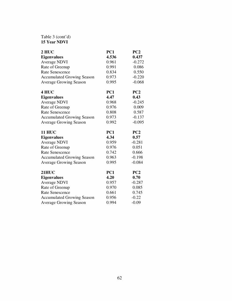
62
Table 3 (cont’d) 15 Year NDVI
2 HUC PC1 PC2 Eigenvalues 4.536 0.437 Average NDVI 0.961 -0.272 Rate of Greenup 0.991 0.086
Rate Senescence 0.834 0.550 Accumulated Growing Season 0.973 -0.220
Average Growing Season 0.995 -0.068
4 HUC PC1 PC2
Eigenvalues 4.47 0.43 Average NDVI 0.968 -0.245 Rate of Greenup 0.976 0.009
Rate Senescence 0.808 0.587 Accumulated Growing Season 0.973 -0.137
Average Growing Season 0.992 -0.095
11 HUC PC1 PC2
Eigenvalues 4.34 0.57 Average NDVI 0.959 -0.281 Rate of Greenup 0.976 0.051
Rate Senescence 0.742 0.666 Accumulated Growing Season 0.963 -0.198
Average Growing Season 0.995 -0.084
21HUC PC1 PC2
Eigenvalues 4.20 0.70
Average NDVI 0.957 -0.287 Rate of Greenup 0.970 0.085
Rate Senescence 0.661 0.745 Accumulated Growing Season 0.956 -0.22
Average Growing Season 0.994 -0.09
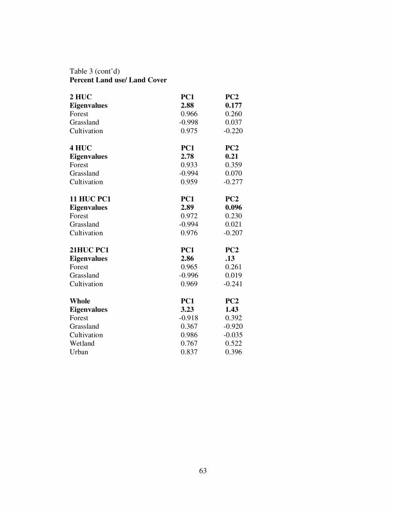
63
Table 3 (cont’d) Percent Land use/ Land Cover
2 HUC PC1 PC2
Eigenvalues 2.88 0.177 Forest 0.966 0.260 Grassland -0.998 0.037
Cultivation 0.975 -0.220
4 HUC PC1 PC2
Eigenvalues 2.78 0.21 Forest 0.933 0.359 Grassland -0.994 0.070
Cultivation 0.959 -0.277
11 HUC PC1 PC1 PC2
Eigenvalues 2.89 0.096 Forest 0.972 0.230 Grassland -0.994 0.021
Cultivation 0.976 -0.207
21HUC PC1 PC1 PC2
Eigenvalues 2.86 .13 Forest 0.965 0.261 Grassland -0.996 0.019
Cultivation 0.969 -0.241
Whole PC1 PC2
Eigenvalues 3.23 1.43
Forest -0.918 0.392 Grassland 0.367 -0.920
Cultivation 0.986 -0.035 Wetland 0.767 0.522
Urban 0.837 0.396

64
TABLE 4
Results of Pearson Product Moment Correlation. Mean fifteen-year NDVI, water quality, and fish community structure variables (diversity, fish community structure, trophic guild structure, invertebrate family richness, and EPT number (number of aquatic insects in the families within the orders of Ephemeroptera, Plecoptera and Trichoptera)) were reduced using principal component analysis (see Table 3; see Table 1 for descriptions of NDVI and LPMs). Results include Pearson Product Moment correlation r, p-value (*p<0.05, **p<0.01, ***p<0.001), and PC1(1) or PC2 (2) of dependent variables.
TP Diversity Fish Trophic Water δδδδ15
N Nutrients Invertebrate EPT
Community Guild Quality Family
Structure Richness
2-HUC
Start week NS NS NS NS -0.732* (2) NS NS NS NS
Start NDVI NS 0.860**(1) NS 0.977***(1) NS -0.920*** -0.861* NS (fish) (TP)
Max week NS NS NS NS 0.812* (1) NS
Max NDVI NS 0.717*(1) NS 0.834**(1) -0.720* (2) -0.922*** -0.811* NS NS (fish) (TP)
End Week NS NS NS NS NS NS NS NS NS
End NDVI NS NS NS NS NS NS NS NS NS
Rate of Green Up NS 0.723*(1) NS NS NS -0.737* NS 0.849** 0.723*
(fish) Rate of
Senescence NS -0.835**(1) NS NS NS 0.731* NS NS NS (fish)
Accumulated growing
season NS 0.844**(1) NS 0.962***(1) NS -0.987*** -0.918** 0.778* 0.826* (fish) (TP)
-0.715* (base)
Average growing s
season NS 0.833**(1) NS 0.960***(1) -0.756* (2) -0.971*** -0.896** 0.717* 0.768* (fish) (TP)
15 year PCA NS 0.849**(1) NS 0.979***(1) NS -0.974*** -0.888** 0.775* 0.804* (Fish) (TP)

65
Table 4 (cont’d)
TP Diversity Fish Trophic Water δδδδ15
N Nutrients Invertebrate EPT
Community Guild Quality Family
Structure Richness
4-HUC
Start week NS NS NS NS NS NS NS NS NS
Start NDVI NS -0.869*(1) -0.711*(1) 0.970***(1) NS -0.903** -0.844* NS NS (fish) (TP)
Max week NS NS NS NS 0.843** (1) NS NS NS NS
Max NDVI NS 0.816*(1) NS 0.911***(1) -0.744* (2) -0.949*** -0.831* NS 0.716* (fish) (TP)
End Week NS NS NS NS NS NS NS NS NS
End NDVI NS NS NS NS NS NS NS NS NS
Rate of Green Up NS 0.757*(1) NS NS NS -0.786* NS 0.943*** 0.863**
(fish) Rate of
Senescence NS -0.803*(1) NS NS NS NS NS NS NS
Accumulated Growing
Season NS 0.844**(1) NS 0.962***(1) -0.732* (2) -0.977** -0.947*** 0.742* 0.826* (fish) (TP)
-0.760* (base)
Average growing
season NS 0.844**(1) NS 0.968***(1) -0.759* (2) -0.955*** -0.900** NS 0.770* (fish) (TP)
15 year PCA NS 0.858* (1) NS 0.985***(1) -0.971*** -0.908** 0.759* 0.809* (fish) (TP)
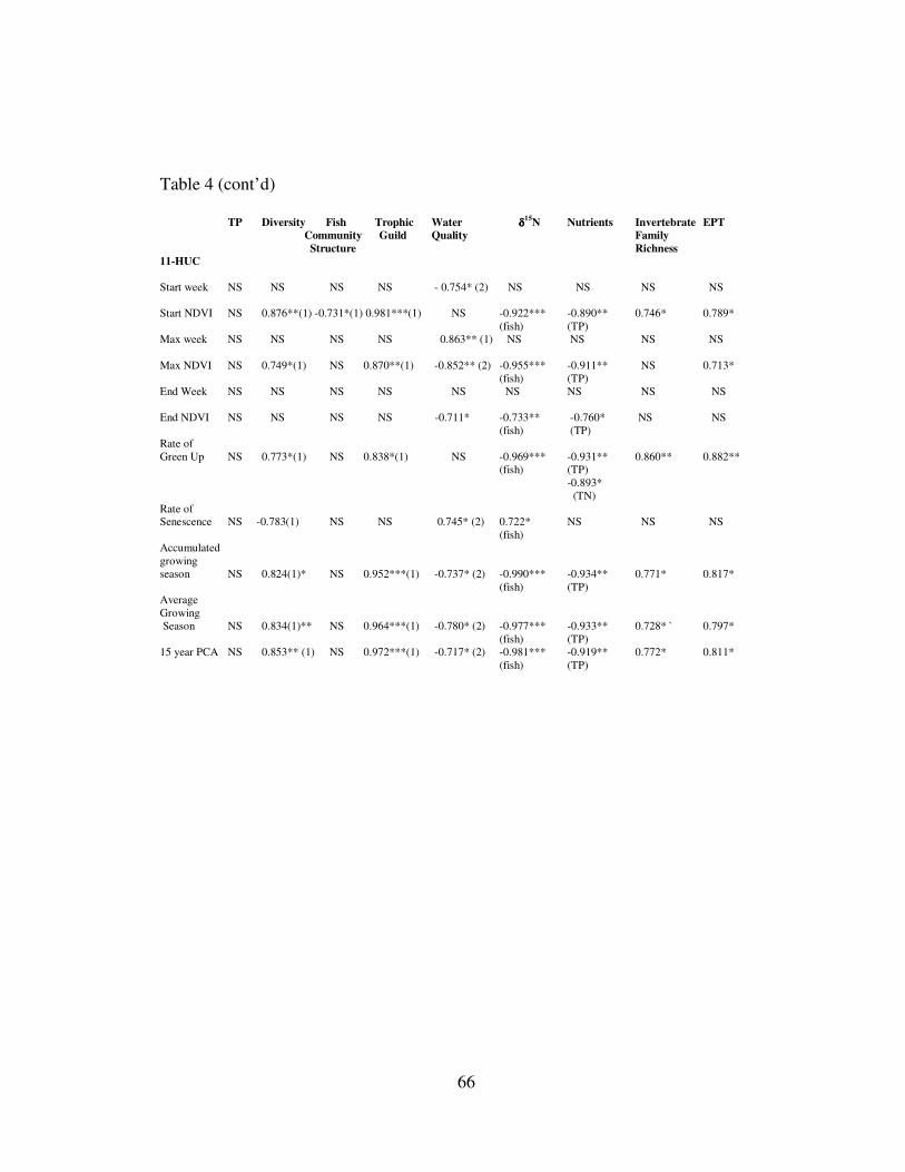
66
Table 4 (cont’d)
TP Diversity Fish Trophic Water δδδδ15
N Nutrients Invertebrate EPT
Community Guild Quality Family
Structure Richness
11-HUC
Start week NS NS NS NS - 0.754* (2) NS NS NS NS
Start NDVI NS 0.876**(1) -0.731*(1) 0.981***(1) NS -0.922*** -0.890** 0.746* 0.789*
(fish) (TP) Max week NS NS NS NS 0.863** (1) NS NS NS NS
Max NDVI NS 0.749*(1) NS 0.870**(1) -0.852** (2) -0.955*** -0.911** NS 0.713*
(fish) (TP) End Week NS NS NS NS NS NS NS NS NS
End NDVI NS NS NS NS -0.711* -0.733** -0.760* NS NS
(fish) (TP) Rate of
Green Up NS 0.773*(1) NS 0.838*(1) NS -0.969*** -0.931** 0.860** 0.882** (fish) (TP)
-0.893* (TN)
Rate of Senescence NS -0.783(1) NS NS 0.745* (2) 0.722* NS NS NS
(fish) Accumulated
growing season NS 0.824(1)* NS 0.952***(1) -0.737* (2) -0.990*** -0.934** 0.771* 0.817*
(fish) (TP) Average
Growing Season NS 0.834(1)** NS 0.964***(1) -0.780* (2) -0.977*** -0.933** 0.728* ` 0.797*
(fish) (TP) 15 year PCA NS 0.853** (1) NS 0.972***(1) -0.717* (2) -0.981*** -0.919** 0.772* 0.811*
(fish) (TP)

67
Table 4 (cont’d)
TP Diversity Fish Trophic Water δδδδ15
N Nutrients Invertebrate EPT
Community Guild Quality Family
Structure Richness
21-HUC
Start week NS 0.745*(1) NS NS NS NS NS NS NS
Start NDVI NS 0.883**(1) -0.734*(1) 0.979***(1) NS -0.918*** -0.911** 0.731* 0.796*
(fish) (TP) Max week NS NS NS NS 0.776*(1) NS NS NS NS
Max NDVI NS 0.769*(1) NS 0.863**(1) -0.850** (2) -0.954*** -0.911** NS NS
(fish) (TP) End Week NS NS 0.784*(1) NS 0.741* (1) NS NS NS NS
End NDVI NS NS NS NS -0.849**(2) -0.829* -0.883** NS NS
(fish) (TP) Rate of
Green Up NS NS NS 0.772*(1) NS -0.878** -0.847** 0.804* 0.760* (fish)
Rate of Senescence NS -0.855**(1) NS NS NS 0.745* NS NS NS
(fish) Accumulated
Growing Season NS 0.796*(1) NS 0.934***(1) -0.783*(2) -0.989***(fish) -0.952***(TP) 0.757* 0.815*
Average
Growing Season NS 0.852**(1) NS 0.955***(1) -0.793*(2) -0.978*** -0.940** 0.722* 0.795*
(fish) (TP) 15 year PCA NS 0.861** (1) NS `0.962***(1) -0.745* (2) -0.983*** -0.931** 0.756* 0.804*
(fish) (TP)

68
Table 4 (cont’d)
LPM
TP Diversity Fish Trophic Water δδδδ15
N Nutrients Invertebrate EPT
Community Guild Quality Family
Structure Richness
2 HUCs
TCA NS 0.760*41(1) -0.707*41(1) 0.975***41(1) 0.710*71(2) -0.875**41(f) -0.858*41(P) -0.732*82 NS -0.822*82(1) 0.908**(82)(f) 0.838*82(P)
NUMP NS 0.735*A(1) -0.721A(1) -0.828**82(1) NS 0.790*41(f) 0.842*41(P) -0.716*41 -0.727*82
0.807*82(f) 0.882**22(P) -0.807*82 -0.709*22 0.933*22(N)
MPS NS NS NS 0.921 ***41(1) 0.863*71(2) -0.854**41(f) -0.829*41(P) 0.708*41 0.770*41 -0.745* 82(1) -0.801* A(1) 0.743*71(f) 0.754*71(P) -0.711*82 -0.712*82
0.729*A(1) 0.887**82(f) 0.804*82(P)
ED NS 0.927***41(1) NS 0.783*41(1) 0.771*71(2) -0.828*41(f) 0.798*82(P) 0.765*41 0.734*41
-0.833**82(1) -0.957***82(1) 0.769**81(1) 0.935***82(f) -0.791*82 -0.805*82 -0.707*A(2) 0.737*82(b)
AWMSI NS 0.827* (1) -0.727*(1) NS NS NS NS NS NS
AWMPFD NS -0.795*(1) NS NS NS NS NS NS
IJI -0.806*(2) 0.720*(2) NS NS NS NS -0.773* -0.728*
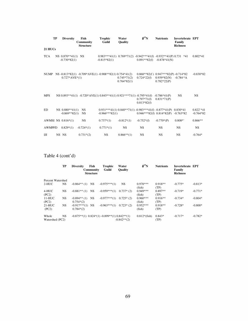
69
TP Diversity Fish Trophic Water δδδδ15
N Nutrients Invertebrate EPT
Community Guild Quality Family
Structure Richness
21 HUCs TCA NS 0.870**41(1) NS 0.983***41(1) 0.769*71(2) -0.942***41(f) -0.932**41(P) 0.731 *41 0.802*41
-0.730*82(1) -0.815*82(1) 0.891**82(f) -0.878*41(N)
NUMP NS -0.813*82(1) -0.709*AVE(1) -0.908**82(1) 0.754*41(2) 0.868**82(f ) 0.947***82(P) -0.714*82 -0.830*82 0.727*AVE*(1) 0.745*71(2) 0.724*22(f) 0.939*82(N) -0.784 *A
0.764*82(1) 0.782*22(P)
MPS NS 0.893**41(1) -0.720*AVE(1) 0.845**41(1) 0.921***71(1) -0.795*41(f) -0.786*41(P) NS NS 0.797*71(f) 0.831*71(P)
0.813*82(f)
ED NS 0.880**41(1) NS 0.931***41(1) 0.840**71(1) -0.983***41(f) -0.877*41(P) 0.830*41 0.822`*41 -0.869**82(1) NS -0.966***82(1) 0.946***82(f) 0.814*82(P) -0.763*82 -0.764*82
AWMSI NS 0.816*(1) NS 0.737*(1) -0.812*(1) -0.752*(f) -0.770*(P) 0.808*` 0.866**
AWMPFD 0.829*(1) -0.724*(1) 0.771*(1) NS NS NS NS NS
IJI NS NS 0.731*(2) NS 0.866**(1) NS NS NS -0.764*
Table 4 (cont’d)
TP Diversity Fish Trophic Water δδδδ15
N Nutrients Invertebrate EPT
Community Guild Quality Family
Structure Richness
Percent Watershed 2-HUC NS -0.864** (1) NS -0.975***(1) NS 0.978*** 0.918** -0.775* -0.813*
(fish) (TP) 4-HUC NS -0.881** (1) NS -0.959***(1) 0.737* (2) 0.949*** 0.897** -0.719* -0.771*
(PC2) (fish) (TP) 11-HUC NS -0.894** (1) NS -0.977***(1) 0.725* (2) 0.960*** 0.916** -0.734* -0.804*
(PC2) 0.754*(2) (fish) (TP) 21-HUC NS -0.917***(1) NS -0.963***(1) 0.723* (2) 0.952*** 0.918** -0.728* -0.800*
(PC2) 0.784*(2) (fish) (TP)
Whole NS -0.875**(1) 0.824*(1) -0.899**(1) 0.842**(1) 0.812*(fish) 0.843* -0.717* -0.782* Watershed (PC2) -0.842**(2) (TP)
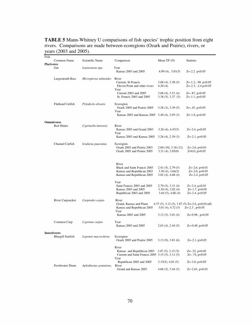
70
TABLE 5 Mann-Whitney U comparisons of fish species’ trophic position from eight rivers. Comparisons are made between ecoregions (Ozark and Prairie), rivers, or
years (2003 and 2005). Fish
Common Name Scientific Name Comparison Mean TP (N) Statistic
Piscivores Gar Lepisosteus spp. Year
Kansas 2003 and 2005 4.09 (4), 3.81(5) Z=-2.2 p<0.05
Largemouth Bass Micropterus salmoides River Current, St Francis 3.68 (4), 3.38 (5) Z=-1.2,-.98 p>0.05
Eleven Point and other rivers 4.20 (4) Z=-2.3, -2.4 p<0.05 Year
Current 2003 and 2005 3.68 (4), 3.51 (4) Z=-.87, p>0.05 St. Francis 2003 and 2005 3.38 (5), 3.37 (5) Z=-1.1, p>0.05
Flathead Catfish Pylodictis olivaris Ecoregion
Ozark 2005 and Prairie 2005 3.28 (3), 3.39 (5) Z=-.45, p>0.05 Year
Kansas 2003 and Kansas 2005 3.49 (4), 2.95 (3) Z=-1.8, p>0.05
Omnnivores
Red Shiner Cyprinella lutrensis River
Kansas 2003 and Grand 2003 3.26 (4), 4.47(5) Z=-2.4, p<0.05 Year
Kansas 2003 and Kansas 2005 3.26 (4), 2.39 (3) Z=-2.1, p=0.05
Channel Catfish Ictalurus punctatus Ecoregion Ozark 2003 and Prairie 2003 2.60 (10), 3.18 (12) Z=-2.6, p<0.01
Ozark 2005 and Prairie 2005 3.31 (4), 3.85(8) Z=0.0, p>0.05
River Black and Saint Francis 2003 2.41 (5), 2.79 (5) Z=-2.6, p<0.01
Kansas and Republican 2003 3.30 (4), 3.64(5) Z=-2.0, p>0.05 Kansas and Republican 2005 3.02 (4), 4.68 (4) Z=-2.4, p<0.05
Year
Saint Francis 2003 and 2005 2.79 (5), 3.31 (4) Z=-2.4, p<0.01 Kansas 2003 and 2005 3.30 (4), 3.02 (4) Z=-1.7, p>0.05
Republican 2003 and 2005 3.64 (5), 4.68 (4) Z=-2.4, p<0.05
River Carpsucker Carpiodes carpio River Grand, Kansas and Platte 4.37 (5), 3.12 (5), 1.87 (5) Z=-2.6, p<0.01(all)
Kansas and Republican 2005 3.01 (4), 4.72 (5) Z=-2.3 , p<0.05 Year
Kansas 2003 and 2005 3.12 (5), 3.01 (4) Z=-0.98 , p>0.05
Common Carp Cyprinus carpio Year Kansas 2003 and 2005 2.63 (4), 2.44 (5) Z=-0.49, p>0.05
Insectivores
Bluegill Sunfish Lepomis macrochirus Ecoregion Ozark 2005 and Prairie 2005 3.13 (9), 3.81 (6) Z=-2.1, p>0.05
River
Kansas and Republican 2003 3.07 (5), 3.15 (5) Z=-.52, p>0.05 Current and Saint Francis 2005 3.15 (5), 3.11 (5) Z=-.74, p=0.05
Year Republican 2003 and 2005 3.15(5), 4.03 (5) Z=-2.0, p<0.05
Freshwater Drum Aplodinotus grunniens, River Grand and Kansas 2003 4.66 (5), 3.44 (5) Z=-2.61, p<0.01

71
Table 5 (cont’d)
Time Kansas 2003 and 2005 3.44 (5), 3.27 (3) Z=-0.745, p>0.05
Golden Redhorse Moxostoma erythrurum River
Black and Current 2.51(5), 2.98(5) Z=2.6, p<0.01 Black and Eleven Point 2.51(5), 3.23(5) Z=2.6, p<0.01
Black and Saint Francis 2.51(5), 3.00(5) Z=2.6, p<0.01
Current and Eleven Point 2.98(5), 3.23 (5) Z=-2.2, p<0.05 Current and Saint Francis 2.98(5), 3.00 (5) Z=-.104, p>0.05
Year
Current 2003 and 2005 2.98 (5), 2.88 (5) Z=-.731, p>0.05 Saint Francis 2003 and 2005 3.00 (5), 2.99 (5) Z=-.104, p>0.05
Planktivore
Gizzard Shad Dorosoma cepedianum Ecoregion Ozark 2005 and Prairie 2005 2.85 (10), 3.58 (8) Z=-2.5, p<0.05
River Current and Saint Francis 2005 2.90 (5), 2.80 (5) Z=-0.94, p>0.05
Kansas and Republican 2005 3.13 (5), 4.34 (3) Z=-2.2. p<0.05
Emerald Shiner Notropis atherinoides Ecoregion Ozark and Prairie 2003 2.76 (11), 2.57 (10) Z=-0.423, p>0.05
River Black and Saint Francis 2003 2.49(5), 3.00 (4) Z=-2.4, p<0.05
Platte and Republican 2003 1.96 (5), 3.18 (5) Z=-2.6, p<0.01 Year (Ozarks)
Saint Francis 2003 and 2005 3.00 (4), 2.98 (5) Z=0.0, p>0.05
Herbivore Stoneroller Campostoma spp. River
Black and Current 2.45 (5), 2.39 (5) Z=-1.4, p>0.05 Black and Saint Francis 2.45 (5), 2.77 (5) Z=-1.4, p>0.05
Black and Eleven Point 2.45 (5),2.85 (5) Z=-2.0, p=0.05 Current and Eleven Point 2.39 (5), 2.85 (5) Z=-2.6, p<0.01
Current and Saint Francis 2.39 (5), 2.77 (5) Z=-2.6, p<0.01 Eleven Point and Saint Francis 2.85 (5), 2.77 (5) Z=-1.1 p>0.05
Invertebrate Predator Gomphidae River
Current and Eleven Point 2.09 (5), 2.13 (5) Z=-0.73, p>0.05 Saint Francis (from other Ozark rivers) 1.32 (5) Z=-2.6, p<0.01
Kansas and Republican 2005 1.66 (4), 3.03 (4) Z=-2.3, p<0.05 Time
Republican 2003 and 2005 2.23 (3), 3.03 (4) Z=-2.1, p>0.05
Ceoargionidae River
Platte and Republican 2003 2.37 (5), 2.75 (5) Z=-1.4, p>0.05 Kansas and Republican 2005 1.89 (3), 3.05 (5) Z=-2.2, p<0.05
Time Current 2003 and 2005 2.37 (5), 2.03 (4) Z=-2.4, p<0.05
Republican 2003 and 2005 2.75 (5), 3.05 (5) Z=-2.2, p<0.05
Invertebrate Omnivore
Orconectes spp. Ecoregion
Ozark 2005 and Prairie 2005 2.11 (6), 2.47 (7) Z=0.57, p>0.05 River
Current and Saint Francis 2003 2.10 (4), 1.65 (5) Z=-1.5, p>0.05 Kansas and Republican 2005 1.72 (3), 3.04 (4) Z=-2.1, p>0.05
Year Saint Francis 2003 and 2005 1.65 (5), 2.08 (4) Z=-1.7, p>0.05 Kansas 2003 and 2005 2.80 (5), 1.72 (3) Z=-2.2, p<0.05

72
TABLE 6 Maximum (from piscivorous fish) and mean trophic position of fish as calculated by Post 2002b. VZ TP calculated by Vander Zanden’s (1996) model. Mean TP without Post’s 2007 Lipid correction. Alpha from Post’s 2002 model for calculating trophic position.
River max TP mean TP VZ TP TP not lipid corrected Alpha
2003
Central Plains
Grand (a) 4.52(0.047) 4.42(0.071) Kansas (b) 3.79(0.097) 3.27(0.060) 3.75(0.059) 3.52(0.060) 0.29(0.028) Platte (c) 2.64(0) 2.18 (0.14) 2.06(0.14) 1.17(0.23) 1.33(0.23) Republican (a) 3.36(0.071) 3.36(0.069)
Ozark Highland
Black (d) 2.78(0.051) 2.61(0.038) 2.47(0.038) 2.19(0.060) 1.04(0.070) Current (e) 3.55(0.033) 3.15(0.061) 3.11(0.065) 3.09(0.058) 0.63(0.18)
Eleven Point (f) 3.93(0.066) 3.44(0.090) 3.85(0.086) 3.53(0.094) 0.096(0.019) St. Francis (e) 3.43(0.084) 3.08(0.052) 3.08(0.052) 3.08(0.052) 0.55(0.024)
2005
Central Plains Kansas (b) 3.49(0.18) 3.02(0.094) 3.24(0.093) 3.09(0.091) 0.30(0.10)
Republican(g) 4.43(0.14) 4.30(0.092)
Ozark Highland
Current (e) 3.51(0.13) 3.07(0.058) 3.01(0.057) 3.00(0.059) 0.84(0.14) St. Francis (e) 3.34(0.058) 3.10(0.036) 3.08(0.038) 3.07(0.036) 0.77(0.054)

73
TABLE 7 Landscape pattern metrics calculated using ArcGIS FRAGSTAT. Description of metrics in Table 1. 2-HUC Total Core Area Ave Number Ave Mean Edge AWMSI AWMPFD IJI
(Forest) of Patches Patch Size Density
Black 8547 160 9.76 18.3 5.33 1.196 54.3
Current 6088 114 8.24 17.9 4.53 1.174 44.5 Eleven Point 8306 75 16.53 12.8 3.37 1.158 44.4
Grand 502 87 6.11 12.8 3.33 1.159 53.2 Kansas 2188 87 7.04 14.1 3.55 1.163 48.6
Platte 284 44 4.49 18.7 2.64 1.134 53.3 Republican 177 91 8.75 15.0 3.54 1.176 48.7
Saint Francis 9916 79 14.29 11.2 3.28 1.160 45.5
21-HUC Total Core Area Ave Number Ave Mean Edge AWMSI AWMPFD IJI
(Forest) of Patches Patch Size Density
Black 128,736 1150 15.10 11.5 8.04 1.191 49.6 Current 126,523 1384 12.92 13.1 10.13 1.187 45.4
Eleven Point 114,972 1342 7.97 12.3 8.90 1.173 41.5 Grand 3158 767 6.93 13.0 3.62 1.170 55.7
Kansas 15,183 1396 6.35 15.6 3.94 1.169 56.8 Platte 6521 817 6.04 14.7 3.72 1.169 55.8
Republican 2403 893 11.24 11.7 6.45 1.170 47.1 Saint Francis 126882 1090 11.21 11.2 6.09 1.183 50.6

74
APPENDIX B. FIGURES
FIGURE 1. Watersheds sampled within the terrestrial ecoregion. Rivers are the Saint Francis (A), Black (B) Current (C), Eleven Point (D), Lower Grand (E); Platte (F), Kansas (G), and Republican (H) Rivers.

75
FIGURE 2.
Descriptions of NDVI vegetation phenology curve and metrics (based on graphs from Griffith et al. 2002a and Reed et al. 1994)

76
FIGURE 3. Percent land use of rivers from the Ozark and Prairie ecoregion. The lowest size subwatershed is 2 USGS Hydrologic Unit Code sub-watersheds above the sampling location are aggregated together. An aggregation of 2-21 HUCs are shown: (a) percent cultivation; (b) percent forest; (c) percent grassland. Ozark ecoregion rivers include the Black, Current, Eleven Point, and Saint Francis Rivers. Prairie ecoregion rivers include the Grand, Kansas, Platte, and Republican.
a). b).
Scale
2-HUC4-HUC
11-HUC21-HUC
WHOLE
Per
cen
t C
ult
ivat
ion
0
20
40
60
80
100
c). Scale
2-HUC4-HUC
11-HUC21-HUC
WHOLE
Per
cent
Fore
st
0
20
40
60
80
100
Scale
2-HUC4-HUC
11-HUC21-HUC
Whole
Per
cent
Gra
ssla
nd
0
20
40
60
80
100
Black River
Current River
Eleven Point River
Grand River
Kansas River
Platte River
Republican River
Saint Francis River

77
FIGURE 4. Normalized difference vegetation index (NDVI) phenology curves for eight rivers. Each data set is calculated from biweekly composites. Shown are subwatersheds consisting of : (a) 2 USGS HUCs and (b) 21 USGS HUCs.
a).
Week
4 6 8 10 12 14 16 18 20 22 24 26
ND
VI
0.2
0.3
0.4
0.5
0.6
0.7
0.8
0.9
Black River
Current River
Eleven Point River
Grand River
Kansas River
Platte River
Republican River
Saint Francis River
b).
Week
4 6 8 10 12 14 16 18 20 22 24 26
ND
VI
0.2
0.3
0.4
0.5
0.6
0.7
0.8
0.9
Black River
Current River
Eleven Point River
Grand River
Kansas River
Platte River
Republican River
Saint Francis River

78
FIGURE 5. Correlations between TP, diversity, and principal component factors.
Percent Watershed Land Use Principal Component Score 1
-1.5 -1.0 -0.5 0.0 0.5 1.0 1.5 2.0Div
ersi
ty
Pri
nci
pal
Co
mpo
nen
t F
acto
r S
core
1
-1.5
-1.0
-0.5
0.0
0.5
1.0
1.5
PC1 High percent of cultivation,
urban areas and wetland. Low percent of forest.
a.

79
Water Quality Principal Component Factor Scores
-2.0 -1.5 -1.0 -0.5 0.0 0.5 1.0 1.5 2.0Div
ersi
ty
Pri
nci
pal
Co
mpo
nen
t F
acto
r S
core
1
-1.5
-1.0
-0.5
0.0
0.5
1.0
1.5
2.0
PC1
PC2
PC1 High temperature, low dissolved oxygen
and high turbidity PC2
High conductivity High pH
b.
Diversity Principal Component Factors Scores
-1.5 -1.0 -0.5 0.0 0.5 1.0 1.5 2.0
Tro
ph
ic P
osi
tio
n
2.5
3.0
3.5
4.0
4.5
5.0
PC1
PC2
PC1 High fish species richness,
alpha diversity and Simpson’s Reciprocal D PC2 High fish abundance (N)
c.

80
Number of small fish
0 200 400 600 800 1000
Tro
ph
ic P
osi
tio
n
2.5
3.0
3.5
4.0
4.5
5.0
d.
Fish Community Proportion Principal Component Factor Scores
-2 -1 0 1 2 3
Tro
phic
Po
siti
on
2.5
3.0
3.5
4.0
4.5
5.0
PC1
PC2
PC1 High percent of Lepisosteus spp., Ictaluridae and Aplodinotus grunniens Low percent Catostomidae and Centarchidae.
PC2 Low percent Cyprinidae
e.

81
Trophic Guild Proportions Principal Component Factor Scores
-3 -2 -1 0 1 2
Tro
phic
Po
siti
on
2.5
3.0
3.5
4.0
4.5
5.0
PC1
PC2
PC1 High percent of Invertivores, Low percent of Omnivores.
PC2 Low percent of Herbivores. High percent of Planktivores
f.
Water Quality Principal Component Factor Scores
-2.0 -1.5 -1.0 -0.5 0.0 0.5 1.0 1.5 2.0
Tro
ph
ic P
osi
tio
n
2.5
3.0
3.5
4.0
4.5
5.0
PC1
PC2
PC1 High temperature, low dissolved oxygen and high turbidity
PC2 High conductivity High pH
g.

82
River Size Principal Component Factor Scores
-2 -1 0 1 2 3
Tro
phic
Posi
tion
2.5
3.0
3.5
4.0
4.5
5.0
PC1
PC2
PC1 High watershed area, dendritic length and dendritic density
PC2 High discharge
h.
Coeffecient of Variation of Discharge
50 100 150 200 250 300
Tro
phic
Po
siti
on
2.5
3.0
3.5
4.0
4.5
5.0
i.

83
FIGURE 6. Fish trophic structure calculated as proportion of each trophic guild to the number of fish caught. Samples collected in 2003.
River
Rep
ublic
an
Lower
Kan
sas
Lower
Gra
nd
Platte
(MO
)
Bla
ck
St. Fra
ncis
Cur
rent
Eleve
n Poi
nt
Pro
port
ion o
f to
tal
com
mu
nit
y
0.0
0.2
0.4
0.6
0.8
1.0
Planktivore
Herbivore
Invertivore
Omnivore
Piscivore

84
FIGURE 7. The δ15N and δ13C of fish and invertebrates caught within rivers. Bars represent one standard deviation. Rivers are the Black River (a), Current (b), Eleven Point River (c), Grand River (Missouri) (d), Kansas River (e), Platte River (f), Republican River (g), Saint Francis River (h), Kansas River 2005 (i),Republican River 2005(j), Saint Francis River 2005 (k), Current River 2005 (l).
-34 -32 -30 -28 -26 -24
5
6
7
8
9
10
11
12
13
Fish
Invertebrates
δ15Ν
a.
δ13C

85
-34 -33 -32 -31 -30 -29 -28 -27 -26
4
6
8
10
12
14
Fish
Invertebrates
b:
δ15Ν
δ13C
-36 -34 -32 -30 -28 -26 -24 -22 -20
2
4
6
8
10
12
14
Fish
Invertebrates
c:
δ13C
δ 15Ν

86
-26 -24 -22 -20 -18 -16 -14
6
8
10
12
14
16
18
20
Fish
Invertebrates
e.
δ13C
δ15Ν
-34 -32 -30 -28 -26 -24 -22
2
4
6
8
10
12
14
16
18
Fish
Invertebrates
d.
δ13C
δ15Ν

87
-28 -26 -24 -22 -20 -18
6
8
10
12
14
16
18
20
22
Fish
Invertebrates
f.
δ13C
δ15Ν
-34 -32 -30 -28 -26 -24 -22
10
12
14
16
18
20
Fish
Invertebrates
g.
δ13C
δ15Ν

88
-32 -31 -30 -29 -28 -27 -26 -25 -24
δ15Ν
4
6
8
10
12
14
16
Fish
Invertebrates
h.
δ13C
-32 -30 -28 -26 -24 -22 -20
6
8
10
12
14
16
18
20
Fish
Invertebrates
i.
δ13C
δ15Ν

89
-30 -29 -28 -27 -26 -25 -24 -23 -22
δ15Ν
6
8
10
12
14
16
18
20
Fish
Invertebrates
j.
δ13C
-34 -32 -30 -28 -26 -24
6
7
8
9
10
11
12
13
Fish
Invertebrates
k.
δ13C
δ15Ν

90
-36 -35 -34 -33 -32 -31 -30 -29 -28
4
6
8
10
12
14
Fish
Invertebrates
δ13C
δ15Ν
l.

91
FIGURE 8. The mean trophic position of fish within trophic guilds. Bars represent one standard error.
Top PiscivoreInvertivore
OmnivorePlanktivore
Herbivore
Mea
n T
rop
hic
Posi
tio
n
0
1
2
3
4
5
Ozark Highland 2003
Central Prairie 2003
Ozark Highland 2005
Central Prairie 2005

92
FIGURE 9 Proportion of the number of fish caught within each fish family by the number of fish caught. Fish collected in 2003.
River
Rep
ublic
an
Lower
Kan
sas
Lower
Gra
nd
Platte
(MO
)
Bla
ck
St. Fra
ncis
Cur
rent
Eleve
n Poi
nt
Pro
port
ion
of
Fis
h F
amil
y
0.0
0.2
0.4
0.6
0.8
1.0

93
FIGURE 10. Percent of fish species within the Cyprinidae family excluding Cyprinus
carpio. Rivers are the Republican River (a), Kansas River (b), Grand River (c), Platte River (d), Black River (e), Saint Francis River (f), Current River (g), Eleven Point River (h).

94
a.
Red Shiner
Emerald Shiner

95
b.
Red Shiner
Emerald Shiner
Sand Shiner
Suckermouth Minnow
Bullhead Minnow
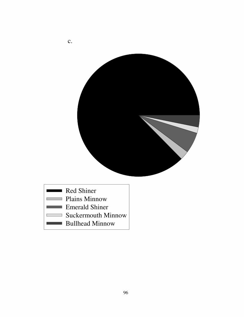
96
c.
Red Shiner
Plains Minnow
Emerald Shiner
Suckermouth Minnow
Bullhead Minnow
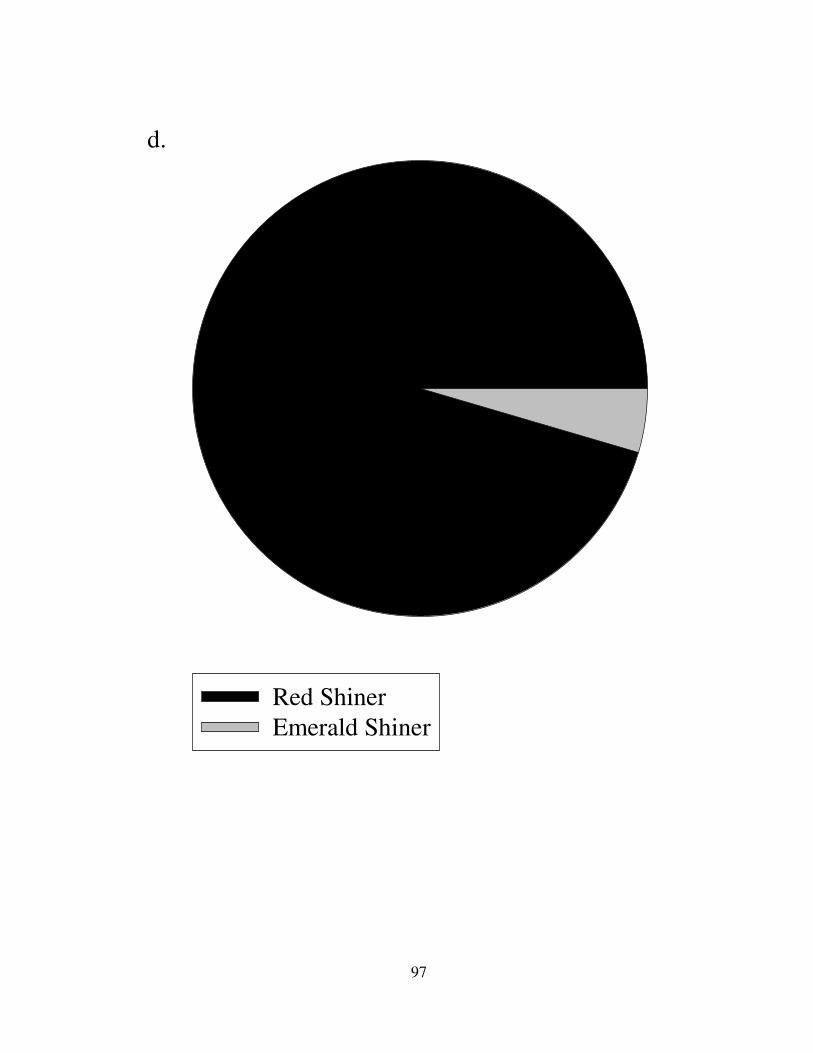
97
d.
Red Shiner
Emerald Shiner

98
e.
Central Stoneroller
Whitetail Shiner
Blacktail Shiner
Mississippi Silvery Minnow
Emerald Shiner
Bigeye Shiner
Wedgespot Shiner
Sabine Shiner
Bluntnosed Minnow
Bullhead Minnow
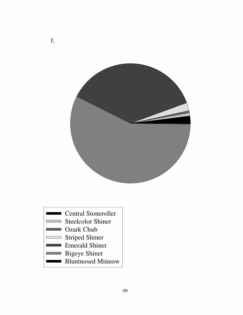
99
f.
Central Stoneroller
Steelcolor Shiner
Ozark Chub
Striped Shiner
Emerald Shiner
Bigeye Shiner
Bluntnosed Minnow

100
g.
Largescale Stoneroller
Central Stoneroller
Whitetailed Shiner
Ozark Chub
Striped Shiner
Bleeding Shiner
Hornyhead Chub
Bigeye Chub
Emerald Shiner
Bigeye Shiner
Wedgespot Shiner
Ozark Minnow
Rosyfaced Minnow
Telescope Shiner
Bluntnosed Minnow

101
Largescale Stoneroller
Central Stoneroller
Striped Shiner
Bleeding Shiner
Hornyhead Chub
Bigeye Chub
Emerald Shiner
Ozark Minnow
Rosyfaced Minnow
Telescope Shiner
Bluntnose Minnow
Bullhead Minnow
h.

102
TABLE i. Sizes of watersheds
Sizes of extent 2-HUC (ha) 21-HUC (ha) Whole Watershed (ha)
Black 17,362.53 204,158.70 311,291.11 Current 12,469.05 212,572.89 531,661.76 Eleven Point 12,824.64 256,135.69 256,467.34 Grand 15,078.78 130,128.12 1,963,263.39 Kansas 15,435.63 193,398.30 3,606,287.87 Platte 4397.31 119,286.63 614,444.69
Republican 14,968.62 218,139.48 6,385,525.10 Saint Francis 14,542.38 216,620.55 242,813.26

103
FIGURE ii: Trophic position of species caught.
________________________________________________________________________
Common name N Scientific name Trophic Guild Trophic Position
Black crappie 4 Pomoxis nigromaculatus Piscivore 2.89 Bleeding shiner 5 Luxilus zonatus Invertivore 3.01
Bluegill sunfish 25 Lepomis macrochirus Invertivore 3.29 Bluntnose shiner 4 Pimephalus notatus Omnivore 2.90
Channel catfish 34 Ictalurus punctatus Omnivore 3.18 Common carp 11 Cyprinus carpio Omnivore 2.78
Drum 14 Aplodinotus grunniens Invertivore 3.75 Dusky darter 3 Percina sciera Invertivore 2.62
Emerald shiner 26 Notropis antherinoides Planktivore 2.73 Fantailed darter 1 Etheostoma flabellare Invertivore 2.59
Flathead catfish 13 Pylodictis olivaris Piscivore 3.48 Gar (Long and short) 11 Lepisosteus spp. Piscivore 4.11
Gizzard shad 20 Dorosoma cepedianum Planktivore 3.15 Golden Redhorse 30 Moxostoma erythrurum Invertivore 2.93
Goldeneye 3 Hiodon alosoides Invertivore 4.33 Green sunfish 5 Lepomis cyanellus Piscivore 3.36
Hornyhead chub 1 Nocomis biguttatus Omnivore 3.02 Largemouth bass 23 Micropterus salmoides Piscivore 3.64
Logperch 21 Percina caprodes Invertivore 2.94 Longear sunfish 9 Lepomis megalotis Invertivore 3.04
Mississippi silvery minnow 3 Hybognathus nuchalis Herbivore 3.07
Mosquito fish 2 Gambusia affinis Invertivore 2.88 Rainbow darter 1 Etheostoma caeruleum Invertivore 3.11
Red shiner 14 Cyprinella lutrensis Omnivore 3.46 Redear sunfish 3 Lepomis microlophus Invertivore 3.05
River carpsucker 24 Carpiodes carpio Omnivore 3.43 Rock bass 4 Ambloplites rupestris Piscivore 3.53
Rosyface shiner 2 Notropis rubellus Insectivore 3.01 Shadow bass 4 Ambloplites ariommus Piscivore 3.66
Smallmouth bass 12 Micropterus dolomieu Piscivore 3.68 Spotted bass 15 Micropterus punctulatus Piscivore 3.22
Spotted sucker 2 Minytrema melanops Invertivore 3.34 Stoneroller 20 Campostoma spp. Herbivore 2.62
White Crappie 10 Poxomis annularis Piscivore 4.14