Landscape connectivity for bobcat (Lynx rufus) and lynx ... · Supporting Information (S1 Table)....

RESEARCH ARTICLE

Landscape connectivity for bobcat (Lynx rufus)

and lynx (Lynx canadensis) in the Northeastern

United States

Laura E. Farrell1¤a*, Daniel M. Levy2¤b, Therese Donovan3, Ruth Mickey4, Alan Howard5,

Jennifer Vashon6, Mark Freeman3, Kim Royar7, C. William Kilpatrick1

1 Department of Biology, University of Vermont, Burlington, Vermont, United States of America,

2 Rubenstein School of Environment and Natural Resources, University of Vermont, Burlington, Vermont,

United States of America, 3 U.S. Geological Survey, Vermont Cooperative Fish and Wildlife Research Unit,

Rubenstein School of Environment and Natural Resources, University of Vermont, Burlington, Vermont,

United States of America, 4 Department of Mathematics and Statistics, University of Vermont, Burlington,

Vermont, United States of America, 5 Statistical Consulting Clinic, University of Vermont, Burlington,

Vermont, United States of America, 6 Maine Department of Inland Fisheries and Wildlife, Bangor, Maine,

United States of America, 7 Vermont Fish and Wildlife Department, Springfield, Vermont, United States of

America

¤a Current address: Otter Ridge Consulting LLC, Monkton, Vermont, United States of America

¤b Current address: GIS Consultant, Waterbury, Vermont, United States of America

* [email protected]

Abstract

Landscape connectivity is integral to the persistence of metapopulations of wide ranging

carnivores and other terrestrial species. The objectives of this research were to investigate

the landscape characteristics essential to use of areas by lynx and bobcats in northern New

England, map a habitat availability model for each species, and explore connectivity across

areas of the region likely to experience future development pressure. A Mahalanobis dis-

tance analysis was conducted on location data collected between 2005 and 2010 from 16

bobcats in western Vermont and 31 lynx in northern Maine to determine which variables

were most consistent across all locations for each species using three scales based on

average 1) local (15 minute) movement, 2) linear distance between daily locations, and 3)

female home range size. The bobcat model providing the widest separation between used

locations and random study area locations suggests that they cue into landscape features

such as edge, availability of cover, and development density at different scales. The lynx

model with the widest separation between random and used locations contained five vari-

ables including natural habitat, cover, and elevation—all at different scales. Shrub scrub

habitat—where lynx’s preferred prey is most abundant—was represented at the daily dis-

tance moved scale. Cross validation indicated that outliers had little effect on models for

either species. A habitat suitability value was calculated for each 30 m2 pixel across Ver-

mont, New Hampshire, and Maine for each species and used to map connectivity between

conserved lands within selected areas across the region. Projections of future landscape

change illustrated potential impacts of anthropogenic development on areas lynx and bob-

cat may use, and indicated where connectivity for bobcats and lynx may be lost. These

PLOS ONE | https://doi.org/10.1371/journal.pone.0194243 March 28, 2018 1 / 25

a1111111111

a1111111111

a1111111111

a1111111111

a1111111111

OPENACCESS

Citation: Farrell LE, Levy DM, Donovan T, Mickey

R, Howard A, Vashon J, et al. (2018) Landscape

connectivity for bobcat (Lynx rufus) and lynx (Lynx

canadensis) in the Northeastern United States.

PLoS ONE 13(3): e0194243. https://doi.org/

10.1371/journal.pone.0194243

Editor: Jesus E. Maldonado, Smithsonian

Conservation Biology Institute, UNITED STATES

Received: June 16, 2017

Accepted: February 27, 2018

Published: March 28, 2018

Copyright: This is an open access article, free of all

copyright, and may be freely reproduced,

distributed, transmitted, modified, built upon, or

otherwise used by anyone for any lawful purpose.

The work is made available under the Creative

Commons CC0 public domain dedication.

Data Availability Statement: The data on bobcat

locations used in these analyses is uploaded into

Supporting Information (S1 Table). The lynx

telemetry data are sensitive as this is a threatened

species, and research was conducted completely

on private lands. To protect relationships with

landowners and maintain future access to

private lands it is necessary to limit availability of

the data to upon request. Data requests will be

considered on a case by case basis, and should

be sent to Canada Lynx Biologist at Maine

Department of Inland Fisheries and Wildlife

https://doi.org/10.1371/journal.pone.0194243

http://crossmark.crossref.org/dialog/?doi=10.1371/journal.pone.0194243&domain=pdf&date_stamp=2018-03-28








https://creativecommons.org/publicdomain/zero/1.0/

https://creativecommons.org/publicdomain/zero/1.0/

projections provided a guide for conservation of landscape permeability for lynx, bobcat,

and species relying on similar habitats in the region.

Introduction

Forest cover across the Northeastern United States has increased since the early nineteenth

century as agricultural land has been abandoned. Populations of native carnivores have recov-

ered in response to increased habitat. For example, a breeding population of lynx (Lynx cana-densis) was absent from the region for decades but became reestablished naturally in Maine in

1999 [1], and more recently in New Hampshire [2], and Vermont [3]. Anthropogenic growth

is now reversing the 150-year increase in habitat and is projected to continue, increasing habi-

tat fragmentation and adding barriers to wildlife movement [4,5]. Long–term conservation of

wide–ranging species depends on maintaining landscapes in which both local daily move-

ments and longer inter-territorial dispersal events are possible [6,7]. Wide–ranging species

such as bobcat (Lynx rufus) and lynx (Lynx canadensis) rely on connective habitat to facilitate

seasonal range-shifts between heavily used core areas, as well as longer–distance movements

such as dispersal that link subpopulations and permit gene flow [1, 8, 9]. Dispersal distances

from natal ranges of up to 182 km for bobcat and 1100 km for lynx [10, 11], emphasize the

value of regional-scale conservation strategies.

Setting such strategies presents three major challenges. First, species have differing habitat

requirements that may require unique conservation solutions. Bobcats use broader landscape

characteristics including natural habitats, riparian areas, edge, and natural cover in areas of

moderate human use [12–14], but avoid areas of high human activity [15, 16]. Lynx are tightly

tied to boreal forest and shrub scrub (shrub < 5 m tall > 20% of canopy), as these are favored

habitat of their main prey, the snowshoe hare (Lepus americanus) [11]. Second, each species

cues into certain habitats for food acquisition, denning, or travel at different scales [17–22].

The scale at which variables are examined can determine what scales are most important to

utilization of resources, and influence the ability to accurately predict effects of habitat frag-

mentation on a particular species [23–25]. Thus, for effective conservation linkage strategies,

the interactions of multiple habitat variables at a range of spatial scales should be investigated

for each species [26–29]. And third, there is a need to map the amount and distribution of suit-

able habitat and the functional ability of the landscape to connect populations at a regional

scale to aid decision making [30].

As change to the Northeastern landscape intensifies in order to accommodate a greater

human population, maintaining ecosystem processes such as dispersal of wide ranging mam-

mals depends on identifying networks of connective habitat linking high quality core areas.

Efforts to create connectivity maps have been achieved for bobcats in New Hampshire and

lynx in the Rocky Mountains, and sub home-range scales have been investigated for pumas,

but corridor models using resource selection methods may not best predict landscape use [31–

35]. Regional connectivity models where scaled variables are not modeler selected, but instead

selected by distilling appropriate variables from locations, are lacking for lynx and bobcat in

the Northeast. A pragmatic connectivity assessment will not only consider the spatial distribu-

tion of habitats across a landscape in the current time, but can also predict its effectiveness as

landscapes change in the future. Identifying habitat and connective linkage areas, and deter-

mining how these may withstand development pressure, will help planners implement land

use strategies that will facilitate both human and wildlife needs through landscape changes.

Lynx and bobcat landscape connectivity


(http://www.maine.gov/ifw/about/contact/email.

html). All other relevant data are within the paper

and its Supporting Information files.

Funding: This work was supported by the US EPA

STAR Fellowship (https://cfpub.epa.gov/ncer_

abstracts/index.cfm/fuseaction/display.

abstractDetail/abstract/7582/report/0), F5F21809

to LF; and the Lindbergh Foundation (http://

lindberghfoundation.org/) to LF. The funders had

no role in study design, data collection and

analysis, decision to publish, or preparation of the

manuscript.

Competing interests: The authors have declared

that no competing interests exist.


http://www.maine.gov/ifw/about/contact/email.html

http://www.maine.gov/ifw/about/contact/email.html

https://cfpub.epa.gov/ncer_abstracts/index.cfm/fuseaction/display.abstractDetail/abstract/7582/report/0



http://lindberghfoundation.org/

http://lindberghfoundation.org/

Here, we used a partitioned Mahalanobis Distance Squared analysis (D2) to derive a habitat

suitability model for lynx and bobcat and map suitability across the Northeastern U.S. based

on GPS location data and the spatial covariates that are associated with each location. The D2

approach is a Principal Components Analysis (PCA), but rather than focusing on components

that explain the variation among locations, it reveals the habitat components that are most

similar across all locations; these represent the minimum habitat requirements for each species

and can be scored on a pixel-by-pixel basis [36]. These minimal habitat requirements are

assumed to identify all usable areas, including movement and dispersal habitat. Our objectives

were to: 1) use the D2 approach [36, 37] to identify the landscape characteristics, at biologically

relevant spatial scales, that are consistently used by known populations of lynx and by bobcat

in northern New England, and use the most highly validated model for each species to map a

movement suitability value for each 30 m2 pixel across Vermont, New Hampshire and Maine;

2) use the D2 model for each species to identify current connectivity (linked areas conducive to

movement) across subportions of the region by developing cost-distance based landscape con-

ductivity maps—including an area recently recolonized by unstudied lynx, and 3) estimate the

persistence of connectivity into the future in areas most likely to experience increased anthro-

pogenic pressure.

Methods

Study area

The regional area of analyses encompassed the states of Vermont (VT), New Hampshire (NH)

and Maine (ME), an area of 132,313 km2 (Fig 1). Empirical data for bobcat were collected in

northwestern Vermont, from the Champlain Valley lowlands eastward into the north central

Green Mountains, with Lake Champlain forming the western boundary. Temperatures in the

Champlain Valley are moderated by Lake Champlain; average daily highs range from over

21˚C in July to -11˚C in January. Summer temperatures in the mountains are often 6.7˚C

cooler [38]. Elevation ranged from 29 m at the edge of Lake Champlain to 1,245 m on top of

Camel’s Hump Mountain [38]. The 2,997 km2 study area, including portions of Chittenden,

Lamoille, Addison, and Washington Counties, contained a range of natural habitats inter-

spersed with rural agricultural and more densely developed areas [39]. Lowland forests were

predominantly hardwood; softwoods increased with elevation into the Green Mountains [38].

Road density in the bobcat study area ranged from 0 to between 0.84 linear km/ km2 and 9.36

km/ km2 [40], while human density in the Champlain Basin averaged 23.5 people/km2 [41].

Empirical lynx data were collected from a 19,875 km2 area, primarily in the Musquacook

lakes region of northwestern Maine (Fig 1). Average daily highs ranged from 24 C in July to -7

in January [42]. Elevation ranged between 250 and 550 m over rolling hills and wide valleys. A

matrix of spruce-fir forest was interspersed with lowland spruce-tamarack-cedar forests and

hardwood dominated ridges. Much of the area was clear cut in the 1980s, leading to extensive

areas of regenerating forest in the 1990s. Although road density is relatively high (~100km/

100km2), these dirt roads were used primarily for wood extraction and most were not main-

tained. Human density was 0 in the majority of the lynx study area, as activity was limited to

seasonal camps and logging operations [20]. One lynx (L114) made a long range movement

into the area around Bangor, ME, where road densities of well-travelled roads are high, and

human density exceeds 2,500/km2.

Location data

Bobcat GPS radio–collar locations were provided by the Vermont Cooperative Fish and Wild-

life Research Unit from a study conducted between 2005 and 2008 [39] (S1 Table). Lynx GPS




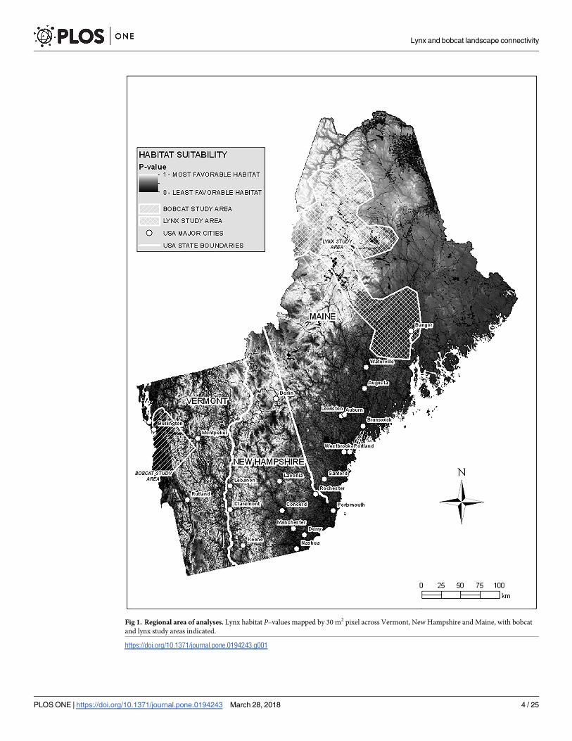
Fig 1. Regional area of analyses. Lynx habitat P–values mapped by 30 m2 pixel across Vermont, New Hampshire and Maine, with bobcat

and lynx study areas indicated.

https://doi.org/10.1371/journal.pone.0194243.g001





radio–collar locations were collected by Maine Department of Inland Fisheries and Wildlife

between 2005 and 2010 during a study that started in 1999 [20, 43]. Modeling was done from

these data.

GPS radio–collar locations were taken at regular intervals 24 hours a day. The full range of

locations were used to incorporate less frequently used habitats such as those used by individu-

als moving across longer distances. Locations from each cat were edited to 4 hours apart. We

balanced available data per cat with activity patterns to maximize independence, time between

locations and available data. There may be autocorrelation of some resting locations, though

both species move throughout the day depending on climate and daylight hours, and consis-

tency of use of certain habitats for both species underscores the importance of specific land-

scape variables. A maximum of 200 points were taken from each collar to minimize weighting

of data (S2 and S3 Tables). It was assumed that telemetry error for the ATS G2004 (Advanced

Telemetry Systems, Isanti MN), Lotek 3300S (Lotek Wireless Inc., Newmarket, Ontario) and

Sirtrack1 (Hawkes Bay, New Zealand) collars used was absorbed within the 30 m pixels and

the buffers around each location used in this analysis (T. Garin, Advanced Telemetry Systems,

pers. com.) [44, 45].

Lynx were found to be recolonizing New Hampshire after modeling but during the map-

ping phase of this study, and we took the opportunity to explore how the lynx population may

be recolonizing parts of its historic range. A connectivity map was produced using, instead of

core habitat blocks, 142 uncollared lynx locations from 2006 through 2011, verified by the US

Fish and Wildlife Service and state wildlife departments using photos, tracks and observations.

Selection of variables

The association of bobcat and lynx occurrences with 39 variables was evaluated across three

scales, each described by a map layer (Table 1, S1 Methods). Variables were selected to

describe: 1) fragmentation features such as edge, availability of cover, and patch size, 2) basic

landscape features including availability of water, elevation, slope, and slope aspect, 3) density

of anthropogenic features such as roads and urban areas, 4) density of habitat types and cover.

Maps used to construct variable layers included the 2006 National Land Cover Database

(NLCD), the National Elevation Dataset (NED), the National Hydrography Dataset, and the

National Transportation Dataset. The Landscape Fragmentation Tool v2.0 for ArcMAP 9.3

[46] was used to produce fragmentation associated layers. All mapping functions were con-

ducted at 30 m resolution in ArcMap 9.3 or ArcMap 10 (Esri, Redlands, CA).

The density of habitat variables was examined at three scales (local distance, daily distance

[44], and female home range size) by performing neighborhood analyses on binary variable

layers in ArcMap 9.3.1 [47]. A local scale with a 60 m radius was used because it is the average

distance a bobcat would travel in about 15 minutes [48], and captured smaller interspersed

habitat patches. The linear daily distance scale of 1.6 km diameter (810 m radius) was used for

bobcats [49, 50], and 3 km for lynx (1500 m radius) [51–53]. Female bobcats in VT and lynx

in ME have similar average home range sizes (22.9 km2 and 25.7 km2 respectively) [39, 43].

These were averaged to establish a home range scale covering 24.3 km2 (2790 m radius), under

the premise that male ranges encompass female ranges [54–56].

Topographic features are localized in many areas, including the Champlain Valley, and

would not have been as informative over larger neighborhoods. To provide greater definition

of topography, smaller scales with 90 m, 150 m and 270 m radii were arbitrarily chosen to eval-

uate slope, sin aspect, and cosine aspect. Elevation data were taken at location points only.

Values for each variable (map layer) were extracted from under radio-telemetry locations.

The most consistent variables within each species dataset (coefficient of variation, CV� 1)




Table 1. Map layers.

Scale Local Daily distance Home range Topographic

Radius of neighborhood analysis (in meters) 60 810 Bobcat 1500 Lynx 2790 90 150 270

Agricultural (ag)–includes pasture, hay and cultivated crops 1 2 3 4

Grasslands—grassland herbaceous, emergent herbaceous wetlands 5 6 7 8

Coniferous forest 9 10 11 12

Deciduous forest 13 14 15 16

Mixed forest 17 18 19 20

Shrub scrub 21 22 23 24

Woody wetlands 25 26 27 28

Developed open and low—developed open space, developed low intensity 29 30 31 32

Developed medium and high—developed medium intensity, developed high intensity 33 34 35 36

Forest cover—coniferous forest, deciduous forest, mixed forest 37 38 39 40

All cover—shrub scrub, woody wetlands, coniferous forest, deciduous forest, mixed forest 41 42 43 44

Patch—a small area of cover habitat surrounded by non-forested land cover 45 46 47 48

Ecotone/edge—the boundary of cover within 30 meters of open habitat 49 50 51 52

Small area of cover–< 250 acres (<1.01 km2) 53 54 55 56

Medium area of cover– 250–500 acres (1.01–2.02 km2) 57 58 59 60

Large area of cover–> 500 acres (>2.02 km2) 61 62 63 64

Stream River edge (km/km2) 65 66 67 68

Waterbody edge (km/km2)–streams, rivers, lakes and ponds 69 70 71 72

Roads class1 and 2 (km/km2) 73 74 75 76

Roads class 3 (km/km2) 77 78 79 80

Euclidean distance to stream river edge 81

Euclidean distance to waterbody edge 82

Euclidean distance to cover 83

Euclidean distance to class 1 and 2 roads 84

Euclidean distance to class 3 roads 85

Undeveloped (includes ag. areas) 86

Natural habitat (excludes devel & ag.) 87

Water_within100m 88

Water_within150m 89

Water_within300m 90

Cover_within100m 91

Cover_within150m 92

Cover_within300m 93

CoverEdge_200m –edge 100 meters inside and outside of forest (200m width total) 94

CoverEdge_300m –edge 150 meters inside and outside of forest (300m width total) 95

Elevation (location only) 96

Slope 97 98 99 100

Aspect sin 101 102 103 104

Aspect cosine 105 106 107 108

Map number for each variable, at scales of evaluation. Raster variables were evaluated by number of pixels within the scaled neighborhood buffer, and converted to

percentages for interpretation. Line densities were calculated for linear features (i.e. water and roads). Daily distance data for bobcats was taken from within an 810 m

radius, and for lynx within a 1500 m radius.

https://doi.org/10.1371/journal.pone.0194243.t001





were preselected and sets of uncorrelated variables were analyzed. Preselection reduced the

total variables to 31 for bobcat and 35 for lynx Mahalanobis distance analyses (Table 2).

Objective 1: Principal components analysis, partitioned Mahalanobis distance analysis

and mapping of movement suitability for each pixel. For each species, sets of the selected

variables were analyzed using principal components analysis (PCA), which describes increas-

ing amounts of variation within the dataset with a set of linear equations. For each PCA analy-

sis, we were interested in the component that described the least amount of variation (i.e.,

Table 2. Selected variables for bobcat and lynx models.

Bobcat variables Lynx variables

# Name CV Correlations # Name CV Correlations

2 Agricultural_810 0.676 15 Deciduous forest_1500 0.793 a

4 Agricultural_2790 0.522 c- 16 Deciduous forest_2790 0.606 a

12 Coniferous_2790 0.646 19 Mixed forest_1500 0.328 b

14 Deciduous_810 0.747 20 Mixed forest_2790 0.243 b

16 Deciduous_2790 0.530 d,e 23 �Shrubscrub_1500 0.589 c

24 Shrubscrub_2790 0.591 24 Shrubscrub_2790 0.521 c, d-

28 Wooded wetland_2790 0.589 27 Wooded wetlands_1500 0.831

50 Ecotone edge_810 0.439 28 Wooded wetlands_2790 0.593

52 �Ecotone edge_2790 0.297 40 All forest_2790 0.211 d-

56 Small Area Cover_2790 (<250 acres) 0.607 41 All cover_6 0.134 e

30 Development low_810 0.962 43 All cover_1500 0.078 f,g

32 Development low_2790 0.702 44 All cover_2790 0.063 h

40 All Forest cover habitats_2790 0.531 b,e 52 Ecotone edge_2790 0.579 i-

41 All cover habitats_60 0.645 a 61 Large area of cover_60 (> 500 acres) 0.219 e

44 All cover habitats_2790 0.446 b,c-,d 63 Large area of cover_1500 (> 500 acres) 0.097 f,j

46 Patch_810 0.855 64 Large area of cover_2790 (> 500 acres) 0.077 g,h,i -,j

48 Patch_2790 0.424 67 Stream or river edge_1500 (km/km2) 0.503

76 Class1 and 2 roads_2790 1.000 68 Stream or river edge_2790 (km/km2) 0.346

78 Class3 roads_810 0.773 71 Waterbody edge_1500 (km/km2) 0.428

80 Class3 roads_2790 0.447 72 Waterbody edge_2790 (km/km2) 0.300

85 Distance to class 3 road 0.803 79 Class3 roads_1500 (km/km2) 0.760 k

86 �Undeveloped_60 0.109 80 Class3 roads_2790 (km/km2) 0.616 k

87 Natural habitat_60 0.588 a 81 Distance to stream or river 0.824 l

89 Water within 150m_60 0.877 82 Distance to waterbody edge 0.841 l

90 �Water within 300m_60 0.499 84 Distance to class 1 and 2 roads 0.171

91 Cover within 100m_60 0.334 f 86 Undeveloped_60 0.027

92 Cover within 150m_60 0.228 f 87 �Natural habitat_60 0.031

93 �Cover within 300m_60 0.094 91 Cover within 100m_60 0.038

94 Cover_edge_100mIn_100Out_60 0.789 g 92 Cover within 150m_60 0.031

95 �Cover_edge_150mIn_150Out_60 0.595 g 93 �Cover within 300m_60 0.015

96 Elevation 0.785 96 �Elevation 0.151

97 Slope_60 0.666 m,n,o

�Final model 98 Slope_90 0.624 m,p,q

99 Slope_150 0.559 n,p,r

100 �Slope_270 0.473 o,q,r

Selected variables for bobcat and lynx models with coefficients of variation (CV). Starred variables are contained within the final model for each species. Sets of highly

correlated variables (rho>0.80) are indicated by matching letters. Negative correlations are signified by (-).






small eigenvalues) among known locations [36], as it described variables that were most con-

sistent across locations and considered to be minimum habitat requirements [36, 57].

For each PCA analysis, the component that described the least variation among locations

provided the foundation for a partitioned D2 analysis of each location using the equation,

D2ðyÞ ¼ ðy � mÞ’S� 1ðy � mÞ

for each pixel in the study area, where y was a vector of habitat values associated with each

pixel and μ was a vector of the means of these habitat variables [37]. Deviation of a point from

the species mean vector was (y–μ), S was the variance–covariance matrix based on occupied

habitat locations, and D2 was the squared distance, standardized by S [37]. Thus, the D2 value

quantified the dissimilarity of a location from ideal (minimum) habitat with a standardized

squared distance between each variable’s value at any given location (y) and the mean of each

variable from known used habitat locations (μ). Low values described favorable habitat more

similar to the means of the predictor variables.

Distance values describing movement habitat suitability for each location were transformed

to P–values [37] for ease of interpretation (and, for the best PCA model, provided a basis for

the connectivity analyses in Objective 2). Distance values were transformed into P–values for

each location using:

P � value for D2ðy; kÞ ¼ 1 � probðX2ðpþ1� kÞÞ

where the Chi Square degrees of freedom was the number of components used (k = 1), plus

the number of variables in the model (p) plus 1 [37, 58, 59]. Transformation of D2 values,

which have no upper limit, to P–values rescaled values between 0 and 1, with high P–values

describing areas closer to ideal habitat. As habitat variables often do not meet the assumption

of normality, P–values do not indicate probabilities [37, 59, 60].

Each of the PCA models for each species was tested against random data points to identify

the PCA models that provided the greatest separation between used locations and random

points, and that would be used for connectivity mapping. Testing of variables against random

data is common in habitat selection studies to ensure that models do not merely describe avail-

able habitat [59, 61]. Ten sets of random locations were generated within an area encompass-

ing the bobcat or lynx radio-telemetry locations, each set equal in number to the true dataset

for that species. A P–value was generated for each location for each candidate model, as previ-

ously described [37]. The cumulative frequencies of the 10 sets of random P–values were aver-

aged in bins of 0.01 increments (P-values of 0.00 to 1) to produce a random cumulative

frequency set of P–values for each candidate model. Cumulative frequencies of random and

species telemetry location P–values were evaluated by plotting distribution curves (e.g. Fig 2).

Sets of variables (models) were selected by an iterative process that disqualified variables con-

tributing larger amounts of variation to models, and isolating variables that contributed less

variation within the model and wider separation between species locations and random loca-

tions within the study area. The bobcat and lynx models that provided the greatest differentia-

tion between locations and the landscape (random datasets) were selected for cross validation

before use in connectivity analysis [59, 62].

The selected PCA models for each species were further evaluated via a leave-one-out cross

validation approach, which quantified the model’s ability to predict landscape use by individ-

ual cats. Cats with few locations were merged into subsamples of > 100 data points, providing

for a more robust analysis [37]. Subsamples associated with a particular animal (14 for bobcats

and 19 for lynx) were withheld one at a time and the remainder of the data was used to calcu-

late a location specific P–value as described previously [59]. The average P–value of the




excluded subsample was compared to the new threshold P-value [63] and single sample t–tests

determined which subsamples had mean P–values significantly below their validation thresh-

old value.

The selected model for each species was employed to produce a predictive map across the

landscape by calculating the P–value for each 30 m2 pixel across VT, NH, and ME using SAS

9.2 [37, 62]. These data described the movement suitability value of each pixel separately for

each species, and formed a basis for connectivity analyses.

Objective 2: Identify current permeability (connectivity) across subportions of the

region. We assessed the current connectivity of portions each species’ D2 map with Linkage

Mapper v.6 [64], a program that maps cost distance linkages between habitat polygons (core

areas). Subportions of VT, NH and ME (3 for bobcats and 2 for lynx) were selected for their

similarity in landscape composition to the study area of each species and the likelihood they

would be impacted by development. For each species, only areas with values for model vari-

ables that were similar to that species’ study area were selected. Privately conserved areas of

natural habitat, state and national parks, and wildlife areas were used as habitat polygons [65],

or core areas, as these are areas most likely to persist into the future. Conserved areas may

include working forests. To accommodate computer capacity, polygons� 75 acres (0.304

km2) were selected as core areas. To explore how unstudied lynx may have recently recolo-

nized an area west of the radio-collared lynx study area, an additional connectivity map was

generated using the validated lynx model and 142 buffered confirmed uncollared lynx loca-

tions from outside the study area in VT, NH and ME instead of habitat blocks.

The goal of the connectivity analysis was to identify, map, and evaluate connective habitat

between polygons (core areas of conserved land) using a circuit-based least-cost corridor

method to depict conductivity across the landscape (e.g., [7, 64, 66]). The initial cost

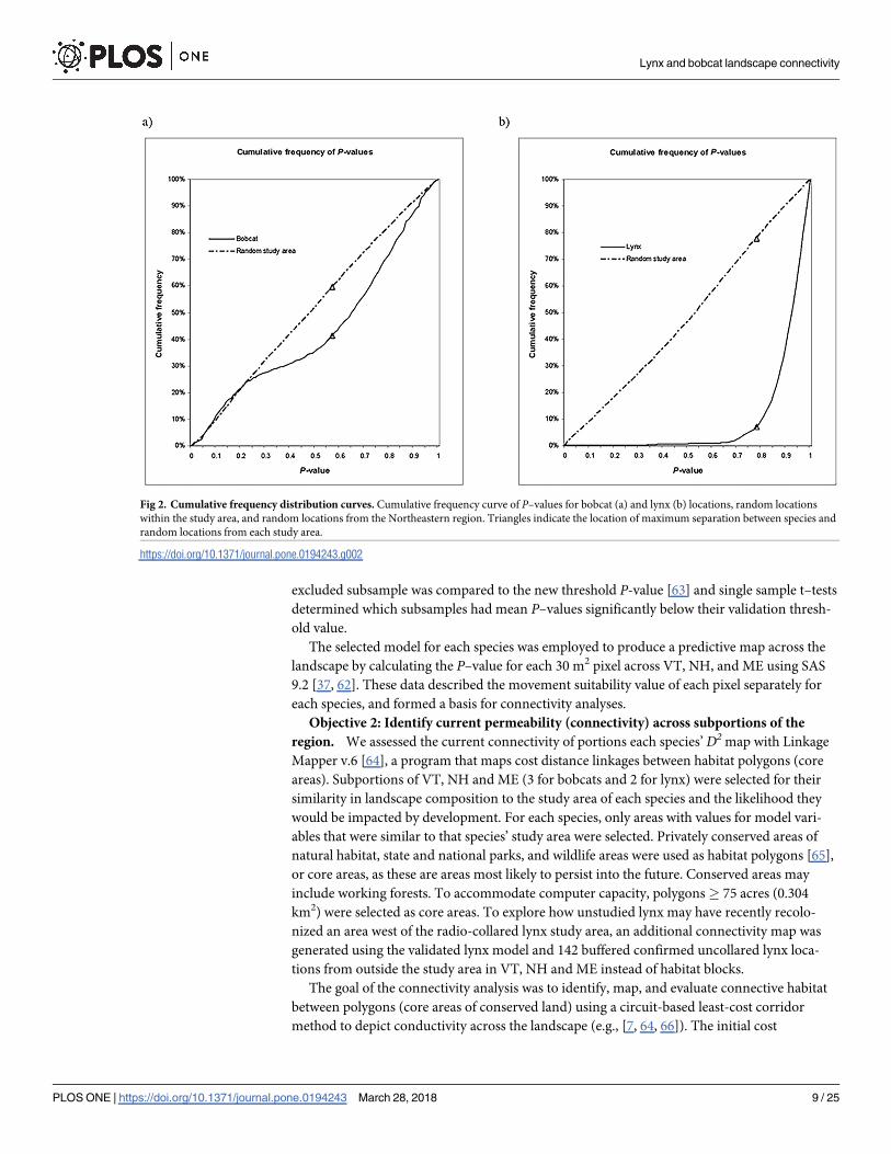
Fig 2. Cumulative frequency distribution curves. Cumulative frequency curve of P–values for bobcat (a) and lynx (b) locations, random locations

within the study area, and random locations from the Northeastern region. Triangles indicate the location of maximum separation between species and

random locations from each study area.






(resistance) of each pixel was computed as 1—P from the D2 analysis. The Linkage Mapper

tool (now integrated into Circuitscape), used the resistance map to compute multiple pathways

between each polygon (core areas of conserved habitat) and others, and then mosaicked the

results into a single composite map. The resulting map of each focal area provided an additive

estimate of the relative accessibility of each cell to the nearest core area [7, 64].

We then defined “connective habitat” for each species by overlaying GPS points on the

Linkage Mapper connectivity map and identifying the highest cost distance value used by each

species. This maximum, rounded up by 1%, was used to set a connective habitat threshold for

each species. Cost-distance pixels below this threshold were identified as “connective habitat”,

while pixels exceeding this value were deemed “non-connective habitat”.

Objective 3: Estimate the persistence of connectivity into the future in areas most likely

to experience increased anthropogenic pressure and estimate change in availability of con-

nective habitat in these areas. The projected change in the human footprint in the Northeast

[30, 67] (see also [68, 69]) was used to evaluate the impact of future development on connectiv-

ity over the next 30 years. The first human footprint analysis illustrated the relative human

influence in every biome on the land’s surface [69], utilizing 9 datasets to provide a measure of

human influence for each landscape based on factors such as human population density, land

transformation, accessibility, and electrical power infrastructure. Forecasts of the human foot-

print map for the Northeast U.S. were conducted by Trombulak et al. [30], who estimated the

human footprint over an approximate 30 year horizon at a 90m2 pixel resolution based on pro-

jected human settlement, road, and amenities over a 20 year horizon.

To determine decline in “connective habitat”, cost pixels overlapping with a projected

increase in human footprint were updated by multiplying the current cost value of each pixel

from the Linkage Mapper times the increase in human influence in that pixel. For example,

cost pixels that occurred in locations where footprint score was projected to increase by 10%

were multiplied by 1.1 to yield a projected cost. In contrast, cost pixels that occurred in loca-

tions where footprint scores were projected to decrease were adjusted downward for future

projections. For example, cost pixels that occurred in locations where footprint scores were

projected to decrease by 10% were divided by 1–0.1 = 0.9 to reflect increased connectivity in

these areas.

The projected change in “connective habitat” from the species’ perspective in the future

(the impact of projected development on connectivity) was also calculated. Each cost-distance

pixel in the future map was dichotomized as being connected or not based on the threshold

identified in Objective 2. We compared the change in connective habitat between the current

and projected landscape for each species.

Results

A total of 2,427 independent radio–collar GPS locations from 16 bobcats (5 F, 11 M) and 3,639

GPS collar locations from 31 adult lynx (10 F, 21 M) were used in these analyses [70]. Two

young adult bobcats (B11 and B44) contributed 135 locations (S2 Table); the remaining loca-

tions were from adults. The majority (89%) of bobcat locations occurred between January and

August due to collar deployment schedules [70] (S2 Fig). Lynx locations were slightly biased

towards spring months, but distributed more evenly through the year [70] (S3 Fig).

Objective 1: PCA model selection and validation and mapping of

movement suitability for each pixel

Sixty eight PCA models consisting of combinations of 31 variables were considered for bobcats

(Table 2). The greatest separation between cumulative frequencies for bobcat locations and




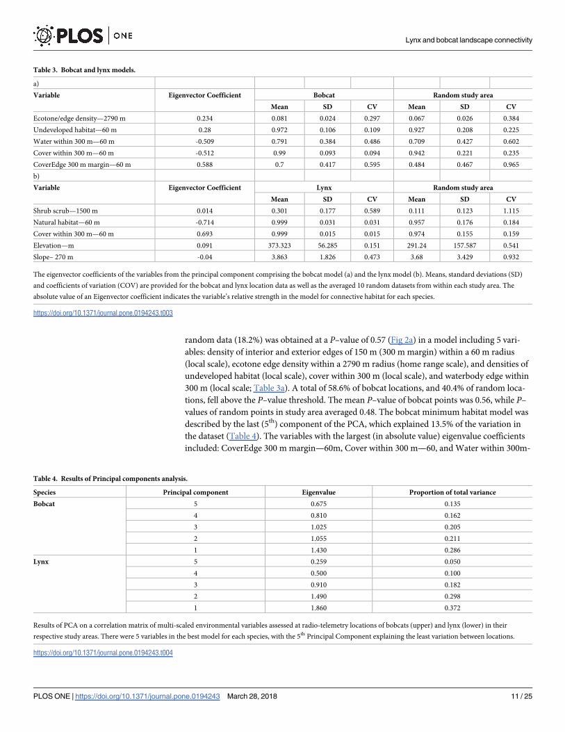
random data (18.2%) was obtained at a P–value of 0.57 (Fig 2a) in a model including 5 vari-

ables: density of interior and exterior edges of 150 m (300 m margin) within a 60 m radius

(local scale), ecotone edge density within a 2790 m radius (home range scale), and densities of

undeveloped habitat (local scale), cover within 300 m (local scale), and waterbody edge within

300 m (local scale; Table 3a). A total of 58.6% of bobcat locations, and 40.4% of random loca-

tions, fell above the P–value threshold. The mean P–value of bobcat points was 0.56, while P–

values of random points in study area averaged 0.48. The bobcat minimum habitat model was

described by the last (5th) component of the PCA, which explained 13.5% of the variation in

the dataset (Table 4). The variables with the largest (in absolute value) eigenvalue coefficients

included: CoverEdge 300 m margin—60m, Cover within 300 m—60, and Water within 300m-

Table 3. Bobcat and lynx models.

a)

Variable Eigenvector Coefficient Bobcat Random study area

Mean SD CV Mean SD CV

Ecotone/edge density—2790 m 0.234 0.081 0.024 0.297 0.067 0.026 0.384

Undeveloped habitat—60 m 0.28 0.972 0.106 0.109 0.927 0.208 0.225

Water within 300 m—60 m -0.509 0.791 0.384 0.486 0.709 0.427 0.602

Cover within 300 m—60 m -0.512 0.99 0.093 0.094 0.942 0.221 0.235

CoverEdge 300 m margin—60 m 0.588 0.7 0.417 0.595 0.484 0.467 0.965

b)

Variable Eigenvector Coefficient Lynx Random study area

Mean SD CV Mean SD CV

Shrub scrub—1500 m 0.014 0.301 0.177 0.589 0.111 0.123 1.115

Natural habitat—60 m -0.714 0.999 0.031 0.031 0.957 0.176 0.184

Cover within 300 m—60 m 0.693 0.999 0.015 0.015 0.974 0.155 0.159

Elevation—m 0.091 373.323 56.285 0.151 291.24 157.587 0.541

Slope– 270 m -0.04 3.863 1.826 0.473 3.68 3.429 0.932

The eigenvector coefficients of the variables from the principal component comprising the bobcat model (a) and the lynx model (b). Means, standard deviations (SD)

and coefficients of variation (COV) are provided for the bobcat and lynx location data as well as the averaged 10 random datasets from within each study area. The

absolute value of an Eigenvector coefficient indicates the variable’s relative strength in the model for connective habitat for each species.


Table 4. Results of Principal components analysis.

Species Principal component Eigenvalue Proportion of total variance

Bobcat 5 0.675 0.135

4 0.810 0.162

3 1.025 0.205

2 1.055 0.211

1 1.430 0.286

Lynx 5 0.259 0.050

4 0.500 0.100

3 0.910 0.182

2 1.490 0.298

1 1.860 0.372

Results of PCA on a correlation matrix of multi-scaled environmental variables assessed at radio-telemetry locations of bobcats (upper) and lynx (lower) in their

respective study areas. There were 5 variables in the best model for each species, with the 5th Principal Component explaining the least variation between locations.







60m were the stronger identifiers of pixels with high bobcat movement capability within the

model, which also included Undeveloped habitat within 60 m, and Edge density at the land-

scape scale (Table 3a).

Cross validation revealed that the bobcat model (Table 3a) adequately described 86% of the

validation sets, representing 14 of the 16 cats. The mean difference in P–values for individual

bobcats between the final model and the validation models was 0.06, suggesting that outliers

had little effect on the final model. Two male bobcats had average P–values significantly lower

than their validation model thresholds (B27 P = 0.52, threshold P = 0.61, p< 0.0001; B29

P = 0.51, threshold P = 0.57, p = 0.0024).

Eighty four PCA models consisting of combinations of 35 variables were considered for

lynx (Table 2). The lynx model showed more specialization of lynx for particular habitat:

92.91% of lynx locations, but only 22.11% of random study area locations, occurred above the

P = 0.78 threshold (Fig 2b). The mean P–value for lynx locations was 0.90, whereas random

points in the study area had an average P–value of 0.52. A maximum of 70.8% separation

between the cumulative frequencies of P–values for lynx data and random locations was found

at P = 0.78 (Fig 2b), in a model with 5 variables: availability of Shrub scrub within a 1500 m

radius (daily distance moved), Natural habitat (local scale), availability of Cover within 300 m

(local scale), Elevation, and Slope within a 270 m radius (Table 3b). Lynx habitat use was

described by the last (5th) component, which explained 4.95% of variation in the data

(Table 4). The variables with the largest (in absolute value) eigenvector coefficients were Cover

within 300m at the local scale, and Natural habitat at the local scale, and thus are key indicators

of areas with high lynx movement capability (Table 3b).

Cross validation revealed that the lynx model (Table 3b) adequately described 84% of the 19

validation sets for the 31 cats. The mean difference in P–values for validation sets between the

final model and the validation models was 0.08. Two adult males (L114 and L18) and a valida-

tion set of 3 females (L131, L141, L150) had average P–values significantly lower than valida-

tion thresholds (L114 P = 0.53, threshold P = 0.86, p< 0.00001; L18 P = 0.65, threshold

P = 0.78, p< 0.0001; L131/141/150 P = 0.64, threshold P = 0.81, p< 0.0001).

Objective 2: Map current connectivity across subportions of the region, and

then evaluate current connectivity within these subportions

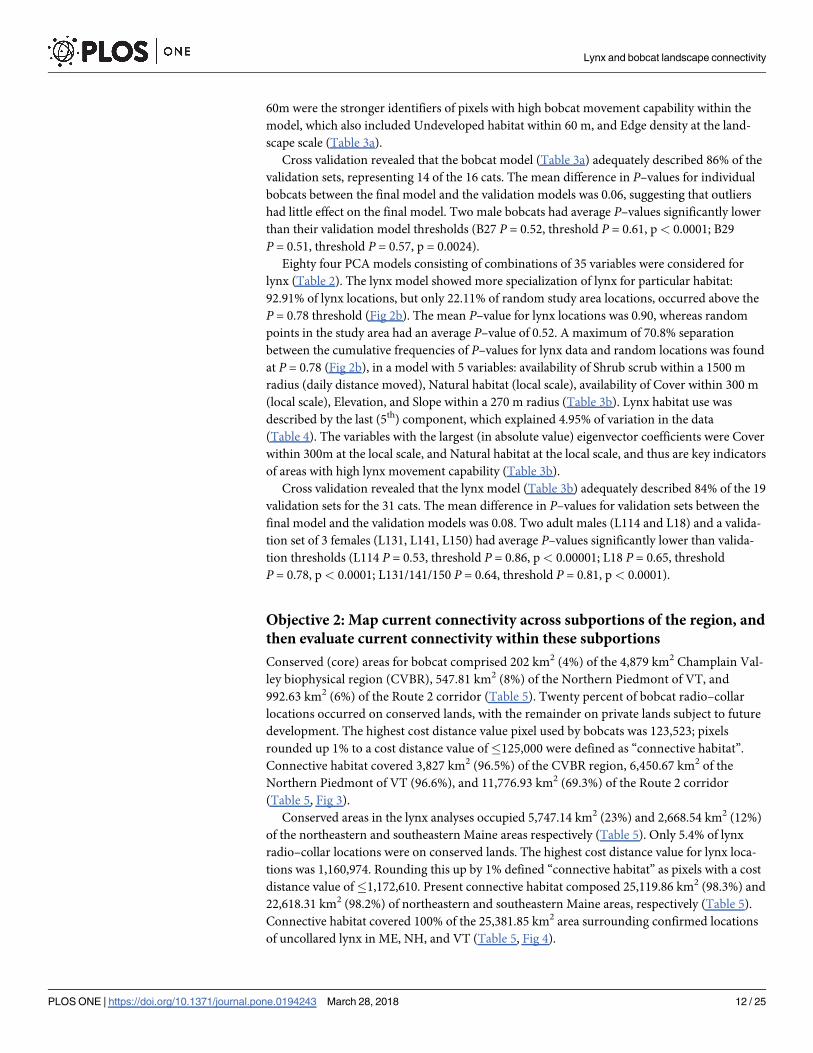
Conserved (core) areas for bobcat comprised 202 km2 (4%) of the 4,879 km2 Champlain Val-

ley biophysical region (CVBR), 547.81 km2 (8%) of the Northern Piedmont of VT, and

992.63 km2 (6%) of the Route 2 corridor (Table 5). Twenty percent of bobcat radio–collar

locations occurred on conserved lands, with the remainder on private lands subject to future

development. The highest cost distance value pixel used by bobcats was 123,523; pixels

rounded up 1% to a cost distance value of�125,000 were defined as “connective habitat”.

Connective habitat covered 3,827 km2 (96.5%) of the CVBR region, 6,450.67 km2 of the

Northern Piedmont of VT (96.6%), and 11,776.93 km2 (69.3%) of the Route 2 corridor

(Table 5, Fig 3).

Conserved areas in the lynx analyses occupied 5,747.14 km2 (23%) and 2,668.54 km2 (12%)

of the northeastern and southeastern Maine areas respectively (Table 5). Only 5.4% of lynx

radio–collar locations were on conserved lands. The highest cost distance value for lynx loca-

tions was 1,160,974. Rounding this up by 1% defined “connective habitat” as pixels with a cost

distance value of�1,172,610. Present connective habitat composed 25,119.86 km2 (98.3%) and

22,618.31 km2 (98.2%) of northeastern and southeastern Maine areas, respectively (Table 5).

Connective habitat covered 100% of the 25,381.85 km2 area surrounding confirmed locations

of uncollared lynx in ME, NH, and VT (Table 5, Fig 4).




Objective 3: Estimate the persistence of connectivity into the future in areas

most likely to experience increased anthropogenic pressure

Using projections of current growth trends to approximately 2040 [30, 58], connective habitat

for bobcats was estimated to decrease by 1,259.36 km2, (16.9%) in the CVBR, by 796.72 km2

(11.9%) across the Northern Piedmont area, and by 1,139.57 km2 (6.7%) across the Route 2

corridor (Table 5, ~ 2040 values).

Connective habitat for lynx is predicted to decrease across southeastern Maine by 784.78

km2 (3.4%) over the next 30 years, and across the area of uncollared lynx locations (west of the

Musquacook lakes study area to Vermont) by 81.35 km2 (0.3%), though connective habitat

was predicted to increase by 197.79 km2, or 0.7%, in northeastern Maine (Table 5).

Discussion

A description of habitat use should reflect how an animal experiences its environment,

which can be challenging because some species perceive habitat variables in ways that are diffi-

cult to determine [71, 72]. Other modeling methods require that variables be selected by the

researcher. Our methodology allowed selection of model variables from a wide range of land-

scape variables at different scales to determine which best predicted occurrence of a species in

an area [29, 73], based on the consistency of the variables within the data [37, 59].

Our results support previous findings that bobcats utilize a wide variety of resources [74],

whereas lynx are more specific in their habitat use [75]. The separation of P–value cumulative

frequency curves between species and random study area data illustrated that bobcats used a

Table 5. Conserved core areas and connective habitat.

a)

Bobcat area location Area (km2) Time Conserved Areas (km2) % Connective habitat

Area (km2) %

Champlain Valley biophysical region 3964.9 Present 202.31 5 3827.21 96.5

3226.7� ~2040 156.51� 5 2567.85 79.6

Northern Piedmont area of VT 6677.3 Present 547.81 8 6450.67 96.6

- ~2040 - - 5653.95 84.7

Route 2, VT through Augusta ME 16996.8 Present 992.63 6 11776.93 69.3

- ~2040 - - 10637.36 62.6

b)

Lynx area location Area (km2) Time Conserved Areas (km2) % Connective habitat

Area (km2) %

Northeast Maine 25566.90 Present 5747.14 23 25119.86 98.3

- ~2040 25317.65 99

Southeast Maine 23028.73 Present 2668.54 12 22618.31 98.2

- ~2040 21833.53 94.8

Confirmed locations—VT, NH, ME 25381.85 Present 37.4�� 25380.46�� 100

- ~2040 25299.11 99.7

Extent of conserved core areas and connective habitat within each of the areas evaluated for bobcat (a) and lynx (b), and the impact of development projected to the year

2040. Connective habitat areas, which include core habitat, are defined by the highest cost distance pixel used by each species. For bobcats this value is 123,523 (rounded

to 125,000); for lynx it is 1,160,974 (1,172,610).

�As the future human footprint is not calculated for the entire Champlain Valley, the future area is smaller.

��Recent (1999–2011) buffered confirmed locations of uncollared lynx in VT, NH, and ME are used instead of conserved areas.

��The area difference of uncollared locations and present connective habitat is due to rounding error between raster and polygon layers.






wider range of habitat values (available habitat) than lynx (Fig 2), as their location data had less

departure from random location data (Fig 2a) than the lynx data (Fig 2b). Variables included

in the final model indicated that bobcat presence is more influenced by general landscape

structure and characteristics including availability of edge, cover, and riparian and undevel-

oped habitats than specific habitat types, which is consistent with other studies [76–78]. That

two different measures and scales of edge—ecotone density at the home range scale, and

Fig 3. Present and predicted connectivity for bobcats. Present (a) and predicted future (b) connectivity for bobcats

between conserved areas of natural habitat in the Champlain Valley Biophysical Region (upper left), the Northern

Piedmont area of Vermont (upper right) and below, along the Route 2 corridor from Vermont into southern Maine

(bottom). The core polygons have a cost distance of 0, and are the basis of the orange areas in the maps. Connective

habitat for bobcats is defined as pixels with a cost distance value� 125,000 (small arrow on legend). Future

connectivity between conserved areas was predicted only where anthropogenic change has been estimated by

Trombulak et al. [30].






density of edge at a local scale—were elements of the final model suggests that this landscape

characteristic is important to bobcats. Indeed, the bobcat’s range has expanded northward as

forests were fragmented, increasing edge [79, 80]. Bobcats were also found to select for edges

and against interior forests at finer scales in the Champlain Valley [81], presumably in

response to the combination of prey density and availability of dense cover for movement and

stalking prey [82, 83]. Bobcat home range size in Mississippi was predicted by edge density;

patches of cover with a large perimeter:interior ratio that provide more edge may lower search

times for prey venturing outside the patch edge [78]. Lower cross validation scores for males of

both species may indicate they are more likely to use suboptimal habitat in moving over wider

areas, partly to access multiple female ranges [54, 84]. The two bobcats with lower validation

scores were adults; further knowledge of their exact age, health and breeding status, as well as

surrounding landscape changes, would have been informative.

In contrast to bobcats, which used undeveloped habitat including agricultural lands, lynx

were closely associated only with natural habitats. Natural habitat and proximity to cover were

essentially consistent among locations (Table 3). Lynx reliance on larger scale variables

supports Fuller and Harrison [85], who found lynx select large patches of habitat with high

prey density rather than areas within patches. Low use of areas with P–values < 0.8 (Fig 2b)

suggests that this species is highly selective. Inclusion of elevation in the model supports a

strong association of lynx with deeper snow found in other studies [86]. The boundary

between bobcat and lynx ranges is often defined by deeper snow, where lynx might also be

Fig 4. Present and predicted connectivity for lynx. Present (a) and predicted future (b) connectivity for lynx between conserved areas of natural

habitat in northeastern and southeastern Maine (left and middle, respectively), and between confirmed uncollared lynx locations from ME, NH, and

VT (right). The core polygons have a cost distance of 0, and are the basis of the orange areas in the maps. Connective habitat for lynx is defined as pixels

with a cost distance value�1,172,610 (small arrow on legend). Future connectivity between conserved areas was predicted only where anthropogenic

change has been estimated by Trombulak et al. [30].






able to escape competition from coyotes (Canis latrans) [83, 87]. Climate change may reduce

snow depth in the future, contracting the lynx range [88] and expanding the bobcat range.

Connectivity

Anthropogenic development is expected to have different impacts on connectivity for lynx

and bobcats in the areas we studied. Mapping connective areas using circuit-based least-cost

path analysis and examining how anthropogenic changes are likely to impact the landscape at

a 30 m x 30 m resolution identified areas of this multiuse landscape where connectivity could

decline substantially (Figs 3 and 4, Table 5). In the absence of suitable new protected areas,

connective habitat for bobcats is predicted to decline in all areas studied, and movements

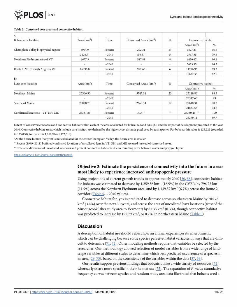
between subpopulations of bobcats may decrease. For example, connectivity is currently

largely intact across much of the eastern portion of Route 2 around Auburn and Lewiston,

Maine (Fig 5). Although the Route 2 corridor as a whole is predicted to experience the smallest

overall decline in connective habitat for bobcats of the three areas examined (Table 5),

subportions predicted to undergo decline were concentrated, and these areas will experience

restricted connectivity (Figs 5 and 3). Strategic planning and conservation of additional lands

in areas expected to experience increased anthropogenic activity could minimize the impacts

of development on future landscape connectivity for bobcats.

In contrast to bobcats, lynx connectivity is expected to remain stable in most areas exam-

ined. Connective habitat in southeastern Maine is predicted to undergo contraction in some

areas and localized expansion in others (Fig 4), such that the impact of the increased human

footprint in localized areas is not apparent when looking at numerical estimates of decline in

area of connective habitat (Table 5). Although concentrated development could affect the

future dispersal ability of lynx to southeast Maine, suitable habitat could also diminish with a

warming climate [88]. Declines in connective habitat are expected to be minimal in areas

between confirmed locations of uncollared lynx and do not appear to obstruct overall dispersal

ability (Table 5; Fig 4 right), allowing continued recolonization of lynx across this portion of

their former range with favorable snowdepth. Overall, connectivity is not expected to decline

for lynx across their breeding range in northern New England; and an increase in connective

habitat in northeastern Maine (Table 5, Fig 4) may even assist long-distance movement of ani-

mals between breeding populations in Canada and the US.

Scope and limitations of the method

Our approach provides a conservative illustration of future connectivity, especially for bobcats,

because: 1) models for each species are based on data largely from adults, who are less likely to

disperse, so connectivity mapping is conservative. Only two of the animals, bobcats B11 and

B44, were subadults and these cats have relatively few data points (33 and 102 respectively).

Thus, the models largely reflect habitat use of individuals settled into home ranges; 2) bobcats

are flexible in their habitat use, which allows them to occupy such a wide variety of habitats

lower 48 United States and Mexico [71, 80]. Because our models reflect habitats found in the

Northeastern US, they are best applied to this region; and 3) we used permanently conserved

areas as habitat blocks, and assumed that conserved areas of natural habitat are suitable for

each species. The loss of connectivity is not calibrated to the increase in human footprint pro-

jections of Trombulak et al. [30], so the time line of these predictions may vary from theirs,

and periodic reevaluation is recommended.

Several caveats in terms of modeling species’ distribution are worth highlighting. First,

depending on species, analysis by sex and age, and analyses of habitat use by season and time

of day could be informative if the data were robust enough. Information on temporal use of




Fig 5. Subportion of area where connectivity is expected to decline. The impact of future development on

connective habitat for bobcats in a portion of southeastern Maine around Auburn and Lewiston. Black describes areas

of connective habitat, white defines pixels with a cost distance value greater than 125,000, above the maximum cost

distance value used by bobcats.






habitats by species could allow schedule adjustments of landscape use by humans to also allow

wildlife use. Second, although there is evidence that snow depth affects distribution of lynx

and bobcats, it was not possible to correlate locations with snowdepth due to the lack of local-

ized detail in the snowdepth data that were available. Elevation was suggested to provide some

proxy for this. Third, it should be noted that connectivity is not always a gain for populations;

depending on configuration, it can also facilitate the spread of emerging diseases and invasive

species [89, 90].

Only areas with variable values similar to those of the study areas for each species were

selected for connectivity modeling, as we assumed the models applied best to these landscapes.

Though there is cohesion of individuals to the models (S4 Fig), there are subpixel landscape

features, including narrow hedgerows that animals use, which are not discernable in a 30

meter pixel. Although there is no detailed confirmation of either model by dispersing animals

after the data were taken, less than a year after the conclusion of the modeling and mapping,

lynx were confirmed to be breeding in northeastern Vermont, in an area predicted as most

favorable habitat by the 30 meter pixel suitability model.

Conclusion

A sufficient network of connective habitat can facilitate evolutionary responses to climate

change in a fragmented landscape by allowing species to adjust ranges [91, 92]. Predictions of

future connectivity rely on how much of the resulting matrix of core and connective habitat

persists through time. Much of the habitat in the Northeast is under private ownership, and

not conserved. If additional areas are conserved, especially in pinch points identified in smaller

scale views of the 30 m2 pixel maps (i.e. Fig 5; also see [93]), prospects for future connectivity

could improve. Regular monitoring and evaluation of anthropogenic and climate induced

changes on connectivity will be necessary for unbiased mapping. By considering the influence

of future landscape changes [94], and adapting management as science is updated [95, 96], we

can plan for and adaptively manage range adjustment by both plant and animal species [89,

97–102].

Information on the ability of wide–ranging species to negotiate a human–modified land-

scape can inform efforts to construct and manage functional connectivity for wildlife, help-

ing to plan a landscape that accommodates both humans and wildlife. Behavioral studies of

how focal species negotiate these landscapes spatially and temporally are integral to any

models. Investigations of landscape use should be conducted at scales that are realistic to the

species studied, even when connectivity is to be projected across large areas [22]. A land-

scape accommodating bobcat movement would include sufficient edge and undeveloped

habitats. As bobcats appear to cue into landscape features at a smaller local scale, smaller

portions of essential elements in a heterogeneous landscape would suffice to encourage bob-

cat movement between areas of core habitat. Both bobcats and lynx require access to cover.

Larger areas of coniferous natural habitat, interspersed with areas of regenerating coniferous

sapling or shrub scrub supporting sufficient prey, would provide connectivity for lynx [20,

70].

It is important to emphasize that habitat maps do not predict presence of a species, but

rather illustrate areas a species may be able to access. Interactions with other species, human

activity, human use of adjacent areas, and other variables not explored in our analyses can

affect distribution. The majority of lynx and bobcat locations used were on private lands, and

these areas can be subject to rapid change. Confirmed presence of breeding animals in an area

from field surveys can help prioritize areas for conservation [103, 104]. We suggest that pres-

ence of target species, distribution of undeveloped areas, effects of climate change, human use




of areas, and predicted development be reassessed periodically to guide efforts to maintain

regional connectivity for bobcats, lynx and other wide–ranging species.

Supporting information

S1 Methods. Map layers. Construction of 108 map layers, each a variable considered in mod-

els. This supplement describes the maps in Table 1, and their construction.

(DOC)

S2 Methods. Analysis overview.

(DOCX)

S1 Table. Bobcat location data used for analyses.

(XLS)

S2 Table. Capture data, and information on dates and numbers of locations used per bob-

cat. Data for four bobcats with large datasets was selected to even out distribution of data

through the year. A star� in the Used location dates column indicates that locations from these

cats were selected for months that were lacking elsewhere in the dataset. A~ for B4 and B11

indicates that these were young adults at the time data were gathered, and possibly dispersing.

(TIF)

S3 Table. Capture data, and information on dates and numbers of locations used per lynx

collar. Six lynx were recaptured and recollared and data from multiple collars used (i.e. L140

has 35+11 locations). Data was taken from the full range of dates for all lynx. All lynx providing

data were adults.

(TIF)

S1 Fig. Bobcat habitat P–values mapped by 30 m2 pixel across Vermont, New Hampshire

and Maine, with bobcat study area indicated.

(TIF)

S2 Fig. Months of bobcat locations used in modeling, by cat. Dashed lines indicate that not

all locations from that month were used, and that locations were selected to even out locations

over the year.

(TIF)

S3 Fig. Months of lynx locations used in modeling, by cat.

(TIF)

S4 Fig. Close up of bobcat connectivity map, with bobcat locations layered on top.

(TIF)

Acknowledgments

We thank Walter Jakubas, of Maine Department of Inland Fisheries and Wildlife, for gener-

ously allowing the use of the lynx data in these analyses. The Vermont Advanced Computing

Center and The Rubenstein School at University of Vermont provided computers. We thank

Jennifer Morrow; Bob Devins; Christopher Hoving; Guoping Tang; T. Garin (Advanced

Telemetry Systems); Tony Tur and Rachel Cliche of US Fish and Wildlife; Chris Bernier; wild-

life agencies in Maine, New Hampshire and Vermont; and Joe Roman, for logistical support,

assistance, and data sharing. Use of trade names or products does not constitute endorsement

by the U.S. Government. The Vermont Cooperative Fish and Wildlife Research Unit is jointly



http://www.plosone.org/article/fetchSingleRepresentation.action?uri=info:doi/10.1371/journal.pone.0194243.s001










supported by the U.S. Geological Survey, University of Vermont, Vermont Department of

Fish and Wildlife, and Wildlife Management Institute.

Author Contributions

Conceptualization: Laura E. Farrell, Daniel M. Levy, Therese Donovan, Ruth Mickey, Alan

Howard.

Data curation: Laura E. Farrell, Daniel M. Levy, Therese Donovan, Alan Howard, Jennifer

Vashon, Mark Freeman.

Formal analysis: Laura E. Farrell, Daniel M. Levy, Therese Donovan, Ruth Mickey, Alan

Howard.

Funding acquisition: Laura E. Farrell, Therese Donovan, Kim Royar.

Investigation: Laura E. Farrell, Therese Donovan, Jennifer Vashon, Mark Freeman, Kim

Royar.

Methodology: Laura E. Farrell, Daniel M. Levy, Therese Donovan, Ruth Mickey, Alan

Howard.

Project administration: Laura E. Farrell, Therese Donovan, C. William Kilpatrick.

Resources: Laura E. Farrell, Therese Donovan, Jennifer Vashon, Kim Royar, C. William

Kilpatrick.

Software: Laura E. Farrell, Daniel M. Levy, Alan Howard.

Supervision: Laura E. Farrell, Therese Donovan, C. William Kilpatrick.

Validation: Laura E. Farrell, Ruth Mickey, Alan Howard.

Visualization: Laura E. Farrell, Daniel M. Levy, Ruth Mickey, Alan Howard.

Writing – original draft: Laura E. Farrell, Therese Donovan, C. William Kilpatrick.

Writing – review & editing: Laura E. Farrell, Therese Donovan, Ruth Mickey, Jennifer

Vashon.

References1. Vashon J, McLellan S, Crowley S, Meehan A, Laustsen K. Canada lynx assessment. 2012. Maine

Department of Inland Fisheries and Wildlife. 107 p. http://www.maine.gov/ifw/docs/species_planning/

mammals/canadalynx/Lynx%20Assessment%202012_Final.pdf

2. New Hampshire Fish and Game. Canada lynx documented in northern New Hampshire. 2011. http://

www.wildlife.state.nh.us/Newsroom/News_2011/news_2011_Q4/lynx_documented_120911.html.

Accessed 23 December 2011.

3. Linforth J, Cliche R. Canada Lynx Coming Back to Vermont. 2013. http://www.fws.gov/endangered/

map/ESA_success_stories/VT/VT_story2/. Accessed 14 Feb 2014.

4. Woolmer G, Trombulak SC, Ray JC, Doran PJ, Anderson MG, Baldwin RF, et al. Rescaling the

human footprint: A tool for conservation planning at an ecoregional scale. Landsc and Urban Plan

2008; 87: 42–53.

5. Foster D, Donahue B, Kittredge D, Lambert F, Hunter M, Hall BR, et al. Wildlands and Woodlands—A

Vision for the New England Landscape. Harvard Forest, Harvard University. Petersham, MA. 2010.

36 p.

6. Swingland IR, Greenwood PJ. The ecology of animal movement. New York: Oxford University Pres;

1984.

7. Singleton PH, Gaines WL, Lehmkuhl JF. Landscape permeability for large carnivores in Washington:

a geographic information system weighted–distance and least–cost corridor assessment. Research



http://www.maine.gov/ifw/docs/species_planning/mammals/canadalynx/Lynx%20Assessment%202012_Final.pdf

http://www.maine.gov/ifw/docs/species_planning/mammals/canadalynx/Lynx%20Assessment%202012_Final.pdf

http://www.wildlife.state.nh.us/Newsroom/News_2011/news_2011_Q4/lynx_documented_120911.html

http://www.wildlife.state.nh.us/Newsroom/News_2011/news_2011_Q4/lynx_documented_120911.html

http://www.fws.gov/endangered/map/ESA_success_stories/VT/VT_story2/

http://www.fws.gov/endangered/map/ESA_success_stories/VT/VT_story2/


Paper PNW–RP–549. Portland, OR: U.S. Department of Agriculture, Forest Service, Pacific North-

west Research Station; 2002. 89 p.

8. Hanski IL, Gilpin ME. Metapopulation biology: ecology, genetics, and evolution. San Diego: Academic

Press. 512 p. 1997.

9. Hale ML, Lurz PW, Shirley MD, Rushton S, Fuller RM, Wolff K. Impact of landscape management on

the genetic structure of red squirrel populations. Science 2001; 293: 2246–2248. https://doi.org/10.

1126/science.1062574 PMID: 11567136

10. Knick ST, Bailey TN. Long distance movements by two bobcats from southeastern Idaho. Am Midl Nat

1986; 116: 221–223.

11. Slough BG, Mowat G. Lynx population dynamics in an untrapped refugium. J Wildl Manag 1996; 60:

946–961.

12. Crooks K. Relative sensitivities of mammalian carnivores to habitat fragmentation. Conserv Biol 2002;

16: 488–502.

13. Riley SPD, Sauvajot RM, Fuller TK, York EC, Kamradt DA, Bromley C, et al. Effects of urbanization

and habitat fragmentation on bobcats and coyotes in southern California. Conserv Biol 2003; 17: 566–

576.

14. Hilty JA, Merenlender AM. Use of riparian corridors and vineyards by mammalian predators in northern

California. Conserv Biol 2004; 18: 126–135.

15. Lovallo MJ, Anderson EM. Bobcat (Lynx rufus) home range size and habitat use in northwest Wiscon-

sin. Am Midl Nat 1996; 135: 241–252.

16. Tigas L, Van Vuren DH, Sauvajot RM. Behavioral responses of bobcats and coyotes to habitat frag-

mentation and corridors in an urban environment. Biol Conserv 2002; 108: 299–306.

17. Roland J, Taylor PD. Insect parasitoid species respond to forest structure at different spatial scales.

Nature 1997; 386: 710–713.

18. MacFaden SW, Capen DE. Avian habitat relationships at multiple scales in a New England forest. For-

est Science 2002; 48: 243–253.

19. Chamberlain MJ, Leopold BD, Conner LM. Space use, movements and habitat selection of adult bob-

cats (Lynx rufus) in central Mississippi. Am Midl Nat 2003; 149: 395–405.

20. Vashon JH, Meehan AL, Organ JF, Jakubas WJ, McLaughlin CR, Vashon AD, et al. Diurnal habitat

relationships of Canada lynx in an intensively managed private forest landscape in northern Maine. J

Wildlife Manage 2008a; 72: 1488–1496.

21. Basille M, Van Moorter B, Herfindal I, Martin J, Linnell JDC, Odden J, et al. Selecting Habitat to Sur-

vive: The Impact of Road Density on Survival in a Large Carnivore. PLoS ONE 2013; 8(7): https://doi.

org/10.1371/journal.pone.0065493

22. Ohmark SM, Iason GR, Palo RT. Spatially segregated foraging patterns of moose (Alces alces) and

mountain hare (Lepus timidus) in a subarctic landscape: different tables in the same restaurant? Cana-

dian Journal of Zoology. 2015; 93(5):391–6.

23. Lindenmayer DB. Factors at multiple scales affecting distribution patterns and its implications for ani-

mal conservation—Leadbeater’s Possum as a case study. Biodiv Conserv 2000; 9: 15–35.

24. Cushman SA, Landguth EL. Scale dependent inference in landscape genetics. Landsc Ecol 2010; 25:

967–979.

25. Lyra–Jorge MC, Ribeiro MC, Ciocheti G, Tambosi LR, Pivello VR. Influence of multi–scale landscape

structure on the occurrence of carnivorous mammals in a human–modified savanna, Brazil. Europ J

Wildl Research 2010; 56: 359–368.

26. Thompson CM, McGarigal K. The influence of research scale on bald eagle habitat selection along the

lower Hudson River, New York. Landscape Ecol 2002; 17: 569–586.

27. Cushman SA, McKelvey KS, Schwartz MK. Use of empirically derived source–destination models to

map regional conservation corridors. Conserv Biol 2009; 23: 368–376. https://doi.org/10.1111/j.1523-

1739.2008.01111.x PMID: 19016821

28. Mayor SJ, Schneider DC, Schaefer JA, Mahoney SP. Habitat selection at multiple scales. Ecoscience

2009; 16: 238–247.

29. Thornton DH, Branch LC, Sunquist ME. The influence of landscape, patch, and within–patch factors

on species presence and abundance: a review of focal patch studies. Landscape Ecol 2011; 26: 7–18.

30. Trombulak S, Anderson M, Baldwin R, Beazley K, Ray J, Reining C. The Northern Appalachian/Aca-

dian ecoregion: Priority locations for conservation action. Two Countries, One Forest Special Report

No.1; 2008. 58 p. http://www.2c1forest.org/en/resources/resources.html. Accessed 9 October 2013.



https://doi.org/10.1126/science.1062574


http://www.ncbi.nlm.nih.gov/pubmed/11567136



https://doi.org/10.1111/j.1523-1739.2008.01111.x

https://doi.org/10.1111/j.1523-1739.2008.01111.x


http://www.2c1forest.org/en/resources/resources.html


31. Abrahms B, Sawyer SC, Jordan NR, Weldon McNutt J, Wilson AM, Brashares JS, et al. Does wildlife

resource selection accurately inform corridor conservation? J Appl Ecol 2017; 54:412–422 https://doi.

org/10.1111/1365-2664.12714

32. Walpole AA, Bowman J, Murray DL, Wilson PJ. Functional connectivity of lynx at their southern range

periphery in Ontario, Canada. Landsc Ecol 2012; 27:761–773.

33. Squires JR, DeCesare NJ, Olson LE, Kolbe JA, Hebblewhite M, Parks SA. Combining resource selec-

tion and movement behavior to predict corridors for Canada lynx at their southern range periphery.

Biolog Conserv 2013; 157:187–195.

34. Reed GC, Litvaitis JA, Callahan C, Carroll RP, Litvaitis MK, Broman DJA. Modeling landscape connec-

tivity for bobcats using expert-opinion and empirically derived models: how well do they work? Anim

Conserv 2017; 20: 308–320. https://doi.org/10.1111/acv.12325

35. Zeller KA, Vickers TW, Ernest HB, Boyce WM. Multi-level, multi-scale resource selection functions

and resistance surfaces for conservation planning: Pumas as a case study. PLoS ONE 2017; 12(6):

e0179570. https://doi.org/10.1371/journal.pone.0179570. PMID: 28609466

36. Rotenberry JT, Knick ST, Dunn J. A minimalist approach to mapping species’ habitat: Pearson’s

planes of closest fit. In: Scott JM, Heglund PJ, Morrison ML, Haufler JB, Raphael MG, Wall WA, Sam-

son FB, editors. Predicting Species Occurrences: Issues of Accuracy and Scale. Island Press;

2002. pp 281–289.

37. Rotenberry JT, Preston KL, Knick ST. GIS–based niche modeling for mapping species’ habitat. Ecol-

ogy 2006; 87: 1458–1464. PMID: 16869421

38. Thompson EH, Sorenson ER. Wetland, woodland, wildland: a guide to the natural communities of Ver-

mont. Lebanon, New Hampshire: The Nature Conservancy and the Vermont Department of Fish and

Wildlife; 2005. 456 p.

39. Donovan TM, Freeman M, Abouelezz H, Royar K, Howard A, Mickey R. Quantifying home range habi-

tat requirements for bobcats (Lynx rufus) in Vermont, USA. Biological Conserv 2011; 144: 2799–2809.

40. Sorenson, E. and J. Osborne. Vermont Habitat Blocks and Habitat Connectivity: An Analysis using

Geographic Information Systems. Vermont Fish and Wildlife Department. Montpelier, VT. 2014. http://

www.vtfishandwildlife.com/UserFiles/Servers/Server_73079/File/Conserve/Vermont_Habitat_

Blocks_and_Habitat_Connectivity.pdf

41. Ballinger N. Lake Champlain Basin Program and Northern Cartographic. Population. 2004 [cited 20

December 2017]. In: People and Economy. Lake Champlain Basin Atlas, 2004 edition [Internet]. http://

atlas.lcbp.org/HTML/so_pop.htm

42. Weernetwerk. U.S. Climate Data. Clayton Lake, ME. 2017. [cited 20 December 2017]. In: https://www.

weernetwerk.nl/ [Internet]. https://usclimatedata.com/climate/clayton-lake/maine/united-states/

usme0083

43. Vashon JH, Meehan AL, Jakubas WJ, Organ JF, Vashon AD, McLaughlin CD, et al. Spatial ecology of

a Canada lynx population in Northern Maine. J Wildlife Manage 2008b; 72: 1479–1487.

44. Rettie WJ, McLoughlin PD. Overcoming radio–telemetry bias in habitat–selection studies. Can J Zool

1999; 77: 1175–1184.

45. Adams AL, Dickinson KJM, Robertson BC, van Heezik Y. An evaluation of the accuracy and perfor-

mance of lightweight GPS collars in a suburban environment. PLoS ONE 2013; 8(7): e68496. https://

doi.org/10.1371/journal.pone.0068496 PMID: 23874645

46. Parent J, Hurd J. Landscape Fragmentation Tool (LFT) v2.0. Center for Land use Education and

Research. University of Connecticut. 2009. http://clear.uconn.edu/tools/lft/lft2/. Accessed 9 June

2011.

47. Van Rossum G. Python 2.4.1. 2005. Python Software Foundation, Amsterdam, Netherlands.

48. Abouelezz HA Quantifying Bobcat (Lynx rufus) habitat and home range analysis for Northwestern and

Central Vermont. M.Sc. Thesis, University of Vermont, 2009.

49. Bailey TN. Social organization in a bobcat population. J Wildl Manage 1974; 38: 435–446.

50. Wassmer DA, Guenther DD, Layne JN. Ecology of the bobcat in south–central Florida. Bulletin of the

Florida State Museum of Biological Science 1988; 33: 159–228.

51. Ward RMP, Krebs CJ. Behavioral responses of lynx to declining snowshoe hare abundance. Can J

Zool 1985; 63: 2817–2824.

52. Kesterson MD. Lynx home range and spatial organization in relation to population density and prey

abundance. Thesis. Fairbanks: University of Alaska. 1988.

53. Squires JR, Laurion T. Lynx home range and movements in Montana and Wyoming: preliminary

results. In: Ruggiero LF, Aubry KB, Buskirk SW, Koehler GM, Krebs CJ, McKelvey KS, et al, editors.



https://doi.org/10.1111/1365-2664.12714

https://doi.org/10.1111/1365-2664.12714

https://doi.org/10.1111/acv.12325




http://www.vtfishandwildlife.com/UserFiles/Servers/Server_73079/File/Conserve/Vermont_Habitat_Blocks_and_Habitat_Connectivity.pdf



http://atlas.lcbp.org/HTML/so_pop.htm

http://atlas.lcbp.org/HTML/so_pop.htm

https://www.weernetwerk.nl/

https://www.weernetwerk.nl/

https://usclimatedata.com/climate/clayton-lake/maine/united-states/usme0083

https://usclimatedata.com/climate/clayton-lake/maine/united-states/usme0083




http://clear.uconn.edu/tools/lft/lft2/


Ecology and conservation of lynx in the United States. Niwot, CO: University Press of Colorado.

2000. pp. 337–350.

54. Eisenberg JF. Life history strategies of the Felidae: variations on a common theme. In: Miller SD, Ever-

ett DD, editors. Cats of the World: Biology, Conservation, and Management. Washington DC:

National Wildlife Federation; 1986. pp. 293–303.

55. Lariviere S, Walton LR. Lynx rufus. Mammalian Species 1997; 563: 1–8.

56. Litvaitis JA, Tash JP, Stevens CL. The rise and fall of bobcat populations in New Hampshire: Rele-

vance of historical harvests to understanding current patterns of abundance and distribution. Biol Con-

serv 2006; 128: 517–528.

57. Watrous K, Donovan TM, Mickey RM, Darling SR, Hicks AC, von Oettingen SL. Predicting minimum

habitat characteristics for the Indiana bat in the Champlain Valley. J Wildl Manag 2006; 70: 1228–

1237.

58. Clark JD, Dunn JE, Smith KG. A multivariate model of female black bear habitat use for a geographic

information system. J Wildl Manag 1993; 57: 519–526.

59. Thatcher CA, van Manen FT, Clark JD. A habitat assessment for Florida panther population expansion

into central Florida. J Mammal 2009; 90: 918–925.

60. Farber O, Kadmon R. Assessment of alternative approaches for bioclimatic modeling with special

emphasis on the Mahalanobis distance. Ecol Model 2003; 160: 115–130.

61. Friar JL, Nielsen SE, Merrill EH, Lele SR, Boyce MS, Munro RH, et al. Removing GPS collar bias in

habitat selection studies. J Appl Ecol 2004; 41: 201–212.

62. Duncan, L, Dunn JE. Partitioned Mahalanobis D2 to improve GIS classification. Paper 198–26, Pro-

ceedings SAS Users Group International No. 26. SAS Institute. 2001.

63. Verbyla DL, Litvaitis JA. Resampling methods for evaluating classification accuracy of wildlife habitat

models. Environmental Manage 1989; 13: 783–787.

64. McRae BH, Kavanagh DM. Linkage Mapper Connectivity Analysis Software. The Nature Conser-

vancy, Seattle WA. 2011. http://www.circuitscape.org/linkagemapper. Accessed September 2011.

65. Conservation Biology Institute. PADUS 1.1, Northeast Region. Protected Areas—Northeast Region.

May 2010. http://app.databasin.org/app/pages/personPage.jsp?id=consbio. Accessed Apr 15, 2011.

66. Beier P, Majka DR, Spencer WD. Forks in the road: choices in procedures for designing wildland link-

ages. Conserv Biol 2008; 22: 836–851. https://doi.org/10.1111/j.1523-1739.2008.00942.x PMID:

18544090

67. Two Countries, One Forest. The difference between the current Human Footprint and the 2040 Future

Human Footprint Current Trends Scenario. 2007. Version 1.0, raster digital data. http://www.

2c1forest.org/atlas/datawarehouse.html. Accessed 25 July 2011.

68. Sanderson EW, Jaiteh M, Levy MA, Redford KH, Wannebo AV, Woolmer G. The human footprint and

the last of the wild. BioScience 2002a; 52(10): 891–904.

69. Sanderson EW, Redford KH, Vedder A, Ward SE, Coppolillo PB. A conceptual model for conservation

planning based on landscape species requirements. Landsc Urban Planning 2002b; 58: 41–56.

70. Farrell LE. Northeastern mesomammals: landscape use and detection. Dissertation, University of Ver-

mont. 2012.

71. Sunquist ME, Sunquist FC. Ecological constraints on predation by large felids. In: Gittleman JL, editor.

Carnivore behavior, ecology and evolution. London: Chapman and Hall. 1989. pp. 283–301.

72. Wiens JA, Milne BT. Scaling of ‘landscapes’ in landscape ecology, or, landscape ecology from a bee-

tle’s perspective. Landscape Ecol 1989; 3: 87–96.

73. Bar Massada AB, Radeloff VC. Two multi–scale contextual approaches for mapping spatial pattern.

Landscape Ecol 2010; 25: 711–725.

74. Kolowski JM, Woolf A. Microhabitat use by bobcats in southern Illinois. J Wildl Manage 2002; 66: 822–

832.

75. O’Donoghue M, Boutin S, Krebs CJ, Zuleta G, Murray DL, Hofer EJ. Functional responses of coyotes

and lynx to the snowshoe hare cycle. Ecology 1998; 79: 1193–1208.

76. Kuehl AK, Clark WR. Predator activity related to landscape features in northern Iowa. J Wildl Manage

2002; 66: 1224–1234.

77. Ng SJ, Dole J, Sauvajot RM, Riley SPD, Valone T. Use of highway undercrossings by wildlife in south-

ern California. Biol Conserv 2004; 114: 499–507.

78. Constible JM, Chamberlain MJ, Leopold BD. Relationships between landscape pattern and space use

of three mammalian carnivores in central Mississippi. Am Midl Nat 2006; 155: 352–362.



http://www.circuitscape.org/linkagemapper

http://app.databasin.org/app/pages/personPage.jsp?id=consbio

https://doi.org/10.1111/j.1523-1739.2008.00942.x


http://www.2c1forest.org/atlas/datawarehouse.html

http://www.2c1forest.org/atlas/datawarehouse.html


79. Seton ET. Lives of game animals: cats, wolves, and foxes, vol. 1. Garden City, NY: Doubleday;

1925. 640 p.

80. Sunquist ME, Sunquist F. Wild cats of the world. Chicago: University of Chicago Press; 2002.

81. Cejtin M. National Land Cover Database (NLCD 2001) limitations regarding bobcat habitat assess-

ment in the Champlain Valley of Vermont. Undergraduate Thesis. 2011. University of Vermont:

Rubenstein School of Environment and Natural Resources.

82. Litvaitis JA, Sherburne JA, Bissonette JA. Bobcat habitat use and home range size in relation to prey

density. J Wildl Manage 1986; 50: 110–117.

83. Anderson EM, Lovallo MJ. Bobcat and lynx. In: Feldhammer GA, Thompson BC, Chapman JA, edi-

tors. Wild Mammals of North America: Biology, Management, and Conservation ( 2nd ed.). Baltimore,

MD: John Hopkins Press, 2003. pp. 758–782.

84. Burdett CL, Moen RA, Niemi GJ, Mech LD. Defining space use and movements of Canada lynx with

global positioning system telemetry. J Mammal 2007; 88: 457–467.

85. Fuller AK, Harrison DJ. Foraging paths reveal scale–dependent habitat decisions by Canada lynx. J

Mammal 2010; 91: 1269–1279.

86. Hoving CL, Harrison DJ, Krohn WB, Joseph RA, O’Brien M. Broad–scale predictors of Canada lynx

occurrence in eastern North America. J Wildl Manage 2005; 69: 739–751.

87. Buskirk SW, Ruggiero LF, Krebs CJ. Habitat fragmentation and interspecific competition: implications

for lynx conservation. In: Ruggiero LF, Aubry KB, Buskirk SW (eds.). Ecology and Conservation of

Lynx in the United States. University Press of Colorado; 2000. pp. 83–100.

88. Carroll C. Interacting effects of climate change, landscape conversion, and harvest on carnivore popu-

lations at the range margin: marten and lynx in the Northern Appalachians. Conserv Biol 2007; 21:

1092–1104. https://doi.org/10.1111/j.1523-1739.2007.00719.x PMID: 17650258

89. Rudnick D, Ryan SJ, Beier P, Cushman SA, Dieffenbach F, Epps C, et al. The role of landscape con-

nectivity in planning and implementing conservation and restoration priorities. Issues Ecol 2012; 16:

1–20.

90. Hess GR. Conservation Corridors and Contagious Disease: A Cautionary Note. Conserv Biol 1994; 8:

256–262.

91. Heller NE, Zavaleta ES. Biodiversity management in the face of climate change: a review of 22 years

of recommendations. Biol Conserv 2009; 142: 14–32.

92. Robillard CM, Coristine LE, Soares RN, Kerr JT. Facilitating climate-change-induced range shifts

across continental land-use barriers. Con Bio 2015; 29: 1586–1595.

93. McRae BH, Hall SA, Beier P, Theobald DM. Where to Restore Ecological Connectivity? Detecting Bar-

riers and Quantifying Restoration Benefits. PLoS ONE 2012; 7(12): e52604. https://doi.org/10.1371/

journal.pone.0052604 PMID: 23300719

94. Spring D, Baum J, Mac Nally R, MacKenzie M, Sanchez–Azofeifa A, Thompson JR. Building a region-

ally connected reserve network in a changing and uncertain world. Conserv Biol 2010; 24: 691–700.

https://doi.org/10.1111/j.1523-1739.2009.01419.x PMID: 20067494

95. Schwartz MW. Using niche models with climate projections to inform conservation management deci-

sions. Biol Conserv 2012; 155: 149–56.

96. Millspaugh JJ, Gitzen RA, Larsen DR, Thompson FR III. 2009. General Principles for Developing

Landscape Models for Wildlife Conservation. In: Millspaugh Joshua J., Thompson Frank R. III, editors.

Models for planning wildlife conservation in large landscapes. Academic Press, 2009. pp. 1–32.

97. Linnell JDC, Swenson JE, Andersen R. Predators and people: conservation of large carnivores is pos-

sible at high human densities if management policy is favourable. Animal Conservation 2001; 4: 345–

349.

98. Chapron G, Kaczensky P, Linnell JDC, von Arx M, Huber D, Andren H, et al. Recovery of large carni-

vores in Europe’s modern human-dominated landscapes. Science 2014; 346: 1517–1519. https://doi.

org/10.1126/science.1257553 PMID: 25525247

99. Collinge SK. Ecological consequences of habitat fragmentation: implications for landscape architec-

ture and planning. Landsc and Urban Planning 1996; 36: 59–77.

100. Beier P, Spencer W, Baldwin RF, McRae BH. Toward best practices for developing regional connec-

tivity maps. Conserv Biol 2011; 25: 879–892. https://doi.org/10.1111/j.1523-1739.2011.01716.x

PMID: 21797924

101. Bernier CA. Canada lynx (Lynx canadensis) investigations and population recovery: 2011 perfor-

mance report. 2012. Vermont Fish & Wildlife Department, Montpelier, VT.

102. Federal Register 78:187. Endangered and Threatened Wildlife and Plants; Revised Designation of

Critical Habitat for the Contiguous U.S. Distinct population segment of the Canada Lynx and Revised



https://doi.org/10.1111/j.1523-1739.2007.00719.x





https://doi.org/10.1111/j.1523-1739.2009.01419.x





https://doi.org/10.1111/j.1523-1739.2011.01716.x



Distinct Population Segment Boundary; Proposed Rule. 26 September 2013. pp. 59437–59438.

https://federalregister.gov/a/2013-23189. Accessed: 9 October 2013.

103. Cushman SA, McKelvey KS, Flather CH, McGarigal K. Do forest community types provide a sufficient

basis to evaluate biological diversity? Front Ecol Environ 2008; 6: 13–17.

104. Wikramanayake ED, Dinerstein E, Robinson JG, Karanth U, Rabinowitz A, Olson D, et al. An ecology-

based method for defining priorities for large mammal conservation: the tiger as case study. Conserv

Biol 1998: 12: 865–878.



https://federalregister.gov/a/2013-23189


Landscape connectivity for bobcat (Lynx rufus) and lynx ... · Supporting Information (S1 Table)....

Documents

Transcript of Landscape connectivity for bobcat (Lynx rufus) and lynx ... · Supporting Information (S1 Table)....