Landscape connectivity: a key to effective habitat restoration...
237
I UNIVERSITY OF READING Landscape connectivity: a key to effective habitat restoration in lowland agricultural landscapes Grace Twiston-Davies Thesis submitted for the degree of Doctor of Philosophy School of Biological Sciences March 2014
Transcript of Landscape connectivity: a key to effective habitat restoration...

I
UNIVERSITY OF READING
Landscape connectivity: a key to effective
habitat restoration in lowland agricultural
landscapes
Grace Twiston-Davies
Thesis submitted for the degree of
Doctor of Philosophy
School of Biological Sciences
March 2014

II
Abstract
Landscape scale habitat restoration has the potential to reconnect habitats in fragmented
landscapes. This study investigates landscape connectivity as a key to effective habitat restoration in
lowland agricultural landscapes and applies these findings to transferable management
recommendations.
The study area is the Stonehenge World Heritage Site, UK, where landscape scale chalk grassland
restoration has been implemented. Here, the ecological benefits of landscape restoration and the
species, habitat and landscape characteristics that facilitate or impede the enhancement of
biodiversity and landscape connectivity were investigated.
Lepidoptera were used as indictors of restoration success and results showed restoration grasslands
approaching the ecological conditions of the target chalk grassland habitat and increasing in
biodiversity values within a decade. Restoration success is apparent for four species with a broad
range of grass larval host plants (e.g. Melanargia galathea, Maniola jurtina) or with intermediate
mobility (Polyommatus icarus). However, two species with specialist larval host plants and low
mobility (Lysandra bellargus), are restricted to chalk grassland fragments.
Studies of restoration grassland of different ages show that recent grassland restoration (1 or 2 years
old) may reduce the functional isolation of chalk grassland fragments. A management experiment
showed that mowing increases boundary following behaviour in two species of grassland
Lepidoptera; Maniola jurtina and Zygaena filipendulae.
Analysis of the landscape scale implications of the grassland restoration illustrates an increase in
grassland habitat network size and in landscape connectivity, which is likely to benefit the majority
of grassland associated Lepidoptera.
Landscape and habitat variables can be managed to increase the success of restoration projects
including the spatial targeting of receptor sites, vegetation structure and selection of seed source
and management recommendations are provided that are transferrable to other species-rich
grassland landscape scale restoration projects.
Overall results show restoration success for some habitats and species within a decade. However,
additional management is required to assist the re-colonisation of specialist species. Despite this,
habitat restoration at the landscape scale can be an effective, long term approach to enhance
butterfly biodiversity and landscape connectivity.

III
Acknowledgements
I would first and foremost like to thank my supervisors, Jonathan Mitchley and Simon Mortimer.
Their positivity, support and guidance has been crucial in assisting me through these challenging four
years. I have especially appreciated their underlying guidance whilst giving me the independence to
develop and direct my own research.
For the funding that has made this research possible, I would like to thank the Natural Environment
Research Council and the National Trust (CASE PhD Studentship F3776000). I would also like to thank
Lynneth Brampton and David Rymer for their financial support during the final 9 months of the PhD.
I would additionally like to thank the British Ecological Society and Royal Entomological Society for
financial assistance to attend a training course and a conference.
I would particularly like to thank Christopher Gingell and the tenant farmers at the National Trust
Stonehenge Landscape; Rob Turner, Hugh Morrison, Billy King and Phillip Sawkill for their invaluable
practical assistance, cooperation and advice. I would also like to thank the current and former staff
and volunteers of the Stonehenge Landscape, mainly Lucy Evershed, Carole Slater, Ben Cooke,
Ramona Iacoban and Katherine Snell for their help and humour which made for an enjoyable and
eventful three years of field work. I would like to also thank Rangers Mike Dando and Clive
Whitbourn for their cooperation.
On a personal note, I would like to thank my current and former fellow PhD students who have
provided friendship and support. In particular I would like to thank Mel Orros, Heather Campbell and
Becky Thomas who have been invaluable in providing support through the creation and
consumption of baked goods. I would especially like to thank David Rymer for his unfaltering love
and patience through the last two and a half years that were an emotional and mental challenge.
I would like to give final and special thanks to my mother, Lynneth Brampton, for her unconditional,
love, support and sacrifices. I would have not made it this far without her humour, generosity and
strength and I dedicate this work to her.

IV
I acknowledge the following people for their cooperation, assistance and contributions to the
following thesis chapters:
Jonathan Mitchley and Simon Mortimer as my supervisors are acknowledged for their supervision
and authors on the paper and book chapter included in Appendix A.
Overall: the following people have helped me to expand and develop my plant identification skills;
Jonathan Mitchley, Lucy Evershed, Nigel Cope and courses run by Dominic Price for the Species
Recovery Trust. Advice from my supervisory committee from Graham Holloway and Simon Potts and
additional advice from Christopher Gingell and Mark Fellowes. Tim Shreeve provided access to
Lepidoptera ecological associations data. The previous work of MSc students has provided the
botanical information for Chapter 2 and in the discussion sections; Rachel Craythorne, Hannah
Campbell and Clare Pemberton. The course from the Field Studies Council on the identification of
butterflies and moths of SE England and run by Ken Willmott was funded by a grant from the British
Ecological Society and helped to develop my Lepidoptera identification skills. My use of ArcMap
ESRI© was assisted by a course on Geographical Information Systems for Ecologists and
Conservation Practitioners, by the University of Reading and run by Graham Holloway. Digital maps
were from Ordnance Survey, Natural England and English Heritage and edited with the assistance of
maps from the National Trust, English Heritage and Google maps. Dudley Stamp Map from EDINA.
Proof reading of the Chapters were provided by Mel Orros and David Rymer.
Chapter 3: advice on the statistical analysis of my data using CANOCO 5 was provided by Jan Lepš
and Petr Šmilaur and moral support and discussion regarding understanding CANOCO 5 from Jess
Neumann during the Multivariate Analysis of Ecological data using CANOCO course at the University
of South Bohemia. Statistical advice was from the University of Reading, Statistical Advisory Service.
Chapter 4: cooperation from Rob Turner, Hugh Morrison, Billy King and Phillip Sawkill in accessing
the chalk grassland fragments for the survey.
Chapter 5: Ben Cooke mowed the sections for the experiment in the Seven Barrows field and
Ramona Icoban assisted with collecting the data for the plant surveys. The experiment fencing was
set up and the removal of hay was by Hugh Morrison and Billy King.
Chapter 6: access to data and advice on matrix permeability from Amy Eycott, Kevin Watts and the
Forestry Commission. Lepidoptera distribution data in the wider landscape were provided from the

V
Butterflies for the New Millennium recording scheme, courtesy of Butterfly Conservation and the
Wilshire and Swindon Biological Records Centre.
Other: the data from MSc projects by Clare Pemberton and Claire Ryan were used in the book
chapter in Appendix A. Cooperation and practical assistance in fencing off an experimental area and
creating enclosures for a pilot study was from Ben Cooke and Rob Turner and assistance in collecting
data during the pilot study and in looking for and recording Adonis Blue (Lysandra bellargus) eggs
from Ramona Iacoban. Additionally, cooperation from the MSc students who I worked alongside;
Fiona Campbell, Clare Pemberton, Claire Ryan and the National Trust Rangers, Mike Dando and Clive
Whitbourn. Finally I have used photos with the permission of Lucy Evershed and Nigel Cope for
conference posters and presentations.
Declaration
I confirm that this is my own work and the use of all material from other
sources has been properly and fully acknowledged.
Grace Twiston-Davies, September 2014

VI
Contents
Abstract .................................................................................................................................................. II
Acknowledgements ............................................................................................................................... III
Declaration ............................................................................................................................................. V
Contents ................................................................................................................................................. VI
Chapter 1 Introduction ........................................................................................................................... 1
1.1 Ecological networks and landscape connectivity .......................................................................... 1
1.1.1 Why we need ecological networks; habitat fragmentation and climate change .................. 1
1.1.2 What are ecological networks ............................................................................................... 2
1.2 Landscape restoration theory ....................................................................................................... 3
1.2.1 Landscape scale restoration methods ................................................................................... 3
1.2.2 How to re-create species-rich temperate grasslands? ......................................................... 3
1.2.3 What to restore? .................................................................................................................... 4
1.2.4 Restore and enhance connectivity ......................................................................................... 6
1.3 Landscape restoration in practice ................................................................................................. 9
1.3.1 In Europe ................................................................................................................................ 9
1.3.2 In the UK ............................................................................................................................... 10
1.4 Lepidoptera as indicators of restoration success ....................................................................... 10
1.5 Landscape scale restoration evaluation ...................................................................................... 11
1.5.1 Are landscape scale restoration studies transferable to management recommendations?
...................................................................................................................................................... 11

VII
1.5.2 Focus on restoring and evaluating botanical conditions? ................................................... 12
1.5.3 Focus on species-specific responses? .................................................................................. 12
1.5.4 Focus on habitat patch or the landscape? ........................................................................... 12
1.5.5 Focus on behaviour of mobile individuals?.......................................................................... 13
1.5.6 Objectives of habitat and landscape-scale re-creation and restoration.............................. 13
1.6 Objectives of this thesis .............................................................................................................. 14
Chapter 2 Study site and methods ........................................................................................................ 18
2.1 Description of the study site ....................................................................................................... 18
2.1.1 Overview .............................................................................................................................. 18
2.1.2 Plant and Lepidoptera nomenclature .................................................................................. 21
2.1.3 Chalk grasslands ................................................................................................................... 21
2.1.4 The Stonehenge World Heritage Site Management Plan .................................................... 22
2.1.5 Grassland re-creation technique ......................................................................................... 26
2.1.6 Botanical characteristics of the re-creation grasslands ....................................................... 28
2.2 Lepidoptera Survey ..................................................................................................................... 31
2.2.1 Species ecological groups and mobility group ..................................................................... 32
2.3 Habitat quality............................................................................................................................. 33
2.4 Mapping the Stonehenge WHS and the wider landscape .......................................................... 36
Chapter 3 Landscape scale grassland restoration at the Stonehenge World Heritage Site, UK:
Lepidoptera biodiversity enhancement? .............................................................................................. 39
3.1 Introduction ................................................................................................................................ 39
3.2 Aims and Hypotheses .................................................................................................................. 41

VIII
3.3 Materials and Methods ............................................................................................................... 41
3.3.1 Study site .............................................................................................................................. 41
3.3.2 Lepidoptera surveys ............................................................................................................. 42
3.3.3 Habitat quality and landscape variables .............................................................................. 45
3.3.4 Ecological and mobility group .............................................................................................. 45
3.3.5 Data analysis ........................................................................................................................ 46
3.4 Results ......................................................................................................................................... 50
3.4.1 Lepidoptera density, species richness and distributions in habitat and matrix transects ... 50
3.4.2 Community compositions .................................................................................................... 54
3.5 Discussion .................................................................................................................................... 64
3.5.1 Biodiversity enhancement as a result of the grassland re-creation at the landscape scale
for Lepidoptera ............................................................................................................................. 64
3.5.2 The habitat and landscape traits that encourage colonisation of new habitats and the
movement of species from isolated chalk grassland fragments .................................................. 66
3.5.3 The species traits that encourage the colonisation of new habitats and the movement
from isolated chalk grassland fragments ...................................................................................... 69
3.6 Conclusion ................................................................................................................................... 70
Chapter 4 Impacts of habitat creation on boundary-crossing behaviour of grassland butterflies ...... 72
4.1 Introduction ................................................................................................................................ 72
4.2 Aims and Hypotheses .................................................................................................................. 74
4.3 Methods ...................................................................................................................................... 74
4.3.1 Study site .............................................................................................................................. 74

IX
4.3.2 Lepidoptera surveys ............................................................................................................. 76
4.3.3 Statistical analysis ................................................................................................................ 79
4.4 Results ......................................................................................................................................... 83
4.4.1 Comparison, a) Lepidoptera density and behaviour between boundaries and controls .... 85
4.4.2 Comparison, b) Lepidoptera behaviour on either side of the boundary ............................. 88
4.4.3 Comparison, c) Lepidoptera behaviour to adjacent land cover of arable land or new
grassland re-creation .................................................................................................................... 89
4.4.4 Behaviour probability and edge permeability measures ..................................................... 90
4.4.5 Modelling the behaviour of Lepidoptera ............................................................................. 93
4.5 Discussion .................................................................................................................................... 99
4.5.1 Comparison of the proportions of Lepidoptera in total and of ecological and mobility
groups in different survey areas and edge permeability .............................................................. 99
4.5.2 Environmental variables that increased the proportion of Lepidoptera crossing edges .. 102
4.6 Conclusion ................................................................................................................................. 105
Chapter 5 The effects of mowing on the boundary behaviour of two grassland associated
Lepidoptera species ............................................................................................................................ 106
5.1 Introduction .............................................................................................................................. 106
5.2 Aims and Hypotheses ................................................................................................................ 107
5.3 Methods and materials ............................................................................................................. 108
5.3.1 Experimental set up ........................................................................................................... 108
5.3.2 Lepidoptera surveys ........................................................................................................... 111
5.3.3 Environmental variables .................................................................................................... 112

X
5.3.4 Statistical analysis .............................................................................................................. 113
5.3.5 Behaviour probability and boundary permeability measures ........................................... 114
5.3.6 Generalised Linear Mixed Models ..................................................................................... 115
5.4 Results ....................................................................................................................................... 117
5.4.1 Comparison, a) Lepidoptera between treatment and control survey areas ..................... 117
5.4.2 Comparison, b) Lepidoptera between sheltered and exposed blocks .............................. 121
5.4.3 Comparison, c) Lepidoptera behaviour either side of the boundary ................................ 123
5.4.4 Behaviour probability and boundary permeability measures ........................................... 125
5.4.5 Generalized Linear Mixed Models ..................................................................................... 127
5.4.6 Measures of micro-climate, weather, nectar resources and vegetation characteristics .. 133
5.5 Discussion .................................................................................................................................. 136
5.5.1 Lepidoptera response to small scale alterations in habitat structure ............................... 136
5.5.2 Differences in boundary behaviour between Lepidoptera species ................................... 140
5.6 Conclusion ................................................................................................................................. 142
Chapter 6 Increased landscape connectivity from a grassland re-creation scheme at the Stonehenge
World Heritage Site, UK ...................................................................................................................... 143
6.1 Introduction .............................................................................................................................. 143
6.2 Aims and Hypotheses ................................................................................................................ 145
6.3 Methods and materials ............................................................................................................. 146
6.3.1 Study Site ........................................................................................................................... 146
6.3.2 Land cover mapping ........................................................................................................... 147
6.3.3 Cost-distance analysis ........................................................................................................ 150
XI
6.3.4 Distribution of focal Lepidoptera species .......................................................................... 154
6.3.5 Landscape connectivity measures ..................................................................................... 155
6.4 Results ....................................................................................................................................... 157
6.4.1 Grassland habitat network and cost distance analysis ...................................................... 157
6.4.2 Distribution of focal Lepidoptera species .......................................................................... 164
6.4.3 Landscape connectivity measures ..................................................................................... 167
6.5 Discussion .................................................................................................................................. 171
6.5.1 Habitat network and cost-distance analysis ...................................................................... 171
6.5.2 Lepidoptera distribution .................................................................................................... 174
6.5.3 Patch indices and connectivity measures .......................................................................... 175
6.6 Conclusion ................................................................................................................................. 178
Chapter 7 Discussion, Recommendations and Conclusion ................................................................. 179
7.1 Context ...................................................................................................................................... 179
7.1.1 Which landscape, habitat patch and species characteristics facilitate or impede the
colonisation of restored habitats by target insect species? ....................................................... 181
7.1.2 Density, richness and community compositions of Lepidoptera ....................................... 184
7.1.3 Behaviour of Lepidoptera at habitat and structural boundaries. ...................................... 186
7.1.4 Effect of the landscape scale restoration on connectivity of target habitat at the landscape
and the wider landscape scales. ................................................................................................. 187
7.1.5 Recommendations for landscape-scale restoration .......................................................... 188
7.2 Habitat boundary management ................................................................................................ 189
7.2.1 a) Prioritise land adjacent to source habitats for restoration ........................................... 189

XII
7.2.2 b) Management designed to increase botanical similarity of restoration habitat patches to
adjacent source habitat .............................................................................................................. 190
7.2.3 c) Increase the structural heterogeneity of restoration habitat patches .......................... 190
7.2.4 d) Refuges and corridors .................................................................................................... 191
7.3 Field-level management ........................................................................................................... 191
7.3.1 a) The selection of an appropriate seed source and collection method ........................... 192
7.3.2 b) Consideration of the landscape context ........................................................................ 192
7.3.3 c) Management objectives designed for heterogeneity .................................................... 192
7.3.4 d) The consideration of linear features.............................................................................. 193
7.4 Landscape-scale management .................................................................................................. 194
7.4.1 a) Increase the area and quality of all grassland types ...................................................... 194
7.4.2 b) Buffer existing chalk grassland fragments ..................................................................... 194
7.4.3 c) Enhance overall landscape connectivity with targeted management ........................... 195
7.4.4 d) The enhancement and management of all types of land-cover .................................... 196
7.5 Future research recommendations .......................................................................................... 198
7.5.1 Are results transferable to all landscape scale grassland restoration in European
temperate grasslands? ............................................................................................................... 198
7.5.2 How important is the behaviour of mobile taxa for landscape restoration and
connectivity? ............................................................................................................................... 199
7.5.3 What sort of targeted restoration measures would be best for enhancing landscape
connectivity? ............................................................................................................................... 200
7.5.4 What should the aim of restoration be? ........................................................................... 200
7.6 Conclusion ................................................................................................................................. 201

XIII
Chapter 8 ............................................................................................................................................. 202
8.1 Appendix A ................................................................................................................................ 202
8.1.1 Twiston-Davies. G., J. Mitchley, and S. R. Mortimer. 2011. The Stonehenge Landscape
Restoration Project- Conservation opportunities for rare butterflies? Aspects of Applied Biology.
108. 259-265. .............................................................................................................................. 202
8.1.2 Twiston-Davies. G., S. R. Mortimer, and J. Mitchley. (In press). Restoration of species rich
grassland in the Stonehenge World Heritage Site, UK. In: Kiehl. K., (Ed). Guidelines for native
seed production and grassland restoration. Cambridge Scholars. ............................................. 202
8.2 Appendix B, C, D and E on Disc ................................................................................................. 202
Chapter 9 References .......................................................................................................................... 202

1
Chapter 1 Introduction
1.1 Ecological networks and landscape connectivity
1.1.1 Why we need ecological networks; habitat fragmentation and climate change
Habitat loss and fragmentation can reduce insect biodiversity (Davies et al. 2000; Larsen et al. 2005),
is a driver of current global pollinator declines (Potts et al. 2010) and changes community
compositions (Barbosa & Marquet 2002; Davies et al. 2000; Ewers et al. 2007; Major et al. 2003).
Changes in community compositions are due to the decline of fragmentation-sensitive species
(Davies et al. 2000; Larsen et al. 2005), in the reduced population and increased probability of
extinction (Driscoll & Weir 2005) which reduces biodiversity (Larsen et al. 2005) and changes trophic
interactions (Tscharntke & Brandl 2004; Valladares et al. 2006). However, some of these negative
effects can be reversed through conservation actions and there is evidence to show that species
richness declines have been reversed for bees in Great Britain and the Netherlands (Carvalheiro et
al. 2013). Additionally, some insect species may benefit from or are unaffected by fragmentation,
specifically those that are more mobile and less specialised in host-plant and habitat requirements
(Driscoll & Weir 2005; Woodcock et al. 2012b).
Future climate change could increase the negative effects of habitat fragmentation on invertebrate
species biodiversity (Gonzalez-Varo et al. 2013), although some species may benefit from an
expanding range margin (Lawson et al. 2012). For example, half of the butterfly species that are
mobile and habitat generalists at the Northern limit of their range in the UK, have increased their
distribution in 30 years in response to climate change (Warren et al. 2001). Some species,
populations and individuals will face extinction, adaptation or migration in response to climate
change and these ecological and evolutionary responses are already apparent (Thomas et al. 2001a).
Adaptation and migration in response to climate change can be at the cost of important host-plant
associations (Parmesan 2007; Schweiger et al. 2008) and reproductive potential (Gibbs et al. 2010;
Gibbs & Van Dyck 2009; Hughes et al. 2003). To illustrate this, butterfly larval emergence is adapting
more quickly to climate change than plants with earlier emergence times and this could disrupt
trophic interactions (Parmesan 2007). For example, the monophagous Purple Bog Fritillary butterfly
(Boloria titania) could lose as much as 88% of its range as its larval host-plant is unable to expand its
range in response to climate change (Schweiger et al. 2008). Adaptations relating to increased
dispersal ability have enabled some butterfly species (for example, Speckled Wood, Pararge aegeria)
to respond to the movement of their suitable habitat due to climate change, but at the expense of

2
reproductive success (Gibbs et al. 2010; Gibbs & Van Dyck 2009). Many populations have shifted
distributions where a shift to high latitudes and altitudes is evident for butterflies and their
communities in under 50 years (Chen et al. 2009; Hickling et al. 2006; Hill et al. 2002; Van Swaay et
al. 2010; Wilson et al. 2007). Climate change and habitat fragmentation are likely to act
synergistically, worsening these effects, for example, the Silver-spotted Skipper (Hesperia comma) is
predicted to occupy just a small fraction of suitable habitat patches in the United Kingdom (UK) in
100 years time with as little as 11% of tetrads (2 km by 2 km squares) predicted to be occupied due
to the effects of climate change, habitat fragmentation and landscape barriers (Wilson et al. 2010)
and habitat specialists will be at most risk from this effect (Warren et al. 2001).
1.1.2 What are ecological networks
Ecological networks which connect habitat fragments are advocated widely and as a management
practice supported by policy for mitigating habitat fragmentation and facilitating spatial adaptation
to climate change (Baguette et al. 2013; Lawton et al. 2010; Lindenmayer et al. 2008; McIntyre &
Hobbs 1999). These are being implemented at European and National scales through the Pan-
European Ecological network and the Joint Nature Conservation Committee (ECNC 2010; JNCC
2010). An example of a projects is the Securing the Conservation of biodiversity across
Administrative Levels and spatial, temporal and Ecological Scales (SCALES 2014) which includes
recent research on species distributions, effects of climate change and pollinator networks across
large spatial scales and community assembly (de Bello et al. 2012; Guisan et al. 2013; Marini et al.
2013; Travis et al. 2013).
There are differences between structural and functional networks in ecology; structural networks
refer to a network of similar habitat type patches or vegetation structure whereas, functional
networks take into account the dispersal distances of the target species or group and the landscape
including the intervening matrix between habitat patches. Landscape connectivity is another
concept used to describe functional network which includes the behaviour of the target organisms
and the degree to which landscape they occur in facilitates or impedes movement between habitat
patches (Taylor et al. 1993; Tischendorf & Fahrig 2000). Ecological networks aim to functionally link
isolated populations in order to conserve biodiversity and stabilise ecosystem services providing
some degree of conservation management insurance in the face of future uncertainty. There is a
powerful argument for a landscape restoration approach to expand and buffer existing habitat
fragments, create new habitat, increase the permeability of the intervening matrix and act as
stepping stones and corridors through the landscape (Lawton et al. 2010; Pfadenhauer 2001).
The wider landscape priority is important as it combines many aspects including conservation,
culture and heritage and is important for the long term persistence of semi-natural grasslands for
example (Lindborg et al. 2008). The restoration and enhancement of a functionally connected

3
ecological network will require landscape scale restoration involving a combination of habitat
restoration and re-creation as well as matrix enhancement.
1.2 Landscape restoration theory
1.2.1 Landscape scale restoration methods
Landscape scale restoration has the potential to mitigate the negative impacts of habitat loss,
degradation and fragmentation. However, the main issues are the temporal and financial
commitment needed, conflicts arising from the need for collaboration and cooperation of many land
owners and stake-holders, the constraints and objectives of the coordination method e.g. Agri-
environment schemes and New Environmental Land Management Scheme as well as what type of
habitat and for what target species (Andersson et al. 2013; Fuentes-Montemayor et al. 2011; Menz
et al. 2013; Pocock et al. 2012; Pywell et al. 2012; Young 2000). Agri-environment schemes can be an
effective mechanism to increase landscape connectivity (Donald & Evans 2006) and habitat creation
specifically, has been shown to increase plant, bee and bird species diversity and abundance when it
is targeted to the ecological requirements of the target taxa (Pywell et al. 2012). However, not all
insect groups will respond in the same way to farm management and not all Agri-environment
methods will increase the diversity and abundance of the target insect group (Andersson et al. 2013;
Fuentes-Montemayor et al. 2011; Pocock et al. 2012). There are many methods for landscape scale
restoration involving increasing the quality of current habitat patches, protecting them, expanding
them, and linking them as well as creating new habitats and managing the matrix land cover that
separates them.
1.2.2 How to re-create species-rich temperate grasslands?
There are three commonly used methods to create species-rich grasslands: natural regeneration;
seed mixtures (either commercial or sourced from a local area) and hay strewing where hay is
collected from a local area and transferred to the field, area of landscape under restoration.
Natural regeneration of grassland creation is the most cost-effective method for habitat restoration,
but can be inefficient due to the lack of adequate soil seed banks or adjacent seed sources required
to restore plant communities (Poschlod et al. 1998; Pywell et al. 2002; Pywell et al. 2003). The lack
of soil seed banks limits much of the chalk grassland restoration in the UK (Fagan et al. 2010) and is
especially problematic in fragmented patches where adjacent seed sources are not available (Plue &
Cousins 2013).
The creation of species-rich grasslands on ex-arable lands is successful when seeds or seed
containing plant materials (for example, hay) are transferred to bare soil (Kiehl et al. 2010). Habitat

4
restoration using locally sourced seed mixtures has been especially successful when used to restore
species-rich grasslands (Pywell et al. 2002; Walker et al. 2004), a technique which overcomes some
of the problems associated with habitat fragmentation and reduces the establishment of weedy
plant species from seed rain (Mortimer et al. 2002). Hay strewing can overcome some of the
limitations of species-rich grassland restoration due to the isolation of restoration habitat patches
from reference habitat patches and the low dispersal abilities of some target species, and has been
effective in restoring not only plant communities, but also their associated invertebrates (Woodcock
et al. 2008; Woodcock et al. 2010).
Species-rich grassland plant communities that share similar species to the reference community can
be apparent in about 10 years from the start of re-creation (Conrad & Tischew 2011; Kiehl &
Pfadenhauer 2007; Mitchley et al. 2012) and invertebrate species characteristic of the target habitat
can colonise in as little as two years (Deri et al. 2011). However, these restored or re-created
grasslands lack many of the plant species characteristic of the reference habitat patches (Conrad &
Tischew 2011; Kiehl & Pfadenhauer 2007; Mitchley et al. 2012) and it may be decades before the
precise target botanical conditions are reached (Fagan et al. 2008). This means that restoration
grasslands may not be suitable habitat for some specialist insect species for many years.
The management of species-rich grasslands is vital as this type of habitat is a mid-succession stage
requiring management to conserve and enhance species diversity and to halt encroachment from
scrub. Sheep or cattle grazing is highly advocated (Poschlod et al. 1998) as well as frequent mowing
and topping in early years to restrict the fast growing weedy plant species. But the precise
restoration and management methods advocated for successful species-rich grassland restoration
are case specific and depend on the budget of the project, the target species (plants and/or animals)
and the objectives of the stakeholders (Kiehl et al. 2010).
1.2.3 What to restore?
1.2.3.1 Habitat quality
Conservation actions and management for invertebrates have been mainly implemented based on
traditional island biogeography and metapopulation theory (Hanski 1998; MacArthur & Wilson 1967)
whereby increasing the size of habitat patches and reducing their distance from one another are
prioritised. There is still much support for the area and extent of habitat patches as the focus of
conservation efforts (Hodgson et al. 2011; Hodgson et al. 2009; Prevedello & Vieira 2010). However,
the amount of habitat present within a dispersal radius of a target species or group may be the most
important aspect to consider rather than the size of patches and their isolation (Fahrig 2013).
Increasing the quality of a habitat patch is also vital as this can increase the carrying capacity of a
patch, allowing it to support larger and more stable butterfly populations (Fleishman et al. 2002) and

5
increasing immigration (Baguette et al. 2011), and this may be more important than increasing patch
area or connectivity (Fleishman et al. 2002). The quality of habitat patches determines butterfly
distributions in fragmented landscapes and can contribute more to species persistence than area or
isolation (Thomas et al. 2001b; WallisDeVries & Ens 2010). In the UK, habitat patch occupancy is
better explained by habitat quality than patch isolation for the butterflies, Glanville Fritillary
(Melitaea cinxia), Adonis Blue (Lysandra bellargus) and Lulworth Skipper (Thymelicus acteon)
(Thomas et al. 2001b) and was the main limiting factor for the colonisation of Lepidoptera to heath
land restoration patches, mainly due to the lack of host-plants (WallisDeVries & Ens 2010).
Habitat quality and the characteristics of the surrounding landscape can interact, whereby the effect
of the landscape context on species-richness of invertebrates can depend on the quality of habitat
patches (Kleijn & van Langevelde 2006). For example, habitat quality as measured by flower
abundance only had a positive effect on hoverfly richness when there were lots of habitat patches in
the landscape but was more important for bee species-richness in landscape with few habitat
patches (Kleijn & van Langevelde 2006).
Landscape factors, including the characteristics of the matrix, may be more important than patch
characteristics for mobile insects (Haynes et al. 2007b). Additionally, restoration actions that focus
on the habitat patch may not be appropriate if some resources are located in the matrix. For
example, butterflies use complementary and supplementary resources such as larval host plants,
nectar plants, shelter, protection and microclimate, that may not all be located within the
boundaries of the habitat patch (Dennis et al. 2003; Ouin et al. 2004). Additionally, resources such as
bare ground, leaf litter and varied or particular vegetation height provide important resources and
microclimate for courtship, oviposition, thermoregulation and camouflage for butterflies (Beyer &
Schultz 2010; Lawson et al. 2014; NCC 1986; Thomas et al. 2009). This means that consideration of
the densities of specific resources rather than land-cover type is more appropriate for butterfly
conservation (Dennis et al. 2003). Therefore, restoration and conservation cannot just focus on
habitat patches alone: resources may occur in both the habitat patch and the matrix and therefore a
landscape scale approach is required.
1.2.3.2 Habitat heterogeneity
Managing habitats for heterogeneity can provide more resources and micro-habitats in a patch
which can increase niche space thereby supporting more populations within a given area. It may
therefore be a vital consideration for insect conservation (Benton et al. 2003; Davies et al. 2007;
Shreeve & Dennis 2011). It is especially crucial because response to fragmentation is species-specific
and therefore habitat heterogeneity can provide a range of resources to accommodate different
requirements as well as insurance against future environmental uncertainty.

6
Examples of habitat management for habitat heterogeneity include that for the vulnerable butterfly
Scotch Argus (Erebia aethiops) which prefers highly heterogeneous habitat as there are sex-specific
habitat preferences: males preferred sparse woodlots and females preferred grassland patches
(Slamova et al. 2013). The Dryad butterfly (Minois dryas) uses two different habitat types for
resources; wet meadows and xerothermic grasslands and therefore requires conservation actions
which manage each habitat differently and enhance a landscape mosaic of both habitat types
(Kalarus et al. 2013).
Habitat heterogeneity at a landscape scale strongly affects butterfly and bee species-richness
(Kumar et al. 2009; Steffan-Dewenter et al. 2002) and helps maintain stable populations in response
to climate change at a landscape level (Oliver et al. 2010). Management for habitat heterogeneity
does need to be implemented at a range of scales from patch to landscape for example, different
pollinator guilds will response to heterogeneity at different spatial scales (Steffan-Dewenter et al.
2002) and habitat specialists will respond at a smaller landscape scale than generalists (Oliver et al.
2010).
Habitat heterogeneity with the patch, around the patch and at the landscape scale are important to
encompass the ecological requirements of a range of species and to cover the scales at which
ecological processes occur at. Structural heterogeneity, for example is especially vital for the
conservation of specie in calcareous grasslands (Diacon-Bolli et al. 2012). At and within the habitat
patch scale, structural heterogeneity provides a variety of host plant oviposition and
thermoregulation sites (e.g. Beyer & Schultz 2010; Lawson et al. 2014; Tropek et al. 2013), at the
landscape scale, structural and habitat type heterogeneity increases available resources which is
especially important for butterflies that use more than one habitat type, for dispersal and to
increase the stability of populations (Kalarus et al. 2013; Oliver et al. 2010; Slamova et al. 2013). A
key challenge in biodiversity conservation is to match the scale that conservation actions are
implemented at with the scale that the ecological processes that they aim to conserve operate at.
There is often a mismatch between these ecological processes and policy and management scales
specially as governance and administrative boundaries are often smaller than large scale ecological
processes such as metapopulation dynamics and ecosystem services (Guerrero et al. 2013; Henle et
al. 2010; Young et al. 2005).
1.2.4 Restore and enhance connectivity
1.2.4.1 Corridors and stepping stones
Connectivity can be enhanced using 'corridors' and 'stepping stones', as well as managing the matrix
land cover that separates habitat patches. The importance of linear features such as field margins,
hedgerows and road verges in fragmented and agriculturally-intensified landscapes has been

7
extensively highlighted in the literature as vital features for colonisation, population dispersal,
growth, survival and species-richness (Berggren et al. 2002; Driscoll & Weir 2005; Duelli & Obrist
2003; Ockinger & Smith 2007a). These provide important areas for invertebrates. For example, 63%
of arthropod species were dependent upon natural and semi-natural remnants for vital resources,
including 83% of bee species (Duelli & Obrist 2003). These remnants are also considered as a source
for some butterfly species (for example, Small Heath, Coenonympha pamphilus and Meadow Brown,
Maniola jurtina), which act as important pollinators in a highly fragmented intensified agricultural
landscape where bee densities and species richness may be restricted due to low availability of
appropriate nest sites (Ockinger & Smith 2007b). However, focussing on the enhancement and
creation of linear features may have a limited conservation value for mobile insects as they are
essentially edge habitat and may not be adequate habitat for some species that required interior
habitat conditions . The artificial creation of corridors is a controversial matter especially as a
conduit for some species may act as a barrier for others and they are not always utilised by the
target insect species (Collinge 2000). For example, corridors were shown to only be marginally
effective for less mobile species (June beetle, Phyllophaga lanceolata), and were not used by mobile
or rare species (Collinge 2000). Also, many experimental studies have assessed corridors on small
spatial scales and are restricted to uniform rather than a range of matrix types, limiting the
transferability of research findings to real landscapes. Another key issue is that although increased
connectivity may increase biodiversity and link populations of threatened or key-stone species, it can
also increase connectivity for fire or pest or invasive vertebrate and plant species (Bartuszevige et al.
2006; Brudvig et al. 2012; Gurnell et al. 2006; Wilkerson 2013).
1.2.4.2 Enhancing the matrix
In contrast to traditional island biogeography and metapopulation theory (Hanski 1998; MacArthur
& Wilson 1967) which has been the basis of much of habitat fragmentation research, the
characteristics of the surrounding matrix are potentially more important than area or isolation for
diversity and population persistence in fragmented patches for vertebrates, invertebrates and plants
(Prugh et al. 2008; Roland et al. 2000). Enhancing the quality of the matrix so that it is more
'permeable' is highly advocated. Enhancing matrix permeability can increase the amount of
resources that are available to populations in fragments as well as reduce isolation by facilitating
movement between fragments.
Landscape scale restoration may provide a more flexible solution than habitat patch focused
restoration for biodiversity because enhancing the quality of the matrix can facilitate the movement
of species between fragments, consequently increasing the functional connectivity of isolated
patches (Reeve et al. 2008; Ricketts 2001; Roland et al. 2000). Functional connectivity takes into
account the dispersal distances of the target species or group and the landscape including the

8
intervening matrix between habitat patches (Tischendorf & Fahrig 2000). This is because individuals
are more likely to cross matrix edges that are in less different to the target habitat (Haynes & Cronin
2006) and therefore this will increase immigration and emigration rates (Haynes & Cronin 2003;
Haynes et al. 2007a). Due to this effect, a more permeable matrix can increase species richness,
buffer against the negative effects of isolation (Jauker et al. 2009) and support higher species
population densities (Haynes et al. 2007a). Therefore, the quality of the matrix may be more
important than distance or isolation for the conservation of mobile species in fragmented
landscapes (Prugh et al. 2008), although for plants, and other sessile organisms, isolation can be
more important. For example, Wood Cranesbill (Geranium sylvaticum) a perennial species with no
specialism for dispersal, the impact of the local environment is more important (Pacha & Petit 2008).
The characteristics of the matrix affects the species richness of habitat fragments and can buffer
against the negative effects of isolation (Jauker et al. 2009) and the composition of the matrix affects
the movement of species between fragments subsequently increasing or decreasing the functional
connectivity between isolated patches (Reeve et al. 2008; Ricketts 2001; Roland et al. 2000). A more
'permeable' matrix with a lower contrast to the fragmented habitat will increase immigration and
emigration rates (Haynes & Cronin 2003; Haynes et al. 2007b) and higher population densities have
been shown in plots surrounded by a less hostile matrix and a lower contrast to the habitat (Haynes
& Cronin 2006). However, individual movement in the matrix is taxon specific, for example, in a
matrix of high contrast to target habitat, movement has been shown to increase (Goodwin & Fahrig
2002) decrease (Frampton et al. 1995), become less directed (Goodwin & Fahrig 2002), more
directed (Reeve et al. 2008), have greater step length and more linear movements (Haynes & Cronin
2006) depending on the taxa studied.
A limitation of matrix permeability studies arises from the categorical classification of the matrix
land cover, for example, woodland habitat with a clear-cut matrix or native grass habitat with
invasive grass or bare ground matrix for insect studies (Haddad 1999; Haddad & Tewksbury 2005;
Haynes & Cronin 2006; Haynes et al. 2007b). This traditional binary or categorical definition of the
matrix is unlikely to occur in real landscapes where the matrix would be heterogeneous and provide
some resources to the insect species within habitat patches (Dennis et al. 2003; Ouin et al. 2004).
This means that assessing the permeability of the matrix on an ordinal scale would be beneficial to
assess thresholds of connectivity and matrix quality.

9
1.3 Landscape restoration in practice
1.3.1 In Europe
The restoration of grasslands has been implemented in Europe and offers a method to restore and
enhance a species-rich grassland ecological network within a decade (Conrad & Tischew 2011; Fagan
et al. 2008; Kiehl et al. 2006; Lengyel et al. 2012; Piqueray et al. 2011; Prach & Walker 2011).
Examples of landscape scale grassland restoration projects are from Germany and the Czech
Republic where areas of ex-arable fields of 230 ha and 500 ha respectively, have been re-seeded
with chalk grassland seed. These aim to establish species-rich grasslands of local plant community
types and to enhance biodiversity (Prach & Walker 2011). Additionally in Hungary, 760ha have been
sown with a low diversity seed mixture (Lengyel et al. 2012).
Experiments conducted in German grassland creation patches to determine the best method for the
restoration of species-rich calcareous grasslands, concluded that only a few target species occurred
after nine years, even when restoration habitat patches were adjacent to seed sources, unless hay
transfer methods were used (Kiehl & Pfadenhauer 2007). For example, target grassland forb species
of Horseshoe Vetch (Hippocrepis comosa) and Common Rock-rose (Helianthemum nummularium)
only established with hay transfer and top-soil removal methods. Although these methods were
successful overall in establishing species-rich grasslands, the botanical community still differed in
community assemblages from ancient target grasslands (Kiehl & Pfadenhauer 2007). Similarly
Conrad and Tischew (2011) describe how after nine years, restoration plots differed from reference
grasslands with lower number, abundance and dominance of target species (Conrad & Tischew
2011).
In the Czech Republic, 500 ha of grassland were put into a grassland restoration project: 34
grasslands were restored with regional seed mixtures, 30 with commercial seed mixtures and 16
from natural colonisation (Prach & Walker 2011). Authors concluded that the regional seed mixture
was a successful method to restore Bromion grasslands (chalk grassland community type) but all the
grassland communities generally converged towards a similar species community composition; the
regional seed mixtures had the highest number of target species in a shorter time span compared
with the other two methods (Prach & Walker 2011).
In Hungary, 760 ha of arable land has been re-seeded with low-diversity seed mix (Lengyel et al.
2012). In this study weedy species decreased in the first three years, and the diversity and cover of
target species increased from the first to the fourth year, but the distance from target habitat did
not affect the success of the grassland restoration project. The authors concluded that although
applying low-diversity seed mixtures was successful, more management was needed for target
species colonisation (Lengyel et al. 2012).

10
These European studies illustrate some appropriate methods to restore species-rich grasslands or to
restore a grassland network. These also highlight that restoration and grassland creation may not
always result in the same community type as the reference grasslands and that additional
management may be needed to assist the colonisation of specialist species with low dispersal
abilities.
1.3.2 In the UK
Habitat creation using locally sourced seed mixtures has been especially successful when used to
restore species-rich grasslands in the UK (Pywell et al. 2002; Walker et al. 2004). A review of UK
species-rich grassland restoration has concluded that although restoration habitat patches can share
some of the same plant species as reference habitat patches, enhancement of restoration patches is
limited as species more associated with increased nutrient richness are abundant and therefore
reference and restoration habitat patches do not have the same community assemblages (Fagan et
al. 2010). The enhancement of grassland restoration and creation has been apparent when focussing
on vegetation communities (Fagan et al. 2008; Poschlod et al. 1998; Pywell et al. 2002; Pywell et al.
2003; Walker et al. 2004) and to some extent when investigating the subsequent invertebrate
colonisation (Woodcock et al. 2012a; Woodcock et al. 2012b). However, the contribution of these
grassland restoration and creation projects to the ecological grassland network has not been
investigated, nor has the behaviour of mobile invertebrates at habitat boundaries in response to
grassland creation. The time lag of invertebrate species to colonise newly created grasslands has
been studied but the results may be habitat patch or landscape-specific and therefore more
investigation is required.
1.4 Lepidoptera as indicators of restoration success
Butterflies are UK Biodiversity indicators as they are widespread an relatively easy to identify
compared to other invertebrates (DEFRA 2009) and have been used in many matrix permeability and
edge behaviour studies (Merckx & Van Dyck 2007; Ricketts 2001; Ries & Debinski 2001; Roland et al.
2000). Butterflies have been used as indicator taxa as they often may respond quickly to
environmental and land use changes (Hill et al. 2002; Warren et al. 2001), and can reflect trends in
other taxa such as birds, plants and other insects (Thomas 2005; Thomas et al. 2004). They are used
as indicators for chalk grassland management and restoration (Rakosy & Schmitt 2011). However,
Lepidoptera trends do not always represent trends in bees for example, and UK trends are not
always representative of other EU countries (Biesmeijer et al. 2006; Carvalheiro et al. 2013)
The impacts of climate change are already evident for Lepidoptera (Hill et al. 2002; Warren et al.
2001), and these are likely to reinforce any negative impacts of existing habitat fragmentation on

11
biodiversity (Hill et al. 2002). Although some mobile, habitat generalist species at the Northern limit
of their range may benefit from a warmer climate (Warren et al. 2001). This is because habitat
fragmentation can impede the rate and ability of some Lepidoptera species to track moving climate
envelopes as they are unable to cross the matrix that separates habitat fragments (Hill et al. 2002)
and therefore may be 'committed to extinction' (Thomas & Clarke 2004).
1.5 Landscape scale restoration evaluation
Botanically, landscape scale restoration of species-rich grasslands have been extensively evaluated
based on botanical community composition and reference species in habitat patches but there is a
lack of studies that consider the colonisation of more mobile taxa as a result of habitat restoration
and creation or the restoration of biological interactions. Habitat patch or individual field-based
evaluation is commonplace, but the biodiversity enhancement as a result the restoration project and
the potential ecological network need to be measured at a range of scales from the behaviour of
mobile species at habitat edges, to their distribution and resource use in the landscape through to
landscape connectivity measures.
Landscape scale restoration consists of the habitat patches and intervening land cover in a
landscape. A habitat patch in this context refers to a habitat type that a target species is associated
with and includes the resources it needs for all parts of its life cycle, although individuals will utilise
resources that are in the intervening land cover that is described as the matrix (Dennis et al. 2003;
Ouin et al. 2004). In the context of the restoration of grasslands from ex-arable land, the new
grassland habitat patch is often a field confined within hedges or fencing and in this study is referred
to as grassland re-creation field or grassland re-creation habitat patch for simplification. The
landscape refers to the wider habitat network as well as the different habitat and land cover types
and in the context of this study refers to the Stonehenge World Heritage Site Study area and within 1
km of its boundary unless otherwise defined.
1.5.1 Are landscape scale restoration studies transferable to management recommendations?
Landscape restoration science is a relatively new discipline with a lack of studies that translate
evidence-based research into policy and explicit management recommendations for landscape scale
projects (Brudvig 2011; Menz et al. 2013; Young et al. 2005). This means that studies that evaluate
landscape scale restoration and translate these results and conclusions into management
recommendations are required whilst recognising that some management recommendations will be
case specific.

12
1.5.2 Focus on restoring and evaluating botanical conditions?
There is much evidence for the enhancement of botanical communities and species-richness of
restoration projects, and this focus on restoring plant communities is where the strength of
restoration science lies (Young 2000; Young et al. 2005). However, the restoration of animals is not
necessarily guaranteed (Cristescu et al. 2013) and colonisation will lag behind especially for
characteristic species of Orthoptera (Racz et al. 2013), Lepidoptera (Woodcock et al. 2012a) and
Coleoptera (Woodcock et al. 2012b). Lag times in animal colonisation are not often studied
alongside the development of plant communities. Research that considers both the botanical
characteristics and the colonisation of target taxa is required to understand what is required for a
functional ecological network.
1.5.3 Focus on species-specific responses?
Rare, specialised species with low dispersal ability in a high trophic level are most sensitive to
fragmentation and these effects can combine and reinforce each other to increase the negative
impact of habitat fragmentation (reviews see Henle et al. 2004; Tscharntke et al. 2002). Measuring
the effect of habitat restoration on invertebrate biodiversity is complex as a wide range of their life
history traits can determine their response to restoration habitats and the landscape (Batary et al.
2012; Dover & Settele 2009; Tscharntke & Brandl 2004; Woodcock et al. 2012b) and therefore a
single indicator species, taxon or guild is not adequate to measure biodiversity or assign
conservation actions (Gossner et al. 2013).
The effects of habitat fragmentation on insect/plant interactions are dependent on species and
landscape characteristics (for a review, see Tscharntke & Brandl 2004), therefore it is important to
consider landscape connectivity for individuals of different taxa and functional groups, with varying
species traits and different habitat associations. This means that the strength and direction of the
response to landscape features and conservation measures can be dependent on these traits,
characteristics and associations and vary between and within species (Keller et al. 2013; Prevedello
& Vieira 2010; Ricketts 2001; Ries & Debinski 2001). The occurrence of species-specific responses
suggests that observation of individuals is required to assess the effect of restoration habitat on the
dispersal of individuals in the habitat patches and their use of resources in the matrix.
1.5.4 Focus on habitat patch or the landscape?
A landscape scale perspective is required as habitat mosaics are important for ecological
management of many species (Lindenmayer et al. 2008) and heterogeneity of habitat types and
vegetation structures at different scales is important for the enhancement of biodiversity (Gossner
et al. 2013). This landscape approach can be used to prioritise areas most suitable for restoration
and habitat creation and enhance conservation of species sensitive to fragmentation. Planning at a
large scale can also be used to reconcile multiple objectives (Thomson et al. 2009). Consideration of

13
landscape connectivity is important, as reduced connectivity can have a negative effect on
ecosystem service provision, with evidence from research on both pollination and pest regulation
(review by Mitchell et al. 2013). This means that considering both habitat patch characteristics and
the landscape perspective is important to fully evaluate landscape scale restoration and the
potential ecological network.
There is some scientific debate about the relative importance in conservation management
strategies of habitat patch conditions versus landscape context. Although habitat conditions are
important, they are difficult to classify and should not be prioritised without consideration of
landscape context (as discussed previously in sections 1.2.3 and 1.2.4). Although the connectivity of
an ecological network will include the aspects of patch size, proximity and the dispersal ability of the
target group or species, connectivity is a classification with many different interpretations and
measures. Overall there should be more landscape focussed studies of the effects on insect
communities in calcareous grassland fragmentation (Steffan-Dewenter & Tscharntke 2002).
1.5.5 Focus on behaviour of mobile individuals?
The behaviour of individuals at habitat boundaries often determines immigration and emigration
rates and the effect of fragmentation has been studied with species specific differences shown in
butterflies and damselflies (Pither & Taylor 1998; Ries & Debinski 2001). This is especially important
as boundary behaviour can be predicted (Ries & Sisk 2008) and Individual Based Models are being
used to evaluate functional connectivity for example (Severns et al. 2013). Connectivity measures
would benefit from consideration of individual dispersal, as individuals can leave high quality habitat
and stay in poor quality habitat depending on the costs and benefits associated with dispersal
(Baguette et al. 2013). Species populations and individuals don't all react similarly and because
dispersal and fitness are related, they would be under selection pressure, meaning that there could
be rapid adaptation (Baguette et al. 2013).
1.5.6 Objectives of habitat and landscape-scale re-creation and restoration
There are a wide range of objectives for habitat and landscape restoration and re-creation such as
focussing on the conservation of rare species, for wider biodiversity enhancement and for enhancing
ecosystem services as examples (Ruiz-Jaen & Aide 2005). Measurable criteria exists to evaluate the
progression of restoration projects for plants, for example, Natural England in the UK has set criteria
for the favourable condition of restored grasslands (Natural England 2012), but for animal
communities there is no explicit criteria available. Most studies on the colonisation of restored
habitats measure and describe improvements and the enhancement of biodiversity (e.g. Woodcock
et al. 2012a; Woodcock et al. 2012b), however, even if community assemblages are similar between
target and restoration habitats, ecological interactions may not be restored (Forup et al. 2008;

14
Henson et al. 2009). This illustrates that there is a clear gap for research, practice and policy to set
quantitative criteria to measure to progression and the success of restoration projects and these
criteria need to be set prior to restoration. A risk of not having set criteria is that not all aspects of
restoration will be considered, such as ecological interactions or resilience to disturbances and these
are important for the long term effect restoration of animal communities and therefore functioning
ecosystems (Ruiz-Jaen & Aide 2005).
1.6 Objectives of this thesis
This study explores the use of landscape connectivity for the conservation of species in fragmented
landscapes and the overall goal is to investigate landscape connectivity as a key to effective habitat
restoration in lowland agricultural landscapes for butterflies. There have been many case studies
and experiments looking at species-rich grassland habitat restoration and landscape scale
restoration. However, the Stonehenge Landscape case-study in the UK provides over 500ha of
species-rich grassland restoration and creation with a chronosequence of age and fragments of
ancient chalk grassland proving a study landscape suitable for a variety of research questions. The
responses of Lepidoptera have been used as indicators to evaluate the restoration project and to
represent the restoration of plant/insect ecological interactions (for example, phytophagous
interactions). The restoration project is assessed at a range of scales from individual behaviour at
chalk grassland fragment boundaries to their distributions and resource use through to the
landscape scale connectivity using a range of evaluation measures not covered in other studies.
This study investigates the application and ecological benefits of restoration techniques at a
landscape scale. The behaviour, distribution, community compositions and landscape scale
implications of grassland restoration using Lepidoptera were investigated as indictors of
enhancement as a result of landscape restoration (Chapters 3-6). This study aims to apply these
findings to management recommendations that are transferable to other and future landscape scale
restoration projects (Chapter 7). Although there is no set quantitative criteria or thresholds that are
used in this study to measure the effects of restoration on Lepidoptera biodiversity and landscape
connectivity, this observational study can provide an evidence base for what sorts of changes may
be expected when long-term, large-scale habitat restoration is implemented through Agri-
environment Schemes.
The following chapters of this thesis are outlined below:
In Chapter 2, the materials and methods used for this study are described and includes a description
of the Stonehenge World Heritage Site and the grassland restoration techniques used to re-create

15
species-rich grasslands at a landscape scale. Here the methods used to investigate Lepidoptera as
indicators of grassland restoration and landscape connectivity are outlined.
In Chapter 3, the effect of the landscape scale grassland restoration project on Lepidoptera richness,
distribution and community compositions at the Stonehenge World Heritage Site are investigated
and aims to:
evaluate the biodiversity enhancement of grassland restoration and re-creation at the
habitat patch and landscapes scale using Lepidoptera as biodiversity indicators,
distinguish which landscape and species characteristics facilitate or impede the colonisation
of restored habitats by target insect species, determine the role of species traits in the
colonisation of new habitats and the movement of species from isolated chalk grassland
fragments.
Hypotheses;
i. Re-creation grassland habitats with vegetation structure and nectar resources similar to the
reference habitat will have higher Lepidoptera species richness and abundance than those
that do not
ii. Re-creation grassland habitats that are more structurally connected as measured by the
amount of surrounding linear features will have higher Lepidoptera species richness and
abundance tan those that do not.
iii. Older grassland re-creation habitat patches will have higher species richness and abundance
and be more similar to reference grasslands in community assemblage than newer habitat
patches.
iv. Lepidoptera associated with grassland habitats will be an effective indicator of the effect of
restoration measures on biodiversity.
v. Species traits will be significant in determining the colonisation of new habitats and the
movement of species from isolated chalk grassland fragments.
vi. Species that use grasses as larval-host plants will colonise re-creation grasslands faster than
those with specialist herb larval host-plants.
vii. More mobile species will colonise re-creation grasslands faster compared to those with low
mobility.
In Chapter 4, the impacts of habitat creation on the boundary crossing of Lepidoptera from chalk
grassland fragments are investigated and aims to:
distinguish what habitat and species characteristics determine boundary crossing behaviour,

16
compare boundary behaviour for Lepidoptera in habitat fragments to the adjacent land
cover,
determine the utility of new grassland re-creation in increasing the functional connectivity of
the landscape.
Hypotheses;
i. New grassland re-creation will increase with functional connectivity for Lepidoptera species
associate with grasslands.
ii. There will be more crossing behaviour by species that are less specialist in larval host-plants
compared to those species with specialist larval host-plants.
iii. There will be more crossing behaviour by species with higher mobility compared to those
species with lower mobility.
iv. There will be more crossing behaviour and a higher permeability value with an adjacent land
cover more similar in vegetation structure and nectar resources to the chalk grassland
fragment.
In Chapter 5, the effect of mowing on the boundary behaviour of two grassland associated
Lepidoptera species are studied and aims to:
investigate Lepidoptera behavioural response to small scale alterations in habitat structure
at experimental boundaries,
determine whether Lepidoptera response to the physical attributes of the mown boundary
itself or the lack of resources in the mown area,
determine if there are differences in boundary behaviour between Lepidoptera species.
inform the spatial targeting of grassland re-creation.
Hypotheses;
i. Mowing will reduce boundary crossing behaviour and increase boundary following and
avoiding behaviour.
ii. Behaviour at mown boundaries will be species specific due to differences in larval host-plant
specialism and mobility.
iii. Differences in behaviour at mown boundaries will be due to difference in structure rather
than lack of resources.

17
In Chapter 6, effects of the grassland re-creation scheme on landscape connectivity at the
Stonehenge World Heritage Site are evaluated and aims to:
evaluate landscape connectivity by comparing the grassland networks before and after the
implementation of the grassland restoration project,
evaluate landscape connectivity by including the effect of matrix land cover types and the
different dispersal abilities of butterflies,
measure habitat patch characteristics and landscape connectivity at two landscape scales-
within the Stonehenge World Heritage Site and across the wider landscape.
Hypotheses;
i. Landscape scale habitat restoration will increase the area, mean patch size and structural
connectivity of the grassland network.
ii. The permeability of the matrix land cover will be important in measuring connectivity.
iii. Lepidoptera species with higher mobility will potentially be able to utilise more of the
grassland network compared to those with lower mobility.
iv. Effects of grassland re-creation will be higher at the landscape scale compared to the wider
landscape scale but wider landscape scale effects will be evident.
v. Grassland re-creation will increase the habitat heterogeneity of the landscape.
In Chapter 7, the results of Chapters 3-6 are discussed and management recommendations are made
for the Stonehenge World Heritage Site grassland restoration that are transferrable to other
landscape scale restoration projects. These involve management at the habitat boundary, field or
habitat patch and landscape scales. The limitation of this study and avenues for future research are
also discussed.

18
Chapter 2 Study site and methods
2.1 Description of the study site
2.1.1 Overview
The area selected for the study is the Stonehenge World Heritage Site (WHS) in Wiltshire, south-
west England, United Kingdom (UK) (Figure 2-1). The Stonehenge WHS is surrounded by three large
expanses of lowland calcareous (chalk) grasslands with over 6,729 ha of this within an eight
kilometre radius of the WHS boundary. These areas of calcareous grassland occur on Sites of Special
Scientific Interest (SSSI) across Salisbury Plain, Porton Down and Parsonage Down which cover a
total of 19,700ha, 1,560ha and 188ha, respectively (Figure 2-2).
Figure 2-1. Map of England, UK showing areas of lowland chalk (calcareous) grasslands and the location of the
Stonehenge World Heritage Site. Cities and towns of Bristol, Reading and Southampton are located on the
map.
Map produced by Grace Twiston-Davies 2014 © Natural England copyright (2014). Contains Ordnance Survey data © Crown
copyright and database right 2014. World heritage Site boundary from English Heritage National Monuments Record.
Bristol
Reading
Southampton
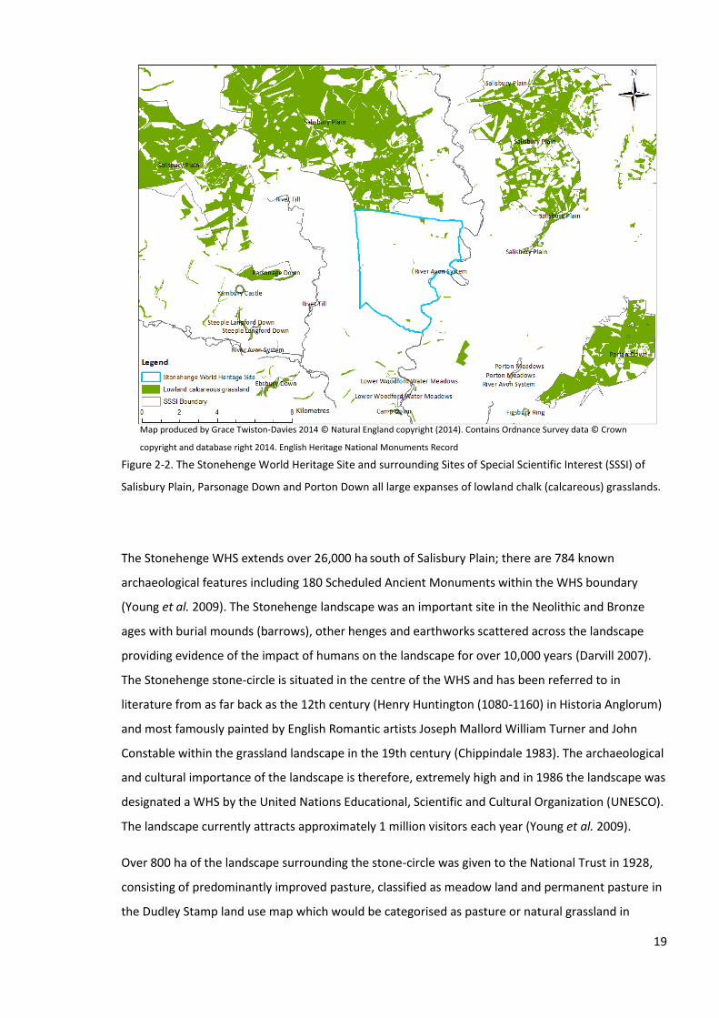
19
Figure 2-2. The Stonehenge World Heritage Site and surrounding Sites of Special Scientific Interest (SSSI) of
Salisbury Plain, Parsonage Down and Porton Down all large expanses of lowland chalk (calcareous) grasslands.
The Stonehenge WHS extends over 26,000 ha south of Salisbury Plain; there are 784 known
archaeological features including 180 Scheduled Ancient Monuments within the WHS boundary
(Young et al. 2009). The Stonehenge landscape was an important site in the Neolithic and Bronze
ages with burial mounds (barrows), other henges and earthworks scattered across the landscape
providing evidence of the impact of humans on the landscape for over 10,000 years (Darvill 2007).
The Stonehenge stone-circle is situated in the centre of the WHS and has been referred to in
literature from as far back as the 12th century (Henry Huntington (1080-1160) in Historia Anglorum)
and most famously painted by English Romantic artists Joseph Mallord William Turner and John
Constable within the grassland landscape in the 19th century (Chippindale 1983). The archaeological
and cultural importance of the landscape is therefore, extremely high and in 1986 the landscape was
designated a WHS by the United Nations Educational, Scientific and Cultural Organization (UNESCO).
The landscape currently attracts approximately 1 million visitors each year (Young et al. 2009).
Over 800 ha of the landscape surrounding the stone-circle was given to the National Trust in 1928,
consisting of predominantly improved pasture, classified as meadow land and permanent pasture in
the Dudley Stamp land use map which would be categorised as pasture or natural grassland in
Map produced by Grace Twiston-Davies 2014 © Natural England copyright (2014). Contains Ordnance Survey data © Crown
copyright and database right 2014. English Heritage National Monuments Record

20
Corine Land Cover (European Commission 2014), with small areas of arable land and fragments of
woodland (Figure 2-3). Since the beginning of the Second World War the Stonehenge landscape, as
well as the majority of the UK's permanent lowland semi-natural grassland, has been converted to
arable land or improved pasture and the little that remains is fragmented and mostly of low
conservation value (Fuller 1987; Hodgson et al. 2005). Semi-natural grasslands are defined as those
that have been modified by fertiliser or grazing for example, and where a high proportion of the
vegetation is a mixture of native grasses and herbs but woody shrubs are mostly absent. Improved
pasture is dominated by grasses with a low diversity of forb species and more than 50% Lolium
perenne, Trifolium repens or other agricultural species (Crofts & Jefferson 1999; JNCC 1990). By the
year 2000 the Stonehenge landscape was dominated by arable land and semi-improved pasture
which is defined as having a high diversity of forb species with less than 50% agricultural species and
not dominated by grasses and there were also (JNCC 1990) small fragments of chalk grassland and
woodland.
Figure 2-3. Land use map of the Stonehenge Landscape in the 1930's depicting the large expanse of permanent
grassland with small areas of arable land.

21
2.1.2 Plant and Lepidoptera nomenclature
Plant nomenclature for this study follows Stace (2010), New Flora of the British Isles Third edition
and Lepidoptera nomenclature follows Langmaid et al. (1989) The Butterflies of Great Britain and
Ireland: Hesperiidae to Nymphalidae and Heath & Emmet (1985) The Moths and Butterflies of Great
Britain and Ireland: Cossidae to Heliodinidae. In the field Lepidoptera were identified using Field
Studies Council Guide to the Butterflies of Britain and Guide to the day-flying moths of Britain .
2.1.3 Chalk grasslands
In the UK, calcareous grasslands are defined as existing on free-draining chalk or limestone soils. In
the UK National Vegetation Classification (NVC) the vegetation communities are referred to as
calcicolous or chalk grasslands and different types are dominated by Meadow Oat-grass (Avenula
pratensis), Downy Oat-grass (Avenula pubescens), Tor grass (Brachypodium pinnatum), Upright
Brome (Bromopsis erecta) and Sheep's Fescue (Festuca ovina) (Rodwell 1992). These types of
grassland are classified as semi-natural grasslands as they require management to maintain their
species diversity and to halt ecological succession. The most widespread and extensive chalk
grasslands in lowland southern UK are classified as either CG2, Festuca ovina-Avenula pratensis
dominated or CG3, Bromopsis erecta community (Rodwell 1992). There are currently up to 41,000
ha of lowland calcareous grassland in the UK which are distributed as large expanses and small
fragments, with large expanses across the South Downs in Hampshire and East Sussex and Salisbury
Plain in Wiltshire (Anon 1998). Across Salisbury Plain, Parsonage Down and Porton Down in Wiltshire
(Figure 2-4), there is approximately 15,000 ha accounting for around 30% of the UKs lowland
calcareous grassland (Natural England 2008).
Chalk grasslands were present in Europe in pre-Neolithic times as small isolated patches of natural
grasslands and have expanded, with the maximum spread apparent in Europe in the 14th-18th
centuries from large sheep flock-grazing (Poschlod & WallisDeVries 2002). In the last century, chalk
grasslands have declined in Europe from abandonment, conversion to arable land and afforestation
and are now threatened (Poschlod & WallisDeVries 2002). In the UK these types of semi-natural
lowland grasslands have declined by as much as 97% since World War II where intensive farming and
subsequent fragmentation has occurred (Fuller 1987; Hodgson et al. 2005). The majority of the
remaining lowland chalk grasslands have shifted to more mesotrophic conditions attributed to the
invasion of more competitive plant species and the local extinction of rarer calcicolous species as a
result of fragmentation and nitrogen enrichment (Bennie et al. 2006).

22
Chalk grasslands are Special Areas of Conservation (SACs), Sites of Special Scientific Interest (SSSI),
are included in the European Union legislation and the Habitats Directive as Biodiversity Action Plan
(BAP) priority habitat in the UK.
2.1.4 The Stonehenge World Heritage Site Management Plan
The Stonehenge WHS Management Plan was drafted in 2000 with the aims of extending the area of
permanent grassland to protect the archaeological features of the landscape from ploughing, to
restore the ecological and aesthetic value of the landscape and to provide open access areas for
visitors (Young et al. 2009). This landscape restoration project involved creating new species-rich
grasslands on ex-arable land which adjoined fragments of chalk grassland and increased the overall
area of permanent grassland and is henceforth referred to as grassland re-creation when referring to
individual fields (also grassland re-creation habitat patch) and restoration when referring to the
landscape scale project.
The Management Plan outlined aims for the restoration project and these were for the new
grasslands to be species-rich, based on local grassland community types and for natural regeneration
and development to be possible (Table 2-1). Guiding principles for management were provided to
achieve these aims and to enhance the nature conservation value of the grasslands and included:
sheep and cattle grazing regimes designed to encourage varied and selective grazing,
grazing and mowing to enhance the structural heterogeneity of grasslands to allow for
natural regeneration and colonisation,
seed dispersal enhanced from grazing and mowing regimes which allow time for seeds to
mature and disperse.
Table 2-1. Management aims or 'policies' relating to grassland and its impact on nature conservation from the
Stonehenge World Heritage Site Management Plan (Young et al. 2009).
Policy 3b Appropriate Agri-environment schemes should be maintained and developed to maximise the
protection of archaeological sites and their settings.
Policy 3f In the management of land in the future, permanent grasslands should be maintained,
enhanced and extended where appropriate.
Policy 3g The overall nature conservation value of the WHS should be maintained and enhanced, in
particular maintaining and improving the biodiversity of permanent grassland including the
existing limited areas of floristically rich chalk down-land turf, leading to greater diversity not
just of plants but also of birds and insects.
23
The grassland re-creation project required the collaboration and cooperation of a range of
stakeholders including the National Trust, English Heritage, the Royal Society for the Protection of
Birds (RSPB) and private landowners, with the tenant farmers committing to 10 years of the project
funded through Agri-environment schemes. From 2000-2005 tenant farmers entered into the
Avebury and Stonehenge Special Project Grant designed for the conservation and enhancement of
ancient monuments and received £120 per hectare of arable land that was changed to permanent
grassland. From 2005 onwards, tenant farmers entered in to a Higher Level Stewardship agreement
and were given £420 per hectare of arable land that was changed to permanent grassland
(Craythorne 2007). In 2000, seed was sourced from local species-rich chalk grassland on Salisbury
Plain Site of Special Scientific Interest (SSSI), approximately 5 km north-west of the Stonehenge
Landscape and sown in the first grassland re-creation field. From 2000 to 2012 a series of ex-arable
fields have been sown resulting in approximately 524 hectares of re-created grassland.
At the beginning of this study (2010), the landscape was a mosaic of chalk grassland fragments on
ancient burial mounds (barrows) and slopes, grassland re-creation fields of different ages since
sowing, semi-improved pasture, arable farmland and woodland (Figure 2-4). Fragments of chalk
grassland on slopes at Full-moon Bank and Luxenborough Bank (Figure 2-2) were considered as
target or reference habitat patches as they most resembled the donor habitat patch on Salisbury
Plain in terms of botanical characteristics with a chalk grassland community of (Bromopsis erecta,
CG3 community, Rodwell 1992, (Table 2-3).
These fragments contained a range of species characteristics of chalk grassland including grasses
Bromopsis erecta, Quaking Grass (Briza media) and herbs Small Scabious (Scabiosa columbaria),
Common Rock-rose (Helianthemum nummularium), Horseshoe Vetch (Hippocrepis comosa) and
Devil’s-bit Scabious (Succisa pratensis) (Allen & Brash 2008; Pemberton 2011). Smaller chalk
grassland fragments are also found at Cursus Barrows (Bromopsis erecta grassland community type)
and the small tussocky areas with ant hills at the Wintebourne Stoke Group of barrows and Fargo
Barrow, which were rabbit grazed and had Red Fescue (Festuca rubra), Hippocrepis comosa,
Helianthemum nummularium and Wild Thyme (Thymus polytrichus) (Avenula pubescens and
Brachypodium pinnatum grassland community types, CG6 and CG4, respectively (Pemberton 2011;
Twiston-Davies, Unpublished data). Groups of burial mounds at King Barrows and the Winterbourne
Stoke Group consisted of a mixture of chalk grassland species as listed above, as well as rough
grassland and shade tolerant species such as False Brome (Brachypodium sylvaticum), False Oat
Grass (Arrhenatherum elatius), Festuca ovina, Ground Ivy (Glechoma hederacea), Bird's-foot Trefoil
(Lotus corniculatus), Pyramidal Orchid (Anacamptis pyramidalis) and Greater Knapweed (Centaurea
scabiosa) (Allen & Brash 2008; Pemberton 2011; Twiston-Davies, Unpublished data). These were

24
both classified as a mosaic of Arrhenatherum elatius mesotrophic grassland, MG1 and Avenula
pubescens chalk grassland CG6 community types (Allen & Brash 2008; Rodwell 1992).
These chalk grassland fragments and barrow groups were managed by sheep or cattle grazing
depending on what livestock were in the adjacent field for a few weeks in the summer to control
scrub (Twiston-Davies, Unpublished data).
Figure 2-4. Map of the Stonehenge World Heritage Site (WHS), boundary of the National Trust owned lands
and land cover types in the year 2010 and the areas for grassland re-creation from 2000-2012.
Map produced by Grace Twiston-Davies 2013 © Natural England copyright (2013). Contains Ordnance Survey data © Crown copyright
and database right 2013. LCM2007 © and database right NERC (CEH) 2011. All rights reserved. © third party licensors. English
Heritage National Monuments Record

25
a. F
ull-
mo
on
Ban
k
b. L
uxe
nb
oro
ugh
ban
k
g. K
ing
Bar
row
s f.
Cu
rsu
s B
arro
ws
d. F
argo
Bar
row
c. W
inte
rbo
urn
e
e. W
inte
rbo
urn
e St
oke
Gro
up
h
i
j
k
l
m
n
o
p
Map
pro
du
ced
by
Gra
ce T
wis
ton
-Dav
ies
20
13
© N
atu
ral E
ngl
and
co
pyr
igh
t (2
01
3).
Co
nta
ins
Ord
nan
ce S
urv
ey d
ata
© C
row
n c
op
yrig
ht
and
dat
abas
e ri
ght
20
13
. LC
M2
00
7 ©
an
d d
atab
ase
righ
t N
ERC
(C
EH)
20
11
. All
righ
ts r
eser
ved
. © t
hir
d p
arty
lice
nso
rs.
26
Figure 2-5. The Stonehenge landscape in 2010 area owned and managed by the National Trust and fragments
of chalk (calcareous) grassland on slopes, a) Full-moon Bank, b) Luxenborough Bank, c) Winterbourne and on
burial mounds, d) Fargo Barrow, e) Winterbourne Stoke Group, f) Cursus Barrows, g) King Barrows. Fields for
grassland re-creation of different ages since sowing, h) Seven Barrows, i) Cuckoo Stone, j) Noice's Piece, k)
Stonehenge 05, l) Stonehenge 07 and m) Stonehenge 09. Grassland re-creation fields sown, o) in the year
2010, n) in the year 2011 and p) in the year 2012. Stonehenge stone-circle in the centre of the map.
2.1.5 Grassland re-creation technique
Seed was collected from the donor habitat patch using a brush harvester which is a specially
designed machine that harvests seed directly from wild meadows and grasslands and allows for the
seed to be processed and stored until it is sown at the receptor site (Edwards et al. 2007). Seed was
brush harvested in early August 2000 from Ministry of Defence (MOD) owned land on Salisbury Plain
SSSI (not within the area shown in Figure 2-4) classified as Bromopsis erecta grassland (in 1998, CG3
in the UK National Vegetation Classification; Rodwell 1992). In late August 2000, the seed was
applied (at a rate of 20 kg.ha-1) to Seven Barrows, the first grassland re-creation field. The seed was
mixed with fertiliser (at a rate of 222 kg.ha-1), using a phosphate fertiliser brand (Fibrophos 2014) in
order to aid the broadcasting of the seed. Although it is unusual to include fertiliser in the
restoration of low nutrient grassland, this low level of fertiliser was not considered likely to have
much impact on growth of vigorous species which would also be controlled by cutting (topping)
during the early years.
Seed sourced from the target or reference habitat patch is considered the best restoration
technique to establish similar plant communities (Prach et al. 2013; Pywell et al. 2002; Walker et al.
2004), but is also the most expensive technique (Toeroek et al. 2011). To increase cost effectiveness,
seed from this first re-creation field, Seven Barrows, was brush harvested in July 2002 and sown in
further grassland re-creation fields at the end of the summer in 2002, 2003, 2005 and 2007 and all
excess seed was stored for future re-creation. For the 2010, 2011 and 2012 re-creation fields, seed
was brush-harvested from the 2003 Normanton Gorse and Noice's Piece fields.
The difference in seed source, either from Salisbury Plain, Seven Barrows field or the 2003
restoration fields will have an impact on the subsequent plant community that will establish due to
different original community types (Table2-3, Figure 2-6) and the seed dilution effect. For example,
as much as 30% of seed transferred from a donor to the receptor habitat patch will not be viable
(Kiehl et al. 2006). Additionally the available seed bank and soil nutrient conditions of the receptor
patch and its proximity to other sources of seed will also affect the subsequent plant community
type (Fagan et al. 2008; Fagan et al. 2010). Results of plant surveys across the landscape over a four

27
year period to investigate the progression of the restoration project and disseminate some of these
differences are described in section 2.1.6.
The management of the grassland re-creation fields after sowing included mechanical topping two
or three times a year in the first two years to control weeds followed by a late summer hay cut and
autumn grazing with cattle or sheep. The precise management regimes that were applied differed
between fields depending on the tenant farmers' preferences and are summarised below Table 2-2).
Table 2-2. Grassland re-creation field management (Twiston-Davies Unpublished data; Campbell 2009;
Craythorne 2007; Pemberton 2011). Grazing intensity is no. of livestock units per hectare per year (LU/ha/Yr).
Fields Year
sown
Mowing Grazing
Seven Barrows 2000 Topping to control weeds in the first 2
years. Brush harvesting in years 2, 3, 5, 7
and 9 in July or August.
No grazing in the first 2 years. Autumn
sheep grazing from years 3-5. Summer
grazing year 6, no grazing in year 7.
Sheep grazing from year 8 onwards
(approx 130 ewes and lambs a year).
Cuckoo Stone 2002 Topping to control weeds in the first 2
years and in subsequent years if weedy
species became dominant or grasses
were too large and unpalatable. Hay cut
year 5 early August and in year 6.
High density cattle grazing April-June in
years 2-4, No grazing in year 5 or 6.
Sheep grazing 6 weeks in July and 2-3
weeks in Sept year 9 and onwards
(Grazing density unknown).
Noice's Piece 2003 Topping to control weeds in the first 2
years. Hay cut late September in year 4
and brush harvested in year 6 and 7.
Grazed after 2 years. Cattle grazing
from years 2-6. No grazing 2010
onwards (0.6-0.75 LU/ha/yr).
Stonehenge 05 2005 Topping to control weeds in the first 2
years and subsequently if weedy species
became dominant or grasses too large
and unpalatable. Topped early July and
September year 2. Hay cut June/July
year 4 and onwards.
Cattle grazed from year 2 onwards (0.6-
0.75 LU/ha/yr).
Stonehenge 07 2007 Topping to control weeds in the first 2
years.
Cattle grazed from year 2 onwards (0.6-
0.75 LU/ha/yr).
Stonehenge 09 2009 Topping to control weeds in the first 2
years in June/ July.
Cattle grazed from year 2 onwards (0.6-
0.75 LU/ha/yr).

28
2.1.6 Botanical characteristics of the re-creation grasslands
Botanical surveys of the grassland re-creation fields were conducted in 2007, 2009 and 2011
(Campbell 2009; Craythorne 2007; Pemberton 2011). The most recent survey showed that for most
of the re-creation grassland fields the highest similarity was with mesotrophic grassland
communities of the NVC (Pemberton 2011; Twiston-Davies et al. in press) determined by comparing
the species and abundance using floristic tables (Rodwell 1992) and using MAVIS Plot analyzer 1.0 to
calculate Czekanowski coefficient (Smart 2001). The first grassland re-creation field, Seven Barrows
(sown in 2000 with seed brush harvested from a nearby donor habitat patch) was more similar to
the chalk grassland reference community Bromopsis erecta grassland; Knautia arvensis-Bellis
perennis sub community (Rodwell 1992). Other re-creation fields sown in 2003, 2004 and 2005 with
seed brush harvested from Seven Barrows showed transitional mesotrophic/calcicolous grassland
vegetation characteristics of Cynosurus cristatus-Centaurea nigra/Bromopsis erecta communities
(Pemberton 2011; Twiston-Davies et al. in press). Seven Barrows restoration field had reached
similar botanical conditions to the target habitat within seven years with the plant community type
most associated with chalk CG3 (NVC, Rodwell 1992) although with a much lower similarity than the
target habitat patch. However, the 20003 restoration fields after seven years had transitional
chalk/mesotrophic community types (Table 2-3, Figure 2-6). This suggests that seed sourced from
the Seven Barrows restoration field may result in transitional chalk/mesotrophic grassland
characteristics and not fully reach the botanical conditions of the original donor habitat patch,
although this hypothesis can only be tested given more time for the younger fields to mature.
Younger grassland re-creation fields sown since 2007 showed similarities with mesotrophic grassland
communities of Arrhenatherum elatius, Lolium perenne-Cynosurus cristatus or open vegetation
Matricaria perforata-Stellaria media.
Many of the grassland re-creation fields had characteristic chalk grassland species but not all in the
abundances required for it to be classified as chalk grassland community types for example, grasses
Bromopsis erecta and Briza media were present in all grassland re-creation fields and herbs
Hippocrepiss comosa in Cuckoo Stone and Stonehenge 05 (Craythorne 2007) and Helianthemum
nummularium in Seven Barrows (Campbell 2009). The lack of these species in the 2011 surveys may
have been due to just ten 2m by 2m quadrats being used to survey each field, which was much lower
than the one quadrat per hectare in 2009 (minimum 12) and 1.5 per hectare in 2007 (minimum 18)
(Campbell 2009; Craythorne 2007; Pemberton 2011).
Figure 2-6 shows the similarity of grassland re-creation habitat patches (fields) with chalk grassland
from botanical surveys in 2007, 2009 and 2011 (Campbell 2009; Craythorne 2007; Pemberton 2011).
As the grassland matures the similarity with chalk grassland increases. The similarity of the species-
rich grassland donor habitat patch to a NVC chalk grassland vegetation community was 68% (in

29
1998) and the reference fragment at the Stonehenge landscape at was 66% (in 2011) in the Seven
Barrows grassland re-creation field sown in the year 2000 and recorded in 2011 was 57%. This
indicates that within a decade the grassland re-creation fields are reaching similar botanical
conditions to the target habitat but they have lower percentage similarity to chalk grassland
community type (CG3 in NVC) than the target habitats.
Seed harvested from a target habitat patch is one of the best methods for achieving plant
communities similar to the target habitat patch. However, these results suggest that seed harvested
from young restoration which is only three years old can provide species-rich grassland with some
target species characteristic of the target habitat patch even if it doesn't have the same community
classification of the target habitat patch (Twiston-Davies et al. in press). This is a lower cost option
for a large landscape scale projects and can provide incentives to farmers to manage restoration
land in order to sell the seed for other projects. Differences between the established communities
depending on their seed source is difficult to evaluate within the short time period of the
Stonehenge restoration landscape, but would be possible for example, after the 2009 field sown
with seed sourced from 2003 fields had reached a decade in age.
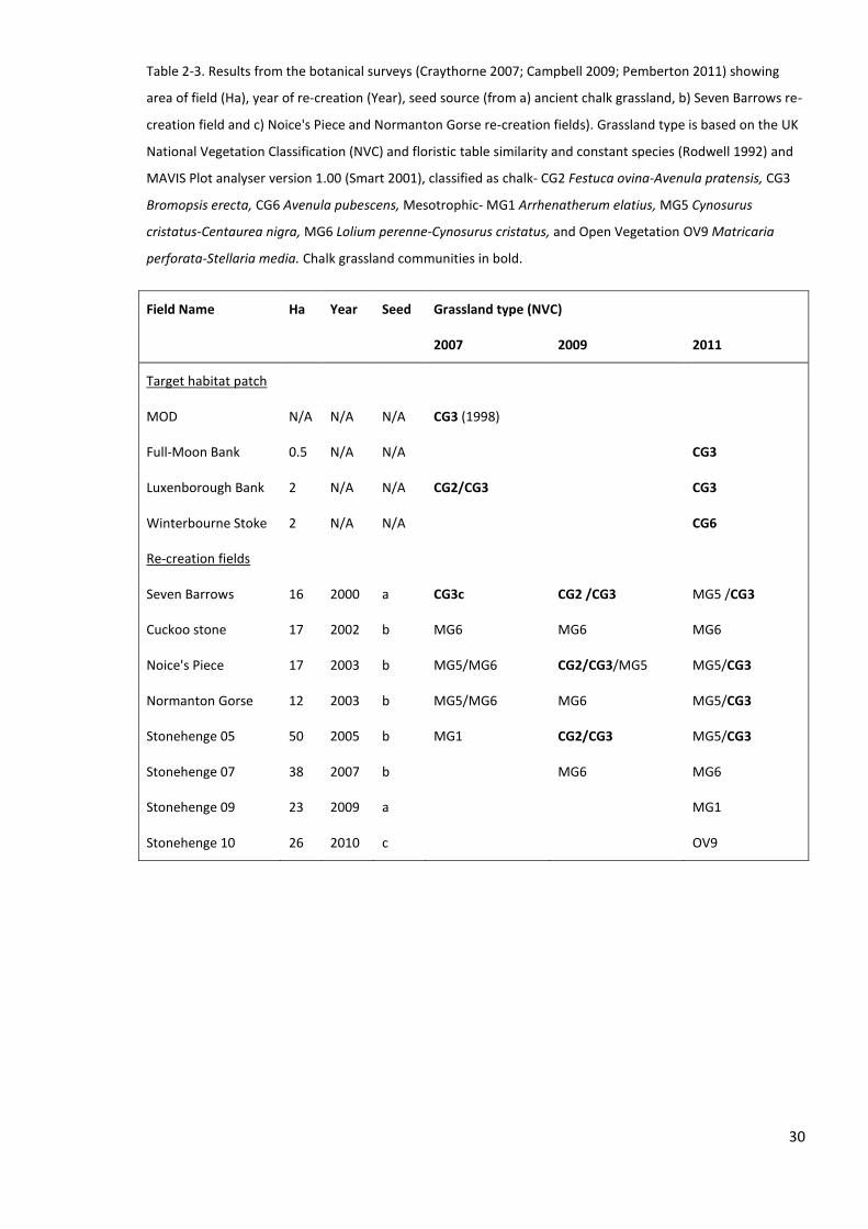
30
Table 2-3. Results from the botanical surveys (Craythorne 2007; Campbell 2009; Pemberton 2011) showing
area of field (Ha), year of re-creation (Year), seed source (from a) ancient chalk grassland, b) Seven Barrows re-
creation field and c) Noice's Piece and Normanton Gorse re-creation fields). Grassland type is based on the UK
National Vegetation Classification (NVC) and floristic table similarity and constant species (Rodwell 1992) and
MAVIS Plot analyser version 1.00 (Smart 2001), classified as chalk- CG2 Festuca ovina-Avenula pratensis, CG3
Bromopsis erecta, CG6 Avenula pubescens, Mesotrophic- MG1 Arrhenatherum elatius, MG5 Cynosurus
cristatus-Centaurea nigra, MG6 Lolium perenne-Cynosurus cristatus, and Open Vegetation OV9 Matricaria
perforata-Stellaria media. Chalk grassland communities in bold.
Field Name Ha Year Seed Grassland type (NVC)
2007 2009 2011
Target habitat patch
MOD N/A N/A N/A CG3 (1998)
Full-Moon Bank 0.5 N/A N/A CG3
Luxenborough Bank 2 N/A N/A CG2/CG3 CG3
Winterbourne Stoke 2 N/A N/A CG6
Re-creation fields
Seven Barrows 16 2000 a CG3c CG2 /CG3 MG5 /CG3
Cuckoo stone 17 2002 b MG6 MG6 MG6
Noice's Piece 17 2003 b MG5/MG6 CG2/CG3/MG5 MG5/CG3
Normanton Gorse 12 2003 b MG5/MG6 MG6 MG5/CG3
Stonehenge 05 50 2005 b MG1 CG2/CG3 MG5/CG3
Stonehenge 07 38 2007 b MG6 MG6
Stonehenge 09 23 2009 a MG1
Stonehenge 10 26 2010 c OV9
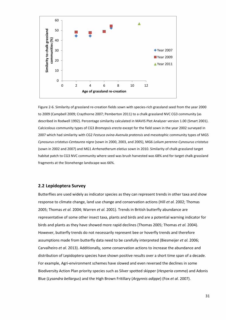
31
Figure 2-6. Similarity of grassland re-creation fields sown with species-rich grassland seed from the year 2000
to 2009 (Campbell 2009; Craythorne 2007; Pemberton 2011) to a chalk grassland NVC CG3 community (as
described in Rodwell 1992). Percentage similarity calculated in MAVIS Plot Analyser version 1.00 (Smart 2001).
Calcicolous community types of CG3 Bromopsis erecta except for the field sown in the year 2002 surveyed in
2007 which had similarity with CG2 Festuca ovina-Avenula pratensis and mesotophic community types of MG5
Cynosurus cristatus-Centaurea nigra (sown in 2000, 2003, and 2005), MG6 Lolium perenne-Cynosurus cristatus
(sown in 2002 and 2007) and MG1 Arrhenatherum elatius sown in 2010. Similarity of chalk grassland target
habitat patch to CG3 NVC community where seed was brush harvested was 68% and for target chalk grassland
fragments at the Stonehenge landscape was 66%.
2.2 Lepidoptera Survey
Butterflies are used widely as indicator species as they can represent trends in other taxa and show
response to climate change, land use change and conservation actions (Hill et al. 2002; Thomas
2005; Thomas et al. 2004; Warren et al. 2001). Trends in British butterfly abundance are
representative of some other insect taxa, plants and birds and are a potential warning indicator for
birds and plants as they have showed more rapid declines (Thomas 2005; Thomas et al. 2004).
However, butterfly trends do not necessarily represent bee or hoverfly trends and therefore
assumptions made from butterfly data need to be carefully interpreted (Biesmeijer et al. 2006;
Carvalheiro et al. 2013). Additionally, some conservation actions to increase the abundance and
distribution of Lepidoptera species have shown positive results over a short time span of a decade.
For example, Agri-environment schemes have slowed and even reversed the declines in some
Biodiversity Action Plan priority species such as Silver spotted skipper (Hesperia comma) and Adonis
Blue (Lysandra bellargus) and the High Brown Fritillary (Argynnis adippe) (Fox et al. 2007).
0
10
20
30
40
50
60
0 2 4 6 8 10 12
Sim
ilari
ty t
o c
hal
k gr
assl
and
co
mm
un
itie
s (%
)
Age of grassland re-creation
Year 2007
Year 2009
Year 2011

32
All Lepidoptera transect (Chapter 3) and behaviour surveys (Chapters 4 and 5) were conducted in
suitable conditions and methods adapted from the Butterfly Monitoring Scheme (Pollard & Yates
1993) between 10am-5pm on dry days with a wind speed less than Beaufort scale 5, a temperature
of more than 13 C on days with 60% sunshine or more than 17 C when overcast.
Lepidoptera were identified using Field Studies Council guides for butterflies and day flying moths of
Britain (1998 and 2006, respectively, nomenclature follows Heath & Emmet 1985; Langmaid et al.
1989) and close-focus binoculars when required. If Lepidoptera were feeding on nectar, the species
of plant was identified (nomenclature follows Stace Third edition, 2010).
For the distributions of Lepidoptera distributions in the wider landscape used in Chapter 3, data
were provided from the Butterflies for the New Millennium recording scheme, courtesy of Butterfly
Conservation and the Wiltshire and Swindon Biological Records Centre.
2.2.1 Species ecological groups and mobility group
The butterflies surveyed were grouped using ecological classifications of species associated with: a)
ruderal vegetation, b) short-grass herb-rich vegetation, c) open grassland with medium to tall sward
or warm open grassland with short-sward and, c) woodland (Shreeve et al. 2001). The difference
between the two grassland ecological groups was that those associated with short-grass herb-rich
vegetation were not dependant on grasses for any part of their life-cycle, whereas, those associated
with short, medium or tall warm open grassland were (Shreeve et al. 2001). The larval host plants of
the herb-rich grasslands associated group were Legumes and they were likely to have a symbiotic
relationship with ants. The ruderal-vegetation group is not associated with a particular family of
larval host plants, but is likely to be associated with tall and/or mature herbs and to overwinter as
pupae. These categories are based on a Principal Component Analysis based on the ecological
attributes at all stages of the Lepidoptera life cycle, with the defined groups differing mostly in
range, distribution, biotope range, dispersal ability and recent declines in abundance between
groups (Shreeve et al. 2001).
Day flying moths were categorised based on their association with different habitat types: the Six-
spot Burnet (Zygaena filipendulae) was more associated with herb-rich grassland as its larval host
plant is legume species Lotus corniculatus, (although this species will use tall grass stems and
pupation sites), the Forester moth (Adscita statices) as it is associated with herb-rich chalk grassland
where its larval host plant Common Rock-rose (Helianthemum nummularium) is abundant (Heath &
Emmet 1985). Both of these moth species were also categorised as sedentary in mobility (Naumann
et al. 1999). The Hummingbird Hawk moth (Macroglossum stellatarum) was categorised as
associated with ruderal vegetation as it is a widespread immigrant species associated with a variety
of habitat types (Heath & Emmet 1985; Langmaid et al. 1989).

33
Mobility groups were of widespread, intermediate and sedentary groups which are estimated using
a mark and recapture study and represent emigration rates and colonisation distances as described
in Pollard & Yates (1993), this is a widely used but relatively coarse classification whereby mobility
categories are an assumption and likely to be an underestimate mobility. Species categorised as
sedentary are unlikely to move outside the habitat patch and are considered to have a closed
population structure, whereas, species categorised as widespread are wide-ranging and frequently
move between habitat patches and have an open population structure. species categorised as
intermediate are somewhere in-between sedentary and widespread. Other mobility categories are
availably such as Bink (1992) which has nine mobility categories as well as Cowley et al. (2001) and
Komonen et al. (2004) which are continuous index value based on questionnaires to experts.
However, all of these measures were significantly strongly positively correlated (Komonen et al.
2004) and therefore the most simple measure of three categories by Pollard and Yates (1993) is used
for this study.
2.3 Habitat quality
Habitat quality was recorded using the number and species of nectar flowers and vegetation
characteristics in the habitat fragments and the wider landscape to include both the habitat and
matrix resource measures as not all resources occur in the defined 'habitat' of an individual (Dennis
et al. 2003; Ouin et al. 2004).
Habitat quality, in terms of the number of nectar resources (flowering units)and vegetation
characteristics was measured for transect surveys in Chapter 3 and boundary behaviour surveys in
Chapters 4 and 5 using quadrats measuring 0.5 m by 0.5 m. Nectar resources were measured by the
total number, family and individual species densities of flowering units that Lepidoptera use for
nectar sources (Hardy et al. 2007). The availability of nectar plants was measured as this resource is
used by both male and female Lepidoptera. Other habitat characteristics measured included the
vegetation height and density (using the drop disc method, Stewart et al. 2001), percentage
coverage of bare ground and dead vegetation and the heterogeneity of these variables (calculated
as the Coefficient of Variation).
Variables relating to vegetation height and density and the coverage of bare ground and leaf litter
are important for butterflies, as they effect the microclimate and can be used as a resource for
oviposition, pupation, courtship and thermoregulation (Beyer & Schultz 2010; Lawson et al. 2014;
NCC 1986; Thomas et al. 2009). Different butterfly species are associated with different vegetation
heights (NCC 1986) for example, the recovery of a threatened Butterfly species, the Large Blue
(Maculinea arion) can be determined by the vegetation height as this effects the microclimate and

34
the subsequent establishment of a successful symbiotic relationship with the Myrmica sabuleti ant
species which prefers warmer microclimate when there is a shorter (Thomas et al. 2009). The cover
and height of grasses and depth of leaf litter can determine the selection of oviposition sites for
Skipper species (Pokes mardon) (Beyer & Schultz 2010) and in cooler sites, bare ground may provide
a warmer microclimate for oviposition site for Heperia comma (Lawson et al. 2014).
Vegetation surveys that were conducted prior to Lepidoptera surveys (Campbell 2009; Craythorne
2007; Pemberton 2011) provided detailed species lists to determine the presence of larval host
plants in grassland re-creation fields and chalk grassland fragments (Table 2-4).
Table 2-4. List of host plants for Lepidoptera species associated with grasslands or ruderal vegetation (Hardy et
al. 2007; Shreeve et al. 2001).
Larval host plant Lepidoptera species
Grasses
Common Bent (Agrostis
capillaris)
Meadow Brown (Maniola jurtina), Gatekeeper (Pyronia tithonus),
Small Heath (Coenonympha pamphilus)
Creeping Bent (Agrostis
stolonifera)
Ringlet (Aphantopus hyperantus), Meadow Brown (Maniola
jurtina), Gatekeeper (Pyronia tithonus), Small Heath
(Coenonympha pamphilus)
Cock's Foot (Dactylis
glomerata)
Essex Skipper (Thymelicus lineola), Marbled White (Melanargia
galathea), Ringlet (Aphantopus hyperantus), Gatekeeper (Pyronia
tithonus)
Sheep's Fescue (Festuca
ovina)
Marbled White (Melanargia galathea), Meadow Brown (Maniola
jurtina), Gatekeeper (Pyronia tithonus), Small Heath
(Coenonympha pamphilus)
Meadow Fescue (Festuca
pratensis)
Gatekeeper (Pyronia tithonus)
Red Fescue (Festuca rubra) Marbled White (Melanargia galathea), Gatekeeper (Pyronia
tithonus)
Yorkshire Fog (Holcus lanatus) Small Skipper (Thymelicus sylvestris), Meadow Brown (Maniola
jurtina)
Perennial Ryegrass (Lolium
perenne)
Meadow Brown (Maniola jurtina)
Essex Skipper (Thymelicus lineola), Small Skipper(Thymelicus

35
Timothy Grass (Phleum
pratense)
sylvestris), Marbled White (Melanargia galathea)
Smooth Meadow Grass (Poa
pratensis)
Ringlet (Aphantopus hyperantus) , Meadow Brown (Maniola
jurtina), Gatekeeper (Pyronia tithonus), Small Heath
(Coenonympha pamphilus)
Rough Meadow Grass (Poa
trivialis)
Meadow Brown (Maniola jurtina), Gatekeeper (Pyronia tithonus),
Small Heath (Coenonympha pamphilus)
Herbs
Cuckoo Flower (Cardamine
pratensis)
Green-veined White (Pieris napi)
Common Rock-rose
(Helianthemum
nummularium)
Brown Argus (Arica agestis)
Horseshoe Vetch (Hippocrepis
comosa)
Adonis Blue (Lysandra bellargus)
Bird's-foot Trefoil (Lotus
corniculatus)
Chalkhill Blue (Lysandra coridon), Clouded Yellow (Colias croceus),
Six-spot Burnet (Zygaena filipendulae)
Lesser Hop Trefoil (Trifolium
dubium)
Chalkhill Blue (Lysandra coridon), Clouded Yellow (Colias croceus)
Red Clover (Trifolium
pratense)
Chalkhill Blue (Lysandra coridon), Clouded Yellow (Colias croceus)
White Clover (Trifolium
repens)
Chalkhill Blue (Lysandra coridon), Clouded Yellow (Colias croceus),
Common Nettle (Urtica dioica) Small Tortoiseshell (Aglais urticae), Red Admiral (Vanessa
atalanta)
The average weather conditions to the nearest hour of survey time were also recorded from the
closest Meteorological station at Boscombe Down, Amesbury, Wiltshire (approximately 6.5 km WSW
from the stone-circle, British National Grid reference SU 17763 39246). For the boundary behaviour
experiment detailed in Chapter 5, the average microclimate conditions of humidity, wind speed and
air temperature were recorded using a digital hand held recorder held one metre from the ground
for three minutes at the start of the survey.

36
2.4 Mapping the Stonehenge WHS and the wider landscape
An Ordnance Survey Mastermap Topology layer of the Stonehenge World Heritage Site and a buffer
of 1 km of its boundary was obtained from EDINA (Ordnance Survey Mastermap 2010, EDINA
Digimap 1: 1250 scale) in polygon format and edited in ArcMap (version 10.1 ESRI©) to include the
small fragments of chalk grassland, the classification of linear features (road verges, track verges and
field margins) and other un-classified polygons using personal knowledge, Google Earth©, Land
Cover Map 2007 and the Stonehenge World Heritage Site Management Plan (Morton et al. 2011;
Young et al. 2009). For this map the minimum mapable unit was 0.25 ha. This map was used in
Chapter 3 to calculate different land cover types and features in buffers around Lepidoptera transect
using ArcMap (version 10.1 ESRI©).
Land Cover MAP 2007 data was sourced from the Centre for Ecology and Hydrology, consisting of
broad habitat types at 25 m by 25 m raster grid square resolution (Land Cover Map 2007, Table 2-5,
Morton et al. 2011). These were edited to represent the land cover types in the landscape prior to
grassland re-creation in 2000, and in 2012 after the last grassland re-creation fields had been sown
with an additional category of grassland re-creation, based on Stonehenge World Heritage Site
Management Plans (Young et al. 2009) and personal observations (Figure 2-7). Grassland re-creation
areas that were sown with species-rich seed mixtures prior to 2007 were classed as either improved
grassland or neutral grassland in Land Cover Map 20007 and so were edited to be classed as arable
and horticulture in 2000 and to be classed as re-creation grasslands in 2012. Grassland re-creation
areas sown in and after 2007 were classed as arable and horticulture in Land Cover Map 2007 and so
were edited to be classed as re-creation grassland in 2012.

37
Table 2-5. Land Cover Map 2007 habitat types and description. Ex arable fields that were sown with species-
rich grassland seed mixtures between 2000-2012 were classed as re-creation grassland.
Land Cover Map Description
Broadleaved Woodland Broadleaved, mixed and yew woodland with stands >5m high and tree cover
>20%.
Coniferous Woodland Semi-natural stands and plantations with cover >20%.
Arable and Horticulture Includes annual crops, perennial crops (e.g. orchards) and freshly ploughed
land
Improved Grassland Higher productivity distinguished improved grasslands from the other
categories as well as the lack of winter senescence
Neutral Grassland Determined by botanical composition
Calcareous Grassland As above but often mis-classified as improved grassland
Rough Grassland Mix of areas managed, low productivity grassland and some semi-natural
which could not be assigned acid, neutral or calcareous
Freshwater Standing open water, canals, rivers and streams
Urban Dense urban, town and city centres with little vegetation also docks, car
parks and industrial estates
Suburban Includes urban area with vegetation
GIS layers of the Lowland Calcareous Grasslands were obtained from Natural England (MAGIC,
Natural England 2010) in polygon format (data from 1998-2001) and edited to include the additional
fragments at the Stonehenge Landscape on slopes and burial mounds (Winterbourne Stoke Group,
Fargo Barrow, Full-moon Bank and Luxenborough Bank). These fragments were too small to be
categorised by the Lowland Calcareous Grassland survey (less than 25m by 25m n area). The new
Lowland Calcareous Grassland layer was combined with the edited Land Cover Maps 2007 layer as
the Lowland Calcareous Grassland Survey was more accurate at identifying chalk grassland than the
Land Cover Map 2007. The Sites of Special Scientific Interest and World Heritage Site boundaries
were obtained from Natural England (MAGIC, Natural England and English Heritage 2010) and the
National Trust Boundary was digitised by hand from maps in Young et al. (2009).

38
Figure 2-7. Outline of method for creating grassland habitat network maps using Land Cover Map 2007
(Morton et al. 2011) and Lowland Calcareous Grassland map (1998-2001), edited to represent the Stonehenge
World Heritage Site in 2000, 2010 and 2012.
All maps in this thesis are produced using ArcGIS© software by ESRI and contain the copyright
information from the data sources. All diagrams are created using Microsoft Word©. All graphs are
created using Microsoft Excel © and all ordination diagrams using CanoDraw© for CANOCO 5 ©.
Land Cover Map 2007 (LCM07) Lowland Calcareous Grassland (LCG) map
Edited to include WHS
grassland re-creation
Edited to include chalk
grassland fragments within WHS
Union of LCM07 and LCG
Classify remaining LCM07 chalk
grassland as neutral grassland
Grassland network
2012 (Chapter 6)
Grassland network
2000 (Chapter 6)

39
Chapter 3 Landscape scale grassland restoration at the Stonehenge World
Heritage Site, UK: Lepidoptera biodiversity enhancement?
3.1 Introduction
Habitat restoration at the landscape scale has the potential to create new habitats, expand and
buffer existing habitat fragments, increase the permeability of the intervening matrix and act as
stepping stones and corridors through the landscape (Pfadenhauer 2001). Landscape restoration
science is however, a relatively new discipline with a lack of studies that translate evidence-based
research into policy and explicit management recommendations for landscape scale projects
(Brudvig 2011; Menz et al. 2013; Young et al. 2005).
Habitat restoration using regional seed mixtures has been utilised to restore botanically species-rich
grasslands (Mitchley et al. 2012; Prach et al. 2013; Pywell et al. 2002; Walker et al. 2004) and the
strength of restoration science lies in this focus on restoring flora communities (Young 2000; Young
et al. 2005). The restoration of fauna is not necessarily guaranteed (Cristescu et al. 2013), and yet it
is vital to restore biodiversity and ecological interactions. This is especially crucial in species-rich
grassland such as calcareous grasslands, which have high biodiversity value in Europe (van Swaay
2002; WallisDeVries et al. 2002) and a third of semi-natural dry grassland in the Atlantic Europe
region of the Natura 2000 network in are in the UK (Calaclura & Spinell 2008).
Measuring the biodiversity enhancement as a result of habitat restoration for invertebrates is
complex as their different functional, ecological and mobility groups can determine their response to
habitats under restoration and the landscape (Batary et al. 2012; Dover & Settele 2009; Tscharntke
& Brandl 2004; Woodcock et al. 2012b). Therefore, it is crucial to understand, interpret and predict
these differences and complex interactions of invertebrates to habitat and landscape modification
(Dennis et al. 2004; Diamond et al. 2011; Hardy et al. 2007).
The relative importance of landscape characteristics and configuration compared with habitat patch
characteristics are much debated. Habitat patch connectivity is considered by some, as crucial as
habitat extent and quality (Doerr et al. 2011; Prugh et al. 2008) and in agricultural landscapes non-
habitat features such as the intervening matrix and linear features (for example, field margins and
hedges) provide resources and enhance landscape connectivity (Delattre et al. 2010b; Ouin et al.
2004). Additionally, landscape complexity and heterogeneity (diversity of habitat types and
structure) can be as important as habitat patch characteristics for conservation especially for the
40
majority of species for example, butterflies and other pollinators (Batary et al. 2011; Shreeve &
Dennis 2011).
The influence of the surrounding landscape and intervening matrix is arguably less important than
the effects of the area, extent or isolation of habitat patches (Hodgson et al. 2011; Hodgson et al.
2009; Prevedello & Vieira 2010). This means that investigating the relative contribution of both the
habitat and landscape characteristics is necessary to assign appropriate restoration site targeting
and for the subsequent management of these sites.
As part of the Stonehenge World Heritage Site (WHS) Management Plan, over 500 hectares of
species-rich grassland are currently being restored and re-created on ex-arable fields in Wiltshire,
UK, using species-rich, locally sourced seed mixtures from a donor habitat patch. Fields that were
sown with this seed mix are henceforth referred to as grassland re-creation fields. The aim of this
restoration project is to re-connect the isolated fragments of ancient chalk grassland to the wider
landscape. The project also provides an opportunity to investigate the ecological benefits of
landscape restoration and the landscape factors and identify species traits that may facilitate or
impede the re-colonisation of newly created habitats.
Previous surveys of the botanical characteristics of this restoration project have shown that the
grassland re-creation fields have reached similar ecological conditions of the donor habitat patch
within 7-10 years (Campbell 2009; Pemberton 2011), a time-span that is supported by other studies
(Piqueray et al. 2011; Prach et al. 2013). However, for some species-rich grassland restoration
projects it can take decades to reach the precise botanical conditions of the donor habitat patch
(Fagan et al. 2008).
Butterflies are used as an indicator group to evaluate the biodiversity enhancement of the
restoration project as they respond quickly to environmental and land use changes (Hill et al. 2002;
Warren et al. 2001), can reflect trends in other taxa (Thomas et al. 2004), and are especially suited
for short term restoration measures in calcareous grasslands (Rakosy & Schmitt 2011). However,
trends in UK Lepidoptera do not always represent those in other taxa, for example they do not
necessarily reflect trends in bees and may not be representative of other EU countries (Biesmeijer et
al. 2006; Carvalheiro et al. 2013).

41
3.2 Aims and Hypotheses
Aims;
To evaluate the biodiversity enhancement of grassland restoration and re-creation at the
habitat patch and landscape scales using Lepidoptera density, diversity and community
compositions as biodiversity indicators in re-created fields and reference habitat patches.
To investigate the habitat and landscape characteristics that encourage the colonisation of
new habitats and the movement of taxa from isolated chalk grassland fragments.
To determine the role of species traits in the colonisation of new habitats and the
movement of species from isolated chalk grassland fragments.
Hypotheses;
i. Re-creation grassland habitat patches with vegetation structure and nectar resources similar
to the reference habitat will have higher Lepidoptera species richness and abundance than
those that do not
ii. Re-creation grassland habitat patches that are more structurally connected as measured by
the amount of surrounding linear features will have higher Lepidoptera species richness and
abundance tan those that do not.
iii. Older grassland re-creation patches will have higher species richness and abundance and be
more similar to reference grasslands in community assemblage than newer habitat patches.
iv. Lepidoptera associated with grassland habitats will be an effective indicator of the effect of
restoration measures on biodiversity.
v. Species traits will be significant in determining the colonisation of new habitats and the
movement of species from isolated chalk grassland fragments.
vi. Species that use grasses as larval-host plants will colonise re-creation grasslands faster than
those with specialist herb larval host-plants.
vii. More mobile species will colonise re-creation grasslands faster compared to those with low
mobility.
3.3 Materials and Methods
3.3.1 Study site
The study site was the National Trusts' Stonehenge landscape within the Stonehenge WHS in
Wiltshire, South-West UK, where a long term landscape scale grassland restoration and re-creation
project has been underway. In the year 2000, seed was brush harvested from a nearby calcareous
grassland donor habitat patches on Salisbury Plain, (NW of the Stonehenge Landscape) and used to

42
establish new grassland on ex-arable fields until 2012 (Chapter 2). The aim of this was to protect the
archaeological features across the landscape and to restore the aesthetic and ecological value of the
landscape (Young et al. 2009).
During this study (2010-2011) the landscape consisted of a mosaic of chalk grassland fragments on
ancient burial mounds (barrows) and slopes, grassland re-creation fields of different ages since
sowing, semi-improved pasture, arable farmland and woodland (Figure 3-1).
Figure 3-1. Land cover types and sites for surveys in The National Trusts' Stonehenge Landscape boundary.
Fragments of chalk (calcareous) grassland on slopes: a) Full-moon Bank, b) Luxenborough Bank, c)
Winterbourne and d) Fargo Barrow) and barrow groups, e) Winterbourne Stoke Group, f) Cursus Barrows and
g) King Barrows. Grassland re-creation of different ages since sowing from 2000-2009, h) Seven Barrows, i)
Cuckoo Stone, j) Noice's Piece, k) Stonehenge 05, l) Stonehenge 07 and m) Stonehenge 09. Stonehenge stone-
circle situated in the centre of the map.
3.3.2 Lepidoptera surveys
All survey were carried out on the National Trust owned land of the Stonehenge World Heritage Site
using transect survey methods adapted from the Butterfly Monitoring Scheme (Pollard & Yates
1993, Chapter 2). During the survey, the researcher walked along the transect at a slow, steady pace
allowing five minutes for each 20 m section of transect and recorded the number and species of
Map produced by Grace Twiston-Davies 2013 © Natural England copyright (2013). Contains Ordnance Survey data © Crown copyright
and database right 2013. LCM2007 © and database right NERC (CEH) 2011. All rights reserved. © third party licensors.

43
Lepidoptera present 5 m either side and ahead. If Lepidoptera were observed feeding, then the
nectar plant species was also recorded.
Habitat transect surveys were carried out from June to September 2010 using 17, 200 m long
transects located in the centre of different grassland re-creation fields of different ages since sowing
and broad habitat types; re-created grassland sown in the years 2000, 2002 and 2003 (older re-
creation collectively), re-created grassland sown in the years 2005, 2007 and 2009 (newer re-
creation collectively), arable land (bare ground at the time), chalk grassland fragments on slopes
(reference habitat) and on ancient burial mounds (barrows) and semi-improved pasture (adjacent to
chalk grassland fragments on barrows) (Figure 3-1, Table 3-1). Transects were surveyed on three
occasions spread across the field season, and throughout the day and were selected ad-hoc for
survey in order to minimise the effect that the time of year and day would have on results.
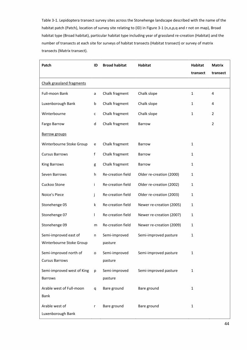
44
Table 3-1. Lepidoptera transect survey sites across the Stonehenge landscape described with the name of the
habitat patch (Patch), location of survey site relating to (ID) in Figure 3-1 (n,o,p,q and r not on map), Broad
habitat type (Broad habitat), particular habitat type including year of grassland re-creation (Habitat) and the
number of transects at each site for surveys of habitat transects (Habitat transect) or survey of matrix
transects (Matrix transect).
Patch ID Broad habitat Habitat Habitat
transect
Matrix
transect
Chalk grassland fragments
Full-moon Bank a Chalk fragment Chalk slope 1 4
Luxenborough Bank b Chalk fragment Chalk slope 1 4
Winterbourne c Chalk fragment Chalk slope 1 2
Fargo Barrow d Chalk fragment Barrow 2
Barrow groups
Winterbourne Stoke Group e Chalk fragment Barrow 1
Cursus Barrows f Chalk fragment Barrow 1
King Barrows g Chalk fragment Barrow 1
Seven Barrows h Re-creation field Older re-creation (2000) 1
Cuckoo Stone i Re-creation field Older re-creation (2002) 1
Noice's Piece j Re-creation field Older re-creation (2003) 1
Stonehenge 05 k Re-creation field Newer re-creation (2005) 1
Stonehenge 07 l Re-creation field Newer re-creation (2007) 1
Stonehenge 09 m Re-creation field Newer re-creation (2009) 1
Semi-improved east of
Winterbourne Stoke Group
n Semi-improved
pasture
Semi-improved pasture 1
Semi-improved north of
Cursus Barrows
o Semi-improved
pasture
Semi-improved pasture 1
Semi-improved west of King
Barrows
p Semi-improved
pasture
Semi-improved pasture 1
Arable west of Full-moon
Bank
q Bare ground Bare ground 1
Arable west of
Luxenborough Bank
r Bare ground Bare ground 1

45
3.3.3 Habitat quality and landscape variables
Habitat quality, defined in terms of vegetation characteristics and nectar resources were quantified
throughout each transect by sampling a), five (habitat transects, survey and b), four (matrix
transects survey quadrats measuring 0.5 m by 0.5 m in each 20 m segment of transect. To enable
analysis and comparison between habitat and transect surveys one of the five quadrat samples from
the habitat transects were taken out randomly prior to analysis to compare these results to the four
quadrats of the matrix transects and to represent a 1m by 1m quadrat survey area for both
transects. Vegetation characteristics were measured in terms of the mean and variation (coefficient
of variation) of vegetation height and density (drop-disc method of Stewart et al. 2001) , henceforth
referred to as vegetation density) and the percentage cover of bare ground and dead vegetation.
Nectar resources were measured in terms of the density and species richness of flowering units
(sensu Carvell 2002) and the density of relevant families (Dipsacaceae, Fabaceae and Asteraceae).
The average weather conditions to the nearest hour of survey were recorded from the closest
meteorological station at Boscombe Down, Amesbury, Wiltshire, approximately 6.5 Kilometres WSW
from the Stonehenge stone-circle. All Lepidoptera, habitat and matrix quality surveys were repeated
three times during the field season (except for one chalk grassland fragment at Winterbourne
labelled c and the arable transects).
The percentage cover of linear features (for example, tracks and road verges) were calculated using
buffers of 50, 100, 250, 500 and 1,000 m (ArcMap Version 10.1 ESRI©) at each habitat transect to
accommodate a range of scales and Lepidoptera dispersal abilities (Baguette 2003; Menendez et al.
2002; Merckx et al. 2009; Nieminen et al. 1999). Maps were obtained from Ordnance Survey in
polygon format and any inaccurately classified land cover was edited to reflect the landscape during
the surveys using personal site knowledge and Young et al. (2009)(Section 2.4).
3.3.4 Ecological and mobility group
Ecological groups of Lepidoptera were recorded using the classifications of Shreeve et al. (2001) into
groups of species associated with, a) generalist ruderal-vegetation, b) short-turf herb-rich grassland,
c) short-tall sward open mesotropic grassland and, d) woodland. The ruderal-vegetation group is not
associated with a particular family of larval host plants, but is likely to be associated with tall and/or
mature herbs and to overwinter as pupae. The larval host plants of the herb-rich grasslands
associated group were Legumes and they were likely to have a symbiotic relationship with ants. The
difference between the two grassland ecological groups was that those associated with short-grass
herb-rich vegetation were not dependant on grasses for any part of their life-cycle, whereas, those
associated with short, medium or tall warm open grassland were (Shreeve et al. 2001). The
woodland associated group were defined as using trees or shrubs for larval host plant and adult
feeding. These are referred to as ruderal-veg, herb-rich, open-grass and woodland associated

46
species respectively (Shreeve et al. 2001). Mobility groups were recorded using the classifications of
widespread, intermediate and sedentary mobility group which reflect emigration rates and
colonisation distances (Pollard & Yates 1993). Species categorised as sedentary are unlikely to move
outside the habitat patch and are considered to have a closed population structure, whereas,
species categorised as widespread are wide-ranging and frequently move between habitat patches
and have an open population structure. species categorised as intermediate are somewhere in-
between sedentary and widespread. Day flying moths were categorised based on their association
with different habitat types: the Six-spot Burnet (Zygaena filipendulae) was more associated with
herb-rich grassland as its larval host plant is legume species Lotus corniculatus, (although this species
will use tall grass stems and pupation sites) (Heath & Emmet 1985) and categorised as sedentary in
mobility (Naumann et al. 1999).
3.3.5 Data analysis
3.3.5.1 Comparing variables from habitat transect and matrix transects
For habitat transects, the mean Lepidoptera density, species richness and density of ecological and
mobility group categories were calculated as response variables for each habitat type per 100 m (to
account for differences in sampling effort). Bray-Curtis dissimilarity index was calculated in R
(version 2.11, R Core Team 2010) to compare the mean dissimilarity in community compositions
between chalk grassland fragments on slopes (reference habitat) with the other habitat types. This
index is less likely to over or under estimate community dissimilarity (Bloom 1981). Two habitat
patches with exactly the same community compositions would have a Bray-Curtis dissimilarity value
of zero whereas two habitat patches sharing no similar species would have a value of 1.
Wilcoxon sum rank and linear mixed-effects models (Poisson distribution) were calculated in R
(version 3.0, R Core Team 2013) to compare the mean Lepidoptera response variables between
broad habitat types of chalk grassland on slopes and barrows to grassland re-creation of all ages.
For matrix transects, the mean Lepidoptera density, species richness and density of ecological and
mobility group categories were calculated as response variables for each matrix type as mean per
transect. Linear mixed-effects models were created to compare the mean Lepidoptera response
variables between newer grassland re-creation (1-2 years since sowing) and arable land (wheat or
oil-seed rape).
All habitat transect and matrix transect mixed-effects models included explanatory variables of
broad habitat/matrix type, time replicate and the interaction between these as fixed effects and the
transect identity as the random effect. These used fixed and random effects; a fixed effect influences
only the mean of the response variable and a random effect influences only the variance of the

47
response variable (Crawley 2007). So random effects are variables that may affect the variation in
the data but that we are not interested in testing their effects on the response variable specifically.
Habitat quality was calculated per transect for both habitat and matrix transects in terms of the total
density, richness and density of those in the Asteraceae, Dipsacaceae and Fabaceae families (nectar
resources), the mean and the variation in the percentage of bare ground coverage and vegetation
density (vegetation characteristics) as described in Section 3.3.3 (Figure 3-2). Two levels of
vegetation characteristic variation were calculated; the Coefficient of Variation of vegetation
characteristics within each transect and as the Coefficient of Variation of mean vegetation
characteristics within the 20 m segments in the transect. The habitat quality variables were
statistically compared using Wilcoxon sum rank in R (Version 3.0, R Core Team 2013) between broad
habitat types and between the matrix types as described above for Lepidoptera response variables.
Figure 3-2. Example of vegetation characteristics variation measured as the Coefficient of Variation (CV)
showing the difference between a) and b) which both have the same mean height but different CV. values . In
this example transects consist of three, 20 m segments.
b
20 m 20 m 20 m
20 m 20 m 20 m
Transect
a

48
The nectar feeding preferences of Lepidoptera were calculated by dividing the number observed
feeding on a nectar plant with the density of the nectar plant in the transect. The
Lepidoptera/nectar plant network parameters for different habitats were then calculated in R
(version 3.0, R Core Team 2013) using the Bipartite package.
3.3.5.2 Comparing Lepidoptera communities
Lepidoptera community compositions were analysed using multivariate techniques of unconstrained
Principal Component Analysis (PCA, analysis based on just the response variable) and constrained
Redundancy Analysis (RDA, analysis based on the response variable and the potential explanatory
variables) conducted in CANOCO 5 (ter Braak & Smilauer 2012). These linear methods were
appropriate for response data with a gradient length of less than four standard deviation units. This
is a measure of how unimodal the curves of response variables are along the ordination axes and is
expressed in standard deviation units. If the gradient length is below 4 then linear methods are
recommended and if over 4 the unimodal methods are recommended (for example, Canonical
Correspondence Analysis, CCA). Lepidoptera counts were Log(x+1) transformed prior to ordination.
In order to avoid over-fitting of the models and reduce the probability of Type 1 error (rejecting the
null hypothesis when it is true), Lepidoptera communities were analysed in response to three
different models in each transect type (habitat and matrix). This was due to the relatively low
numbers of samples and species compared to potential explanatory values. These investigated
habitat quality, nectar resources and habitat characteristics;
a) measures of habitat quality and percentage coverage of natural linear features at,
i) habitat transects and,
ii) matrix transects;
b) measures only of nectar resources at,
i) habitat transects and,
ii) matrix transects and,
c) measures of habitat characteristics at,
i) habitat transects and
ii) matrix transects.
Constrained ordination (PCA) tested the significance of environmental explanatory variables in
explaining the variation in Lepidoptera community compositions and gave a percentage of variation
explained by the model, an adjusted percentage (a more conservative percentage based on the
sample size) and the contribution of each of the ordination axes. Significance of the model was
based on 999 unrestricted Monte-Carlo permutations and interactive forward selection was used to
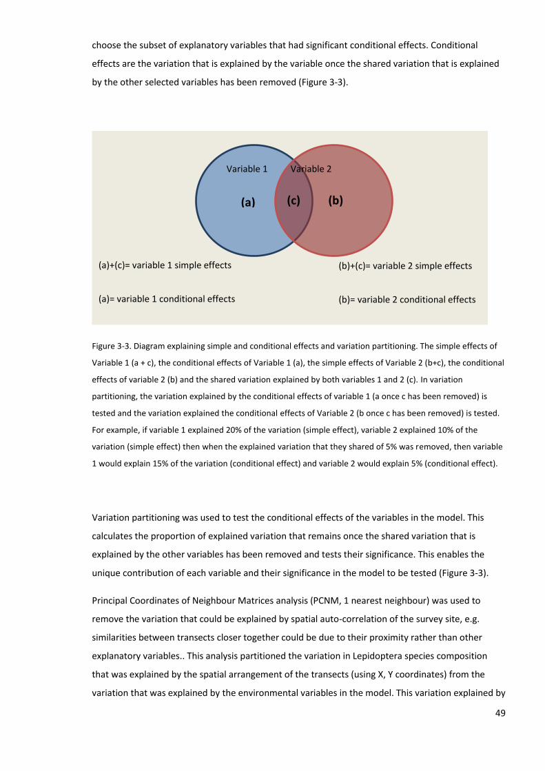
49
choose the subset of explanatory variables that had significant conditional effects. Conditional
effects are the variation that is explained by the variable once the shared variation that is explained
by the other selected variables has been removed (Figure 3-3).
Figure 3-3. Diagram explaining simple and conditional effects and variation partitioning. The simple effects of
Variable 1 (a + c), the conditional effects of Variable 1 (a), the simple effects of Variable 2 (b+c), the conditional
effects of variable 2 (b) and the shared variation explained by both variables 1 and 2 (c). In variation
partitioning, the variation explained by the conditional effects of variable 1 (a once c has been removed) is
tested and the variation explained the conditional effects of Variable 2 (b once c has been removed) is tested.
For example, if variable 1 explained 20% of the variation (simple effect), variable 2 explained 10% of the
variation (simple effect) then when the explained variation that they shared of 5% was removed, then variable
1 would explain 15% of the variation (conditional effect) and variable 2 would explain 5% (conditional effect).
Variation partitioning was used to test the conditional effects of the variables in the model. This
calculates the proportion of explained variation that remains once the shared variation that is
explained by the other variables has been removed and tests their significance. This enables the
unique contribution of each variable and their significance in the model to be tested (Figure 3-3).
Principal Coordinates of Neighbour Matrices analysis (PCNM, 1 nearest neighbour) was used to
remove the variation that could be explained by spatial auto-correlation of the survey site, e.g.
similarities between transects closer together could be due to their proximity rather than other
explanatory variables.. This analysis partitioned the variation in Lepidoptera species composition
that was explained by the spatial arrangement of the transects (using X, Y coordinates) from the
variation that was explained by the environmental variables in the model. This variation explained by
(a) (b) (c)
(a)+(c)= variable 1 simple effects
(a)= variable 1 conditional effects
(b)+(c)= variable 2 simple effects
(b)= variable 2 conditional effects
Variable 1 Variable 2

50
the spatial arrangement was then removed from the model which contains the environmental
variables and the significance of the new model was tested. This works similarly to Variation
Partitioning as illustrated in Figure 3-3 but in this case variable 1 is the set of environmental variables
and variable 2 is the spatial variable. This was done for each model but was not significant in
explaining the variation in Lepidoptera communities and so is not reported in the following results.
Lepidoptera total density, species richness and individual species response to environmental
variables were analysed using Generalized Linear Models (Linear response, Poisson distribution) and
used to select ecologically relevant variables for inclusion in the ordination models (see Appendix B
for all GLM and RDA results). The age of the habitat type was assigned for grassland re-creation
fields as the number of years since sown with species rich grassland seed. Chalk grassland was
assigned an age of 60 years as this is the number of years estimated for some re-creation grasslands
to reach the same botanical conditions as chalk grassland (Fagan et al. 2008) and semi-improved
pasture was assigned an age of three years for. All species and samples were given equal weighting.
Co-variables were also included if they explained a high proportion of the variation but were not of
interest. A co-variable is an explanatory variable that is either a noise or nuisance variable where the
variation that it explains needs to be factored out or a variable that is important but not of interest
to the study questions. Potential co-variables were measures of mean and variation (Coefficient of
Variation) in cloud coverage and wind speed as well as temperature and sampling day. For habitat
transects, no co-variables were used as Lepidoptera community assemblages were not significantly
affected by weather conditions or sampling day (Appendix B). For matrix transects the mean
percentage of cloud cover was used as a co-variable as it had the highest significance and lowest AIC
when explaining Lepidoptera density in GLM and explained 24.1% of variation in community
assemblages (Appendix B).
3.4 Results
3.4.1 Lepidoptera density, species richness and distributions in habitat and matrix transects
For habitat transects, 1,121 individual Lepidoptera were recorded of 18 different butterfly species
and one day-flying moth species (Zygaena filipendulae). Species composition results indicated that
Lepidoptera communities were approaching that of the target habitat. In older grassland re-creation
(7-10 years since sowing) there was a lower Bray-Curtis dissimilarity compared with newer re-
creation (1-5 years since sowing) but this was not significant. This was attributed to the colonisation
of grassland associated butterflies such as the Marbled White (Melanargia galathea), Common Blue
(Polyommatus icarus) and Meadow Brown (Maniola jurtina) (Table 3-2,Table 3-3).

51
Lepidoptera species more associated with short-grass and herb-rich habitats (Shreeve et al. 2001)
which are characteristic of calcareous grassland such as Adonis Blue (Lysandra bellargus) and Brown
Argus (Arica agestis see Appendix B), were restricted to chalk grassland fragments and absent from
the grassland re-creation. Species associated with ruderal-vegetation and of widespread mobility
such as the Small Tortoiseshell (Aglais urticae) and Large White (Pieris brassicae) were surveyed in
chalk grassland fragments, grassland re-creation fields and arable land (see Appendix B for
Lepidoptera distribution in semi-improved pasture and arable land).
Table 3-2. The eight focal species recorded at surveys at the Stonehenge landscape including code used for
figures and graphs in this chapter. Ecological group of species associated with Ruderal vegetation (ruderal-
veg), short-turf herb rich grassland (herb-rich) and short-tall sward open grassland (open-grass) (Shreeve et al.
2001) and mobility groups of sedentary, intermediate and widespread (Pollard & Yates 1993).
Common name Latin name Code Ecological
group
Mobility
group
Adonis Blue Lysandra bellargus Lys.bel Herb-rich Sedentary
Small Heath Coenonympha pamphilus Coe.pam Open-grass Sedentary
Marbled White Melanargia galathea Mel.gal Open-grass Sedentary
6-spot Burnet Zygaena filipendulae Zyg.fil Herb-rich Sedentary
Common Blue Polyommatus icarus Pol.ica Herb-rich Intermediate
Meadow Brown Maniola jurtina Man.jur Open-grass Sedentary
Small Tortoiseshell Aglais urticae Agl.urt Ruderal-veg Widespread
Large White Pieris brassicae Pie.bra Ruderal-veg Widespread

52
Table 3-3. The mean Bray-Curtis dissimilarity and 1 Standard Error (SE) of Lepidoptera communities between
the highest quality chalk grassland fragment reference habitat patch (Luxenborough Bank) and the other land
cover types. The total number of eight focal Lepidoptera species surveyed in different land-cover types of
chalk grassland fragments (Chalk), barrow groups (Barrow), older grassland re-creation fields 7−10 years old
(Older grass) and newer grassland re-creation fields 1−5 years old (Newer grass). The mean and 1 Standard
Error of Lepidoptera individuals surveyed in transects extending from chalk grassland fragments into a matrix
type of either newer grassland re-creation of 1-2 years old (Newer grass) or Arable land (Arable).
Habitat transects Matrix transects
Chalk Barrow Older grass Newer grass Newer Grass Arable
Bray-Curtis dissimilarity 0.33 0.39 0.48 0.58 N/A N/A
SE 0.03 0.09 0.09 0.05 N/A N/A
Lysandra bellargus 1.334 2.00 0.50
SE 0.88 2.00 0.29
Coenonympha pamphilus 0.67 3.00 1.50
SE 0.67 2.52 1.50
Melanargia galathea 0.67 4.00 0.33 2.50
SE 0.33 3.06 0.33 0.87
Zygaena filipendulae 22.33 0.33 54.00 0.33 0.75
SE 16.70 0.33 45.71 0.33 0.48
Polyommatus icarus 12.67 30.00 9.67 2.33 20.50
SE 2.85 25.51 4.48 1.86 10.37
Maniola jurtina 33.67 34.33 16.67 1.33 10.75 5.75
SE 29.20 16.37 8.01 0.88 4.37 0.85
Aglais urticae 6.33 9.67 5.75 2.50
SE 3.38 9.67 3.33 0.87
Pieris brassicae 30.33 34.33 8.00 5.33 5.25 6.50
SE 18.66 17.02 5.69 2.03 1.49 2.63
There were higher, but not statistically significant Lepidoptera densities in chalk grassland reference
habitat patches on slopes and Barrow groups compared to grassland re-creation fields of all ages
(Wilcoxon test, W=30, p=0.0649 per 100 m of habitat transect). Out of all the grassland re-creation

53
fields, Seven Barrows and Noice's Piece (sown in 2000 and 2003, respectively) had the highest
densities indicating that they were approaching the conditions of the reference habitat. There was
significantly higher Lepidoptera richness at target chalk grassland habitat patches compared to
grassland re-creation habitat patches (Wilcoxon test, W=36, p=0.0022), but no significant difference
in densities of different Lepidoptera ecological and mobility groups (p>0.05, Appendix B for full
results and mixed-effect models) (Table 3.3, Figure 3-4).
For matrix transects surveys crossing from target chalk grassland fragments into adjacent matrix
types, 582 individual Lepidoptera were recorded consisting of 16 butterfly species and three day-
flying moth species; the 6-spot Burnet moth (Zygaena filipendulae), Forester moth (Adscita statices
or possibly Cistus Forester Adscita geryon) and Hummingbird Hawk moth (Macroglossum
stellatarum). There were no significant differences between mean densities of Lepidoptera, species
richness or densities of the different ecological groups along transects from chalk grassland
fragments into newer grassland re-creation of 1-2 years old compared to arable land mixed-effects
models (p>0.05, Appendix B) .This result remained even when only Lepidoptera surveyed in the
matrix part of the transect were used in the analysis (results not shown).
Figure 3-4. The, a) total Lepidoptera density (Wilcoxon sum rank test, W=30 p=0.0649) and, b) species richness
(Wilcoxon sum rank test, W=36, p=0.0004) in broad habitat types of chalk grassland on slopes and barrows and
grassland re-creation ages 1-10 years since sowing with regional seed mixtures. Significance p<0.001 ***.
Chalk grassland fragments (on slopes and barrows) had significantly higher mean densities of nectar
flowers in the Asteraceae family and borderline significantly higher nectar flower richness (W=31,
p=0.0411 and W=30, p=0.0649, respectively) and borderline significantly lower mean densities of
Fabaceae nectar flowers (W=5.5, p=0.0542). Other variables were not significant (p>0.05) (see
Appendix B for statistical comparison between all environmental variables).
0
5
10
15
20
25
30
35
Total density
Lep
ido
pte
ra d
en
sity
pe
r 1
00
m
(me
an)
0
1
2
3
4
5
6
7
Species Richness
Lep
ido
pte
ra s
pe
cie
s ri
chn
ess
p
er
10
0m
(m
ean
)
Chalk fragments and barrow
Grassland re-creation 1-10 years old
***
a b

54
A total of 234 Lepidoptera were recorded feeding on nectar plants in habitat transects. The nectar
feeding interactions in the grassland re-creation were less diverse and dominated by a few individual
species compared to the more complex interactions in the chalk grassland fragments, which also had
the highest density of Lepidoptera feeding, followed by the barrow groups (Appendix B). The species
that dominated the Lepidoptera-nectar plant interaction network were 6-spot Burnet moth
(Zygaena filipendulae) and Meadow Brown (Maniola jurtina) and Geer Knapweed (Centaurea
scabiosa), Creeping Thistle (Cirsium arvense) and Common Knapweed (Centaurea nigra) nectar
plants.
3.4.2 Community compositions
3.4.2.1 Model, a) measures of habitat quality
(i) Habitat transects
Unconstrained PCA ordination on habitat transects showed that axes 1 and 2 explained 74.5% of the
variation, which suggested strong gradients in the data. Transects in semi-improved pasture, arable
land and new grassland re-creation (1-3 years old) were clustered to the mid left of the sample plot
and grassland re-creation fields sown in the year 2000 and 2003 (h and j) were more similar to chalk
grassland fragments on slopes (a and b) than to the other grassland re-creation fields as these were
clustered close together(Figure 3-5. a).
The percentage coverage of linear features within a 100 m buffer of transects was selected for the
habitat quality model as this variable had six significant species responses including Maniola jurtina,
Melanargia galathea, Pieris brassicae, Pieris napi, Polyommatus icarus and Zygaena filipendulae
(GLM positive linear response) compared to five at the 250 m scale (all species listed previously
except Melanargia galathea) and was therefore used in the habitat transect model below (see
Appendix B for all landscape RDA results).
In a constrained RDA, the environmental variables of mean coverage of bare ground, vegetation
density, nectar flower richness, the age of the habitat (how many years it takes to restore) and
percentage coverage of natural linear features within the 100 m buffer (all variables had a positive
correlation) explained 63.8% (47.3% adjusted) of the variation (first axis p=0.004, all axes p=0.002).
After interactive forward selection, the age, nectar richness and vegetation density were retained in
the model and explained 55.1% (44.7% adjusted) of the variation (first and all axes p=0.002) (Figure
3-5, b, Table 3-4).
Age and vegetation density had significant conditional effects and a positive correlation once the
shared variation had been removed from variation partitioning (p=0.035, 0.019, respectively). When
constrained by ecological and then mobility group this model was borderline significant and

55
significant, respectively (first axis p=0.056, all axes p=0.114 for ecology group and first axis p=0.024,
all axes p=0.028 for mobility group).
Figure 3-5. a) Principal Component Analysis, axis 1 and 2 explained 74.5% cumulatively of the variation for
habitat transects. a-m relate to habitat patches/fields in Table 3-1 (note d not surveyed in habitat transects). b)
Redundancy Analysis model (ai) of habitat quality in habitat transects explained 55.1% of the variation, axis 1
and 2 explained 50.34% of this cumulatively (first and all axes p=0.002). The ecological group of the
Lepidoptera species response is illustrated by the colour of the arrows on, b) of ruderal-veg (dark blue), open-
grass (pale blue), herb-rich (red) and woodland (orange).For non focal species abbreviations see Appendix B.
a b axis 1 55.4%
axis
2 1
9.2
%
axis 1 43.2%
axis
2 7
.1%

56
Figure 3-6. a) Redundancy Analysis model constrained by matrix type of arable or grassland re-creation
explained 33.3% of the variation (all axes p=0.004), axis 1 and 2 explained 61.8% of this cumulatively. b)
Redundancy Analysis model (aii) of habitat quality in matrix transects using the mean cloud coverage as a co-
variable explained 39.6% of the variation (first axis p= 0.014, all axes p=0.004), axis 1 and 2 explained 39.9% of
this cumulatively. Environmental variables (black arrows) were the age to re-create that habitat (Age2), nectar
flower species richness (NectarRc) and vegetation density (VegM). The ecological group of the Lepidoptera
species response illustrated by colour of arrows on, b) and, d) of ruderal-veg (dark blue), open-grass (pale
blue), herb-rich (red) and Woodland (orange). For non focal species abbreviations see Appendix B.
(ii) Matrix transects
Unconstrained PCA ordination of matrix transects showed that axis 1 and 2 explained 6.9% of the
variation cumulatively, suggesting that there were strong trends in the data. An RDA constrained by
matrix type of arable or new grassland re-creation explained 33.3% (26.60% adjusted) of the
variation (all axes p=0.004) (Figure 3-6, a, Table 3-4).
An RDA model using the mean percentage of cloud coverage as a co-variable and mean vegetation
density, bare ground percentage coverage and nectar flower richness (all had negative correlations
except nectar flower richness) as explanatory variables explained 51.6% (30.9% adjusted) of
variation (first axis p=0.016, all axes p=0.002). Mean vegetation density and nectar flower richness
were retained in the model after interactive forward selection resulting in a model that explained
39.6% (24.9% adjusted) of the variation (first axis p= 0.014, all axes p=0.004, Figure 3-6, b, Table 3-4).
The mean vegetation density and percentage coverage of cloud had significant conditional effects
(negative correlation) when the shared variation was removed from variation partitioning (p=0.010
a b axis 1 33.3%
axis
2 2
8.5
%
axis 1 27.6%
axis
2 1
2. 3
%

57
and p=0.066, respectively). When constrained by ecological and then mobility group the model was
significant and not significant, respectively (first axis p=0.030, all axes p=0.002 and first axis p=0.280,
all axes p=0.290).
Table 3-4. Summary of unconstrained (Principal Coordinate Analysis) and constrained (Redundancy Analysis)
models including the full model containing all the environmental variables (Full) and after interactive forward
selection (FS=) and the total (Total) and adjusted (Adj) variation explained. The cumulative explained variation
of the first four axes (axis1-axis4) and the p value of the first and all axes from the Monte-Carlo permutation
test. Whether the model was significant when constrained by ecological or mobility group (first axis p and all
axes p=). Environmental variables include Age of the habitat (Age2), proportion of linear features in a 100m
buffer (Lin100), Nectar flower species richness (NectarRc), mean percentage coverage of bare ground (BG%M),
mean vegetation density (VegM) and mean percentage cloud coverage (CloudM).
Variation
explained %
Explained variation (cumulative) Permutation
test p=
Model type Total Adj Axis1 Axis2 Axis3 Axis4 First All
Unconstrained models
Unconstrained (habitat transect) 55.35 74.54 85.68 92.68
Unconstrained (matrix transect) 38.45 64.89 77.94 84.01
Matrix type (Arable and newer re-
creation grassland)
33.30 26.60 33.29 61.75 74.91 82.20 0.004
a) Habitat quality
i) habitat transects
Age2, Lin100, BG%M, NectarRc,
VegM
63.80 47.30 45.93 53.28 60.39 63.46 0.004 0.002
FS=Age 2, VegM, NectarRc 55.10 44.70 43.23 50.34 55.06 73.08 0.002 0.002
Ecological group 24.40 9.30 23.82 24.39 24.40 67.55 0.064 0.138
Mobility group 19.70 9.70 19.43 19.71 67.91 86.44 0.058 0.096
ii) matrix transects
(CloudM), VegM, BG%M, NectarRc 51.60 30.90 28.98 42.6 51.62 69.37 0.016 0.002
FS=(CoudM), VegM, NectarRc 39.90 24.90 27.62 39.89 59.35 73.62 0.014 0.004
Ecological group 41.70 29.20 25.09 39.31 41.68 76.40 0.030 0.002
Mobility group 15.00 3.60 12.17 14.96 53.16 84.76 0.280 0.290

58
b) Nectar resources
i) habitat transects
NectarM, NectarRc, AstM, DipM,
FabM
56.20 36.30 35.36 49.99 55.28 56.02 0.052 0.004
FS=NectarRc and DipM 42.70 34.50 32.99 42.66 69.97 82.41 0.004 0.002
Ecological group 37.40 24.80 24.28 37.36 80.24 100.00 0.082 0.024
Mobility group 24.30 14.80 23.96 24.26 69.87 100.00 0.038 0.064
ii) matrix transects
NectarRc, AstM, DipM, FabM 62.70 41.40 34.53 53.51 60.65 62.73 0.008 0.002
FS= NectarRc, AstM 50.10 39.00 34.39 50.06 65.44 78.65 0.002 0.002
Ecological group 29.60 14.50 25.97 29.55 80.62 100.00 0.064 0.082
Mobility group 17.50 6.50 14.56 17.5 69.23 100.00 0.250 0.220
c) Vegetation characteristics
i) habitat transects
VegM, VegTranCV, VegSegCV,
BG%M, BG%TranCV, BG%SegCV
57.40 31.80 40.85 53.93 56.14 57.02 0.028 0.028
FS= VegM, VegTranCV,
BG%TranCV
52.40 41.40 39.03 51.20 52.40 71.80 0.002 0.002
Ecological group 12.00 0.00 9.78 11.18 12.04 63.55 0.666 0.702
Mobility group 4.70 0.00 4.02 4.72 63.30 96.49 0.830 0.838
ii) (matrix transects
BG%M, VegM, BG%TranCV,
VegTranCV
59.20 35.90 35.36 46.86 57.19 59.2 0.01 0.008
FS= BG%M, VegM 41.20 28.10 33.01 41.19 70.39 78.27 0.004 0.002
Ecological group 21.00 4.10 19.42 21.00 77.47 100.00 0.286 0.356
Mobility group 11.00 0.00 10.70 10.99 72.14 100.00 0.418 0.458

59
3.4.2.2 Model, b) measures of nectar resource
(i) Habitat transects
Nectar flower richness and the mean density of Asteraceae, Fabaceae and Dipsacaceae flowers (all
positive correlation) explained 56.2% (36.3% adjusted) of the variation in RDA (first axis p=0.052, all
axes p=0.004). Nectar flower richness and the mean density of Dipsacaceae flowers were retained in
the model after interactive forward selection and explained 42.7% (34.5% adjusted) of the variation
(first axis p=0.004, all axes p=0.002) (Figure 3-7, a, Table 3-4).
Nectar flower richness and the mean density of Dipsacaceae flowers had significant conditional
effects and positive correlation once the shared effect had been removed from variation partitioning
(p=0.017, 0.015, respectively). Variation partitioning of the three nectar plant families showed that
Dipsacaceae had significant conditional effects and Fabaceae and Asteraceae did not once the
shared variation was taken out (p=0.018, 0.094 and 0.131, respectively). When constrained by
ecological and then mobility groups, the model was borderline significant and significant,
respectively (first axis p=0.082, all axes p=0.038 and first axis p=0.024, all axes p=0.064).

60
Figure 3-7. a) Redundancy Analysis model (bi) of nectar resources in habitat transects explained 42.7% of the
variation (first axis p=0.004, all axes p=0.002), axis 1 and 2 explained 42.7% of this cumulatively. b)
Redundancy Analysis model (bii) of nectar resources in matrix transects explained 50.1% of the variation (first
axis p=0.002, all axes p=0.002), axis 1 and 2 explained 50.1% of this cumulatively. Ecological group of the
Lepidoptera species response illustrated by the colour of the arrows of ruderal-veg (dark blue), Open-grass
(pale blue), Herb-rich (red) and Woodland (orange). For non focal species abbreviations see Appendix B
Figure 3-8. (a) Redundancy Analysis model (ci) of vegetation characteristics in habitat transects explained
52.40% of variation (first and all axes p=0.002), axis 1 and 2 explained 51.2% cumulatively. (b) Redundancy
Analysis model (cii) of vegetation characteristics in matrix transects explained 41.2% of the variation (first axis
p=0.004, all axes p=0.002), Axis 1 and 2 explain 41.2% cumulatively. Environmental variables (black arrows)
were nectar flower species richness (NectarRc), mean density of Dipsacaceae flowers (DipM), mean density of
Asteraceae flowers (AstM), mean vegetation density (VegM) and the within transect variation of vegetation
density (VegTranCV) and bare ground percentage coverage (BG%TranCV). Ecological group of the Lepidoptera
species response is illustrated by the colour of the arrows of ruderal-veg (dark blue), Open-grass (pale blue),
Herb-rich (red) and Woodland (orange). For non focal species abbreviations see Appendix B
a b
a b
axis 1 33.0%
axis
2 9
.7%
axis 1 34.4%
axis
2 1
6.2
%
axis 1 39.03%
axis
2 1
.2%
axis 1 33.0%
axis
2 8
.2%

61
(ii) Matrix transects
Nectar flower richness and the mean densities of Asteraceae, Dipsacaceae and Fabaceae nectar
plant families (all positive correlation) explained 62.7% (41.4% adjusted) of the variation in RDA (first
axis p=0.008, all axes p=0.002). After interactive forward selection the mean nectar flower richness
and the mean number of Asteraceae flowers were retained in the model, explaining 50.1% (39.0%
adjusted) of variation (first axis p=0.002, all axes p=0.002) (Figure 3-7, b, Table 3-4).
The mean number of Asteraceae flowers and nectar flower species richness had significant
conditional effects and positive correlation once the shared variation had been removed from
variation partitioning (p=0.006 and 0.008, respectively). Variation partitioning of the three nectar
flower families showed that only Asteraceae had significant conditional effects (p=0.044). When
constrained by ecological and then mobility group the nectar resource models were not significant.
3.4.2.3 Model, c) vegetation characteristics models
(i) Habitat transect
Vegetation characteristics of vegetation density and bare ground percentage coverage mean and
within transect and within segment variation (all positive correlation) explained 57.4% (31.8%
adjusted) of variation in RDA (first and all axes p=0.028). Vegetation density and bare ground within
transect variation and mean vegetation density were retained after interactive forward selection
and explained 52.4% (41.40% adjusted) of variation (first and all axes p=0.002) (Figure 3-8, a, Table
3-4).
Mean vegetation density and variation in the percentage coverage of bare ground had significant
conditional effects and negative correlations after the shared variation had been removed from
variation partitioning (p=0.004 and 0.014, respectively). The model was not significant when
constrained by ecological or mobility group.
(ii) Matrix transects
The mean percentage coverage of bare ground and vegetation density (negative correlation)and the
within transect variation of bare ground coverage and vegetation density (positive correlation)
explained 59.2% (35.9% adjusted) of the variation (RDA, first axis p=0.01, all axes p=0.008). The
mean bare ground coverage and vegetation density were retained in the model after interactive
forward selection resulted in a model explaining 41.2% (28.1% adjusted) of the variation (RDA, first
axis p=0.004, all axes p=0.002) (Figure 3-8, b Table 3-4).

62
Vegetation density had significant conditional effects once the shared variation had been removed
from variation partitioning (p=0.014). The model was not significant when constrained by ecological
or mobility group.
3.4.2.4 Individual species response to the environmental variables
There were species-specific responses to the environmental variables, with all focal species
associated with the increasing age of the habitat except the 6-spot Burnet moth (Zygaena
filipendulae), whose response was explained significantly better by a quadratic function. All focal
species were associated with increases in nectar flower richness except for Small Tortoiseshell
(Aglais urticae) and the 6-spot Burnet moth (Zygaena filipendulae) in habitat transects and all except
Adonis Blue (Lysandra bellargus) and Large White (Pieris brassicae) in matrix transects. The species
most associated with increased nectar flower families were Aglais urticae, Lysandra bellargus,
Meadow Brown (Maniola jurtina), Pieris brassicae and Common Blue (Polyommatus icarus) to
Dipsacaceae and Aglais urticae, Maniola jurtina, Pieris brassicae and Zygaena filipendulae to
Asteraceae (Table 3-5).
All focal species were significantly positively associated with measures of increased vegetation
density in habitat transects except Lysandra bellargus and Small Heath (Coenonympha pamphilus)
(although these two species had low densities so may have not been sufficient to fit a GLM). For
matrix transects, Lysandra bellargus and Pieris brassicae did not have a significant response to
vegetation density but the other six focal species had significant responses but differed in their
positive or negative correlations to this environmental variable (Table 3-5).
In habitat transects all of the significant environmental variables in the final models had a positive
correlation with butterfly response, however, in the matrix transects these variables had a negative
correlation. These include the density of Asteraceae flowers for Zygaena filipendulae, the
percentage coverage of bare ground for Aglais urticae, Maniola jurtina and Polyommatus icarus, the
richness of nectar flowers for Melanargia galathea and Zygaena filipendulae and mean vegetation
density for all but Melanargia galathea (positive correlation) and Lysandra bellargus and Maniola
jurtina (no effect).

63
Table 3-5. Individual species response to the significant environmental variables in habitat transects of age of
habitat (Age2), mean density of Dipsacaceae flowers (DipM), mean vegetation density (in cm, VegM) and the
within transect coefficient of variation of vegetation density (VegTranCV) and percentage coverage of bare
ground (BG%TranCV). Individual species response to the significant environmental variables in matrix transects
of mean density of Asteraceae flowers (AstM), percentage coverage of bare ground (BG%M), nectar flower
richness (NectarRc), mean vegetation density (cm) (VegM) and percentage cloud coverage (CloudM used as a
covariable in RDA analysis). R2(%) of linear GLM (Poisson distribution, log-link function, only significant R
2
shown) and p value Significance p<0.001 ***, p<0.01 **, p<0.05 *, 0.1<p>0.05 (*). Direction of linear response
either positive (+) or negative correlation (-). For individual species response to all environmental variables see
Appendix B.
Variable
Ag
lais
urt
ica
e
Co
eno
nym
ph
a p
am
ph
ilus
Lysa
nd
ra b
ella
rgu
s
Ma
nio
la ju
rtin
a
Mel
an
arg
ia g
ala
thea
Pie
ris
bra
ssic
ae
Po
lyo
mm
atu
s ic
aru
s
Zyg
aen
a f
ilip
end
ula
e
Habitat transects
Age2 R2 48.40(+) (+) 52.90(+) 45.60(+) (+) 50.60(+) 42.70(+)
p= ** (*) * *** (*) *** ***
BG%TanCV R2 40.30(+) 16.30(+) 38.30(+)
p= *** ** ***
DipM R2 43.60(+) 15.20(+) 8.50(+) 17.10(+)
p= * ** * **
NectarRc R2 (+) 63.00(+) 36.10(+) (+) 17.60(+) 71.40(+)
p= (*) * *** (*) ** ***
VegM R2 (+) 79.90(+) (+) 48.20(+) 38.70(+) 11.10(+)
p= (*) *** (*) *** *** **
VegTranCV R2 47.50(+) 52.2(+) 44.90(+) 30.40(+)
p= *** * *** ***
Matrix transects
AstM R2 81.70(+) 36.30(+) 48.50(+) 43.40(-)
p= *** ** ** **
BG%M R2 30.10(-) 20.40(-) 35.50(+) 19.60(-)

64
p= ** * * ***
CloudM R2 62.50(-) 50.70(-) 18.80(-) 32.80(-) 7.70(-)
p= *** ** ***
NectarRc R2 27.60(+) 100.00(+) 26.50(+) 28.70(-) 29.70(+) 39.30(-)
p= ** * * * *** **
VegM R2 14.90(-) 28.80(-) 47.00(+) 70.00(-) 12.50(+)
p= * * ** ** *
3.5 Discussion
3.5.1 Biodiversity enhancement as a result of the grassland re-creation at the landscape scale for
Lepidoptera
3.5.1.1 Lepidoptera density, richness and community compositions
There was evidence of biodiversity enhancement within the relatively short time period of under a
decade in terms of Lepidoptera density, richness and community compositions in response to the
grassland re-creation in the Stonehenge landscape. There was a borderline significant difference
between the density of Lepidoptera in the grassland re-creation compared to chalk grassland
fragments. There were increases in community similarity (Bray-Curtis index) and older grassland re-
creation sown in 2000 and 2003 were more similar to chalk grassland fragments on slopes than to
the other grassland re-creation fields (multivariate analysis).
Previous surveys of the botanical characteristics of this grassland restoration and re-creation project
have shown that the re-creation fields have approached similar ecological conditions to the donor
habitat patches within 7-10 years (Campbell 2009; Pemberton 2011; Twiston-Davies et al. in press)
and other calcareous grassland studies (Piqueray et al. 2011; Prach et al. 2013), supporting these
results for relatively rapid colonisation. Invertebrates are likely to lag behind botanical colonisation
and are expected within 10 years for butterfly communities (Woodcock et al. 2012a), although
invertebrates characteristic of the target habitat can colonise new grasslands in as little as 2 years
and some generalist species colonise newly restored habitats at the early stages (Deri et al. 2011).
Biodiversity enhancement is limited by low Lepidoptera species richness in grassland re-creation and
the community compositions of newer grassland re-creation. Grassland re-creation overall had
significantly lower species richness compared to chalk grassland fragments and a matrix of newer
grassland re-creation 1-2 years old adjacent to chalk grassland fragments was not significantly
different in Lepidoptera density or species richness compared to arable land. Newer grassland re-

65
creation was more similar in terms of community compositions to semi-improved pasture and arable
land in multivariate analysis.
Results from the nectar feeding interactions showed differences between chalk fragments and older
and newer grassland re-creation with less diverse networks that were dominated by some individual
species in grassland re-creation habitat patches (Appendix B).
3.5.1.2 Species specific response
Many Lepidoptera species surveyed across the Stonehenge Landscape were characteristic of
calcareous grasslands in Europe, including the Brown Argus (Arica agestis), Coenonympha
pamphilus, Small Copper (Lycaena phlaeas), Marbled White (Melenargia galathea), Polyommatus
icarus and Lysandra bellargus (van Swaay 2002). Some of these species, such as Coenonympha
pamphilus and Melanargia galathea, are more associated with open-grass and mesotrophic
conditions in the UK (Shreeve et al. 2001).
The response of Lepidoptera to the significant environmental variables in terms of fit, direction and
function was species specific and their distributions across the habitats of the Stonehenge Landscape
were most likely attributed to their larval host specificity and the presence of these plants in the
grassland re-creation fields. The colonisation of the less specialist species such as Zygaena
filipendulae and Melanargia galathea in the older grassland re-creation fields is likely due to the
establishment of their larval host plants (Lotus corniculatus and Festuca sp. respectively, Campbell
2009; Pemberton 2011). These species also have weaker associations with short-turf, herb-rich
grassland habitats which are characteristics associated with chalk grassland (Shreeve et al. 2001; van
Swaay 2002) and therefore further expansion of these Lepidoptera species into younger grassland
re-creation fields would be predicted in the future.
Lysandra bellargus did not have a significant linear relationship with nectar flower species richness
and this is more likely due to its overall low numbers in matrix transects rather than a changed
association with nectar flower richness in the matrix compared to the habitat.
The more specialist species such as Lysandra bellargus, associated with chalk grassland and short-
turf, herb rich habitats were absent from grassland re-creation fields (Shreeve et al. 2001; van Swaay
2002). This is probably due to the restriction of their larval host plant Horseshoe Vetch (Hippocrepis
comosa) to chalk grassland fragments, potentially inhibiting colonisation (although this species was
in the original seed mixture sown into the 2000 grassland re-creation field) and Lysandra bellargus
adults and eggs have been surveyed on Hippocrepis comosa on these fragments (Appendix B).
Individuals of Lysandra bellargus were recorded twice in matrix transects of newer grassland re-
creation under 40 m from the chalk grassland fragment, indicating the potential of this new
grassland habitat for additional nectar resources. Additionally, there were plans to extend the

66
grassland re-creation to encompass the chalk grassland fragments on slopes at Full-moon Bank and
Luxenborough Bank which went ahead at the end of the year 2012. The restriction of Lysandra
bellargus to chalk grassland fragments may also be due to their symbiotic relationship with ants
(Myrmica sabuleti and Lasius alienus Forster, Thomas 1983) which may need to colonise these new
habitats along with Lysandra bellargus in order to achieve for biodiversity enhancement for these
species.
3.5.1.3 Summary
It is vital to evaluate grassland re-creation and biodiversity enhancement using a variety of measures
such as Lepidoptera density, richness, the distributions of individual Lepidoptera species and the
community compositions as made evident by differences in these measures of biodiversity
enhancement in this study. Biodiversity enhancement measured on Lepidoptera densities or
richness alone may be inaccurate as communities may be different, for example in a previous study,
d higher densities of Lepidoptera surveyed in sown wildflower meadow strips and no differences
between species richness but the community compositions were however, different (Haaland &
Bersier 2011). The Lepidoptera species specific responses indicate that grassland re-creation may
only result in biodiversity enhancement for some species; whether this relates to different ecological
classifications or mobility groups is discussed (section 3.5.3). Biodiversity enhancement should also
be measured in terms of ecological interactions and a pilot study to investigate Lepidoptera nectar
feeding was conducted in the different habitats types of Lepidoptera feeding on nectar plants
(Appendix B).
3.5.2 The habitat and landscape traits that encourage colonisation of new habitats and the
movement of species from isolated chalk grassland fragments
3.5.2.1 Habitat scale environmental variables
The age of the habitat (or age to re-create that habitat) explained a large proportion of the variation
in the multivariate analyses for habitat transects, significantly explaining Lepidoptera density and
richness in GLMs (Appendix B), Lepidoptera occurrence in the RDA analysis and had significant
conditional effects (along with vegetation density) after variation partitioning.
Multivariate analysis results indicated the importance of environmental variables that could be
managed for, such as increased nectar flower richness and variation in vegetation density for
Lepidoptera occurrence. Vegetation density, nectar flower richness and nectar flowers in the
Dipsacaceae and Asteraceae families were the environmental variables significantly explaining
Lepidoptera occurrence for both habitat and matrix type transects. Although these environmental
variables were positively correlated with the age of the habitat (correlation coefficient of 0.51 for
vegetation density and 0.69 for nectar flower richness in habitat transects, (data not shown),

67
vegetation density explained more variation than the age of the habitat and was also significant
after variation partitioning. Nectar flower richness was not significant after variation partitioning but
was significantly positively correlated with Lepidoptera density and richness whereas vegetation
density was only significant for density (richness was borderline significant) in habitat type GLMs
(Appendix B). In addition to this, the effect of increasing vegetation density in matrix transects was
significantly negative.
Nectar source abundance and diversity are important variables in explaining Lepidoptera occurrence
(Clausen et al. 2001; Haaland & Bersier 2011) and flower visitor diversity (Ebeling et al. 2008),
although does not necessarily reflect pollinator diversity (King et al. 2013). The abundance of nectar
rich sources in composite flowers such as Field Scabious (Knautia arvensis) in the Dipsacaceae family
for example were the preferred nectar plant in uncultivated habitats of organic farms for butterflies
and burnet moths (Clausen et al. 2001).
Responses to the environmental variables were species specific but species within the same
ecological and mobility groups responded similarly. All species that had a significant response to
increased nectar flower richness and densities of nectar flowers in the Dipsacaceae family had a
positive correlation with these variables. Lepidoptera individual species response was more variable
for in terms of significance and direction in response to increased vegetation density.
Botanically, differences between chalk grassland fragments habitat patches and grassland re-
creation fields of all ages were significant in terms of nectar plant richness and the densities of
Asteraceae and Fabaceae families (Appendix B). In chalk grassland fragment reference habitat
patches there were significantly higher mean densities of nectar flowers in the Asteraceae family
(dominated by knapweeds such as Common Knapweed, Centaurea nigra as well as Smooth
Hawksbeard, Crepis capillaris), borderline significantly higher nectar flower richness and significantly
lower mean densities of Fabaceae (dominated by Sainfoin, Onobrychis viciifolia and Bird's-foot
Trefoil, Lotus corniculatus). These differences in nectar resources between grassland re-creation and
reference habitat patches were significant in explaining Lepidoptera community compositions and
the responses of individual species (RDA, GLM).
3.5.2.2 The influence of the landscape
The results presented suggest that linear features were not as important for Lepidoptera occurrence
as habitat characteristics in this study as they were not retained in habitat type models after
interactive forward selection. These findings are supported by some previous studies that concluded
that habitat patch quality is more important for overall species conservation actions and for
butterflies in calcareous grasslands and (Hodgson et al. 2011; Hodgson et al. 2009; Rosin et al. 2012).
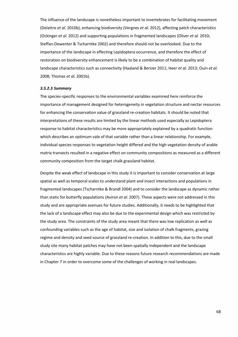
68
The influence of the landscape is nonetheless important to invertebrates for facilitating movement
(Delattre et al. 2010b), enhancing biodiversity (Vergnes et al. 2012), affecting patch characteristics
(Ockinger et al. 2012) and supporting populations in fragmented landscapes (Oliver et al. 2010;
Steffan-Dewenter & Tscharntke 2002) and therefore should not be overlooked. Due to the
importance of the landscape in effecting Lepidoptera occurrence, and therefore the effect of
restoration on biodiversity enhancement is likely to be a combination of habitat quality and
landscape characteristics such as connectivity (Haaland & Bersier 2011; Heer et al. 2013; Ouin et al.
2008; Thomas et al. 2001b).
3.5.2.3 Summary
The species-specific responses to the environmental variables examined here reinforce the
importance of management designed for heterogeneity in vegetation structure and nectar resources
for enhancing the conservation value of grassland re-creation habitats. It should be noted that
interpretations of these results are limited by the linear methods used especially as Lepidoptera
response to habitat characteristics may be more appropriately explained by a quadratic function
which describes an optimum vale of that variable rather than a linear relationship. For example,
individual species responses to vegetation height differed and the high vegetation density of arable
matrix transects resulted in a negative effect on community compositions as measured as a different
community composition from the target chalk grassland habitat.
Despite the weak effect of landscape in this study it is important to consider conservation at large
spatial as well as temporal scales to understand plant and insect interactions and populations in
fragmented landscapes (Tscharntke & Brandl 2004) and to consider the landscape as dynamic rather
than static for butterfly populations (Aviron et al. 2007). These aspects were not addressed in this
study and are appropriate avenues for future studies. Additionally, it needs to be highlighted that
the lack of a landscape effect may also be due to the experimental design which was restricted by
the study area. The constraints of the study area meant that there was low replication as well as
confounding variables such as the age of habitat, size and isolation of chalk fragments, grazing
regime and density and seed source of grassland re-creation. In addition to this, due to the small
study site many habitat patches may have not been spatially independent and the landscape
characteristics are highly variable. Due to these reasons future research recommendations are made
in Chapter 7 in order to overcome some of the challenges of working in real landscapes.

69
3.5.3 The species traits that encourage the colonisation of new habitats and the movement from
isolated chalk grassland fragments
3.5.3.1 Ecological group
Open-grass associated species responded positively to grassland re-creation with high abundances
of Maniola jurtina and Melanargia galathea in grassland re-creation fields of all ages. Herb-rich
associated species colonised older grassland re-creation fields; especially Polyommatus icarus and
Zygaena filipendulae. New grassland re-creation potentially encouraged the colonisation of some
herb-rich species as illustrated by the matrix transect results, potentially due to high nectar plant
abundance.
Models were significant (and borderline significant) when constrained by ecological group in cases
when they included environmental variables relating to nectar resources. When the models were
constrained by ecological group they were borderline significant for the habitat quality and nectar
resource models in habitat transects (Table 3-4), significant for the habitat quality in matrix transects
and borderline significant for nectar resources in matrix transects.
3.5.3.2 Mobility group
Lepidoptera species of sedentary, intermediate and widespread mobility were surveyed in grassland
re-creation fields although the species restricted to chalk grassland and barrows in habitat transects
Lysandra bellargus and Coenonympha pamphilus were mainly sedentary. There were no significant
differences between chalk grassland fragments and grassland re-creation fields or between matrixes
of arable or new grassland re-creation in species density due to the species specific responses to
these habitat and matrix types. For example Zygaena filipendulae and Melanargia galathea are
classified as sedentary and were recorded in older restoration and arable matrix types.
Models constrained by mobility group were borderline significant for habitat transects in terms of
the habitat quality and nectar resources. Models constrained by mobility group were also borderline
significant for matrix transects in terms of nectar resources depending on the mobility classification
of the Green-veined/Small White (Pieris napi/Pieris rapae) combined group (was borderline
significant when Pieris napi/Pieris rapae were classed as widespread and reported in the Appendix
B).
3.5.3.3 Summary
It is crucial to consider different ecological and mobility groups of Lepidoptera as these can be
responsible for changes in community compositions due to trait specific responses to habitat and
landscape characteristics (Ockinger et al. 2009; Thomas 2000) and lags in the colonisation times of
particular groups and species (Woodcock et al. 2012a; Woodcock et al. 2012b). Overall, ecological
and mobility groups did not significantly differ between reference and grassland re-creation habitat

70
patches or between arable and new grassland re-creation matrix in terms of mean densities;
however, in multivariate analysis there were significant differences. This was potentially due to
species specific responses as well as high variation between the mean densities of Lepidoptera in
different habitats and the low number of replicate surveys per habitat type. When constrained by
ecological group more models were significant compared to when constrained by mobility group;
however, these groups are not completely independent of one another and the use of these broad
classifications may not remain static as fragmentation-caused selection can alter Lepidoptera traits
and host plant specificity (Hardy et al. 2007; Ockinger & Van Dyck 2012).
3.6 Conclusion
This case study of chalk grassland at the landscape scale in the UK provides evidence that
biodiversity enhancement as a result of grassland re-creation can be obtained within a decade for
some Lepidoptera groups and species. The colonisation of specialist species may lag behind,
requiring additional time and specific habitat management. Habitat conditions that can be managed
for can be as important as the age of the restoration habitat patch and therefore prescribing the
appropriate management is vital to encourage colonisation by a range of groups and species.
Limitations of biodiversity enhancement at this landscape restoration project at the Stonehenge
Landscape arise from the complexity of restoring invertebrate communities. Such restoration
projects will not achieve biodiversity enhancement without the establishment of species specific and
habitat patch characteristic host plants. Insect colonisation will inevitably lag behind vegetation in
restoration projects, but the rate of this can be managed for if the group and species specific
requirements of the target taxa are understood and appropriate management is undertaken.
The main assumption of this study is that butterfly biodiversity as measured by species richness,
abundances and community assemblages can be an indicator for other groups, but this is not always
the case (Biesmeijer et al. 2006; Carvalheiro et al. 2013). Also, this study did not show a landscape
effect on butterfly community assemblages, this may be due to the confounded survey site and low
replication and therefore conclusions relating to landscape effects can not be confidently made
here. This could be addressed in future studies by comparing a number of study landscapes
undergoing restoration. Additionally, species richness and abundances were measured, this is not
always the best measure for biodiversity enhancement and association to a targeted habitat may be
more appropriate, e.g. habitat affinity indices (Deri et al. 2011).
Despite the potential of habitat re-creation to restore connectivity to our fragmented landscapes,
protected areas are still important for biodiversity (Thomas et al. 2012) and this means that habitat

71
re-creation and restoration is just one of a range of methods for landscape conservation and
protection. Overall habitat restoration at the landscape scale is promoted as conservation policy as
an effective method alongside habitat conservation to enhance landscape connectivity, biodiversity
and facilitate the migration of species in response to climate change (Lawton et al. 2010;
Pfadenhauer 2001).

72
Chapter 4 Impacts of habitat creation on boundary-crossing behaviour of
grassland butterflies
4.1 Introduction
Measuring the effect of habitat restoration and re-creation projects on biodiversity is complex (Ruiz-
Jaen & Aide 2005; SER 2004). Just as different taxa respond differently to habitat fragmentation
(Aviron et al. 2005; Diekotter et al. 2008; Hendrickx et al. 2007; Keller et al. 2013; Ricketts 2001),
their response also differs in relation to restoration measures. This means that the effect of
restoration on biodiversity and on the behaviour of organisms may depend on the measures and
identity of species groups studied.
A variety of studies have documented invertebrate responses to habitat fragmentation, habitat
edges and the intervening matrix land cover that separates habitat patches for example, (Conradt &
Roper 2006; Delattre et al. 2013; Matter & Roland 2002). Many of these are species specific, either
focussing on a species of conservation concern (Pickens & Root 2009; Severns et al. 2013; Skorka et
al. 2013) or a model organism for example, Meadow Brown butterfly (Maniola Jurtina) in
fragmented agricultural systems (Delattre et al. 2013; Ouin et al. 2008). Whilst these studies give
insight into specific conservation actions or conclusions based on the study organism that could be
transferable to others, responses to fragmentation, matrix and habitat edges are species-specific
(Clausen et al. 2001; Ouin et al. 2004; Prevedello & Vieira 2010; Ricketts 2001; Ries & Debinski 2001).
Very few look at a range of species and consider the differing responses of groups based on traits or
habitat and resource associations (but see van Noordwijk et al. 2012a; Woodcock et al. 2012a;
Woodcock et al. 2012b).
Many recent reviews have investigated the influence of the intervening matrix land cover in
dispersal, mainly studying broad contrasting land cover types and have concluded that overall a
matrix more homogenous in vegetation structure is more permeable to movement (Eycott et al.
2012; Prevedello & Vieira 2010; Prugh et al. 2008). However, the matrix can provide resources, for
example, supplementary and complementary resources (Ouin et al. 2004) and therefore
permeability is likely to be influenced by a combination of vegetation structure (density and height)
and available resources. The matrix can provide additional resources, facilitate connectivity and
buffer habitat patches (Clausen et al. 2001; Ouin et al. 2004; Rosin et al. 2012) and a dichotomous
view of habitat and matrix may not be appropriate.

73
A key area in studying the effects of habitat fragmentation and its mitigation involves examining the
behaviour of individuals at habitat boundaries for example, (Ricketts 2001; Ries & Debinski 2001;
Schtickzelle & Baguette 2003; Schultz et al. 2012). Boundary crossing is not random or dependant on
the probability of encountering the habitat boundary and can be modelled and predicted depending
on habitat, boundary and matrix characteristics (Conradt et al. 2000; Conradt & Roper 2006; Delattre
et al. 2010a; Ries & Sisk 2008). An individual's decision to cross a boundary is the first step towards
migration to new habitats (Clobert et al. 2004), the first component in measuring landscape
connectivity (Tischendorf & Fahrig 2000). Individual behaviour is also vital in evaluating
metapopulation persistence (Heinz et al. 2006). However, not all crossing behaviour will result in
immigration, for example, some butterflies exhibit foray loop behaviour where they will cross a
habitat boundary, fly through the matrix for a few metres and then return to the original habitat
patch (Conradt & Roper 2006; Delattre et al. 2010a).
Current nature conservation policy advocates management for the enhancement of landscape
connectivity to increase biodiversity and mitigate some of the negative effects associated with
habitat fragmentation (Filz et al. 2013; Lawton et al. 2010; Wagner et al. 2013). Habitat re-creation is
an important component of this, but it can take decades to reach the specific conditions of the
target or source habitat (Fagan et al. 2008) and the colonisation of animals may lag behind
(Woodcock et al. 2012a; Woodcock et al. 2012b). However, transitional land cover types that have
similar vegetation structure in terms of height and density and offer resources to the target
organisms can be cost effective for increasing biodiversity value and dispersal over short time
periods (Deri et al. 2011; Diepenbrock & Finke 2013; Donald & Evans 2006; Ockinger & Smith 2007b;
Ouin et al. 2004) and eventually given time and management may reach the target conditions.
Management of new habitats is a vital factor that influences their species richness and composition
(Batary et al. 2012; Buri et al. 2013; Jacquemyn et al. 2011; Mitchley & Xofis 2005) especially
regarding grasslands (review by Rook et al. 2004). Understanding the response of organisms to both
structural characteristics and resource availability across habitat boundaries may provide insight into
management options that could encourage colonisation of new habitats and provide management
options targeted at encouraging dispersal. The distribution, abundance and behaviour of mobile
insects can be influenced by a range and interaction of environmental and ecological variables which
includes vegetation height and density as well as available nectar and host-plant resources, weather
conditions, time of the years and can be density dependent (Berg et al. 2011; Clausen et al. 2001;
Heer et al. 2013; Ries & Debinski 2001; Schultz et al. 2012).

74
4.2 Aims and Hypotheses
Aims;
To investigate the behaviour of Lepidoptera at habitat boundaries in relation to their
different ecological and mobility groups.
To compare boundary behaviour for Lepidoptera in their habitat compared to that in the
adjacent land cover types.
To study Lepidoptera boundary behaviour in relation to the adjacent land cover types of
new grassland re-creation or arable land.
To determine whether boundary behaviour is affected by variables relating to vegetation
characteristics, nectar plants, density dependence and weather conditions.
Hypotheses;
i. New grassland re-creation will increase with functional connectivity for Lepidoptera species
associate with grasslands.
ii. There will be more crossing behaviour by species that are less specialist in larval host-plants
compared to those species with specialist larval host-plants.
iii. There will be more crossing behaviour by species with higher mobility compared to those
species with lower mobility.
iv. There will be more crossing behaviour and a higher permeability value with an adjacent land
cover more similar in vegetation structure and nectar resources to the chalk grassland
fragment.
4.3 Methods
4.3.1 Study site
The study site was the Stonehenge World Heritage Site (WHS), Wiltshire, UK (see Chapter 2 for full
details) where over 500 hectares of former arable land are currently undergoing management for
habitat creation using species-rich locally-sourced chalk grassland seed mixtures. This landscape
consists of small fragments (ranging from 0.22-1.98 ha) of ancient chalk grassland on slopes and
groups of burial mounds (barrows) which have retained many of the characteristic chalk grassland
plant and butterfly species. Surveys were located at four of these chalk grassland fragments; Full-
moon Bank, Luxenborough Bank, Winterbourne Stoke Group and Fargo Barrow, all within the
Stonehenge Landscape estate owned by the National Trust.

75
Figure 4-1. Schematic of habitat boundary surveys at a chalk grassland fragment. This shows boundary surveys
located at the edge of the chalk grassland fragment and control surveys in the centre of the chalk grassland
fragment and the adjacent land cover with dummy 'boundaries'. Survey area around each boundary survey is
20 m by 20 m.
At each chalk grassland fragment, four 20 m long survey boundaries, were set up on boundaries with
adjacent land cover of either arable land or new grassland re-creation sown in the years 2009 or
2010 (Figure 4-1, Table 4-1). For those fragments with long edges running north to south, two survey
boundaries were set up on the western edge of the fragment and two on the eastern edge. At Fargo
Barrow only two survey boundaries were set up (western and northern edges) due to its small size. A
total of fourteen survey boundaries were set up (Table 4-1). Control surveys were also carried out in
areas of continuous habitat within the chalk grassland fragment and in the adjoining land cover type.
In these control surveys a dummy 'boundary' was assigned parallel to the corresponding fragment
boundary (Figure 4-1). Boundary and control surveys were not paired but control surveys were used
to give an indication of Lepidoptera behaviour in continuous land cover.
Arable land
Control survey dummy 'boundaries'
Chalk grassland survey boundaries Chalk grassland
fragment 20 m
20
m
Grassland re-creation

76
Table 4-1. Survey boundary location, chalk grassland fragment, side of chalk grassland fragment and adjacent
land cover type for year 2011-2012.
Chalk fragment Location Side Adjacent land cover (2011) Adjacent land cover (2012)
Full-moon bank West Arable (Wheat) Arable (Oil-seed rape)
Full-moon bank West Arable (Wheat) Arable (Oil-seed rape)
Full-moon bank East Arable (Wheat) Arable (Oil-seed rape)
Full-moon bank East Arable (Wheat) Arable (Oil-seed rape)
Luxenborough bank West Arable (Wheat) Arable (Oil-seed rape)
Luxenborough bank West Arable (Wheat) Arable (Oil-seed rape)
Luxenborough bank East Arable (Oil-seed rape) Arable (Wheat)
Luxenborough bank East Arable (Oil-seed rape) Arable (Wheat)
Winterbourne Stoke group West Semi-improved pasture Semi-improved pasture
Winterbourne Stoke group West Semi-improved pasture Semi-improved pasture
Winterbourne Stoke group East Grassland habitat re-creation (09) Grassland habitat re-creation (09)
Winterbourne Stoke group East Grassland habitat re-creation (09) Grassland habitat re-creation (09)
Fargo Barrow West Grassland habitat re-creation (11) Grassland habitat re-creation (11)
Fargo Barrow North Grassland habitat re-creation (11) Grassland habitat re-creation (11)
4.3.2 Lepidoptera surveys
Surveys of Lepidoptera behaviour were carried out from May to July2011 and 2012. Due to
unsuitable weather conditions in May-July 2012, only 39 individual Lepidoptera flight paths were
recorded within the chalk grassland fragments (Table 4-2). Therefore, only surveys from 2011 are
hereafter reported on. Surveys were conducted between 10am and 4pm and effort was taken to
survey the same site at different times of the day in order to minimise the effect of survey time on
behaviour.
Lepidoptera behaviour may be different at arable boundaries with adjacent oil-seed rape crop
compared to winter wheat crop and therefore the aim was to compare these differences between
the two years of data (2011, 2012). However, this was not possible due to unsuitable weather
conditions in 2012 and as comparison with just 1 year would be confounded by variables relating to
the different locations of theses boundaries, behaviour comparisons between these two crops was
not investigated but is acknowledged.
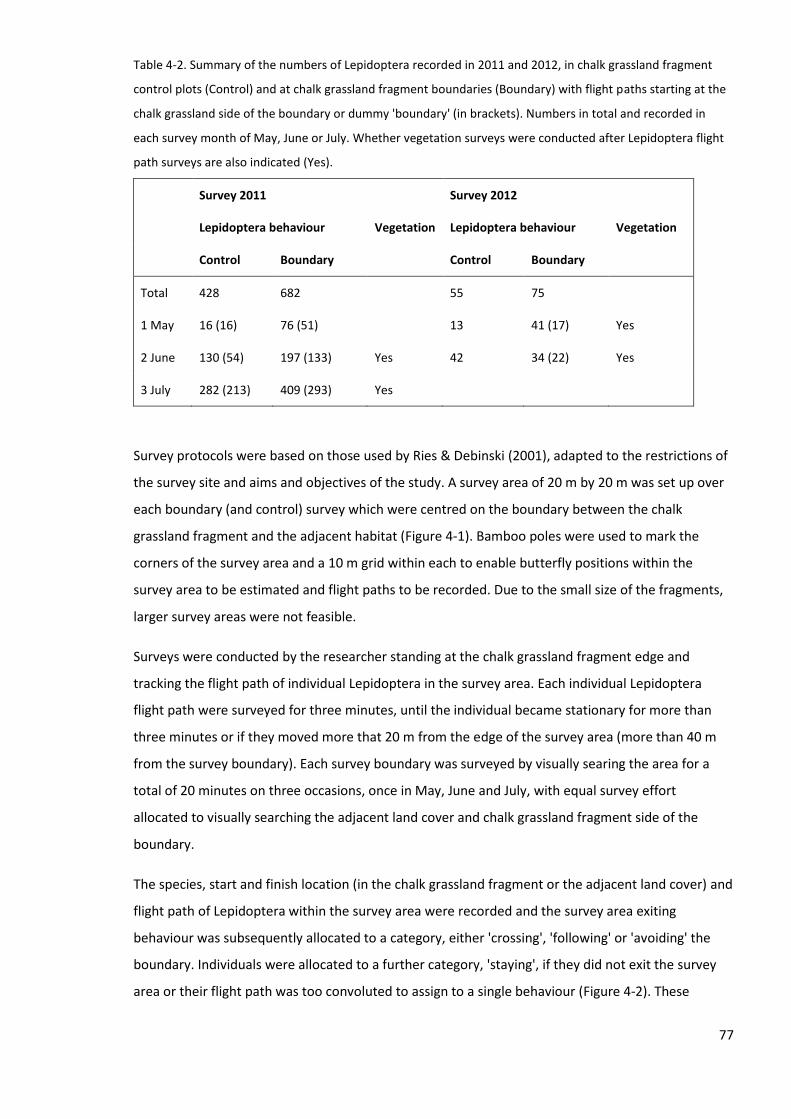
77
Table 4-2. Summary of the numbers of Lepidoptera recorded in 2011 and 2012, in chalk grassland fragment
control plots (Control) and at chalk grassland fragment boundaries (Boundary) with flight paths starting at the
chalk grassland side of the boundary or dummy 'boundary' (in brackets). Numbers in total and recorded in
each survey month of May, June or July. Whether vegetation surveys were conducted after Lepidoptera flight
path surveys are also indicated (Yes).
Survey 2011 Survey 2012
Lepidoptera behaviour Vegetation Lepidoptera behaviour Vegetation
Control Boundary Control Boundary
Total 428 682 55 75
1 May 16 (16) 76 (51) 13 41 (17) Yes
2 June 130 (54) 197 (133) Yes 42 34 (22) Yes
3 July 282 (213) 409 (293) Yes
Survey protocols were based on those used by Ries & Debinski (2001), adapted to the restrictions of
the survey site and aims and objectives of the study. A survey area of 20 m by 20 m was set up over
each boundary (and control) survey which were centred on the boundary between the chalk
grassland fragment and the adjacent habitat (Figure 4-1). Bamboo poles were used to mark the
corners of the survey area and a 10 m grid within each to enable butterfly positions within the
survey area to be estimated and flight paths to be recorded. Due to the small size of the fragments,
larger survey areas were not feasible.
Surveys were conducted by the researcher standing at the chalk grassland fragment edge and
tracking the flight path of individual Lepidoptera in the survey area. Each individual Lepidoptera
flight path were surveyed for three minutes, until the individual became stationary for more than
three minutes or if they moved more that 20 m from the edge of the survey area (more than 40 m
from the survey boundary). Each survey boundary was surveyed by visually searing the area for a
total of 20 minutes on three occasions, once in May, June and July, with equal survey effort
allocated to visually searching the adjacent land cover and chalk grassland fragment side of the
boundary.
The species, start and finish location (in the chalk grassland fragment or the adjacent land cover) and
flight path of Lepidoptera within the survey area were recorded and the survey area exiting
behaviour was subsequently allocated to a category, either 'crossing', 'following' or 'avoiding' the
boundary. Individuals were allocated to a further category, 'staying', if they did not exit the survey
area or their flight path was too convoluted to assign to a single behaviour (Figure 4-2). These
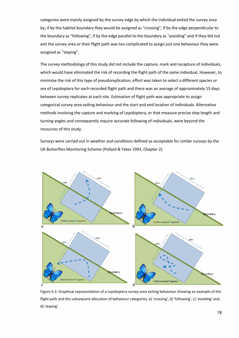
78
categories were mainly assigned by the survey edge by which the individual exited the survey area
by; if by the habitat boundary they would be assigned as "crossing", if by the edge perpendicular to
the boundary as "following", if by the edge parallel to the boundary as "avoiding" and if they did not
exit the survey area or their flight path was too complicated to assign just one behaviour they were
assigned as "staying".
The survey methodology of this study did not include the capture, mark and recapture of individuals,
which would have eliminated the risk of recording the flight path of the same individual. However, to
minimise the risk of this type of pseudoreplication, effort was taken to select a different species or
sex of Lepidoptera for each recorded flight path and there was an average of approximately 15 days
between survey replicates at each site. Estimation of flight path was appropriate to assign
categorical survey area exiting behaviour and the start and end location of individuals. Alternative
methods involving the capture and marking of Lepidoptera, or that measure precise step length and
turning angles and consequently require accurate following of individuals, were beyond the
resources of this study.
Surveys were carried out in weather and conditions defined as acceptable for similar surveys by the
UK Butterflies Monitoring Scheme (Pollard & Yates 1993, Chapter 2).
Figure 4-2. Graphical representation of a Lepidoptera survey area exiting behaviour showing an example of the
flight path and the subsequent allocation of behaviour categories, a) 'crossing', b) 'following', c) 'avoiding' and,
d) 'staying'.
a b
c d

79
Measures of vegetation characteristics and nectar flower availability were recorded for each plot
using eight, 0.5 m by 0.5 m quadrats (four on the adjacent land cover side and four on the chalk side
of the boundary chosen ad hoc). Recorded vegetation characteristics included the mean and
variation (coefficient of variation) in vegetation height and density (using the drop disc method
described by Stewart et al. 2001, henceforth referred to as vegetation density), at a rate of one drop
per quadrat) and percentage cover of bare ground. Nectar flower availability was measured as the
number of flowering units of nectar flowers, species richness and numbers of those in the
Asteraceae, Fabaceae and Dipsacaceae families. Nectar flowers were selected based on the nectar
plant database (Hardy et al. 2007). Botanical characteristics were surveyed on two occasions
between May and August.
The average wind speed and wind direction (see Chapter 4, section 5.3.3 for categorisation of wind
direction) were recorded using measurements from the nearest meteorological station at Boscombe
Down, Wiltshire, UK, which was located 6.5 km SW of the site to the nearest hour.
4.3.3 Statistical analysis
Data were analysed for all Lepidoptera regardless of species, and after categorisation into ecological
associations and mobility categories. The butterflies surveyed were grouped using ecological
classifications of species associated with: a) ruderal vegetation, b) short-grass herb-rich vegetation,
c) open grassland with medium to tall sward or warm open grassland with short-sward and, c)
woodland (Shreeve et al. 2001). The difference between the two grassland ecological groups was
that those associated with short-grass herb-rich vegetation were not dependant on grasses for any
part of their life-cycle, whereas, those associated with short, medium or tall warm open grassland
were (Shreeve et al. 2001). The larval host plants of the herb-rich grasslands associated group were
Legumes and they were likely to have a symbiotic relationship with ants. The ruderal-vegetation
group is not associated with a particular family of larval host plants, but is likely to be associated
with tall and/or mature herbs and to overwinter as pupae and the woodland group utilised trees
and/or shrubs for larval host-plants and adult feeding.
Day flying moths were categorised based on their association with different habitat types: the Six-
spot Burnet (Zygaena filipendulae) was more associated with herb-rich grassland as its larval host
plant is legume species Lotus corniculatus, (although this species will use tall grass stems and
pupation sites), the Forester moth (Adscita statices) as it is associated with herb-rich chalk grassland
where its larval host plant Common Rock-rose (Helianthemum nummularium) is abundant (Heath &
Emmet 1985). Both of these moth species were also categorised as sedentary in mobility (Naumann
et al. 1999). The Hummingbird Hawk moth (Macroglossum stellatarum) was categorised as
associated with ruderal vegetation as it is a widespread immigrant species associated with a variety
of habitat types (Heath & Emmet 1985; Langmaid et al. 1989).

80
Categories of Lepidoptera mobility used were sedentary, intermediate and widespread (Pollard &
Yates 1993). Species categorised as sedentary are unlikely to move outside the habitat patch and are
considered to have a closed population structure, whereas, species categorised as widespread are
wide-ranging and frequently move between habitat patches and have an open population structure.
species categorised as intermediate are somewhere in-between sedentary and widespread. The 6-
spot Burnet Moth (Zygaena filipendulae) was categorised as being in the sedentary mobility groups
(Naumann et al. 1999).
Wind speed was categorised by speed (Low: < 10 mph High: > 10 mph, wind direction, and
relationship to the Lepidoptera flight path direction. For example, if the Lepidoptera crossed an edge
and the wind was in the same direction it would be classed as ‘with’ the flight path (See Chapter 5,
for examples). Mean values per survey boundary (and control boundary) were calculated for
response and environmental variables. Response variables were Lepidoptera densities in total and
the different boundary behaviours. Explanatory variables were the different ecological and mobility
groups, vegetation characteristics, nectar flower availability and weather conditions.
Pearson's Chi-squared test with Yates' continuity correction and Fisher's Exact test in R (version 3.0,
R Core Team 2013) were used to compare the differences between observed and values expected
for total Lepidoptera and for each of the different ecological and mobility groups separately. The
three comparisons were;
a) between the control and boundary surveys,
b) between Lepidoptera flight paths that started in the adjacent land cover side and the chalk
grassland fragment side of the boundary.
c) between adjacent land cover types of arable land or new grassland re-creation when
Lepidoptera flight paths started in the chalk grassland fragment side of the boundary.
4.3.3.1 Comparisons between different boundary surveys and side of edge and matrix type
Differences in the observed and expected behaviours of Lepidoptera in the three comparisons were
based on; (i) the proportion that crossed the fragment boundary (or control dummy 'boundary')
compared to the proportion exhibiting other behaviours, and (ii) the proportion that followed the
boundary compared to those exhibiting other behaviours.
For comparisons between observed and expected behaviours in the survey boundaries at chalk
grassland fragments and the control boundaries in continuous land cover (comparison a) , a total of
1110 individual behaviour recordings were used. For comparisons between observed and expected
behaviours according to whether the Lepidoptera flight path observation started in the chalk
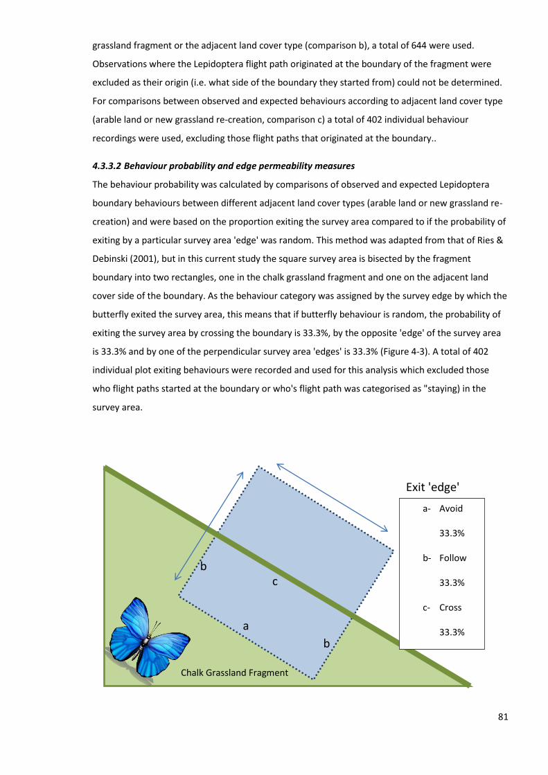
81
grassland fragment or the adjacent land cover type (comparison b), a total of 644 were used.
Observations where the Lepidoptera flight path originated at the boundary of the fragment were
excluded as their origin (i.e. what side of the boundary they started from) could not be determined.
For comparisons between observed and expected behaviours according to adjacent land cover type
(arable land or new grassland re-creation, comparison c) a total of 402 individual behaviour
recordings were used, excluding those flight paths that originated at the boundary..
4.3.3.2 Behaviour probability and edge permeability measures
The behaviour probability was calculated by comparisons of observed and expected Lepidoptera
boundary behaviours between different adjacent land cover types (arable land or new grassland re-
creation) and were based on the proportion exiting the survey area compared to if the probability of
exiting by a particular survey area 'edge' was random. This method was adapted from that of Ries &
Debinski (2001), but in this current study the square survey area is bisected by the fragment
boundary into two rectangles, one in the chalk grassland fragment and one on the adjacent land
cover side of the boundary. As the behaviour category was assigned by the survey edge by which the
butterfly exited the survey area, this means that if butterfly behaviour is random, the probability of
exiting the survey area by crossing the boundary is 33.3%, by the opposite 'edge' of the survey area
is 33.3% and by one of the perpendicular survey area 'edges' is 33.3% (Figure 4-3). A total of 402
individual plot exiting behaviours were recorded and used for this analysis which excluded those
who flight paths started at the boundary or who's flight path was categorised as "staying) in the
survey area.
Chalk Grassland Fragment
Exit 'edge'
'probability
b c
b
a
a- Avoid
33.3%
b- Follow
33.3%
c- Cross
33.3%

82
Figure 4-3. Probability of exiting the survey area for Lepidoptera on the chalk grassland fragment side of the
boundary is 33.3% for exiting the survey area by avoiding (exit at a), following (exit at b) and crossing (exit at c)
the boundary.
Edge permeability was defined as the proportion that approach the boundary and then cross it
(Stamps et al. 1987) and was calculated using the estimated flight path data recorded during the
survey. Comparisons between adjacent land cover type behaviour probabilities and edge
permeability were done for Lepidoptera flight paths that originated in the adjacent land cover side
and the chalk grassland fragment side of the boundary separately .
4.3.3.3 Logistic models
To model the effect of environmental variables on the behaviour of Lepidoptera in chalk grassland
fragments at survey boundaries for Lepidoptera in total and for the different ecological and mobility
groups, logistic stepwise regression models were conducted in R (version 3.0, R Core Team 2013)
using Generalized Linear Models (GLM) and Generalized Linear Mixed Models (GLMM) with binomial
errors. These included only Lepidoptera flight paths that originated in the chalk grassland fragment
side of the boundary and excluded Lepidoptera that did not exit the survey area and whose flight
path started at the chalk grassland fragment boundary.
GLMM used the proportion of Lepidoptera exiting the survey area as the response variable and
boundary behaviour category (cross, follow or avoid), survey month, unique survey boundary
identifier (related to position in the chalk grassland fragment and given a number 1-4), Lepidoptera
density (including those that stayed in the survey area), adjacent land cover type, wind speed and
wind direction (with or against the flight path of the individual) as explanatory variables. The
interaction of Lepidoptera density with adjacent land cover type, month with boundary behaviour
and wind speed with wind direction were also explanatory variables. These interactions are
important as behaviour can be effected by an interaction of species density, month and the strength
and direction of the wind (Ries & Debinski 2001). The unique survey boundary identifier was nested
within the location (chalk grassland fragment) as a random effect. These used fixed and random
effect; a fixed effect influences only the mean of the response variable and a random effect
influences only the variance of the response variable (Crawley 2007).
GLM used the proportion of Lepidoptera exiting the survey area and the boundary behaviour of
crossing and following were analysed separately as response variables. These included Lepidoptera
data from June and July where vegetation characteristics and nectar resources were surveyed and
therefore variables relating to vegetation density and nectar flower richness could be included in the
models. Lepidoptera behaviour results from May were excluded as they did not have corresponding
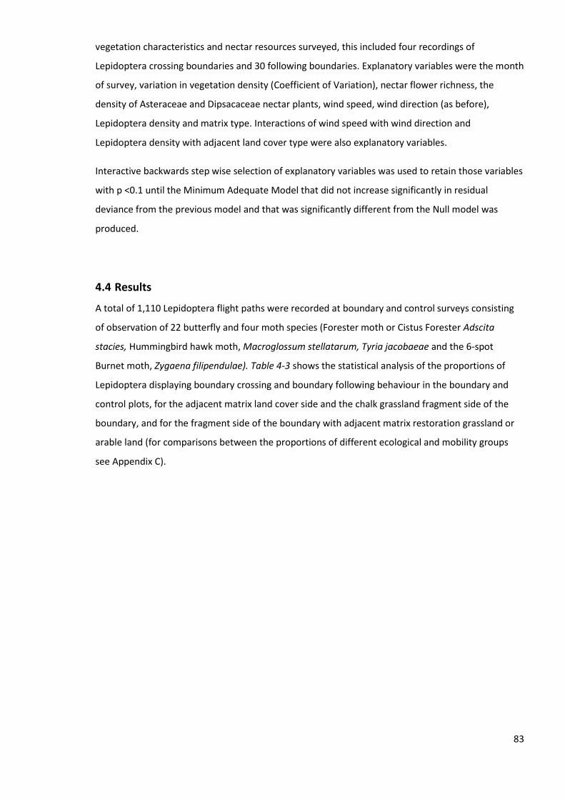
83
vegetation characteristics and nectar resources surveyed, this included four recordings of
Lepidoptera crossing boundaries and 30 following boundaries. Explanatory variables were the month
of survey, variation in vegetation density (Coefficient of Variation), nectar flower richness, the
density of Asteraceae and Dipsacaceae nectar plants, wind speed, wind direction (as before),
Lepidoptera density and matrix type. Interactions of wind speed with wind direction and
Lepidoptera density with adjacent land cover type were also explanatory variables.
Interactive backwards step wise selection of explanatory variables was used to retain those variables
with p <0.1 until the Minimum Adequate Model that did not increase significantly in residual
deviance from the previous model and that was significantly different from the Null model was
produced.
4.4 Results
A total of 1,110 Lepidoptera flight paths were recorded at boundary and control surveys consisting
of observation of 22 butterfly and four moth species (Forester moth or Cistus Forester Adscita
stacies, Hummingbird hawk moth, Macroglossum stellatarum, Tyria jacobaeae and the 6-spot
Burnet moth, Zygaena filipendulae). Table 4-3 shows the statistical analysis of the proportions of
Lepidoptera displaying boundary crossing and boundary following behaviour in the boundary and
control plots, for the adjacent matrix land cover side and the chalk grassland fragment side of the
boundary, and for the fragment side of the boundary with adjacent matrix restoration grassland or
arable land (for comparisons between the proportions of different ecological and mobility groups
see Appendix C).

84
Table 4-3. Results of comparison between observed and expected proportions of Lepidoptera displaying
boundary crossing and boundary following behaviour in total and for different ecological groups and mobility
groups of control and boundary survey areas, the chalk grassland fragment and adjacent matrix land cover side
of the boundary and at edges with adjacent matrix of restoration or arable. What plots were compared
(Compare between), behaviour tested (Behaviour), Test used (Test) Chi-Squared value (X2), significance (p=)
those p<0.05 are in bold and whether the observed proportion was higher or lower than the expected
(Comments).
Behaviour Test Test X2 p Comments
Comparison a- Edge and Control plots n=1110
Cross n=389 Cross/not Cross Chi-squared 40.94 <0.0001 Cross lower at boundaries
Follow n=434 Follow/not Follow Chi-squared 27.96 <0.0001 Follow higher at boundaries
NA Ecological group Fisher's Exact <0.0001 Open-grass proportion higher at
boundaries
NA Mobility group Fisher's Exact <0.0001 Sedentary proportion higher at
boundaries
Comparison b- Chalk and Matrix side of the edge n=644
Cross n=154 Cross/not Cross Chi-squared 75.53 <0.0001 Cross lower for those in chalk
grassland side of boundary
Ecological group Fisher's Exact 0.2159 No difference
Mobility group Fisher's Exact 0.2974 No difference
Follow n=309 Follow/not Follow Chi-squared 18.73 <0.0001 Follow higher for those in chalk
grassland side of boundary
Ecological group Fisher's Exact <0.0001 Herb-rich follow higher for those
in chalk grassland side of
boundary
Mobility group Fisher's Exact <0.0001 Sedentary follow higher for those
in chalk grassland side of
boundary
Comparison c- Restoration and Arable matrix n=402
Cross n=63 Cross/not Cross Chi-squared 8.09 0.0442 Cross higher for boundaries with
adjacent grassland re-creation
Ecological group Fisher's Exact 0.0219 Herb-rich cross higher at
boundaries with adjacent

85
grassland re-creation
Mobility group 0.0219 Sedentary cross higher at
boundaries with adjacent
grassland re-creation
Follow n=229 Follow/not Follow Chi-squared 0.52 0.4698 Follow lower for boundaries with
adjacent grassland re-creation
Ecological group Fisher's Exact 0.6229 No difference
Mobility group Fisher's Exact 0.1501 No difference
4.4.1 Comparison, a) Lepidoptera density and behaviour between boundaries and controls
Results indicate that there are differences in the proportions, behaviour and ecological or mobility
groups of Lepidoptera at survey boundaries compared to the expected values. Comparison between
observed and expected proportions of the different boundary behaviours shown by Lepidoptera and
of different ecological and mobility groups using Fisher's exact and Chi-Squared test (Table 4-3,
Figure 4-4. ) showed that there were lower Lepidoptera crossing and higher following at boundaries
than expected (X2= 40.94 and 27.96 respectively, p<0.0001). There were higher numbers of
individuals in the open-grass ecological group and in the sedentary mobility group at survey
boundaries than expected (Fisher's exact p<0.0001, Figure 4-5, Appendix C for all results).
Figure 4-4. Comparison of behaviours observed between boundary and controls survey areas, a) crossing and,
b) following Chi-squared and Fisher's Exact p<0.0001 comparing observed to expected for all. Significance
p<0.001 ***, p<0.01 **, p<0.05 *, 0.1<p>0.05 (*).
0.0
0.2
0.4
0.6
0.8
1.0
Control Boundary
Pro
po
rtio
n o
f b
eh
avio
urs
e
nco
un
tere
d
Other
Cross
a
***
0.0
0.2
0.4
0.6
0.8
1.0
Control Boundary
Pro
po
rtio
n o
f b
eh
avio
urs
e
nco
un
tere
d
Other
Follow
b
***
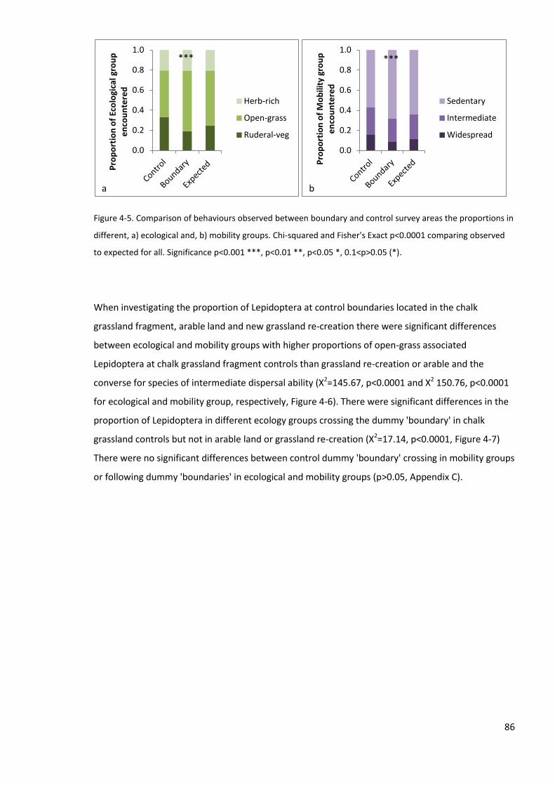
86
Figure 4-5. Comparison of behaviours observed between boundary and control survey areas the proportions in
different, a) ecological and, b) mobility groups. Chi-squared and Fisher's Exact p<0.0001 comparing observed
to expected for all. Significance p<0.001 ***, p<0.01 **, p<0.05 *, 0.1<p>0.05 (*).
When investigating the proportion of Lepidoptera at control boundaries located in the chalk
grassland fragment, arable land and new grassland re-creation there were significant differences
between ecological and mobility groups with higher proportions of open-grass associated
Lepidoptera at chalk grassland fragment controls than grassland re-creation or arable and the
converse for species of intermediate dispersal ability (X2=145.67, p<0.0001 and X2 150.76, p<0.0001
for ecological and mobility group, respectively, Figure 4-6). There were significant differences in the
proportion of Lepidoptera in different ecology groups crossing the dummy 'boundary' in chalk
grassland controls but not in arable land or grassland re-creation (X2=17.14, p<0.0001, Figure 4-7)
There were no significant differences between control dummy 'boundary' crossing in mobility groups
or following dummy 'boundaries' in ecological and mobility groups (p>0.05, Appendix C).
0.0
0.2
0.4
0.6
0.8
1.0
Pro
po
rtio
n o
f Ec
olo
gica
l gro
up
e
nco
un
tere
d
Herb-rich
Open-grass
Ruderal-veg
a
***
0.0
0.2
0.4
0.6
0.8
1.0
Pro
po
rtio
n o
f M
ob
ility
gro
up
e
nco
un
tere
d
Sedentary
Intermediate
Widespread
b
***

87
Figure 4-6. Proportions of Lepidoptera flight paths recorded of different, a) ecological and, b) mobility groups
in control survey areas in the centre of arable land (Arable) , chalk grassland fragment (Chalk) and grassland re-
creation (Grassland). Significance p<0.001 ***, p<0.01 **, p<0.05 *, 0.1<p>0.05 (*).
Figure 4-7. Proportions of Lepidoptera in different ecological groups recorded crossing the dummy 'boundary'
in control survey areas in, a) arable land for, b) in chalk grassland fragments for (c) new grassland re-creation.
Significance p<0.001 ***, p<0.01 **, p<0.05 *, 0.1<p>0.05 (*).
0.0
0.2
0.4
0.6
0.8
1.0
Pro
po
rtio
n o
f Ec
olo
gica
l gro
up
e
nco
un
tere
d
Herb-rich
Open-grass
Ruderal-veg
a
0.0
0.2
0.4
0.6
0.8
1.0
Pro
po
rtio
n o
f M
ob
ility
gro
up
e
nco
un
tere
d
Sedentarty
Intermediate
Widespread
b
***
0.0
0.2
0.4
0.6
0.8
1.0
Pro
po
rtio
n o
f b
eh
avio
urs
e
nco
un
tere
d in
Ara
ble
Other
Cross
a
0.0
0.2
0.4
0.6
0.8
1.0
Pro
po
rtio
n o
f b
eh
avio
urs
e
nco
un
tere
d in
Ch
alk
Other
Cross
b
***
0.0
0.2
0.4
0.6
0.8
1.0
Pro
po
rtio
n o
f b
eh
avio
urs
e
nco
un
tere
d in
Gra
ssla
nd
Other
Cross
c
***

88
4.4.2 Comparison, b) Lepidoptera behaviour on either side of the boundary
Results indicate that there are overall differences between the proportions of different boundary
behaviours exhibited and between different ecological and mobility groups despite the small scale of
the 20 m by 20 m survey area. For flight paths that originated in the chalk fragment side of the
boundary there were higher proportions of Lepidoptera following and lower crossing boundaries
than expected (Table 4-3, Figure 4-8, X2= 18.73 and 75.53 respectively, p<0.0001). In the chalk
grassland fragment side of the boundary there were higher proportions of open-grass and sedentary
species than expected (Fisher's Exact test, p<0.0001). Of those that crossed the boundary from the
chalk grassland fragment, there were no significant differences according to ecological or mobility
group (Fisher's Exact test, p=0.2159, p=2974, respectively). However, for those that followed the
boundary there were higher representation of herb-rich, open-grass and Sedentary species than
expected when flight paths originated in chalk fragment side of the boundary (Figure 4-9, Fisher's
Exact test, p<0.0001, Appendix C).
Figure 4-8. comparisons of behaviours according to whether the observation started in the adjacent matrix
land cover and the chalk fragment side of the boundary for, a) crossing and, b) following. Chi-squared and
Fisher's Exact p<0.0001 comparing observed to expected for all. Significance p<0.001 ***, p<0.01 **, p<0.05 *,
0.1<p>0.05 (*).
0.0
0.2
0.4
0.6
0.8
1.0
Chalk Adjacent
Pro
po
rtio
n o
f b
eh
avio
urs
e
nco
un
tere
d
Other
Cross
a
***
0.0
0.2
0.4
0.6
0.8
1.0
Chalk Adjacent
Pro
po
rtio
n o
f b
eh
avio
urs
e
nco
un
tere
d
Other
Follow
b
***

89
Figure 4-9. Comparisons of behaviours according to whether the observation started in the matrix and the
chalk fragment side of the edge for proportions in different, a) ecological and, b) mobility groups for those
individuals following edges. Chi-squared and Fisher's Exact p<0.0001 comparing observed to expected for all.
Significance p<0.001 ***, p<0.01 **, p<0.05 *, 0.1<p>0.05 (*).
4.4.3 Comparison, c) Lepidoptera behaviour to adjacent land cover of arable land or new grassland
re-creation
Results showed that an adjacent land cover of new grassland re-creation significantly increased
boundary-crossing behaviour (Table 4-3, Figure 4-10). At boundaries with grassland re-creation there
were higher proportions of Lepidoptera crossing than expected (Chi-squared, X2=8.09, p=0.0440)
and no difference between matrix types for edge following behaviour. At boundaries with grassland
re-creation there were higher proportions of Intermediate and lower of sedentary mobility groups
than expected but no difference for ecological groups (Fisher's Exact, p=0.1718). At boundaries with
grassland re-creation, there were higher open-grass ecological group and sedentary mobility group
crossing (X2= 6.17, p=0.01, and X2= 7.79, p=0.0053 respectively) and lower herb-rich associated
group crossing than expected (X2= 3.3747, p=0.0662, Figure 4-11). At boundaries with arable land
there were higher herb-rich ecological group following edges (X2= 3.23, p=0.07) than expected and
no difference for open-grass, sedentary and intermediate groups (Chi-squared, p>0.05, Table 4-3,
Appendix C).
0.0
0.2
0.4
0.6
0.8
1.0
Pro
po
rtio
n o
f Ec
olo
gica
l gro
up
fo
llow
ing
bo
un
dar
ies
Herb-rich
Open-grass
Ruderal-veg
a
***
0.0
0.2
0.4
0.6
0.8
1.0
Pro
po
rtio
n o
f M
ob
ility
gro
up
fo
llow
ing
bo
un
dar
ies
Sedentary
Intermediate
Widespread
b
***

90
Figure 4-10. Comparisons of proportions between behaviours of individuals originating in chalk grassland
fragments with adjacent land cover matrix of grassland re-creation and semi improved pasture (Grassland) or
arable land (Arable) matrix of behaviours, a) crossing and, b) following. Chi-squared and Fisher's Exact p<0.05
comparing observed to expected for all. Significance p<0.001 ***, p<0.01 **, p<0.05 *, 0.1<p>0.05 (*).
Figure 4-11. Comparisons of proportions between behaviours of individuals originating in chalk grassland
fragments with adjacent matrix of grassland re-creation and semi improved pasture (Grassland) or arable land
(Arable) matrix between, a) ecological and, b) mobility groups crossing edges. Chi-squared and Fisher's Exact
p<0.05 comparing observed to expected for all. Significance p<0.001 ***, p<0.01 **, p<0.05 *, 0.1<p>0.05 (*).
4.4.4 Behaviour probability and edge permeability measures
4.4.4.1 Behaviour probabilities
The proportion of Lepidoptera exiting the chalk grassland fragment by crossing the boundary was
lower than expected when the adjacent land cover was arable land for all Lepidoptera, herb-rich,
open-grass, and sedentary groups (Figure 4-12, p<0.05), but was not different from random when
the adjacent land was grassland re-creation. The proportion of Lepidoptera exiting the survey area
0.0
0.2
0.4
0.6
0.8
1.0
Grassland Arable
Pro
po
rtio
n o
f b
eh
avio
urs
e
nco
un
tere
d
Other
Cross
a
*
0.0
0.2
0.4
0.6
0.8
1.0
Grassland Arable
Pro
po
rtio
n o
f b
eh
avio
urs
e
nco
un
tere
d
Other
Follow
b
0%
20%
40%
60%
80%
100%
Pro
po
rtio
n o
f Ec
olo
gica
l gro
up
cr
oss
ing
bo
un
dar
ies
(%)
Short-grass
Tall-grass
Ruderal-veg
a
*
0%
20%
40%
60%
80%
100% P
rop
ort
ion
of
Mo
bili
ty g
rou
p
cro
ssin
g b
ou
nd
arie
s (%
)
Sedentary
Intermediate
Widespread
b
*

91
by following the boundary was higher than expected for both adjacent land cover types if movement
was random for all Lepidoptera and all groups except the ruderal-veg and widespread groups (Figure
4-12, p<0.05).
Figure 4-12. The proportion (%) of Lepidoptera exiting the survey area by, a) crossing the boundary and, b)
following the boundary and results of Chi-squared test to compared this proportion to the 33.33% that would
be expected if exit route was random (for example, 33% would exit the plot by crossing the edge, 33% would
exit by avoiding the edge and 33% would exit by following the edge). For Lepidoptera in total and for the
different ecological groups of ruderal-veg, herb-rich and open-grass associated species and mobility groups of
intermediate, sedentary and widespread. Significance p<0.001 ***, p<0.01 **, p<0.05 *, 0.1<p>0.05 (*).
0
10
20
30
40
50 60
70
80
90
100
Pro
po
rtio
n o
f Le
pid
op
tera
exi
tin
g p
lot
by
cro
ssin
g th
e h
abit
at b
ou
nd
ary
(%)
Lepidoptera Group
Arable
Restoration
Linear (Expected)
*** * *** ***
a
0
10
20
30
40 50
60
70
80 90
100
Pro
po
rtio
n o
f Le
pid
op
ter
exi
tin
g th
e
plo
t b
y fo
llow
ing
the
hab
itat
bo
un
dar
y (%
)
Lepidoptera Group
Arable
Restration
Linear (Expected)
*** *** *** * *** *** *** *** *** *
b

92
4.4.4.2 Edge permeability
Edge permeability values were calculated as the percentage of Lepidoptera flight paths that
approached the boundary and then crossed it. This was done for boundary crossing behaviour and
for following behaviour (approached the 'edge' of the survey area that was perpendicular to the
fragment boundary). This was calculated for flight paths originating in the chalk grassland fragment
side of the boundary (for flight paths originating in the matrix side of the chalk grassland fragment
boundary see Appendix C). Table 4-4 shows that for all ecological and mobility groups except for
ruderal-veg and widespread species, grassland re-creation had a higher permeability value which
meant that individuals were more likely to approach the boundary and then cross it. Open-grass
species had the lowest permeability to both grassland re-creation and arable edges, intermediate
species had the highest permeability to grassland re-creation edges after ruderal-veg associated
species.
Table 4-4. Mean and 1 Standard Error (SE) for boundary permeability estimates with adjacent land cover of
grassland re-creation (Grassland) and arable land (Arable) for all Lepidoptera and the different ecological and
mobility groups. Only for Lepidoptera on the chalk grassland fragment side of the boundary (see Appendix C
for the adjacent land cover side of the boundary and avoiding behaviour). This is the proportion of Lepidoptera
that approached the edge that then crossed it and compared the boundary (Crossing) to the perpendicular
edge (Following).
Response Grassland Arable Grassland Arable
Cross (%) Follow (%)
All Lepidoptera 82.46 39.01 92.78 97.75
SE 14.11 6.37 3.89 1.31
Ecological group
Ruderal-veg 66.67 83.93 100.00 88.89
SE 33.33 11.80 0.000 7.85674
Herb-rich 61.11 48.21 79.26 100.00
SE 30.93 20.49 11.57 0.00
Open-grass 51.52 22.63 65.33 98.53
SE 28.91 11.04 32.69 1.47
Mobility group
Intermediate 61.91 58.33 88.89 97.22

93
SE 31.23 22.05 5.56 2.78
Sedentary 51.52 21.67 94.00 99.29
SE 28.91 10.26 3.24 0.71
Widespread 33.33 87.50 66.67 62.50
SE 33.333 12.50 33.33 23.94
4.4.5 Modelling the behaviour of Lepidoptera
4.4.5.1 GLMM of all boundary behaviours
The Minimum Adequate Model from GLMM for all Lepidoptera in total showed that there were
higher proportions exiting the survey area by following the boundary and when there was an
interaction of month and exit behaviour with higher proportion crossing the boundary in June.
For Lepidoptera in the herb-rich ecological group there were higher proportions exiting the survey
area by following the boundary, an interaction of exit behaviour and survey month where in June
there were higher proportions crossing. For the open-grass ecological group there were higher
proportions following and lower proportions crossing boundaries.
For Lepidoptera species in the intermediate mobility group there were higher proportions crossing
and following the boundary and for the sedentary group there were lower proportions crossing and
higher proportions following. Survey month and the interaction of boundary behaviour and month
were retained in the Minimum Adequate Model but were not significant individually (Table 4-5).

94
Table 4-5. Minimum Adequate Model for GLMM for all boundary behaviours (crossing, following and
avoiding the boundary), Variable estimate, Standard error (Std.Error), z and p value. Significance
p<0.001 ***, p<0.01 **, p<0.05 *, 0.1<p>0.05 (*), See Appendix C for all model iterations.
Variables Estimate Std.Error Z p
All Lepidoptera Model iteration 8 compared to Null <0.0001 ***
(Intercept) -1.48 0.18 -8.10 <0.0001 ***
Month June -0.60 0.36 -1.69 0.0907 (*)
Month May -0.44 0.51 -0.86 0.3903
Behaviour Cross -0.14 0.26 -0.53 0.5986
Behaviour Follow 2.09 0.24 8.88 <0.0001 ***
Month June: Behaviour Cross 1.07 0.46 2.31 0.0207 *
Month May: Behaviour Cross -0.11 0.76 -0.15 0.8815
Month June: Behaviour Follow 0.60 0.44 1.38 0.1665
Month May: Behaviour Follow 1.03 0.66 1.56 0.1149
Ecological group
Ruderal-veg Null
Herb-rich Model iteration 10 compared to Null <0.0001 ***
(Intercept) -2.77 1.03 -2.69 0.0072 **
Behaviour Cross 0.76 1.28 0.59 0.5528
Behaviour Follow 4.31 1.21 3.56 0.0004 ***
Behaviour Avoid: Month June -0.78 1.45 0.541 0.5883
Behaviour Cross: Month June 1.44 0.83 1.74 0.0814 .
Behaviour Follow: Month June -1.09 0.72 -1.51 0.1318
Behaviour Avoid: Month May 1.11 1.17 0.96 0.3393
Behaviour Cross: Month May -1.16 1.27 -0.92 0.3591
Behaviour Follow: Month May -0.15 0.81 -0.19 0.8489
Open-grass Model iteration 10 compared to Null <0.0001 ***
(Intercept) -1.33 0.16 -8.12 <0.0001 ***
Behaviour Cross -0.75 0.27 -2.79 0.0053 **
Behaviour Follow 2.09 0.22 9.59 <0.0001 ***

95
Mobility group
Intermediate Model iteration 10 compared to Null <0.0001 ***
(Intercept) -3.45 0.72 -4.80 <0.0001 ***
Behaviour Cross 2.71 0.77 3.54 <0.0001 ***
Behaviour Follow 4.05 0.76 5.31 <0.0001 ***
Sedentary Model iteration 8 compared to Null <0.0001 ***
(Intercept) -1.27 0.19 -6.84 <0.0001 ***
Month June -0.52 0.39 -1.34 0.1813
Month May -0.23 0.59 -0.40 0.6905
Behaviour Cross -0.74 0.30 -2.44 0.0148 *
Behaviour Follow 1.95 0.25 7.88 <0.0001 ***
Month June: Behaviour Cross 0.85 0.56 1.51 0.1311
Month May: Behaviour Cross -16.08 2029.42 -0.01 0.9937
Month June: Behaviour Follow 0.69 0.50 1.40 0.1629
Month May: Behaviour Follow 1.06 0.82 1.29 0.1957
Widespread Null
4.4.5.2 GLM for boundary crossing
The Minimum Adequate Model from GLM for Lepidoptera crossing the chalk grassland fragment
boundary showed that there were higher proportions of all Lepidoptera crossing boundaries in May
and July, when there was a low nectar flower richness, lower variation in vegetation density, when
the wind direction was towards the chalk grassland fragment boundary, when the adjacent land
cover was new grassland re-creation and an interaction of when the wind was high and towards the
chalk fragment edge.
For Lepidoptera in the open-grass ecological group there was a higher proportion of boundary
crossing when the wind speed was low (<10 mph), when there was lower densities of other open-
grass species in the fragment but when there was an interaction of high species density at the
fragment boundary next to a grassland re-creation. For species in the sedentary mobility group there
were higher proportions crossing boundaries when species density was low or when it was high with
an interaction of adjacent grassland re-creation (Table 4-6).

96
Table 4-6. Minimum Adequate Model results from GLMs for Lepidoptera crossing the grassland fragment
boundary, Variable estimate, Standard error, z and p value. Significance p<0.001 ***, p<0.01 **, p<0.05 *,
0.1<p>0.05 (*). Appendix C for all model iterations.
Variable Estimate Std.Error Z p
All Lepidoptera Model iteration 4 compared to Null 0.0024 **
(Intercept) -0.13 1.11 -0.12 0.9037
Month July -1.31 0.50 -2.61 0.0092 **
N1 -0.38 0.18 -2.05 0.0407 *
Drop Disc CV -0.04 0.01 -2.09 0.0367 *
Wind direction towards boundary 2.43 0.88 2.77 0.0057 **
Wind speed low 1.38 0.62 2.23 0.0270 *
Adjacent grassland re-creation 1.64 0.49 3.37 0.0008 ***
Wind direction towards boundary: Wind
speed low
-2.67 1.05 -2.54 0.0110 *
Ecological group
Ruderal-veg Null
Herb-rich Null
Open-grass Model iteration 8 compared to Null 0.0018 **
(Intercept) -1.80 0.71 -2.56 0.0116 *
Wind speed low 1.28 0.66 1.95 0.0518 (*)
Open-grass Sp density -0.18 0.06 -2.92 0.0035 **
Open-grass Sp density: Adjacent
grassland re-creation
0.12 0.04 2.69 0.0072 **
Mobility Group
Widespread Null
Intermediate Null
Sedentary Model iteration 9 compared to Null 0.0115 *
(Intercept) -1.10 0.44 -2.50 0.0123 *
Sedentary Sp density -0.12 0.05 -2.39 0.0167 *
Sed Sp density: Adjacent re-creation 0.10 0.04 2.52 0.0117 *

97
4.4.5.3 GLM for boundary following
The Minimum Adequate Model of GLM for Lepidoptera following the boundary of the chalk
grassland fragment showed that there were higher proportions when nectar flower richness was
higher and lower proportions when the wind direction was towards the boundary. For species in the
herb-rich ecological group, lower proportions followed boundaries in June and when the density of
other herb-rich species was higher. For the open-grass ecological group, there was borderline
significance for higher proportions following when nectar flower richness was higher. For species in
the sedentary mobility group there was borderline significance for high proportions followed the
boundary when nectar flower richness was higher and for intermediate mobility group there was
borderline significance for lower proportions following when the wind direction was towards the
boundary (Table 4-7).

98
Table 4-7. Minimum Adequate Model results from GLMs for Lepidoptera following the grassland fragment
boundary, Variable estimate, Standard error, z and p value. Significance p<0.001 ***, p<0.01 **, p<0.05 *,
0.1<p>0.05 (*). Appendix C for model iterations.
Variables Estimate Std.Error Z p
All Lepidoptera Model iteration 9 compared to Null 0.0377 *
(Intercept) 0.02 0.32 0.05 0.9626
N1 0.28 0.12 2.30 0.0212 *
Wind direction towards boundary -0.47 0.28 -1.67 0.0953 (*)
Ecological group
Ruderal- veg Null
Herb-rich Model iteration 10 compared to Null 0.0012 **
(Intercept) 4.98 1.55 3.21 0.0013 **
Month June -2.67 1.07 -2.51 0.0121 *
Herb-rich Sp density -0.31 0.11 -2.82 0.0048 **
Open-grass Model iteration10 compared to Null 0.0692 (*)
(Intercept) -0.09 0.45 -0.20 0.8387
N1 0.28 0.16 1.78 0.0753 (*)
Mobility group
Intermediate Model iteration 10 compared to Null 0.0851 (*)
(Intercept) 0.92 0.42 2.19 0.0285 *
Wind direction towards boundary -1.00 0.59 -1.70 0.0896 (*)
Sedentary Model iteration 10 compared to Null 0.0638 (*)
(Intercept) 0.04 0.39 0.12 0.9185
N1 0.25 0.14 1.81 0.0703 (*)
Widespread Null

99
4.5 Discussion
4.5.1 Comparison of the proportions of Lepidoptera in total and of ecological and mobility groups
in different survey areas and edge permeability
Overall there were lower proportions of Lepidoptera in total crossing boundaries, and higher
proportions following boundaries than expected at chalk grassland fragment boundaries, when flight
paths originated in the chalk grassland fragment and when the adjacent land cover was arable land
(Table 4-3). This indicated that in this landscape, Lepidoptera were affected by, and responding to,
the chalk grassland fragment boundary, an effect supported by many other studies (Ries & Debinski
2001; Schtickzelle & Baguette 2003; Schultz et al. 2012).
There were significantly higher proportions of Lepidoptera crossing chalk grassland fragment
boundaries when the adjacent land cover was new grassland re-creation, when flight paths
originated in both the fragment and in the adjacent land cover side of the boundary for all
Lepidoptera (Table 4-3). A matrix that is similar in structure to the habitat patch has been shown to
have higher permeability values which increases functional connectivity. A review by (Prevedello &
Vieira 2010) summarised this affect, concluding that in 88% of studies, functional connectivity was
increased when the matrix was more similar in structure to the habitat patch. Reeve et al. (2008)
and Haynes & Cronin (2006) used experiments, observations and models of plant hoppers in habitat
patches and a matrix of different grass species and mudflat to illustrate that when the adjacent
matrix was similar in structure to the habitat edge, crossing behaviour occurred from both sides of
the edge and that the grass matrix was three times more permeable than mudflat.
Overall, grassland associated butterflies and those with sedentary and intermediate mobility groups
responded similarly to chalk grassland fragment boundaries with lower proportions crossing and
higher proportions following than expected if movement was random. This was supported by the
behaviour probabilities results whereby, these groups crossed significantly less at boundaries with
adjacent arable land but was no different from random when there was adjacent new grassland re-
creation. This is likely to be because they are associated with grasslands for larval hot plants and
nectar sources they are more reluctant to leave an area which contains the resources they require.
Those in the ruderal-veg ecological and widespread mobility groups did not show a similar significant
trend to the other groups as these species are less specialist in their habitat requirement and not
ecologically restricted to grassland habitats (Langmaid et al. 1989), therefore these groups will not
be discussed further.
There were some differences between these groups, indicating that new grassland re-creation may
be more effective for some groups. An adjacent matrix type of new grassland re-creation affected
the herb-rich ecological and the sedentary groups with significantly higher proportions crossing

100
when boundaries were adjacent to this matrix type, indicating the importance of even this new
habitat on the behaviour of these group. Although, herb-rich associated Lepidoptera species had
higher overall permeability values at boundaries, there were lower proportions crossing and more
following boundaries than expected and this may have been a result of those individuals in the
survey areas were more likely to cross whereas others may have already avoided the boundary
before they entered the survey area and this is supported by the fact that there were significantly
higher proportions of open-grass group and lower proportions of herb-rich at boundaries.
A chalk grassland fragment boundary with an adjacent land cover of grassland re-creation was more
permeable than one adjacent to arable land for all grassland ecological and intermediate to low
mobility groups (Table 4-4). Chalk grassland fragment boundaries adjacent to grassland re-creation
had the highest permeability value for the herb-rich ecological group and sedentary mobility group.
These results support similar results reported for the Mountain Parnassian butterfly (Parnassius
smintheus) where the forest matrix was twice as resistant to movement as meadows (Matter &
Roland 2002). Also for the specialist prairie Lepidoptera species the Regal Fritillary (Speyeria idalia)
where significantly different crossing than expected was reported when the matrix land cover was
crop and/or field (Ries & Debinski 2001).
Results considering the permeability of the chalk grassland fragment boundary to Lepidoptera
located in the adjacent land cover showed higher permeability values compared to those in the chalk
grassland fragment especially for open-grass ecological and Sedentary mobility groups (Appendix C).
This is unlikely to represent species immigration into the chalk grassland fragment and more likely
due to foray loop behaviour where Lepidoptera will cross the habitat boundary and fly into the
matrix for some distance before returning to the habitat. This behaviour has been studied in
Maniola jurtina and Pyronia tithonus (Meadow brown and Gatekeeper butterflies respectively,
open-grass ecological and sedentary mobility groups) where 70%-80% of edge crossing behaviours
were foray loops (Conradt & Roper 2006) and similarly in Delattre et al. (2010a) showed that
although 27% of Maniola Jurtina went into the arable matrix, 16% were foray loops. This means that
edge permeability can’t be used as a measure of dispersal or connectivity alone but this behaviour is
at least the first step in dispersal.
There were reasonably high permeability values for boundaries with adjacent arable land for herb-
rich associated and intermediate mobility Lepidoptera (48% and 58%, respectively, Table 4-4). There
were also high permeability values for the boundaries when Lepidoptera from these groups were
recorded in the arable land cover as a high proportion crossed back over to the chalk grassland
fragments (Appendix C). This may be attributed to the foray loop behaviour descried in Maniola
jurtina (Delattre et al. 2010a). However, due to the survey methodology, the mechanism behind this
101
result cannot be determined as butterfly flight paths were not surveyed for more than 40 m from
the habitat boundary.
There were some differences between the grassland associated mobility groups and the sedentary
and intermediate mobility groups. For flight paths that originated in either the chalk grassland
fragment or the adjacent land cover side of the boundary, there was no difference for ecological or
mobility groups that crossed boundaries. However, for those that followed boundaries, there were
higher proportions of herb-rich associated Lepidoptera and the sedentary mobility group and lower
proportions of intermediate mobility Lepidoptera (Table 4-3). Also for boundary permeability values,
there were lower permeability values for open-grass group compared to the herb-rich group and
lower permeability for sedentary compared to intermediate
Boundary response, behaviour probabilities and boundary permeability values differ between
ecological and mobility groups, these results are supported by a review by (Prevedello & Vieira 2010)
which showed that matrix land cover type effects are species specific and even closely related
species of butterfly respond to matrix differently (Ricketts 2001). For example, Ries & Debinski
(2001) showed that the more prairie specialist Lepidoptera species, Speyeria idalia had significantly
different proportions of crossing behaviour than expected when the matrix was crop and field with a
quarter of individuals crossing edges that had first approached them, however for the more
generalist species, Monarch butterfly (Danaus plexippus) edge crossing behaviour did not differ from
expected and doubled in edge permeability values.
4.5.1.1 limitations
The grouping of all species together does not allow for the species specific differences to be
identified, however grouping does allow for robust statistical analysis and grouping into ecological
associations and mobility does enable for differences between species that have similar life history
traits to be analysed and rare species to be include. For this study arable land of either oil-seed rape
or winter wheat was grouped due to low replication, however, it is likely that there would be
differences between butterfly behaviour at these two matrix types as oil-seed rape can provide early
flowering sources of nectar for many nectar feeding insects (Bartomeus et al. 2014; Riedinger et al.
2014; Woodcock et al. 2013) as well as microclimate an larval host plants for Pieris. sp. of butterfly
(Langmaid et al. 1989).
4.5.1.2 Summary
Overall, behaviour of Lepidoptera in and at boundaries of grassland re-creation which was only 1 or
2 years old was significantly different from arable for all grassland and intermediate to low mobility
groups indicating that this new habitat can encourage the dispersal of these groups.

102
Lepidoptera boundary crossing behaviour is affected by many variables and not just the type of land
cover adjacent to habitat patches, behaviour may also be affected by vegetation characteristics,
nectar and host plant resources, and the month of study, weather conditions and co-specific density
for example and these variables are discussed below.
4.5.2 Environmental variables that increased the proportion of Lepidoptera crossing edges
Models showed the importance of new grassland re-creation adjacent to chalk grassland fragments,
a low variation in vegetation structure, nectar richness, the effect of weather (wind direction) and
density dependence on Lepidoptera behaviour at chalk grassland fragment boundaries (Table 4-5,
Table 4-6, Table 4-7).
A low variation in vegetation structure as measured by vegetation density, low nectar flower species
richness across the boundary and an adjacent land cover of grassland re-creation were significant
explanatory variables (variables indicating a similar structure and nectar flower composition to the
chalk grassland fragments) for all Lepidoptera with a positive effect on the proportion crossing
boundaries (Table 4-5, Table 4-6, Table 4-7). An increase in nectar flower species richness increased
the proportion of herb-rich Lepidoptera following boundaries, this potentially indicates that there
were different nectar sources in the adjacent land cover to the chalk grassland fragment which
weren't attractive to this group. This is an interesting result, especially as the surveys in Chapter 3
have shown that these new grassland re-creation fields at the Stonehenge Landscape are providing
many nectar resources and some host plant for Lepidoptera ). Overall, butterfly species richness is
positively affected by plant species richness (Rosin et al. 2012) and variables effecting the dispersal
and as a result the abundance and richness of Lepidoptera in habitat patches in fragmented
landscapes are affected by the quality and abundance nectar flowers (Binzenhofer et al. 2005;
Clausen et al. 2001; Matter & Roland 2002) and host plant patches (Berg et al. 2011; Heer et al.
2013; Menendez et al. 2002; Schultz et al. 2012). The effect of floral resources is species-specific and
not all species will respond, (Clausen et al. 2001; Ricketts 2001). For example Clausen et al. (2001),
showed that the abundance of Skippers (Thymelicus sp.) and Ringlet (Aphantopus hyperantus) were
positively affected by the number of nectar plants but the abundance of Maniola jurtina was not,
despite these species all belonging to the same open-grass ecological and sedentary mobility group.
Model results showed no effect of the density of nectar plants in the Asteraceae and Dipsacaceae
families in contrast to previous results (Chapter 3) and other studies for example, composite nectar
flowers (Ricketts 2001) and nectar plant species of Field Scabious (Knautia arvensis), Small Scabious
(Scabiosa columbaria), Greater Knapweed (Centurea scabiosa), Thistles (Cirsium. sp) and Mouse-ear
Hawkweed (Hieracium pilosella) (Binzenhofer et al. 2005; Clausen et al. 2001). Similarly, the effect of
vegetation height on butterfly presence is dependent on species specific preferences. For example,
the abundance of Aphantopus hyperantus was positively affected by increased vegetation height

103
and species that were less mobile were more significantly affected than more mobile species
(Clausen et al. 2001).
Models showed that when the wind was with the direction of the crossing flight path, a higher
proportion crossed than expected and this is supported by results from generalist Lepidoptera
Danaus plexippus (Ries & Debinski 2001). Temperature and solar radiation are also important for
butterflies which are thermoregulating insects shown in studies where immigration can be
dependent on temperature (Ricketts 2001) and the abundance and site (habitat patch) occupancy
can be associated with rates of solar radiation at sites (Clausen et al. 2001; Heer et al. 2013). Models
also highlighted more crossing and less avoiding behaviour for herb-rich Lepidoptera in July most
likely Common Blues (Polyommatus icarus) which emerged at the end of May and then August,
perhaps low numbers of individual in July increased crossing behaviours and this is supported by the
generalist Danaus plexippus where boundary crossing was affected by survey week with more
crossing at the end of the season (Ries & Debinski 2001). Conversely, some studies have shown that
flight times can be significant in explaining differences in abundance and species richness between
habitat types for the early season (May to the middle of June) (Berg et al. 2011). More crossing
behaviour in July also coincided with lower total numbers of nectar flowers in July compared to June
across the survey area (mean 14.0 and 41.5, respectively) and lower nectar flower species richness
(mean 2.6 and 3.2, respectively, data not shown), the main contributor to this was nectar flowers in
the Fabaceae family which had higher abundance in June compared to July (9.3 and 0.4,
respectively) and potentially individuals were crossing more to find additional nectar resources.
Models showed that as the Lepidoptera ecological or mobility group density in the survey area
decreased there was an increase in the proportion of Lepidoptera crossing for open-grass and
Intermediate groups except when group density was high at boundaries with adjacent grassland re-
creation which increased the proportion crossing. Similarly, Alpine meadow species Mountain
Parnassian (Parnassius smintheus) were more likely to stay at habitat patches with high numbers of
conspecifics (members of the same species) and migrate when there were low numbers (Roland et
al. 2000) and for the prairie specialist Speyeria idalia plot exiting was affected by a species density
interaction with habitat types where crossing was less likely as co-specific density increased and
higher when the matrix was a grassy field than when it was crop or woodland (Ries & Debinski 2001).
The effect of density dependence varies between species and depends on the sex of the individual,
for example, immigration of the male alpine meadow butterfly Parnassius smintheus was positively
affected by number of females (Matter & Roland 2002).
4.5.2.1 Limitations
Models did not consider aspects of the surrounding landscape, for example measures of fragment
connectivity or the different habitat types in the landscape and studies have shown that these

104
aspects are important for example, site/patch occupancy for Iolas Blue (Iolana iolas) was dependent
on connectivity (Heer et al. 2013), Zygaena filipendulae presence was dependant on dry grassland
close by (Binzenhofer et al. 2005) and linear features in the landscape such as hedgerows, lanes and
grassy field margins are important for Lepidoptera abundance (Clausen et al. 2001; Delattre et al.
2013). Also shelter and woodland are important, for example, Lepidoptera species richness and
abundance were affected by shelter (Rosin et al. 2012) and Maniola jurtina were affected by shelter
and tree species (Clausen et al. 2001). The management of the landscape is also important such as
the type and intensity of grazing (Clausen et al. 2001). Additionally, patch size may be an important
variable as there may be more crossing in smaller patches a individuals are more likely to encounter
an edges, however studies have shown that behaviour that the probability of encountering an edge
is related to the probability of crossing it (Conradt et al. 2000; Conradt & Roper 2006).
Weather conditions can be important at effecting butterfly behaviour however, microclimate too is
very important especially considering the ground temperature for oviposition and thermoregulation
(Beyer & Schultz 2010) and this study did not sure this variable, this mean that future studies would
benefit from this additional variable .
These results show that not all groups respond similarly to chalk grassland fragments boundaries
and different environmental variables, there is also difference within species with males and females
responding differently, an aspect that was not analysed in this study as a sex could not be allocated
to all individuals in the passive observational study. Even though males and females may respond to
resources and structural similarly e.g. vegetation density, the strength of the response, movement
rates, foraging strategy and flight characteristics may differ. Studies have shown that females are
more affected by resources and males by habitat types (Schultz et al. 2012) and for Adonis Blue
(Lysandra bellargus) even though there was high selectivity in both males and females for nectar
plants but their foraging strategies were different, females utilised a higher range of nectar plants
but in a shorter distance to the habitat patch than males (Rusterholz & Erhardt 2000). For Parnassius
smintheus, 52% of males and 35% females moved between meadows (Matter & Roland 2002).
4.5.2.2 Summary
Boundary crossing and following behaviour was influenced by a mixture of vegetation characteristics
such as vegetation density and nectar plant availability, weather conditions and group density.
Results show that boundaries with similar vegetation density and nectar plant species to the habitat
fragment can encourage crossing behaviour. Some of these variables could be managed for example,
flowering plant species richness and structural similarity of restoration habitat patches to reflect that
of the target habitat and source fragments. The different responses of ecological and mobility
groups indicate that managing habitat patches and landscape for heterogeneity is also important.

105
4.6 Conclusion
The results from this study illustrate the utility of new grassland re-creation adjacent to chalk
grassland fragments. There were significantly higher proportions of Lepidoptera associated with
grasslands and low to intermediate mobility groups crossing boundaries at new grassland re-creation
compared to if movement and therefore behaviour was random. This indicates that grassland re-
creation that was only 1-2 years old was significantly different from arable land when Lepidoptera
boundary behaviour was investigated and therefore may increase the functional connectivity of
isolated habitat patches. There were higher proportions of herb-rich associated Lepidoptera crossing
at boundaries with adjacent grassland re-creation, than the open-grass associated group. However,
higher proportions of species associated with herb-rich habitats followed rather than crossed
boundaries and therefore were potentially more isolated to the chalk grassland fragments.
Results showed that variables relating to vegetation characteristics and nectar resources may
increase boundary crossing behaviour and these could be managed for. However, specialist species
would require either targeted management or more time for restoration grasslands to mature,
before functional connectivity was enhanced for this group.
106
Chapter 5 The effects of mowing on the boundary behaviour of two grassland
associated Lepidoptera species
5.1 Introduction
The behavioural response of an individual to features of a fragmented landscape is dependent on
species traits, their functional group and landscape context (Debinski & Holt 2000; Prevedello &
Vieira 2010; Ricketts 2001; Ries & Debinski 2001; Steffan-Dewenter et al. 2002). It is important to
understand how these behavioural responses change with habitat loss, fragmentation and climatic
and land use change in order to predict future behaviour and make recommendations for
conservation actions. Boundary features can also be important for habitat, resources and dispersal
for many insect species, for example, crop edges and grassy margins (Delattre et al. 2010b; Driscoll &
Weir 2005; Ouin et al. 2008).
Examining behaviour at habitat boundaries can give insights into dispersal, immigration and
emigration rates as, for an individual, crossing a habitat boundary is the first factor in dispersal
(Clobert et al. 2004). Management practices and spatial targeting of habitat restoration can be used
to encourage certain types of behaviour such as boundary crossing by increasing the permeability of
the adjacent matrix (for example, Haynes & Cronin 2003). Conservation approaches can also take
account of certain types of behaviour such as boundary following and the usage of linear features as
corridors (for example, Berggren et al. 2001; Driscoll & Weir 2005; Duelli & Obrist 2003; Ockinger &
Smith 2007b).
Behaviour at habitat boundaries has been studied in observational studies in real landscapes
(Conradt & Roper 2006; Delattre et al. 2013; Matter & Roland 2002; Pither & Taylor 1998; Ries &
Debinski 2001) and in experiment settings (Haynes & Cronin 2006; Reeve et al. 2008). In
observational studies it is difficult to control for environmental and landscape variables at different
sites and therefore experiments can be used to investigate boundary behaviour whilst controlling for
these variables. However, the transferability of results derived from experimental set ups may be
limited to the species, habitat and landscapes studied. Additionally, some behaviour can be
misleading, for example, not all crossing behaviour will result in immigration, for example, some
butterflies exhibit foray loop behaviour where they will cross a habitat boundary, fly through the
matrix for a few metres and then return to the original habitat patch (Conradt & Roper 2006;
Delattre et al. 2010a).

107
Management of grasslands influences their conservation value especially grazing and mowing
regimes which have a significant effect on plant and insect species richness, community
compositions and interactions (Buri et al. 2013; Clausen et al. 2001; Maccherini & Santi 2012). The
structural similarity of habitat and matrix land cover is a key component in increasing matrix
permeability and therefore increasing the colonisation of new habitat patches . timing and extent of
mowing and grazing should be late and varied in order to increase insect biodiversity (Berg et al.
2013; Lenoir & Lennartsson 2010), leaving uncut refuges utilised by many insect species (Berggren et
al. 2002; Buri et al. 2013; Humbert et al. 2012).
To explore boundary behaviour the Stonehenge World Heritage Site (WHS), Wiltshire, UK (see
Chapter 2) was used as the study site. Here, over 500 hectares of species-rich grassland are being re-
created and restored on former arable land. These ex-arable fields have been sown with species-rich
locally-sourced chalk grassland seed mixtures from the year 2000 to 2012, creating a
chronosequence of grassland re-creation fields across the landscape.
The Meadow Brown (Maniola jurtina) butterfly is used as an indicator and model species in
experiments (Conradt et al. 2000; Delattre et al. 2010a; Merckx et al. 2003) due to high local
abundance in fragmented agricultural landscapes, wide distribution, and reliance on grassland
habitats (Asher et al. 2001; Shreeve et al. 2001).The 6-spot Burnet moth, Zygaena filipendulae
occurs in species-rich grasslands where its larval host plant Bird's-foot Trefoil (Lotus corniculatus)
(Heath & Emmet 1985) and pupation sites (often long grass stems) are abundant, but has been less
widely used as a study organism (but see Menendez et al. 2002). These species were the most
abundant on the study site at the time of the experiment. Other species were recorded but data
were combined in an 'all Lepidoptera species' category due to low individual species abundances in
order to allow for statistical analysis.
5.2 Aims and Hypotheses
Aims;
To investigate Lepidoptera behavioural response to small scale alterations in habitat
structure at experimental boundaries.
To determine whether Lepidoptera response to the physical attributes of the mown
boundary itself or the lack of resources in the mown area.
To determine if there are differences in boundary behaviour between Lepidoptera species.
To inform the spatial targeting of grassland re-creation.

108
Hypotheses;
i. Mowing will reduce boundary crossing behaviour and increase boundary following and
avoiding behaviour.
ii. Behaviour at mown boundaries will be species specific due to differences in larval host-plant
specialism and mobility.
iii. Differences in behaviour at mown boundaries will be due to difference in structure rather
than lack of resources.
5.3 Methods and materials
5.3.1 Experimental set up
The experiment was set up in the Seven Barrows grassland re-creation field which was sown with
chalk grassland seed sourced from Salisbury Plain in 2000 (Figure 5-1, Chapter 2), this field was
species-rich and was the most similar in plant community assemblages to the chalk grassland target
habitat. Here, two large areas of grassland (40 m by 50 m) were mown and eight 20 m long survey
boundaries were set up and given a unique boundary identifier number from 1-8. Four of these were
set up on the edge of one of two mown areas (treatment boundaries) and four were set up in areas
of continuous un-mown grass which had dummy 'boundaries' parallel to the mown boundaries
(control boundaries, Figure 5-2). Two 'blocks' were set up, one next to a small fragment of woodland
with the un-mown side of the boundary to the west , and the other with the un-mown side of the
boundary to the east; these are referred to as 'sheltered' and 'exposed' block respectively (Figure
5-2). The two mown areas were 15 m from one another, treatment boundaries within the same
block were separated by 5 m, control boundaries within the same block were separated by 5 m and
treatment and control boundaries were separated by 25 m (Figure 5-2). Boundaries were surveyed
from 24th July- 23rd August 2012.
The close proximity of the survey boundaries and blocks aimed to minimise the variation in grassland
species composition, structure and climatic conditions, and was designed to fit within the area that
was allocated for the experiment by the tenant farmer. To reduce the impact of the experiment on
ongoing and subsequent sheep grazing in the field, the tenant farmer limited the area of mown grass
to no more than 400 m2 (0.04 hectares) in total and a fenced off experimental area of no more that
100 m across. The main limitations of this experimental set up were that treatment survey
boundaries were 2.5 m from the perpendicular edge of the mown area and that there was a
minimum distance of 15 m from survey boundaries and the fences in the field (Figure 5-2).This
means that Lepidoptera may have been responding to the perpendicular edge of the mown area at

109
transect boundaries and/or the fences at control boundaries. Treatment boundaries were located in
the centre of the field to minimise the possible confounding effects of the fences and woodland.
Figure 5-1. The location of the Seven Barrows grassland re-creation field (sown in the year 2000) within the
National Trust Stonehenge Landscape in 2012 and the set up of the experimental survey boundaries within the
Seven Barrows field. Treatment survey boundaries located at the edge of the mown area and control survey
dummy 'boundaries' in continuous grassland.
Survey protocols were based on those used by Ries & Debinski (2001), adapted to the survey site
and aims and objectives of the study. Treatment boundary surveys were conducted at the edge of
the mown area and control boundary surveys were conducted on the corresponding dummy
'boundary' and the area surveyed was 10 metres either side of the 20 m survey boundary (survey
area of 20 m by 20 m). Bamboo poles were used to mark the corners of the survey area and a 10 m
grid within each to enable butterfly positions within the survey area to be estimated and flight paths
to be recorded (method also described in Chapter 4). The characteristic flora of the experimental
area was associated with species-rich chalk grassland, most similar to the Upright Brome dominant
grassland community (Bromopsis erecta grassland, CG3 in Rodwell 1992) with Quaking Grass (Briza
media), Glaucous Sedge (Carex flacca), Ribwort Plantain (Plantago lanceolata) and Bird's-foot Trefoil
(Lotus corniculatus) constant throughout the sward as well as a high abundance of Sainfoin
(Onobrychis viciifolia) which is not characteristic of a chalk grassland community but successfully
established in this re-creation filed (Campbell 2009; Pemberton 2011).
Map produced by Grace Twiston-Davies
2013 © Natural England copyright (2013).
Contains Ordnance Survey data © Crown
copyright and database right 2013.
LCM2007 © and database right NERC
(CEH) 2011. All rights reserved. © third
party licensors.

110
Figure 5-2. Schematic of the experimental set up of survey boundaries (not to scale) in the , a) Sheltered Block
(un-mown side to the west) and, b) Exposed block (un-mown side to the East). Four control survey boundaries
(1-4) with dummy 'boundaries' shown for control and four treatment survey boundaries (5-8) with the mown
area adjacent. For controls the 'mown' side of the boundary was to the east in the 'sheltered' block and to the
west in the 'exposed' block. The close proximity of survey boundaries to each other and to fences aimed to
minimise within site variation and fit the experimental design within the area that was allocated for the
experiment although does require careful interpretation of results.
Mown area
'Exposed' Block
Dummy 'boundary'
20
m
40 m
50
m
5 m
25 m
2.5
m
2.5
m
Fen
ce
20 m
Un-mown area
6
5
2
1
b
Mown area
'Sheltered' Block
Dummy 'boundary'
20
m
40 m
50
m
5 m
25 m
2.5
m
2.5
m
Wo
od
lan
d
15 m
Un-mown area
4 8
3 7
Fen
ce
a

111
For survey boundaries in the 'exposed' block the un-mown side of the boundary was on the on the
east side of the boundary and therefore on the east side of control in that block. For survey
boundaries in the 'sheltered' block the un-mown side of the boundary was on the west side of the
boundary and therefore the west side for the control for that block.
5.3.2 Lepidoptera surveys
The survey was conducted by the surveyor standing at the survey boundary (or dummy 'boundary' in
controls) and tracking the flight path of individual Lepidoptera in the area 10 m either side of the
survey boundary. Each individual Lepidoptera flight path was surveyed for three minutes, until the
individual became stationary for more than three minutes, moved further than 20 m from the edge
of the survey area (Lepidoptera returning to the survey area could also be recorded). Each boundary
was surveyed for a total of 20 minutes on three occasions over the five week period (referred to as
survey period). The sequence of boundaries surveyed was chosen randomly and equal survey effort
was allocated to visually searching both sides of the boundary. The order and time of day for
surveying each survey area was random so to spread surveys throughout the survey period and
throughout the day.
The species, start and finish location (in the un-mown or mown side of the boundary or the
corresponding control 'boundary') and flight path of Lepidoptera within the 20 m by 20 m survey
area around were recorded. The behaviour by which the Lepidoptera exited the 20 m by 20 m survey
area was categorised as either 'crossing', 'following' or 'avoiding' the boundary (or dummy
'boundary'). Individuals were allocated to a further category, 'staying', if they did not exit the survey
area or their flight path was too convoluted to assign to a single behaviour.
For each survey period, each boundary survey (boundaries 1-8) were completed before the next
survey period began, the first being was between 24th July-9th August , the second between 10th-
11th August and the third between 14 -23rd August. This was a short window of the overall butterfly
flight season but coincided with the peak abundance of adult (imago) Maniola jurtina and Zygaena
filipendulae at the Stonehenge landscape which were shown in previous transect surveys from 2010-
2011 (Chapter 3, the peak occurrence for both of these species were the last week in July to the first
week in August, data not shown), although imago of both of these species may start emerging from
pupa from June. The number of days it took to complete each survey period varied as was
dependant on weather conditions. There was an average of 10 days between each survey at the
same survey transect throughout the study minimising the possibility of pseudoreplication by
recording the flight path of the same individual which may have been increased by the close
proximity of survey transects and blocks in the experiment.

112
Surveys were carried out in weather and conditions defined as acceptable for similar surveys by the
UK Butterflies Monitoring Scheme (Pollard & Yates 1993).
5.3.3 Environmental variables
Measures of vegetation characteristics and nectar flower availability were recorded for survey area
(20 m by 20 m) using eight, 0.5 m by 0.5 m quadrats placed in homogenous vegetation
representative of the survey area (four in the un-mown side of the boundary, four in the mown side
and the corresponding sides of the control dummy 'boundary'). Recorded vegetation characteristics
included the mean and variation (coefficient of variation) in vegetation height and density (using the
drop disc method described by Stewart et al.,(2001) 1 drop per quadrat, henceforth referred to as
vegetation density). Nectar flower availability was measured as the number of flowering units of
nectar flowers, species richness and numbers of those in the Asteraceae, Fabaceae and Dipsacaceae
families. Nectar flowers were selected based on the nectar plant database ((Hardy et al. 2007).
Botanical characteristics were surveyed on three occasions (19th July, 10th August and 23rd/24th
August).
Variables relating to vegetation height and density and the coverage of bare ground and leaf litter
are important for butterflies, as they effect the microclimate and can be used as a resource for
oviposition, pupation, courtship and thermoregulation (e.g. Beyer & Schultz 2010; Lawson et al.
2014; NCC 1986; Thomas et al. 2009). Different butterfly species are associated with different
vegetation heights (NCC 1986) for example, the recovery of a threatened Butterfly species, the Large
Blue (Maculinea arion) can be determined by the vegetation height as this effects the microclimate
and the subsequent establishment of a successful symbiotic relationship (Thomas et al. 2009). The
cover and height of grasses and depth of leaf litter can determine the selection of oviposition sites
for Skipper species (Pokes mardon) (Beyer & Schultz 2010) and in cooler sites, bare ground may
provide a warmer microclimate for oviposition site for Heperia comma (Lawson et al. 2014).
The average wind speed and wind direction were recorded using measurements from the nearest
meteorological station at Boscombe Down, Wiltshire, UK (Chapter 2) to the nearest hour; cloud
coverage by eye and average microclimate conditions of humidity, wind speed and air temperature
using a digital recorder held at one metre from the ground for three minutes at the start of the
survey.
Wind direction was categorised by the relationship to the boundary. For example, if the wind was in
the same direction or less than 45 it would be classed as 'with' the orientation of the boundary , if
the wind was in the opposite direction or equal to or more than 45 to the boundary it was classed
as 'against' (Figure 5-3).

113
Figure 5-3. Examples of how the relationship of wind direction and boundary edge was categorised as the wind
either with or against the orientation of the survey area boundary. If the wind direction was less than 45 to
the boundary than it was categorised as "with" the boundary orientation and if it was equal or more than 45
it was categorised as "against" the boundary orientation.
5.3.4 Statistical analysis
The mean values per survey boundary were calculated for the following response variables: total
number of Lepidoptera, Maniola jurtina and Zygaena filipendulae and different survey area exiting
behaviours. Mean values were also calculated for the explanatory variables of weather,
microclimate, nectar resource and vegetation characteristics. These were calculated for each survey
boundary overall and for each side of the survey boundary (mown and un-mown side of the
treatment boundary and the corresponding 'mown' and un-mown side of the control dummy
'boundary'). Statistical comparison was conducted using Pearson's Chi-squared test with Yates'
continuity correction and Fisher's Exact test in R (version 3.0, R Core Team 2013) and Students T-test
(Wilcoxon sum rank for non normal distribution) for Lepidoptera/environmental variables in:
a) either side of the boundary (whole survey area) between;
i. treatment boundaries and control boundaries,
ii. the 'sheltered' and the 'exposed' block,
Boundary
Wind direction in relation to boundary
With
Against

114
b) in the un-mown side of the treatment boundary or corresponding side of the dummy
'boundary' between;
i. treatment boundaries and control boundaries,
ii. the 'sheltered' and the 'exposed' block,
c) in the un-mown side of the boundary compared to the mown (or 'mown' side for control
dummy 'boundaries') side of the boundary for treatment and control boundaries separately.
5.3.5 Behaviour probability and boundary permeability measures
The probability of different behaviours and boundary permeability were measured for all
Lepidoptera and for Maniola jurtina and Zygaena filipendulae separately and used the methodology
described in Chapter 4.
Behaviour probabilities were calculated by comparing observed and expected proportions of survey
area exiting behaviours (by crossing, following or avoiding the boundary) at treatment and control
boundaries. This method was adapted from that of Ries & Debinski (2001), but in this study the
square survey area was bisected by the boundary or dummy 'boundary' into two rectangles, one in
the un-mown side of the boundary and one in the mown side (and corresponding 'mown' sides for
controls). As the behaviour category was assigned by the survey edge by which the butterfly exited
the survey area, this means that if butterfly behaviour is random, the probability of exiting the
survey area by crossing the boundary is 33.3%, by the opposite 'edge' of the survey area is 33.3%
and by one of the perpendicular survey area 'edges' is 33.3% (Figure 5-4).

115
Figure 5-4. Probability of exiting the survey area on the un-mown side of the boundary is 33.3% for exiting by,
avoiding (exit at a), following (exit at b) and crossing (exit and c) the survey boundary.
Boundary permeability was defined as the proportion that approach the boundary and then cross it
(Stamps et al. 1987) and was calculated using the estimated flight path data recorded during the
survey.
Comparisons between behaviour probabilities and boundary permeability were done for flight paths
that originated in the un-mown and mown side of the boundary separately (or corresponding
control side of the dummy 'boundary').
5.3.6 Generalised Linear Mixed Models
To investigate the differences between Lepidoptera behaviour at the mown boundaries and on
either side of the boundaries, two models were created that used all Lepidoptera responses on both
sides of the boundary and just those on the un-mown or corresponding side of the control
boundaries. This also enabled the effect of wind speed and direction to be investigated. The
proportion of all Lepidoptera, Maniola jurtina and Zygaena filipendulae crossing boundaries and
following boundaries separately were response variables in two different Generalised Linear Mixed
Models (GLMM, Table 5-1). These used fixed and random effect; a fixed effect influences only the
mean of the response variable and a random effect influences only the variance of the response
variable (Crawley 2007). So random effects are variables that may affect the variation in the data but
that we are not interested in testing the effects of these on the response variable specifically.
20 m
20 m
Un-mown side of boundary
Exit 'edge'
probability
b c
b
a
Survey area =20 m by 20 m
Mown side of boundary
Boundary
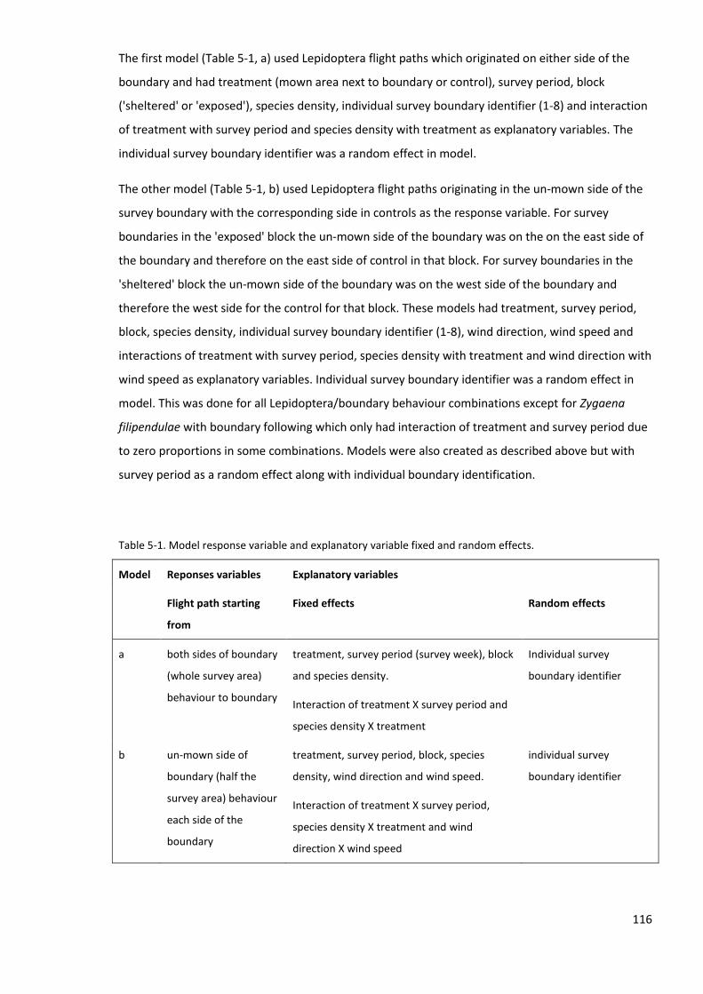
116
The first model (Table 5-1, a) used Lepidoptera flight paths which originated on either side of the
boundary and had treatment (mown area next to boundary or control), survey period, block
('sheltered' or 'exposed'), species density, individual survey boundary identifier (1-8) and interaction
of treatment with survey period and species density with treatment as explanatory variables. The
individual survey boundary identifier was a random effect in model.
The other model (Table 5-1, b) used Lepidoptera flight paths originating in the un-mown side of the
survey boundary with the corresponding side in controls as the response variable. For survey
boundaries in the 'exposed' block the un-mown side of the boundary was on the on the east side of
the boundary and therefore on the east side of control in that block. For survey boundaries in the
'sheltered' block the un-mown side of the boundary was on the west side of the boundary and
therefore the west side for the control for that block. These models had treatment, survey period,
block, species density, individual survey boundary identifier (1-8), wind direction, wind speed and
interactions of treatment with survey period, species density with treatment and wind direction with
wind speed as explanatory variables. Individual survey boundary identifier was a random effect in
model. This was done for all Lepidoptera/boundary behaviour combinations except for Zygaena
filipendulae with boundary following which only had interaction of treatment and survey period due
to zero proportions in some combinations. Models were also created as described above but with
survey period as a random effect along with individual boundary identification.
Table 5-1. Model response variable and explanatory variable fixed and random effects.
Model Reponses variables Explanatory variables
Flight path starting
from
Fixed effects Random effects
a both sides of boundary
(whole survey area)
behaviour to boundary
treatment, survey period (survey week), block
and species density.
Interaction of treatment X survey period and
species density X treatment
Individual survey
boundary identifier
b un-mown side of
boundary (half the
survey area) behaviour
each side of the
boundary
treatment, survey period, block, species
density, wind direction and wind speed.
Interaction of treatment X survey period,
species density X treatment and wind
direction X wind speed
individual survey
boundary identifier

117
5.4 Results
5.4.1 Comparison, a) Lepidoptera between treatment and control survey areas
A total of 389 Lepidoptera were surveyed at control and treatment plots consisting of 148, Maniola
jurtina and 195 Zygaena filipendulae. Of these totals, 159 crossed, 74 followed and 36 avoided
boundaries and 120 stayed within the survey are and therefore no behaviour could be assigned
(Table 5-2).
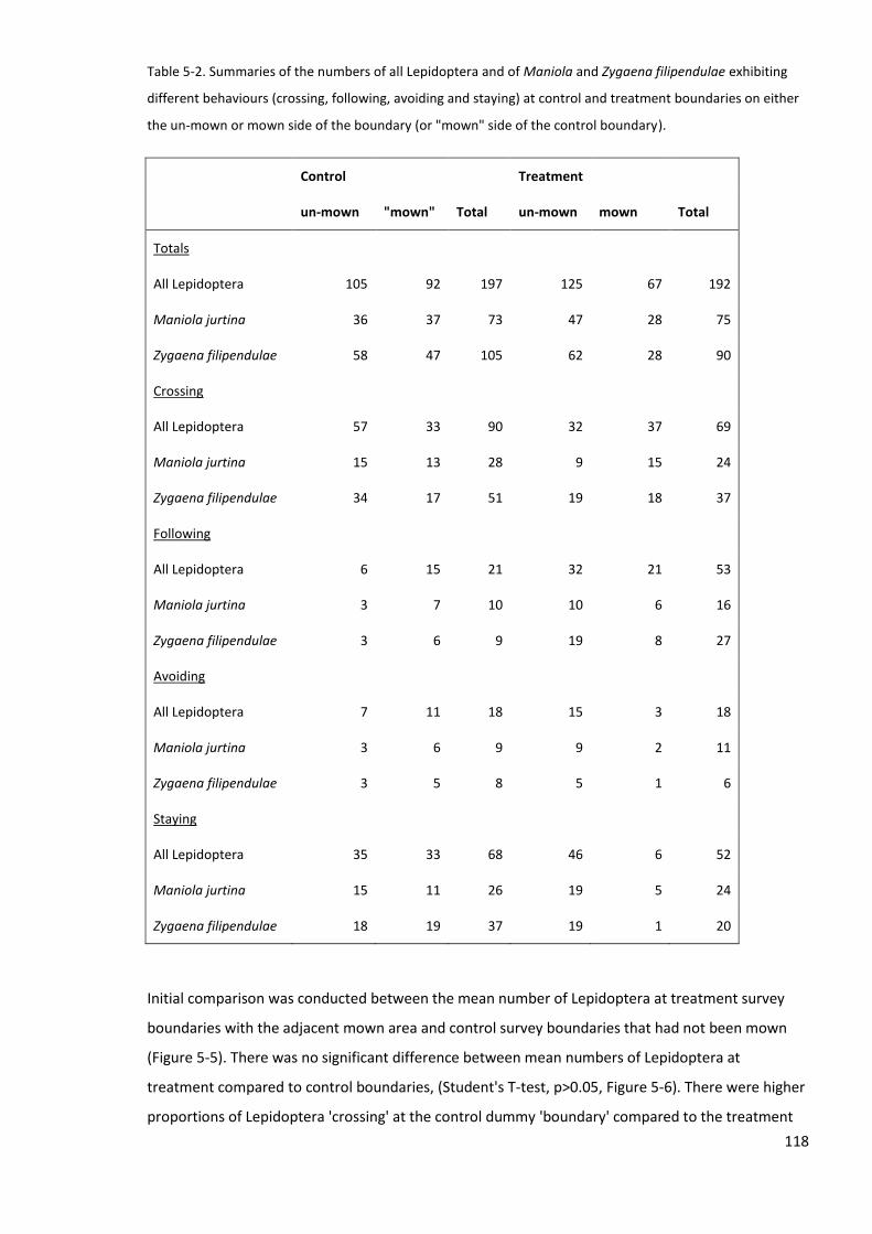
118
Table 5-2. Summaries of the numbers of all Lepidoptera and of Maniola and Zygaena filipendulae exhibiting
different behaviours (crossing, following, avoiding and staying) at control and treatment boundaries on either
the un-mown or mown side of the boundary (or "mown" side of the control boundary).
Control Treatment
un-mown "mown" Total un-mown mown Total
Totals
All Lepidoptera 105 92 197 125 67 192
Maniola jurtina 36 37 73 47 28 75
Zygaena filipendulae 58 47 105 62 28 90
Crossing
All Lepidoptera 57 33 90 32 37 69
Maniola jurtina 15 13 28 9 15 24
Zygaena filipendulae 34 17 51 19 18 37
Following
All Lepidoptera 6 15 21 32 21 53
Maniola jurtina 3 7 10 10 6 16
Zygaena filipendulae 3 6 9 19 8 27
Avoiding
All Lepidoptera 7 11 18 15 3 18
Maniola jurtina 3 6 9 9 2 11
Zygaena filipendulae 3 5 8 5 1 6
Staying
All Lepidoptera 35 33 68 46 6 52
Maniola jurtina 15 11 26 19 5 24
Zygaena filipendulae 18 19 37 19 1 20
Initial comparison was conducted between the mean number of Lepidoptera at treatment survey
boundaries with the adjacent mown area and control survey boundaries that had not been mown
(Figure 5-5). There was no significant difference between mean numbers of Lepidoptera at
treatment compared to control boundaries, (Student's T-test, p>0.05, Figure 5-6). There were higher
proportions of Lepidoptera 'crossing' at the control dummy 'boundary' compared to the treatment

119
boundary (with an adjacent mown area) but the significance was borderline (Figure 5-7 a, X2=3.43,
p=0.0640). There were significantly higher proportions of boundary following at treatment
boundaries for all Lepidoptera and for Zygaena filipendulae compared to expected (Figure 5-5, b, full
results in Appendix D).
Figure 5-5. There were significantly (and borderline) more numbers of all Lepidoptera in total crossing the
control dummy 'boundary' than expected (a) and more following the treatment boundary than expected (b) if
movement was random (p=0.0640 and <0.0001, respectively). There were more Zygaena filipendulae following
the treatment boundary than expected if movement was random (p=0.0003) and no significant difference for
Maniola jurtina.
Figure 5-6. Mean number of all Lepidoptera, Maniola jurtina (Man.jur) and Zygaena filipendulae (Zyg.fil)
between treatment (experimentally mown) boundaries and control boundaries that were not mown. Error
bars show 1 Standard Error of the mean.
0
5
10
15
20
25
All Lepidoptera
Nu
mb
er
of
Lep
ido
pte
ra
(me
an)
Man.jur Zyg.fil
Control
Treatment
a b
(*) ***

120
Figure 5-7. Proportion of, a) Maniola jurtina and Zygaena filipendulae (Man. jur and Zyg. fil respectively),
proportion crossing boundaries for, b) all Lepidoptera p=0.0640, c) Maniola jurtina and, d) Zygaena
filipendulae separately at treatment boundaries (adjacent to mown area) and control boundaries (not mown).
Chi-squared test p>0.05.
0.0
0.2
0.4
0.6
0.8
1.0
Man.jur Zyg.fil
Pro
po
rtio
n o
f Le
pid
op
tera
Treatment
Control
0.0
0.2
0.4
0.6
0.8
1.0
Control Treatment
Pro
po
rtio
n o
f Le
pd
iop
tera
cr
oss
ing
bo
un
dar
y
Other
Cross
0.0
0.2
0.4
0.6
0.8
1.0
Control Treatment
Pro
po
rtio
n o
f M
an
.ju
r cr
oss
ing
bo
un
dar
y
Other
Cross
c
0.0
0.2
0.4
0.6
0.8
1.0
Control Treatment
Pro
po
rtio
n o
f Zy
g.f
il cr
oss
ing
bo
un
dar
y
Other
Cross
a b
d

121
Figure 5-8. Proportion of Lepidoptera following boundaries for, a) all Lepidoptera, b) Maniola jurtina (Man.jur)
and, c) Zygaena filipendulae (Zyg.fil) separately at treatment boundaries (adjacent to mown area) and control
boundaries (not mown). Chi-squared test p<0.0001, 0.3153 and 0.0003, respectively. Significance p<0.001 ***,
p<0.01 **, p<0.05 *.
5.4.2 Comparison, b) Lepidoptera between sheltered and exposed blocks
Comparison was conducted between the mean number of Lepidoptera in the two different blocks to
investigate if the adjacent woodland in the 'sheltered' block affected the distribution and behaviour
of Lepidoptera. There was no significant difference between mean numbers of Lepidoptera in the
two different blocks (more exposed and more sheltered locations, Figure 5-9). There was no
significant difference between proportions of Maniola jurtina and Zygaena filipendulae (Figure 5-10,
a). There were no significant differences between the proportions crossing boundaries for all
Lepidoptera, Maniola jurtina or Zygaena filipendulae separately (Figure 5-10, a) or following
boundaries for Zygaena filipendulae (Figure 5-11,d) and Maniola jurtina following boundaries
between the sheltered and exposed blocks (Figure 5-11, Appendix D for full results).
0.0
0.2
0.4
0.6
0.8
1.0
Control Treatment
Pro
po
rtio
n o
f Le
pid
op
tera
fo
llow
ing
bo
un
dar
y
Other
Follow
0.0
0.2
0.4
0.6
0.8
1.0
Control Treatment
Pro
po
rtio
n o
f M
an
.ju
r fo
llow
ing
bo
un
dar
y
Other
Follow
0.0
0.2
0.4
0.6
0.8
1.0
Control Treatment
Pro
po
rtio
n o
f Zy
g.f
il fo
llow
ing
bo
un
dar
y
Other
Follow
***
a b
c
***

122
Figure 5-9. Mean number of all Lepidoptera, Maniola jurtina (Man. jur) and Zygaena filipendulae (Zyg.fil) at the
exposed and sheltered block. p>0.05. Error bars show 1 Standard Error of the mean.
Figure 5-10. Proportion of, a) Maniola jurtina and Zygaena filipendulae (Man.jur and Zyg.fil respectively),
proportion crossing boundaries for, b) all Lepidoptera, c) Maniola jurtina and, d) Zygaena filipendulae
separately at survey boundaries in more exposed block (Exposed) and more sheltered block (Sheltered)
(includes treatment and control boundary surveys). Chi-squared test p>0.05.
0.00
5.00
10.00
15.00
20.00
25.00
All Lepidoptera
Nu
mb
er
of
Lep
ido
pte
r (m
ean
)
Man.jur Zyg.fil
Sheltered
Exposed
0.0
0.2
0.4
0.6
0.8
1.0
Exposed Sheltered
Pro
po
rtio
n o
f Le
pid
op
tera
Zyg.fil
Man.jur
a
0.0
0.2
0.4
0.6
0.8
1.0
Exposed Sheltered
Pro
po
rtio
n o
f Le
pid
op
tera
cr
oss
ing
bo
un
dar
y
Other
Cross
b
0.0
0.2
0.4
0.6
0.8
1.0
Exposed Sheltered
Pro
po
rtio
n o
f M
an
.ju
r cr
oss
ing
bo
un
dar
y
Other
Cross
c 0.0
0.2
0.4
0.6
0.8
1.0
Exposed Sheltered
Pro
po
rtio
n o
f Zy
g.f
il cr
oss
ing
bo
un
dar
y
Other
Cross
d
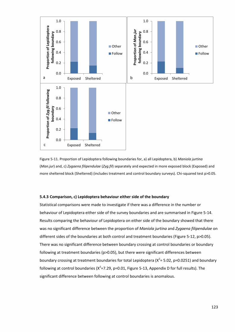
123
Figure 5-11. Proportion of Lepidoptera following boundaries for, a) all Lepidoptera, b) Maniola jurtina
(Man.jur) and, c) Zygaena filipendulae (Zyg.fil) separately and expected in more exposed block (Exposed) and
more sheltered block (Sheltered) (includes treatment and control boundary surveys). Chi-squared test p>0.05.
5.4.3 Comparison, c) Lepidoptera behaviour either side of the boundary
Statistical comparisons were made to investigate if there was a difference in the number or
behaviour of Lepidoptera either side of the survey boundaries and are summarised in Figure 5-14.
Results comparing the behaviour of Lepidoptera on either side of the boundary showed that there
was no significant difference between the proportion of Maniola jurtina and Zygaena filipendulae on
different sides of the boundaries at both control and treatment boundaries (Figure 5-12, p>0.05).
There was no significant difference between boundary crossing at control boundaries or boundary
following at treatment boundaries (p>0.05), but there were significant differences between
boundary crossing at treatment boundaries for total Lepidoptera (X2= 5.02, p=0.0251) and boundary
following at control boundaries (X2=7.29, p=0.01, Figure 5-13, Appendix D for full results). The
significant difference between following at control boundaries is anomalous.
0.0
0.2
0.4
0.6
0.8
1.0
Exposed Sheltered
Pro
po
rtio
n o
f Le
pid
iop
tera
fo
llow
ing
bo
un
dar
y
Other
Follow
a 0.0
0.2
0.4
0.6
0.8
1.0
Exposed Sheltered
Pro
po
rtio
n o
f M
an
.ju
r fo
llow
ing
bo
un
dar
y
Other
Follow
b
0.0
0.2
0.4
0.6
0.8
1.0
Exposed Sheltered
Pro
po
rtio
n o
f Zy
g.f
il fo
llow
ing
bo
un
dar
y
Other
Follow
c

124
Figure 5-12. The proportion of Maniola jurtina and Zygaena filipendulae (Man.jur and Zyg.fil, respectively) in
the un-mown and mown side of the boundary for, a) controls ('Mown' side refers to corresponding side of the
boundary to the treatment but was not mown) and , b) treatments. p>0.05.
Figure 5-13. Proportion of Lepidoptera in the un-mown or mown ('Mown' for control as this was the
corresponding side to the treatment boundary) side of the boundary, a) crossing at control and, b) treatment
boundaries p=0.0251 and, c) following at control p=0.0069 and, d) treatment boundaries. Significance p<0.001
***, p<0.01 **, p<0.05 *.
0.0
0.2
0.4
0.6
0.8
1.0
Un-mown "Mown"
Pro
po
rtio
n o
f Le
pid
op
tera
at
con
tro
l bo
un
dar
ies
Boundary side
Zyg. fil
Man.jur
a
0.0
0.2
0.4
0.6
0.8
1.0
Un-mown Mown
Pro
po
rtio
n o
f Le
pid
op
tera
at
tre
atm
en
t b
ou
nd
arie
s
Boundary side
Zyg. fil
Man.jur
b
0.0
0.2
0.4
0.6
0.8
1.0
Un-mown "Mown"
Pro
po
rtio
n o
f Le
pid
op
tera
cr
oss
ing
con
tro
l bo
un
dar
y
Boundary side
Other
Cross
a
0.0
0.2
0.4
0.6
0.8
1.0
Un-mown Mown
Pro
po
rtio
n o
f Le
pid
op
tera
cr
oss
ing
tre
atm
en
t b
ou
nd
ary
Boundary side
Other
Cross
b
*
0.00
0.20
0.40
0.60
0.80
1.00
Un-mown "Mown"
Pro
po
rtio
n o
f Le
pid
op
tera
fo
llow
ing
con
tro
l bo
un
dar
y
Boundary side
Other
Follow
c
**
0.00
0.20
0.40
0.60
0.80
1.00
Un-mown Mown
Pro
po
rtio
n o
f Le
pid
op
tera
fo
llow
ing
tre
atm
en
t b
ou
nd
ary
Boundary side
Other
Follow
d

125
Figure 5-14. Results showed that there was more Lepidoptera in total crossing the treatment boundary from
the mown side (a, p=0.0251), and more following the dummy 'boundary' from the "mown" side (b, p=0.0069).
5.4.4 Behaviour probability and boundary permeability measures
When comparing the behaviour probabilities, there were no significant differences between the
proportions of Lepidoptera exiting the survey area by crossing the dummy 'boundary' in controls
compared to the expected proportion if survey area exiting behaviour was random (Figure 5-15,
Appendix D for full results). This was based on Lepidoptera flight paths that originated in the un-
mown side of the treatment boundary (with the adjacent mown area) or the corresponding side of
the control boundary. Following the boundary as a survey area exiting behaviour was significantly
lower than expected if behaviour was random at the control boundaries (Figure 5-15) with less than
7% exiting the control survey area by following the dummy 'boundary' in controls (p<0.001).
a b
* **

126
Figure 5-15. The proportion of Lepidoptera (%) exiting the survey area by, a) crossing the boundary and, b)
following the boundary. Results of Chi-squared test comparing this proportion to the 33% that would be
expected if survey area exit behaviour was random (for example, 33% would exit by crossing, 33% by avoiding
and 33% by following the boundary). For all Lepidoptera and for Maniola jurtina and Zygaena filipendulae
separately (Man.jur and Zyg.fil respectively). Significance p<0.001 ***, p<0.01 **, p<0.05 *.
Results from the boundary permeability measure showed that for all Lepidoptera, the proportion
that approached the boundary and then crossed it was similar between treatment and control
boundaries and similar in total for Maniola jurtina. Maniola jurtina, had lower permeability value at
the mown boundaries than the control. Zygaena filipendulae had a higher edge permeability of 70%
(Table 5-3). Overall exiting the survey area through edges perpendicular to the boundary had a lower
permeability but was higher at mown boundaries than controls (Table 5-3).
0
10
20
30
40
50
All lepdioptera Man.jur Zyg.fil
Pro
po
rtio
n o
f Le
pid
op
tera
exi
tin
g p
lot
by
cro
ssin
g th
e b
ou
nd
ary
(%)
Control
Treatment
Linear (Expected)
a
0
10
20
30
40
50
All lepdioptera Man.jur Zyg.fil
Pro
po
rtio
n o
f Le
pid
op
tera
exi
tin
g th
e
plo
t b
y fo
llow
ing
the
bo
un
dar
y (%
)
Control
Treatment
Linear (Expected)
*** *** ***
b
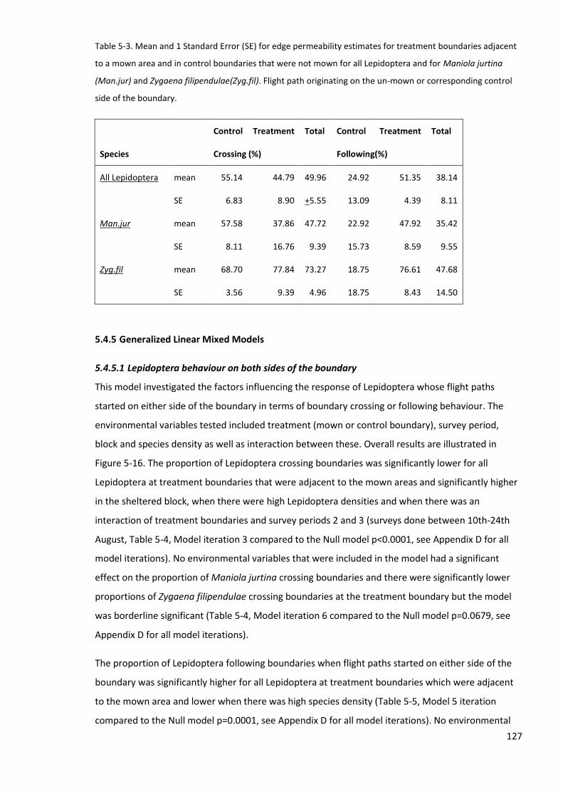
127
Table 5-3. Mean and 1 Standard Error (SE) for edge permeability estimates for treatment boundaries adjacent
to a mown area and in control boundaries that were not mown for all Lepidoptera and for Maniola jurtina
(Man.jur) and Zygaena filipendulae(Zyg.fil). Flight path originating on the un-mown or corresponding control
side of the boundary.
Control Treatment Total Control Treatment Total
Species Crossing (%) Following(%)
All Lepidoptera mean 55.14 44.79 49.96 24.92 51.35 38.14
SE 6.83 8.90 +5.55 13.09 4.39 8.11
Man.jur mean 57.58 37.86 47.72 22.92 47.92 35.42
SE
8.11 16.76 9.39 15.73 8.59 9.55
Zyg.fil mean 68.70 77.84 73.27 18.75 76.61 47.68
SE
3.56 9.39 4.96 18.75 8.43 14.50
5.4.5 Generalized Linear Mixed Models
5.4.5.1 Lepidoptera behaviour on both sides of the boundary
This model investigated the factors influencing the response of Lepidoptera whose flight paths
started on either side of the boundary in terms of boundary crossing or following behaviour. The
environmental variables tested included treatment (mown or control boundary), survey period,
block and species density as well as interaction between these. Overall results are illustrated in
Figure 5-16. The proportion of Lepidoptera crossing boundaries was significantly lower for all
Lepidoptera at treatment boundaries that were adjacent to the mown areas and significantly higher
in the sheltered block, when there were high Lepidoptera densities and when there was an
interaction of treatment boundaries and survey periods 2 and 3 (surveys done between 10th-24th
August, Table 5-4, Model iteration 3 compared to the Null model p<0.0001, see Appendix D for all
model iterations). No environmental variables that were included in the model had a significant
effect on the proportion of Maniola jurtina crossing boundaries and there were significantly lower
proportions of Zygaena filipendulae crossing boundaries at the treatment boundary but the model
was borderline significant (Table 5-4, Model iteration 6 compared to the Null model p=0.0679, see
Appendix D for all model iterations).
The proportion of Lepidoptera following boundaries when flight paths started on either side of the
boundary was significantly higher for all Lepidoptera at treatment boundaries which were adjacent
to the mown area and lower when there was high species density (Table 5-5, Model 5 iteration
compared to the Null model p=0.0001, see Appendix D for all model iterations). No environmental

128
variables in the model were significant for Maniola jurtina and there were higher proportions of
Zygaena filipendulae following at treatment boundaries (Table 5-5, Model 6 iteration compared to
the Null model p=0.0195, see Appendix D for all model iterations).
Figure 5-16. Significantly and borderline significantly lower proportions of all Lepidoptera and Zygaena
filipendulae were crossing (p<0.0001 and p=0.0679, respectively) and significantly higher proportions following
(p=0.0001 and p=0.0195, respectively) at treatment boundaries. There were significantly higher proportions of
Lepidoptera crossing in the sheltered block and when there was a high species density and an interaction of
treatment/control boundary and survey period. There were significantly higher proportions of Lepidoptera
following boundaries when there were lower densities of Lepidoptera.
Table 5-4. Minimum Adequate Model of GLMM for all Lepidoptera, Maniola jurtina (Man. jur) and Zygaena
filipendulae (Zyg. fil) crossing at boundary surveys. Variable estimate (Estimate), Standard error (Std.Error), z
and p value. Significance p<0.001 ***, p<0.01 **, p<0.05 *, 0.1<p>0.05 (*). See Appendix D for all model
iterations. Variables here are treatment or control boundaries, sheltered or exposed block, species density and
survey periods 1,2 or 3.
Crossing Variables Estimate Std.Error z p
All
Lepidoptera
Model iteration 3 compared to Null <0.0001 ***
(Intercept) -1.48 0.77 -1.92 0.0553 (*)
Treatment -1.52 0.42 -3.64 0.0003 ***
Sheltered block 0.57 0.29 1.98 0.0475 *
Total sp. density 0.09 0.02 3.73 0.0002 ***
Control: Survey period 2 -0.48 0.47 -1.03 0.3044
***

129
Treatment: Survey period 2 1.73 0.52 3.36 0.0008 ***
Control: Survey period 3 1.36 0.86 1.58 0.1140
Treatment: Survey period 3 1.29 0.62 2.06 0.0390 *
Man.jur Null
Zyg.fil Model iteration 6 compared to Null 0.0679 (*)
(Intercept) 1.15 0.37 3.09 0.0020 **
Treatment -1.02 0.50 -2.03 0.0428 *
Table 5-5. Minimum Adequate Models of GLMM for all Lepidoptera, Maniola jurtina (Man. jur) and Zygaena
filipendulae (Zyg. fil) following at boundary surveys. Variable estimate (Estimate), Standard error (Std.Error), z
and p value. Significance p<0.001 ***, p<0.01 **, p<0.05 *, 0.1<p>0.05 (*). See Appendix D for all model
iterations. Variables here are treatment or control boundaries and species density.
Follow Variables Estimate Std.Error z p
All
Lepidoptera
Model iteration 5 compared to null 0.0001
(Intercept) -0.33 0.42 -0.77 0.4413
Treatment 1.02 0.30 3.36 0.0008 ***
Total sp. density -0.06 0.02 -3.54 0.0004 ***
Man.jur Null
Zyg.fil Model iteration 6 compared to Null 0.0195 *
(Intercept) -1.92 0.42 -4.59 <0.0001 ***
Treatment 1.44 0.53 2.70 0.0069 **
5.4.5.2 Lepidoptera behaviour on the un-mown side of the boundary
This model investigated the response of Lepidoptera whose flight paths started on the un-mown
side of the treatment boundary or the corresponding control boundary. The behavioural response of
crossing or following behaviour to environmental variables relating to the treatment (mown or
control boundary), survey period, block and species density, wind speed and wind direction as well
as interaction between these. Overall results are illustrated in Figure 5-17. The proportion of
Lepidoptera crossing boundaries was significantly lower for all Lepidoptera for the treatment
boundary which was adjacent to the mown area and significantly higher in the sheltered block (Table
5-6, Model iteration 8 compared to Null model p=0.0003, see Appendix D for all model iterations).

130
There were significantly higher proportions of Maniola jurtina crossing the control boundaries when
there was high species density and significantly lower proportions of Zygaena filipendulae at
treatment boundaries and significantly higher proportions when species density was high and in the
sheltered block (Table 5-6, Model 10 iteration compared to Null model p=0.0099 and model
iteration 7 compared to Null model p=0.0021 respectively, see Appendix D for all model iterations).
The proportion of Lepidoptera following boundaries when flight paths originated from the un-mown
side of the boundary was significantly higher for all Lepidoptera at treatment boundaries and lower
in the sheltered block (Table 5-7, Model 8 iteration compared to Null p=0.0029, see Appendix D for
all model iterations). Increased species density potentially reduced boundary following in Model
iteration 7 which was borderline significantly different in residual deviance to the Minimum
Adequate Model 8 iteration (Table 5-7, Model 7 iteration compared to Null model p=0.0015, X2
Model 7 and Model 8 p=0.0527, see Appendix D for all model iterations). There were significantly
higher proportions of Maniola jurtina following at treatment boundaries and with high wind speed
and lower proportions in survey period 3 (Table 5-7, Model 7 iteration compared to Null model
p=0.0047). There were significantly higher proportions of Zygaena filipendulae following at
treatment boundaries and lower proportions in the sheltered block and when species density was
high (Table 5-7, Model 5 iteration compared to Null model p=0.0002, see Appendix D for all model
iterations).
Figure 5-17. When Lepidoptera flight paths started from the un-mown side of the boundary, there were
significantly lower proportions of all Lepidoptera crossing at treatment boundaries (a, p=0.0004) and higher
proportions crossing in the sheltered block (b, p=0.0137). There was significantly higher proportions of
Lepidoptera following at treatment boundaries (a, p=0.0015) and less in sheltered block and when species
density was low.
b Sheltered block a
***

131
Table 5-6. Minimum Adequate Model for GLMM for all Lepidoptera, Maniola jurtina (Man.jur) and Zygaena
filipendulae (Zyg.fil) crossing the survey boundaries. Variable estimate (Estimate), Standard error (Std.Error), z
and p value. Significance p<0.001 ***, p<0.01 **, p<0.05 *, 0.1<p>0.05 (*). See Appendix D for all model
iterations. Variables here are treatment or control boundaries, sheltered or exposed block and species density.
Crossing Variables Estimate Std.Error z p
All
Lepidoptera
Model iteration 8 compared to Null 0.0004 ***
(Intercept) 1.11 0.33 3.33 0.0009 ***
Treatment -1.94 0.40 -4.89 <0.0001 ***
Sheltered block 0.95 0.39 2.47 0.0137 *
Man.jur Model iteration 10 compared to Null 0.0099 **
(Intercept) -1.68 0.92 -1.82 0.0690 (*)
Control: Man.jur density 0.63 0.26 2.45 0.0145 *
Treatment: Man.jur density 0.14 0.12 1.17 0.2421
Zyg.fil Model iteration 7 compared to Null 0.0021 **
(Intercept) -1.09 0.81 -1.35 0.1782
Sheltered block 1.66 0.58 2.87 0.0042 **
Zyg.fil density 0.28 0.10 2.69 0.0071 **
Zyg.fil density: Treatment -0.27 0.07 -3.73 0.0002 ***

132
Table 5-7. Minimum Adequate Model for GLMM for all Lepidoptera, Maniola jurtina (Man.jur) and Zygaena
filipendulae (Zyg.fil) following the survey boundaries. Variable estimate (Estimate), Standard error (Std.Error), z
and p value. Significance p<0.001 ***, p<0.01 **, p<0.05 *, 0.1<p>0.05 (*). See Appendix D for all model
iterations. Variables here are treatment or control boundaries, sheltered or exposed block, wind speed and
species density.
Following Variables Estimate Std.Error z p
All
Lepidoptera
Model iteration 7 compared to Null 0.0015 **
(Intercept) -1.227 0.61 -2.01 0.0441 *
Treatment 2.14 0.50 4.27 <0.0001 ***
Sheltered block -0.93 0.44 -2.13 0.0334 *
Total sp density -0.06 0.03 -1.93 0.0542 (*)
Model iteration 8 compared to Null 0.0029 **
(Intercept) -2.05 0.45 -4.59 <0.0001 ***
Treatment 2.02 0.49 4.12 <0.0001 ***
Sheltered block -0.84 0.43 -1.98 0.0482 *
Man.jur Model iteration 7 compared to Null 0.0047 **
(Intercept) -7.73 3.02 -2.56 0.0106 *
Treatment 2.67 1.33 2.02 0.0439 *
Survey period 2 1.89 1.14 1.66 0.0964 (*)
Survey period 3 -5.24 2.84 -1.84 0.0653 (*)
Wind speed 0.70 0.34 2.04 0.0417 *
Zyg.fil Model iteration 5 compared to Null 0.0015 **
(Intercept) 0.02 0.96 0.02 0.9807
Treatment 2.64 0.76 3.50 0.0005 ***
Sheltered block -1.47 0.65 -2.24 0.0249 *
Zyg.fil density -0.27 0.11 -2.62 0.0089 **
Overall, the significance of the Minimum Adequate Model when survey period was a random effect
was higher or no different from when survey period was a fixed effect (Appendix D), these results
are in the Appendix D. The environmental variables of treatment boundaries, sheltered block and

133
species density remained significant in the Minimum Adequate Models when survey period was as a
fixed effect and when it was a random effect.
5.4.6 Measures of micro-climate, weather, nectar resources and vegetation characteristics
There was no significant difference in weather or microclimate conditions between the treatment
and control survey areas or between the sheltered and exposed block (p>0.05, Appendix D for table
of results).
As a result of mowing half the survey area, nectar flowers were removed and vegetation density
decreased. Statistical analyses quantified this effect; when comparing the nectar resources and
vegetation characteristics between the treatment and control survey areas, (both sides of the
boundary), there were significantly lower nectar flower numbers (average number of flowering
units, T=5.1069, p<0.0001), in the Fabaceae family (T=3.62, p=0.0015, Figure 5-18) and species
richness (T=2.41, p=0.0254, Figure 5-19) in treatments boundary survey areas. There were also
significantly lower mean and variation in vegetation density (T=6.35, df=12, p<0.0001, Figure 5-19) at
treatment survey area. There were no significant differences between sheltered or exposed blocks.
When comparing nectar resources and vegetation characteristics between the un-mown side of the
boundary and the corresponding control dummy 'boundary' there were borderline significantly
higher species richness (T=1.9504, p=0.0639) but no other differences. There were significantly
higher nectar flowers (average number of nectar flowers T=3.10, p=0.0063), of Yellow Rattle
(Rhinanthus minor, T=2.2664, p=0.0349) and vegetation density (T=4.53, p=0.0002) in the exposed
block (Appendix D for results).
When comparing nectar resources and vegetation characteristics within the treatment survey areas
by comparing between the un-mown and mown sides of the boundary, there were significantly
higher nectar flowers (total number of nectar flowers, T=8.25, p<0,0001, Figure 5-18), Fabaceae
(W=0, df=12, p<0.0001, Figure 5-18) and species richness (W=16, df=12, p=0.0012, Figure 5-19) at
the un-mown side of the boundary. The mown side still provided some nectar flower resources of
low growing and flowering Bird's-foot Trefoil (Lotus corniculatus), Daisy (Bellis perennis) and Black
Medick (Medicago lupulina), whereas the un-mown side had taller flowering plants such as Greater
Knapweed (Centaurea scabiosa), Sainfoin (Onobrychis viciifolia) and Field Scabious (Knautia
arvensis). There were also significantly higher vegetation density and height as measured by the
Drop Disc method Stewart et al. (2001) (T=0.72, df=12, p<0.0001, Figure 5-19) at the un-mown side
of the boundary (There was no significant difference between the un-mown and 'mown' side for
controls, see Appendix D for results).
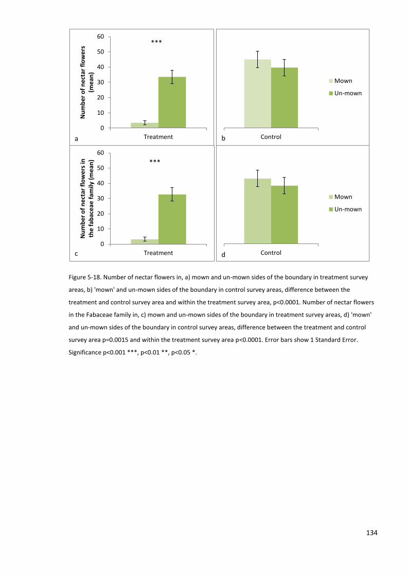
134
Figure 5-18. Number of nectar flowers in, a) mown and un-mown sides of the boundary in treatment survey
areas, b) 'mown' and un-mown sides of the boundary in control survey areas, difference between the
treatment and control survey area and within the treatment survey area, p<0.0001. Number of nectar flowers
in the Fabaceae family in, c) mown and un-mown sides of the boundary in treatment survey areas, d) 'mown'
and un-mown sides of the boundary in control survey areas, difference between the treatment and control
survey area p=0.0015 and within the treatment survey area p<0.0001. Error bars show 1 Standard Error.
Significance p<0.001 ***, p<0.01 **, p<0.05 *.
0
10
20
30
40
50
60
Treatment
Nu
mb
er
of
ne
ctar
flo
we
rs
(me
an)
a
***
Control
Mown
Un-mown
b
0
10
20
30
40
50
60
Treatment
Nu
mb
er
of
ne
ctar
flo
we
rs in
th
e f
abac
eae
fam
ily (
me
an)
c
***
Control
Mown
Un-mown
d

135
Figure 5-19. Nectar flower species richness in, a) mown and un-mown sides of the boundary in treatment
survey areas, b) 'mown' and un-mown sides of the boundary in control survey areas, difference between the
treatment and control survey area p= 0.0254 and within the treatment survey area, p=0.0012. Mean
vegetation density (Drop disc method) in, c) mown and un-mown sides of the boundary in treatment survey
areas, d) 'mown' and un-mown sides of the boundary in control survey areas, difference between the
treatment and control survey area and within the treatment survey area, p<0.0001. Error bars show 1
Standard Error. Significance p<0.001 ***, p<0.01 **, p<0.05 *.
There were a total of 91 Lepidoptera/nectar flower feeding interactions, the majority being from
Zygaena filipendulae and then Maniola jurtina, (52 and 25, respectively). There were a similar
number of Maniola jurtina/nectar flower interactions between the control and treatment survey
areas (13 and 12, respectively) for but more at control than treatment survey areas for Zygaena
filipendulae (40 and 12, respectively). At both controls and treatment survey areas the majority of
Lepidoptera/nectar flower plant interactions were with Greater Knapweed (Centaurea scabiosa, 36
and 12, respectively) then with Field Scabious (Knautia arvensis, 19 and 9, respectively). Lepidoptera
feeding on Red Clover (Trifolium pratense) and Bird's-foot Trefoil (lotus corniculatus) were only
recorded at treatment survey areas. The species which had the highest numbers of
Lepidoptera/nectar flower interactions were Zygaena filipendulae on Centaurea scabiosa, Maniola
0.0
0.5
1.0
1.5
2.0
2.5
3.0
3.5
4.0
Treatment
Ne
ctar
flo
we
r sp
eci
es-
rich
ne
ss
a
**
Control
Mown
Un-mown
b
0
5
10
15
20
25
Treatment
Ve
geta
tio
n d
en
sity
(cm
)
c
***
Control
Mown
Un-mown
d

136
jurtina on Centaurea scabiosa and Zygaena filipendulae on Knautia arvensis (Figure 5-20) which
were not the most abundant nectar flowers within the plots but do produce abundant nectar.
Figure 5-20. The number of Lepidoptera/nectar flower interactions for Maniola jurtina and Zygaena
filipendulae (Man.jur and Zyg. fil respectively). The majority of Lepidoptera/nectar flower interactions being
with Greater Knapweed (Centaurea scabiosa) and Field Scabious (Knautia arvensis).
5.5 Discussion
5.5.1 Lepidoptera response to small scale alterations in habitat structure
Overall, mowing had a weak effect on boundary crossing behaviour as there was no significant
difference between the number of Lepidoptera at survey boundaries or the proportion crossing
boundaries between those survey boundaries adjacent to the mown area and controls (and
compared to expected). However, there were significantly higher proportions of Lepidoptera
crossing from the mown side of the boundary to the un-mown side and vice-versa at treatment
boundaries. Additionally, mowing did affect the proportion of Lepidoptera displaying boundary
following behaviour which was significantly higher for all Lepidoptera and Zygaena filipendulae as
treatment (mowing or control boundary) was a significant variable or interaction term in all
Minimum Adequate Models (except where the Minimum Adequate Model was the null model). This
result is consistent with results in Chapter 4, where a higher proportion of Lepidoptera were
recorded following boundaries at chalk grassland fragments than expected. Boundary following is a
behaviour associated with Lepidoptera in fragmented landscapes (Ovaskainen et al. 2008) and
indicates that uncut areas connected to habitat patches could be utilised by Lepidoptera for
0
5
10
15
20
25
30
Nu
mb
er
of
Lep
ido
pte
ra/n
ect
ar f
low
er
inte
ract
ion
s
Man.jur
Zyg.fil

137
dispersal and are also important refuges for insects that rely on grassland habitat for some part of
their life cycle (Humbert et al. 2012). Boundaries are utilised for navigation during foraging and host-
plant searching to an extent where butterflies will even follow artificial experimental boundaries of
tape and plastic windbreak (Dover & Fry 2001). In fragmented landscapes, some species of
butterflies have increased activity and dispersal but lowered fecundity rates as a trade off (Gibbs &
Van Dyck 2009; Gibbs & Van Dyck 2010) by following habitat edges individuals are increasing the
distance they have to travel to find a more permeable path and this may decrease their fecundity
rates.
This following behaviour indicates that habitat patches that are connected to linear features (for
example, hedgerows, verges and field margins) may be effective to encourage dispersal and increase
landscape connectivity. This management option is supported by studies of Maniola jurtina in
agricultural landscapes where grassy linear features are utilised by many grassland butterfly species
and are important for connectivity and different resources (Delattre et al. 2010b; Ouin et al. 2008).
A habitat patch boundary with an adjacent matrix similar in structure to the habitat increases edge
crossing and dispersal (reviews by Eycott et al. 2012; Prevedello & Vieira 2010). In this study, despite
survey boundaries being within the same grassland re-creation field, the change in vegetation
structure (and the subsequent loss of resources) significantly altered Lepidoptera boundary
behaviour. This is a result similar to an experiment with grasshoppers, in which mown edges were
avoided by grasshoppers even when if they were only mown to half the height of the un-mown
areas (Berggren et al. 2002).
In addition to the mowing treatment, the variables that affected edge crossing behaviour were
block, species density and an interaction of treatment with survey period when flight paths
originated on both sides of the boundary. When considering the boundary behaviour where flight
paths originated on the un-mown side of the boundary, interaction of species density and treatment
was also apparent with lower proportions crossing with high densities at the treatment boundaries
(mown area adjacent) and the opposite for the control boundaries. Species density was a significant
variable explaining both crossing and following behaviours and affects Lepidoptera behaviour in this
study, whereby a high co-specific density can either increase (Ouin et al. 2008) or decrease
(Menendez et al. 2002; Ries & Debinski 2001; Roland et al. 2000) dispersal from habitat patches
depending on the species, sex and habitat characteristics.
Lepidoptera boundary behaviour and the significant environmental variables in Minimum Adequate
Models differed between blocks in sheltered and exposed locations indicating that there may be an
effect of exposure on these behaviours. However, the microclimate conditions that were recorded
did not differ significantly between theses blocks. Block was the significant variable explaining

138
crossing and following behaviours with a lower proportion following and a higher crossing in the
more sheltered block where the habitat to boundary direction was westerly. Wind speed and
direction are likely to interact with shelter by reducing their effects on behaviour, especially when
winds are in a prevailing west and south-westerly direction at the experiment site (as the small
woodland was to the west of the survey boundaries). However, wind direction data was obtained
from the nearest Meteorological station which was located 6 km from the site and so may have not
been accurate. Wind speed and direction can affect the boundary behaviour of Lepidoptera,
increasing boundary crossing when the wind is in that flight direction (Ries & Debinski 2001).
However, the mean microclimate and weather variables did not differ between blocks and a high
wind speed was only significant for Maniola jurtina following boundaries. The effect of shelter and
wind speed on Lepidoptera behaviour is however complex, species specific (Clausen et al. 2001; Ries
& Debinski 2001) and does not always affect butterfly activity (Ovaskainen et al. 2008).
The inclusion of survey period as a fixed or random effect in the models did not affect the overall
variables retained in the Minimum Adequate Models except for when an interaction with treatment
was retained in the Model for all Lepidoptera when flight paths originated from both sides of the
boundary. It may be important to include time as a fixed effect in models due to different emergent
times of butterflies and behaviours that can be affected by interacting temporal, environmental and
intrinsic factors (for example, behaviours relating to mating, feeding or ovipositing). Additionally,
some nectar flower species came into flower soon after they had been mown such as Lotus
corniculatus for example and were then providing some nectar resources in the mown area
(Twiston-Davies, Personal observation). The probability of Lepidoptera crossing habitat patch
boundaries into the matrix can increase over time (Ries & Debinski 2001) as males and females
disperse to locate new mates and to obtain nectar and host plants respectively. However, in this
study the inclusion of survey period as a fixed effect in the Minimum Adequate Model is debatable
given the relatively short survey period in unequal days per survey period.
It is likely that the differences in Lepidoptera responses between treatment and control boundaries
were due to the reduction of nectar resources and vegetation density as a result of the mowing
adjacent to treatment boundaries rather than the physical boundary. This is supported by the results
that showed no significant differences between the numbers or proportions of different behaviours
exhibited in the mown side of the treatment boundary compared to the un-mown side, although
there were lower numbers (5.4.3).
Interpretation of these results is limited by the experimental set up which was restricted by the size
of the experimental area and as a result, survey transects were in relatively close proximity to each
other and with low replication. This low replication of experimental blocks as well as their close
proximity to woodland may confound the results and makes disentangling the effect of shelter on

139
butterfly behaviour difficult as woodland can provide many sources for butterflies that may have not
been measured within the survey areas. However, regarding the microclimate conditions, there
were no significant difference in wind speed, humidity or temperature which may have been as a
result of proximity to shelter. An experiment with more replicated blocks would be recommended
but was not feasible in this study due to the restricted area allocated to setting up the experimental
blocks. Despite this, the high significance values Chi-squared tests and Minimum Adequate Models
especially relating to boundary following behaviour indicate that this experimental set up was
adequate in detecting a behavioural change of Lepidoptera in response to the mowing treatment.
Additionally even though control boundaries were in close proximity to the fence and the woodland,
following behaviour was still significantly higher at the treatment boundaries. Maniola jurtina is
often used as a dispersal indicator species in fragmentation agricultural landscapes and therefore
these results can be transferable to other species especially for those associated with grasslands
(Conradt & Roper 2006; Delattre et al. 2010b) such as Marbled White (Melanargia galathea) and
Ringlet (Aphantopus hyperantus) butterflies for example. However, the low numbers of Lepidoptera
which were dominated by the two focal species may restrict the transferability of these findings due
to species specific responses to and the use of boundaries, habitat patches and habitat structure
(Clausen et al. 2001; Ouin et al. 2004; Ricketts 2001). Total Lepidoptera were comprised
predominantly of Zygaena filipendulae and then Maniola jurtina, although other species responses
were included in the analyses they would have had a low impact on the results. The conservation of
butterfly communities is complex as they are affected by a range of variables (Rosin et al. 2012).
Managing for landscape and habitat patch heterogeneity in vegetation structure, nectar and host-
plant resource and habitat type is advocated (Shreeve & Dennis 2011) as it caters for both the
general and the species specific requirements and behavioural responses.
5.5.1.1 Summary
Mowing has a significant effect on Lepidoptera boundary following behaviour within the same
grassland field by changing the structure and availability of resources and is therefore be an
important management consideration when aiming to increase landscape connectivity. Mowing has
a significant impact on Lepidoptera behaviour, mainly by increasing boundary following behaviour
indicating that more permeable areas and corridors may be an appropriate management option. The
response of Lepidoptera communities is complex, not all species are affected by mowing for
example, Maniola jurtina was not significantly affected and may respond to different management
options so this means that managing for a range of species through habitat heterogeneity (type and
vegetation structure) is important. Boundaries are important sources of resource including dispersal
corridors, nectar sources, oviposition and shelter (Delattre et al. 2010b; Driscoll & Weir 2005; Ouin
et al. 2008), this study investigates the role of boundaries for nectar resources and dispersal and
further studies on the other resources would be recommended.

140
5.5.2 Differences in boundary behaviour between Lepidoptera species
Maniola jurtina did not respond significantly to mown boundaries (for example, Minimum Adequate
Models when flight paths originated on both sides of the boundary) and had lower significance of
Minimum Adequate Models in contrast to Zygaena filipendulae. Additionally, there were differences
in the measures of boundary permeability between species, Zygaena filipendulae had higher
permeability than Maniola jurtina as measured by survey area exiting behaviour compared to
random (44.2% compared to 32.1% respectively) and as the proportion crossing boundaries which
had approached them (at mown boundaries 77.8% and 37.9% respectively). These values for
Maniola jurtina are similar to those reported in (Conradt & Roper 2006) where 25-30% of Maniola
jurtina and Gatekeeper (Pyronia tithonus) crossed boundaries from tall grassland habitat into a
mown short grass matrix. This result suggests that once Zygaena filipendulae are in close proximity
to the boundary they are more likely to cross it and this could be because individuals are responding
to the boundary (following or avoiding) outside of the 20 m by 20 m survey area. This has been
reported in Ries & Debinski (2001) where the more specialist grassland Lepidoptera species Regal
fritillary (Speyeria idalia) avoided edges at 0-20 m whereas the more generalist widespread Monarch
(Danaus plexippus) at 0-9 metres. A lower percentage of Maniola jurtina crossed at boundaries than
controls which reflects results from Chapter 4 where less crossing occurred at chalk grassland
fragments and Maniola jurtina also had a higher proportion avoiding the boundary than Zygaena
filipendulae (Appendix D). These results highlight that even when species utilise the same habitat
they may differ in their response to boundaries and resources (Clausen et al. 2001; Ricketts 2001)
and that a range of boundary behaviours need to be considered to fully understand Lepidoptera
response to habitat boundaries.
Once Zygaena filipendulae reached within 20 m of the edge of the survey area, a higher percentage
crossed than Maniola jurtina at mown boundaries and when compared to controls, and may be
explained by differences in edge sensitivity and dispersal ability of these species. Maniola jurtina has
a higher dispersal ability than Zygaena filipendulae which may related to its edge sensitivity as it will
move on average 50 m-170 m out of habitat patches compared to less than 40 m (with very few over
100 m) for Zygaena filipendulae(Menendez et al. 2002), but is dependent on landscape
characteristics (Ouin et al. 2008). Populations in fragmented landscapes can differ from those from
more continuous landscapes with decreased edge sensitivity and increased activity and flight
distances (Ockinger & Van Dyck 2012; Ovaskainen et al. 2008). Although both species are common in
grasslands, Maniola jurtina is a common species in agricultural landscapes and may therefore be
more adapted to a fragmented landscape of contrasting habitat types and structures.. Additionally,
mowing can harm larvae and pupa (for example, Zygaena filipendulae pupate on long grass stems
which may be damaged if mown early) and therefore a varied mowing and grazing regime

141
throughout the season and within the field may be important to create refuges as demonstrated for
orthoptera in Humbert et al. (2012).
Although there were significant differences in boundary behaviours exhibited by the two study
species, both are associated with grassland habitats. Maniola jurtina is a open-grass associated
species (Shreeve et al. 2001) with larval host plants of Meadow, Bent and Fescue grasses (Poa. sp,
Agrostis. sp and Festuca. sp, respectively) and Zygaena filipendulae is most likely a herb-rich
associated species (Chapter 3) with Lotus corniculatus as its larval host plant, both of which were
present in the grassland recreation field. However, both species are likely to be affected by the
availability of different resources at different scales due to differences in the abundance and
distributions of host plants. For example, Zygaena filipendulae stayed in patches and moved to those
with more host-plants (Menendez et al. 2002) and the presence of a closely related Carniolan burnet
(Zygaena carniolica) was most dependent on nectar plants and the amount of adjacent grassland
habitat (Binzenhofer et al. 2005). This was in contrast to a grass larval host plant species Pearly
Heath (Coenonympha arcania) where larger areas of grassland within 100 m and shrubs and bushes
were important (Binzenhofer et al. 2005).
Limitations of the experimental set up occur from the small study area which can only measure a
section of the entire butterfly flight path and differences in the perceptual ranges of butterflies may
affect the behaviour and the number of individuals entering the survey area. However, as long as the
limitations on interpreting results from this type of experiment are understood, this method
provides the opportunity to investigate these behaviours in a controlled environment setting which
can measure boundary behaviour and edge permeability. Additionally, relatively small experimental
areas have been used to investigate Lepidoptera behaviour to boundaries in other studies for
example, grassland habitat patches 10-40 m wide, survey areas of 40 m by 40 m and grassy field
margins of 10 m and 5 m across (Conradt & Roper 2006; Korpela et al. 2013; Ries & Debinski 2001).
5.5.2.1 Summary
Overall mowing had a significant effect of Lepidoptera boundary behaviours with following
behaviour showing the most significant response. Species-specific responses to boundaries,
variables in the Minimum Adequate Models and in boundary permeability, indicate that
conservation measures designed for more generalist species or for a focal species may not be
appropriate and that these species specific responses need to be considered. Maniola jurtina is
abundant in fragmented agricultural landscapes and potentially not as sensitive to mowing as
Zygaena filipendulae. However, these species may represent other grassland herb rich species that
may significantly alter their behaviour due to mowing and therefore would require management to
mitigate the effect this has on dispersal.

142
Again, these results highlight how boundaries are important sources of dispersal and nectar sources,
however, as well at theses, boundaries are also important for other resources such as providing
suitable microclimate for oviposition and thermoregulation. This study does not investigate these
and therefore further studies on the other resources would be recommended.
5.6 Conclusion
Mowing has a significant effect on Lepidoptera behaviour by increasing boundary following
behaviour, this could be at the cost of other important processes such as fecundity but this result
also suggests that corridors and more permeable areas next to grassland fragments and un-mown
areas may be an effective management options. Species respond differently depending on species-
specific traits relating to foraging and dispersal behaviour and therefore, overall heterogeneous
management at the within field (or habitat patch) and landscape scale is advocated to increase
variation in habitat structure and the resources that are available. Understanding species
behavioural response to grassland management may help to spatially target management and
restoration.

143
Chapter 6 Increased landscape connectivity from a grassland re-creation
scheme at the Stonehenge World Heritage Site, UK
6.1 Introduction
landscape connectivity is important for species in fragmented landscapes (Baguette et al. 2013; Ouin
et al. 2008; Wagner et al. 2013), increasing species viability (Van Teeffelen et al. 2012) and
potentially enhancing ecosystem services (Mitchell et al. 2013).
Evidence-based conservation is essential (Sutherland et al. 2004), however, there is a lack of studies
that translate evidence-based research into policy and explicit management recommendations for
landscape scale projects (Brudvig 2011; Menz et al. 2013; Young et al. 2005). Although it is essential
to recognise that a range of scales are essential for the conservation and restoration of biological
diversity from species and habitats through to landscapes and ecosystems (Lindenmayer et al. 2008).
Landscape connectivity can be enhanced through restoration and conservation focussed actions that
increase the overall size and connectivity of a network of specific habitat patches (Van Teeffelen et
al. 2012). These include a series of measures comprising of the protection of high quality areas,
restoring sites with the most potential, improving the permeability of the matrix between habitat
patches and creating new patches (McIntyre & Hobbs 1999) which form the components of
ecological networks and provide management targets to restore landscape connectivity (Lawton et
al. 2010).
The size of habitat patches in a network and their distance from one another are important
considerations for conservation (Hodgson et al. 2011; Prevedello & Vieira 2010) and the basis for
much of the conservation work based on island biogeography and meta-population theory (Hanski et
al. 1994; MacArthur & Wilson 1967; Moilanen & Hanski 1998). The landscape context and the matrix
land cover between habitat patches can be just as important as they can decrease the functional
distance between habitat patches, thereby increasing functional connectivity (Doerr et al. 2011;
Prugh et al. 2008; Ricketts 2001). There are differences between structural and functional
connectivity in ecology; structural connectivity refers to a network of similar habitat types or
vegetation structure whereas, functional connectivity takes into account the dispersal distances of
the target species or group and the landscape including the intervening matrix between habitat
patches (Tischendorf & Fahrig 2000). Landscape composition is important as it influences the
movement of invertebrates (Delattre et al. 2010b), enhances biodiversity (Vergnes et al. 2012),

144
affects patch characteristics (Ockinger et al. 2012) and supports populations in fragmented
landscapes (Oliver et al. 2010; Steffan-Dewenter & Tscharntke 2002).
In order to provide targeted conservation and evaluate different management, land use and climatic
scenarios, analyses that utilise both habitat patch and matrix characteristics are one of the most
robust methods to measure landscape connectivity. A commonly used method known as cost-
distance analysis is used where the permeability of the intervening matrix between habitat patches
and the dispersal distances of target organisms is included in landscape connectivity evaluation (for
examples see Li et al. 2010; Watts et al. 2010; Watts & Handley 2010). Lepidoptera can be used as
indictors to measure short term changes in restored and re-created grassland, especially chalk
grasslands (Rakosy & Schmitt 2011), and their occurrence in a landscape (indicating biodiversity
improvements as a result of restoration) is likely to result from a combination of patch and
landscape characteristics such as landscape connectivity (Haaland & Bersier 2011; Heer et al. 2013;
Ouin et al. 2008; Thomas et al. 2001b) and an interaction of landscape and habitat quality (Kleijn &
van Langevelde 2006).
The distribution and density of butterflies is affected by their mobility, whereby, more mobile
species are more widely distributed but less densely aggregated (Cowley et al) and they are often
used as a proxy to measure metapopulation dynamics and landscape connectivity for mobile
invertebrates (e.g. Brueckmann et al. 2010; Hanski & Ovaskainen 2000; Ricketts 2001; Severns et al.
2013) . A variety of metrics have been calculated to measure different dispersal abilities, many of
these are estimated using mark and recapture studies and represent emigration rates and
colonisation distances to put butterflies into mobility categories such as Pollard & Yates (1993) and
Bink (1992), others are continuous index value based on questionnaires to experts such as in Cowley
et al. (2001) and Komonen et al. (2004).
Some species with low mobility and specialist larval host plants may not travel over 100 m on
average, for example, the 6-spot Burnet moth (Zygaena filipendulae) and Adonis blue (Lysandra
bellargus) (Menendez et al. 2002; Thomas 1983). However, some specialist species are likely to
travel up to 1000 m and a low number of individuals may even travel 13 km which can maintain
metapopulation dynamics (Baguette 2003). Average dispersal is useful for evaluating landscape
connectivity however, it is important to recognise that these long distance but rare events, can
maintain metapopulation dynamics in fragmented landscapes. The dispersal abilities of a range of
grassland associated but not single host-plant specific butterfly species is potentially between 1-2.5
km including Common Blue (Polyommatus icarus) and Meadow Brown (Maniola jurtina)(Baguette et
al. 2011; Schneider et al. 2003). Maniola jurtina, Ringlet (Aphantopus hyperantus) and Small Heath
(Coenonympha pamphilus) can reach grassy linear features 1 km away from grasslands (Ockinger &
Smith 2007a).

145
The scale at which butterflies are affected by their landscape is also dependent upon mobility and
ecological associations where more specialist butterflies are affected by the landscape composition a
smaller scale (1km buffer) compared to generalist/wider countryside species (5km buffer) Oliver
2010.
The effects of habitat fragmentation on insect interactions are dependent on species and landscape
characteristics (for a review see Tscharntke & Brandl 2004). Therefore, it is important to consider
landscape connectivity for individuals of different taxa and functional groups, with varying species
traits and different habitat associations. This means that the strength and direction of the response
to landscape features and conservation measures can be dependent on these traits, characteristics
and associations and vary between and within species (Keller et al. 2013; Prevedello & Vieira 2010;
Ricketts 2001).
Some semi-natural grasslands have a high biodiversity value (WallisDeVries et al. 2002). However,
species-rich lowland semi-natural grasslands have declined in the UK by 97% since the Second World
War (Fuller 1987) as most improved and semi-natural lowland grasslands were replaced with arable
land during and after the 1940s resulting in high local extinction rates and few grassland
conservation sites remain (Hodgson et al. 2005). A landscape scale grassland restoration and re-
creation project was implemented at the Stonehenge World Heritage Site landscape in Wiltshire, UK,
from 2000-2012. This is situated between large expanses of lowland calcareous grassland and Sites
of Special Scientific Interest (SSSI) across Salisbury Plain, Parsonage Down and Porton Down (Figure
6-1). The site provides an opportunity to investigate the effects of grassland restoration and re-
creation on the connectivity of the landscape scale grassland habitat network.
6.2 Aims and Hypotheses
Aims;
To map and compare the networks of chalk grassland and chalk and neutral grassland
patches before grassland re-creation at the Stonehenge Landscape began in the year 2000
and after the last re-creation field was sown in 2012.
To measure habitat patch and landscape connectivity metrics at two landscape scales; of the
landscape within the World Heritage Site and a 1 km buffer from its boundary and the wider
landscape around the World Heritage Site within an 8 km buffer of its boundary.
To use cost-distance analysis to visualise and evaluate landscape connectivity depending on
the matrix land cover types between grassland patches and the different dispersal abilities
of butterflies.

146
Hypotheses;
i. Landscape scale habitat restoration will increase the area, mean patch size and connectivity
of the grassland network.
ii. The permeability of the matrix land cover will be important in measuring connectivity.
iii. Lepidoptera species with higher mobility will potentially be able to utilise more of the
grassland network compared to those with lower mobility.
iv. Effects of grassland re-creation will be higher at the landscape scale compared to the wider
landscape scale but wider landscape scale effects will be evident.
v. Grassland re-creation will increase the habitat heterogeneity of the landscape.
6.3 Methods and materials
6.3.1 Study Site
The study site was the Stonehenge World Heritage Site (WHS) landscape scale grassland re-creation
project situated between large expanses of lowland calcareous grassland in Wiltshire, UK. Here, over
500 hectares of arable land has been sown with species-rich grassland seed originally sourced from
Salisbury Plain SSSI (Young et al. 2009, Chapter 2, Section 2.1.5, Figure 6-1). This landscape consists
of a grassland network of chalk, neutral, rough and improved grassland types and one of the main
aims of the grassland re-creation scheme was to increase the area of permanent species-rich
grasslands (Young et al. 2009).

147
Figure 6-1. The Stonehenge World Heritage Site and surrounding Sites of Special Scientific Interest (SSSI).
Salisbury Plain, Parsonage Down and Porton Down all large expanses of lowland calcareous grassland.
6.3.2 Land cover mapping
Four separate maps were created to reflect the landscape prior to grassland re-creation in 2000 and
after the last field was sown in 2012. Grassland re-creation was classified into two grassland types,
neutral grassland or chalk grassland, in order to adhere to the broad habitat classification of Land
Cover Maps (Land Cover Map 2007, Morton et al. 2011). Maps were created of: a) the chalk
grassland network in 2000, b) grassland re-creation contributing to the chalk grassland network in
2012, c) chalk and neutral grassland network in 2000 and, d) grassland re-creation contributing to
the chalk and neutral grassland network in 2012.
Land Cover Maps for Wiltshire and Hampshire were sourced from the Centre for Ecology and
Hydrology (Morton et al. 2011). These consisted of broad habitat types at 25 m by 25 m raster grid
square resolution (Land Cover Map 2007). These data were edited in ArcMap (version 10.1 ESRI©) to
reflect the habitat types in 2012 and prior to grassland re-creation in 2000 of the World Heritage Site
based on Stonehenge World Heritage Site management Plans (Young et al. 2009) and personal
observations. Polygons of grassland re-creation in arable fields were classified as either chalk
grassland (maps a and b) or neutral grassland (maps c and d) to investigate the effect of the
Map produced by Grace Twiston-Davies 2014 © Natural England copyright (2014). Contains Ordnance Survey data © Crown
copyright and database right 2014. English Heritage National Monuments Record
148
grassland re-creation on both the chalk grassland network and the chalk and neutral grassland
network (no acid grassland was in the landscape).
Maps of the Lowland Calcareous Grasslands were obtained from Natural England (MAGIC 2014) in
polygon format (data from 1998-2001) and edited to include the additional fragments at the
Stonehenge Landscape on slopes and burial mounds (Winterbourne Stoke Group, Fargo Barrow, Full-
moon Bank and Luxenborough Bank, See Chapter 2, section 2.1). The edited Lowland Calcareous
Grassland map (layer) was combined with the edited Land Cover Maps (layer) for a more accurate
chalk grassland network, as the Land Cover Map classed a larger area as chalk grassland than the
lowland calcareous grassland survey (Natural England, MAGIC 2014) and had excluded small pockets
of chalk grassland. Polygons of Land Cover Map that had been classified as chalk grassland but not
confirmed by the Lowland Calcareous Grassland survey were reclassified as neutral grassland. This
new map was converted to raster at 25 m by 25 m grid square resolution for analysis. The World
Heritage Site boundary was obtained from English Heritage (MAGIC 2014).

149
Figure 6-2. Method for creating grassland habitat network maps using Land Cover Map 2007 and Lowland
Calcareous Grassland map (1998-2001), edited to represent the Stonehenge World Heritage Site (WHS) in
2000 and 2012.
All maps were clipped for editing and analysis using buffers around the Stonehenge World Heritage
Site boundary at 1 km and at 8 km for the Stonehenge Site and the wider landscape habitat
networks, respectively. These scales were chosen as 1km buffer from the WHS boundary included
the chalk grassland on Salisbury plain to the North of the WHS and represented the landscape
context that some specialist species are affect by (Oliver et al. 2010) and the maximum dispersal
Land Cover Map (LCM) 2007 Lowland Calcareous Grassland (LCG) map
Edited to include WHS
grassland re-creation
Edited to include chalk grass
fragments within WHS
Union of LCM and LCG
Classify remaining LCM chalk
grassland as neutral grassland
(b) Chalk grassland
network 2012
Grassland re-creation
classed as chalk grassland
Grassland re-creation classed
as chalk and neutral grassland
network
2000 2012 2012 2000
(a) Chalk grassland
network 2000
(c) Chalk and
neutral grassland
network 2000
(d) Chalk and
neutral grassland
network 2012

150
distances of some specialist butterfly species e.g. approximately 1km (Baguette 2003; Gutierrez
2005; Pe'er et al. 2014). The 8km buffer was selected to include the large expanses of chalk
grassland and SSSIs that surround the WHS an encompass the 5km buffer that wider
countryside/generalist butterflies may be affected by (Oliver et al. 2010) and the scale at which
some long distance dispersal events which maintains metapopulation dynamics e.g. 13km (Baguette
2003). This created a new map to edit without changing the properties of the raw data.
This method only considers land cover changes within the WHS, controlling for land use changes that
may have occurred across the wider landscape (8 km buffer of WHS boundary) between 2000-2012
and enables the landscape-scale effect of the Stonehenge landscape grassland restoration and re-
creation project to be measured and evaluated. This method was used to control for other land-use
changes that may have occurred between 2000 and 2012 in order to evaluate just the grassland
restorations contribution to landscape connectivity and associated habitat patch and landscape
metrics.
6.3.3 Cost-distance analysis
Landscape connectivity was investigated using cost-distance analysis in ArcMap (version 10 ESRI©)
based on the permeability values of different matrix land cover types to a generic focal species
associated with a neutral grassland habitat. These permeability values were calculated using
iterative rounds of expert opinion in a Delphi analysis and displayed as a proportion of relative
permeability for each matrix land cover type with a proportion of 1 being full permeability and 0
being a complete barrier (Eycott et al. 2011, Table 6-1). These values were used on the assumption
that the permeability scores of different matrix land cover types to a neutral grassland associated
species would be similar to that of a chalk grassland associated species. This may overestimate the
connectivity of the landscape as a chalk grassland species may be more sensitive to other land cover
types due to its specialism for short-turf and herb-rich habitats, however, this method provides a
quantitative measure of matrix permeability that can be a basis for evaluating landscape
connectivity. The functional distance between habitat patches can be calculated as the Euclidean
distance between patches divided by the matrix permeability value of the intervening land cover.
For example, if two chalk grassland patches are 50 m apart (Euclidean distance) and are separated
by a matrix of arable land, the permeability of this matrix land cover is 0.05 (Eycott et al. 2011)and
therefore the functional distance between these habitat patches is 1,000 m (50 divided by 0.05,
Figure 6-3). In this example a butterfly in one habitat patch would need to have a dispersal ability of
1,000 m rather than 50 m to reach the other patch due to the low permeability of the intervening
arable land matrix and therefore these two patches would be functionally isolated for those
butterflies with dispersal abilities under 1,000 m.

151
Figure 6-3. Diagram of two chalk grassland habitat patches (1 and 2) separated by a matrix of, a) arable and
horticultural land and, b) Neutral grassland. Permeability value from (Eycott et al. 2011), cost is calculated as 1
divided by the permeability value and functional distance is Euclidean distance divided by the permeability
value or Euclidean distance multiplied by cost. The Euclidean distance between habitat patches 1 and 2 is 50 m
but as the matrix type has either, a) a low permeability value of 0.05 and therefore, the cost of travelling 1m in
the matrix is 20 m and therefore the functional distance is 1,000 m or, b) a high permeability value of 0.575
and therefore, the cost of travelling 1m is 1.74 and the functional distance is 87m.
For cost-distance analysis the permeability value is converted into a 'cost' which is assigned for each
land cover type in the attribute table (ArcMap version 10.1 ESRI©). This is the 'cost' in metres of
travelling 1 metre in the matrix land cover and calculated as 1 divided by the matrix permeability
value (Figure 6-3, Table 6-1). For example, a grassland associated butterfly species may be able to
travel 1,000 m in grassland habitat but will only be able to travel 50 m through a matrix of coniferous
woodland where the permeability value is 0.05 as every 1 metre travelled in this matrix will 'cost' 20
metres (1 divided by 0.05).
From the 'cost' value a separate map (layer) was created (25 m by 25 m grid square resolution) and
this was done for networks of chalk grassland prior to grassland re-creation in 2000, after the last re-
creation field was sown in 2012 and for networks of chalk and neutral grassland in the same years
(maps a-d, Figure 6-5). For the habitat network of chalk grassland all cost values were as described in
(Eycott et al. 2011) except for the cost for a matrix of neutral grassland, which was 1.74 (Table 6-1,
taken from the cost for neutral grassland generic focal species travelling in a matrix of chalk
grassland),the assumption here us that the cost of a chalk grassland matrix to a neutral grassland
species is the same as the cost of a neutral grassland matrix to a chalk grassland species.
Additionally, this method assumes that arable and horticultural land cover have the same cost when
Arable and Horticulture
50 m
1 2
50 m
1 2
Neutral grassland
Euclidean distance =50 m
Functional distance =1,000 m
Euclidean distance = 50 m
Functional distance = 87m
Low permeability (0.05), high 'cost' (20) High permeability (0.575), low 'cost' (1.74)
a b

152
in reality the difference in permeability and resource available in oil-seed rape and winter wheat for
example can be great oil-seed rape can provide early flowering sources of nectar for many nectar
feeding insects (Bartomeus et al. 2014; Riedinger et al. 2014; Woodcock et al. 2013) as well as
microclimate an larval host plants for Pieris. sp. of butterfly (Langmaid et al. 1989).
Table 6-1. Edge impact (metres), permeability value (proportion) and 'cost' of moving 1 metre (1 divided by
permeability value) through different matrix land cover types for a generic focal species associated with
neutral grasslands from (Eycott et al. 2011).
Land cover type Edge impact
(m)
Permeability
value
Cost per
metre
Broadleaved and Yew Woodland 5.0 0.100 10.00
Coniferous Woodland 15.0 0.050 20.00
Arable and Horticulture 10.0 0.050 20.00
Improved Grassland 8.0 0.150 6.67
Neutral Grassland 0.0 0.000 0.00
Calcareous Grassland 0.0 0.575 1.74
Rivers and Streams 4.5 0.050 20.00
Urban/Suburban 10.0 0.075 13.33
Cost-distance is calculated (Spatial Analyst in ArcMap 10.1 ESRI©) as the cumulative Euclidean
distance from a habitat patch multiplied by the cost of each cell it passes (each cell was 25 m by 25
m). The output map represents the habitat network (cost-distance of 0) and the matrix classified by
the functional distance of each part of the matrix and can be interpreted as the dispersal distance an
individual would need to be capable of to reach that matrix patch (Figure 6-4, Figure 6-5).

153
Figure 6-4. Example of focal habitat patch of calcareous grassland and (a) surrounding matrix land cover types
and (b) cost-distance analysis results (calcareous grassland has been overlaid onto the cost-distance map to
highlight patches). Cost-distance is the dispersal distance an individual would need to capable of to reach that
area. For example, all patches are functionally connected to each other for butterflies with dispersal abilities of
up to 1,000 m as they are all within the 0-1,000 m cost-distance categories. Patches B, C and D are all
functionally connected for dispersal abilities up to 250 m as they are separated by high permeability and low
'cost' rough grassland matrix land cover. A butterfly in D would need a dispersal ability of 500-1,000 m to reach
E even though these patches are 260 m away due to the low permeability, high 'cost' Woodland and Improved
pasture matrix.
C
a
b
Maps produced by Grace Twiston-Davies
2013 © Natural England copyright
(2013). Contains Ordnance Survey data
© Crown copyright and database right
2013. LCM2007 © and database right
NERC (CEH) 2011. All rights reserved. ©
third party licensors.
E
E

154
Figure 6-5. Outline of method for Cost-distance analysis in ArcMap (version 10) and interpretation of the
output map.
The assumption of Cost-distance analysis is that travel is linear, however, many studies show that
butterflies may use non-direct but less cost routes such as grassy linear features and tracks (Delattre
et al. 2010b; Ouin et al. 2008) additionally supported in Chapters 4 and 5 in this Thesis. This method
can encompass some of this as it creates a network of last cost areas that are not necessarily direct.
The 25 m by 25 m does means that many linear features are not included. Higher resolution
landscapes can accommodate the inclusion of linear features but this LCM resolution doesn't.
6.3.4 Distribution of focal Lepidoptera species
Distribution data of focal Lepidoptera species from 2000-2012 were obtained from the Butterflies
for the New Millennium Recording Scheme, courtesy for Butterfly Conservation UK and the Wiltshire
and Swindon Biological Records Centre used to investigate the potential role of the grassland re-
creation in linking previously isolated populations. These were presence records of focal species of
conservation concern: Adonis Blue (Lysandra bellargus), Chalkhill Blue (Polyommatus coridon), Small
Blue (Cupido minimus) and the Marsh Fritillary (Euphydryas aurina) which are host plant specialists
New land cover
map (Raster)(a-d)
Cost values for
land cover types
Map based on cost values
for land cover types (Raster)
Focal habitat
network map
(Raster or Ploygon)
Cost-distance analysis
Cost-distance map (Raster) categorises the functional distance of the matrix
Use to interpret functional distance of habitat patches from each other

155
mainly dependent on herb-rich grasslands. Theses presence data were collected by volunteers
reporting random sightings and from surveying regular fixed Butterfly Monitoring Scheme Transects,
there may have been bias in these recordings and areas under represent in survey effort, especially
in the "matrix" land cover where people are unlikely to survey these areas. These data are used to
represent the potential area here these species occur in this landscape but are used with caution.
These species distribution maps were overlaid onto focal grassland networks and the cost-distance
analysis maps for interpretation with the assumption that the distribution across the landscape may
represent populations although most of these presence sights are likely to represent the dispersal of
individuals.
6.3.5 Landscape connectivity measures
Landscape connectivity as a result of the grassland re-creation project was evaluated by calculating
focal habitat patch, network connectivity and landscape-scale measures using Fragstats (version 4.2,
McGarigal et al. 2012). Re-creation grasslands were either classified as adding to the focal chalk
grassland network or adding to the focal chalk and neutral grassland network. The assumption here
is that dispersal is linear rather than indirect but least cost and this data with 25m by 25m resolution
does not accommodate a least cost path using linear features to be measured.
Focal habitat patch characteristic measures were total area of focal habitat (hectares), mean patch
area (hectares) and percentage of the landscape that was focal habitat. The effect of the adjacent
matrix land cover on the focal habitat patch was analysed by measuring the 'core' area and this is
the area of habitat that is left once the edge impacts of the adjacent matrix type have reduced the
habitat area (Figure 6-6). These values were adapted from (Eycott et al. 2011, Table 6-1) to adhere
to the 25 m by 25 m grid square resolution of the data and as a result, adjacent matrix types that
had the highest edge effects of arable land, coniferous woodland and urban/suburban areas were
included as having an edge impact of 25 m (lowest impact that could be used given the resolution of
the data, see Appendix E for this update). The total area of 'core ' focal habitat (hectares), mean
patch core area (hectares) and the percentage of the landscape that was core area were then also
measured (Figure 6-6). Shape index was also calculated, which is based on the perimeter-area ratio
and is a measure of shape complexity, a shape index of 1 is a square patch and the metric value
increases as the patch shape becomes more irregular. Shape index is the simplest measure of shape
complexity and is a good predictor of dispersal success (Calabrese & Fagan 2004; Schumaker 1996).

156
Figure 6-6. Example of how adjacent land cover can reduce the core area of habitat depending on its edge
impact. Here the habitat fragments of chalk grassland are reduced by the edge effect of adjacent land cover of
arable and matrix by 10 m but not affected when the adjacent land cover is neutral grassland. The core area is
reduced. Here four larger patches of chalk grassland in, a) are reduced to six small patches, b) due to the edge
effect of the adjacent matrix.
Connectivity was measured as the Nearest Neighbour Distance and Proximity Index. Nearest
Neighbour Distance is the Euclidean distance to the nearest patch of the same habitat type, this
measures structural connectivity and is used to assess distance to next habitat patch which maybe
important for some low mobility species, this is a widely used and simple measure but does not
necessarily explain patch occupancy as well as some more complex measures (Calabrese & Fagan
2004; Moilanen & Nieminen 2002). Proximity Index, considers the size and proximity of habitat
patches within a specified search radius (based on Gustafson & Parker 1994), these two variables are
important for species conservation (Hodgson et al. 2009; Prevedello & Vieira 2010). The Proximity
Index is zero if there are no other habitat patches of the same type within the search radius.
Proximity Index measures potential connectivity for organisms with the same dispersal abilities of
the search radius and can represent different focal or example species.
Proximity Index measures were based on specific search radiuses of 300 m and 2,500 m to represent
example Lepidoptera with grassland ecological associations based on the dispersal abilities of the 6-
spot Burnet moth (Zygaena filipendulae) and Common Blue (Polyommatus icarus), respectively
(Baguette 2003; Menendez et al. 2002) which are used as examples of focal species by the Forest
Research (Smith et al. 2012). These two species were used as example species as they are in high
abundance in the landscape and colonised older grassland re-creation fields as detailed in Chapter 3,
therefore the connectivity of the landscape may be important for these species. The 6-spot Burnet
a b
Chalk grassland habitat
Neutral grassland, high permeability matrix (no edge impact)
Arable land, low permeability matrix (edge impact 10 m)

157
moth (Zygaena filipendulae) is a sedentary Lepidoptera associated with herb-rich grasslands which
contain its larval host plant Lotus corniculatus in abundance and has a dispersal threshold of 300-500
m ((Heath & Emmet 1985; Menendez et al. 2002). Polyommatus icarus is an intermediate mobility
open-grass associated species with a dispersal distance of approximately 2500 m (Binzenhofer et al.
2005; Pollard & Yates 1993; Shreeve et al. 2001).
Landscape metrics that included all land cover types were calculated as the number of patches and
the total 'core' area, which included the edge impacts of different land cover types to chalk and
neutral grassland as well as coniferous and yew woodland as described in (Eycott et al. 2011)
(coniferous and yew woodland was the other habitat type in the landscape that would have high
edge impact scores from adjacent land cover type and have been calculated by (Eycott et al. 2011),
see Appendix E ). Landscape heterogeneity was also measured as Shannon diversity and evenness,
widely used measure of land-use change (e.g. Antwi et al. 2008; Benini et al. 2010) and landscape
indicators utilised by the European Commission (2014) .
These analyses were conducted for the wider landscape scale (8 km from the WHS boundary) and
the Stonehenge landscape scale (within the WHS and 1 km boundary) for the chalk grassland
network prior to grassland re-creation in 2000 and after the last field was sown in 2012 and similarly
for the chalk and neutral grassland network (relating to maps a-d previously).
6.4 Results
6.4.1 Grassland habitat network and cost distance analysis
Results showed that between 2000-2012, 493 hectares of arable land was converted into grassland,
this is less than the actual recorded amount (Young et al. 2009) due to the 25m by 25m resolution of
the land cover map which has underestimated the area of new re-created grassland. In 2000 chalk
and neutral grassland accounted for 8.8% of the land cover within the WHS and 1km of its boundary,
this was increased by 2013 to 18.27%. In 2000 the majority of land-cover was arable and horticulture
in 2000 at 54.8% followed by improved pasture 18.1%, in 2012 this had been reduced by 9.5% and
chalk and neutral grassland accounted for (Table 6-2).
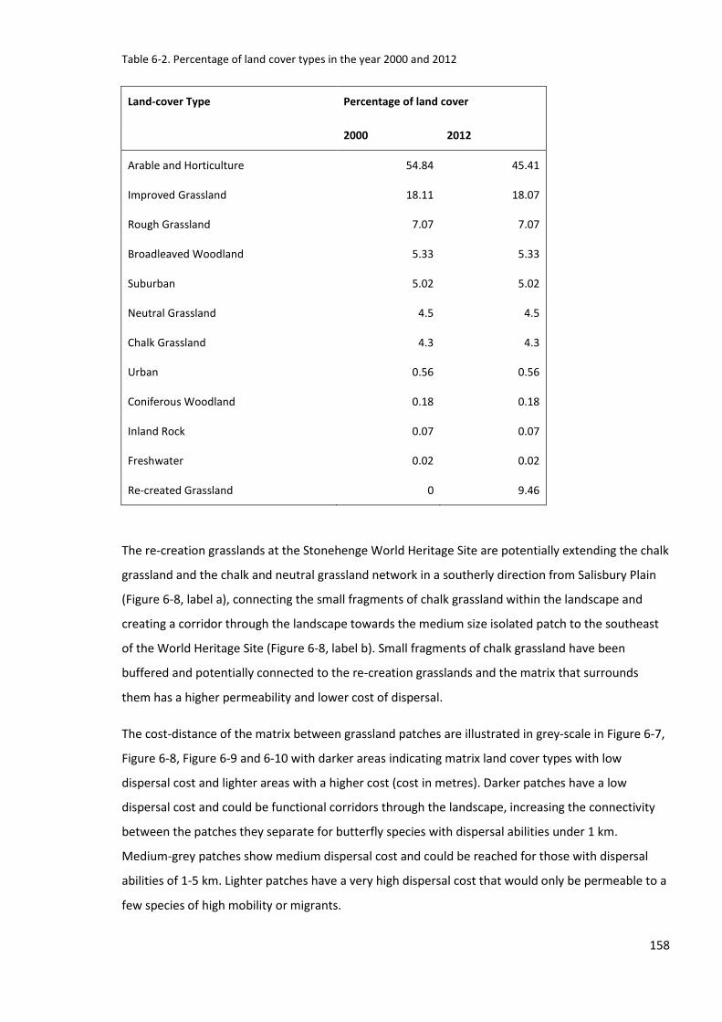
158
Table 6-2. Percentage of land cover types in the year 2000 and 2012
Land-cover Type Percentage of land cover
2000 2012
Arable and Horticulture 54.84 45.41
Improved Grassland 18.11 18.07
Rough Grassland 7.07 7.07
Broadleaved Woodland 5.33 5.33
Suburban 5.02 5.02
Neutral Grassland 4.5 4.5
Chalk Grassland 4.3 4.3
Urban 0.56 0.56
Coniferous Woodland 0.18 0.18
Inland Rock 0.07 0.07
Freshwater 0.02 0.02
Re-created Grassland 0 9.46
The re-creation grasslands at the Stonehenge World Heritage Site are potentially extending the chalk
grassland and the chalk and neutral grassland network in a southerly direction from Salisbury Plain
(Figure 6-8, label a), connecting the small fragments of chalk grassland within the landscape and
creating a corridor through the landscape towards the medium size isolated patch to the southeast
of the World Heritage Site (Figure 6-8, label b). Small fragments of chalk grassland have been
buffered and potentially connected to the re-creation grasslands and the matrix that surrounds
them has a higher permeability and lower cost of dispersal.
The cost-distance of the matrix between grassland patches are illustrated in grey-scale in Figure 6-7,
Figure 6-8, Figure 6-9 and 6-10 with darker areas indicating matrix land cover types with low
dispersal cost and lighter areas with a higher cost (cost in metres). Darker patches have a low
dispersal cost and could be functional corridors through the landscape, increasing the connectivity
between the patches they separate for butterfly species with dispersal abilities under 1 km.
Medium-grey patches show medium dispersal cost and could be reached for those with dispersal
abilities of 1-5 km. Lighter patches have a very high dispersal cost that would only be permeable to a
few species of high mobility or migrants.

159
This has also potentially halved the cost of dispersal in areas adjacent to urban and suburban land
cover that are within the 1 km buffer of the WHS boundary to the East of the World Heritage Site
(Amesbury) that had a very high dispersal cost prior to the grassland re-creation (<20 km dispersal,
Figure 6-8).
The largest expanses of matrix land cover with very high cost are to the east and south-east of the
World Heritage Site. These are urban and suburban areas around the towns of Winterbourne Stoke
and Amesbury/Bulford connected by the A303 road (Figure 6-7 and Figure 6-8, to the West and East
of the WHS respectively). There is also matrix land cover with very high dispersal cost between the
WHS and Porton Down along the A338 road due to these areas being dominated by urban and
arable land cover types (Figure 6-8, Label e).
Within 1 km of the boundary of the WHS, the majority of grassland patches in 2012 (after the
grassland re-creation) are functionally connected for dispersal distances of 1 km-2.5 km except for
the small fragments to the South West of the WHS 1 km buffer. The maximum Lepidoptera dispersal
distance required for patches to be functionally connected has reduced since the grassland re-
creation from 5-10 km in 2000 to 2.5-5 km post re-creation in 2012.

160
Figure 6-7. Map a of the Stonehenge World Heritage Site and the surrounding landscape. Chalk grassland
network and cost-distance matrix in 2000. Cost-distance in metres represents the distance that an individual
would need to be capable of dispersing to reach that area of matrix. Labels, a) Salisbury Plain, b) chalk
grassland patch south-east of the World Heritage Site and, c) Porton Down.
b
c
a
Winterbourne Stoke
Amesbury
Salisbury
Map produced by Grace Twiston-Davies 2013 ©
Natural England copyright (2013). Contains
Ordnance Survey data © Crown copyright and
database right 2013. LCM2007 © and database
right NERC (CEH) 2011. All rights reserved. © third
party licensors. English Heritage National
Monuments Record

161
Figure 6-8. Map b of the Stonehenge World Heritage Site and the surrounding landscape. Chalk grassland
network and cost-distance matrix in 2012. Cost-distance in metres represents the distance that an individual
would need to be capable of dispersing to reach that area of matrix. Labels, a) Sailsbury Plain, b) chalk
grassland patch south-east of the World Heritage Site and, c) Porton Down and, d) isolated fragments.
a
b
c
d
Winterbourne Stoke
Amesbury
Salisbury
Map produced by Grace Twiston-Davies 2013 ©
Natural England copyright (2013). Contains
Ordnance Survey data © Crown copyright and
database right 2013. LCM2007 © and database
right NERC (CEH) 2011. All rights reserved. © third
party licensors. English Heritage National
Monuments Record
e

162
Figure 6-9. Map c of the Stonehenge World Heritage Site and the surrounding landscape. Chalk and neutral
grassland network and cost-distance matrix in 2000. Cost distance in metres represents the distance that an
individual would need to be capable of dispersing to reach that area of matrix. Labels, a) Sailsbury Plain, b)
chalk grassland patch south-east of the World Heritage Site and, c) Porton Down.
a
b
c
Map produced by Grace Twiston-Davies 2013 © Natural
England copyright (2013). Contains Ordnance Survey data ©
Crown copyright and database right 2013. LCM2007 © and
database right NERC (CEH) 2011. All rights reserved. © third
party licensors. English Heritage National Monuments Record

163
Figure 6-10. Map d of the Stonehenge World Heritage Site and the surrounding landscape. Chalk grassland
network and cost-distance matrix in 2012. Cost distance in metres represents the distance that an individual
would need to be capable of dispersing to reach that area of matrix. Labels, a) Sailsbury Plain, b) chalk
grassland patch south-east of the World Heritage Site and, (c) Porton Down and (d) isolated fragments.
a
b
c
d
Map produced by Grace Twiston-Davies 2013 © Natural
England copyright (2013). Contains Ordnance Survey data ©
Crown copyright and database right 2013. LCM2007 © and
database right NERC (CEH) 2011. All rights reserved. © third
party licensors. English Heritage National Monuments Record

164
6.4.2 Distribution of focal Lepidoptera species
Distribution maps of focal Lepidoptera species from the Butterflies for the New Millennium
Recording Scheme along with the recording of Lepidoptera from this study (Chapters 3, 4 and 5 not
shown in the Figure) indicate that the Stonehenge grassland re-creation has the potential to connect
populations of Lysandra bellargus and Cupido minimus within the Stonehenge Landscape to each
other and to link these populations to those in Salisbury Plain to the north of the site (Figure 6-10).
Euphydryas aurinia have been recorded across Salisbury Plain but not at the Stonehenge WHS and
therefore the grassland re-creation may only enhance the connectivity of the landscape by
decreasing the dispersal 'cost' and not necessarily link potentially isolated populations (see Appendix
E for map with Euphydryas aurinia distributions). There have been many recordings of Lysandra
bellargus and Cupido minimus in the low permeability, high 'cost' suburban matrix area of Amesbury
to the East of the WHS boundary (Figure 6-10), from 2000-2012; these are from the Boscombe Down
Butterfly Monitoring Transect on an area that is classed as improved grassland.

165
Table 6-3. Adonis Blue (Lysandra bellargus) and Small Blue (Cupido minimus) and Chalkhill Blue (Polyommatus
coridon) sightings in the Stonehenge World Heritage Site and 1 km buffer. Map location on Figure 6-11.
Appendix E for all species distributions of interest.
Species No.
seen
Month Year Location Map location Fixed
transect
Adonis Blue 4 May, June 2010 Salisbury Plain a
Adonis Blue 1 June 2010 Salisbury Plain a
Adonis Blue 11 September 2011 Salisbury Plain a
Adonis Blue 1 None 2011 Salisbury Plain a
Adonis Blue 4 June,
September
2010 Larkhill Garrison b
Adonis Blue 4 None 2011 Larkhill Garrison b
Adonis Blue 3 August 2004 Fargo Barrow c
Adonis Blue 3 June 2012 Cursus Barrows d
Adonis Blue 3 June 2006 Great Durnford, Little Down
East
f
Small Blue 1 June 2009 Salisbury Plain a
Small Blue 1 June 2009 Salisbury Plain a
Small Blue 1 July 2010 Salisbury Plain a
Small Blue >100 May, June,
July,
August
2010 Larkhill Garrison b
Small Blue 39 None 2011 Larkhill Garrison b
Small Blue 4 None 2010 Normanton Down e
Small Blue 4 None 2010 Normanton Down e RSPB
transect
Chalkhill
Blue
1 None 2006 Normanton Down e RSPB
transect
Chalkhill
Blue
1 None 2007 Normanton Down e RSPB
transect

166
Figure 6-11. Map of the Stonehenge World Heritage Site and the surrounding landscape with locations of
sightings of Adonis Blue (Lysandra bellargus) and Chalkhill Blue (Polyommatus coridon) from 1999-2012. Chalk
and neutral grassland network and cost-distance matrix in 2012. Cost-distance in metres represents the
distance that an individual would need to be capable of dispersing to reach that area of matrix. Labels refer to
a
c
d
e
f
b
Amesbury recordings
Map produced by Grace Twiston-Davies 2013 © Natural England copyright
(2013). Contains Ordnance Survey data © Crown copyright and database right
2013. LCM2007 © and database right NERC (CEH) 2011. All rights reserved. ©
third party licensors. English Heritage National Monuments Record.

167
sightings at, a) Salisbury Plain, b) Larkhill Garrison, c) Fargo Barrow, d) Cursus Barrows, e) Great Durnford, Little
Down East and, f) Normanton Down RSPB reserve. Recordings in the town of Amsbury area are also
highlighted. Lepidoptera distribution data were provided from the Butterflies for the New Millennium
Recording Scheme, courtesy of Butterfly Conservation.
6.4.3 Landscape connectivity measures
At the wider landscape scale, the grassland re-creation at the Stonehenge WHS has had a small but
measurable effect by increasing the number of chalk and neutral grassland patches over4 hectares
from 30 to 38 patches which is the Minimum Area Requirement (MAR) for habitat for the minimum
viable population size of many grassland associated butterfly species such as Aphantopus
hyperantus, Coenonympha pamphilus, Polyommatus icarus, Cupido minimus (MAR 1 ha), Arica
agestis, Lycaena phlaeas and Melanargia galathea (MAR 4 ha) (Bink 1992). The grassland re-
creation has also increased the mean area of a grassland patch by over 1.5 hectares (see Appendix E
for full table of results). Within the WHS and a 1 km boundary as a result of the grassland re-creation
project, the total number of habitat patches and number of patches over 2 hectares in area (Figure
6-12) have increased. This is true also of the total area of grassland and mean area of a patch of
grassland (Figure 6-14) which has increased to 19 and 23 ha for chalk and neutral and for chalk
grassland respectively, now potentially encompassing the MAR of Maniola jurtina and Lysandra
bellargus (16 ha) for example and the percentage of the landscape that are grassland patches that
have increased (Figure 6-13).
The total area, mean patch area and percentage of the landscape of core grassland also increased
after re-creation across the wider landscape and within the WHS (Figure 6-13), this is the amount of
grassland patch that remains once the edge impact (metres) of the adjacent matrix type has been
removed (refer to section 6.3.5 for details on how core area was calculated). This was lower than the
total amount of grassland that was re-created due to the edge impacts of the surrounding matrix
land cover types within the World Heritage Site of predominantly arable land.
The complexity of grassland patches as measured by the Shape index, (similar to perimeter area
ratio) increased due to the irregular shape of the grassland re-creation.
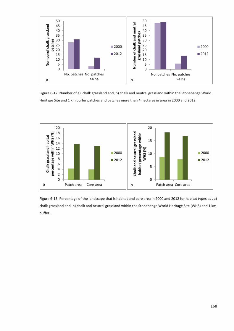
168
Figure 6-12. Number of a), chalk grassland and, b) chalk and neutral grassland within the Stonehenge World
Heritage Site and 1 km buffer patches and patches more than 4 hectares in area in 2000 and 2012.
Figure 6-13. Percentage of the landscape that is habitat and core area in 2000 and 2012 for habitat types as , a)
chalk grassland and, b) chalk and neutral grassland within the Stonehenge World Heritage Site (WHS) and 1 km
buffer.
0 5
10 15 20 25 30 35 40 45 50
No. patches No. patches >4 ha
Nu
mb
ero
f ch
alk
gras
slan
d
pat
che
s
2000
2012
0 5
10 15 20 25 30 35 40 45 50
No. patches No. patches >4 ha
Nu
mb
er
of
chal
k an
d n
eu
tral
gr
assl
and
pat
che
s
2000
2012
0
2
4
6
8
10
12
14
16
18
20
Patch area Core area
Ch
alk
gras
slan
d h
abit
at
pe
rce
nta
ge w
ith
in W
HS
(%)
2000
2012
a 0
5
10
15
20
Patch area Core area
Ch
alk
and
ne
utr
al g
rass
lan
d
hab
itat
pe
rce
nta
ge w
ith
in
WH
S (%
)
2000
2012
b
a b

169
Figure 6-14. Area (hectares) of, a) Chalk grassland and, b) Chalk and neutral grassland within the Stonehenge
World Heritage Site (WHS) and 1 km buffer and percentage of core chalk grassland/chalk and neutral grassland
once the edge effects of the adjacent matrix were considered in 2000 and 2012.
Measures of network connectivity included the distance in metres to the nearest habitat patch using
Nearest Neighbour Distance, which decreased across the wider landscape by 10 m and within the
WHS by 100 m (Figure 6-15). The Proximity Index increased for both dispersal distances and wider
landscape and within the WHS and 1 km buffer (Figure 6-16).
Results from landscape metrics that consider all types of land cover and not just focal habitats of
chalk and neutral grassland showed that the number of patches of different land-cover types
increased across the wider landscape and within the WHS and its 1 km buffer as large expanses of
arable land were broken up by grassland re-creation. Grassland re-creation also increased the total
amount of 'core' area by 18.9 and 19.5 hectares (for wider landscape and WHS scales, respectively
see Table 6-4) as grassland has a much lower edge impact on coniferous and yew woodlands
compared to arable land. There were small but measurable increases in landscape heterogeneity
calculated by diversity and evenness that were more pronounced within the WHS and its 1 km
boundary (Table 6-4, see Appendix E for full results table).
0
5
10
15
20
25
Patch area (mean)
Core area (mean)
Ch
alk
gras
slan
d h
abit
at w
ith
in
WH
S (H
a)
2000
2012
a
0
5
10
15
20
25
Patch area (mean)
Core area (mean)
Ch
alk
and
ne
utr
al g
rass
lan
d
hab
itat
wit
hin
WH
S (H
a)
2000
2012
b

170
Table 6-4. Results from landscape metric calculations considering all habitat patch types of re-creation
grasslands contributing to the chalk grassland network and to the chalk and neutral grassland network.
Measured at the scale of the surrounding landscape in N 8 km buffer from the World Heritage Site boundary
(Surrounding landscape 8 km buffer) that encompasses the many other large expanses of chalk grassland and
within the 1 km buffer of the World Heritage Site (Stonehenge landscape 1 km buffer). Values in 2000 before
the re-creation project started, after 2012 when it was finished and the difference.
Surrounding landscape (8km
buffer)
Stonehenge Landscape (1km
buffer)
Metric 2000 2012 Change 2000 2012 Change
Landscape
Total core area (Ha) 36672.50 36691.38 18.88 4679.94 4699.44 19.50
Re-creation grasslands adding to chalk grassland network
Number of patches 3398.00 3404.00 6.00 444.00 451.00 7.00
Shannon diversity 1.67 1.68 0.01 1.46 1.62 0.17
Shannon evenness 0.65 0.65 0.00 0.61 0.68 0.07
Re-creation grasslands adding to chalk and neutral grassland network
Number of patches 2605.00 2610.00 5.00 387.00 392.00 5.00
Shannon diversity 1.49 1.49 0.01 1.39 1.52 0.13
Shannon evenness 0.60 0.60 0.00 0.61 0.66 0.05
Figure 6-15. Nearest Neighbour Distance (Euclidean distance in metres) for habitat patches of, a) chalk
grassland and, b) chalk and neutral grassland within the Stonehenge World Heritage Site (WHS) and 1 km
buffer in 2000 and 2012.
0
50
100
150
200
250
300
350
Nearest Neighbour Distance
Ch
alk
gras
slan
d N
ear
est
N
eig
hb
ou
r D
ista
nce
wit
hin
W
HS
(m)
2000
2012
a
0
50
100
150
200
250
300
350
Nearest Neighbour Distance
Ch
alk
and
ne
utr
al g
rass
lan
d
Ne
are
st N
eig
hb
ou
r D
ista
nce
w
ith
in W
HS
(m)
2000
2012
b

171
Figure 6-16. Proximity Index of 2,500 m and 300 m threshold to represent potential dispersal distance for
Zygaena filipendulae and Polyommatus icarus as example species for habitat networks of, a) chalk grassland
and, b) chalk and neutral grassland within the Stonehenge World Heritage Site and its 1 km buffer in 2000 and
2012.
6.5 Discussion
6.5.1 Habitat network and cost-distance analysis
Focal habitat networks and cost-distance analysis show that the grassland re-creation project within
the Stonehenge World Heritage Site has increased the area and extent of species-rich grassland
South from Salisbury Plain, into an area that was predominantly arable land and semi-improved
pasture (Figure 6-8, 6-10). This has also potentially halved the cost of dispersal (Section 6.4.1) in
areas adjacent to urban and suburban land cover that are within the 1 km buffer of the WHS
boundary to the East of the World Heritage Site (Amesbury) that had a very high dispersal cost prior
to the grassland re-creation (<20 km dispersal, Figure 6-8). The grassland re-creation has potentially
reduced the Lepidoptera dispersal ability required for functional connectivity between the majority
of grassland patches within the WHS from 5 to 10 km (Figure 6-7, Figure 6-9) to 1 to 2.5 km.
Functional connectivity for the majority of grassland fragments for species with dispersal abilities of
1-2.5 km reflects the upper range of mean dispersal abilities of a range of grassland associated
butterfly species including Common Blue (Polyommatus icarus) and Meadow Brown (Maniola
jurtina)(Baguette et al. 2011; Schneider et al. 2003). Maniola jurtina, Ringlet (Aphantopus
hyperantus) and Small Heath (Coenonympha pamphilus) can reach grassy linear features 1 km away
from grasslands (Ockinger & Smith 2007a). Maniola jurtina will move on average up to 350 m in
short grassland (Conradt & Roper 2006), indicating a dispersal ability of approximately 2333m if the
permeability of this matrix land-cover types is 0.15 (350 divided by 0.15, Eycott et al. 2011).
0
20
40
60
80
100
120
140
160
180
2500m Threshold
300m Threshold
Ch
alk
gras
slan
d p
atch
P
roxi
mit
y In
de
x (m
)
2000
2012
a
0
20
40
60
80
100
120
140
160
180
2500m Threshold
300m Threshold
Ch
alk
and
ne
utr
al g
rass
lan
d
pat
ch P
roxi
mit
y In
de
x (m
)
2000
2012
b

172
Limitations to the enhancement of landscape connectivity as a result of the grassland re-creation are
due to the small fragments of chalk grassland South of the World Heritage Site (Figure 6-8, label d)
that may still remain functionally isolated in the absence of targeted conservation actions and these
are isolated from the re-creation grasslands for species with dispersal abilities under 2.5 km.
Additionally, the grassland network between Salisbury Plain to the North, Parsonage Down to the
West and Porton Down to the east of the WHS may still remain mainly functionally isolated from one
another for all but very high distance dispersers (10-20 km dispersal distances only likely for migrant
species such as the Painted Lady (Vanessa atalanta) or a very few individuals of widespread species)
due to low permeability and high dispersal cost of the arable land between Parsonage Down and
Stonehenge WHS and between Stonehenge WHS and Porton Down. This large landscape scale
perspective is important when considering meta-population dynamics and the future persistence of
populations in the landscape (Hanski 1998; Hanski et al. 1994). However, large landscape scale
projects to increase connectivity of habitat networks can be difficult due to complications and
conflicts arising from the need to reconcile different land owner objectives and arable, residential
and conservation priorities.
Although the majority of fragments are functionally connected for Lepidoptera with dispersal
abilities of 1-2.5 km, many grassland specialist species may still be functionally isolated due to the
high 'cost' of travelling through the matrix and low dispersal abilities. For example Lysandra
bellargus butterflies may not travel any more than 100 m from their residential patch (Thomas 1983)
which means that if habitat patches in close proximity but are separated by a high cost matrix,
individuals may be potentially isolated. In addition to this the fact that male and female dispersal can
differ as dispersal can be affected by different environmental and population factors and can differ
in dispersal distances (Matter & Roland 2002; Rusterholz & Erhardt 2000; Schultz et al. 2012) which
then skews the sex ratio within populations and the differences between sexes have not been
investigated.
In urban and suburban areas, which have very low permeability and high dispersal 'cost' other
policies may need to be considered. However, in landscapes dominated by agricultural land, gardens
can enhance the abundance and richness of pollinators for example by providing floral resources not
otherwise found in the landscape (Samnegard et al. 2011) and therefore, not all urban and suburban
areas necessarily have a high "cost". These could include targeting for urban biodiversity or Agri-
environment schemes that prioritise species-rich grasslands to increase connectivity through these
landscapes for example, Amesbury, arable land west of the Stonehenge Landscape and the Salisbury
City area (Figure 6-8).
The assumption of the grassland re-creation adding to the chalk grassland network is made on the
transitional mesotrophic and chalk botanical characteristics of re-creation grasslands over 7 years

173
old (Campbell 2009; Pemberton 2011; Twiston-Davies et al. in press) and assumes that Lepidoptera
with chalk grassland habitat associations would be able to fully utilise this new network. This time
threshold is supported by studies for other grasslands sown with locally sourced seed mixtures
(Prach et al. 2013), for butterfly communities in re-creation grasslands (Woodcock et al. 2012a) and
for mobile invertebrate species that are characteristic of the target habitat which can re-colonise
grasslands in as little as 2 years (Deri et al. 2011). This however, may not be the case if the larval host
plants of Lepidoptera are not well established across the landscape, for example, Horseshoe Vetch
(Hippocrepis comosa) for Lysandra bellargus. However, given that 7-10 years after first sowing, the
grasslands are approaching the botanical conditions of the target chalk grassland on Salisbury Plain
(Chapter 3 and (Twiston-Davies et al. in press), the assumption that the grassland re-creation can
contribute to the chalk grassland network may be true in the future given time and specific
management. Results from Chapter 3 suggest that re-created grasslands that are over 7 years since
sowing contribute to the chalk grassland network and those that are younger, which have
transitional grassland characteristics contribute to the chalk and neutral grassland network, this
means that this grassland network represents the future potential of the landscape to support chalk
grassland and its associated Lepidoptera species.
The contribution of re-creation grasslands to the chalk and neutral grassland network may be more
realistic given the transitioned botanical conditions and therefore less specialised grassland species
may utilise this new habitat such as Marbled White (Melanargia galathea), Polyommatus icarus and
6-spot Burnet moth (Zygaena filipendulae) with larval host plants highly abundant in the re-creation
grasslands (Campbell 2009; Pemberton 2011). Many species associated with chalk grassland in
Europe are also found in other types of species-rich grasslands and are abundant across the
Stonehenge landscape such as Polyommatus icarus, Melanargia galathea and Coenonympha
pamphilus (Chapter 3) and these are most likely to benefit from the grassland re-creation (van Swaay
2002). Most species surveyed in the re-creation fields were associated with open-grass grasslands
such as Melanargia galathea, Maniola jurtina and Coenonympha pamphilus, (Shreeve et al. 2001)
and therefore the contribution of the re-creation grasslands to the chalk and neutral network is
more realistic at present.
Habitat network and cost-distance maps can inform strategic conservation and management but do
have limitations. Habitat can be defined in many ways; butterflies have overall habitat associations
but these may be wide and flexible depending on species, location (range) climatic and population
factors. Habitat preferences are based only on a single habitat type, and many butterflies have
supplementary and complementary resources or require particular habitat types for shelter in the
matrix (Clausen et al. 2001; Rosin et al. 2012) and habitat affinity can better explain biodiversity as
this considers a multiple habitat types rather than just one habitat type (Proença & Pereira 2013).

174
Additionally, the effects of different matrix types are species specific with even closely related
species responding differently (Prevedello & Vieira 2010; Ricketts 2001; Ries & Debinski 2001).
Linear features in the landscape such as hedgerows, lanes, verges and grassy field margins are
important for invertebrate colonisation, dispersal, growth, survival and species-richness and
abundance (Berggren et al. 2001; Clausen et al. 2001; Delattre et al. 2013; Driscoll & Weir 2005;
Duelli & Obrist 2003; Ockinger & Smith 2007b). The 25 m by 25 m grid square resolution however
does not accommodate these features.
6.5.1.1 Summary
Habitat network properties such as the total area of habitat and connectivity are important for
species persistence (review see Van Teeffelen et al. 2012) and overall the grassland re-creation
project has increased the area of permanent species-rich grassland and reduced the dispersal 'cost'
of the matrix within the 1 km buffer of the WHS. However, this network may be only functionally
connected for species with dispersal abilities of over 1 km, meaning that those of lower dispersal
abilities may be functionally isolated in some patches and therefore will require targeted
conservation action. These types of analysis are useful for targeting area which are most suited for
restoration such as through opportunity mapping, and this is recommended for future projects.
6.5.2 Lepidoptera distribution
Focal Lepidoptera species distribution maps indicate that the grassland network has the potential to
link populations of Lepidoptera that may have previously been functionally isolated due to the low
permeability, high dispersal 'cost' land cover types, between habitat patches within the Stonehenge
World Heritage Site of arable land and semi-improved pasture. Within the landscape, Lysandra
bellargus butterflies were surveyed at a few of the chalk grassland fragments (Chapter 3) and Cupido
minimus at one chalk grassland fragment. These species have specific host plant requirements and
very low mobility so are likely to benefit from grassland re-creation through the effect of buffering of
their chalk grassland fragments, which increases the availability of resources and potentially
increases connectivity.
Limitations of classifying the re-creation grasslands as either chalk or neutral grassland occur due to
the transitional habitat type of the grassland re-creation. Even though older re-creation shares many
similar species with the chalk grassland target habitat patch from where the seed was sourced
(Chapter 3), it can take decades for grassland re-creation to reach the precise botanical conditions of
the target habitat (Fagan et al. 2008). This leaves the classification of grassland re-creation and
interaction networks difficult and potentially designated as sub-optimal habitat or matrix
enhancement depending on the age and floristic composition. Despite these limitations, even a
matrix of similar structure increases dispersal (see for reviews (Eycott et al. 2012; Prevedello & Vieira

175
2010). For the purposes of this study the grassland re-creation was classified as either adding to the
chalk grassland network due to its species-rich characteristics and dominant plant species associated
with chalk grassland (for example, Upright Brome, Bromopsis erecta and Quaking Grass, Brizia
media), or as adding to the more general chalk grassland and neutral grassland network. However,
grassland re-creation would be more beneficial for grassland Lepidoptera species than arable land or
improved pastures as it is less intensively managed and more species-rich, thereby providing
additional resources such as, nectar flower abundance and diversity, which are important for
supporting Lepidoptera abundance and species-richness (Binzenhofer et al. 2005; Clausen et al.
2001; Haaland & Bersier 2011; Matter & Roland 2002). Grassland re-creation can protect and buffer
species-rich grassland fragments that are sources of more specialised butterfly species such as
Lysandra bellargus and Cupido minimus and provide low dispersal 'cost' links through the landscape
to aid dispersal. Additionally, the recordings of Lysandra bellargus and Cupido minimus in improved
grassland at Boscombe Down indicate that an area not classified as 'habitat' using LCM classifications
may be important for supporting these populations.
6.5.2.1 Summary
Grassland re-creation can protect and buffer fragmented patches of chalk grassland, providing
nectar resources and a more permeable matrix land cover for more specialist species even if their
larval host plant require chalk grassland preferences for. However, some species of conservation
concern may still remain functionally isolated if the dispersal 'cost' of travelling through the matrix is
beyond their abilities and re-creation grasslands do not reach the required ecological conditions to
become suitable habitats for these species.
6.5.3 Patch indices and connectivity measures
The main objective of the grassland restoration and re-creation project as set out in the Stonehenge
World Heritage Site Management Plan (Young et al. 2009) was to extend the area of permanent
pasture in the World Heritage Site and this has been fulfilled, as the number of patches and the total
area of grassland has increased due to the grassland re-creation. The effects of the re-creation has
wider landscape effects that are small but measurable and has increased landscape heterogeneity
and size and area of habitat across the landscape, which are important for supporting biodiversity
(Hendrickx et al. 2007; Hodgson et al. 2011). The distance between patches of the same habitat type
measured as Nearest Neighbour Distance has decreased by 100 m within the WHS. This may be
especially important for species with low dispersal abilities such as Lysandra bellargus and Cupido
minimus which may only travel a hundred metres (Thomas 1983) .
Landscape heterogeneity measured by the Shannon Diversity of land cover types increased by 0.17
within the WHS and 1 km of its boundary, although this value is limited by the fact that only arable
land was converted to grassland with no other Land cover changes. There is no set criteria as to

176
what levels of heterogeneity should be the target at a landscape scale, but an increase is
nonetheless a positive indicator and these values can be compared to other studies that investigated
landscape diversity after land-cove changes. Antwi et al. (2008) showed Shannon Diversity increased
by 0.4 (1.7 to 2.1) in 5 years after the restoration of dry grassland (511 ha) and afforestation of
deciduous trees (629 ha) after mining and Benini et al. (2010) showed a decrease of 0.03 in 9 years
due to agricultural intensification of the landscape where there was a 1500 ha increase in crop land
and the subsequent decrease of grassland.
The number of patches over 4 and 16 ha have increased, potentially representing the Minimum Area
Requirements for many grassland associated Lepidoptera. However, these MAR measures are
approximations based on expert opinion and the wing span of Lepidoptera (Bink 1992) and therefore
may underestimate the MAR. For example the Marsh Fritillary (Euphydryas aurinia) may have a MAR
of over 80 ha for metapopulation persistence (Bulman et al. 2007), far greater than the 4 ha
estimated from its wingspan in Bink (1992). Over the entire landscape there were 9 patches of chalk
and neutral grassland increased by 1 as a result of the grassland re-creation that could
accommodate.
Shape complexity has increased by a small amount due to the irregular shape of the re-created
grassland: a more irregular habitat patch shape can be an indication or more species-rich habitats
(Mitchley & Xofis 2005) or potentially decrease the area of core habitat due to negative edge effects
(Ewers et al. 2007). Proximity index increased due to the grassland re-creation (measured as the
distance to a patch and the size of patches within a search radius). This was higher for a search
radius threshold of 2.5 km as individuals with this dispersal ability could reach more patches, but not
as high for those with low mobility (search radius 300 m).
Network properties such as patch characteristics and connectivity are important for species
persistence (for review see Van Teeffelen et al. 2012). This study has illustrated that due to the re-
creation project the connectivity was increased as measured by Nearest Neighbour Distance and
Proximity Index. Patch area and the Euclidean distance between patches are the main components
driving metapopulation stability (Hanski 1998; Hanski et al. 1994). Due to the grassland re-creation,
patch area has been increased and distance between patches has been decreased and this may be
more important than patch quality or landscape structure (Moilanen & Hanski 1998). Many studies
stress that the size and quality of habitat patches and the distance between them are the most
important components for landscape connectivity and conservation (for example, Hodgson et al.
2011; Prevedello & Vieira 2010) and for Lepidoptera in chalk grasslands (Rosin et al. 2012).
Much evidence also suggests that the characteristics of the intervening habitat type can be just as
important such as the permeability of the matrix or the resources it has (Doerr et al. 2011; Ouin et

177
al. 2004; Prugh et al. 2008). The occurrence and distribution of Lepidoptera in a landscape is likely to
be from a combination of patch and landscape characteristics which can be measured as functional
connectivity (Haaland & Bersier 2011; Heer et al. 2013; Thomas et al. 2001b). This means that the
effect of habitat restoration and re-creation on enhancing landscape connectivity will require a focus
on both habitat quality and landscape aspects (Kleijn & van Langevelde 2006). Measures that
considered the adjacent matrix were limited to including the edge effects when the core area of the
focal habitat was calculated in Fragstats (version 4.2) as a quantitative measure and the cost-
distance analysis (ArcMap 10.1 ESRI©) as a qualitative measure. However, no measure was used
that combined the two and further investigation would benefit from these two methods they
combined as they can provide a robust analysis of landscape connectivity (Watts & Handley 2010).
Limitations of the interpretation of these results are that increased landscape connectivity is
assumed due to increased number of patches and patch size and overall area of habitat type,
however, if the matrix is not managed to increase permeability this may not be the case. this means
that management to increase patch quality, connectivity through matrix permeability and reduce
negative edge effects should be implemented. The coarse scale of the landscape at which analyses
were done also means that edge effects can be overestimated; land cover types of coniferous,
arable and urban/suburban were given the same edge effects of 25 m when they have been shown
in Eycott et al. (2011) to differ greatly. This does however give some indication using the core area
measure and considers the land cover types of the adjacent matrix, a component that other
landscape metrics such as Nearest Neighbour and Proximity Index do not account for.
6.5.3.1 Summary
The grassland re-creation project has increased the area of species-rich grassland, number of
patches, and the area of patch, and decreased the distance to the nearest habitat patch by 100 m
within the Stonehenge WHS. Limitations of the grassland restoration and re-creation project are
evident when considering the dispersal ability of species in the landscape. For species with
intermediate dispersal ability, connectivity measures increased but for those more sedentary many
grassland patches were still isolated from each other.

178
6.6 Conclusion
Overall, the grassland re-creation at the Stonehenge World Heritage Site has increased the area of
permanent species-rich grassland, thus fulfilling one of the aims of the grassland restoration and re-
creation project. As a result, patch area has increased and the distance from one patch to the
nearest other patch has also reduced by up to 100 m. Both of these aspects important for the long
term survival of Lepidoptera populations in fragmented landscapes (Hendrickx et al. 2007; Hodgson
et al. 2011). The distribution of Lepidoptera across the landscape indicated that the grassland re-
creation could potentially link up populations of Lepidoptera across Salisbury Plain to fragments in
the south and additional investigation is needed to assess this. The grassland re-creation has
limitations; patches within the landscape are still potentially functionally isolated for those species
with low dispersal ability due to high 'cost' matrix types and the transport network and urban areas
may need to be managed with schemes to increase biodiversity. The techniques used of cost-
distance and landscape measures are widespread and can be valuable for monitoring and evaluating
landscape scale conservation projects. However, evaluating the effect of landscape scale habitat
restoration is complex as habitat quality, shape, size, matrix conditions and landscape heterogeneity
must all be considered.

179
Chapter 7 Discussion, Recommendations and Conclusion
7.1 Context
This study explores the role of landscape connectivity for enhancing the conservation of species in
fragmented landscapes and specifically aims to investigate landscape connectivity as a key to
effective habitat restoration for butterflies in lowland agricultural landscapes. Landscape
connectivity is defined as the degree to which features of the landscape facilitate or impede the
movement of organisms amongst resource patches (Taylor et al. 1993) and is characterised by a
combination of species ability to move through the landscape and landscape structure (see review in
Tischendorf & Fahrig 2000). Many studies have investigated connectivity; either examining individual
behaviour and dispersal in fragmented landscapes as a measure of functional connectivity (for
example, Keller et al. 2013; Merckx & Van Dyck 2007; Pither & Taylor 1998; Ricketts 2001; Ries &
Debinski 2001; Schultz et al. 2012) or the effect of landscape structure (Aviron et al. 2005; Diekotter
et al. 2008; Hendrickx et al. 2007), but very few have looked at the structural and functional
connectivity of the wider landscape alongside these factor (see Hobbs 2007).
Functional connectivity is important for the conservation and restoration of calcareous grasslands
(Wagner et al. 2013). The majority of grassland restoration studies focus on restoring plant
communities (Fagan et al. 2008; Kiehl & Pfadenhauer 2007; Prach & Walker 2011) and not on the
subsequent colonisation by mobile taxa (but see Woodcock et al. 2012a), or their ecological
interactions (Menz et al. 2011), or the effect of restoration on potential landscape connectivity. In
this study, Lepidoptera species were used as indicators to evaluate the effect of restoration on
enhancing Lepidoptera biodiversity and landscape connectivity. Both landscape and local factors
affect butterfly communities (Batary et al. 2012; Clausen et al. 2001; Davis et al. 2007; Ockinger &
Smith 2007a; Roland et al. 2000). A landscape approach is particularly important for the
conservation of this group in fragmented landscapes, as responses to landscape features and the use
of resources differ at different spatial scales and depending on ecological characteristics such as
habitat and host-plant specificity (Batary et al. 2011; Dover & Settele 2009; Ockinger et al. 2009;
Tscharntke & Brandl 2004). No studies have explored these different spatial scales in a single
landscape restoration project and provided subsequent conservation management
recommendations as a result.
Overall, results from this study indicate that an approach that considers and combines the habitat
boundary, field (habitat patch) and landscape scales may be most appropriate to manage landscape-

180
scale species-rich temperate grassland restoration projects for Lepidoptera and to monitor and
evaluate their progress. Conclusions drawn from this study may be transferable to other mobile
organisms but are by no means definitive and other studies are advocated to build on these results
as described in section 7.5.
Limitations highlighted by this study mainly relate to the fact that the majority of grassland re-
creation is yet to reach the botanical conditions of the reference or donor habitat patch and that
there is limited colonisation by specialist species. This means that a long term vision and
commitment to landscape restoration is required. New habitats can take decades to reach
conditions similar to the target habitat given appropriate time and management and some
restoration may never reach target habitat conditions (Fagan et al. 2008). However, these newly-
created habitats can provide resources for a variety of species, increase matrix permeability and
enhance landscape connectivity (Deri et al. 2011; Diepenbrock & Finke 2013; Donald & Evans 2006;
Ockinger & Smith 2007b; Ouin et al. 2004).
Few habitat restoration studies outline transferable management recommendations except for
those concerning the establishment of plant communities (Brudvig 2011; Menz et al. 2013; Young et
al. 2005). Therefore, an objective of this study is to provide management recommendations for the
Stonehenge World Heritage Site that are also applicable to other temperate grassland European
landscape scale restoration projects. The main concepts that emerge from this study that have
implications for landscape scale restoration and management recommendations are in consideration
of habitat compositional similarity, structural heterogeneity and functional connectivity at a range of
spatial scales, these are discussed further in sections 7.2, 7.3 and 7.4. In this study, habitat
compositional similarity refers to the plant community assemblages and flowering plant nectar
sources for Lepidoptera, structural heterogeneity refers to the variation in vegetation density and
height and functional connectivity takes into account the dispersal distances of the target species or
group and the landscape including the intervening matrix between habitat patches (Tischendorf &
Fahrig 2000).
The objectives of this study are to evaluate landscape restoration project in terms of the application
and ecological benefits of restoration techniques for species-rich grassland at a landscape scale. The
aim of this was to distinguish landscape and Lepidoptera species characteristics that promote
colonisation, the distribution across land cover types, behaviour at boundaries and the wider
landscape connectivity. These were to be used to make transferable management recommendations
for other temperate European species-rich grassland restoration projects and these are described
below. Although there is no set quantitative criteria or thresholds that are used in this study to
measure the effects of restoration, this observational study can provide an evidence base for what

181
sorts of biodiversity and landscape connectivity changes may be expected when long-term, large-
scale habitat restoration is implemented through Agri-environment schemes.
7.1.1 Which landscape, habitat patch and species characteristics facilitate or impede the
colonisation of restored habitats by target insect species?
7.1.1.1 Landscape and habitat patch characteristics
This study highlights a range of habitat patch and landscape characteristics that facilitate the
colonisation of habitats undergoing restoration management and include the number of years since
the field or habitat patch has been sown, diversity and density of nectar resources, vegetation
structure and proximity to reference habitat patches. Results from Chapter 3 illustrate that habitat
conditions that can be influenced by management can be as important as the age of the restoration
habitat patch in determining Lepidoptera community similarity to the reference habitat patch and
encouraging dispersal from fragments.
During this discussion, landscape refers to the Stonehenge World Heritage Site (26,000 ha) and 1 km
of its boundary or other landscapes of similar sizes unless the discussion is referring to the wider
landscape which is beyond this scale (8 km of the WHS boundary as used in Chapter 6). Field
specifically refers to the field which has been or will be sown with grassland seed for habitat re-
creation (also habitat patch) and habitat boundary refers to the edge of the site where either two
fields meet or where different habitat or land-cover types meet. In these contexts, a field or habitat
patch is often but not always categorised as being under one land owner or Agri-environment
scheme whereas at the landscape scale there may be many land owners and land management
schemes.
This study shows that the age of grassland re-creation is significantly related to the enhancement of
butterfly biodiversity as measured by community assemblages and species richness (section 3.4.2.1).
Older grassland re-creation fields that are 7-10 years old have higher Lepidoptera density and
species richness than newer re-creation fields and a community assemblage more similar to the
reference habitat (section 3.4.1). This result is supported by other restoration studies for both
grassland plant and Lepidoptera communities for example, (Piqueray et al. 2011; Prach et al. 2013;
Woodcock et al. 2012a). However, age is not the only significant factor in determining communities
assemblages that re approaching the target habitats, it is also apparent that variables relating to
nectar plant species and vegetation characteristics are also significant (sections 3.4.2.1 and 3.4.2.2)
and this is supported by many other studies (Binzenhofer et al. 2005; Clausen et al. 2001; Haaland &
Bersier 2011; Matter & Roland 2002; Rosin et al. 2012). These variables such as high densities of
particular nectar plants or families or varied grazing an mowing regimes can be managed to enhance
the biodiversity outcomes of restoration projects and provide resources for colonising Lepidoptera.

182
These recommendations are outlined below at the boundary, field and landscape scales in sections
7.2, 7.3 and 7.4.
The structural heterogeneity of vegetation at grassland re-creation habitat patches is a significant
factor explaining Lepidoptera colonisation (section 3.4.2.2.3), but increased variation in vegetation
height and density is negatively associated with habitat boundary crossing (section 4.4.5.2) at the
habitat patch scale. This occurs as individuals are less likely to cross if the matrix contrasts
structurally from the habitat (see reviews in Eycott et al. 2012; Prevedello & Vieira 2010). A more
variable vegetation density is associated with the ancient grassland reference habitat
patches(Appendix B) and structural heterogeneity is important at the habitat patch or field scale to
account for inter and intra species preferences (NCC 1986; Slamova et al. 2013).
Proximity (less than 100-150 m, Kohler et al. 2008) to reference habitat patches appears to be
important and even though there are low Lepidoptera densities in the new grassland re-creation
habitat patches (section 3.4.1), there are significantly higher proportions of Lepidoptera crossing
chalk grassland fragment boundaries when the adjacent habitat is newer re-creation compared to
arable than would be expected (section 4.4.1). Much of this crossing behaviour may be attributed to
the foray loop behaviour described in Lepidoptera where individuals fly into the adjacent habitat and
return as a first attempt at dispersal (Delattre et al. 2010a). Proximity to source habitat patches is
especially important for pollinating insects in fragmented landscapes (Ockinger & Smith 2007b; Ouin
et al. 2008; Roland et al. 2000). Additionally, species with low mobility (sedentary mobility group
which may only travel a few hundred metres) were potentially isolated in chalk grassland fragments
at the Stonehenge landscape and are more affected by habitat fragmentation than other groups
(Ockinger et al. 2009; Woodcock et al. 2012b) as the landscape connectivity analysis in section 6.3
showed. Small chalk grassland fragments of under 2 hectares in size are still potentially isolated,
indicating that targeted restoration in close proximity to these fragments would be beneficial.
The proportion of linear features in the proximity of sampled transects (section 3.4.2.1) did not
significantly explain Lepidoptera community composition but did explain Lepidoptera density at all
buffer scales examined (50-1000 m) (Appendix B). The importance of linear features for dispersal,
abundance and community composition is supported in many studies of grassland associated
Lepidoptera and other insects (Delattre et al. 2010b; Duelli & Obrist 2003; Ockinger & Smith 2007b).
However, not all studies report a significant effect of the surrounding landscape, for example
landscape factors were not found to be as important for Lepidoptera colonisation on restoration
mining land (as measured by species richness and conservation value) as local factors of
management and habitat heterogeneity (Tropek et al. 2013).

183
7.1.1.2 Species characteristics
The effect of species traits has been extensively studied in relation to habitat fragmentation (Davies
et al. 2000; Driscoll & Weir 2005; Henle et al. 2004; Ockinger et al. 2009; Steffan-Dewenter &
Tscharntke 2002; Tscharntke & Brandl 2004) and in relation to vegetation traits in habitat
restoration (Pywell et al. 2003; Renton et al. 2012), but less for insects in habitat restoration (but see
(Woodcock et al. 2012a). This study highlights the differences in the enhancement of biodiversity
and landscape connectivity as a result of restoration for Lepidoptera with different ecological
associations and dispersal abilities whereby those associated with open-grass habitats with medium
to tall swards and who utilise grasses as larval host-plants colonised grassland re-creation earlier.
Overall, older grassland re-creation is colonised by Lepidoptera associated with grassland habitats,
with representative species from both open-grass and herb-rich ecological groups with some species
from each group abundant, for example, Common Blue (Polyommatus icarus) and Meadow Brown
(Maniola jurtina), respectively (section 3.4.1). The herb-rich associated groups are those that utilise
short-medium sward of warm grasslands , have legume larval host-plants and are likely to have a
symbiotic relationship with ants. However, differences are evident between these ecological groups,
with biodiversity enhancement from restoration measures most apparent for the open-grass
ecological group associated with short-tall sward and open mesotrophic vegetation characteristics
who use grasses as larval host pants (section 3.4.2) (Shreeve et al. 2001). Enhancement from the
restoration project appears to be for Lepidoptera species that have grass larval host plants; Maniola
jurtina and Marbled White (Melanargia galathea) which have colonised older and newer grassland
re-creation habitat patches (section 3.4.1). However, those species associated with herb-rich warm
grasslands are restricted to reference and older grassland re-creation habitat patches (sections 3.4.1
and 4.4.1). These differences are apparent when looking at boundary behaviour (sections 4.4.1 and
4.4.4) and when comparing Maniola jurtina and 6-spot Burnet moth (Zygaena filipendulae)
responses to mown areas in older restoration fields (section 5.3). Despite being associated with
grasslands, the resources that these two ecological groups utilise differ; larval host plants of open-
grass associated species are grasses which appear to colonise grassland restoration such as Red
Fescue (Festuca rubra) and Common Bent (Agrostis capillaris) for example (Pywell et al. 1999).
However, some of the herb larval host plants of Lepidoptera, such as Horseshoe Vetch (Hippocrepis
comosa) and Common Rock-rose (Helianthemum nummularium), do not establish as well even when
they are in the seed mixtures (Pywell et al. 1999), restricting the colonisation of these associated
Lepidoptera species.
These differences in biodiversity enhancement for specific ecological groups of Lepidoptera indicate
that restoration projects will not result in biodiversity enhancement without the establishment of
specific host plants, a result supported by (Woodcock et al. 2012a; Woodcock et al. 2012b). Target
insect colonisation representative of the target habitat will inevitably lag behind vegetation in

184
restoration projects, but the rate of this can be enhanced if the group and species specific
requirements of the target taxa are understood and appropriate management is undertaken.
Recommendations for these are made in section 7.2, 7.3 and 7.5.
Mobility appears to not be as significant as ecological group in explaining Lepidoptera colonisation of
new habitats in this landscape (section 3.4.2). However, in Chapter 6 (section 6.3.1), the analysis of
the functional connectivity of the landscape indicates that Lepidoptera with low mobility may be
restricted to chalk grassland fragments and therefore these areas would need targeted management
in the future. These species include Cupido minimums and Lysandra bellargus that would required
management to establish their larval host plants Kidney Vetch (Anthyllis vulneraria) and Horseshoe
Vetch (Hippocrepis comosa) respectively.
It is apparent that management needs to consider differences in the colonisation of re-creation
grasslands for open-grass and herb-rich associated species. Management designed to enhance
structural and habitat heterogeneity at both the habitat patch/field and landscape sales is advocated
and includes varied vegetation height and density as well as a variety of microhabitats at the patch
scale and land-cover types at the landscape scale (Kalarus et al. 2013; Kumar et al. 2009; Slamova et
al. 2013; Steffan-Dewenter & Tscharntke 2002) but should not be at the expense of conservation for
specialist species which may require targeted management. Management options that increase
functional landscape connectivity for specialist species associated with chalk grassland with low
mobility such as Adonis Blue (Lysandra bellargus) and Small Blue (Cupido minimus) are outlined in
section 7.2-7.4 and should be implemented alongside management that increases heterogeneity
(vegetation structure, available resources and habitat type) and landscape connectivity at a range of
scales. Conservation priorities for the generalist species may conflict with those for specialist species
and in these circumstances collaboration and consultation may be needed.
Other ecological associations will also need to be considered beyond the plant-insect interactions.
For example, many Lycaena butterflies have symbiotic relationships with ants and this is a major
contributor to the conservation and re-establishment of these populations (Thomas et al. 2009).
Lysandra bellargus has a symbiotic relationship with (Myrmica sabuleti and Lasius alienus Forster)
(Thomas 1983) and the colonisation by these in the grassland re-creation fields has not been
studied.
7.1.2 Density, richness and community compositions of Lepidoptera
The density, diversity, distribution and community assemblages of Lepidoptera were investigated to
evaluate the grassland re-creation project. Although these measures are not measures of functional
connectivity (Tischendorf & Fahrig 2000) they are important for determining if restoration projects
have resulted in biodiversity improvement (SER 2004), as the affect of restorative actions is mostly

185
measured by comparing diversity, vegetation structure and ecological processes to the reference
habitat patch (Ruiz-Jaen & Aide 2005).
The effect of restoration on biodiversity, as measured by the density, richness, distribution and
community compositions of Lepidoptera approaching that of the reference habitat patch, is
apparent within a decade for the Stonehenge WHS project, a time span supported by other studies
of plant and Lepidoptera communities (Conrad & Tischew 2011; Piqueray et al. 2011; Woodcock et
al. 2012a). Similarity of plant communities in re-created fields to a chalk grassland reference habitat
patch (Rodwell 1992) was 57% after 10 years compared to the reference habitat patch at the
landscape (Luxenborough bank) which was 66%. For Lepidoptera communities, the older grasslands
(7-10 years) were 52% similar to reference patch at the landscape compared to the other two
grassland fragments which were 67% similar. These results are similar to Piqueray et al. (2011) with
48% similarity of pant communities to reference habitat patches after 10 years (similarity between
reference patches was 81%) but lower than Woodcock et al. (2012a) with 72% similarity between re-
created grassland and target habitat patches for butterfly communities after 10 years. Lepidoptera
density at re-creation was not significantly different from that of reference habitat patch. However,
species richness and community compositions did differ (section 3.4.1), with older re-created
grassland patches being closer in community composition to reference habitat patches than younger
habitat patches, but still having distinct communities. Within this time span it is often apparent that
the abundance of some target species is not as high as that in reference habitat patches (Conrad &
Tischew 2011; Mitchley et al. 2012) and in this study the re-creation grasslands lacked the specialist
species of plants (Pemberton 2011; Twiston-Davies et al. in press) and Lepidoptera (section 3.4.1)
associated with chalk grasslands.
Overall, the aims of the grassland restoration project have been fulfilled which were outlined in the
WHS Management Plan (Young et al. 2009) to increase the area of permanent pasture and increase
the nature conservation value of the landscape. The Management Plan did not set out defined
quantitative measures to evaluate the landscape restoration project and therefore improvements in
species-richness and increases in similarity with local grassland community types are taken as
fulfilling theses aims. The area of permanent grassland has been extended by over 500 ha and the
ecological and nature conservation value has been increased as a consequence. This is illustrated by
the higher Lepidoptera species richness and the colonisation of grassland associated species in older
grassland re-creation fields . Two out of the three specific aims for the grassland have also been
fulfilled and these were for it to be species-rich, based on local grassland community types and for
natural regeneration and development to be possible. At present there are no management
recommendations in place to encourage natural regeneration. These new grasslands are species-
rich, and resemble local community types by being over 50% similar to the target habitat (reference

186
habitat patches were over 66% similar to target habitat, Twiston-Davies et al. in press) and the new
grassland re-creation (sown since 2009) also extend fragments of chalk grassland. The biodiversity
value of these chalk fragments can be maintained and enhanced with appropriate management
outlined in sections 7.2, 7.3 and 7.4. Limitations of the restoration project are that the chalk
grassland fragments will only be enhanced if the grassland re-creation adjacent to the grassland
supports and extends populations in the fragments thereby providing them with resources and
corridors (Ockinger & Smith 2007b; Ouin et al. 2004). This is evident for nectar resources in this
study, with abundant nectar flowers and evidence of butterflies feeding from nectar plants in re-
creation fields (Twiston-Davies et al. in press, and Appendix B), but is not evident for the
establishment of specialist larval host plants. Additionally, in order for the aim for natural
regeneration and development to be fulfilled, enhancement may only occur if specific management
to encourage these processes is put in place.
7.1.3 Behaviour of Lepidoptera at habitat and structural boundaries.
The behaviour of individuals is rarely considered as a method to understanding restoration actions
despite being an important component in measuring landscape connectivity (Kuefler et al. 2010),
assessing the viability of metapopulations (Heinz et al. 2006) and in assigning appropriate
management recommendations (Pickens & Root 2009; Slamova et al. 2013). This method enables
the understanding of the re-conisation mechanism but alone is not a measure of the effect of
restoration actions on biodiversity enhancement or landscape connectivity, methods such as mark
and recapture may be more appropriate for measuring connectivity if resources and time are
available.
Lepidoptera behaviour at habitat and structural boundaries differs significantly between adjacent
land cover types and between ecological and mobility groups in this study. Overall, behaviour at
grassland re-creation boundaries with grassland re-creation which is only 1 or 2 years old is
significantly different from that for arable for all grassland and intermediate to low mobility groups,
indicating that this new habitat can encourage the dispersal of these groups (section 4.4.1 and
4.4.4). Newer grassland re-creation appears to be more beneficial to the open-grass ecological group
and sedentary mobility group as evident by a doubling in boundary crossing behaviour (section
4.4.4). However, this is not evident for the herb-rich associated group which appear to be reluctant
to leave chalk grassland fragments as lower proportions crossed habitat boundaries and higher
proportions followed these boundaries than expected. This is consistent with much research
showing that specialist species with low mobility are more sensitive to habitat fragmentation (Henle
et al. 2004; Ockinger et al. 2009; Tscharntke et al. 2002) and therefore may potentially benefit from
habitat restoration adjacent to habitat fragments.

187
Boundary crossing and following behaviour is influenced by a combination of nectar resource density
and other vegetation characterises, as well as weather conditions and group density (Chapter 4). The
occurrence of Lepidoptera in habitat patches is related to nectar and host plant resources
(Binzenhofer et al. 2005; Clausen et al. 2001; Haaland & Bersier 2011; Heer et al. 2013; Rusterholz &
Erhardt 2000) and some of these variables could be managed for and are discussed below in section
(7.2, 7.3).
Mowing has a significant effect on Lepidoptera behaviour, with boundary following behaviour
increasing at mown boundaries. This appears to be a result of the change in structure of the
grassland, rather than the removal of floral resources, as there was no significant difference
between densities of Lepidoptera either side of the mown boundary (section 5.3.3). Structural
similarity is a key component in increasing matrix permeability (for reviews see (Eycott et al. 2012;
Prevedello & Vieira 2010). This illustrates the effect that mowing can have on behaviour and the
potential for this to inform management decisions in these types of grassland is discussed in relation
to un-mown refuges and the utility of corridors and grassy field margins (7.3, 7.4) which are
important for insects in agricultural landscapes (Buri et al. 2013; Delattre et al. 2013; Dover et al.
2010; Humbert et al. 2012; Ockinger & Smith 2007b).
7.1.4 Effect of the landscape scale restoration on connectivity of target habitat at the landscape
and the wider landscape scales.
The Landscape scale here as defined as the landscape within the 1 km buffer of the boundary of the
WHS and the wider landscape as 8 km from the WHS boundary (Chapter 6). The use of landscape
metrics have been mainly utilised as indicators of ecosystem functions and land-use change (for
example see review by Uuemaa et al. 2013) but none have specifically quantified the effect of
landscape scale restoration on the biodiversity of the wider landscape. Connectivity between
Lepidoptera populations can be measured as the distance between populations and as the
permeability of the matrix between populations (Binzenhofer et al. 2005; Matter & Roland 2002;
Ouin et al. 2008; Ricketts 2001; Roland et al. 2000). Chapter 6 aimed to calculate connectivity for
habitat patches of chalk and neutral grassland using data on the cost-distance of land-cover types
and the known Lepidoptera distributions.
There were measurable differences within the Stonehenge landscape and the wider landscape as a
result of the landscape restoration project (Chapter 6). Overall the grassland re-creation at the
Stonehenge World Heritage Site has increased the area of permanent species-rich grassland by over
500 ha, as well as the number of patches that are over 4 ha in area (section 6.3.3). The restoration
project has increased the functional connectivity of the landscape as measured by a decrease in
dispersal cost within a buffer of 1 km of the boundary of the WHS (section 6.3.1) and increased the
structural connectivity with patches closer together as measured by a reduction in the Nearest
188
Neighbour Distance by up 100 m within the Landscape (section 6.3.3). Increasing both the functional
and structural connectivity of the landscape are important, as the area of habitat patches and their
distance from each other determine metapopulation stability (Hanski 1998; Hanski et al. 1994;
Wiens 1997) and affect landscape scale species richness of arthropods (Hendrickx et al. 2007).
Additionally, the permeability of the intervening matrix habitat is important for landscape
connectivity (Donald & Evans 2006; Eycott et al. 2012; Prevedello & Vieira 2010; Ricketts 2001).
At a landscape level(landscape within 1km buffer of the WHS boundary and the wider landscape
8km buffer of the boundary), the restoration project has increased the richness in land cover types
and potentially increased the quality of other land cover types by increasing the total core habitat
area (6.3.3 and Appendix E). Landscape level heterogeneity Varied habitat types, resources and
structure) is important for insect species richness, population stability (Hendrickx et al. 2007; Kumar
et al. 2009; Oliver et al. 2010; Steffan-Dewenter & Tscharntke 2002) and the conservation of chalk
grasslands (Diacon-Bolli et al. 2012). Results also illustrate that the grassland re-creation has
limitations; patches within the landscape are still potentially functionally isolated for those species
with low dispersal ability due to surrounding high 'cost' matrix types (section 6.3.1). Additionally the
grassland network may not have reached the precise ecological conditions of the reference habitat
patches required for chalk grassland specialist species to establish, but could still provide resources
and enhance connectivity (Deri et al. 2011; Diepenbrock & Finke 2013; Donald & Evans 2006;
Ockinger & Smith 2007b; Ouin et al. 2004).
7.1.5 Recommendations for landscape-scale restoration
The following management recommendations are made based on the findings of this study which
have encompassed a range of spatial scales for measuring landscape connectivity and evaluating the
effect of restoration on biodiversity and landscape connectivity. These recommendations may be
transferable to other landscape-scale restoration projects of species-rich grassland and support
existing management recommendations for grassland restoration and the for enhancing the
conservation and biodiversity value of landscapes. These recommendations are made based on the
overall response of Lepidoptera associated with grassland habitats but no species specific
management recommendations are made. This study also highlighted methodological and
interpretation limitations and therefore, recommendations for future research avenues are also
discussed (section 7.5).

189
7.2 Habitat boundary management
The behavioural responses of Lepidoptera are examined in Chapters 4 and 5 where an overall
significant increase in boundary following and decrease in boundary crossing behaviour is evident at
habitat (Chapter 4) and structural boundaries (Chapter 5). This emphasises that conservation
measures that take into account Lepidoptera boundary behaviour should be included in
management plans, especially when grassland re-creation is located adjacent to reference habitat.
These conservation measures need to be implemented at the field and habitat boundary and should,
a) prioritise land adjacent to source habitats for restoration where possible, b) have management
designed to increase the botanical similarity of restoration habitat patches to adjacent source
habitat, c) to increase the structural heterogeneity (for example, vegetation density) of restoration
habitat patches and, d) include corridors buffer, stepping stones or refuges. Management
recommendations are detailed below and many of these relate to both the habitat patch/field and
the habitat boundary.
The field or habitat patch refers to the area that is under habitat re-creation management which is
often categorised as a field and therefore the habitat boundary refers to the edge of and where
either two fields meet or where different habitat or land-cover meet. In these contexts, a field or
habitat patch is often but not always categorised as being under one land owner or Agri-
environment scheme and many of the management recommendations at the habitat boundary are
also advocated at the field or habitat patch scales.
7.2.1 a) Prioritise land adjacent to source habitats for restoration
The low permeability of chalk grassland fragments boundaries to all grassland associated
Lepidoptera in the Stonehenge Landscape is illustrated in Chapter 4 and indicates that colonisation
of new restoration and re-creation habitat patches may be slow if it is not located directly adjacent
to source habitats. This is characteristic of re-creation grassland sites where colonisation occurs for
species which can easily disperse and that are generalists (Poschlod et al. 1998; Pywell et al. 2002;
Pywell et al. 2003; Woodcock et al. 2010). Grassland re-creation habitat patches should be located
directly adjacent to existing reference habitat where possible, thereby increasing colonisation of less
mobile species (Helsen et al. 2013; Woodcock et al. 2012a). Therefore, this would especially benefit
the sedentary mobility species or those in both herb-rich grassland ecological and sedentary mobility
groups. Proximity is also discussed in section 7.3.2 but in this section proximity refers to new
grassland re-creation to be ideally under 150 m away from the reference is habitat patch (Kohler et
al. 2008).

190
7.2.2 b) Management designed to increase botanical similarity of restoration habitat patches to
adjacent source habitat
Lepidoptera boundary crossing behaviour increased when chalk grassland fragments were adjacent
to grassland re-creation habitat patches which shared similar plant species and vegetation structure,
even for re-creation grassland patches that are only 1-2 years old (Chapter 4). This management
recommendation is beneficial at the boundary and the field/habitat path scales but here it focuses
on the boundaries. Both plant species and vegetation structure could be manipulated through
management; by selecting an appropriate seed source or seed mixture and by managing the
restoration grassland in a way to reflect the vegetation characteristics of the adjacent chalk
grassland fragment (described below and in section 7.3). The density of nectar producing flowers in
the Asteraceae and Dipsacaceae families did not significantly affect boundary crossing behaviour
(Chapter 4). However, these families are significant drivers of Lepidoptera community compositions,
are characteristic of the chalk grassland fragments, abundant in the restoration grasslands and used
frequently as sources of nectar (Chapter 3 and Appendix B) (the selection of these are discussed
further in section 7.3) and supported by many studies for example, (Binzenhofer et al. 2005; Clausen
et al. 2001).
7.2.3 c) Increase the structural heterogeneity of restoration habitat patches
A varied grazing and mowing regime is recommended at the boundary, patch and landscape scales
and is discussed in detail in this section. Mowing and grazing is the main management technique for
grasslands, enhancing biodiversity value and controlling ecological succession (Rook et al. 2004).
Mowing has a significant effect on boundary behaviour for the majority of Lepidoptera observed in
this study (Chapter 5) and vegetation height and density is a significant variable explaining
Lepidoptera richness and occurrence in the landscape (Chapters 3, 4 and 5). This is because
boundaries are more permeable when the adjacent land cover has little contrast in structure or
resources when compared to the target habitat (Eycott et al. 2012; Prevedello & Vieira 2010) and
therefore, grazing and mowing can affect the quality of the habitat and the permeability of the
intervening matrix. Mowing is an alternative to grazing in maintaining species-rich calcareous
grassland (Kahmen et al. 2002), however, combined cattle and sheep grazing increases vegetation
heterogeneity and biodiversity (Rook et al. 2004) and therefore, varied grazing and mowing should
be continued at the Stonehenge WHS. Currently each tenant manages their grassland with their own
stock of cattle or sheep (Chapter 2), however, if stock were swapped between tenant farmers within
the WHS it could potentially be beneficial to increase structural heterogeneity (varied vegetation
height and density) of grassland sward and also increases the dispersal of seeds (Auffret et al. 2012;
Mouissie et al. 2005; Poschlod et al. 1998). Late season mowing and grazing is also advocated to
allow for the different flowering and seeding times of the different species in the grassland
restoration and is recommended for insect conservation in semi natural pastures (Berg et al. 2013;

191
Lenoir & Lennartsson 2010). Additionally low intensity grazing is recommended in order to avoid the
negative impacts that grazing can have on the larvae of insects (van Noordwijk et al. 2012b) and the
loss of other important microhabitats such as plant seed heads and flowers.
7.2.4 d) Refuges and corridors
Leaving permanent and temporary refuges free from mowing and grazing in close proximity to
source and restoration habitat edges is an important management strategy as these could connect
source habitat to restoration habitat patches if they are not adjacent to one another, or link
restoration grassland patches. This recommendation is made based on the results from behaviour
studies in Chapters 4 and 5 and it is recommended that these refuges structurally connect to
adjacent habitat boundaries. Mobile grassland species can utilise un-mown refuges (Berg et al. 2013;
Berggren et al. 2002; Buri et al. 2013; Humbert et al. 2012) and therefore a grazing and mowing
regime that leaves refuges is advocated. This may be especially vital during times of Lepidoptera life
cycle where they may be more vulnerable to disturbance, for example, when Lepidoptera larvae of
rare or specialist species are abundant (van Noordwijk et al. 2012b). Management options for the
implementation of refuges are described in the following section (7.3).
Habitat boundary management summary
Restoration should:
a) Be located adjacent to or in close proximity to existing species-rich grasslands
b) Be managed for resource and structural similarity to adjacent source habitat
c) Have low intensity grazing and mowing regimes designed to increase the structural
heterogeneity of vegetation
d) Have un-mown/un-grazed refuges connected to habitat edges
7.3 Field-level management
From this study there are four broad pre-restoration and post-restoration recommendations for
field/patch-level management: a) the selection of an appropriate seed source and collection
method, b) consideration of the landscape context, c) management objectives designed for
heterogeneity and, d) the consideration of linear features.
Field specifically refers to the field which has been or will be sown with grassland seed for habitat re-
creation (also habitat patch) In these contexts, a field is often but not always categorised as being
under one land owner or Agri-environment scheme.

192
7.3.1 a) The selection of an appropriate seed source and collection method
Surveys of plants and Lepidoptera indicate that seed brush-harvested directly from the donor
habitat patch or from restoration that is at least 3 years old with the appropriate vegetation
characteristics is suitable for restoring species-rich grasslands and Lepidoptera communities
(Pemberton 2011; Twiston-Davies et al. in press; Chapter 3). The effect of restoration on the
enhancement of biodiversity and landscape connectivity is limited by the absence of late flowering
or low growing plant species characteristic of chalk grasslands which are Lepidoptera larval host
plants or nectar sources (Chapter 3; Twiston-Davies et al. in press). These include Devil's-bit Scabious
(Succisa pratensis) and Horseshoe vetch (Hippocrepis comosa), the larval host-plants of Marsh
Fritillary (Euphydryas aurinia) and Adonis blue (Lysandra bellargus), respectively as well as high
quality nectar sources in the Dipsacaceae, Asteraceae families for example, Small Scabious (Scabiosa
columbaria) and Greater Knapweed (Centaurea scabiosa). These may need to be harvested
separately and later added to seed mixtures or planted as plugs.
Other seed collection methods could also be used in combination with brush harvesting which would
provide other benefits, for example, the technique of hay spreading in which harvested hay from a
target habitat is laid on a receptor site, thereby transferring some invertebrates and larvae to new
grasslands (Mortimer et al. 2002; Woodcock et al. 2008). It is possible that some species may require
assisted colonisation if their establishment in new habitats is an aim of the restoration project (for
example, species characteristic of the target habitat and or with low dispersal ability).
7.3.2 b) Consideration of the landscape context
For restoration actions to result in improvements in biodiversity measures and landscape
connectivity it is important to firstly target areas near existing habitat with high connectivity which
would increase the colonisation potential of taxa with a range of mobility groups (specific landscape-
scale management is described in section 7.4). Ideally new habitats should be under 150 m away
from source or reference habitats (Kohler et al. 2008) or if chalk grassland specialist and low mobility
species are the target then new habitat re-creation patches should be less than 100m away as
Lysandra bellargus for example, are unlikely to travel further than this (Thomas 1983) . The
opportunistic nature of this restoration project, in which ex-arable fields were brought into the
restoration project as the tenant farmers' contracts came up for renewal, has meant that areas
adjacent chalk grassland fragments were converted from arable to grassland re-creation later on.
This is in contrast to restoration recommendations where firstly existing sites would be enhanced,
buffered and expanded for an ecological network (Lawton et al. 2010; McIntyre & Hobbs 1999).
7.3.3 c) Management objectives designed for heterogeneity
The results of this study indicate that habitat conditions that could be manipulated through habitat
patch management such as vegetation height, nectar flower richness and densities of nectar rich,

193
late flowering species (Dipsacaceae family and Centaurea scabiosa), can be as important as the age
of the habitat in explaining Lepidoptera occurrence in restoration grasslands (Chapter 3). Many of
these are discussed in section 7.2.3 but are further expanded upon in this section with reference to
the results in Chapter 3. Although seed source is a vital component, the restoration of plant
communities can be limited by the species specific responses to management regimes (Maccherini &
Santi 2012). Variation in vegetation density and in the coverage of bare ground significantly
explained Lepidoptera community composition in habitat transects and there were-species and
group-specific responses to environmental variables relating to nectar resources and vegetation
characteristics (Chapter 3). The response of Lepidoptera to the environmental variables is species-
specific (Chapter 3), illustrating the importance of managing habitat patches for heterogeneity to
accommodate a range of species requirements by increasing the variation in vegetation structure
and the available resources. Additionally, management designed for the restoration of plant
communities may not have the same effect for insect communities (for example, Woodcock et al.
2010) further highlighting the need for heterogeneous management. These management objectives
can be achieved through grazing and mowing regimes designed for habitat heterogeneity and the
requirements of late flowering species (as also discussed in section 7.2).
7.3.4 d) The consideration of linear features
Grassy linear features are important for Lepidoptera dispersal in agricultural landscapes, increasing
connectivity and providing food, roosting and oviposition resources (Delattre et al. 2013; Ockinger &
Smith 2007b; Ouin et al. 2008; Powney et al. 2012). This study does not explicitly investigate the
utility of linear features in the landscape such as corridors and grassy field margins. However, the
boundary following behaviour observed at habitat edges (Chapter 4) implies that this type of
management could be effectively used to direct Lepidoptera to functional corridors and uncut
refuges (Section 7.2). Agri-environment scheme options at the Stonehenge landscape comprising
grassy or forb-rich field margins or pollen and nectar rich for pollinators adjacent to source habitat
patches and grassland restoration with varied cutting (not at the same time as the adjacent habitat)
is advocated.
Field-scale management summary
Restoration should:
a) Have appropriate selection of seed source, seed collection method and timing
b) Have consideration of the landscape context of restoration habitat patches
c) Be managed to enhance structural heterogeneity of vegetation
d) Include refuges (for example, grassy field margins and linear features)

194
7.4 Landscape-scale management
At the larger landscape scale, the Stonehenge World Heritage Site (WHS) is situated between
Salisbury Plain, Porton Down and Parsonage Down, Sites of Special Scientific Interest and Special
Areas of Conservation. The Stonehenge WHS has the potential to contribute to the network of chalk
grassland in Wiltshire connecting these important sites.
During this discussion, landscape refers to the Stonehenge World Heritage Site (26,000 ha) and 1 km
of its boundary or other landscapes of similar sizes unless the discussion is referring to the wider
landscape which is beyond this scale (8 km of the WHS boundary as used in Chapter 6). In this
context landscape scale there may be many land owners and land management schemes.
It is vital that conservation actions take account of the wider landscape (Fahrig 2001) and based on
the results of this study, a range of management recommendations can be made to increase
landscape connectivity within the World Heritage Site and across the surrounding landscape. These
recommendations may be transferable to other landscape scale projects such as Nature
Improvement Areas, which are being implemented across the UK (Natural England 2014).
Management recommendations include, a) increasing the area and quality of all grassland types, b)
buffer existing chalk grassland fragments, c) enhancing overall landscape connectivity with targeted
management and, d) for restoration to be implemented alongside the enhancement and
management of all types of land-cover.
7.4.1 a) Increase the area and quality of all grassland types
The main aim of the grassland restoration project is to increase the area of permanent species-rich
grassland across the landscape and this has been fulfilled (Chapter 6). Increasing the area of habitat
and reducing the distance to other patches can have the biggest effect on population stability and
persistence (Hanski 1998; Hanski et al. 1994; Wiens 1997) and affect landscape scale species
richness of arthropods (Hendrickx et al. 2007), but the quality of the grassland also needs to be
enhanced and maintained (Hodgson et al. 2011; Thomas et al. 2001b). Management to increase the
species richness of grasslands in order to provide a variety of larval host plants and nectar sources
for a range of insects would be beneficial, as would management that encourages the heterogeneity
of these habitats, discussed in previous sections (7.2, 7.3). A large proportion of the Stonehenge
landscape is semi-improved grassland which should be included in plans to increase the diversity of
the sward using the management recommendation outlined for the grassland re-creation fields.
7.4.2 b) Buffer existing chalk grassland fragments
As discussed in section 7.2, restoration should be targeted adjacent to exiting habitat fragments to
increase their size, quality and to enable colonisation. It is recommended that management priority
be given to grassland restoration adjacent to existing fragments and that future restoration is

195
located at other habitat fragments, many of these to the south-west of the World Heritage Site are
potentially isolated.
7.4.3 c) Enhance overall landscape connectivity with targeted management
Connectivity at the habitat boundary scale and field/habitat patch scale has already been discussed
(sections 7.2, 7.3) but as habitat patches need to be functionally connected to act as a network, this
means that the adjacent and intervening land cover needs to be managed to increase functional
connectivity (Donald & Evans 2006; Tischendorf & Fahrig 2000). The results from Chapter 6 on
measuring the landscape connectivity of the Stonehenge WHS illustrates that targeted management
based on landscape connectivity analysis would be beneficial. There are three potential targeting
strategies; (i) target the matrix areas of highest permeability as they may further enhance
connectivity, (ii) target the matrix areas of lowest permeability as they can create new connections,
(iii) target areas with intermediate permeability, and (iv) target specific habitat fragments or parts of
the network.
Matrix areas which have good functional connectively but could be enhanced include the areas
between the chalk grassland expanses on Salisbury Plain to the north of the WHS (Figure 7-1). These
areas are mostly arable land and could benefit from targeted Agri-environment and conservation
schemes that increase landscape connectivity, such as grassy field margins sown with seed brush
harvested from the grassland re-creation fields. Areas of lowest permeability could also be targeted
for mitigation actions that reduce the functional isolation of habitat patches with lowest connectivity
for example, urban/suburban areas. Finally, particular habitat patches and the adjacent land cover
can be targeted for landscape connectivity management that are either most isolated, most
connected, intermediate connectivity or have target, characteristic species. For example, the
fragments to the south-west of the WHS or fragments such as Full-moon Bank and Luxenborough
Bank that have herb-rich grassland associated species that are potential isolated such as Lysandra
bellargus and Cupido minimus. The strategy or combination of strategies used would depend of the
objectives and priorities of the stakeholders and what measures are ecologically, socially and
financially acceptable.
The configuration of habitat patches are also important for landscape connectivity and can be
enhanced and managed even with limited resources the potential configuration of re-creation
patches could be carefully targeted to maximise colonisation and connectivity. A method for this is
opportunity mapping (Catchpole 2006) which uses some of the methods used in Chapter 6 to
explore the trade-offs between patch number, size, location and cost to achieve the best ecological
and economic outcomes (e.g. Curran et al. 2012; Knight et al. 2010; Tambosi et al. 2014; Watts et al.
2010) and this is recommended for future studies.

196
7.4.4 d) The enhancement and management of all types of land-cover
The view of habitat as the sole location of the resources that a species requires for all parts of its
lifecycle may limit conservation and management recommendations, especially as many resources
can be found in the matrix (Dennis et al. 2003; Ouin et al. 2004). Lepidoptera use different parts of
the landscape for different behaviours, activities and resources for example, Maniola jurtina used
road verges, lanes, hedgerows and grazed and mown fields in the agricultural landscape with verges
and lanes used for feeding and meadows for flying (Ouin et al. 2004). This makes species specific
habitat restoration and habitat re-creation complex if a species requires both the restoration of the
habitat and the resources in the matrix. Overall landscape richness and heterogeneity enhance
biodiversity (Gossner et al. 2013; Hendrickx et al. 2007) and this means that restoration needs to
consider all types of land-cover and not just target "habitat" land cover type. The management plan
highlighted the importance of maintaining areas of arable land for birds and the arable plants (Young
et al. 2009) and the recording and conservation of these should be implemented.
Landscape connectivity can be increased by grassy field margins in arable land, grassland corridors
and temporary uncut refuges through targeted, landscape specific and strategic Agri-environmental
schemes options that take account of the landscape configuration (discussed previously). The
importance of linear features that connect to habitat boundaries has been discussed in the previous
section (7.2) and there is much support for their ecological value for grassland associated butterflies
(Delattre et al. 2013; Ockinger & Smith 2007b; Powney et al. 2012).
Landscape-scale management summary
Restoration should:
a) Increase the area and quality of all grassland types
b) Buffer existing chalk grassland fragments
c) Enhance overall landscape connectivity with targeted management
d) Be implemented alongside the enhancement and management of all types of land-cover
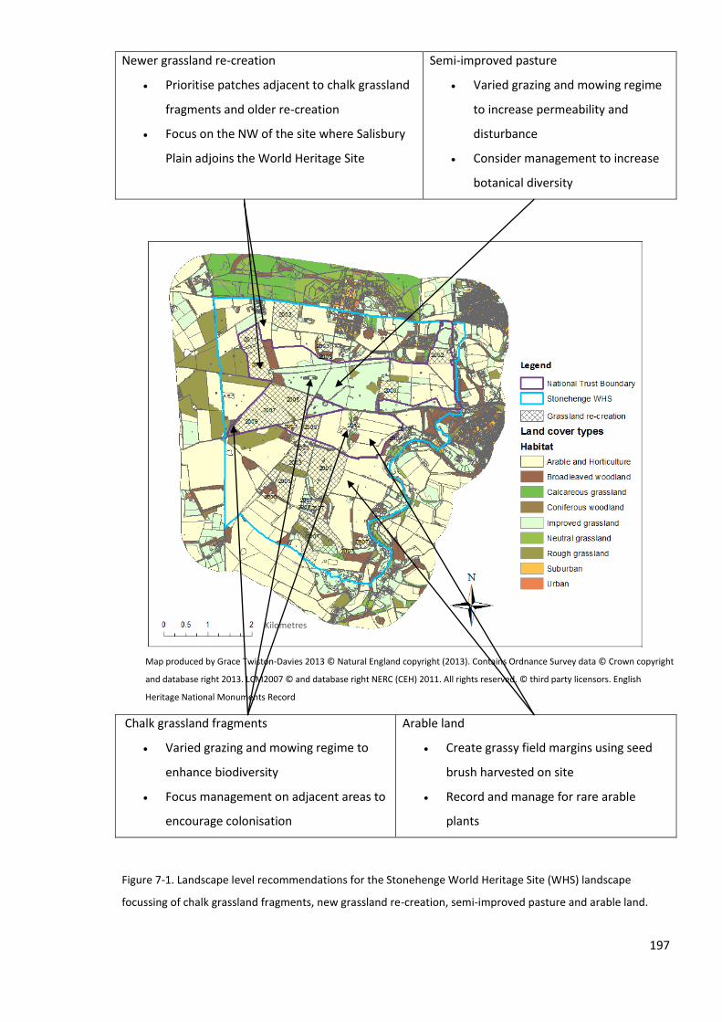
197
Newer grassland re-creation
Prioritise patches adjacent to chalk grassland
fragments and older re-creation
Focus on the NW of the site where Salisbury
Plain adjoins the World Heritage Site
Semi-improved pasture
Varied grazing and mowing regime
to increase permeability and
disturbance
Consider management to increase
botanical diversity
Chalk grassland fragments
Varied grazing and mowing regime to
enhance biodiversity
Focus management on adjacent areas to
encourage colonisation
Arable land
Create grassy field margins using seed
brush harvested on site
Record and manage for rare arable
plants
Figure 7-1. Landscape level recommendations for the Stonehenge World Heritage Site (WHS) landscape
focussing of chalk grassland fragments, new grassland re-creation, semi-improved pasture and arable land.
Kilometres
Map produced by Grace Twiston-Davies 2013 © Natural England copyright (2013). Contains Ordnance Survey data © Crown copyright
and database right 2013. LCM2007 © and database right NERC (CEH) 2011. All rights reserved. © third party licensors. English
Heritage National Monuments Record
198
7.5 Future research recommendations
The aims of this study covered some of the current knowledge gaps in landscape scale restoration
and the results have highlighted the next set of research questions detailed below.
There are a variety of factors that have an impact of the effect of restoration actions on biodiversity
enhancement and landscape connectivity. The scale and therefore, objectives of the policy that
restoration actions are conducted at can be vital as there is often a mismatch between the scale of
ecological processes and the scale of policy and management especially as governance and
administrative boundaries are often smaller than large scale ecological processes such as
metapopulation dynamics and ecosystem services (Guerrero et al. 2013; Henle et al. 2010; Young et
al. 2005). International policies may cover these large scale ecological processes (e.g. Natura 2000
network) but the National (e.g. Sites of Special Scientific Interest) and Local (e.g. Local Nature
Reserves) policies may not be effective in increasing biodiversity and landscape connectivity (Lawton
et al. 2010). There are also the constraints and objectives of the coordination method e.g. Agri-
environment schemes and New Environmental Land Management Scheme and these may not
benefit all plants and animals (Andersson et al. 2013; Pocock et al. 2012). Additionally landscape
scale restoration requires the collaboration and cooperation of many land owners and stake-holders
(Menz et al. 2013; Young et al. 2005), these will not all have same objectives or training. Also what
type of habitat is restored and for what target species can be an crucial factor in whether restoration
has a positive effect on the biodiversity and connectivity of the target habitat and organism
(Andersson et al. 2013; Fuentes-Montemayor et al. 2011; Pocock et al. 2012).
7.5.1 Are results transferable to all landscape scale grassland restoration in European temperate
grasslands?
This study provides an example of a landscape scale grassland restoration project, other examples
are available (Conrad & Tischew 2011; Fagan et al. 2008; Kiehl et al. 2006; Lengyel et al. 2012;
Piqueray et al. 2011; Prach & Walker 2011), but few combine evaluative methods at a range of
spatial scales and investigate the colonisation of these new habitats by mobile organisms. It is
therefore apparent that future research that investigates the ecological implications of a collection
of landscape scale restoration projects together, that evaluates the landscape scale implications of
habitat restoration and that uses colonisation data to measure success would be beneficial.
Additional research that focuses on the combined evaluation of landscape scale restoration projects
would provide an overview of the application and ecological benefits of restoration techniques at a
landscape scale and the subsequent management recommendations. These types of project have to
include early input from relevant stakeholders (Land managers, conservation NGOs and policy etc)
and clear links to uptake of findings if they are to have real world impact. A meta-analysis of

199
grassland restoration projects and the implications of the results for management is suggested or
alternatively, a collaborative research project involving sites of grassland recreation across Europe.
This would overcome the limitations of the transferability of conclusions based on the results from a
single study area which is recommended for future restoration evaluation (Ruiz-Jaen & Aide 2005).
Future research that investigates the landscape connectivity of existing sites of grassland restoration
is also advocated to quantify the impact of landscape scale grassland restoration on the functional
connectivity of the wider landscape. This would involve the spatial analysis of maps covering a range
of landscape scale restoration projects and evaluating them using some of the methods in this study
including cost-distance analysis, habitat landscape metrics and target taxa with different mobility
and ecological characteristics.
Current landscape scale restoration projects would benefit from additional research on evaluating
the progression of sites by the colonisation of target mobile taxa and the subsequent ecological
interactions.
7.5.2 How important is the behaviour of mobile taxa for landscape restoration and connectivity?
The behaviour of mobile organisms at habitat boundaries is a component in measuring and
evaluating landscape connectivity (Tischendorf & Fahrig 2000) and metapopulation dynamics (Heinz
et al. 2006). Therefore more research that includes behavioural research of mobile taxa, more
experimental studies and the investigation of behaviour at a range of chalk grassland fragments at
more than one study area, area recommended.
Experimental studies that use microcosms to investigate the behaviour of Lepidoptera at habitat,
resource and structural boundaries are recommended, (see examples in Bergman et al. 2007;
Merckx et al. 2003). These would benefit from being located using a large study area to increase the
replication of experimental plots and to reduce the compounding effects of the surrounding
landscape (thus not having the limitation of the study in Chapter 5). Studies that combine a variety
of dispersal and behavioural methods are also advocated as behaviour may be best interpreted for
conservation actions when used in combination with other methods of mark and recapture and
genetic analysis for conservation strategies (Leidner & Haddad 2011). Investigating the behaviour of
individuals in the matrix land cover is also advocated as this provides another measure of landscape
connectivity (Tischendorf & Fahrig 2000).
Behavioural studies across different restoration projects would offer more replication and
comparison and enable transferable and universal management recommendation for grassland
restoration projects to be made. A selection of restoration sites across the UK or Europe where
behaviour at habitat boundaries and in the matrix could be investigated and compared is
recommended.
200
7.5.3 What sort of targeted restoration measures would be best for enhancing landscape
connectivity?
Research into what restoration strategies are best for different landscapes is required. There are
guidelines for different types of landscapes depending on the degree of fragmentation and
degradation (McIntyre & Hobbs 1999) but these have not been evaluated using a selection of real
landscapes.
This research would involve assessing the best set of restorative and management options for a
particular landscape by comparing strategies with different aims. For example, at the Stonehenge
World Heritage Site, landscape connectivity could measured and compared between best practice
recommendations of restorative actions (Lawton et al. 2010; McIntyre & Hobbs 1999) with
management that targets either sites of, (i) highest matrix permeability, (ii) least permeable or, (iii)
intermediate permeability or, (iv) specific habitat patches as described in section (7.4.3). It would
also be recommended to compare these to random selection of sites for restoration and to compare
landscape connectivity under these scenarios with and without Agri-environment scheme options
for grassy field margins in arable land. This has been done using scenarios for woodland (Watts et al.
2010) and similar methods could be used.
7.5.4 What should the aim of restoration be?
The effect of restoration measures of biodiversity enhancement and landscape connectivity is
commonly measured in the short term as the similarity of diversity, vegetation structure and
ecological processes to those of the reference site (Ruiz-Jaen & Aide 2005). However, the effect of
restoration in the long term is more complex to measure as requires the presence of functional
groups required for long-term stability, resilience to natural disturbances and self-sustainability (SER
2004). The restoration of ecological networks is vital for ecosystem services and the long term
stability of these systems although is not always a result from restored communities and is not
always measured (Forup et al. 2008; Henson et al. 2009).
To evaluate restoration projects in these ways requires a long-term commitment to monitoring and
highlights that a set of restoration aims for the shot, medium and long term is recommended with
measurable goals that combine similarity to reference habitat patches, ecological process and
interactions and the long term sustainability. To achieve this collaboration between scientists, land
managers and policy makers is required (Menz et al. 2013; Young 2000). Additionally, research into
future threats to semi-natural grasslands and how this will change management recommendations
such as climate change is required as these will need to be adaptively managed in the future
(Lindenmayer et al. 2008; Poschlod & WallisDeVries 2002).

201
7.6 Conclusion
This study explored and highlighted landscape connectivity as a key to effective habitat restoration
for butterflies in lowland agricultural landscapes. The behaviour of Lepidoptera at habitat and
resource boundaries, their species richness and community compositions in restoration habitat and
the structural and functional connectivity of the landscape is investigated. The results illustrated that
there can be relatively rapid enhancement of biodiversity and landscape connectivity for
Lepidoptera associated with grasslands, even new grassland re-creation can increase boundary
crossing behaviour and the functional connectivity of the landscape has increased for this group as a
result of the restoration project. However, species with low mobility and/or specialist larval host
plants that do not establish in the grassland re-creation fields are restricted to the chalk grassland
fragments and will require targeted management and conservation in the future to encourage
colonisation of new habitats.
This study highlights that a range of management options at the habitat boundary, habitat patch and
landscape scales are required to enhance landscape connectivity and thereby increase the rate at
which the restoration of habitats at a landscape scale can achieve improvements for the biodiversity
of target taxa. Restoration that improves biodiversity and landscape connectivity starts from the
selection of appropriate seed source and location of receptor habitat patches, to ongoing targeted
management right through to the consideration of the landscape context in which grassland
restoration occurs.
Landscape connectivity is important as a connected and diverse landscape is more resilient and
adaptable to land-use, ecological, community and climate change. In the UK one mechanism for
implementing this is through site specific and targeted Agri-environment schemes. Measures of the
effect of restoration on biodiversity and landscape connectivity will need to evolve; currently, for
conditions need to represent that of the target habitat. However, for conservation, heterogeneity
and adaptation to change are also important and this may call for a paradigm shift in the aims and
objectives of habitat restoration.
Landscape scale restoration will require cooperation, collaboration and a shared vision from policy
makers, land owners and managers. This collaborative approach is the only successful route given
the complexity of landscape scale restoration and the many stakeholders responsible for its future
success. Interdisciplinary and pan-European collaborative research into the restoration of habitats at
a landscape scale is therefore advocated.
202
Chapter 8
8.1 Appendix A
8.1.1 Twiston-Davies. G., J. Mitchley, and S. R. Mortimer. 2011. The Stonehenge Landscape
Restoration Project- Conservation opportunities for rare butterflies? Aspects of Applied Biology.
108. 259-265.
8.1.2 Twiston-Davies. G., S. R. Mortimer, and J. Mitchley. (In press). Restoration of species rich
grassland in the Stonehenge World Heritage Site, UK. In: Kiehl. K., (Ed). Guidelines for native seed
production and grassland restoration. Cambridge Scholars.
8.2 Appendix B, C, D and E on Disc
Chapter 9 References
Allen, R., and P. Brash. 2008. Nature Conservation Evaluation 2007 Survey. The National Trust.
Conservation Directorate, Stonehenge Wiltshire.
Andersson, G. K. S., K. Birkhofer, M. Rundlöf, and H. G. Smith. 2013. Landscape heterogeneity and
farming practice alter the species composition and taxonomic breadth of pollinator
communities. Basic and Applied Ecology 14:540-546.
Anon. 1998. Lowland Calcareous grassland. UK Biodiversity group: Tranche 2 Action Plans.
Antwi, E. K., R. Krawczynski, and G. Wiegleb. 2008. Detecting the effect of disturbance on habitat
diversity and land cover change in a post-mining area using GIS. Landscape and Urban
Planning 87:22-32.
Asher, J., M. S. Warren, R. Fox, P. T. Harding, G. Jeffcoate, and S. Jeffcoate 2001. The Millennium
Atlas of Butterflies of Britain and Ireland. Oxford University Press, Oxford.
Auffret, A. G., R. Schmucki, J. Reimark, and S. A. O. Cousins. 2012. Grazing networks provide useful
functional connectivity for plants in fragmented systems. Journal of Vegetation Science
23:970-977.

203
Aviron, S., F. Burel, J. Baudry, and N. Schermann. 2005. Carabid assemblages in agricultural
landscapes: impacts of habitat features, landscape context at different spatial scales and
farming intensity. Agriculture, Ecosystems & Environment 108:205-217.
Aviron, S., P. Kindlmann, and F. Burel. 2007. Conservation of butterfly populations in dynamic
landscapes: The role of farming practices and landscape mosaic. Ecological Modelling
205:135-145.
Baguette, M. 2003. Long distance dispersal and landscape occupancy in a metapopulation of the
cranberry fritillary butterfly. Ecography 26:153-160.
Baguette, M., S. Blanchet, D. Legrand, V. M. Stevens, and C. Turlure. 2013. Individual dispersal,
landscape connectivity and ecological networks. Biological Reviews 88:310-326.
Baguette, M., J. Clobert, and N. Schtickzelle. 2011. Metapopulation dynamics of the bog fritillary
butterfly: experimental changes in habitat quality induced negative density-dependent
dispersal. Ecography 34:170-176.
Barbosa, O., and P. A. Marquet. 2002. Effects of forest fragmentation on the beetle assemblage at
the relict forest of Fray Jorge, Chile. Oecologia 132:296-306.
Bartomeus, I., S. G. Potts, I. Steffan-Dewenter, B. E. Vaissiere, M. Woyciechowski, K. M. Krewenka, T.
Tscheulin, S. P. M. Roberts, H. Szentgyorgyi, C. Westphal, and R. Bommarco. 2014.
Contribution of insect pollinators to crop yield and quality varies with agricultural
intensification. PeerJ 2:e328.
Bartuszevige, A. M., D. L. Gorchov, and L. Raab. 2006. The relative importance of landscape and
community features in the invasion of an exotic shrub in a fragmented landscape. Ecography
29:213-222.
Batary, P., B. Andras, D. Kleijn, and T. Tscharntke. 2011. Landscape-moderated biodiversity effects of
agri-environmental management: a meta-analysis. Proceedings of the Royal Society B-
Biological Sciences 278:1894-1902.
Batary, P., A. Holzschuh, K. M. Orci, F. Samu, and T. Tscharntke. 2012. Responses of plant, insect and
spider biodiversity to local and landscape scale management intensity in cereal crops and
grasslands. Agriculture Ecosystems & Environment 146:130-136.
Benini, L., V. Bandini, D. Marazza, and A. Contin. 2010. Assessment of land use changes through an
indicator-based approach: A case study from the Lamone river basin in Northern Italy.
Ecological Indicators 10:4-14.
Bennie, J., M. O. Hill, R. Baxter, and B. Huntley. 2006. Influence of slope and aspect on long-term
vegetation change in British chalk grasslands. Journal of Ecology 94:355-368.
Benton, T. G., J. A. Vickery, and J. D. Wilson. 2003. Farmland biodiversity: is habitat heterogeneity
the key? Trends in Ecology & Evolution 18:182-188.
204
Berg, A., K. Ahrne, E. Ockinger, R. Svensson, and B. Soderstrom. 2011. Butterfly distribution and
abundance is affected by variation in the Swedish forest-farmland landscape. Biological
Conservation 144:2819-2831.
Berg, A., K. Ahrne, E. Ockinger, R. Svensson, and J. Wissman. 2013. Butterflies in semi-natural
pastures and power-line corridors - effects of flower richness, management, and structural
vegetation characteristics. Insect Conservation and Diversity 6:639-657.
Berggren, A., B. Birath, and O. Kindvall. 2002. Effect of corridors and habitat edges on dispersal
behavior, movement rates, and movement angles in Roesel's bush-cricket (Metrioptera
roeseli). Conservation Biology 16:1562-1569.
Berggren, A., A. Carlson, and O. Kindvall. 2001. The effect of landscape composition on colonization
success, growth rate and dispersal in introduced bush-crickets Metrioptera roeseli. Journal of
Animal Ecology 70:663-670.
Bergman, M., K. Gotthard, D. Berger, M. Olofsson, D. J. Kemp, and C. Wiklund. 2007. Mating success
of resident versus non-resident males in a territorial butterfly. Proceedings of the Royal
Society B-Biological Sciences 274:1659-1665.
Beyer, L. J., and C. B. Schultz. 2010. Oviposition selection by a rare grass skipper Polites mardon in
montane habitats: Advancing ecological understanding to develop conservation strategies.
Biological Conservation 143:862-872.
Biesmeijer, J. C., S. P. M. Roberts, M. Reemer, R. Ohlemueller, M. Edwards, T. Peeters, A. P.
Schaffers, S. G. Potts, R. Kleukers, C. D. Thomas, J. Settele, and W. E. Kunin. 2006. Parallel
declines in pollinators and insect-pollinated plants in Britain and the Netherlands. Science
313:351-354.
Bink, F. A. 1992. Ecologische atlas van de dagvlinders van Nordwest-Europa. Haarlem Schuyt.
Binzenhofer, B., B. Schroder, B. Strauss, R. Biedermann, and J. Settele. 2005. Habitat models and
habitat connectivity analysis for butterflies and burnet moths - The example of Zygaena
carniolica and Coenonympha arcania. Biological Conservation 126:247-259.
Bloom, S. A. 1981. Similarity indeces in community studies - potential pitfalls. Marine Ecology
Progress Series 5:125-128.
Brudvig, L. A. 2011. The restoration of Biodiversity: Where has reserach been and where does it
need to go? American Journal of Botany 98:549-558.
Brudvig, L. A., S. A. Wagner, and E. I. Damschen. 2012. Corridors promote fire via connectivity and
edge effects. Ecological Applications 22:937-946.
Brueckmann, S. V., J. Krauss, and I. Steffan-Dewenter. 2010. Butterfly and plant specialists suffer
from reduced connectivity in fragmented landscapes. Journal of Applied Ecology 47:799-809.

205
Bulman, C. R., R. J. Wilson, A. R. Holt, L. G. Bravo, R. I. Early, M. S. Warren, and C. D. Thomas. 2007.
Minimum viable metapopulation size, extinction debt, and the conservation of a declining
species. Ecological Applications 17:1460-1473.
Buri, P., R. Arlettaz, and J. Y. Humbert. 2013. Delaying mowing and leaving uncut refuges boosts
orthopterans in extensively managed meadows: Evidence drawn from field-scale
experimentation. Agriculture Ecosystems & Environment 181:22-30.
Calabrese, J. M., and W. F. Fagan. 2004. A comparison-shopper's guide to connectivity metrics.
Frontiers in Ecology and the Environment 2:529-536.
Calaclura, B., and O. Spinell. 2008. Management of Natura 2000 habitats. 6210 Semi-natural dry
grasslands and scrubland facies on calcareous substrates (Festuco-Brometalia). European
Commission.
Campbell, H. 2009. Monitoring the Success of Calcicolous Grassland Reversion at Stonehenge. School
of Biological Sciences. University of Reading, Reading, UK.
Carvalheiro, L. G., W. E. Kunin, and J. C. Biesmeijer. 2013. Species Richness declines and biotic
homogenization have slowed down for NW-European pollinators and plants. Ecology Letters
16:1416-1417.
Carvell, C. 2002. Habitat use and conservation of bumblebees (Bombus spp.) under different
grassland management regimes. Biological Conservation 103:33-49.
Catchpole, R. 2006. Planning for Biodiversity- opportunity mapping and habitat networks in practice:
a technical guide. English Nature Research Reports No. 687.
Chen, I. C., H. J. Shiu, S. Benedick, J. D. Holloway, V. K. Cheye, H. S. Barlow, J. K. Hill, and C. D.
Thomas. 2009. Elevation increases in moth assemblages over 42 years on a tropical
mountain. Proceedings of the National Academy of Sciences of the United States of America
106:1479-1483.
Chippindale, C. 1983. Stonehenge Complete. Thames and Hudson, Leipzig.
Clausen, H. D., H. B. Holbeck, and J. Reddersen. 2001. Factors influencing abundance of butterflies
and burnet moths in the uncultivated habitats of an organic farm in Denmark. Biological
Conservation 98:167-178.
Clobert, J., R. A. Ims, and F. Rousset 2004. Causes, Mechanisms and Consequences of Dispersal In:
Hanski. I and Gaggiotti. O. E. 2004. Ecology, Genetics and Evolution of Metapopulations.
Elsevier Inc, San Diego.
Collinge, S. K. 2000. Effects of grassland fragmentation on insect species loss, colonization, and
movement patterns. Ecology 81:2211-2226.
Conrad, M. K., and S. Tischew. 2011. Grassland restoration in practice: Do we achieve the targets? A
case study from Saxony-Anhalt/Germany. Ecological Engineering 37:1149-1157.

206
Conradt, L., E. J. Bodsworth, T. J. Roper, and C. D. Thomas. 2000. Non-random dispersal in the
butterfly Maniola jurtina: implication for metapopulation models. Proceedings of the Royal
Society B-Biological Sciences 267:1505-1570.
Conradt, L., and T. J. Roper. 2006. Nonrandom movement behavior at habitat boundaries in two
butterfly species: Implications for dispersal. Ecology 87:125-132.
Cowley, M. J. R., C. D. Thomas, D. B. Roy, R. J. Wilson, J. L. Leon-Cortes, D. Gutierrez, C. R. Bulman, R.
M. Quinn, D. Moss, and K. J. Gaston. 2001. Density-distribution relationships in British
butterflies. I. The effect of mobility and spatial scale. Journal of Animal Ecology 70:410-425.
Crawley, M. J. 2007. The R Book. John Wiley and Sons Ltd, Chichester.
Craythorne, R. 2007. Grassland Reversion at Stonehenge- Monitoring and Assessment. School of
Biological Sciences. University of Reading, Reading, UK.
Cristescu, R. H., J. Rhodes, C. Frere, and P. B. Banks. 2013. Is restoring flora the same as restoring
fauna? Lessons learned from koalas and mining rehabilitation. Journal of Applied Ecology
50:423-431.
Crofts, A., and R. G. Jefferson. 1999. The Lowland Grassland Management Handbook (2nd edition).
English Nature/The Wildlife Trusts.
Curran, P., D. Smedley, P. Thompson, and A. T. Knight. 2012. Mapping restoration opportunity for
collaborating with land managers in a carbon credit-funded restoration program in the
Makana municipality, Eastern Cape, South Africa. Restoration Ecology 20:56-64.
Darvill, T. 2007. Stonehenge the Biography of a Landscape. Tempus, Stroud.
Davies, H., T. M. Brereton, D. B. Roy, and R. Fox. 2007. Government targets for protected area
management: will threatened butterflies benefit? Biodiversity and Conservation 16:3719-
3736.
Davies, K. F., C. R. Margules, and K. F. Lawrence. 2000. Which traits of species predict population
declines in experimental forest fragments? Ecology 81:1450-1461.
Davis, J. D., D. M. Debinski, and B. J. Danielson. 2007. Local and landscape effects on the butterfly
community in fragmented Midwest USA prairie habitats. Landscape Ecology 22:1341-1354.
de Bello, F., J. N. Price, T. Münkemüller, J. Liira, M. Zobel, W. Thuiller, P. Gerhold, L. Götzenberger, S.
Lavergne, J. Lepš, K. Zobel, and M. Pärtel. 2012. Functional species pool framework to test
for biotic effects on community assembly. Ecology 93:2263-2273.
Debinski, D. M., and R. D. Holt. 2000. A survey and overview of habitat fragmentation experiments.
Conservation Biology 14:342-355.
DEFRA. 2009. England biodiversity strategy indicators- A1 (b) populations of butterflies on farmland
in England.

207
Delattre, T., F. Burel, A. Humeau, V. M. Stevens, P. Vernon, and M. Baguette. 2010a. Dispersal mood
revealed by shifts from routine to direct flights in the meadow brown butterfly Maniola
jurtina. Oikos 119:1900-1908.
Delattre, T., J.-B. Pichancourt, F. Burel, and P. Kindlmann. 2010b. Grassy field margins as potential
corridors for butterflies in agricultural landscapes: A simulation study. Ecological Modelling
221:370-377.
Delattre, T., P. Vernon, and F. Burel. 2013. An agri-environmental scheme enhances butterfly
dispersal in European agricultural landscapes. Agriculture Ecosystems & Environment
166:102-109.
Dennis, R. L. H., J. G. Hodgson, R. Grenyer, T. G. Shreeve, and D. B. Roy. 2004. Host plants and
butterfly biology. Do host-plant strategies drive butterfly status? Ecological Entomology
29:12-26.
Dennis, R. L. H., T. G. Shreeve, and H. Van Dyck. 2003. Towards a functional resource-based concept
for habitat: a butterfly biology viewpoint. Oikos 102:417-426.
Deri, E., T. Magura, R. Horvath, M. Kisfali, G. Ruff, S. Lengyel, and B. Tothmeresz. 2011. Measuring
the short-term success of grassland restoration: the use of habitat affinity indices in
ecological restoration. Restoration Ecology 19:520-528.
Diacon-Bolli, J., T. Dalang, R. Holderegger, and M. Bürgi. 2012. Heterogeneity fosters biodiversity:
Linking history and ecology of dry calcareous grasslands. Basic and Applied Ecology 13:641-
653.
Diamond, S. E., A. M. Frame, R. A. Martin, and L. B. Buckley. 2011. Species' traits predict phenological
responses to climate change in butterflies. Ecology 92:1005-1012.
Diekotter, T., R. Billeter, and T. O. Crist. 2008. Effects of landscape connectivity on the spatial
distribution of insect diversity in agricultural mosaic landscapes. Basic and Applied Ecology
9:298-307.
Diepenbrock, L. M., and D. L. Finke. 2013. Refuge for native lady beetles (Coccinellidae) in perennial
grassland habitats. Insect Conservation and Diversity 6:671-679.
Doerr, V. A. J., T. Barrett, and E. D. Doerr. 2011. Connectivity, dispersal behaviour and conservation
under climate change: a response to Hodgson et al. Journal of Applied Ecology 48:143-147.
Donald, P. F., and A. D. Evans. 2006. Habitat connectivity and matrix restoration: the wider
implications of agri-environment schemes. Journal of Applied Ecology 43:209-218.
Dover, J., and J. Settele. 2009. The influences of landscape structure on butterfly distribution and
movement: a review. Journal of Insect Conservation 13:3-27.
Dover, J. W., and G. L. A. Fry. 2001. Experimental simulation of some visual and physical components
of a hedge and the effects on butterfly behaviour in an agricultural landscape. Entomologia
Experimentalis Et Applicata 100:221-233.

208
Dover, J. W., A. Rescia, S. Fungarino, J. Fairburn, P. Carey, P. Lunt, R. L. H. Dennis, and C. J. Dover.
2010. Can hay harvesting detrimentally affect adult butterfly abundance? Journal of Insect
Conservation 14:413-418.
Driscoll, D. A., and T. Weir. 2005. Beetle responses to habitat fragmentation depend on ecological
traits, habitat condition, and remnant size. Conservation Biology 19:182-194.
Duelli, P., and M. K. Obrist. 2003. Regional biodiversity in an agricultural landscape: the contribution
of seminatural habitat islands. Basic and Applied Ecology 4:129-138.
Ebeling, A., A. M. Klein, J. Schumacher, W. W. Weisser, and T. Tscharntke. 2008. How does plant
richness affect pollinator richness and temporal stability of flower visits? Oikos 117:1808-
1815.
ECNC. 2010. European Centre for Nature Conservation. http://www.ecnc.org. Date accessed
09/09/2010.
Edwards, A. R., S. R. Mortimer, C. S. Lawson, D. B. Westbury, S. J. Harris, B. A. Woodcock, and V. K.
Brown. 2007. Hay strewing, brush harvesting of seed and soil disturbance as tools for the
enhancement of botanical diversity in grasslands. Biological Conservation 134:372-382.
European Commission. 2014. From Land Cover to Landscape Diversity in the European Union.
http://ec.europa.eu/agriculture/publi/landscape. Date accessed 20/08/2014.
European Commission. 2014. About Corine Land Cover.
http://ec.europa.eu/agriculture/publi/landscape/about.htm. Date acccessed 20/08/2014.
Ewers, R. M., S. Thorpe, and R. K. Didham. 2007. Synergistic interactions between edge and area
effects in a heavily fragmented landscape. Ecology 88:96-106.
Eycott, A. E., M. Marzano, and K. Watts. 2011. Filling evidence gaps with expert opinion: The use of
Delphi analysis in least-cost modelling of functional connectivity. Landscape and Urban
Planning 103:400-409.
Eycott, A. E., G. B. Stewart, L. M. Buyung-Ali, D. E. Bowler, K. Watts, and A. S. Pullin. 2012. A meta-
analysis on the impact of different matrix structures on species movement rates. Landscape
Ecology 27:1263-1278.
Fagan, K. C., R. F. Pywell, J. M. Bullock, and R. H. Marrs. 2008. Do restored calcareous grasslands on
former arable fields resemble ancient targets? The effect of time, methods and environment
on outcomes. Journal of Applied Ecology 45:1293-1303.
Fagan, K. C., R. F. Pywell, J. M. Bullock, and R. H. Marrs. 2010. The seed banks of English lowland
calcareous grasslands along a restoration chronosequence. Plant Ecology 208:199-211.
Fahrig, L. 2001. How much habitat is enough? Biological Conservation 100:65-74.
Fahrig, L. 2013. Rethinking patch size and isolation effects: the habitat amount hypothesis. Journal of
Biogeography 40:1649-1663.
Fibrophos. 2014. http://www.fibrophos.co.uk. Date accessed 01/03/2014.
209
Filz, K. J., J. O. Engler, J. Stoffels, M. Weitzel, and T. Schmitt. 2013. Missing the target? A critical view
on butterfly conservation efforts on calcareous grasslands in south-western Germany.
Biodiversity and Conservation 22:2223-2241.
Fleishman, E., C. Ray, P. Sjogren-Gulve, C. L. Boggs, and D. D. Murphy. 2002. Assessing the roles of
patch quality, area, and isolation in predicting metapopulation dynamics. Conservation
Biology 16:706-716.
Forup, M. L., K. S. E. Henson, P. G. Craze, and J. Memmott. 2008. The restoration of ecological
interactions: plant-pollinator networks on ancient and restored heathlands. Journal of
Applied Ecology 45:742-752.
Fox, R., M. S. Warren, J. Asher, T. Brereton, and D. Roy. 2007. The state of Britain's butterflies 2007,
Wareham, Dorset, UK.
Frampton, G. K., T. Cilgi, G. L. A. Fry, and S. D. Wratten. 1995. Effects of grassy banks on the dispersal
of some carabid beetles (Coleoptera, Carabidae) on farmland. Biological Conservation
71:347-355.
Fuentes-Montemayor, E., D. Goulson, and K. J. Park. 2011. The effectiveness of agri-environment
schemes for the conservation of farmland moths: assessing the importance of a landscape-
scale management approach. Journal of Applied Ecology 48:532-542.
Fuller, R. M. 1987. The changing extent and conservation interest of lowland grasslands in England
and Wales: A review of grassland surveys 1930–1984. Biological Conservation 40:281-300.
Gibbs, M., C. J. Breuker, and H. Van Dyck. 2010. Flight during oviposition reduces maternal egg
provisioning and influences offspring development in Pararge aegeria (L.). Physiological
Entomology 35:29-39.
Gibbs, M., and H. Van Dyck. 2009. Reproductive plasticity, oviposition site selection, and maternal
effects in fragmented landscapes. Behavioral Ecology and Sociobiology 64:1-11.
Gibbs, M., and H. Van Dyck. 2010. Butterfly flight activity affects reproductive performance and
longevity relative to landscape structure. Oecologia (Berlin) 163:341-350.
Gonzalez-Varo, J. P., J. C. Biesmeijer, R. Bommarco, S. G. Potts, O. Schweiger, H. G. Smith, I. Steffan-
Dewenter, H. Szentgyoergyi, M. Woyciechowski, and M. Vila. 2013. Combined effects of
global change pressures on animal-mediated pollination. Trends in Ecology & Evolution
28:524-530.
Goodwin, B. J., and L. Fahrig. 2002. How does landscape structure influence landscape connectivity?
Oikos 99:552-570.
Gossner, M. M., S. Getzin, M. Lange, E. Pašalić, M. Türke, K. Wiegand, and W. W. Weisser. 2013. The
importance of heterogeneity revisited from a multiscale and multitaxa approach. Biological
Conservation 166:212-220.

210
Guerrero, A. M., R. R. J. McAllister, J. Corcoran, and K. A. Wilson. 2013. Scale mismatches,
conservation planning, and the value of social-network analyses. Conservation Biology
27:35-44.
Guisan, A., R. Tingley, J. B. Baumgartner, I. Naujokaitis-Lewis, P. R. Sutcliffe, A. I. T. Tulloch, T. J.
Regan, L. Brotons, E. McDonald-Madden, C. Mantyka-Pringle, T. G. Martin, J. R. Rhodes, R.
Maggini, S. A. Setterfield, J. Elith, M. W. Schwartz, B. A. Wintle, O. Broennimann, M. Austin,
S. Ferrier, M. R. Kearney, H. P. Possingham, and Y. M. Buckley. 2013. Predicting species
distributions for conservation decisions. Ecology Letters 16:1424-1435.
Gurnell, J., S. P. Rushton, P. W. W. Lurz, A. W. Sainsbury, P. Nettleton, M. D. F. Shirley, C. Bruemmer,
and N. Geddes. 2006. Squirrel poxvirus: Landscape scale strategies for managing disease
threat. Biological Conservation 131:287-295.
Gustafson, E. J., and G. R. Parker. 1994. Using an index of habitat patch proximity for landscape
design. Landscape and Urban Planning 29:117-130.
Gutierrez, D. 2005. Effectiveness of existing reserves in the long-term protection of a regionally rare
butterfly. Conservation Biology 19:1586-1597.
Haaland, C., and L. F. Bersier. 2011. What can sown wildflower strips contribute to butterfly
conservation?: an example from a Swiss lowland agricultural landscape. Journal of Insect
Conservation 15:301-309.
Haddad, N. M. 1999. Corridor and distance effects on interpatch movements: A landscape
experiment with butterflies. Ecological Applications 9:612-622.
Haddad, N. M., and J. J. Tewksbury. 2005. Low-quality habitat corridors as movement conduits for
two butterfly species. Ecological Applications 15:250-257.
Hanski, I. 1998. Metapopulation dynamics. Nature 396:41-49.
Hanski, I., M. Kuussaari, and M. Nieminen. 1994. Metapopulation structure and migration in the
butterfly Melitaea-cinxia. Ecology 75:747-762.
Hanski, I., and O. Ovaskainen. 2000. The metapopulation capacity of a fragmented landscape. Nature
404:755-758.
Hardy, P. B., T. H. Sparks, N. J. B. Isaac, and R. L. H. Dennis. 2007. Specialism for larval and adult
consumer resources among British butterflies: implications for conservation. Biological
Conservation 138:440-452.
Haynes, K. J., and J. T. Cronin. 2003. Matrix composition affects the spatial ecology of a prairie
planthopper. Ecology 84:2856-2866.
Haynes, K. J., and J. T. Cronin. 2006. Interpatch movement and edge effects: the role of behavioral
responses to the landscape matrix. Oikos 113:43-54.
Haynes, K. J., T. Diekotter, and T. O. Crist. 2007a. Resource complementation and the response of an
insect herbivore to habitat area and fragmentation. Oecologia 153:511-520.
211
Haynes, K. J., F. P. Dillemuth, B. J. Anderson, A. S. Hakes, H. B. Jackson, S. E. Jackson, and J. T. Cronin.
2007b. Landscape context outweighs local habitat quality in its effects on herbivore dispersal
and distribution. Oecologia 151:431-441.
Heath, J. H., and A. M. Emmet 1985. The Moths and Butterlies of Great Britain and Ireland: Cossidae
to Heliodinidae. Harley Books.
Heer, P., J. Pellet, A. Sierro, and R. Arlettaz. 2013. Evidence-based assessment of butterfly habitat
restoration to enhance management practices. Biodiversity and Conservation 22:239-252.
Heinz, S. K., C. Wissel, and K. Frank. 2006. The viability of metapopulations: individual dispersal
behaviour matters. Landscape Ecology 21:77-89.
Helsen, K., M. Hermy, and O. Honnay. 2013. Spatial isolation slows down directional plant functional
group assembly in restored semi-natural grasslands. Journal of Applied Ecology 50:404-413.
Hendrickx, F., J. P. Maelfait, W. Van Wingerden, O. Schweiger, M. Speelmans, S. Aviron, I.
Augenstein, R. Billeter, D. Bailey, R. Bukacek, F. Burel, T. Diekotter, J. Dirksen, F. Herzog, J.
Liira, M. Roubalova, V. Vandomme, and R. Bugter. 2007. How landscape structure, land-use
intensity and habitat diversity affect components of total arthropod diversity in agricultural
landscapes. Journal of Applied Ecology 44:340-351.
Henle, K., K. F. Davies, M. Kleyer, C. Margules, and J. Settele. 2004. Predictors of species sensitivity to
fragmentation. Biodiversity and Conservation 13:207-251.
Henle, K., W. Kunin, O. Schweiger, D. S. Schmeller, V. Grobelnik, Y. Matsinos, J. Pantis, L. Penev, S. G.
Potts, I. Ring, J. Simila, J. Tzanopoulos, S. van den Hove, M. Baguette, J. Clobert, L. Excoffier,
E. Framstad, M. Grodzinska-Jurczak, S. Lengyel, P. Marty, A. Moilanen, E. Porcher, D. Storch,
I. Steffan-Dewenter, M. T. Sykes, M. Zobel, and J. Settele. 2010. Securing the conservation of
biodiversity across administrative levels and spatial, temporal, and ecological scales-
research needs and approaches of the SCALES project. Gaia-Ecological Perspectives for
Science and Society 19:187-193.
Henson, K. S. E., P. G. Craze, and J. Memmott. 2009. The restoration of parasites, parasitoids, and
pathogens to heathland communities. Ecology 90:1840-1851.
Hickling, R., D. B. Roy, J. K. Hill, R. Fox, and C. D. Thomas. 2006. The distributions of a wide range of
taxonomic groups are expanding polewards. Global Change Biology 12:450-455.
Hill, J. K., C. D. Thomas, R. Fox, M. G. Telfer, S. G. Willis, J. Asher, and B. Huntley. 2002. Responses of
butterflies to twentieth century climate warming: implications for future ranges.
Proceedings of the Royal Society of London Series B-Biological Sciences 269:2163-2171.
Hobbs, R. J. 2007. Setting effective and realistic restoration goals: Key directions for research.
Restoration Ecology 15:354-357.

212
Hodgson, J. A., A. Moilanen, B. A. Wintle, and C. D. Thomas. 2011. Habitat area, quality and
connectivity: striking the balance for efficient conservation. Journal of Applied Ecology
48:148-152.
Hodgson, J. A., C. D. Thomas, B. A. Wintle, and A. Moilanen. 2009. Climate change, connectivity and
conservation decision making: back to basics. Journal of Applied Ecology 46:964-969.
Hodgson, J. G., J. P. Grime, P. J. Wilson, K. Thompson, and S. R. Band. 2005. The impacts of
agricultural change (1963-2003) on the grassland flora of Central England: processes and
prospects. Basic and Applied Ecology 6:107-118.
Hughes, C. L., J. K. Hill, and C. Dytham. 2003. Evolutionary trade-offs between reproduction and
dispersal in populations at expanding range boundaries. Proceedings of the Royal Society of
London Series B-Biological Sciences 270:S147-S150.
Humbert, J.-Y., J. Ghazoul, N. Richner, and T. Walter. 2012. Uncut grass refuges mitigate the impact
of mechanical meadow harvesting on orthopterans. Biological Conservation 152:96-101.
Jacquemyn, H., C. Van Mechelen, R. Brys, and O. Honnay. 2011. Management effects on the
vegetation and soil seed bank of calcareous grasslands: An 11-year experiment. Biological
Conservation 144:416-422.
Jauker, F., T. Diekotter, F. Schwarzbach, and V. Wolters. 2009. Pollinator dispersal in an agricultural
matrix: opposing responses of wild bees and hoverflies to landscape structure and distance
from main habitat. Landscape Ecology 24:547-555.
JNCC 1990. Handbook for phase 1 habitat survey.
JNCC. 2010. Joint Nature Conservation Committee. http://www.jncc.gov.uk. Date accessed
11/06/2010.
Kahmen, S., P. Poschlod, and K. F. Schreiber. 2002. Conservation management of calcareous
grasslands. Changes in plant species composition and response of functional traits during 25
years. Biological Conservation 104:319-328.
Kalarus, K., P. Skorka, and P. Nowicki. 2013. Resource use in two contrasting habitat types raises
different challenges for the conservation of the dryad butterfly Minois dryas. Journal of
Insect Conservation 17:777-786.
Keller, D., M. J. van Strien, M. Herrmann, J. Bolliger, P. J. Edwards, J. Ghazoul, and R. Holderegger.
2013. Is functional connectivity in common grasshopper species affected by fragmentation
in an agricultural landscape? Agriculture Ecosystems & Environment 175:39-46.
Kiehl, K., A. Kirmer, T. W. Donath, L. Rasran, and N. Hölzel. 2010. Species introduction in restoration
projects –evaluation of different techniques for the establishment of semi-natural grasslands
in Central and Northwestern Europe. Basic and Applied Ecology 11:285-299.
Kiehl, K., and J. Pfadenhauer. 2007. Establishment and persistence of target species in newly created
Calcareous grasslands on former arable fields. Plant Ecology 189:31-48.

213
Kiehl, K., A. Thormann, and J. Pfadenhauer. 2006. Evaluation of initial restoration measures during
the restoration of calcareous grasslands on former arable fields. Restoration Ecology 14:148-
156.
King, C., G. Ballantyne, and P. G. Willmer. 2013. Why flower visitation is a poor proxy for pollination:
measuring single-visit pollen deposition, with implications for pollination networks and
conservation. Methods in Ecology and Evolution 4:811-818.
Kleijn, D., and F. van Langevelde. 2006. Interacting effects of landscape context and habitat quality
on flower visiting insects in agricultural landscapes. Basic and Applied Ecology 7:201-214.
Knight, A. T., R. M. Cowling, M. Difford, and B. M. Campbell. 2010. Mapping human and social
dimensions of conservation opportunity for the scheduling of conservation action on private
land. Conservation Biology. 24:1348-1358.
Kohler, F., J. Verhulst, R. van Klink, and D. Kleijn. 2008. At what spatial scale do high-quality habitats
enhance the diversity of forbs and pollinators in intensively farmed landscapes? Journal of
Applied Ecology 45:753-762.
Komonen, A., A. Grapputo, V. Kaitala, J. S. Kotiaho, and J. Paivinen. 2004. The role of niche breadth,
resource availability and range position on the life history of butterflies. Oikos 105:41-54.
Korpela, E. L., T. Hyvonen, S. Lindgren, and M. Kuussaari. 2013. Can pollination services, species
diversity and conservation be simultaneously promoted by sown wildflower strips on
farmland? Agriculture Ecosystems & Environment 179:18-24.
Kuefler, D., B. Hudgens, N. M. Haddad, W. F. Morris, and N. Thurgate. 2010. The conflicting role of
matrix habitats as conduits and barriers for dispersal. Ecology 91:944-950.
Kumar, S., S. E. Simonson, and T. J. Stohlgren. 2009. Effects of spatial heterogeneity on butterfly
species richness in Rocky Mountain National Park, CO, USA. Biodiversity and Conservation
18:739-763.
Langmaid, J. R., A. M. Emmet, and J. H. Heath 1989. The Butterflies of Great Britain and Ireland:
Hesperiidae-Nymphalidae. Harley Books.
Larsen, T. H., N. M. Williams, and C. Kremen. 2005. Extinction order and altered community structure
rapidly disrupt ecosystem functioning. Ecology Letters 8:538-547.
Lawson, C. R., J. Bennie, J. A. Hodgson, C. D. Thomas, and R. J. Wilson. 2014. Topographic
microclimates drive microhabitat associations at the range margin of a butterfly. Ecography
37:732-740.
Lawson, C. R., J. J. Bennie, C. D. Thomas, J. A. Hodgson, and R. J. Wilson. 2012. Local and landscape
management of an expanding range margin under climate change. Journal of Applied
Ecology 49:552-561.
Lawton, J. H., P. N. M. Brotherton, V. K. Brown, C. Elphick, A. Fitter, J. Forshaw, R. W. Haddow, S.
Hilborne, R. N. Leafe, G. M. Mace, M. P. Southgate, W. J. Sutherland, T. E. Tew, J. Varley, and

214
G. R. Wynne. 2010. Making Space for Nature: a review of England's wildlife sites and
ecological network. Report to Defra. UK.
Leidner, A. K., and N. Haddad. 2011. Combiningmeasures of dispersal to identify conservation
strategies in fragmented landscapes. Conservation Biology 25:1022-1031.
Lengyel, S., K. Varga, B. Kosztyi, L. Lontay, E. Deri, P. Torok, and B. Tothmeresz. 2012. Grassland
restoration to conserve landscape-level biodiversity: a synthesis of early results from a large-
scale project. Applied Vegetation Science 15:264-276.
Lenoir, L., and T. Lennartsson. 2010. Effects of timing of grazing on arthropod communities in semi-
natural grasslands. Journal of Insect Science 10.
Li, H., D. Li, T. Li, Q. Qiao, J. Yang, and H. Zhang. 2010. Application of least-cost path model to identify
a giant panda dispersal corridor network after the Wenchuan earthquake-case study of
Wolong Nature Reserve in China. Ecological Modelling 221:944-952.
Lindborg, R., J. Bengtsson, Å. Berg, S. A. O. Cousins, O. Eriksson, T. Gustafsson, K. P. Hasund, L.
Lenoir, A. Pihlgren, E. Sjödin, and M. Stenseke. 2008. A landscape perspective on
conservation of semi-natural grasslands. Agriculture, Ecosystems & Environment 125:213-
222.
Lindenmayer, D., R. J. Hobbs, R. Montague-Drake, J. Alexandra, A. Bennett, M. Burgman, P. Cale, A.
Calhoun, V. Cramer, P. Cullen, D. Driscoll, L. Fahrig, J. Fischer, J. Franklin, Y. Haila, M. Hunter,
P. Gibbons, S. Lake, G. Luck, C. MacGregor, S. McIntyre, R. M. Nally, A. Manning, J. Miller, H.
Mooney, R. Noss, H. Possingham, D. Saunders, F. Schmiegelow, M. Scott, D. Simberloff, T.
Sisk, G. Tabor, B. Walker, J. Wiens, J. Woinarski, and E. Zavaleta. 2008. A checklist for
ecological management of landscapes for conservation. Ecology Letters 11:78-91.
MacArthur, R. H., and E. O. Wilson 1967. The theory of island biogeography. Princeton University
Press.
Maccherini, S., and E. Santi. 2012. Long-term experimental restoration in a calcareous grassland:
identifying the most effective restoration strategies. Biological Conservation 146:123-135.
MAGIC. 2014. http://magic.gov.uk. Date accessed 14/01/2014.
Major, R. E., F. J. Christie, G. Gowing, G. Cassis, and C. A. M. Reid. 2003. The effect of habitat
configuration on arboreal insects in fragmented woodlands of south-eastern Australia.
Biological Conservation 113:35-48.
Marini, L., E. Öckinger, K.-O. Bergman, B. Jauker, J. Krauss, M. Kuussaari, J. Pöyry, H. G. Smith, I.
Steffan-Dewenter, and R. Bommarco. 2013. Contrasting effects of habitat area and
connectivity on evenness of pollinator communities. Ecography 37:544-551.
Matter, S. F., and J. Roland. 2002. An experimental examination of the effects of habitat quality on
the dispersal and local abundance of the butterfly Parnassius smintheus. Ecological
Entomology 27:308-316.

215
McGarigal, K., S. A. Cushman, and E. Ene. 2012. FRAGSTATS v4:Spatial Pattern Analysis Program for
Categorical and Continuous Maps. Computer software program produced by the authors at
the University of Massachsetts, Amherst. Available at the following web site:
http//www.umass.edu/landeco/research/fragstats/fragstats.html. Date accessed
09/01/2014.
McIntyre, S., and R. Hobbs. 1999. A framework for conceptualizing human effects on landscapes and
its relevance to management and research models. Conservation Biology 13:1282-1292.
Menendez, R., D. Gutierrez, and C. D. Thomas. 2002. Migration and Allee effects in the six-spot
burnet moth Zygaena filipendulae. Ecological Entomology 27:317-325.
Menz, M. H. M., K. W. Dixon, and R. J. Hobbs. 2013. Hurdles and Opportunities for Landscape-Scale
Restoration. Science 339:526-527.
Menz, M. H. M., R. D. Phillips, R. Winfree, C. Kremen, M. A. Aizen, S. D. Johnson, and K. W. Dixon.
2011. Reconnecting plants and pollinators: challenges in the restoration of pollination
mutualisms. Trends in Plant Science 16:4-12.
Merckx, T., R. E. Feber, R. L. Dulieu, M. C. Townsend, M. S. Parsons, N. A. D. Bourn, P. Riordan, and D.
W. MacDonald. 2009. Effect of field margins on moths depends on species mobility: field-
based evidence for landscape-scale conservation. Agriculture Ecosystems & Environment
129:302-309.
Merckx, T., and H. Van Dyck. 2007. Habitat fragmentation affects habitat-finding ability of the
speckled wood butterfly, Pararge aegeria L. Animal Behaviour 74:1029-1037.
Merckx, T., H. Van Dyck, B. Karlsson, and O. Leimar. 2003. The evolution of movements and
behaviour at boundaries in different landscapes: a common arena experiment with
butterflies. Proceedings of the Royal Society of London Series B-Biological Sciences
270:1815-1821.
Mitchell, M. G. E., E. M. Bennett, and A. Gonzalez. 2013. Linking landscape connectivity and
ecosystem service provision: current knowledge and research gaps. Ecosystems 16:894-908.
Mitchley, J., I. Jongepierova, and K. Fajmon. 2012. Regional seed mixtures for the re-creation of
species-rich meadows in the White Carpathian Mountains: results of a 10-yr experiment.
Applied Vegetation Science 15:253-263.
Mitchley, J., and P. Xofis. 2005. Landscape structure and management regime as indicators of
calcareous grassland habitat condition and species diversity. Journal for Nature Conservation
13:171-183.
Moilanen, A., and I. Hanski. 1998. Metapopulation dynamics: Effects of habitat quality and landscape
structure. Ecology 79:2503-2515.
Moilanen, A., and M. Nieminen. 2002. Simple connectivity measures in spatial ecology. Ecology
83:1131-1145.

216
Mortimer, S. R., R. G. Booth, S. J. Harris, and V. K. Brown. 2002. Effects of initial site management on
the Coleoptera assemblages colonising newly established chalk grassland on ex-arable land.
Biological Conservation 104:301-313.
Morton, D., C. Rowland, C. Wood, L. Meek, C. Marston, G. Smith, and I. C. Simpson. 2011. CS
Technical Report No 11/07 NERC/Centre for Ecology and Hydrology (CEH project number:
C03259).
Mouissie, A. M., P. Vos, H. M. C. Verhagen, and J. P. Bakker. 2005. Endozoochory by free-ranging,
large herbivores: Ecological correlates and perspectives for restoration. Basic and Applied
Ecology 6:547-558.
Natura England. 2008. Lowland calcareous grassland BAP priority habitat inventory for England.
version 2.0.1.
Natural England. 2012. Assessing whether created or restored grassland is BAP Priority Habitat in
Natural England Technical Information Note 110.
Natural England. 2014. Nature Improvement Areas (NIAs). Page Overview on Nature Improvement
Areas.
http://www.naturalengland.org.uk/ourwork/conservation/biodiversity/funding/nia/default.
aspx. Date accessed 06/01/2014.
Naumann, C. M., G. M. Tarmann, and W. G. Tremewan 1999. The Western Palaearctic Zygaenidae.
Apollo Books.
NCC (Nature Conservation Committee). 1986. The Management of Chalk Grasslands for Butterflies.
(JNCC) Focus on nature conservation.
Nieminen, M., H. Rita, and P. Uuvana. 1999. Body size and migration rate in moths. Ecography
22:697-707.
Ockinger, E., K.-O. Bergman, M. Franzen, T. Kadlec, J. Krauss, M. Kuussaari, J. Poyry, H. G. Smith, I.
Steffan-Dewenter, and R. Bommarco. 2012. The landscape matrix modifies the effect of
habitat fragmentation in grassland butterflies. Landscape Ecology 27:121-131.
Ockinger, E., M. Franzen, M. Rundlof, and H. G. Smith. 2009. Mobility-dependent effects on species
richness in fragmented landscapes. Basic and Applied Ecology 10:573-578.
Ockinger, E., and H. G. Smith. 2007a. Asymmetric dispersal and survival indicate population sources
for grassland butterflies in agricultural landscapes. Ecography 30:288-298.
Ockinger, E., and H. G. Smith. 2007b. Semi-natural grasslands as population sources for pollinating
insects in agricultural landscapes. Journal of Applied Ecology 44:50-59.
Ockinger, E., and H. Van Dyck. 2012. Landscape Structure Shapes Habitat Finding Ability in a
Butterfly. PLoS One 7.
Oliver, T., D. B. Roy, J. K. Hill, T. Brereton, and C. D. Thomas. 2010. Heterogeneous landscapes
promote population stability. Ecology Letters 13:473-484.

217
Ouin, A., S. Aviron, J. Dover, and F. Burel. 2004. Complementation/supplementation of resources for
butterflies in agricultural landscapes. Agriculture Ecosystems & Environment 103:473-479.
Ouin, A., M. Martin, and F. Burel. 2008. Agricultural landscape connectivity for the meadow brown
butterfly (Maniola jurtina). Agriculture Ecosystems & Environment 124:193-199.
Ovaskainen, O., A. D. Smith, J. L. Osborne, D. R. Reynolds, N. L. Carreck, A. P. Martin, K. Niitepold,
and I. Hanski. 2008. Tracking butterfly movements with harmonic radar reveals an effect of
population age on movement distance. Proceedings of the National Academy of Sciences of
the United States of America 105:19090-19095.
Pacha, M. J., and S. Petit. 2008. The effect of landscape structure and habitat quality on the
occurrence of Geranium sylvaticum in fragmented hay meadows. Agriculture, Ecosystems &
Environment 123:81-87.
Parmesan, C. 2007. Influences of species, latitudes and methodologies on estimates of phenological
response to global warming. Global Change Biology 13:1860-1872.
Pe'er, G., M. A. Tsianou, K. W. Franz, Y. G. Matsinos, A. D. Mazaris, D. Storch, L. Kopsova, J. Verboom,
M. Baguette, V. M. Stevens, and K. Henle. 2014. Toward better application of minimum area
requirements in conservation planning. Biological Conservation 170:92-102.
Pemberton, C. 2011. Monitoring the success of Chalk Grassland Restoration in the Stonehenge
Landscape. School of Biological Sciences. University of Reading, Reading, UK.
Pfadenhauer, J. 2001. Some remarks on the socio-cultural background of restoration ecology.
Restoration Ecology 9:220-229.
Pickens, B. A., and K. V. Root. 2009. Behavior as a tool for assessing a managed landscape: a case
study of the Karner blue butterfly. Landscape Ecology 24:243-251.
Piqueray, J., G. Bottin, L.-M. Delescaille, E. Bisteau, G. Colinet, and G. Mahy. 2011. Rapid restoration
of a species-rich ecosystem assessed from soil and vegetation indicators: The case of
calcareous grasslands restored from forest stands. Ecological Indicators 11:724-733.
Pither, J., and P. D. Taylor. 1998. An experimental assessment of landscape connectivity. Oikos
83:166-174.
Plue, J., and S. A. O. Cousins. 2013. Temporal dispersal in fragmented landscapes. Biological
Conservation 160:250-262.
Pocock, M. J. O., D. M. Evans, and J. Memmott. 2012. The robustness and restoration of a network of
ecological networks. Science 335:973-977.
Pollard, E., and T. J. Yates 1993. Monitoring Butterflies for Ecology and Conservation: The British
Butterfly Monitoring Scheme. Springer.
Poschlod, P., S. Kiefer, U. Trankle, S. Fischer, and S. Bonn. 1998. Plant species richness in calcareous
grasslands as affected by dispersability in space and time. Applied Vegetation Science 1:75-
90.

218
Poschlod, P., and M. F. WallisDeVries. 2002. The historical and socioeconomic perspective of
calcareous grasslands - lessons from the distant and recent past. Biological Conservation
104:361-376.
Potts, S. G., J. C. Biesmeijer, C. Kremen, P. Neumann, O. Schweiger, and W. E. Kunin. 2010. Global
pollinator declines: trends, impacts and drivers. Trends in Ecology & Evolution 25:345-353.
Powney, G. D., L. K. Broaders, and T. H. Oliver. 2012. Towards a measure of functional connectivity:
local synchrony matches small scale movements in a woodland edge butterfly. Landscape
Ecology 27:1109-1120.
Prach, K., I. Jongepierova, and K. Rehounkova. 2013. Large-scale restoration of dry grasslands on ex-
arable land using a regional seed mixture: establishment of target species. Restoration
Ecology 21:33-39.
Prach, K., and L. R. Walker. 2011. Four opportunities for studies of ecological succession. Trends in
Ecology & Evolution 26:119-123.
Prevedello, J. A., and M. V. Vieira. 2010. Does the type of matrix matter? A quantitative review of the
evidence. Biodiversity and Conservation 19:1205-1223.
Proença, V., and H. M. Pereira. 2013. Species–area models to assess biodiversity change in multi-
habitat landscapes: the importance of species habitat affinity. Basic and Applied Ecology
14:102-114.
Prugh, L. R., K. E. Hodges, A. R. E. Sinclair, and J. S. Brashares. 2008. Effect of habitat area and
isolation on fragmented animal populations. Proceedings of the National Academy of
Sciences of the United States of America 105:20770-20775.
Pywell, R. F., J. Bullock, D. Roy, P. Rothery, L. Warman, P. Bellamy, and K. Walker. 1999. A review of
the ecological characteristics of wildflower species in relation to the sucess of restoration.
Institute of Terrestrial Ecology, Centre for Ecology and Hydrology.
Pywell, R. F., J. M. Bullock, A. Hopkins, K. J. Walker, T. H. Sparks, M. J. W. Burke, and S. Peel. 2002.
Restoration of species-rich grassland on arable land: assessing the limiting processes using a
multi-site experiment. Journal of Applied Ecology 39:294-309.
Pywell, R. F., J. M. Bullock, D. B. Roy, L. I. Z. Warman, K. J. Walker, and P. Rothery. 2003. Plant traits
as predictors of performance in ecological restoration. Journal of Applied Ecology 40:65-77.
Pywell, R. F., M. S. Heard, R. B. Bradbury, S. Hinsley, M. Nowakowski, K. J. Walker, and J. M. Bullock.
2012. Wildlife-friendly farming benefits rare birds, bees and plants. Biology Letters 8:772-
775.
Racz, I. A., E. Deri, M. Kisfali, Z. Batiz, K. Varga, G. Szabo, and S. Lengyel. 2013. Early changes of
orthopteran assemblages after grassland restoration: a comparison of space-for-time
substitution versus repeated measures monitoring. Biodiversity and Conservation 22:2321-
2335.

219
Rakosy, L., and T. Schmitt. 2011. Are butterflies and moths suitable ecological indicator systems for
restoration measures of semi-natural calcareous grassland habitats? Ecological Indicators
11:1040-1045.
R Core Team. 2010. R: A language for statistical computing. R Foundation for statistical computing.
Version 2.12.0. URL http://www.R-project.org., Vienna, Austria.
R Core Team. 2013. R: A language for statistical computing. R Foundation for statistical computing.
Version 3.0.0. URL http://www.R-project.org, Vienna, Austria.
Reeve, J. D., J. T. Cronin, and K. J. Haynes. 2008. Diffusion models for animals in complex landscapes:
incorporating heterogeneity among substrates, individuals and edge behaviours. Journal of
Animal Ecology 77:898-904.
Renton, M., N. Shackelford, and R. J. Standish. 2012. Habitat restoration will help some functional
plant types persist under climate change in fragmented landscapes. Global Change Biology
18:2057-2070.
Ricketts, T. H. 2001. The matrix matters: effective isolation in fragmented landscapes. American
Naturalist 158:87-99.
Riedinger, V., M. Renner, M. Rundlof, I. Steffan-Dewenter, and A. Holzschuh. 2014. Early mass-
flowering crops mitigate pollinator dilution in late-flowering crops. Landscape Ecology
29:425-435.
Ries, L., and D. M. Debinski. 2001. Butterfly responses to habitat edges in the highly fragmented
prairies of Central Iowa. Journal of Animal Ecology 70:840-852.
Ries, L., and T. D. Sisk. 2008. Butterfly edge effects are predicted by a simple model in a complex
landscape. Oecologia 156:75-86.
Rodwell, J. 1992. British Plant Communities, Volume 3- Grasslands and Montane communities.
Cambridge University Press, Cambridge.
Roland, J., N. Keyghobadi, and S. Fownes. 2000. Alpine Parnassius butterfly dispersal: effects of
landscape and population size. Ecology 81:1642-1653.
Rook, A. J., B. Dumont, J. Isselstein, K. Osoro, M. F. WallisDeVries, G. Parente, and J. Mills. 2004.
Matching type of livestock to desired biodiversity outcomes in pastures - a review. Biological
Conservation 119:137-150.
Rosin, Z. M., L. Myczko, P. Skorka, M. Lenda, D. Moron, T. H. Sparks, and P. Tryjanowski. 2012.
Butterfly responses to environmental factors in fragmented calcareous grasslands. Journal of
Insect Conservation 16:321-329.
Ruiz-Jaen, M. C., and T. M. Aide. 2005. Restoration success: how is it being measured? Restoration
Ecology 13:569-577.
Rusterholz, H. P., and A. Erhardt. 2000. Can nectar properties explain sex-specific flower preferences
in the Adonis Blue butterfly Lysandra bellargus? Ecological Entomology 25:81-90.

220
Samnegard, U., A. S. Persson, and H. G. Smith. 2011. Gardens benefit bees and enhance pollination
in intensively managed farmland. Biological Conservation 144:2602-2606.
SCALES. 2014. Securing the Conservation of biodiversity across Administrative Levels and spatial,
temporal and Ecological Scales. http://www.scales-project.net/. Date accessed 21/02/2014.
Schneider, C., J. Dover, and G. L. A. Fry. 2003. Movement of two grassland butterflies in the same
habitat network: the role of adult resources and size of the study area. Ecological
Entomology 28:219-227.
Schtickzelle, N., and M. Baguette. 2003. Behavioural responses to habitat patch boundaries restrict
dispersal and generate emigration-patch area relationships in framented landscapes. Journal
of Animal Ecology 72:533-545.
Schultz, C. B., A. M. A. Franco, and E. E. Crone. 2012. Response of butterflies to structural and
resource boundaries. Journal of Animal Ecology 81:724-734.
Schumaker, N. H. 1996. Using landscape indices to predict habitat connectivity. Ecology 77:1210-
1225.
Schweiger, O., J. Settele, O. Kudrna, S. Klotz, and I. Kuhn. 2008. Climate change can cause spatial
mismatch of trophically interacting species. Ecology 89:3472-3479.
SER. 2004. Society for Ecological Restoration international science and policy working group. The SER
international primer on ecological restoration. Society for Ecological Restoration.
Severns, P. M., E. J. B. McIntire, and C. B. Schultz. 2013. Evaluating functional connectivity with
matrix behavior uncertainty for an endangered butterfly. Landscape Ecology 28:559-569.
Shreeve, T. G., and R. L. H. Dennis. 2011. Landscape scale conservation: resources, behaviour, the
matrix and opportunities. Journal of Insect Conservation 15:179-188.
Shreeve, T. G., R. L. H. Dennis, D. B. Roy, and D. Moss. 2001. An ecological classification of British
butterflies: Ecological attributes and biotope occupancy. Journal of Insect Conservation
5:145-161.
Skorka, P., P. Nowicki, M. Lenda, M. Witek, E. B. Sliwinska, J. Settele, and M. Woyciechowski. 2013.
Different flight behaviour of the endangered scarce large blue butterfly Phengaris teleius
(Lepidoptera: Lycaenidae) within and outside its habitat patches. Landscape Ecology 28:533-
546.
Slamova, I., J. Klecka, and M. Konvicka. 2013. Woodland and grassland mosaic from a butterfly
perspective: habitat use by Erebia aethiops (Lepidoptera: Satyridae). Insect Conservation
and Diversity 6:243-254.
Smart, S. 2001. MAVIS Plot Analyser. DART Computing.
Smith, M., J. Chetcuti, D. Moseley, and C. Quine. 2012. Addressing issues of conservation concern
based on principles of landscape ecology- application to quick wins and the long march.
Forest Research.

221
Stace, C. 2010. New Flora of the British Isles. Cambridge University Press, Cambridge.
Stamps, J. A., M. Buechner, and V. V. Krishnan. 1987. The Effects of Edge Permeability and Habitat
Geometry on Emigration from Patches of Habitat. American Naturalist 129:533-552.
Steffan-Dewenter, I., U. Munzenberg, C. Burger, C. Thies, and T. Tscharntke. 2002. Scale-dependent
effects of landscape context on three pollinator guilds. Ecology 83:1421-1432.
Steffan-Dewenter, I., and T. Tscharntke. 2002. Insect communities and biotic interactions on
fragmented calcareous grasslands - a mini review. Biological Conservation 104:275-284.
Stewart, K. E. J., N. A. D. Bourn, and J. A. Thomas. 2001. An evaluation of three quick methods
commonly used to assess sward height in ecology. Journal of Applied Ecology 38:1148-1154.
Sutherland, W. J., A. S. Pullin, P. M. Dolman, and T. M. Knight. 2004. The need for evidence-based
conservation. Trends in Ecology & Evolution 19:305-308.
Tambosi, L. R., A. C. Martensen, M. C. Ribeiro, and J. P. Metzger. 2014. A framework to optimize
biodiversity restoration efforts based on habitat amount and landscape connectivity.
Restoration Ecology 22:169-177.
Taylor, P. D., L. Fahrig, K. Henein, and G. Merriam. 1993. Connectivity is a vital element of landscape
structure. Oikos 68:571-572.
ter Braak, C. J. F., and P. Smilauer 2012. Canoco reference manual and user's guide: software for
ordination (version 5.0). Microcomputer Power, Ithaca, NY, USA.
Thomas, C. D. 2000. Dispersal and extinction in fragmented landscapes. Proceedings of the Royal
Society B-Biological Sciences 267:139-145.
Thomas, C. D., E. J. Bodsworth, R. J. Wilson, A. D. Simmons, Z. G. Davies, M. Musche, and L. Conradt.
2001a. Ecological and evolutionary processes at expanding range margins. Nature 411:577-
581.
Thomas, C. D., P. K. Gillingham, R. B. Bradbury, D. B. Roy, B. J. Anderson, J. M. Baxter, N. A. D. Bourn,
H. Q. P. Crick, R. A. Findon, R. Fox, J. A. Hodgson, A. R. Holt, M. D. Morecroft, N. J. O'Hanlon,
T. H. Oliver, J. W. Pearce-Higgins, D. A. Procter, J. A. Thomas, K. J. Walker, C. A. Walmsley, R.
J. Wilson, and J. K. Hill. 2012. Protected areas facilitate species' range expansions.
Proceedings of the National Academy of Sciences of the United States of America
109:14063-14068.
Thomas, J. A. 1983. The ecology and conservation of Lysandra bellargus (Lepidoptera, Lycaenidae) in
Britain. Journal of Applied Ecology 20:59-83.
Thomas, J. A. 2005. Monitoring change in the abundance and distribution of insects using butterflies
and other indicator groups. Philosophical Transactions of the Royal Society B-Biological
Sciences 360:339-357.
Thomas, J. A., N. A. D. Bourn, R. T. Clarke, K. E. Stewart, D. J. Simcox, G. S. Pearman, R. Curtis, and B.
Goodger. 2001b. The quality and isolation of habitat patches both determine where

222
butterflies persist in fragmented landscapes. Proceedings of the Royal Society of London
Series B-Biological Sciences 268:1791-1796.
Thomas, J. A., and R. T. Clarke. 2004. Extinction rates and butterflies - Response. Science 305:1563-+.
Thomas, J. A., D. J. Simcox, and R. T. Clarke. 2009. Successful conservation of a threatened Maculinea
butterfly. Science 325:80-83.
Thomas, J. A., M. G. Telfer, D. B. Roy, C. D. Preston, J. J. D. Greenwood, J. Asher, R. Fox, R. T. Clarke,
and J. H. Lawton. 2004. Comparative losses of British butterflies, birds, and plants and the
global extinction crisis. Science 303:1879-1881.
Thomson, J. R., A. J. Moilanen, P. A. Vesk, A. F. Bennett, and R. M. Nally. 2009. Where and when to
revegetate: a quantitative method for scheduling landscape reconstruction. Ecological
Applications 19:817-828.
Tischendorf, L., and L. Fahrig. 2000. On the usage and measurement of landcape connectivity. Oikos
90:7-19.
Toeroek, P., E. Vida, B. Deak, S. Lengyel, and B. Tothmeresz. 2011. Grassland restoration on former
croplands in Europe: an assessment of applicability of techniques and costs. Biodiversity and
Conservation 20:2311-2332.
Travis, J. M. J., M. Delgado, G. Bocedi, M. Baguette, K. Barton, D. Bonte, I. Boulangeat, J. A. Hodgson,
A. Kubisch, V. Penteriani, M. Saastamoinen, V. M. Stevens, and J. M. Bullock. 2013. Dispersal
and species' responses to climate change. Oikos 122:1532-1540.
Tropek, R., M. Hejda, T. Kadlec, and L. Spitzer. 2013. Local and landscape factors affecting
communities of plants and diurnal Lepidoptera in black coal spoil heaps: implications for
restoration management. Ecological Engineering 57:252-260.
Tscharntke, T., and R. Brandl. 2004. Plant-insect interactions in fragmented landscapes. Annual
Review of Entomology 49:405-430.
Tscharntke, T., I. Steffan-Dewenter, A. Kruess, and C. Thies. 2002. Characteristics of insect
populations on habitat fragments: a mini review. Ecological Research 17:229-239.
Twiston-Davies, G., S. R. Mortimer, and J. Mitchley in press. Restoration of species rich grassland in
the Stonehenge World Heritage Site, UK. In Kiehl. K., (Ed). Guidelines for native seed
production and grassland restoration Cambridge Scholars, Cambridge.
Uuemaa, E., U. Mander, and R. Marja. 2013. Trends in the use of landscape spatial metrics as
landscape indicators: a review. Ecological Indicators 28:100-106.
Valladares, G., A. Salvo, and L. Cagnolo. 2006. Habitat fragmentation effects on trophic processes of
insect-plant food webs. Conservation Biology 20:212-217.
van Noordwijk, C. G. E., P. Boer, A. A. Mabelis, W. Verberk, and H. Siepel. 2012a. Life-history
strategies as a tool to identify conservation constraints: a case-study on ants in chalk
grasslands. Ecological Indicators 13:303-313.

223
van Noordwijk, C. G. E., D. E. Flierman, E. Remke, M. F. WallisDeVries, and M. P. Berg. 2012b. Impact
of grazing management on hibernating caterpillars of the butterfly Melitaea cinxia in
calcareous grasslands. Journal of Insect Conservation 16:909-920.
van Swaay, C. A. M. 2002. The importance of calcareous grasslands for butterflies in Europe.
Biological Conservation 104:315-318.
Van Swaay, C. A. M., A. Cuttelod, S. Collins, D. Maes, M. Lopez Munguira, M. Sasic, J. Settele, R.
Verovnik, T. Verstrael, M. S. Warren, M. Wiemers, and I. Wynhof. 2010. European Red List of
Butterflies, Luxembourg.
Van Teeffelen, A. J. A., C. C. Vos, and P. Opdam. 2012. Species in a dynamic world: consequences of
habitat network dynamics on conservation planning. Biological Conservation 153:239-253.
Vergnes, A., I. Le Viol, and P. Clergeau. 2012. Green corridors in urban landscapes affect the
arthropod communities of domestic gardens. Biological Conservation 145:171-178.
Wagner, H. H., Y. Rico, H. Lehnert, and H. J. Boehmer. 2013. Process-based long-term evaluation of
an ecological network of calcareous grasslands connected by sheep herding. Ecography
36:374-382.
Walker, K. J., P. A. Stevens, D. P. Stevens, J. O. Mountford, S. J. Manchester, and R. F. Pywell. 2004.
The restoration and re-creation of species-rich lowland grassland on land formerly managed
for intensive agriculture in the UK. Biological Conservation 119:1-18.
WallisDeVries, M. F., and S. H. Ens. 2010. Effects of habitat quality and isolation on the colonization
of restored heathlands by butterflies. Restoration Ecology 18:390-398.
WallisDeVries, M. F., P. Poschlod, and J. H. Willems. 2002. Challenges for the conservation of
calcareous grasslands in northwestern Europe: integrating the requirements of flora and
fauna. Biological Conservation 104:265-273.
Warren, M. S., J. K. Hill, J. A. Thomas, J. Asher, R. Fox, B. Huntley, D. B. Roy, M. G. Telfer, S. Jeffcoate,
P. Harding, G. Jeffcoate, S. G. Willis, J. N. Greatorex-Davies, D. Moss, and C. D. Thomas. 2001.
Rapid responses of British butterflies to opposing forces of climate and habitat change.
Nature 414:65-69.
Watts, K., A. E. Eycott, P. Handley, D. Ray, J. W. Humphrey, and C. P. Quine. 2010. Targeting and
evaluating biodiversity conservation action within fragmented landscapes: an approach
based on generic focal species and least-cost networks. Landscape Ecology 25:1305-1318.
Watts, K., and P. Handley. 2010. Developing a functional connectivity indicator to detect change in
fragmented landscapes. Ecological Indicators 10:552-557.
Wiens, J. A. 1997. Metapopulation Dynamics and Landscape Ecology. Pages 43-62 in H. Ilkka, and E.
G. Michael, editors. Metapopulation Biology. Academic Press, San Diego.
Wilkerson, M. L. 2013. Invasive plants in conservation linkages: a conceptual model that addresses
an underappreciated conservation issue. Ecography 36:1319-1330.

224
Wilson, R. J., Z. G. Davies, and C. D. Thomas. 2010. Linking habitat use to range expansion rates in
fragmented landscapes: a metapopulation approach. Ecography 33:73-82.
Wilson, R. J., D. Gutierrez, J. Gutierrez, and V. J. Monserrat. 2007. An elevational shift in butterfly
species richness and composition accompanying recent climate change. Global Change
Biology 13:1873-1887.
Woodcock, B. A., J. M. Bullock, S. R. Mortimer, T. Brereton, J. W. Redhead, J. A. Thomas, and R. F.
Pywell. 2012a. Identifying time lags in the restoration of grassland butterfly communities: A
multi-site assessment. Biological Conservation 155:50-58.
Woodcock, B. A., J. M. Bullock, S. R. Mortimer, and R. F. Pywell. 2012b. Limiting factors in the
restoration of UK grassland beetle assemblages. Biological Conservation 146:136-143.
Woodcock, B. A., A. R. Edwards, C. S. Lawson, D. B. Westbury, A. J. Brook, S. J. Harris, V. K. Brown,
and S. R. Mortimer. 2008. Contrasting success in the restoration of plant and phytophagous
beetle assemblages of species-rich mesotrophic grasslands. Oecologia 154:773-783.
Woodcock, B. A., A. R. Edwards, C. S. Lawson, D. B. Westbury, A. J. Brook, S. J. Harris, G. Masters, R.
Booth, V. K. Brown, and S. R. Mortimer. 2010. The restoration of phytophagous beetles in
species-rich chalk grasslands. Restoration Ecology 18:638-644.
Woodcock, B. A., M. Edwards, J. Redhead, W. R. Meek, P. Nuttall, S. Falk, M. Nowakowski, and R. F.
Pywell. 2013. Crop flower visitation by honeybees, bumblebees and solitary bees:
behavioural differences and diversity responses to landscape. Agriculture Ecosystems &
Environment 171:1-8.
Young, C., A. Chadburn, and I. Bedu. 2009. Stonehenge World Heritage Site Management Plan 2009.
English Heritage, London, UK.
Young, T. P. 2000. Restoration ecology and conservation biology. Biological Conservation 92:73-83.
Young, T. P., D. A. Petersen, and J. J. Clary. 2005. The ecology of restoration: historical links,
emerging issues and unexplored realms. Ecology Letters 8:662-673.