Land Surface Processes - The Department of Geological Sciences

ang

Land Surface Modeling:

Past, Present and Future

Zong-Liang Yang

512-471-3824

[email protected]

http://www.geo.utexas.edu/climate

Department of Geological Sciences

Jackson School of Geosciences

1/3/2011

ang

Outline

• Introduction

• Land Surface Processes

• Land Surface Modeling

• Example 1: NCAR Community Land Model (CLM)

• Example 2: Noah LSM

• Summary

ang

Why Land

• Land research has direct societal relevance.

• Land provides us food, clothing, shelter, and infrastructure.

• Land is at the central stage for extreme weather and climate events.

• Land research is cross-disciplinary, and land processes cover all time and space scales.

ang

-Biogeochemistry

-Genetic bank

-Water

-Air

-Institutions

-Culture

-Technology

-Population

-Economic

LANDCOVER [Biophysically controlled]

Ecosystem goods & services

-clean air/water

-waste recycling

-food/fibre/fuel

-recreation

Ecological Problems

-pollution

-diseases

-food/fibre/fuel shortages

-overcrowding

DYNAMIC GLOBAL LAND TRANSITIONS

HUMAN DECISION MAKING

political/economic choices

Human

Systems

Ecological

Systems

LANDUSE [Human control]

Economic Problems

-poverty

-unequal wealth

-war

-globalization

Running 2006 4

ang

How do Human Activities Contribute to Climate Change and How do

They Compare with Natural Influences?

Foley et al. 2005

IPCC 2007

5

ang

BATS, SiB, …

6

PILPS

CLM

Land is an important component in weather and

climate models

Modified from IPCC 2007

Bucket

ang

What Are Land Surface Processes?

• Exchange processes with the atmosphere – Momentum

– Energy (reflected shortwave, emitted longwave, latent/sensible heat)

– Water (precipitation, evapotranspiration)

– Trace gases (CO2)/dusts/aerosols/pollutants

• Exchange processes with the ocean – Fresh water

– Sediments/nutrients

– Salinity

• Land-memory processes – Topography

– Snow/ice cover

– Soil moisture

– Vegetation

• Human activities – Land use (agriculture, afforestation, deforestation, urbanization,…)

– Land air/water pollution

ang

Do Land Surface Processes Matter to Climate Prediction?

Observed transient soil

moisture anomalies

can be more important

to accurately predict

mid-continental

summertime extreme

rainfalls (in USA) than

sea surface

temperatures

(Entekhabi et al.,

1999).

ang

Soil Moisture–Precipitation Feedback Loops

Pitman (2003)

ang

Land–Atmosphere Coupling Strength

The greatest land–

atmosphere coupling appears

to lie in arid-to-humid

transition zones, where soil

moisture anomalies strongly

influence precipitation

anomalies (Koster et al.,

Science, 2004).

The profile of soil moisture can be determined by the water table position (e.g., Levine and Salvucci, 1999).

Shallow groundwater table sustains surface vegetation, especially during drought (e.g., York et al., 2002).

Kim and Wang (2007) found

that soil moisture-induced

precipitation increase is

enhanced under wet summer

when vegetation phenology is

included in their model,

consistent with the findings of

others

(e.g., Dickinson and Henderson-Sellers, 1988; Hoffmann et al,. 2000; Matsui et al., 2005; Xue et al. 2006).

ang

What Are Land Surface Processes

• Land surface consists of

– urban areas, soil, vegetation, snow, topography, inland water (lake, river)

…

• Land surface processes describe

– exchanges of momentum, energy, water vapor, and other trace gases between

land surface and the overlying atmosphere

– states of land surface (e.g., soil moisture, soil temperature, canopy

temperature, snow water equivalent)

– characteristics of land surface (e.g., soil texture, surface roughness, albedo,

emissivity, vegetation type, cover extent, leaf area index, and seasonality)

ang

What Are Land Surface Processes

• Land surface processes function as

– lower boundary condition in Atmospheric Models

• Atmospheric Boundary Layer Simulation Climate Simulation

• Numerical Weather Prediction 4-D Data Assimilation

– upper boundary condition in Hydrological Models

• Water Resources Estimation; Crop Water Use; Runoff Simulation

– interface for coupled Atmospheric/Hydrological/Ecological Models

ang

Land Surface Models (LSMs)

• Computer code describing land surface processes (also called

LSSs, LSPs, SVATs)

– FORTRAN, C, C++, … ...

– Tens to thousands of lines

• There are a huge number of LSMs (100+ examples in literature)

– many are just “research models‟‟, local-scale oriented, with specific

process emphasis

– up to ~100 canopy, ~100 soil, ~100 snow, even ~100 atmosphere

layers!

• LSMs in GCMs and Hydrological Models are less diverse

– one dimensional, with 1-2 canopy, 1-10 soil, 1-10 snow layers

– three general classes

• “Bucket” Models (no vegetation canopy)

• “Micrometeorological” Models (detailed soil/snow/canopy

processes)

• “Intermediate” Models (some soil/snow/canopy features)

ang

Land Surface Models (LSMs)

• Four basic requirements

– frequently-sampled (hourly or sub-hourly) weather “data” to

“drive” LSMs

• precipitation (rate; coverage, large-scale/convective in GCMs)

• radiation (shortwave, longwave)

• temperature

• wind components (u, v)

• specific humidity

• surface pressure

– initialization of state variables

• soil moisture (liquid, frozen) deep soil temperature

– specification of surface characteristics

• albedo roughness vegetation cover

– validation of simulations of state variables and fluxes

• soil moisture sensible/latent heat fluxes

ang

Land Surface Models (LSMs) • Minimum Requirement is to describe:

– bulk momentum exchange (roughness length, zero displacement height)

– exchange of radiation for:

• solar radiation (0-3 micrometers): albedo

• long-wave (3-100 micrometers): surface emissivity

– partition of radiant energy between soil heat, latent heat and sensible heat, along with its relationship to water availability

• Micrometeorological Models typically

– have 20-50+ parameters

– require to prescribe or predefine them before running the models

• Research Issues

– Obtaining and applying relevant “pure biome” data to test or calibrate LSMs

– Dealing with spatial/temporal heterogeneity

• defining area-average parameters; scaling up surface parameters from local to regional

• defining space-time structure of atmospheric inputs

– Making best use of remote sensing data for initialization, specification and validation

– Improving key processes

• Snow/Frozen soil/Groundwater (cold region hydrology)

• Runoff generation/River routing (landscape to coasts)

• “Greening” of LSMs (carbon/nitrogen balance and vegetation dynamics)

• Dusts/BVOCs/Secondary organic aerosols

• Human activities (agriculture, irrigation, urbanization, LULC)

ang

Land Surface Models (LSMs) • Project for Intercomparison of Land-surface Parameterization Schemes (PILPS)

– is helping define needs, understanding processes, from sensitivity tests and field data to coupled modeling

– ongoing project (4 phases, starting from 1992, 20–30 LSMs participating)

• Phase 1: GCM-generated forcing data for three “biomes”:

– models‟ response time to initialization of soil moisture

– sensitivity experiments with albedo, canopy/soil water storage, aerodynamic resistances

• Phase 2 : observed data

– 2(a) Cabauw, Netherlands (grass; 1-year)

– 2(b) HAPEX-MOBILHY, France (crop; 1-year)

– 2(c ) Red-Arkansas River Basin, USA (mixed land covers; 10-year)

– 2(d) Valdai, Russia (snow/frozen soil; 18-year)

– 2(e) Sweden Torne/Kalix Basins, 58000 sq. km, 218 grids, 1979-98

• Phase 3: joint with Atmospheric Model Intercomparison Project -AMIP

• Phase 4: selected LSMs coupled to one host model

– Regional Model

– Global Model

– Coupling Strategy

ang

Simple “Bucket” LSMs • “Bucket” Models” first in hydrological models, later in GCMs

– “Bucket” is filled by precipitation, and emptied by evaporation

– Runoff occurs when “Bucket” is full (soil water level exceeds the field capacity)

– Evaporation is based on soil-water limited “Potential Evaporation”

– The limiting factor is a linear function of soil moisture

• In original “bare soil” form, e.g., Manabe (1969) include no vegetation so

specify (fixed) parameter values for

– albedo (Solar radiation)

– surface emissivity (Longwave radiation)

– roughness length (Momentum exchange)

– soil thermal properties (Soil heat storage)

– field capacity (15 cm) for all land points (Soil hydrology)

– snow areal coverage (covers 100% gridbox) (Snow energy/water budgets)

• Some variants of “Bucket” Models

– allowing leakage by implicit transpiration or gravitational drainage

– including surface resistance in evaporation formula

– extending to 2 connected “Buckets”: Deardorff (1977) includes a thin surface layer

and a deep bulk layer

ang

a.k.a.1st Generation LSMs

Pitman (2003);

also Figs. 18.12,

25.1 in Bonan

(2008)

The lowest

model level

in the host

atmospheric

model,

typically ~50

m above the

surface.

ang

Water and energy balance of a vegetated, soil-

covered land surface

• For some Δt (e.g day or month) on a unit area of land, the mass balance equation for water is

• SM is the water content of the soil

• Units are [m3/(m2xt)] or

depth/time (e.g., m/mo)

Soil

Recharge

Delayed flow

Quickflow

P

E Rnet

Advection of sensible heat (H)

Ground water

t

SMeargchReQuickflowEP

Dozer and Dunn (2007)

ang

Soil texture

affects water

holding capacity

Difference between

field capacity and

wilting point is the

“available water-

holding capacity”

(AWC)

Dozer and Dunn (2007)

ang

Micrometeorological Model-Based LSMs

• Micrometeorological Model-Based LSMs are

– more complex than bucket models

– less complex than “multi-layer” or “second order closure” canopy models

• Best known examples:

– “Biosphere-Atmosphere Transfer Scheme (BATS)”

– “Simple Biosphere Model (SiB)”

– SiB more complex (not at run time) some whole-canopy parameters from “pre-

processing”, one calculation, prior to actual model run

• Five components of radiation exchange considered in BATS and SiB

– Direct beam photosynthetically active radiation (PAR) (<0.72 micrometers)

– Diffuse solar photosynthetically active radiation (PAR) (<0.72 micrometers)

– Direct beam near infrared (NIR) (0.72-4.0 micrometers)

– Diffuse solar near infrared (NIR) (0.72-4.0 micrometers)

– Thermal infrared (>4.0 micrometers)

ang


BATS

Biosphere-Atmosphere

Transfer Scheme

ang

a.k.a. 2nd Generation LSMs

Pitman (2003); also

Figs. 18.12, 25.2 in

Bonan (2008); note rb

is defined differently

from that in Bonan,

p. 231

ang

Micrometeorological Model-Based LSMs • “Two-Stream Approximation” are used to calculate solar radiation exchange

in SiB, CLM for both PAR and NIR, diffuse and direct beam components from

• Can obtain single-scattering albedo, diffuse fluxes within canopy (for stomatal resistances) and at soil surface, and total albedo of the vegetated surface

• Vegetation albedo depends on specifications of – leaf area index scattering coefficients of leaves and soil – leaf angle distribution function angle of the direct-beam incident radiation – proportion of different components of the incident radiation

• Not suitable for application over heterogeneous or „clumpy‟ canopies (coniferous forests); require three-dimensional radiation models or modified two-stream by Yang and Friedl (2003) and Niu and Yang (2004)

• BATS prescribes vegetation albedo; 4-layer model for stomata

area leafunit depth / optical beamdirect K

area leafunit depth / optical inverse average

nts"photoeleme"for tscoefficien scattering

beamfor parametersscatter"on "direct / diffuse ,

components beam diffuse downward / upward normalized I ,I

scatter beamdirect scatter back scatter forward divergence

e)1(K I I])1(1[ dL

dI

eK I I])1(1[ dL

dI

0

KL0

KL0

ang


• Thermal Radiation from surface is computed from “Stefan-Boltzmann” law:

• Whole-canopy turbulent transfer is important for exchange of momentum,

heat and mass (water vapor, trace gases)

– is a complex process

– requires higher-order closure models, Markov-chain numerical simulations, or

eddy simulation techniques

– simpler treatments in LSMs because of

• computational expense and storage requirements

• aerodynamic resistance roughly an order of magnitude smaller than aerodynamic

resistance

– prescribed for BATS (and most other models); aerodynamic resistances

from curve-fitting functions, iteration for nonneutral corrections

– calculated in SiB: pre-processed from canopy morphology using a “K-

Theory” equivalent of Shaw-Pereira (1982); aerodynamic resistances from canopy

morphology using “K-Theory”, iteration for nonneutral corrections

re temperatusurface defined"ely appropriat"an is T where

T L

s

4sout

:d and z0

:d and z0

Courtesy of W.J. Shuttleworth (1998)

ang


• Canopy interactions described by a “big leaf” model in BATS and SiB and

others [SiB allows an “understorey”; SiB2 allows only one layer]

• Dry canopy parameterized through surface resistance based on the model of

Jarvis (1976). For a single leaf:

• Canopy surface resistance is obtained by integrating above equation over leaf

angle and canopy depth. This integration and those dependencies are “coded”

in different forms in BATS and SiB and many other models.

function" stress" moisture soil - g

function" stress" re temperatu- g

function" stress"deficit pressure vapor - g

function" stress" radiation - g

factorcover canopy - g

ion typeon vegetat dependingconstant - g

ms e,conductanc stomatal leaf - g

sm ,resistance stomatal leaf - r

g g g g gg gr

1

M

T

D

R

C

0

1-s

1-s

M TDRC 0s

s


ang


• Different forms of coding for the integration:

– In SiB, an analytical integration is performed by using the Goudriaan formulation

for some regular leaf angle distribution

– In BATS, the integration is done by using a 4-layer numerical scheme for canopy

• Different forms of coding for the stress factors:

– primarily determined from curves fits to data (e.g. Jarvis, 1976), but

– in SiB was a linear function of the leaf water potential, which, in turn, was

determined by a catenary model of water flow from root zone to leaf

– in BATS, was introduced only when the atmospheric demand exceeds the water

supply from the soil through roots

– in SiB taken as a smooth curve varying from zero at some minimum

temperature around freezing to unity at an optimum temperature between 25

degree C and 35 degree C, depending on species, and dropping sharply down to

zero at 45 degree C to 55 degree C

– in BATS parameterized as a quadratic function of canopy temperature,

varying from 0 at freezing point to unity at 25 degree C, and remaining at unity

when temperature is greater than 25 degree C

Mg

Mg

Tg

Tg

ang


• Calibration of stomatal resistance largely speculative: guessed from single leaf

data, but occasional “Calibration Data Sets” available e.g. for forest,

Shuttleworth (1989); Gash et al. (1996)

• Wet Canopy Description is a simplified “Rutter” Model: S, proportional to

Leaf Area Index ~[(0.1-0.25) x LAI] (mm)

• Both BATS and SiB allow partially wet canopy

EquationMonteith -Penman canopy)-(whole

r

r1

r

Dc)GR(

E

rate ionprecipitat is P where SC when,PD

rate drainagecanopy is D re whe SC when,0D

equation balanceer canopy wat DE )S/C(fP )LAI,F(gdt

dC

E f(C/S) E )]S/C(f1[

Rain dIntercepteE

ionTranspiratE

TotalE

a

ST

a

pa

n

0rPM

0rPM

finiterPM

ST

STST


ang


• “Plot-scale” calibration of interception models adequate, given tuning of S

against LAI

• BATS/SiB have simple “vertical hydrology”: soil water diffuses vertically

through 2-3 layers, but is ultimately inaccessible by draining from lowest layer

• Global Distributions of different land classes required, BATS has 15, SiB has

12, with parameters defined for each class:

Calibration of these parameters remains speculative


ang

“Intermediate” LSMs

• “Intermediate” LSMs trade process detail for simplicity, justified by still

speculative need for more complete process models, and their poor calibration

• Often have distributed vegetation class, but simpler physics: e.g.

– Noah LSM simple canopy model

– French ISBA simple soil model

– Simple SiB (SSiB) Simplified empirical parameterization fitted to time

consuming, SiB-calculated functions

– “Super Bucket” basic bucket, with “reference crop” estimates instead of

“potential” rate(+Several others)

• Permissible, practical alternative, pending evidence of need for more complex

micrometeorological models


ang

The Greening of LSMs (1) • New developments: improved plant physiology

– enzyme kinetics-electron transport model (Farquhar et al., 1980), relating leaf

photosynthetic rate to PAR, leaf temperature, leaf internal carbon dioxide

concentration, and leaf carboxylase concentration

– photosynthesis modeled as the minimum of three potential capacities to fix carbon

OH and CO of iesdiffusivitdifferent for account factor to - 1.6

)s m CO (mol COfor econductanclayer boundary - g

leaf theof spacesair lar intercellu in the (mol/mol)ion concentrat CO - C

surface leaf at the (mol/mol)ion concentrat CO - C

atmosphere in the (mol/mol)ion concentrat CO - C

s m CO mol n,respiratio emaintenanc leaf -R

s m CO mol rate,on assimilati leafnet - A

6.1

g)CC(g )CC(RA A

s m CO mol leaf,unit per esisphotosynth of rate limited-nutilizatio phosphate triose- J

s m CO mol leaf,unit per esisphotosynth of rate limited-Rubisco - J

s m CO mol leaf,unit per esisphotosynth of rate limited-light - J

s m CO mol leaf,unit per rate esisphotosynth gross - A

)J ,J ,J( minA

22

1-2-22COb,

2i

2s

2a

1-2-2leaf

1-2-2n

OH,s

isCOb,saleafg n

1-2-2s

1-2-2c

1-2-2e

1-2-2g

sceg

2

2

2

ang

• New developments: improved plant physiology

– Ball-Berry model of stomatal conductance (Ball et al., 1986): robust semi-empirical

method, relating leaf stomatal conductance to photosynthetic rate and

environmental parameters

– Other forms: Leuning (1995), Foley et al. (1996), Dickinson (1998): using vapor

pressure deficit instead of relative humidity

[Pa] p

[Pa] por surface, leaf at the (mol/mol)ion concentrat CO - C

s m CO mol rate,on assimilati leafnet - A

surface leafon humidity relative - h

lyrespective 0.01, and 9 constants - b,m

bhC

A m g

2CO

2s

1-2-2n

s

s

s

n s

Pain VPD (1998); al.et Dickinson in as VPD) 0.05(1 as written - D/D

(mol/mol) valuereference - D

(mol/mol)air theand leaf ebetween th differencefraction moleor water vap- D

b

)D

D1)((C

A m g

os

o

s

o

s*s

n s

The Greening of LSMs (2)

ang

• New developments: improved plant physiology

– C3 (all trees and many herbaceous) and C4 (warm

grasses) plants are similarly modeled as the minimum

of three potential capacities to fix carbon, but

– The three potential capacities are defined differently for

C3 and C4 plants

– The parameters are different for both types of plants

– The Ball-Berry model of stomatal conductance replaces

all the terms in the Jarvis model except for the soil

water stress term


ang

• New developments: improved vegetation phenology

– Traditionally, annual cycle in areal vegetation coverage and leaf area index

prescribed as a quadratic function of deep soil temperature

– Some recent attempts: relating vegetation to climate using empirical rules

involving monthly or annual mean temperature and precipitation

– New developments:

• simple rule-based formulation to describe behavior of winter-deciduous

and drought-deciduous plants (Foley et al., 1996), using

– daily average temperature, yearly carbon balance

– competition between trees and grasses (through allocation/shading)

• interactive canopy (or dynamic phenology) model (Dickinson et al., 1998)

– short time-scale leaf dynamics

– consistent treatment of stomatal conductance and assimilation

– assimilated carbon allocated into leaf, fine root and wood

– soil carbon model

» fast pool: leaf/root turnover (senescence, herbivory or

mechanical), leaf loss (cold and drought stress), soil respiration

» slow pool: inert for seasonal variations


ang

a.k.a. 3rd Generation LSMs

Pitman (2003); also

Figs. 16.2, Eqn

(17.2), Section 17.8,

Section 25.2.3 in

Bonan (2008); note

rb is defined

differently from that

in Bonan, p. 231

ang

Integrated Land Surface Models Pitman (2003); Bonan (2008)

ang

LSMs Calibration Issues

• Primary LSM short-coming is lack of reliable calibration: 3 needs

– Obtaining and applying relevant “pure biome” data

– Understanding how to define area-average parameters

– Making best use of remote sensing data (land cover types, LAI, albedo,

PAR, roughness length, snow cover fraction, soil moisture, terrestrial

water storage change, …)

• Single Biome Calibration

– Needs:

• sets of continuous “driving variables” for whole years

(frequently-sampled, near-surface, equivalent to GCM)

• some substantial periods with measured exchanged fluxes

(preferably for several seasons, all exchanges, time scales)

– Some biomes done or in-hand

• Rain forest (ARME, ABRACOS, LBA)

• Prairie grass (FIFE)

• Boreal forest (BOREAS)

• Sonora Desert, Tucson, Arizona (Example of multi-objective

calibration)

• … …

ang

LSMs Calibration Issues: Area-average • Defining Area-average LSM parameters is active research which involves data collection,

analysis and coupled models for mixed land covers, and for selected regions

– mixed vegetation cover and/or soils uneven precipitation sloping terrain

• Examples:

– Hydrologic-Atmospheric Pilot Experiment (HAPEX) - S.W. France, 1986, (mixed temperate;

agriculture, forest)

– First ISLSCP Field Experiment (FIFE) - Kansas, 1987,9 (tall prairie grass)

– HAPEX-Sahel - Niger, 1992, (semi-arid Sahelian savannah-across rainfall gradient)

– BOREAS - Canada, 1993,4, Boreal Forest

– AMAZONIA (LBA) - S. America, 1997,8 - Amazonian land covers

– GEWEX Phase I (1990-2002), Phase II (2003-2013) and CEOP

– Surface observations in China

ang

LSMs Calibration Issues: Atmospheric Data

• Calibration or model development depends on atmospheric input data

• Runoff estimation error is determined by the accuracy of the precipitation

forcing as measured by the density of rain gauge

ang

Two schools of thoughts in LSM development and evaluation

Atmospheric Forcing

Model Structure

Augments (gw, dv, …)

Model Evaluation Pyramid

Land Surface Model (CLM,

Noah, Vic, …)

LSM developers consider

1. Increasing realism in representing key processes

2. Understanding feedbacks and interactions

3. Maintaining synergism between LSM and other modules in the host GCM

4. Aiming for past, present, and future climate applications

5. Generalizing parameterizations across sites

LSM evaluators consider

1. Uncertainty in many subsurface parameters and other non-measurable parameters

2. Uncertainty in atmospheric forcing and observations used for evaluation

3. Calibration of the parameters for the augmented part only or for the entire LSM

4. Evaluation in all dimensions

5. Equifinality?

LSM developers do not use automated, sophisticated

evaluation tools.

LSM evaluators calibrate/evaluate LSMs

that already exist.

How Can We Use Sophisticated Evaluation Methods To

Guide LSM Development?

40

ang

A New Approach to Evaluating LSMs:

Ensemble Methods

1) Gulden, L.E., E. Rosero, Z.-L. Yang, et al., 2008: Model performance, model robustness, and model fitness scores: A new method for

identifying good land-surface models, Geophys. Res. Lett., 35, L11404, doi:10.1029/2008GL033721.

2) Rosero, E., Z.-L. Yang, et al., 2009: Evaluating enhanced hydrological representations in Noah-LSM over transition zones:

Implications for model development, J. Hydrometeorology, 10, 600-622. DOI:10.1175/2009JHM1029.1

ang

Summary of Recent Developments

(2000–2010) • Land in earth system modeling

• Improved understanding in physical hydrology – Snow albedo, snow cover, and snow thermal/hydrologic processes

– Topographic controls on soil moisture/runoff

– Groundwater hydrology

– Terrain routing and river flow hydraulics (flood modeling)

• Enhanced linkage with biogeochemistry/ecology – Carbon and nitrogen (soil chemistry, BVOC, secondary organic aerosols)

– Vegetation phenology/species competition

– Dust emissions/aerosols

• Land use and land cover change – Urban canopy

– Air quality

– Water quality

• Advanced techniques for using remotely-sensed land parameters from multiple sensors (AVHRR, MODIS, AMSR, GRACE…)

– Various assimilation methods (EnKF, …)

• Extended in situ field datasets and ensemble model calibration/evaluation

• Seasonal, interannual, and decadal predictions of climate and other environmental variables

ang

NCAR Community Land Model (CLM4) for

Climate Models in 2010

Co-Chairs: David Lawrence (NCAR), Zong-Liang Yang (Univ of Texas at Austin)

ang

44

CLM4 • Evolved from CLM3.5 (released in 2008). CLM3.5 improves over

CLM3 (released in 2004)

Surface runoff (Niu, Yang et al., 2005)

Groundwater (Niu, Yang, et al., 2007)

Frozen soil (Niu and Yang, 2006)

Canopy integration, canopy interception scaling, and pft-dependency of the soil stress function

• CLM4 (released in 2010) improves over CLM3.5 Prognostic in carbon and nitrogen (CN) as well as vegetation phenology; the dynamic

global vegetation model is merged with CN

Transient landcover and land use change capability

Urban component

BVOC component (MEGAN2)

Dust emissions

Updated hydrology and ground evaporation

New density-based snow cover fraction, snow burial fraction, snow compaction

Improved permafrost scheme: organic soils, 50-m depth (5 bedrock layers)

Conserving global energy by separating river discharge into liquid and ice water streams

Co-Chairs: David Lawrence (NCAR), Zong-Liang Yang (University of Texas at Austin)

ang

NCAR CLM 3.5/4.0

Niu, Yang, et al., 2007 Niu, Yang, et al., 2005

Yang et al., 1997, 1999

Niu & Yang, 2004, 2006

Yang & Niu, 2003

Collaborators: UT (Yang, Niu, Dickinson), NCAR (Bonan, Oleson, Lawrence) and others

2008 NCAR CCSM

Distinguished Achievement

Award

45

ang

Subgrid Land Features in CLM4

Oleson et al. (2010)

Land is highly heterogeneous.

Representing sub-grid-scale land

features has been a challenge.

Methods: a) mosaic or tiled

approaches (see left); b) fine-mesh

approaches (retaining geographic

positions); c) aggregated parameters;

d) statistical distributions of

parameters.

CLM4 uses a hierarchy of three sub-

grid levels. 1) A land grid cell has up to

five landunits. 2) A landunit has ≥ 1

columns (e.g., 5L snow/15L soil/rock

columns). 3) A column has up to 16

pfts + 1 bare ground.

Landunits = glacier, lake, wetland,

vegetated (all having a single soil

column) and urban (5 columns).

Vegetated landunit = natural +

managed (irrigated, non-irrigated).

ang

Hydrology in CLM4

Oleson et al. (2010)

Soil hydrology: 10L solving Richards

equation + aquifer; soil temperature

10L + 5L bedrock solving soil heat

conduction equation;

Layer thickness exponentially

increases with depth, 0.018 m at the

surface to 13.9 m for layer 15

Soil properties:

Thermal capacity

Thermal conductivity

Porosity

Saturated hydraulic conductivity

Saturated soil matric potential

Clapp-Hornberger exponent B

Soil parameters (datasets):

%sand, %clay (5-minute, each layer)

Soil organic matter density (1-degree)

ang

48

Model Validation

• Local scale (e.g., comparison with flux tower data)

• Regional scale (e.g., comparison with gridded surface datasets from

stations and flux networks and satellite datasets)

• Global scale (comparison with satellite and other gridded datasets)

• Offline model evaluations (standalone, detached from the host

atmospheric model): useful to assess the realism of LSMs, improve

parameterizations, and develop new methods

• Coupled model evaluations (comprehensive): useful to study land–

atmosphere interactions and feedbacks, evaluate sensitivity to

perturbations (e.g., land use and land cover change), and sort out cause–

effects

ang

Lawrence et al., 2010

Stöckli, R., D. M. Lawrence, G.-Y. Niu, K. W. Oleson, P. E. Thornton, Z.-L. Yang, G. B. Bonan, A. S. Denning, and

S. W. Running, 2008: Use of FLUXNET in the Community Land Model development, J. Geophys. Res.,113,

G01025, doi:10.1029/2007JG000562.

ang

Tower flux statistics (15 sites, hourly)

Latent Heat Flux Sensible Heat Flux

r RMSE (W/m2)

r RMSE (W/m2)

CLM3 0.54 72 0.73 91

CLM3.5 0.80 50 0.79 65

CLM4SP 0.80 48 0.84 58


ang

Abracos tower site (Amazon)

CLM3

Latent Heat Flux

OBS

Model

CLM4SP CLM3

CLM4SP

Latent Heat Flux

OBS

Model

Total soil water


ang

52

Climatological (1985–2000) Soil

Temperatures in Siberia (900 sites)


ang

River Discharge River flow at outlet

Top 50 rivers (km3 yr-1) Annual discharge into

Global ocean

Accum

ula

ted d

ischarg

e f

rom

90 o

N (

10

6 m

3 s

-1)

CLM3: r = 0.86 CLM3.5: r = 0.87 CLM4SP: r = 0.94 CLM4CN: r = 0.77

CLM4SP CLM4CN Obs CLM4CN CLM4SP CLM3.5


ang

Water storage

GRACE 1

GRACE 2

CLM3

CLM3.5 (4)


ang

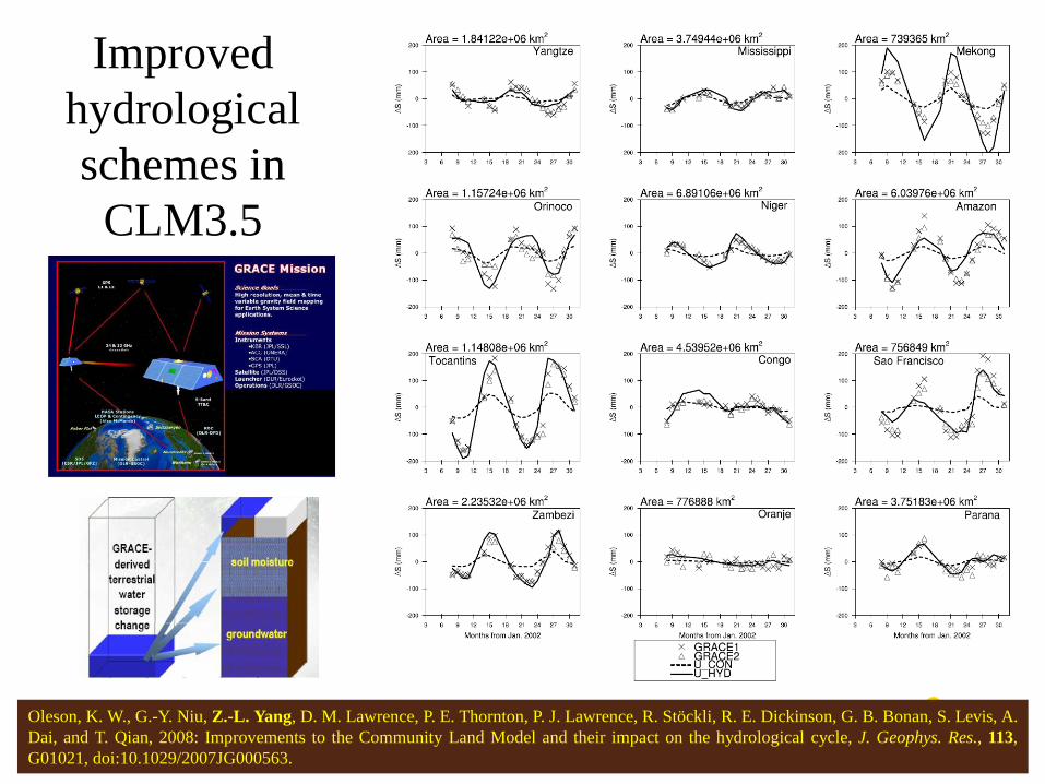
Improved

hydrological

schemes in

CLM3.5

Oleson, K. W., G.-Y. Niu, Z.-L. Yang, D. M. Lawrence, P. E. Thornton, P. J. Lawrence, R. Stöckli, R. E. Dickinson, G. B. Bonan, S. Levis, A.

Dai, and T. Qian, 2008: Improvements to the Community Land Model and their impact on the hydrological cycle, J. Geophys. Res., 113,

G01021, doi:10.1029/2007JG000563.

ang

56

Improving Interception, Runoff, and Frozen Soil

Process in CLM2

Niu and Yang, 2006, GRL

ang

Terrestrial Water Storage Change

GRACE (MAM – SON)

CCSM4 (MAM – SON) (Fully coupled global land, atmosphere,

ocean, ice climate model)

CCSM3 (MAM – SON)

Gent et al., 2011

ang

58

Noah Land Surface Model

ang

A Simple Groundwater Model (SIMGM)

bot

botbota

zz

zzKQ

)(

Water storage in an unconfined aquifer:

)1(bot

bota

zzK

sba RQ

dt

dW ya SWz /

Recharge Rate:

Modified to consider macropore effects: Cmic * ψbot Cmic fraction of micropore content

0.0 – 1.0 (0.0 ~ free drainage)

Niu, Yang et al. (2011)

ang

Micropore fraction: Cmic = 0.5

A Simple Groundwater Model

(SIMGM)

ang

Does including dynamic vegetation phenology and

water table in a climate model improve seasonal

precipitation forecasts?

ang

Vegetation growth

Sunlight

CO2

Oxygen

Soil moisture

Stomata

Evapotranspiration

ang

Modeling Vegetation Phenology (Dickinson et al., 1998)

Carbon

assimilation

Stomatal

Resistance

ang

Groundwater System

http://ga.water.usgs.gov/edu/graphics/wcgwdischarge.jpg

ang

Modeling Groundwater in Climate Models (Niu et al., 2007)

ang

66

WRF Simulated & Observed Monthly and Seasonal Mean

Precipitation in Central Great Plains

The WRF model with a dynamic vegetation growth (DV) improves, over the DEFAULT, the rainfall simulation in Central Great Plains in the USA, i.e., the transition zones between arid/semi-arid and humid regions, especially in July, August, and the entire summertime (JJA).

Further consideration of the dynamic water table (DVGW) improves the simulation even more.

These improvements are due to the improved coupling between soil moisture and precipitation through lowered lifting condensation level (see next slide).

This study suggests incorporating vegetation and groundwater dynamics into a regional climate model would be beneficial for seasonal precipitation forecast in the transition zones.

Jiang, X., G.-Y. Niu, and Z.-L. Yang, 2009: Impacts of vegetation and groundwater dynamics on warm season precipitation

over the Central United States, J. Geophys. Res., 114, D06109, doi:10.1029/2008JD010756.

ang

Lifting condensation level (LCL) height versus soil

moisture index (SMI) in the soil layers

Jiang, X., G.-Y. Niu, and Z.-L. Yang, 2009: Impacts of vegetation and groundwater dynamics on warm

season precipitation over the Central United States, J. Geophys. Res., 114, D06109,

doi:10.1029/2008JD010756.

ang

Noah LSM with multi-physics options

1. Leaf area index (prescribed; predicted) 2. Turbulent transfer (Noah; NCAR LSM) 3. Soil moisture stress factor for transpiration (Noah; BATS; CLM) 4. Canopy stomatal resistance (Jarvis; Ball-Berry) 5. Snow surface albedo (BATS; CLASS) 6. Frozen soil permeability (Noah; Niu and Yang, 2006) 7. Supercooled liquid water (Noah; Niu and Yang, 2006) 8. Radiation transfer: Modified two-stream: Gap = F (3D structure; solar zenith angle;

...) ≤ 1-GVF Two-stream applied to the entire grid cell: Gap = 0 Two-stream applied to fractional vegetated area: Gap = 1-GVF 9. Partitioning of precipitation to snowfall and rainfall (CLM; Noah) 10. Runoff and groundwater: TOPMODEL with groundwater TOPMODEL with an equilibrium water table (Chen&Kumar,2001) Original Noah scheme BATS surface runoff and free drainage More to be added

Niu, Yang, et al. (2011)

Collaborators: UT, NCAR, NCEP/NOAA, and others

ang

Maximum # of Combinations 1. Leaf area index (prescribed; predicted) 2 2. Turbulent transfer (Noah; NCAR LSM) 2 3. Soil moisture stress factor for transp. (Noah; BATS; CLM) 3 4. Canopy stomatal resistance (Jarvis; Ball-Berry) 2 5. Snow surface albedo (BATS; CLASS) 2 6. Frozen soil permeability (Noah; Niu and Yang, 2006) 2 7. Supercooled liquid water (Noah; Niu and Yang, 2006) 2 8. Radiation transfer: 3 Modified two-stream: Gap = F (3D structure; solar zenith angle;

...) ≤ 1-GVF Two-stream applied to the entire grid cell: Gap = 0 Two-stream applied to fractional vegetated area: Gap = 1-GVF 9. Partitioning of precipitation to snow- and rainfall (CLM; Noah) 2 10. Runoff and groundwater: 4 TOPMODEL with groundwater TOPMODEL with an equilibrium water table (Chen&Kumar,2001) Original Noah scheme BATS surface runoff and free drainage

2x2x3x2x2x2x2x3x2x4 = 4608 combinations

Process understanding, probabilistic forecasting, quantifying uncertainties

ang

70

36 Ensemble Experiments

ang

71

36 Ensemble Experiments

1. Runoff scheme is shown as the dominant player in the SM-ET relationship: SIMTOP (bottom sealed; green) produces the wettest soil and greatest ET; BATS (greatest surface runoff: grey) produces the driest soil and smallest ET.

2. Runoff scheme plays as a provider of soil water (besides precipitation) while surface schemes plays as a “consumer” of soil water.

ang

Traditionally, land surface modeling

• treats land as a lower boundary condition in weather and climate models;

• determines the coupling strength and land–atmosphere interactions and feedbacks;

• calculates, in both coupled and offline modes, evapotranspiration (ET), other fluxes (sensible heat, reflected solar radiation , upward longwave radiation, runoff), and state variables (soil moisture, snow water equivalent, soil temperature).

Driven by IPCC and hydrologic/environmental applications, land surface models

• have evolved greatly in the past three decades;

• are becoming more complex as we are facing the emerging need to – understand climate variability and change on all time/space scales,

– quantify the climatic impacts on energy/water resources and environmental conditions for decision making.

• demand cross-cutting efforts from multi-disciplinary groups.

Summary

ang

Thank you!

Prof. Zong-Liang Yang

+1-512-471-3824

[email protected]

http://www.geo.utexas.edu/climate

Major References

Yang, Z.-L., 2004: Modeling land surface processes in short-term weather and climate studies, in Observations, Theory, and

Modeling of Atmospheric Variability, (ed. X. Zhu), World Scientific Series on Meteorology of East Asia, Vol. 3, World Scientific

Publishing Corporation, Singapore, 288-313.

Yang, Z.-L., 2008: Description of recent snow models, in Snow and Climate, Edited by R. L. Armstrong and E. Martin, Cambridge

University Press, 129-136.

Yang, Z.-L., 2010: Global Land Atmosphere Interaction Dynamics, Graduate Course, The University of Texas at Austin,

http://www.geo.utexas.edu/courses/387H/SyllabusLAID.htm

Other citations can be found at http://www.geo.utexas.edu/climate/recent_publications.html














Land Surface Processes - The Department of Geological Sciences

Documents

Transcript of Land Surface Processes - The Department of Geological Sciences