Land and Construction Economics - Advanced Investment Appraisal

The lecture notes on this component can be downloaded from the web page : http://hkusury2.hku.hk/liin the file : LCE-Notes 01 , under the heading : Notes to BSc. In Surveying Students Year Two

Please Switch Off Your Mobile Phone and Pager as I DO NOT Want to Talk To Your Friends !

The basic logic of the investment method is the understanding that money has a time value. Money receivable in the future is worth less then money of the same amount receivable today.

Investment Valuation

Hence, the present value (PV) of one dollar receivable after n years at an interest rate (or discount rate) of i is worth :

The product of formula can be called a PV factor. This is a factor for this can be multiplied to any future value of a fixed sum (as opposed to a stream of future values in the case of years’ purchase factor, discussed later) of money to find the present value.

The PV factor is always less than 1 because future value is always less than present value in real terms. The reasons for this are mainly twofold. One is the opportunity cost in expecting future value. Opportunity cost is the return forgone in other investment opportunities when investing in a particular project.

PVi n

1

1( )

For instance, if an investor has HK$100 and he invests all of this sum into project A, the opportunity cost for this decision is the likely return he could have achieved from projects B,C or D had he chosen to do so. So long as project A compensates him enough or opportunity cost is less than return from project A, the investment is a sound one. In the present value situation, the utility of immediate consumption is always greater than deferred consumption. Hence future value is less than present value.

The second reason is the age of inflation. Future value is always readily eroded by inflation in terms of purchasing power.

In fact, the PV factor formula can be analyzed from reverse in an investment angle. For instance, if we have HK$100 today and invest this sum into a regular investment giving a 10% return per annum.

In one year’s time, we will have HK$110 (since HK$100 x (1+10%) = HK$110). In this case, 10% is our required rate of return.

Now, let’s look at this from the future. If we are given an opportunity to receive HK$110 in one year’s time, how much are we prepare to pay for such opportunity ? Since we can earn 10% from a regular investment, we will use 10% as the discount rate to find the present value. As a result, the present value of HK$110 in a year’s time is :HK$110 x 1/(1+10%) = HK$100. This illustrates the fact that the discount rate and rate of return for investment are closely related. To a certain extent, we can even assert that they are the same.

When the value of the stream of incomes (I) is fixed within the holding period, the capital value (V) of the interest in property (hence the summation of the future incomes) during the holding period then becomes :

It is also obvious that when the holding period approaches infinity, the re-sale value of the asset approaches zero, hence it becomes relatively insignificant. In infinity, PV of the reversionary capital value approaches 0 such that formula becomes :

VPV

iI

1*

VI

i

Suppose a property whose rental income per annum is HK$ 20. This amount is fixed and unchanged forever. Assuming rental income is receivable at the end of each year, and our required rate of return for property is 20%, we’ll be able to find out the value of this property by formula. Since the property is for rental forever, there is no reversionary sale price, formula becomes :

Assume year 1000 is a proxy for eternity, the summation incomes is HK$100. This is obtained either through the serial calculation or just : HK$20/20% = HK$100.

$20

(

$20

(

$20

(....

$20

($100

1 20%) 1 20%) 1 20%) 1 20%)2 3 1000

In any case, we can prove that if we pay HK$100 today, and getting HK$20 per year, it is an investment with return of 20% p.a.( i.e. return or yield is equal to annual income divided by capital value). This exactly reflects what we require before the valuation process.

Now, let’s assume a more realistic situation that rental does grow as time goes by. Assuming a 12% rental growth per year due to an upsurge of demand for this kind of property,

$20

(

$22.

(

$25

(....

$20( .

($250

1 20%)

4

1 20%) 1 20%)

1 12%)

1 20%)2 3

1000

1000

If we are patient enough, we can try to add up all these together and V will turn out to be HK$ 250. In this case, the yield has dropped to : HK$20/HK$250 = 8% ! Superficially, it does not make sense. Logically, when there is an increase in demand leading to a rise in rental income, the rate of return should increase as well ! In fact, the opposite happens. This is the case even when we assume that the increase in rental value starts immediately so that it becomes :

$22.

(

$25

(

$28

(....

$20( .

($280

4

1 20%) 1 20%) 1 20%)

1 12%)

1 20%)2 3

1000

1000

In this case, V becomes HK$280 but yield remains 8% (i.e. HK$22.4/HK$280 = 0.08).

When there is future growth in the rental income, a new definition of yield is spinned off from the general concept of the rate of return.

In fact, in both cases, we are not getting less than 20% p.a. This is because in both cases, we are using 20%, the required

rate of return to discount future values. What is different is the initial yield we are getting. As the initial income of HK$20 or HK$22.4 represents the

initial rental level only with an implication that in the future, this level will go up at a rate of about 12% p.a.

As a result, we are willing to accept a yield initially lower than what we require in the understanding that the rental income we are getting from this property will go up in the future.

Since the definition of yield is always income divided by capital value.

When there is future growth in the rental level, the initial rental income is always lower than the future rental level.

Hence, the initial yield will be lower than the expected rate of return.

In addition, there is a hidden relationship in both cases. In these two cases, we have a required rate of return of 20% p.a. and a rental growth rate of 12% p.a.

When we deduct the rental growth rate from the rate of return, it becomes 8%, which is equal to the initial yield ! As a result, initial yield may be applied to future inflated income etc.

Discount Rate :

1) Weighted Average Cost of Capital (WACC). Damodaran (1996) defines WACC as the weighted average of the costs of the different components of financing used by a firm. He gives the following formula for the WACC as :

WACC = ke(E/[E+D+PS])+kd(D/[E+D+PS])+kps(PS/[E+D+PS])

Where : ke = cost of equity

kd = after-tax cost of debt

kps = cost of preferred stock

E/[E+D+PS] = market value proportion of equity in funding mix

D/[E+D+PS] = market value proportion of debt in funding mix

PS/[E+D+PS] = market value proportion of preferred stock in funding mix, if any*

* In some cases, this component does not exist

2)Dividend Discount Model : DDM In the simplest case, discount rate is equal to cap. Rate

plus growth rate :Case 1 :Value : $10,000,000 Initial rental : $700,000Growth rate : 4%Holding period : 5 yearsDisposal cap. Rate : 7%

Year 1 Year 2 Year 3 Year 4Year 5

700,000 728,000 757,120787,405 818,901

PV@11% 0.9009 0.8116 0.73120.6587 0.5935

P.V. 630,631 590,861 553,600518,688 485,978

Disposal Value :Expected Year 6 Rental : $851,657Cap. Rate : 7%

PV. @ 11% 0.5935 Equals : 7,220,243

Hence, the value of this real estate is :PV of :

Year One Rental : 630,631Year Two Rental : 590,861Year Three Rental : 553,600Year Four Rental : 518,688Year Five Rental : 485,978Year Six Disposal Value: 7,220,243 Total : $10,000,000

Case 2 :Value :

$10,000,000 Initial rental :

$900,000Growth rate : 3%Holding period : 5 yearsDisposal cap. Rate : 9%

Year 1 Year 2 Year 3 Year 4Year 5

900,000 727,000 954,810983,454 1,012,958

PV@12% 0.8929 0.7972 0.71180.6355 0.5674

P.V. 803,571 738,999 679,615625,003 574,780

Disposal Value :Expected Year 6 Rental : $1,043,347Cap. Rate : 9%PV. @ 12% 0.55674 Equals : 6,578,032

Hence, the value of this real estate is :PV of :Year One Rental : 803,571Year Two Rental : 738,999Year Three Rental : 679,615Year Four Rental : 625,003Year Five Rental : 574,780Year Six Disposal Value: 6,578,032 Total : $10,000,000

The Capital Asset Pricing Model (CAPM) evolved from stock market valuation in mid-60’s.

In the simplest and non-mathematical terminology, CAPM states that an asset’s expected return, which has included the basis of a risk free return, is a positive and linear function of its correlation (in the form of covariance) of returns with a portfolio of all other risk assets available in the market.

The risk free return is normally referred to as the government bond or debenture rate. In the stock market, it has been widely used to apply in the estimation of the performance of stock, in terms of rate of return. Basically, the model states that the expected return of any asset is :

Expected return = risk free return plus risk premium

For the estimation of risk premium, a Beta value is required to be estimated which shows the covariance of the asset with the general market return.

Again, in the simplest wording, the risk premium is the market risk factor of the asset multiplied by the difference between the general market expected return and the risk free return.

Due to the theoretical attractiveness of the model and the general lack of other models in estimating rate of return for real estate, there has been a growth interest in the application of this model in the property market.

In 1984, Gerald Brown carried out an empirical test for this model using market returns in the U.K. , Brown tried to estimate the expected returns for various property sectors.

According to his findings, the return on long-date gilts at that time was 11% while the general broaaly-based market return was estimated to be 20%.

In addition, he calculated that the Beta value for property, hence the estimation of market risk for property was 0.2. Using a CAPM model, the expected return for property in general was :

11% + 0.2(20% - 11%) = 12.8%

In his next step, he estimated the market risk of each sub-sector in the property market relative to the property market as a whole.

He did this by carrying out a regression analysis on the returns of each sectors against the general property market returns.

When this was done, he found the Beta values for each sub-sector and when these Beta values were multiplied by the Beta value of the property market as a whole, he further deduced the risk of each sub-sector relative to the whole investment market as follows :

Retail 1.16 1.16 x 0.2 = 0.23 Office 0.87 0.87 x 0.2 = 0.17 Industrial 0.69 0.69 x 0.2 = 0.14

Accordingly, the expected returns for each of these sub-sectors can now be deduced as follows :

Retail = 11% + 0.23 ( 20% - 11%) = 13.07% Office = 11% + 0.17 ( 20% - 11%) = 12.53% Industrial = 11% + 0.14 ( 20% - 11%) =

12.26%

Nevertheless, due to the fundamental differences between the property market and other capital markets, the application of CAPM in the property market emerged only recently and is still in the trial stage.

Such differences include the availability of market data due to the lack of a central clearing house similar to a central stock exchange for real estate; the heterogeneous nature each property and the indivisibility of real estate.

The traditional approach of investment method of valuation tends to rely on initial income and the market yield to carry out capitalisation process.

The market property yield, which is commonly derived from the relationship between the current open market rent and the current market value of similar properties, has itself carried an implication of future rental growth potential (or diminution).

This is because the open market rent at any time represents the maximum initial rental receivable.

Under most of the circumstances, rental value will vary with the economic environment and the property market sentiment.

If we take a very long span of time, say 50 years, rental value should have a positive growth rate per year, on average.

This is the point which most valuers will find puzzled when trying to adopt a suitable discount rate for future incomes. Traditional text books teach us that it is the market property yield that should be used in the capitalisation process, regardless of the implications of the future incomes.

A more reasonable in adopting the rate is to look at the potential movement of these future incomes.

If the capitalisation process takes into account of the current market rent only, then the current market yield should be used. Where we are capitalising a stream of fixed future values, the discount rate, taking into account of the expected rate of return, opportunity cost and the risk premium should be used.

The traditional wisdom of using the years’ purchase factor for both eternally receivable incomes and fixed period incomes therefore attracts the problem of this yield choosing criteria.

A relatively simple solution to this yield choosing problem is to turn to discounted cash flow model (D.C.F.) where only the discount rate for future values is to be used.

However, as with other financial analytical techniques, the D.C.F. model is itself not without drawbacks.

Criticisms have been raised by various authorities on different aspects of the model.

These cautious notes include the need to consider the relationship of risk as it applies to the discount rate as opposed to the capitalisation rate in the D.C.F. model, the lack of substantial proof that the use of D.C.F. model actually improves an investor’s performance and the reasonableness in setting the various assumptions in the D.C.F. model.

Nevertheless, compared to the conventional capitalisation process for varying incomes, the D.C.F. model can avoid the problem of defining and justifying the use of market yield in various stages of the valuation.

In a D.C.F. model, the discount rate is simply the required rate of return. What we need to focus on is the rate of compensation for future cash flows at different points of time in the future. Deriving from this, we may even have different discount rates for different stages of future incomes, depending on the risk premium required for each stage of the cash flow.

Furthermore, D.C.F. makes realistic assumption to the valuation, especially on the part of property finance.

If we accept that most property investments are carried out with property finance, or on a mortgage-backed system, the value of this real estate should in fact be composed of two elements in terms of property rights, namely the part that belongs to the equity investor and the part that belongs to the lender, or the bank. Hence, the value of real estate assessed on a mortgage-equity model will be equal to :

equitymortgage VVV

When we further break down these two components, we may see that the value of the mortgage is made up of the total discounted value of the debt service (i.e. total periodic loan repayments made) and the mortgage balance(residual amount of the mortgage loan at the point of re-sale); and the total discounted rental cash flow plus the net equity reversion (net sale proceed to the equity investor after deducting the mortgage balance) receivable at the point of re-sale. Hence :

)(4)(3)(2)(1 nerdsdrcfm VVVVV

Where : V1(m) = mortgaged value of the real estate

V2(drcf) = total discounted rental cashflow

V3(ds) = discounted values of total debt service or re-paid mortgage loan

V4(ner) = net equity reversion, or disposal value minus mortgage balance

Assuming a property will give the following schedule of incomes for the five-year holding period :

Year One HK$120,000 Year Two HK$120,000 Year Three HK$150,000 Year Four HK$150,000 Year Five HK$150,000

In addition to this expected cash flow, the investor expects an average annual capital growth rate of 5% per year. In using a 20% discount rate for his expected rate of return, he is taking out a mortgage from his banker at a mortgage rate of 11.75% p.a. or 0.98% per month for a maximum loan term of 25 years at 70% of the value of the property. He can utilize the above mortgage-equity model to estimate the value of this property by the following steps :

1) V1(m) - mortgaged value of the real estate = 0.7 x V

2) V2(drcf) - total discounted rental cashflow = $402,758.49

3) V3(ds) - discounted values of total debt service =

Mortgaged value times annual mortgage constant times YP factor @ investor’s discount rate :

%20%)201(

11

12

%)98.01(1

1

%98.07.0

5

300

)(1

xxxVxV ds

Hence :

We may notice that if we calculate the annual mortgage constant from the annual mortgage rate instead of the monthly rate, the constant would become 0.125.

VV

xxVxV

ds

ds

26.0

99.212426.07.0

)(1

)(1

V4(ner) - net equity reversion = disposal value minus mortgage balance

Where : mortgage balance at the point of re-sale = This is the ratio annual mortgage constant on the original term

of loan to the annual mortgage constant on the remaining term of loan at the point of re-sale, times the mortgaged value of the real estate :

VV

xVxV

xVxV

mb

mb

mb

67.0108.0

0104.07.0

%)98.01(1

1

%98.0

%)98.01(1

1

%98.07.0

)(

)(

240300

)(

Hence the value of this real estate is :

281.620,258,1$

49.758,402$32.0

49.758,402$068

24.026.049.758,402$7.0

)(4)(3)(2)(1

V

V

VV

VVVV

VVVVV nerdsdrcfm

This can be compared with a less complicated example below using a finance-explicit D.C.F. model incorporated with the above mortgage assumption. By this D.C.F. model, the financial market is more closely and easily linked to the property market.

The value of the property based on this D.C.F. model is assessed at $1,275,915.03. The apparent difference with the above figure of $1,258,620 is due to rounding problem in the computer calculation. We may further analyse the mechanism of this model by looking at the individual components of the model. Option (a) gives the same assumptions as above while option (b) shows that the model is easy to cope with variations in these assumptions. In option (b), rental variation is assumed to be downward adjusted after two years.

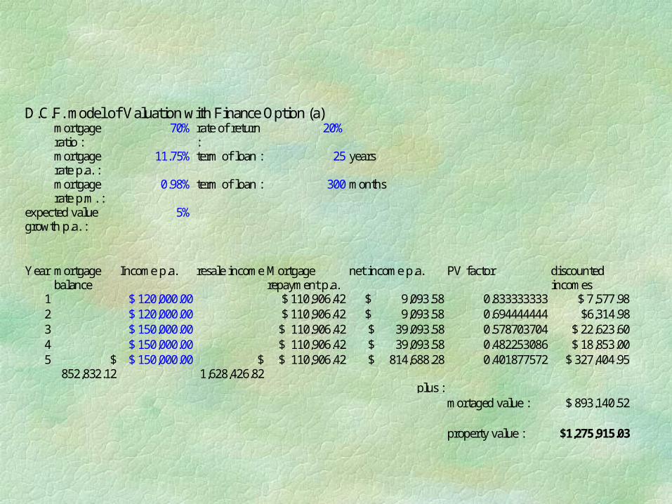
D.C.F. model of Valuation with Finance Option (a)mortgageratio :

70% rate of return:

20%

mortgagerate p.a. :

11.75% term of loan : 25 years

mortgagerate p.m. :

0.98% term of loan : 300 months

expected valuegrowth p.a. :

5%

Year mortgagebalance

Income p.a. resale income Mortgagerepayment p.a.

net income p.a. PV factor discountedincomes

1 $ 120,000.00 $ 110,906.42 $ 9,093.58 0.833333333 $ 7,577.982 $ 120,000.00 $ 110,906.42 $ 9,093.58 0.694444444 $6,314.983 $ 150,000.00 $ 110,906.42 $ 39,093.58 0.578703704 $ 22,623.604 $ 150,000.00 $ 110,906.42 $ 39,093.58 0.482253086 $ 18,853.005 $

852,832.12 $ 150,000.00 $

1,628,426.82 $ 110,906.42 $ 814,688.28 0.401877572 $ 327,404.95

plus :mortaged value : $ 893,140.52

property value : $1,275,915.03

D.C.F. model of Valuation with Finance Option (b)mortgageratio :

70% rate of return : 20%

mortgagerate p.a. :

11.75% term of loan : 25 years

mortgagerate p.m. :

0.98% term of loan : 300 months

expected valuegrowth p.a. :

5%

Year mortgagebalance

Income p.a. resale income Mortgage repaymentp.a.

net incomep.a.

PV factor discountedincomes

1$120,000.00

$84,723.36 $ 35,276.64 0.833333333 $ 29,397.20

2$120,000.00

$ 84,723.36 $ 35,276.64 0.694444444 $ 24,497.67

3 $ 85,000.00 $ 84,723.36 $ 276.64 0.578703704 $ 160.094 $ 85,000.00 $ 84,723.36 $ 276.64 0.482253086 $ 133.415

$651,493.38 $ 85,000.00 $1,243,983.74 $ 84,723.36

$592,767.010.401877572 $ 238,219.76

plus :mortagedvalue :

$682,285.67

propertyvalue :

$ 974,693.81