15ICE-0100/2015-01-2141

Lagrangian Trajectory Simulation of Rotating Regular Shaped IceParticles

Markus WidhalmDLR Braunschweig

Lilienthalplatz 738108 Braunschweig

markus.widhalm@dlr.de

Abstract

This paper focuses on the numerical simulation of the mo-tion of regular shaped ice particles under the forces andtorques generated by aerodynamic loading. Ice particlescan occur during landing and take-off of aircraft at groundlevel up to the lower bound of the stratosphere at cruis-ing altitude. It may be expected that the particle Reynoldsnumber is high because the flow around the aircraft is incertain regions characterized by strong acceleration anddeceleration of the flow. In combination with this flow pat-tern, the rotation of particles becomes important. Applica-ble translational and rotational equations of motion com-bined with a drag correlation taking into account rotationwill be derived for a Lagrangian type particle tracking. Ori-entation is described with quaternions to prevent the sin-gularities associated with the description by Euler angles.The influence of regular shaped particles on collection ef-ficiencies is investigated. Test cases are the flow past acylinder, a NACA0012 airfoil and a NHLP L1/T2 three el-ement airfoil. Due to the increased computational effortcompared to the purely translational approach, observedtrajectory simulation times are reported.

Nomenclature

Variables

A = surface or projected area, m2

CD = aerodynamic drag coefficientCL = aerodynamic lift coefficientd = diameter, m~F = force vector, NI = moment of inertia tensor, kgm2

L = length of particle, mm = mass, kgMa∞ = freestream Mach numberR = rotation matrixRe = Reynolds numberSp = Spin number~T = torque vector, Nmt = physical time, s~x = position vector, components x, y and z, m

Greek lettersα = incidence angleβ = collection efficiency~ϕ = rotation vector, components φ, θ and ψΦ = sphericityΦ⊥ = crosswise sphericityΦ‖ = lengthwise sphericityω = angular velocity, 1/s

Subscripts

p = particle statef = surrounding fluid stater = resistanceR = rotationc.p. = center of pressurec.g. = center of gravity∞ = freestream stateref = reference staterel = relative state

Introduction

Ice crystals may be found at the upper boundary of thetroposphere where strong winds exist and jet aircraft fly atcruising speed in the transonic flow regime and high flowReynolds number. Ice crystals found in this part of theatmosphere deviate considerably in shape from spheresand may appear as thin needles up to disc-shaped struc-tures. As the particle size grows from a few micronsto several hundreds of microns a high particle Reynoldsnumber is to be expected as well. These conditions willmost likely cause an arbitrary rotation and orientation ofthe particle around its principal axes.However, as drag is the most important force contribu-tion, early investigations focused on the drag coefficientsof spheres moving through a fluid with relatively low flowand particle Reynolds numbers. By a combination of the-oretical work and extensive experimental testing a hugeamount of data was collected. It resulted in an empiricalcorrelation of the drag coefficient, dependent on the par-ticle Reynolds number. Extension of these correlations to

Page 1 of 15

irregular shaped particles happened in small steps. Ini-tially, a limited number of regular shaped particles wasconsidered by determining the settling behavior and keep-ing track of the free-falling velocity and drag. Many ofthese investigations have been carried out with prisms,cylinders, cones or plates. Again, empirical drag correla-tions were proposed with an additional parameter, oftenreferred to as sphericity. Sphericity is the ratio between acertain characteristic description (e.g. the cross section)of the equivalent sphere and the non-spherical particle.By definition, sphericity does not account for the orienta-tion of the particle in relation to the direction of fluid flow.The main outcome was an increased drag coefficient fornon-spherical particles in comparison to spherical parti-cles. For years, averaged or stochastic correlation wereused to determine drag coefficients based on huge setsof experimental data for different, mostly regular shaped,particles [1, 2, 3] and have been extended to irregularshaped particles to provide a reliable drag correlation thatcovers as many shapes as possible. The computationaleffort to evaluate the drag coefficient will be comparableto spherical particles.However, if the particle Reynolds number increases con-siderably and experimental investigations become diffi-cult, considering the full particle motion including rotationmay significantly enhance the trajectory simulation. Oneof the first investigations was done by Jeffery [4] for ellip-soids and by Cox [5] for slender bodies, both comprehen-sive theoretical studies. The influence of particle rotationat higher particle Reynolds numbers was recently pointedout by Qi [6] while investigating sedimentation. Huanget.al. [7] identified different modes of particle motion re-lated to a wide range of particle Reynolds numbers forspheroidal particles in a Couette flow. Rosendahl [8] in-troduced a multi-parameter description of the particle ro-tation to improve prediction capability of numerical sim-ulations instead of using a general single parameter likethe sphericity. Comprehensive overview article on exten-sions to more general regular and irregular shaped parti-cles may be found in Loth [9], Mandø and Rosendahl [10]and Kleinstreuer and Feng [11]. Experimental investiga-tions of rotating balls in a turbulent flow were examined byZimmermann et. al. [12].Obviously, the general treatment of non-spherical parti-cles needs to consider the shape and orientation depen-dent aerodynamic forces, which are associated with non-spherical particles. The computation of both the aerody-namic forces and torques and of the particle motion re-quires the tracking of the particle orientation and rotationplus the formulation of appropriate orientation dependentlift and drag correlations. If the translational and rotationalequations of motion are applied, a set of ordinary differ-ential equations emerges, which introduce external forcesand torques. To simplify evaluation of forces and torques,we delimit our investigation in this paper to the treatment

of regular shaped particles only. The forces and torquesmay then be evaluated using orientation based geometri-cal parameters. Certain parameters are derived from ex-periments to keep the computational effort within bounds.

The original DLR TAU Lagrangian-type particle tracer, asdescribed in [13], could only consider translational mo-tion of particles. The equations of motion are derivedfrom Newton’s second law for a point mass, but con-sider drag, buoyancy and gravity forces. The drag cor-relation implemented is based on a fit to Langmuir andBlodgett’s [14] drag data for spherical water droplets ina dispersed flow. The particle tracer was mainly estab-lished to evaluate water droplet collection efficiencies forsubsequent ice accretion simulations. The resulting ordi-nary differential equation (ODE) is solved in time with em-bedded Runge-Kutta methods of third or fourth order. Anextension to the original implementation, solving in addi-tion the rotational equations of motion and the equationsfor evaluating the orientation, is described in this paper.As irregular shapes are difficult to treat and the accurateaerodynamics around the particle surface is not resolvedin our approach, restriction to regular shaped particles arenecessary. We consider both discs and rods with speci-fied aspect ratios, for which the equation of motion canbe derived by basic mechanical considerations since ex-perimental data are rare. Aerodynamic forces and cor-responding torques are introduced from existing correla-tions which account for orientation and non-spherical pa-rameters.

A suitable drag correlation approach was introduced byHölzer and Sommerfeld [15], which depends on the parti-cle Reynolds number, lengthwise and crosswise spheric-ity and a general description of the sphericity. Lift andresistance torque against the rotation is treated as pro-posed by Mandø and Rosendahl [10]. Computation ofparticle orientation angles and angular velocity is done inthe principal axis system of the considered particle usingEuler’s equations for a rotational motion. Orientation isrepresented using quaternions. However, the quaternionrepresentation needs to be transferred back into Euler an-gles to recompute projected areas and equivalent sphereparameters. The differential equations for rotational andthe translational motion based on Newton’s law form to-gether a system of ordinary differential equations, whichis again solved in time by embedded Runge-Kutta integra-tors with local error control. The demand of this solutionprocess on computer time is outlined too, which is a lim-iting factor for the potential use in industrial applications,whenever orientation of particles is considered. Evalu-ation of collection efficiencies for selected test cases willemphasize the influence of particle rotation in comparisonto averaged correlation approaches.

Page 2 of 15

Governing equations of particle mo-tion

The governing equations for the translational and rota-tional motion of a particle in a fluid is Newton’s secondlaw in a global frame of reference,

~xp(t) := [xp(t), yp(t), zp(t)]T , (1)

d~xp(t)

dt:= ~xp(t) = ~Up(t), (2)

mpd~Up(t)

dt:=∑

~F (t), (3)

and Euler’s equations of motion in a body fixed frame ofreference

~ϕp(t) := [φ(t), θ(t), ψ(t)]T , (4)d~ϕp(t)

dt:= ~ϕp(t) = ~ωp(t), (5)

Ipd~ωp(t)

dt+ ~ωp(t)× (Ip~ωp(t)) :=

∑~T (t), (6)

Ip :=

Ixx Ixy IxzIyx Iyy IyzIzx Izy Izz

(7)

where mp is the particle mass and Ip is the particle’s mo-ments of inertia tensor, respectively. Both are kept con-stant. In the present paper, the index p denotes a parti-cle property whereas index f is used for properties of thesurrounding fluid. Furthermore, Figure 1 shows the bodyfixed coordinate system [x, y, z] and the geodesic refer-ence coordinate system [xg, yg, zg].

L2

c.g. ωp − ωfUf

x

z

zgxg

yg

FL

FD

xcp

y

α

d p

c.p.

Figure 1: Aerodynamic forces acting at the center of pres-sure (c.p.) on a slender body and showing the relationshipbetween geodesic [xg, yg, zg] and body fixed [x, y, z] coor-dinate system.

It is not appropriate to solve the Eq. (5) directly with a ro-tation matrix based on Euler angles due to an inherentsingularity, well-known as gimbal lock. It appears when-ever the second rotation turns the first rotation axis paral-lel to the third axis of rotation, and the sequence of rota-tions loses one degree of freedom, [12, 16]. An alternativerepresentation of the orientation, preventing gimbal locks,is a representation by four variables called quaternionsand introduced as generalized coordinates to solve theequations of rotation. After choosing an appropriate Eulerrotation sequence (3-1-3), described in [17], the quater-nion parameters q(t) ∈ R4 and q := q(t) are defined as,[18, 17],

q := [q0, (q1, q2, q3)]T , (8)

q0 := cosθ

2cos

(φ+ ψ

2

), (9)

q1 := sinθ

2cos

(φ− ψ

2

), (10)

q2 := sinθ

2sin

(φ− ψ

2

), (11)

q3 := cosθ

2sin

(φ+ ψ

2

)(12)

The angular velocity transformation matrix from a body-fixed frame of reference to a geodesic frame of referenceand vice versa can be written as

~ωgp := q ∧ ~ωp ∧ q, (13)

~ωp := q ∧ ~ωgp ∧ q (14)

where q denotes the conjugate quaternion, q ∧ q ≡ 1 ifthe quaternion is normalized to 1 and ∧ is the Grassmannproduct. Defining the product of Eq. (13) is a matter ofconvention, since it changes the effect of rotation direc-tion. Eq. (13) results in a clockwise rotation.Switching from quaternion to a matrix notation leads tothe following alternative formulation

~ωgp := R(q)~ω, ~ωp := RT (q)~ωgp . (15)

Since for a unit quaternion the following equivalence holdsR−1(q) ≡ RT (q) ≡ R(q), the orthogonal rotation matrixR(q) is then defined by

R(q) =

r11 r12 r13

r21 r22 r23

r31 r32 r33

=

=

12 − q2

2 − q23 q3q0 − q2q1 q1q3 + q2q0

−(q2q1 + q3q0) 12 − q2

1 − q23 q0q1 − q2q3

q1q3 − q2q0 −(q2q3 + q1q0) 12 − q2

1 − q22

(16)

The implementation ofR(q) is introduced as 2R(q) to savethe multiplication of Eq. (17) by 0.5. The equation of state

Page 3 of 15

variables for each particle satisfies the equation

q =1

2(~ωgp ∧ q) =

1

2(q ∧ ~ωp) =

1

2Q(q)

[0~ωp

](17)

Q(q) =

q0 −q1 −q2 −q3

q1 q0 q3 −q2

q2 −q3 q0 q1

q3 q2 −q1 q0

(18)

An equation defining the second derivative of q, q :=q(q(t), ωp(t)), is obtained by differentiating Eq. (17). Thisresults in a second-order ODE for q,

q =1

2(q ∧ ~ωp + q ∧ ~ωp), ~ωp = 2(q ∧ q) (19)

q =1

2

[|q|0

]+

1

2(q ∧ ~ωp) =

1

2Q(q)

[0

~ωp

](20)

Transformation from quaternions back to Euler angles isprovided with the rotation matrix in Euler angles

R313(~ϕp) =

cφcψ − sφcθsψ cψsφ + cφcθsψ sψsθ−sφcψ − sφcθcψ −sφsψ + cφcθcψ cψsθ

sθsφ −sθcφ cθ

(21)

sϕ := sin(ϕ), cϕ := cos(ϕ).

(22)

Equivalent to matrix R(q), Eq (16), the Euler angles aredefined by

~ϕp(R(q)) :=

arctan 2(r31,−r32)arccos(r33)

arctan 2(r13, r23)

(23)

which is used for computing projected areas and the angleof attack of the fluid. Note, that arccos of ±1 is not defined.The arccos function returns the angle between 0 and πradians. The singularities are identified with Eq. (21) asr33 = −1→ π radians and r33 = 1→ 0 radians.A common problem in the integration of rotational motionsdescribed by quaternions is the inherent quaternion drift.The quaternion is defined as a unit quaternion and itslength has to remain equal to one. However, during inte-gration the quaternions will drift away from this unit length.Therefore, it is necessary to re-normalize the quaternionsat an appropriate time.

qnew =q

|q| , |q| =√q20 + q2

1 + q22 + q2

3 (24)

During the particle simulation the normalization was per-formed after each completed time step.Finally, solving the equation for the particle angular veloc-ity, Eq. (6) and Eq. (17) may be rewritten as

~ωp = I−1p

(~T − ~ωp × (Ip~ωp)

)(25)

Introducing a reference moment of inertia, the momentsof inertia may be non-dimensionalized

Iref,p = ρp d5p, I

′

p =IpIref,p

(26)

which equates for spheres and cylinders to

I′

p,sphere =π

60(27)

I′

p,x,cyl =π

32c, I

′

p,y,z,cyl =1

48c(

3

4+ c2) (28)

the dimensionless angular acceleration yields

~ω′

p = (I′

p)−1(~T

′ − ~ω′

p × (I′

p~ω′

p))

(29)

~ω′

p = ~ωpLref

xref(30)

xref equals the magnitude of the free stream velocity andLref is the characteristic length of the airfoil, e.g. the chordlength. These are equations for the translational and an-gular acceleration and the quaternion. It represents asystem of 10 differential equations to be solved insteadof 3 differential equations to be solved for the basic La-grangian trajectory simulation. The equations are inte-grated in time numerically with an embedded fourth-orderRunge-Kutta method.

Forces and Torques

The sum of all forces in Eq. (3) acting on the particle mayconsist of the aerodynamic lift and drag and forces result-ing from the density difference between particle and fluid(buoyancy and gravity),∑

~F = ~FDrag + ~FLift + ~FBuoyancy + ~FGravity + · · · . (31)

All other forces are neglected. Introducing the relative ve-locity between particle and fluid ~xrel = ~xp − ~xf and usinga drag law, where the drag varies with the relative velocitysquared, Eq.(3) may be written

~xp = (−CD + CLR(q⊥))Ap,Sρf

2mp|~xrel|~xrel −

ρfρp~g + ~g, (32)

q⊥ :=(π

2,~arot

)→ R(q⊥), (33)

~arot :=

if ~xrel·~z|~xrel·~z|

= 1 then [0,−1, 0]T ,

if ~xrel·~z|~xrel·~z|

= −1 then [0, 1, 0]T ,

else ~xrel×~z|~xrel×~z|

(34)

where Ap,S , ρp, mp and CD are the cross section of theequivalent sphere, the particle density, the mass and thedrag coefficient of the particle, respectively. ρf is the den-sity of the fluid. ~g is the gravity vector. The drag force

Page 4 of 15

is negative parallel and the lift force acts perpendicularto the relative velocity vector. The orientation of the liftforce can be established by applying a Householder trans-formation, arbitrary axis is chosen to be the body fixed~z := [0, 0, 1]T axis, and conversion into a quaternion toevaluate the rotation matrix R(q⊥).By rearranging the equation above, Eq. (34) may be ex-pressed as

~xp = (−CD + CLR(q⊥))Rep24

18

d2p

µfρp~xrel +

ρp − ρfρp

~g. (35)

with dp, the particle diameter, and Rep, the particleReynolds number, defined as

Rep =|~xrel| dpρf

µf. (36)

If Eq. (35) is written in dimensionless form (dashed quan-tities are dimensionless),

~x′p = (−CD +CLR(q⊥))Rep24

1

K~x′rel +Fr2 ρp − ρf

ρp

~g

|~g| , (37)

then two similarity parameters of the particle-fluid inter-action become apparent, the so-called inertia parameterK,

K =d2p

18

ρpµf

xref

Lref, (38)

and the Froude number, Fr = xref/√|~g|Lref.

The inertia parameter K is the ratio between a particlerelaxation time and a characteristic time of the fluid flow.The Froude number Fr is the ratio between gravitationalforces and fluid forces.Hölzer and Sommerfeld [15] introduced a drag correlationfor the complete Reynolds number region:

CD :=8

Rep1√Φ‖

+16

Rep1√Φ

+3√Re

1

Φ34

+

+ 0.42 · 100.4(−log(Φ))0.2 1

Φ⊥(39)

which depends on the shape, the orientation and the par-ticle Reynolds number. The sphericity (Φ) representsthe ratio between the surface area of the volume equiv-alent sphere and that of the considered particle. Thecrosswise sphericity (Φ⊥) is the ratio between the cross-sectional area of the volume equivalent sphere and theprojected cross-sectional area of the considered particle.The lengthwise sphericity (Φ‖) is the ratio between thecross-sectional area of the volume equivalent sphere andthe difference between half the surface area and the meanprojected longitudinal cross-sectional area of the consid-ered particle.

[deg]

CD

0 15 30 45 60 75 90

0.8

1

1.2

1.4

SphereCyl. L/d=1.0, H&SCyl. L/d=1.0Cyl. L/d=1.5, H&SCyl. L/d=1.5Disc L/d=0.5

Figure 2: Comparison of the values for drag coefficientextracted from Hölzer and Sommerfeld [19] for cylindricalparticles at Rep = 240 with the implementation in TAU. Inaddition, the drag coefficient for a disc with an aspect ratioof 0.5 is presented.

The drag coefficient for cylindrical particles obtained fromHölzer and Sommerfeld is presented in Figure 2 in com-parison with the implementation of Eq. (39) in TAU for aparticle Reynolds number of 240 for a quarter rotation ofthe particle. Figure 2 includes the drag coefficient for adisc with an aspect ratio of 0.5. A noticeable effect is thehigher drag coefficient for the disc at 90 degrees (flat inflow direction) and the lower coefficient for the cylindricalparticle at 0 degree (cross section in flow direction). Thediameter was kept constant which then scales the lengthor thickness of the particle with the aspect ratio.

To characterize non-spherical objects, Wadell [20] intro-duced the sphericity Φ. It is the ratio of a volumetric equiv-alent surface of a sphere and the actual surface of a par-ticle. The sphericity is defined as

Φ =A0,Sphere

A0:=

d2v

d2A0

, dA0=

√1

πA0, (40)

Φcyl =2(

32c)2/3

1 + 2c, c =

L

dp, dv :=

(6

πVp

)1/3

(41)

Φ will be in the range Φ ≤ 1, with Φ ≡ 1 for a sphere anddv is the equivalent diameter for a sphere of the samevolume. Obviously, the sphericity does not account fororientation of the particle which is evident and was notedalready by Wadell.

Similar to the sphericity, two additional sphericities maybe defined, the crosswise and lengthwise sphericity, re-

Page 5 of 15

spectively,

Φ⊥ :=A⊥,Sphere

A⊥:=

d2v

d2A⊥

, dA⊥ :=

√4

πA⊥ (42)

Φ‖ :=A‖,Sphere12A0 −A‖

:=d2v

2d2A0− d2

A‖

, dA‖ :=

√4

πA‖ (43)

In general the crosswise sphericity is much easier to eval-uate then the lengthwise sphericity. Replacing the length-wise with the crosswise sphericity in the general correla-tion formula Eq. (39) will result in a small relative deviationcompared to the general formula as mentioned by Hölzerand Sommerfeld [15].

[deg]

L/D

L/D

, H

oe

rne

r

0 15 30 45 60 75 900

0.0002

0.0004

0.0006

0.0008

0.001

0

0.05

0.1

0.15

0.2

0.25

0.3

0.35

0.4

0.45

0.5Rep=50

Rep=100

Rep=200

Rep=1000

Hoerner

Figure 3: Lift over drag coefficient ratio from Mandø andRosendahl [10] and Hörner [21] for a quarter rotation ofthe particle.

Lift forces may be differentiated into aerodynamic lift, aris-ing from circulation generated in the fluid flow around theparticles shape, as well as lift due to velocity gradientsin the flow and lift due to particle rotation. The lattertwo are usually called Saffmann and Magnus lift-force, re-spectively. In this paper, aerodynamic lift is consideredonly. Aerodynamic lift may be modelled based on thecross-flow principle of Hörner [21] which relates the aero-dynamic drag coefficient with the lift coefficient by the in-cidence angle

CLCD

= sin2 α cosα, 0 ≤ Rep ≤ 103 (44)

Mandø and Rosendahl [10] modified the ratio betweenlift and drag coefficient to also depend on the particleReynolds number

CLCD

=sin2 α cosα

0.65 + 40Re0.72p

. (45)

Figure 3 compares both approaches. Obviously,Mandø and Rosendahl’s relationship is about three ordersof magnitude smaller than Hörners approach. Due to thatdiscrepancy, Eq. (44) is implemented.The sum of all torques in Eq. (6),∑

~T = ~Tc.p. + ~TR + . . . (46)

are torques around the center of pressure as aerodynamicforces appear and the particles resistance torque againstrotation. All other torques are neglected. Aerodynamicforces act around the center of pressure (c.p.) at thelength xc.p. from the center of gravity. The resulting torqueis

~Tc.p. = ~xc.p. × (Rga ~FD +Rga ~FL) (47)

with the transformation matrix Rga from the aerodynamicinto the geodesic frame. As the particle is not discretizeditself, an adequate description of xc.p., see Figure 1, isextracted from the literature. Rosendahl [8] describes xc.p.as a function of the incidence angle α and the aspect ratioof axes c = L/d

xc.p.L

=1

2(1− exp(1− c)) (1− sin3 α) (48)

and his co-worker Yin [22] proposed a similar relationship

xc.p.L

= 0.25(1− | cos3 α|) (49)

Both distributions are displayed in Figure 4 for a quarterrotation, indicating the orientation of the particle.

[deg]

xc

p/L

0 15 30 45 60 75 900

0.05

0.1

0.15

0.2

0.25Yin

Rosendahl

Figure 4: xc.p./L location during rotation with indication ofthe body’s orientation.

Throughout the simulations Yin’s relationship of xc.p./Lwas preferred.

Page 6 of 15

l

L2

c.g.

ωp − ωf

Fr(l)

Figure 5: Resistance towards rotation [10].

The torque due to resistance can be directly derived by in-tegration of the friction, caused by rotation, over the lengthof the particle, see Figure 5. First the torque will be de-rived with the simplification that the rotation takes placearound the y-axis only, a two-dimensional simplification.The rotational velocity, the Reynolds particle number andthe projected area are defined by

~uR = ~ωrel ×~l, ~ωrel =1

2~ωf − ~ωp (50)

ReR(l) =ρf |~ωrel|dp l

µ, (51)

Ar(l) = d l, (52)

where Ar(l) denotes the projected area towards the par-ticle rotation. White [23] found a drag correlation for cylin-ders in a uniform flow

CD(l) ≈ 1 +10

Re2/3R (l)

, 10−4 < ReR < 2 · 105

which can be integrated analytically. Introducing thatequation for the resistance torque, we obtain for a two-dimensional rotation around the y-axis and introducing theaspect ratio c = L/dp in dimensionless form:

T′

r,y =Tr,yIref,p

(Lref

xref

)2

, (53)

T′

r,y =ρfρp

(ωp,y − ωf,y)2c4L2ref

x2ref

(1

64+

1

3.36Re2/3R

)(54)

Figure 6 points out the rotational torque coefficients for dif-ferent cylindrical shapes using Eq. (54). An analytical ex-pression derived for the rotational torque by Dennis [24],T ′r = 6.84/Re

1/2R + 31/ReR is depicted as well. Note that

Eq. (54) is non-dimensionalized as proposed by Dennis todisplay them accordingly.

Rer

Tr’

10-1 100 101 102 10310-2

10-1

100

101

102

103DennisMando Cyl 1.0Mando Disc 0.5Mando Cyl 2.0

Figure 6: Rotational torque coefficient T ′r as a function ofthe rotational particle Reynolds number for the differentapproaches, Dennis [24] correlation for a sphere is usedas a reference.

A more recent approach for the rotational torque has beenpresented by Zastawny et. al. [25] based on Direct Numer-ical Simulations (DNS) for prolate/oblate spheroids, discsand fibers. The resulting formula is a curve-fit taking intoaccount symmetric and anti-symmetric axis of the parti-cles shape. However, the implementation follows Eq. (54).

Initial conditions

Initialization of the particle’s initial location is providedthrough user input via a single start point, a line of startpositions or a two-dimensional equidistant grid of start po-sitions. After specifying the release location, the particlevelocity is set to the interpolated fluid velocity

~xp

∣∣∣t=0

= ~xf

∣∣∣t=0

. (55)

Regarding rotation, the initial Euler angles ~ϕp are set to[0, π/4, 0]T . Due to the fact that the center of pressurelocation equals zero at θ ≡ 0, an initial value θ 6= 0 has tobe taken. Otherwise no rotation of the particle occurs.Setting the initial particle angular velocity is very difficult,because there is barely any information or experimentaldata available regarding the angular velocity distributionat flight altitudes.In opposition to the numerical modeling of the flow pastan object a uniform flow is assumed at the far field. More-over the rotation of the particle is driven with the torquecaused by aerodynamic forces and the viscous resistanceagainst rotation. However, as the equilibrium torque be-tween aerodynamic and resistance torque in a uniformflow is not known a priori, the particle release location is

Page 7 of 15

well ahead of the obstacle to ensure an almost constantparticle angular velocity.Ice density of ice particles is usually assumed to be 914kg/m3, which corresponds to the ice density of glace ice.

Local collection efficiency

The local collection efficiency β, is the ratio of the areaA0 spanned by four particle release points in the releaseplane projected on to a plane perpendicular to the oncom-ing flow and the area Am spanned by the correspondingparticle impingement points, see Figure 7, and defined by

β =A0 cosα

Am(56)

where α is the angle of attack of the flow. The calculated βvalue is assigned to the centroids (+) of the quadrilaterals.

Figure 7: Determination of local catch efficiency β forthree-dimensional droplet impingement.

Results

It is difficult to validate the correct implementation of theafore-mentioned equations of motion and the physicalcorrectness of the force and torque correlations: Exper-imental data are rare or do not fit to the flow conditionsof interest and DNS simulations can not be performed be-cause of computational cost. However, to gain a certainconfidence in the implementation, Hölzer and Sommer-feld’s drag correlation model has been compared to theoriginal data set, see Figure 2, and the rotational torqueof particles was compared against analytical derived for-mulas, Figure 6. Moreover, to avoid implementation er-rors, for computing the torque generated by aerodynamicforces a procedure is used as a template that has beenalready in use for many years in the TAU code for calcula-tion of airfoil pitching moments.

Therefore, any test case presented in the following is nota validation of the implementation. The test cases onlyserve the purpose to show the appropriateness of a non-rotating particle initial condition and to illustrate the impor-tance of taking into account the rotational motion of par-ticles in certain flow situations. The following test caseshave been considered: The first test case is a poten-tial flow past a cylinder to investigate the developmentof particle rotation for particles released far upstream ofthe cylinder with a zero initial particle angular velocity.The second case is a subsonic laminar flow around aNACA0012 airfoil and the third case is a turbulent flowaround a high-lift device. Both test cases are selected todetermine collection efficiencies on the airfoils comparingrotating cylindrical particles and non-rotating spheres.As it is common to describe the rotation behavior with sim-ilarity parameters, the particle spin number is introducedas follows

Sp =ωpdpUf,∞

(57)

which is in an aerodynamic context the reduced fre-quency. Eq. (57) can be remodeled with the assumption

ωp := ω′pxref

Lref, ω′p = U ′f,∞ ≡ Ma∞ (58)

Sp =U ′f,∞xrefdp

U ′f,∞xrefLref=

dpLref

(59)

where Ma∞ denotes the freestream Mach number. Inparticle related literature, a reference particle diameteris often defined as Lref ≡ dp,ref, mainly for use in non-dimensionalization. Thus, the spin number becomesunity.

Flow past a cylinder

The first test case, a potential flow past a cylinder, hasbeen selected to demonstrate the rotation behavior of par-ticles. The cylindrical body considered has a diameter of0.5 m and a circular far field encompasses the cylinder ata radius of 4.5 m. The flow conditions are summarized inTable 1.

Table 1: Numerical Simulation parameter for theflow past a Cylinder

Ma∞ α [deg.] xref [m/s] dcyl [m] dp[µm]

0.3 0.0 277.4 0.5 100

Cylindrical particles are released very close to the up-stream far field boundary with an initial particle angularvelocity of zero without considering gravity forces. Twotrajectories are considered with different particle aspect

Page 8 of 15

ratios, passing by very close to the top and bottom of thecylinder. The trajectories of the particle with aspect ratioof L/d = 10 can be seen in Figure 8 and for an aspectratio of L/d = 0.1 in Figure 9 as dashed lines. The trajec-tories marked by solid lines, in both figures, are the sameparticles, but without considering rotation, serving as areference. The flow field in both figures is contoured withthe static pressure.

X

Z

-2 -1.5 -1 -0.5 0 0.5 1 1.5 2

-0.5

0

0.5

pressure10.50-0.5-1-1.5-2-2.5-3

Figure 8: Flow past a cylinder at Ma∞=0.3 showing thetrajectory of a cylindrical particle with aspect ratio L/dp =10 (dp = 100µm) without rotation (solid) and with self-induced rotation (dashed).

X

Z

-2 -1.5 -1 -0.5 0 0.5 1 1.5 2

-0.5

0

0.5

pressure10.50-0.5-1-1.5-2-2.5-3

Figure 9: Flow past a cylinder at Ma∞=0.3 showing thetrajectory of a cylindrical particle with aspect ratio L/dp =0.1 (dp = 100µm) without rotation (solid) and with self-induced rotation (dashed).

The upper and lower trajectory between rotating and non-rotating particles with an aspect ratio L/dp = 10 do not dif-fer much as seen in Figure 8. That is related to the overalllow spin of the particles for L/dp > 1 seen in Figure 10and Figure 11. The lifting force and torque will not have agreat impact, except for the drag which remains nearly thesame as for the non-rotating particle. Figure 9 displaysthe upper and lower trajectory for the rotating particle withL/dp = 0.1. It is much more widespread to its non-rotatingcounterpart and they are not symmetric to the z ≡ 0 lineadditionally. First, the deviation to rotating particles withL/dp > 1 is caused by its higher spinning rate while pass-ing the obstacle in comparison to particles with L/dp < 1,resulting in a higher influence of the aerodynamic force.

Second, the non-symmetric behavior between both rotat-ing particle trajectories is related to a negative angle ofattack at the upper trajectory and a positive on the lower,respectively, but the rotation is unaffected by the angle ofattack, see both Figure 10 and Figure 11 for correspond-ing aspect ratios.

x

’ y

­2 ­1 0 1 2

­0.5

0

0.5

1

1.5

2L/d=10L/d=2L/d=1

L/d=0.5L/d=0.1

Sp=1

Figure 10: Dimensionless particle angular velocity mon-itored over covered distance for the trajectories passingthe object above for various aspect ratios L/dp, dp is 100µm.

x

’ y

­2 ­1 0 1 2

­0.5

0

0.5

1

1.5

2L/d=10L/d=2L/d=1

L/d=0.5L/d=0.1

Sp=1

Figure 11: Dimensionless particle angular velocity mon-itored over covered distance for the trajectories passingthe object below for various aspect ratios L/dp, dp is 100µm.

The dimensionless angular velocity of the considered par-ticles are plotted in Figure 10, related to the trajectoriespassing the obstacle above, and Figure 11 is related to

Page 9 of 15

the trajectories passing the obstacle below. Both figuresseem to be the same. The difference in the angular ve-locity for the rotating particles is marginal between thetrajectories passing above or below the obstacle. Thespin of the particle increases naturally when approach-ing towards the obstacle. All particles experience a raisein spin while passing the obstacle and the rotation di-rection is reverted. The spin number of 1 is reached atω′p,y ≡ Ma∞ = 0.3. The particles with higher aspect ra-tio are nearly unaffected because the moment of inertiais increasing quadratically with the particle dimension. Acylindrical particle with aspect ratio 10 has an equivalentdiameter of 380 µm while an aspect ratio of 0.1 results inan equivalent diameter of 66 µm. After about three timesthe obstacles diameter, the particle angular velocity hasdecayed almost to zero.

NACA0012 subsonic laminar case

The next test case was defined for the High Altitude IceCrystal (HAIC) project [26] as the TRL4-2 benchmarkcase to investigate the dependence of the collection ef-ficiencies β on drag correlations, phase change and otherrelevant parameters for ice crystals. The flow conditionsfor the NACA0012 airfoil are summarized in Table 2.

Table 2: Numerical simulation parameters for thelaminar flow around the NACA0012 airfoil.

Ma∞ Re∞ [106] α [deg.] xref [m/s] Lref [m]

0.3 3.8 2.0 277.4 0.5

Table 3: Particle simulation parameters for rotatingcylinders and discs. The sphere is non-rotating.Notations have the following meaning: equivalentsphere diameter ≡ dv, sphericity ≡ Φ and the cross-wise sphericity ≡ Φ⊥.

Case dp (µm) L/dp dv (µm) Φ Φ⊥

Sphere 20 1 20 1 1Cyl. 20 10 49.3 0.58 0.48Cyl. 20 2 28.8 0.83 0.82Disc 20 0.5 18.2 0.83 0.83Disc 20 0.1 10.6 0.47 0.28

Sphere 100 1 100 1 1Cyl. 100 10 246.6 0.58 0.48Cyl. 100 2 144.2 0.83 0.82Disc 100 0.5 53.1 0.83 0.83Disc 100 0.1 90.9 0.47 0.28

Table 3 presents the test matrix defined for the differentshapes to be investigated. In addition, the equivalentspherical diameter, sphericity and cross-wise sphericity

are included. The simulation of non-rotating spheres isshown as a reference.All cylindrical shaped particles are released with the samespin number of 0.0004 to keep the unsteadiness com-parable. It is calculated from the particle diameter ofdp = 20µm and divided by the reference length of 0.5 m.100 particles are released from equidistant start positionsnear the far field boundary of the computational domainto calculate the collection efficiency. The start position ofthe trajectories is chosen such that the airfoil is enclosedcompletely by trajectories. Thus, only a few trajectorieswill pass above and below the airfoil.Figure 12 shows the computational grid and the flow fieldfor the NACA0012 airfoil. An extensive refinement of thegrid at the nose region allows a proper resolution of thecollection efficiency. Most Lagrangian-type particle trac-ers suffer from a rough predicted collection efficiency,whenever the airfoils surface discretization becomes toocoarse.

x

z

0 0.2 0.4 0.6

­0.2

0

0.2

0.4

xz

0 0.2 0.4 0.6

­0.2

0

0.2

0.4 pressure

1.065

1.05

1.035

1.02

1.005

0.99

0.975

0.96

Figure 12: Computational grid of the NACA0012 airfoiland static pressure distribution of the flow simulation forMa∞=0.3 and angle of attack α=2 deg. .

Z­0.02 0 0.02

0

0.2

0.4

0.6

0.8

1Sphere

L/d=10.0

L/d=2.0

L/d=0.5

L/d=0.1

Figure 13: Collection efficiency β on the NACA0012 airfoilfor a particle diameter of 20 µm .

Page 10 of 15

The collection efficiency distribution over the Cartesian z-coordinate are displayed in Figure 13 and Figure 14 forthe two particle diameters. In general, the distributionsare almost indistinguishable from each other. An excep-tion are the disc-shaped particles which have a collectionefficiency clearly separated from the other particles. Thisseparation reduces with increasing dp. The same effectis also observed for spheres of the same equivalent di-ameter. A reason for the small deviation is the particlesinertia response time. The relative velocity of the particleis low and therefore does not contribute much to the air-foils circulation, which is necessary to spin up or down theparticle until it hits the surface of the airfoil.

Z­0.02 0 0.02

0

0.2

0.4

0.6

0.8

1Sphere

L/d=10.0

L/d=2.0

L/d=0.5

L/d=0.1

Figure 14: Collection efficiency β on the NACA0012 airfoilfor a particle diameter of 100 µm .

High-lift three-element airfoil

The third test case is the high-lift three-element airfoilNHLP L1/T2 [27]. Table 4 lists the subsonic turbulent flowsimulation parameters. The high angle of attack and thedesign of the high-lift devices generate a strong circula-tion around the airfoil. Numerical simulations have beenperformed with the classic Spalart-Allmaras turbulencemodel [28]. For this test case, the interaction betweenthe flow field and particles leads to strong excitation ofthe particle rotation since the flow vorticity (equivalent tothe angular velocity of solid body rotation in the flow), ωf ,is inherently linked to the particle angular velocity since itincreases the relative angular velocity driving the rotationof the particle.

Table 4: Numerical simulation parameter for the NHLPL1/T2 high-lift three-element airfoil.

Ma∞ Re∞ [106] α [deg.] xref [m/s] Lref [m]

0.197 3.52 4.0 279.99 1.0

The computational grid, Figure 15, is entirely composedof quadrilaterals with a rectangular far field set 50 chordlengths away from the airfoil in both directions.

Figure 15: Computational grid for the NHLP L1/T2 high-liftthree-element airfoil.

The close-up view of the slat-airfoil and airfoil-flap inter-section can be seen in Figure 16. At both gaps the flow isaccelerated, resulting in strong and varying flow velocitygradients.

Figure 16: Detailed slat-airfoil and airfoil-flap region ofthe computational grid for the NHLP L1/T2 high-lift three-element airfoil.

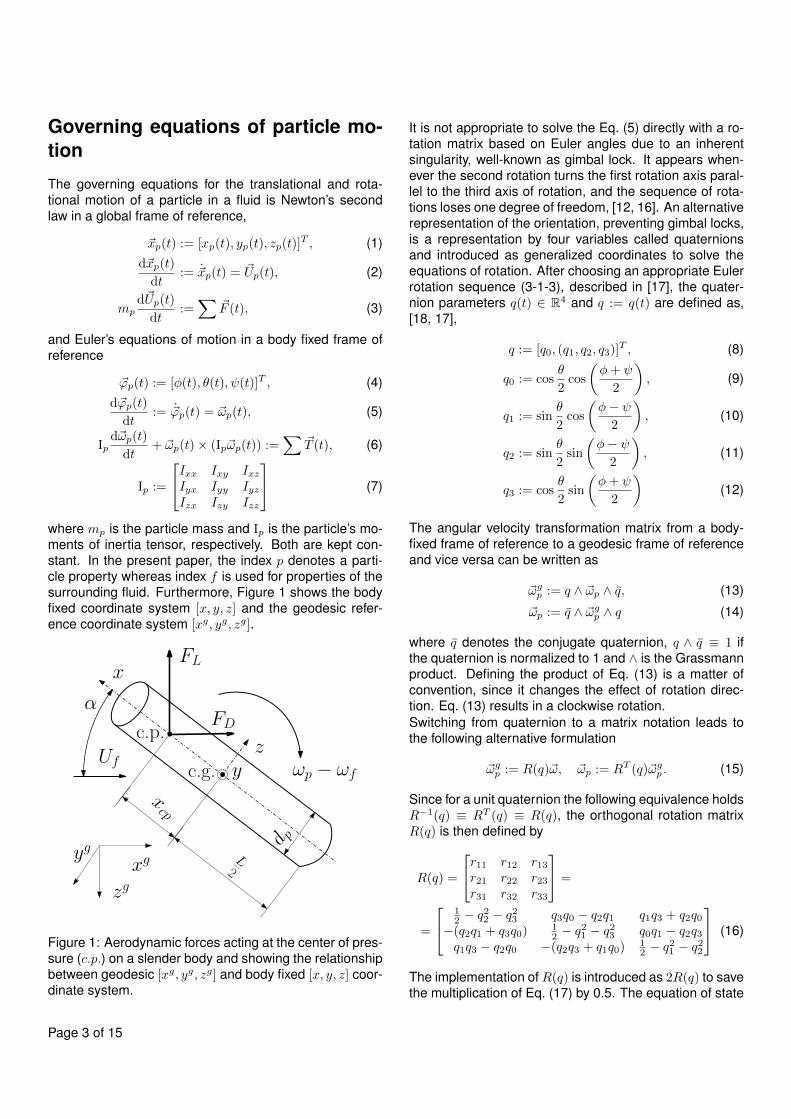
This effect is well seen in the contour plot of the Machnumber in Figure 17. At the front gap, the flow veloc-ity is approximately doubled from underneath the airfoilthrough the upper side. It is also obvious, that two recir-culation regions appear at the back of the slat and mainairfoil element with low flow velocities.

Page 11 of 15

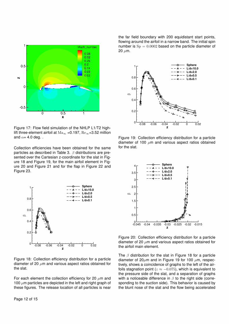
Figure 17: Flow field simulation of the NHLP L1/T2 high-lift three-element airfoil at Ma∞ =0.197, Re∞=3.52 millionand α= 4.0 deg. .

Collection efficiencies have been obtained for the sameparticles as described in Table 3. β distributions are pre-sented over the Cartesian z-coordinate for the slat in Fig-ure 18 and Figure 19, for the main airfoil element in Fig-ure 20 and Figure 21 and for the flap in Figure 22 andFigure 23.

z­0.08 ­0.06 ­0.04 ­0.02 0 0.02

0

0.2

0.4

0.6

0.8

1Sphere

L/d=10.0

L/d=2.0

L/d=0.5

L/d=0.1

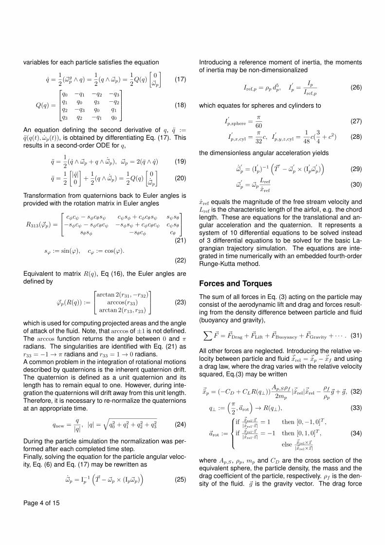
Figure 18: Collection efficiency distribution for a particlediameter of 20 µm and various aspect ratios obtained forthe slat.

For each element the collection efficiency for 20 µm and100 µm particles are depicted in the left and right graph ofthese figures. The release location of all particles is near

the far field boundary with 200 equidistant start points,flowing around the airfoil in a narrow band. The initial spinnumber is Sp = 0.0002 based on the particle diameter of20 µm.

z­0.08 ­0.06 ­0.04 ­0.02 0 0.02

0

0.2

0.4

0.6

0.8

1Sphere

L/d=10.0

L/d=2.0

L/d=0.5

L/d=0.1

Figure 19: Collection efficiency distribution for a particlediameter of 100 µm and various aspect ratios obtainedfor the slat.

z­0.045 ­0.04 ­0.035 ­0.03 ­0.025 ­0.02 ­0.015

0

0.5

1

1.5

2

2.5

3

3.5

4Sphere

L/d=10.0

L/d=2.0

L/d=0.5

L/d=0.1

Figure 20: Collection efficiency distribution for a particlediameter of 20 µm and various aspect ratios obtained forthe airfoil main element.

The β distribution for the slat in Figure 18 for a particlediameter of 20µm and in Figure 19 for 100 µm, respec-tively, shows a coincidence of graphs to the left of the air-foils stagnation point (z ≈ −0.075), which is equivalent tothe pressure side of the slat, and a separation of graphswith a noticeable difference in β to the right side (corre-sponding to the suction side). This behavior is caused bythe blunt nose of the slat and the flow being accelerated

Page 12 of 15

on the suction side. Surprisingly, no particles reached therecirculation region.

z­0.045 ­0.04 ­0.035 ­0.03 ­0.025 ­0.02 ­0.015

0

0.2

0.4

0.6

0.8

1Sphere

L/d=10.0

L/d=2.0

L/d=0.5

L/d=0.1

Figure 21: Collection efficiency distribution for a particlediameter of 100 µm and various aspect ratios obtainedfor the airfoil main element.

The graph in Figure 20 for particle diameters of 20 µmshows a β exceeding a value of 1 for the sphere, a cylin-der with L/dp = 2 and the disc with L/dp = 0.5. Thereason for this behavior is the small gap between slat andmain airfoil element. The stream tube formed by the parti-cles initially released is compressed while sliding throughthe gap between slat and main airfoil element, resulting ina smaller impingement area. Otherwise, β is different atthe stagnation point of the main airfoil element only. A bitmore challenging is the interpretation of the graph in Fig-ure 21 for the particle diameter of 100 µm. The C-shapeddistribution is caused by impingement on the whole bot-tom side of the main airfoil element. The upper part of thecurve until the reversal point is from the stagnation pointat the nose to the lowest z-coordinate of the main airfoil el-ement, which corresponds approximately to the mid-pointof the airfoil on the lower side. The graph shows a narrowspread in the β distribution, a reverted effect compared tothe slat. Because of the angle of attack at the slat andmain airfoil element, the exposed and shadow areas havereverted. The cylindrical particle with L/dp = 10 hits thebottom of the main airfoil element surface only until theminimum z-coordinate is reached.

z­0.12 ­0.1 ­0.08 ­0.06 ­0.04 ­0.02 00

0.2

0.4

0.6

0.8

1Sphere

L/d=10.0

L/d=2.0

L/d=0.5

L/d=0.1

Figure 22: Collection efficiency distribution for a particlediameter of 20 µm and various aspect ratios obtained forthe flap.

z­0.12 ­0.1 ­0.08 ­0.06 ­0.04 ­0.02 00

0.2

0.4

0.6

0.8

1Sphere

L/d=10.0

L/d=2.0

L/d=0.5

L/d=0.1

Figure 23: Collection efficiency distribution for a particlediameter of 100 µm and various aspect ratios obtainedfor the flap.

The particle impingement on the flap, Figure 22 and Fig-ure 23, is comparable to the main airfoil element since itis mainly impacted on the lower side. However, particlesreach the upper side of the airfoil in a narrow band fromthe β-peak to the right end of the curves, which is visi-ble in both figures. The maximum difference occurs in theregion of the β maximum and particularly the cylindricalparticle with L/dp = 10 has a distinctly larger βmax com-pared to all other particle types.Whenever it comes to industrial applications, the com-putational effort is often a measure for the applicability,results are given in Table 5. The simulation of spheres

Page 13 of 15

without rotation has been used as reference since it wasthe previous standard. The time ratio ξ = trot/tno-rot isthe time for computing rotating particles divided by thetime required for the non-rotating particles, each mea-sured for 200 trajectories. The standard implementationhas to solve six equations, three for the path and three forthe velocity in a three-dimensional context. Now, for therotation, seven additional equations need to be solved,four quaternion parameters and three for the particle an-gular velocity, which means that the number of equationsto be solved is more than doubled.

Table 5: Computational effort for the trajectory sim-ulation of the NHLP L1/T2 airfoil with the time factorξ = tno-rot/trot.

Particle-Shape L/dp tno-rot (s) trot (s) ξ

20 µm

Sphere 1 10.54 - 1Cylinder 10 - 45.05 4.3Cylinder 2 - 45.53 4.3Cylinder 0.5 - 47.39 4.5Cylinder 0.1 - 50.21 4.8

100 µm

Sphere 1 5.69 - 1Cylinder 10 - 18.35 3.2Cylinder 2 - 17.62 3.1Cylinder 0.5 - 19.49 3.4Cylinder 0.1 - 20.87 3.7

In summary, depending on the considered particle dimen-sions and flow conditions, an additional factor of three tofour needs to be expected in terms of computing time if theinfluence of rotation plays an important role and needs tobe considered.

Conclusion

A Lagrangian-type particle tracer based on the TAU Codehas been presented, taking into account rotation of reg-ular shaped particles. Validation of the implementationwas based on a comparison of analytical solutions and lit-erature based data and correlations for drag, forces andtorques. However, no validation was possible using thestandard way, e.g. by comparing trajectory paths or im-pingement distributions with experiments.The influence of considering particle rotation on the col-lection efficiency is strongly linked to the application. Itmay be negligible for a transport aircraft cruising at highaltitudes and transonic flow conditions with a moderatelyblunt nose. The situation changes significantly for airfoilsor wings generating a high circulation as it is often re-quired during take-off and landing at subsonic flow condi-

tions. Particularly, in flow regions exposed to strong flowaccelerations or decelerations as seen in the gaps be-tween a slat and the main airfoil element and the mainairfoil element and a flap or at the airfoil stagnation point.

References

[1] A. Haider, O. Levenspiel, Drag coefficient and ter-minal velocity of spherical and nonspherical parti-cles, Powder Technology 58 (1) (1989) 63–70. doi:10.1016/0032-5910(89)80008-7.

[2] G. H. Ganser, A rational approach to drag predic-tion of spherical and nonspherical particles, PowderTechnology 77 (2) (1993) 143–152. doi:10.1016/0032-5910(93)80051-B.

[3] S. Tran-Cong, M. Gay, E. E. Michaelides, Drag coef-ficients of irregularly shaped particles, Powder Tech-nology 139 (2004) 21–32. doi:10.1016/j.powtec.2003.10.002.

[4] G. B. Jeffery, The Motion of Ellipsoidal Particles Im-mersed in a Viscous Fluid, in: Proc. R. Soc. Lond.A, Vol. 102, 1922, pp. 161–179. doi:10.1098/rspa.1922.0078.

[5] R. G. Cox, The motion of long slender bodies in a vis-cous fluid: Part I General theory, J. Fluid Mech. 44 (4)(1970) 791–810. doi:10.1017/S002211207000215X.

[6] D. Qi, Lattice-Boltzmann simualtions of particles innon-zero-Reynolds-number flows, J. Fluid Mech. 385(1999) 41–62. doi:10.1017/S0022112099004401.

[7] H. Huang, X. Yang, M. Krafczyk, X.-Y. Lu, Rotation ofspheroidal particles in coutte flows, Journal of FluidMechanics 692 (2012) 369–394. doi:10.1017/jfm.2011.519.

[8] L. Rosendahl, Using a multi-parameter particleshape description to predict the motion of non-spherical particle shapes in swirling flow, AppliedMathematical Modelling 24 (1) (2000) 11–25. doi:10.1016/S0307-904X(99)00023-2.

[9] E. Loth, Lift of a Solid Spherical Particle Subject toVorticity and/or Spin, AIAA Journal 46 (2008) 801–809. doi:10.2514/1.29159.

[10] M. Mandø, L. Rosendahl, On the motion of non-spherical particles at high Reynolds number, PowderTechnology 202 (1-3) (2010) 1–13. doi:10.1016/j.powtec.2010.05.001.

[11] C. Kleinstreuer, Y. Feng, Computational Analysis ofNon-Spherical Particle Transport and Deposition in

Page 14 of 15

Shear Flow With Application to Lung Aerosol Dynam-ics - A Review, Journal of Biomenchanic Engineering135 (2013) 1–19. doi:10.1115/1.4023236.

[12] R. Zimmermann, Y. Gasteuil, M. Bourgoin, R. Volk,A. Pumir, J.-F. Pinton, Tracking the dynamics oftranslation and absolute orientation of a sphere ina turbulent flow, Review of Scientific Instruments82 (033906) (2011) 1–9. doi:10.1063/1.3554304.

[13] M. Widhalm, A. Ronzheimer, J. Meyer, LagrangianParticle Tracking on Large Unstructured Three-Dimensional Meshes, in: 46th AIAA Aerospace Sci-ences Meeting and Exhibit, AIAA 2008-472, Reno,NV, 2008.

[14] I. Langmuir, K. B. Blodgett, U. S. A. A. Forces, AMathematical Investigation of Water Droplet Trajec-tories, no. 5418 in Army Air Forces technical report,Army Air Forces Headquarters, Air Technical ServiceCommand, 1946.

[15] A. Hölzer, M. Sommerfeld, New simple correlationformula for the drag coefficient of non-spherical par-ticles, Powder Technology 184 (3) (2008) 361–365.doi:10.1016/j.powtec.2007.08.021.

[16] B. Kenwright, A beginners guide to dual-quaternion,in: V. Skala (Ed.), 20th WSCG International Confer-ence on Computer Graphics, Visualization and Com-puter Vision, Plzen, 2012.

[17] J. Diebel, Representing attitude: Euler angles, unitquaternions, and rotation vectors, University Lecture,Stanford University (2006).

[18] D. J. Evans, On the representation of orientationspace, Mol. Phys. 34 (2) (1977) 317–325. doi:10.1080/00268977700101751.

[19] A. Hölzer, M. Sommerfeld, Lattice boltzmann simula-tions to determine drag, lift and torque acting on non-spherical particles, Computers & Fluids 38 (2009)572–589. doi:10.1016/j.compfluid.2008.06.001.

[20] H. Wadell, The Coefficient of Resistance as aFunction of Reynolds Number for Solids of VariousShapes, Journal of the Franklin Institute 217 (4)(1934) 459–490. doi:10.1016/S0016-0032(34)90508-1.

[21] S. F. Hörner, Fluid-Dynamic Drag, published by theauthor, 1965.

[22] C. Yin, L. Rosendahl, S. Knudsen, H. Sørensen,Modelling the motion of cylindrical particles ina nonuniform flow, Chemical Engineering Sci-ence 58 (15) (2003) 3489–3498. doi:10.1016/S0009-2509(03)00214-8.

[23] F. M. White, Viscous fluid flow, 2nd Edition, McGraw-Hill, Inc., 1991.

[24] S. C. R. Dennis, D. B. Ingham, S. N. Singh, Thesteady flow of a viscous fluid due to a rotatingsphere, Quarterly Journal of Mechanics and AppliedMathematics 34 (3) (1981) 361–373.

[25] M. Zastawny, G. Mallouppas, F. Zhoa, B. vanWachem, Derivation of drag and lift force and torquecoefficients for non-spherical particles in flow, Inter-national Journal of Multiphase Flow 39 (2012) 227–239. doi:j.ijmultiphaseflow.2011.09.004.

[26] F. D. A. Grandin, J.-L. Brenguier, F. Hervy, H. Schal-ger, P. Villedieu, G. Zalamansky, HAIC (High AltitudeIce Crystals), American Institute of Aeronautics andAstronautics, 2013. doi:10.2514/6.2013-2674.

[27] M. Burns, A Selection of Experimental Test Cases forthe Validation of CFD Codes, Tech. rep., AGARD AR303, Vol. I, chapter 5 (1994).

[28] P. R. Spalart, S. R. Allmaras, A one-equation turbu-lence model for aerodynamic flows, AIAA Paper 92-0439, 1992.

Acknowledgement

The research leading to these results has received fund-ing from the European Union Seventh Framework Pro-gramme FP7/2007-2013 under grant agreement noACP2-GA-2012-314314 (HAIC - High Altitude Ice Crystals). Theauthor would like to thank Christian Bartels, Airbus GroupHamburg for his support and fruitful discussions duringthe detailed implementation of the features described inthis paper.

Page 15 of 15