Lagrangian Mixing Dynamics at the Cloudy–Clear Air Interface

BIPIN KUMAR

Max Planck Institute f€ur Meteorologie, Hamburg, Germany

JORG SCHUMACHER

Technische Universit€at Ilmenau, Ilmenau, Germany

RAYMOND A. SHAW

Department of Physics, Michigan Technological University, Houghton, Michigan

(Manuscript received 5 September 2013, in final form 30 January 2014)

ABSTRACT

The entrainment of clear air and its subsequent mixing with a filament of cloudy air, as occurs at theedge of a cloud, is studied in three-dimensional direct numerical simulations that combine the Euleriandescription of the turbulent velocity, temperature, and vapor fields with a Lagrangian cloud dropletensemble. Forced and decaying turbulence is considered, such as when the dynamics around the filamentis driven by larger-scale eddies or during the final period of the life cycle of a cloud. The microphysicalresponse depicted in nd2 hr3i space (where nd and r are droplet number density and radius, respectively)shows characteristics of both homogeneous and inhomogeneous mixing, depending on the Damk€ohlernumber. The transition from inhomogeneous to homogeneous mixing leads to an offset of the homog-eneous mixing curve to larger dilution fractions. The response of the system is governed by the smaller ofthe single droplet evaporation time scale and the bulk phase relaxation time scale. Variability within thend 2 hr3i space increases with decreasing sample volume, especially during the mixing transients. All ofthese factors have implications for the interpretation of measurements in clouds. The qualitative mixingbehavior changes for forced versus decaying turbulence, with the latter yielding remnant patches ofunmixed cloud and stronger fluctuations. Buoyancy due to droplet evaporation is observed to playa minor role in the mixing for the present configuration. Finally, the mixing process leads to the transientformation of a pronounced nearly exponential tail of the probability density function of the Lagrangiansupersaturation, and a similar tail emerges in the droplet size distribution under inhomogeneousconditions.

1. Introduction

The turbulent mixing of cloudy and clear air involvesa broad range of spatial and temporal scales, over whichwater vapor density and temperature fields are coupledto cloud droplet response through evaporation and theassociated enthalpy of vaporization. In this work, westudy the response of a population of cloud droplets toentrainment and mixing, including the active thermalfeedback. Upon the mixing of cloudy and clear air, and

assuming there is sufficient condensed water in the initialcloud, droplets will evaporate until the mixture becomessaturated. The final, uniquely defined thermodynamicstate, however, can be achieved through very differentmicrophysical manifestations. For example, the final,diluted liquid water content (LWC) could be reachedin one extreme due to all droplets evaporating by thesame amount or in the other extreme due to a subset ofdroplets evaporating completely, leaving the remainingdroplets unchanged. These extremes were first recognizedby Latham and Reed (1977) and Baker et al. (1980, 1984),who described them as homogeneous and inhomoge-neous mixing, respectively. The limits can be convenient-ly expressed through the Damk€ohler number, definedas the ratio of a fluid time scale to a characteristic

Corresponding author address: Bipin Kumar, Max Planck-Institut f€ur Meteorologie, Bundesstrasse 53, D-20146 Hamburg,Germany.E-mail: bipin.kumar@mpimet.mpg.de

2564 JOURNAL OF THE ATMOSPHER IC SC IENCES VOLUME 71

DOI: 10.1175/JAS-D-13-0294.1

! 2014 American Meteorological Society

thermodynamic time scale associated with the evap-oration process:

Da5tfluidtphase

, (1)

with homogeneous and inhomogeneous mixing corre-sponding to the limits Da! 1 and Da" 1, respectively(Lehmann et al. 2009; Andrejczuk et al. 2009). Homo-geneous mixing occurs when the evaporation of cloudwater droplets is slow compared to the mixing andtherefore takes place in a well-mixed, or in other words,homogenized environment. Inhomogeneous mixing oc-curs when the evaporation proceeds much faster thanthe turbulence evolves, with the result that droplets nearthe clear air–cloud interface experience evaporationwhile others do not. Both processes can coexist in aturbulent cloud because of the broad spectrum of fluidtime scales that are present, with inhomogeneousmixingdominating at large scales and homogeneous mixingoccurring at fine scales (Lehmann et al. 2009).The characteristic time scale associated with the re-

sponse of the water vapor density and temperature fieldsas a result of droplet growth or evaporation is the phaserelaxation time tphase, which is inversely proportional tothe droplet number density and the mean droplet radius(e.g., Kostinski 2009; Kumar et al. 2013). For smalldroplets or strong dilution by dry air, complete evapo-ration can occur, suggesting that the appropriate mi-crophysical response time should be the single dropletevaporation time scale tevap (cf. Andrejczuk et al. 2006).It was argued by Lehmann et al. (2009) that the smallerof the two time scales tphase and tevap is the appropriateone for specifying Da and therefore the relative homo-geneity of themixing process, and that suggestion will befurther addressed here.The mixing problem has been approached in many

recent studies from the point of view of a mixing dia-gram showing the microphysical response in terms ofcloud droplet mean volume radius hr3i versus numberdensity nd. This nd 2 hr3i space, introduced by Jensenet al. (1985), allows a reduction in liquid water content,W} ndhr3i, to be interpreted as the relative reductions incloud droplet number density (through both dilutionand total droplet evaporation) and mean droplet di-ameter. Andrejczuk et al. (2006) were the first to showa ‘‘trajectory’’ within a mixing diagram. Note that thesetrajectories are for averages taken over the entire volumeand are for a ‘‘bulk’’ cloud treatment. General consis-tency with scaling laws was found. For example, largerdroplets gave a more homogeneous mixing signature. Ina subsequent paper, Andrejczuk et al. (2009) studiedthe ratio of time scales in their numerical simulation, in

particular the ratio of the turbulence time scale to thedroplet evaporation time scale, thereby supporting quan-tification via the Damk€ohler number [cf. Eq. (1)]. Ina thorough study of measured cloud properties in themixing diagram, Burnet and Brenguier (2007) showed adistinct predominance for inhomogeneous mixing. Theypoint out that the difficulty in observing homogeneousmixing in clouds may in some cases be a sampling arti-fact resulting from spatial averaging. Gerber et al. (2008)also detected in their measurements signatures that in-dicate strong inhomogeneousmixing, but they suggest thepossibility that the data could be interpreted as resultingfrom homogeneous mixing with a small contrast betweencloud and environment. The possibility of mixing withalready humid air is consistent with the finding of Heusand Jonker (2008), who showed with large-eddy simu-lations that cumulus clouds are surrounded by subsidingshells in which fluid motion is mostly downward. Thus,the mixing takes place rather locally with diluted cloudyair in the vicinity of the interface rather than with alarge-scale environment. These numerical results implyalready that homogeneous and inhomogeneous mixingcan coexist and are sometimes difficult to disentangle.Finally, Lehmann et al. (2009) gave theoretical argu-ments and field data in support of the concept that asingle Damk€ohler number is not sufficient to explain themixing. Based on the cascade concept in turbulence,they also suggest a length scale at which the systemtransforms from dominantly homogeneous to inhomo-geneous mixing.Kumar et al. (2012) studied extremes of mixing, not

via range of scales, but by enhanced or suppresseddroplet response within an Euler–Lagrangian model.The studies showed that a Da similarity does exist withinthe range of idealized conditions studied. In otherwords, they observed that different turbulent and mi-crophysical initial conditions having the same Da willtend to the same final microphysical state when themixing process is completed. Kumar et al. (2013) in-vestigated the phase relaxation process during a mixingevent under a variety of realistic microphysical condi-tions for a cumulus cloud. In this Lagrangian view of themixing process, a range of Da was investigated, and itwas shown that the relevant microphysical time scale isthe ‘‘diluted’’ phase relaxation time (i.e., calculated withthe number density based on the whole volume). In bothof these studies, however, the simulations did not in-clude the temperature field and therefore the interactionbetween latent heat and dynamic coupling throughchanges in buoyancy.Besides numerical studies and measurements, a third

effort consists of the development of parameterizedmodels describing the essentials of the simultaneous

JULY 2014 KUMAR ET AL . 2565

mixing at multiple scales. Krueger et al. (1997) and Suet al. (1998) pioneered the extension of the linear eddymodel to the entrainment problem, thereby enabling therepresentation of cloud mixing and microphysical re-sponse on multiple length scales without a direct simu-lation. Such models can be potentially incorporated intocloud physics parameterizations in larger-scale modelsthat do not resolve processes below a few kilometers.In a different approach based on the simulations ofAndrejczuk et al. (2006), Grabowski (2007) suggesteda simple, subgrid parameterization of cloud droplet re-sponses to bulk mixing based on increasing fila-mentation of the turbulent eddies in a steady cascadeprocess. Lu et al. (2011) explored the possibility ofrepresenting subgrid mixing effects on microphysics viaa dimensionless parameter, the scale number, to char-acterize the dynamics of different entrainment-mixingprocesses. The scale number relates the transition-scaleconcept of Lehmann et al. (2009) to the Kolmogorovlength, the mean dissipation scale of the turbulence. Luet al. (2013) have coupled measurements and modelingstudies using the linear eddy approach to explore thedegree of homogeneous mixing and its dependence ontransition scales.Prior computational investigations of the mixing

process, such as those by Jensen and Baker (1989),Andrejczuk et al. (2004, 2006), Malinowski et al. (2008),and de Lozar and Mellado (2014), have considered theproblem primarily from the continuum microphysicsperspective. De Lozar and Mellado (2014) includedsome more detailed processes such as droplet sedi-mentation and particle inertia in their bulk formulation.Here, we explore what additional insight can be gainedby explicitly treating the Lagrangian nature of the dis-crete droplet field, including droplet inertia and gravi-tational sedimentation. The coupling of Lagrangiandroplets to the Eulerian vapor density and temperaturefields is similar to the approaches of Vaillancourt et al.(2001, 2002) and Lanotte et al. (2009); in those studiesthe emphasis was on the evolution of the supersatura-tion field and the droplet population during steadygrowth, instead of the microphysical response to a tran-sient mixing event considered here.In this work, we consider an idealized cloud slab that

mixes with a dry environment in a small subvolume atthe edge of a cloud. The simple geometry allows fora clearly defined initial scale for the mixing. The initialcloud and environment values are purposely set torather extreme values, and the motivation for this isexplained here. First, the environment is essentiallycompletely dry so that a strong signature of homoge-neous mixing can be observed. Observational studiesoften show rather inhomogeneous signatures, and this

can be a result of mixing with very humid air even underhomogeneous conditions (e.g., Gerber et al. 2008).Second, the initial cloud is taken to have a range ofliquid water content so that cases with partial and withcomplete evaporation of droplets can be studied. Toachieve partial evaporation, very large initial liquidwater contents are set in themost extreme case. The goalis to understand the microphysical response to mixing ina wide range of parameter space, as opposed to simu-lating only ‘‘typical’’ cloud conditions.Wewill study twodifferent flow scenarios: decaying convective (D) andstationary convective (S) runs. The decaying convectiveruns study the mixing in a decaying turbulent case withfeedback by buoyancy. In the stationary convectiveruns, the mixing proceeds in a statistically stationaryflow sustained by an additional, steady driving force thatmimics the impact of larger-scale eddies on the dy-namics in the subvolume.Several consequences of a finescale study, as is

conducted here (approximately 0.1m3 are simulated),should be mentioned in order to place the work ina proper context. Because the subvolume in the presentsystem is rather small, diffusivities of the scalar fieldsare close to the kinematic viscosity magnitude, andtherefore advection and diffusion time scales do notdiffer by many orders of magnitude. Thus, the mixingprocess always incorporates both diffusion and stirring(or advection). Both processes cannot be separated fromeach other for the given parameters, as has been dis-cussed by Broadwell and Breidenthal (1982), Sreenivasanet al. (1989), and Malinowski and Zawadzki (1993). Thescale of this study also does not lend itself to definingthe simulated mixing process as entrainment versusdetrainment; in part because at finescales it is not ob-vious that a mean cloud surface can be defined, as isrequired for a formal distinction between the twoprocesses (de Rooy et al. 2013). The focus of the studyis on the microphysical response to mixing, regardlessof whether it is occurring in entrainment or detrainmentregions. Finally, a consequence of the relatively smallvolume, which can be simulated with existing compu-tational resources, is that the limit of extremely in-homogeneous mixing (Da " 1) is not investigated inthis work.The outline of the manuscript is as follows: The next

section describes the Euler–Lagrangian model andthe setting of the simulations. Section 3 starts witha brief discussion of the dynamics in both flow set-tings, followed by a detailed analysis of the mixingdiagrams. Furthermore, we compare Lagrangian dis-tributions of the droplet size and supersaturation atdroplet positions. We conclude with a summary andan outlook.

2566 JOURNAL OF THE ATMOSPHER IC SC IENCES VOLUME 71

2. Eulerian–Lagrangian Boussinesq modelof mixing

a. Model equations, parameters, and numericalmethod

The buoyancy B is a function of the temperature T,the vapor mixing ratio qy, and the liquid water mixingratio ql. The latter two quantities are defined as qy(x, t)5ry/rd and ql(x, t)5 rl/rd, where ry, rl, and rd are themassdensities of vapor, liquid water, and dry air, respectively.The Eulerian equations for the turbulent fields, namely,the velocity field u, the temperature field, and the vapormixing ratio field, are given by

$ # u5 0, (2)

›tu1 (u # $)u521

r0$p1 n=2u1Bez1 fLS , (3)

›tT1u # $T5 k=2T1L

cpCd , (4)

›tqy 1 u # $qy 5D=2qy 2Cd . (5)

The reference density r0 is the dry air density. Thebuoyancy term in the momentum equation is defined as

B(x, t)5 g

!T2T0

T0

1 ~!(qy 2 qy0)2 ql

", (6)

where ~!5Ry/Rd 2 1’ 0:608. Here, Ry is the vapor gasconstant, and Rd is the dry air gas constant. The addi-tional term fLS keeps the flow in a statistically stationarystate during the mixing process. It is used to model thedriving of the entrainment process resulting from largerscales (LS) that go beyond the volume size consideredhere. The term is implemented in the Fourier space inthe applied pseudospectral method and is given by (seealso Kumar et al. 2013)

fLS(k, t)5 !inu(k, t)

!kf2K

ju(kf , t)j2dk,kf

, (7)

with the Kronecker delta

dk,kf5 1 if k5 kf , dk,k

f5 0 otherwise, (8)

and the wavevector subset K that contains a few wave-vectors. Here, thesewavevectors are given by kf5 (2p/Lx,2p/Ly, 4p/Lz) plus all permutations with respect to com-ponents and signs. Physically, we inject a fixed amount ofturbulent kinetic energy per time unit into our flow suchthat, in a statistically stationary regime, the parameter !in

would equal the mean kinetic energy dissipation rate inthe flow when the buoyancy feedback would be absent(see also section 3a).We will denote runs with fLS 5 0 as decaying con-

vective runs and fLS 6¼ 0 as stationary convective runs.Furthermore, Cd is the condensation rate, n is the ki-nematic viscosity of air,D is the vapor mass diffusivity, kis the thermal diffusivity, cp is the specific heat at con-stant pressure, and L is the latent heat. The problem isstudied in a cube (i.e., Lx 5 Ly 5 Lz) with periodicboundary conditions in all three spatial directions. It isspanned by an equidistant mesh with uniform sizea equal to the Kolmogorov length hK. Further parame-ters of the initial setup are listed in Table 1. The equa-tions are solved by a standard pseudospectral methodthat uses three-dimensional fast Fourier transformations(Ferziger and Peri"c 2001; Spyksma et al. 2006). Timestepping for the Eulerian and Lagrangian parts is doneby a second-order predictor–corrector scheme.The liquid water component is modeled as a La-

grangian ensemble of N pointlike droplets. From thisensemble, the liquid water mixing ratio and the con-densation rate are obtained. The droplets are de-scribed by

dX

dt5V(X, t) , (9)

dV

dt5

1

tp[u(X, t)2V(X, t)]1 g , (10)

r(X, t)dr(X, t)

dt5KS(X, t) . (11)

Here, X is the droplet position, V is its velocity, and r isthe radius. We describe cloud water droplets as inertialpoint particles with a finite particle response time tp 52rlr

2/(9r0n) that can grow and shrink by diffusion ofvapor to their surface. The vector g5 (0, 0,2g) includes

TABLE 1. Parameters of the initial turbulence conditions for allparameter runs. The root-mean-square velocity is calculated byurms 5 hu2i i

1/2, the Kolmogorov length is calculated by hK 5 n3/4/h«i1/4, and the Kolmogorov time is calculated by th 5 (n/h«i)1/2.

Quantity Symbol Value

Grid points N 512Box length Lx 51.2 cmGrid size a 1mmKinematic viscosity of air n 1.5 3 1025m2 s21

Mean energy dissipation rate h«i 33.75 cm2 s23

Kolmogorov length hK 1mmKolmogorov time th 0.066 sRoot-mean-square velocity urms 12.5 cm s21

Large-scale turnover time TL 4.1 s

JULY 2014 KUMAR ET AL . 2567

the gravitational acceleration g. The constant K in Eq.(11) is a function of temperature and pressure and in-corporates the self-limiting effects of latent heat ex-change (e.g., Rogers and Yau 1989). This diffusionalgrowth is controlled by the supersaturation, given byS(X, t) 5 qy(X, t)/qy,s(T) 2 1. The saturation vapormixing ratio qy,s(T) has to be determined from thetemperature via the Clausius–Clapeyron equation. Fora more detailed derivation of Eq. (11) and its im-plementation in the simulation, we refer the reader toKumar et al. (2013). To close the set of equations, wedetermine the condensation rate field Cd(x, t) followingVaillancourt et al. (2001, 2002) by

Cd(x, t)54prlK

r0a3 !

4

b51S(Xb, t)r(Xb, t) . (12)

Here, ma is the mass of air per grid cell, and the sumcollects the droplets inside each of the grid cells of size a3

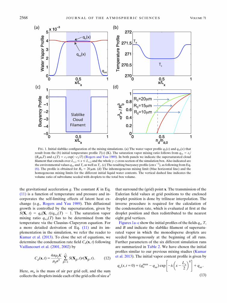
that surround the (grid) point x. The transmission of theEulerian field values at grid positions to the encloseddroplet position is done by trilinear interpolation. Theinverse procedure is required for the calculation ofthe condensation rate, which is evaluated at first at thedroplet position and then redistributed to the nearesteight grid vertices.Figures 1a–c show the initial profiles of the fields qy,T,

and B and indicate the slablike filament of supersatu-rated vapor in which the monodisperse droplets areseeded homogeneously at the beginning of all runs.Further parameters of the six different simulation runsare summarized in Table 2. We have chosen the initialprofiles similar to our previous mixing studies (Kumaret al. 2013). The initial vapor content profile is given by

qy(x, t5 0)5 (qmaxy 2 qye) exp

"2l

#x2

Lx

2

$8#1 qye .

(13)

FIG. 1. Initial slablike configuration of the mixing simulations. (a) The water vapor profile qy(x) and qys(x) thatresult from the (b) initial temperature profile T(x) (K). The saturation vapor mixing ratio follows from qys 5 es/(Ryr0T) and es(T) 5 c1 exp(2c2/T) (Rogers and Yau 1989). In both panels we indicate the supersaturated cloudfilament that extends over Lx,1 # x# Lx,2 and the whole y–z cross section of the simulation box. Also indicated arethe environmental values qye and Te as well as Tc. (c) The resulting buoyancy profile (cm s22), as following fromEq.(6). The profile is obtained for R0 5 20mm. (d) The inhomogeneous mixing limit (blue horizontal line) and thehomogeneous mixing limits for the different initial liquid water contents. The vertical dashed line indicates thevolume ratio of subvolume seeded with droplets to the total box volume.

2568 JOURNAL OF THE ATMOSPHER IC SC IENCES VOLUME 71

Here, qmaxy is the maximum amplitude of qy, which ex-

ceeds qys by 2%, and l5 1.03 10210 cm21 is a constant.The initial temperature profile is chosen such that bothdo not contribute jointly to the initial buoyancy, thatis, T(x, t5 0)5T0 2 ~!T0[qy(x, t5 0)2qy0], as derivedfrom Eq. (6). The reference values are given by thevolume averagesT05 hT(t5 0)iV and qy05 hqy(t5 0)iV.Other initial configurations are possible. Ourmotivationis to use an initial condition with a well-defined inter-face that is still a smooth function and avoids the Gibbsphenomenon, that is, numerical overshoots at sharpinterfaces.All runs start with the same turbulent flow field that

has been generated in a pure fluid simulation of statis-tically stationary box turbulence ahead of the entrain-ment runs. The focus of the study is on the entrainmentprocess, and therefore we neglect droplet collisions. Thisis physically reasonable given the short mixing timessimulated relative to typical droplet collision time scales.

b. Homogeneous and inhomogeneous mixing limits

The central dimensionless parameter that quantifiesthe mixing of clear and cloudy air is the Damk€ohlernumber defined in Eq. (1). The fluid time scales covera whole spectrum of values and can vary from the large-eddy turnover time TL 5 Lx/urms to the Kolmogorovtime scale th 5 (n/h«i)1/2. The evaporation process ischaracterized by the phase relaxation time, given ap-proximately by

tphase 51

4pDndR0

, (14)

where nd is the number density of the droplets, and D isthe vapor diffusion constant that contains the self-limiting effects of latent heat release as described inKumar et al. (2012). The inhomogeneous limit stands for

a very rapid evaporation compared to the evolution timeof the fluid. Droplets at the cloud interface will evapo-rate immediately, while droplets in the center of thecloud remain unaffected by the mixing of the clear airinto the cloudy filament. As a consequence, the numberdensity decreases, while the mean cubic radius hr3iremains essentially unchanged. In a mixing diagramshowing hr3i/R3

0 plotted against nd/nd,0, such a process isgiven by a horizontal line (Jensen et al. 1985; Burnet andBrenguier 2007; Gerber et al. 2008; Lehmann et al.2009), as shown in Fig. 1d. A second time scale related tothe droplet response is the evaporation time given by

tevap52r2

2KS, (15)

which is a direct consequence of Eq. (11) in the case ofa constant supersaturation.The homogeneous mixing limit assumes a slow micro-

physical response time scale such that the whole cloudwater droplet ensemble evolves in a well-mixed environ-ment. The corresponding mixing lines for the three dif-ferent initial radii and the parameters of the initialconfiguration are also indicated in Fig. 1d. The calculationof these lines is performed as follows: it is assumed thatprecipitation is absent and that the total water content andthe liquid water potential temperature, ul 5 T2 (L/cp)ql,are state variables that describe the air parcels. Becausethey are conserved duringmixing the following two simplerelations hold (e.g., Gerber et al. 2008):

ql 1 qys(T)5 x[qlc1 qysc(Tc)]1 (12 x)qye , (16)

T2L

cpql 5x

Tc 2

L

cpqlc

!1 (12 x)Te , (17)

with (Rogers and Yau 1989)

TABLE 2. Parameters of the six DNS runs. We list the initial droplet radius R0, initial liquid water contentW, the number density in theundiluted initial slablike cloud filament, the phase relaxation time tphase, the single droplet evaporation time given by tevap 52R2

0/(2KS0)[cf. Eq. (15)], the Damk€ohler numbers based on the Kolmogorov and large-eddy scales, and the Damk€ohler numbers calculated with theevaporation time scale (rather than the usual phase relaxation time scale). The superscript (0) indicates that the calculations are based onvalues at the beginning of the simulation (t5 0). The large-eddy time for all runs isTL5 4.1 s; theKolmogorov time is th5 0.066 s (see alsoTable 1). Two scenarios apply here: the purely convective feedback (D1–D3) to the velocity field via the buoyancy term B as given inEq. (6) or the buoyancy feedback that is combinedwith an additional volume driving fLS beside the buoyancy feedback (S1–S3). The lattermimics the motion of larger turbulent eddies that feed energy into the present subsystem (Schumacher et al. 2007). The slablike cloudyfilament is filled with 8.8 million droplets.

Case R0 (mm) W (g cm23) n(0)d (cm23) t(0)phase (s) t(0)evap (s) Da(0)h Da(0)L Da(0)h,evap Da(0)L,evap

S1 10 0.37 153 4.12 0.93 0.016 1.0 0.07 4.4S2 15 1.24 153 2.75 2.10 0.024 1.5 0.03 2.0S3 20 2.95 153 2.06 3.73 0.032 2.0 0.02 1.1D1 10 0.37 153 4.12 0.93 0.016 1.0 0.07 4.4D2 15 1.24 153 2.75 2.10 0.024 1.5 0.03 2.0D3 20 2.95 153 2.06 3.73 0.032 2.0 0.02 1.1

JULY 2014 KUMAR ET AL . 2569

qys(T)’c1 exp(2c2/T)

Ryr0T, (18)

with c1 5 2.53 3 108 kPa and c2 5 5420K. Here, x isdefined as the mixture fraction; indices c and e stand forcloud and environment, respectively. This nonlinearsystem of Eqs. (16)–(18) has to be solved by a root-finding algorithm and results in ql(x) and T(x) valuescorresponding to a given x. The quantity hr3i is obtainedvia ql5W/r0 andW5 4prlnd,0xhr3i. If it is assumed thatx 5 nd/nd,0, that is, all droplets respond equally and nosubset of droplets is allowed to evaporate completely,then this yields the homogeneous mixing curves in themixing diagram. The homogeneous mixing processstarts from point (1, 1) in the upper right andmoves fromone equilibrium state to another along the mixing lines.Different lines for the homogeneous limit correspond todifferent initial liquid water content W.

3. Simulation results

a. Turbulence in decaying and stationary convectiveregimes

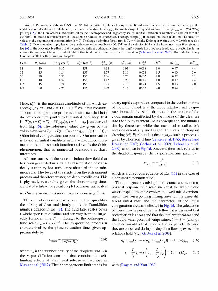
As already discussed in section 2, all simulations startwith a statistically stationary fluid turbulence state cor-responding to a Taylor microscale Reynolds number ofRl ’ 90. We either continue to sustain the driving fLS,and thus sustain statistical stationarity of the flow fieldduring the mixing event, which is done in the stationaryconvective regime for runs S1–S3, or we switch off theadditional driving, as done in the decaying convectiveruns D1–D3. In both cases, the feedback from thebuoyancy term Bez is present but turns out to be small.This is likely a result of the relatively low temperatureconsidered in this study. The dynamical evolution isclose to freely decaying turbulence for cases D1–D3.Note that we do not sustain a mean temperature gradi-ent with respect to z, which would cause a strongbuoyancy driving additionally amplified by the periodicboundary conditions (this regime is known as the ho-mogeneous Rayleigh–B"enard convection regime; e.g.,Calzavarini et al. 2006).Figure 2 (top) displays the temporal evolution of the

turbulent kinetic energy (TKE). As expected, we ob-serve that the TKE in runs S1–S3 remains on average atthe initial value while it decays within a few seconds forruns D1–D3. In the steady convective case,

h«(t)iV5 huzB(t)iV 1 hu # fLS(t)iV ’ hu # fLS(t)iV0h«iV,t ’ hu # fLS(t)iV,t . (19)

Buoyancy, as the lone driving force in the decay-ing convective cases, causes a transient growth, but

FIG. 2. (top) TKE (cm2 s22) vs time (s) for all six runs as indicatedin Table 2 (see legends). (middle) Variance of the vapor mixingratio fluctuations vs time (s). (bottom) Variance of temperaturefluctuations (K2) vs time (s).

2570 JOURNAL OF THE ATMOSPHER IC SC IENCES VOLUME 71

eventually the TKE and temperature fluctuations con-tinue to decay. The intermediate maximum is due tobuoyancy forcing, which acts as an amplifier when itsown amplitude is still large enough. When comparingu2i (x, t0) with u2z(x, t0), we observed that both quantitiesevolve in similar filaments for the period of the transientgrowth, that is, for a period that lasts for a few secondsstarting after 4–5 s. We interpret this finding as a clearindication that the initial buoyancy profile (as seen inFig. 1c) amplifies vertical velocity fluctuations primarily.Since the whole system decays in the meantime, theintermediate peak in the fluctuations can be interpretedby the coupling of vertical velocity and buoyancy for theperiod at which temperature differences are still largeenough. In turn, the transiently amplified vertical ve-locity fluctuations enhance the temperature fluctuationsfor this short period, which is displayed in Fig. 1c.The amplitude of the transient growth increases with

the amount of liquid water that is contained in the initialcloud slab. The middle panel of Fig. 2 displays thetemporal evolution of the variance of the vapor mixingratio fluctuations. The fluctuations are defined as

q0y(x, t)5 qy(x, t)2 hqy(t)iV , (20)

where we take the time-dependent volume mean corre-spondingly. The presence of the additional large-scaledriving enhances the decay. We also observe that dif-ferences among the three runs in each of the two seriesremain small, implying that the feedback from thecondensation rate source term in Eq. (5) remains verysmall. However, this difference is bigger in the stationarycase than in the decaying case. The bottom panel of Fig. 2displays the variance of the temperature field fluctua-tions, which have been calculated in the same way asthose of the vapor mixing ratio [cf. Eq. (20)]. The tran-sient growth depends now clearly on the flow regime andthe initial amount of liquid water in the slab. With in-creasing initial radius R0, as indicated in the legend, thetransient growth increases in amplitude and time, a man-ifestation of the enhanced contribution from the sourceterm in Eq. (4). The additional bulk forcing suppressesthis effect significantly as can be seen when comparingboth series. To summarize, the large-scale forcing fLSbrings the whole system close to the passive mixing casethat has been studied by Kumar et al. (2012, 2013).In the runs with additional driving, the mixing is

completed when the phase relaxation time is reached(see Table 2). The turbulence volume is uniformlymixed and turbulence remains in the statistically sta-tionary regime. In the decaying case, the system remainsin a transient that ends when the turbulence is com-pletely faded away.

b. Mixing diagrams

For the rest of the paper we focus on the microphys-ical response during the mixing process. To analyze theevolution in the mixing diagrams, we divide the initialslab into subdomains as displayed in Fig. 3. The dropletsseeded in the four subdomains are colored differentlyaccording to their initial locations, as shown in the toppanel. The bottom panel visualizes the initial distortionof the cloud slab, with some droplets entering regions ofenvironmental air and other droplets simply mixingwithin the cloud filament. The Lagrangian treatment ofindividual cloud droplets allows not only the bulk mi-crophysical properties of the cloud to be investigated,but the evolution of the full droplet size distribution.This includes, for example, the possibility of strong oreven complete evaporation of individual droplets thatexperience sudden exposure to dry environmental con-ditions during the early mixing transients.Mixing diagrams allow the microphysical response to

mixing to be viewed; that is, to what extent is a givenreduction in liquid water content W } ndhr3i due toa reduction in nd versus hr3i? The inhomogeneous andhomogeneous mixing lines plotted in the mixing dia-gram correspond to equilibrium, thermodynamic con-ditions under the two extremes for mixing. To whatextent the actual cloud microphysical conditions corre-spond to equilibrium states is not obvious, however,because until the mixing is complete the system can beconsidered to be transient. We follow Andrejczuk et al.(2009) therefore and plot microphysical trajectorieswithin the mixing diagram, so that the instantaneoustemporal evolution of microphysical properties can bevisualized. To define the droplet number density andmean radius, it is necessary to define a sample volume.We begin by dividing the volume into 16 equally sizedsubslabs that occupy the full width of the initial cloudfilament and are arranged 4 3 4 in the y and z di-mensions (as in Fig. 3, except each colored region thereis further divided into four subvolumes). Microphysicaltrajectories for runs S3 and D3, that is, for initial dropletradii of 20mm, are shown in the top panels of Fig. 4, andtrajectories for runs S2 and D2, that is, for initial dropletradii of 15mm, are shown in the bottom panels. A firstobservation is that the trajectories at least roughly tendto follow the homogeneousmixing line as opposed to theinhomogeneous mixing limit. In fact, while the in-dividual trajectories may deviate during the transientbehavior, the final points are quite close to the homo-geneous mixing curve. This builds confidence in thenotion that the Damk€ohler number, as defined here,indeed captures the essential behavior of the system. Assummarized in Table 2, Dah ! 1 in all cases, so the

JULY 2014 KUMAR ET AL . 2571

dissipation-scale mixing is expected to be strongly in thehomogeneous limit. Even for the large eddies, DaL ; 1,and so the largest simulated scales are only expected tobe in the transition range between homogeneous andinhomogeneous mixing. Indeed, a hint of this initiallyinhomogeneous behavior can be seen in the early tran-sient response, in which the trajectories can be observedto initially follow the horizontal mixing line (see espe-cially the bottom-left panel). Ultimately, a steady state isreached, and because the initial droplet radii are suffi-ciently large and the turbulent mixing is sufficientlyrapid, few droplets are able to completely evaporate andthe mean properties of the mixed-cloud approach thehomogeneous limit. As would be expected, the trajec-tories from the runs with smaller initial radius progressfarther down the homogeneous mixing lines comparedto those with larger initial radius: a straightforward re-sult of conservation of water mass, given the identicalenvironmental conditions in the two cases.Several differences are immediately evident when

comparing the stationary forced results (Fig. 4, left) andthe decaying results (Fig. 4, right). First, the variabilitybetween microphysical trajectories is significantly largerfor the decaying compared to the stationary turbulenceruns. Second, the endpoints of the trajectories of D3 andD2 do not reach as closely to the homogeneous mixingline, compared to S3 and S2. These observations can beinterpreted to result directly from the strongly sup-pressed fluctuations in vapor and temperature fields (seemiddle and bottom panels of Fig. 2) in the stationaryforced turbulence relative to the decaying turbulence.Qualitatively, the decaying turbulence dies out beforethe mixture has become thoroughly homogenized, al-lowing random fluctuations in temperature, vapor con-centration, and droplet number density to persist andtherefore for the resulting droplet radius fluctuations tobecome more pronounced. The scatter in the trajectoryendpoints is especially noticeable in run D2, with nd/nd,0ranging from approximately 0.4 to 0.6 even in the final,mixed state. It is also intriguing that in the top-rightpanel, corresponding to run D3, several subvolumesachieve nd/nd,0 . 1 during the initial mixing. In fact, injust a very short time, the trajectories span nd/nd,0 of 0.4–1.1 in that case, eventually homogenizing to a range ofDnd/nd,0 ’ 0.1.To investigate the possible influence of the sampling

geometry on the results, we vary the subslab size andshow the resulting trajectories in Fig. 5. For this com-parison, only results for the decaying turbulence D1 areshown. Here, there is complete evaporation of thecloud whenmixing is complete, but the trajectories showinteresting differences. In the case with fewer, largersubvolumes (4 vs 16), there is considerably less variability.

FIG. 3. Illustration of the Lagrangian mixing of the cloud waterdroplets. (top) Out of the 8.8 million droplets, we select 20 000droplets and color them differently based on their initial position inthe cloud filament. (bottom) The mixing and entrainment hasprogressed to 1.25 s or 0.3TL. This subdivision of the cloud filamentwill be also used later in the text when we discuss the mixing pro-cess in detail.

2572 JOURNAL OF THE ATMOSPHER IC SC IENCES VOLUME 71

This is not a surprise, since these coarser subvolumes arerather close to the large-eddy scale, whereas the smallersubvolumes lie in the inertial subrange. It should benoted that the very slight increases beyond hr3i/R3

0 5 1are a result of the small water vapor supersaturation inthe initial profile of qy (cf. Fig. 1).Especially interesting in the D1 run is the appearance

of what can be termed an inhomogeneous offset: thecurves appear quite similar to the shape of the homo-geneousmixing curve but are shifted to smaller values ofnd/nd,0. This can be interpreted as resulting from therelative magnitude of tphase and the single-droplet tevap.Case D1 with R0 5 10mm is the only scenario in whichtevap is significantly less than tphase. Lehmann et al.(2009) showed that the relevant microphysical timescale describing the response to turbulent mixing isthe smaller of tphase and tevap. That is because tphaseis calculated by assuming constant R, whereas tevap is

calculated by assuming constant S, neither strictly correct,but the smaller of two time scales indicating which as-sumption is more accurate. Defining a Damk€ohler num-ber based on tevap results in DaL,evap 5 4.4 for cases S1and D1, significantly greater than unity and thereforefavoring inhomogeneous mixing at the largest scales inthe inertial subrange. This can be quantified via thetransition length scale, defined as the length within theinertial subrange at which Da 5 1, that is,l*5 (t3evaph«i)

1/2. For case S1 and D1, we obtain l* 55 cm, which is a factor of 10 smaller than the large-eddyscale Lx and a factor of 50 greater than the Kolmogorovlength scale hK (see Table 1). The trajectories shown inFig. 5 therefore can be taken as direct demonstration ofthe concept of a shift from inhomogeneous to homoge-neous mixing as mixing proceeds from the energy in-jection scale Lx, through l*, and ultimately down to theenergy dissipation scale hK. It should be noted that this

FIG. 4. Mixing diagrams. Mean cubic radius and mixture fraction have been calculated in 16 equally sized subslabs with Lx,1 # x # Lx,2.They are obtained by splitting the original cloud filament. Details of the four displayed cases are given in Table 2.

JULY 2014 KUMAR ET AL . 2573

adds support to the parameterization concept of Lu et al.(2013), which is based on the notion of the transitionlength scale. Finally, Fig. 5 and its interpretation alsoprovide a response to the concluding challenge posed byBurnet and Brenguier (2007, p. 2009): ‘‘A challenge forsuch numerical simulation will be to replicate the typicalfeatures seen in the N2D3

y diagrams. . .withhomogeneous-likemixing features at high LWCdilutionratio, progressively moving toward an inhomogeneous-like mixing process when the dilution ratio decreases.’’We note, finally, that there is a hint of an in-homogeneous offset in the mixing diagram for case S2 inFig. 4; we speculate that the offset is consistent with thefact that tevap is slightly less than tphase, and DaL,evap 52.0, with the result that partial evaporation can occur.The absence of this signature for case D2 is not un-derstood at this time.A wide range of variability in the shape of the in-

dividual trajectories is evident and has implications forthe interpretation of field measurements. Even withoutthe difficulties of measurement limitations and un-certainties, considerable scatter in microphysical quan-tities can be expected simply as a result of theinevitability of sampling cloud mixing events duringa range of transient times. Most field measurementsdisplayed on mixing diagrams [e.g., in Burnet andBrenguier (2007), Gerber et al. (2008), or Lehmannet al. (2009)] have been interpreted, at least implicitly, asfollowing homogeneous or inhomogeneous mixingcurves that correspond to thermodynamic equilibriumstates. The trajectories in Figs. 4 and 5 clearly show,however, that even when the Damk€ohler number favorshomogeneous mixing, a wide range of nd 2 hr3i valuesboth below and above the homogeneous mixing curve

are encountered. Figure 5 further suggests that the mea-surement volume geometry may also influence the vari-ability in themeasured nd2 hr3i values, with the apparentconflict between the desire to reduce the measurementvolume in order to resolve finescale mixing features, butat the same time realizing that finer volumes lead togreater uncertainty in comparing to the theoretical mix-ing predictions.

c. Distributions of droplet size and supersaturation

In this section, we consider the microphysical re-sponse of the system inmore detail by looking at dropletsize distributions, including the fraction of fully evapo-rated droplets, and probability density functions forsupersaturation along Lagrangian droplet paths. Sincethe droplet radii remain at r # 20mm in our system,effects of droplet inertia, for example, the so-called slingeffect (Falkovich and Pumir 2007; Bewley et al. 2013),are subdominant. The typical order of magnitude ofthe Stokes number Sth 5 tp/th , 1021, as discussed inKumar et al. (2013).Some aspects of the conceptual picture that has

emerged from the mixing diagrams can be seen froma different perspective by considering the total numberof droplets versus time, as shown in Fig. 6. For both S1and D1, all droplets eventually evaporate because thereis insufficient condensed water to bring the full mixtureto saturation. The cloud with forced turbulence fullyevaporates within approximately two large-eddy times,whereas the cloud with decaying turbulence requiresmore than four large-eddy times. This is a result, on theone hand, of the forced turbulence more rapidly andthoroughly mixing cloudy and clear air. The decay-ing turbulence, on the other hand, presumably leaves

FIG. 5. Mixing diagrams. Mean cubic radius and mixture fraction have been calculated in (left) 16 and (right) 4 equally sized subslabs withLx,1 # x # Lx,2. They are obtained by splitting the original cloud filament. Both figures are for case D1 as indicated in Table 2.

2574 JOURNAL OF THE ATMOSPHER IC SC IENCES VOLUME 71

pockets of cloud and clear air that dissipate partiallythrough diffusion and gravitational settling as the tur-bulence weakens. Interestingly, even with the singledroplet evaporation time tevap 5 0.9 s being approxi-mately 1/4 of the large-eddy time TL, significant disap-pearance of droplets does not occur until t . TL. Forcase D1, which was illustrated in Fig. 5 and exhibiteda significant inhomogeneous offset, the time scale for thetransition from inhomogeneous to homogeneous mixingcan be seen to approximately two large-eddy times.In the other extreme, cases S3 and D3, essentially no

droplets experience full evaporation, again confirmingthat the relevant time scale is the lesser of tphase, andtevap determines the mixing response, that is, phase re-laxation in both of these cases. The intermediate casesS2 and D2 are interesting: although the conservation ofwater mass constraint allows for finite liquid watercontent after equilibrium is reached, a significant frac-tion of the droplets fully evaporate during the transientresponse. In contrast to the fully evaporating cloud cases(S1 and D1), here the forced turbulence leads to a re-duction in the number of completely evaporated drop-lets compared to the decaying turbulence. In this case,the opposite response is somewhat paradoxically at-tributed to the same cause: the delayed and somewhatincomplete nature of the mixing process in the case withdecaying turbulence. The longer-lived inhomogeneities inthe mixture provide droplets at the edge of or even inside

of clear patches to experience strong evaporation forlonger times. The contrasting results therefore have asimilar explanation: decaying turbulence leaves longer-lived patchiness in the mixing and therefore less directapproach to the equilibrium state. When the equilibriumstate corresponds to fully evaporated cloud, certain drop-lets are in patches that take longer to reach that state; whenthe equilibrium state corresponds to a partially evaporatedcloud, certain droplets are exposed to transient conditionsfor longer times and therefore do not survive.Mean droplet properties are represented in the mixing

diagrams discussed in section 3b, and now we look at thedetailed droplet response to mixing by plotting probabil-ity density functions for droplet radius. Probability densityfunctions (PDFs) are displayed in Fig. 7 for times t5 0.5,1.0, 2.0, 5.0, 10.0, 20.0, and 30.0 s for the two extreme liquidwater contents: simulations S1 and D1 in the top row andS3 and D3 in the bottom row. The two top panels corre-spond to the largest initial Damk€ohler number, withDaL,evap 5 4.4, and therefore the most inhomogeneousresponse of the size distribution. The two bottom panelscorrespond to a scenario in which complete dropletevaporation does not occur and for which the large-eddyDamk€ohler numbers are close to unity. The size PDFsindeed exhibit certain features observed for extremelimits of inhomogeneous and homogeneous mixing, asexplored by Kumar et al. (2012). That those trends stillhold is significant because in that study the temperaturefield was neglected; this therefore supports the conclusionthat buoyancy effects are relatively minor in determiningthe mixing at these small scales, at least for the conditionsstudied here. The S3 simulation case is the most charac-teristic of homogeneous mixing, with the size distributionbroadening somewhat during the early mixing (withinapproximately the first two large-eddy times) and thenevolving mostly via the shifting of the narrow distributionto smaller mean radius values. Cases S1 and D1 bothexhibit characteristic features of inhomogeneous mixing:the rapid appearance of a negatively skewed distribution,with the negative tail being approximately exponential.Although the tail is pronounced, it does not strongly affectthe mean volume droplet radius. Only after approxi-mately one large-eddy time does the main droplet sizedistributionmode shift to smaller radius values, consistentwith the initially inhomogeneous and subsequently ho-mogeneous mixing behavior noted in the mixing dia-grams (cf. Fig. 5). This again substantiates thetransition from inhomogeneous to homogeneous mix-ing as occurring on a time scale of approximately 2TL.Droplet growth is directly coupled to the local tem-

perature and vapor mixing ratio fields via the watervapor supersaturation, so we can gain further under-standing by plotting probability density functions for S,

FIG. 6. Total number of droplets in the computational domain vstime for all six cases. For cases S1 andD1, the equilibrium state hasa liquid water content of zero. The rate at which droplets evaporateis higher for the forced turbulence compared to the decaying tur-bulence. All other cases end with finite liquid water contents aftertransients have vanished; cases S3 and D3 show little full evapo-ration, but S2 and D2 have significant loss of droplets. In thoseintermediate cases, the number of fully evaporated droplets isgreater for the decaying turbulence. These contrasting results areinterpreted in the text. The time is measured in seconds.

JULY 2014 KUMAR ET AL . 2575

as sampled along Lagrangian droplet paths. The PDFs aredisplayed in Fig. 8 for the same times and simulation casesas in Fig. 7. Indeed, as noted by Kumar et al. (2012), thereis always a rapid formation of a negative exponential tail,likely related to the well-known intermittent properties ofscalar mixing in turbulence. The appearance of a negativeexponential tail in the droplet size distribution observed inFig. 7 results directly from the similar shape in the super-saturation PDFs. For case S3, however, it should be notedthat although the supersaturation PDF displays a negativeexponential tail, the droplet size distribution does notbecause of the rapid and thorough (homogeneous)mixing and the associated collapse of the negative su-persaturation tail within several large-eddy times. Asexpected, the supersaturation PDF in cases S3 and D3eventually approaches a delta function at S5 0. In casesS1 and D1, the supersaturation peak never recovers toS 5 0 due to insufficient initial liquid water content.Compared to the others, the size distributions for

simulation case D3 are somewhat enigmatic. Althoughthe initial Da are identical to S3, the droplet size distri-butions show much more inhomogeneous-like mixingbehavior, that is, the formation of a pronounced negativeexponential tail. Despite the tail formation, however,

the mean droplet radius does not change significantly,unlike for cases S1 and D1. The negative tail formationis interpreted to result from the persistence of cloud–clear air gradients beyond the typical times of t ; TL.Thus, although the initial DaL would suggest rapid mix-ing and dissipation of gradients, in fact some of the gra-dients end up essentially frozen in as the turbulent kineticenergy collapses. Similarly, in caseD1, it can be seen thatthe supersaturation PDF remains quite broad even fort " TL, because turbulent mixing has become very in-efficient. This implies that in these cases the buoyancyfeedback is inadequate to force significant subsequentmixing. There is little positive feedback due to buoyancyeffects in the mixing process, even for the very dry envi-ronment and large liquid water contents considered here.

4. Summary and conclusions

The work described here is focused on simulating themixing of a cloudy filament with environmental air,under conditions when collisions are not relevant. Al-though the initial configuration (slab cloud) is highlyidealized,we take the liberty in our numerical experimentsto study this mixing problem under controlled conditions

FIG. 7. PDFs of the size distribution at different times (see legend). (top left) Case S1 and (top right) case D1.(bottom left) Case S3 and (bottom right) caseD3 (see Table 2). The two extreme cases are shown in order to illustratemicrophysical response under conditions favoring inhomogeneous response in the top row and homogeneous re-sponse in the bottom row.

2576 JOURNAL OF THE ATMOSPHER IC SC IENCES VOLUME 71

that are very difficult to find in cloud measurements. Wehave a clearly defined cloud–clear air interface and canstudy essential input parameters disentangled from eachother, for example, initial water mass (controlled by R0)and turbulence conditions. The approach captures thefull complexity of the microphysical response to a mix-ing event, including Eulerian description of velocity,temperature, and water vapor density fields and La-grangian description of the cloud droplet population.Cloud droplet growth and evaporation is coupled to thewater vapor field, so that the response to local fluctu-ations is captured, and the droplet size distributionevolves in response to the turbulentmixing. Therefore, allscales from approximately 50 cm and below are resolved,free of any parameterization.The microphysical response to mixing is represented

via trajectories (i.e., time histories) within an nd 2 hr3ispace. As pioneered by Jensen et al. (1985), Burnet andBrenguier (2007), Andrejczuk et al. (2009), and others,this approach allows the relative contributions ofdroplet number density and droplet radius to the liquidwater content, W } ndhr3i. The trajectories generallyshow agreement with the theoretical homogeneousmixing curve when DaL # 1. There are significant

deviations, however, both above and below the ho-mogeneous mixing line, as a result of turbulent fluctu-ations. These fluctuations arising from the transientresponse to turbulent mixing pose a challenge to theinterpretation of in situ measurements. The magnitudeof the fluctuations also depends on the averaging vol-ume, with variability increasing as the characteristic av-eraging length scale reduces below the large-eddy lengthscale.When turbulent mixing is externally forced so that the

energy dissipation rate is stationary, relaxation to themixed state is faster and the fluctuations in nd 2 hr3ispace are small relative to those occurring when theturbulence is decaying except for the buoyancy feed-back. For the decaying turbulence case, trajectories donot always end on the homogeneous mixing line withinthe simulated times, but for the forced turbulence case,all trajectories converge to that thermodynamic equi-librium state. In terms of the scalar fields, the process isalways found to be strongly time dependent. The scalarfields basically decay quickly, whether the flow is sta-tistically stationary or not. Their feedback on the flowvia the buoyancy term is found to be weak; in the de-caying convective regime (D runs), the velocity is very

FIG. 8. PDFs of the supersaturation along the Lagrangian droplet trajectories at different times (see legend). (topleft) Case S1 and (top right) case D1. (bottom left) Case S3 and (bottom right) case D3 (Table 2). The two extremecases are shown in order to illustrate microphysical response under conditions favoring inhomogeneous response inthe top row and homogeneous response in the bottom row. Data are for the same cases and times as in Fig. 7.

JULY 2014 KUMAR ET AL . 2577

close to freely decaying turbulence. Furthermore, andfor this reason as well, the S runs are very close to thepassive mixing problem that was studied by Kumar et al.(2012, 2013).The results confirm the finding of Lehmann et al.

(2009) that when the time scale for the evaporationof a single droplet in the environmental air is less thanthe phase relaxation time scale, it becomes the gov-erning factor in determining the Damk€ohler number.There has been longstanding disagreement in the lit-erature as to whether the phase relaxation or dropletevaporation time should be considered as the relevantmicrophysical time scale, so although more of the pa-rameter space should be investigated, this adds clarityto the picture.One of the simulated cases has a large-eddyDamk€ohler

number DaL significantly greater than unity, which istypically a range that is challenging to achieve in a di-rect numerical simulation (DNS). The trajectories innd 2 hr3i space for that case show a distinct shape, withinitial inhomogeneous mixing eventually changing tofollow the shape of a homogeneous mixing curve, butthey are shifted to smaller nd. This transition from in-homogeneous to homogeneous mixing corroboratesthe concept of the transition length scale, that is, thelength scale within the inertial subrange at whichDa 5 1, above which mixing is primarily inhomoge-neous and below which mixing is primarily homoge-neous (Lehmann et al. 2009). This leads to the observed‘‘inhomogeneous offset’’ in the nd 2 hr3i trajectories.Further studies under a variety of conditions withDaL . 1 and with the transition length scale set tovarious stages within the inertial subrange are neededin order to guide quantitative understanding of theinhomogeneous offset.Droplet radius and Lagrangian-sampled supersat-

uration PDFs show additional details about the mi-crophysical response to mixing. In all cases, there isa sudden and rapid appearance of a negative expo-nential tail in the supersaturation PDF, presumablyresulting from the initial multiscale mixing of the scalar(temperature and vapor density) fields. In the morehomogeneous cases, the supersaturation tail quicklycollapses and the droplet size distribution has relativelylittle time to broaden as a result. Generally, the sizedistribution shifts slowly to a smaller mean radius as alldroplets respond to the well-mixed, homogeneousbackground. In the inhomogeneous mixing cases, suchas S1 and D1, the droplet size distributions have suffi-cient time to adjust to the skewed supersaturationPDFs and therefore form their own negative expo-nential tails. The mean droplet radius, however,remains relatively constant until the transition to

homogeneousmixing occurs, and the distributionmodeshifts to smaller sizes.The simulations reported here are highly idealized

and only cover a portion of the large microphysical andthermodynamic parameter space for realistic clouds.The thermodynamic conditions of this study were takento be similar to the cloud observations reported byLehmann et al. (2009), which were made near thefreezing point of water. In subsequent work, we aim toconsider a wider range of the parameter space, includingcases allowing us to investigate the role played bybuoyancy as the temperature is increased and latentheating effects become more pronounced. Microphysi-cally, the clouds considered here are in the extreme ofdry environment, high droplet concentration, and largedroplet diameters (high liquid water content) so as toreach large Damk€ohler numbers. In the future, we willextend the study to conditions more applicable to stra-tocumulus, that is, with lower cloud droplet numberdensities and smaller droplet diameters, and to smallcumulus in more humid environments. In general, lowerliquid water contents tend toward larger phase re-laxation times and therefore smaller Damk€ohler num-bers and, all else being equal, more homogeneousmixing. It can be expected, in contrast, that more humidenvironments will tend to favor more inhomogeneousmixing. Finally, the possible role of a gradient in tur-bulence intensity, from relatively high inside the cloudfilament to relatively low in the clear air as is commonlyobserved in cloud measurements (e.g., Siebert et al.2013), will be investigated.The study raises several questions that will require

further study to answer. What is the origin of the nega-tive exponential tail in the supersaturation PDFs andcan they be quantitatively tied to the distortion of thecloud–clear air interface through turbulent mixing?What determines, again quantitatively, themagnitude ofthe inhomogeneous offset such as observed in Fig. 5?Presumably, the dilution and reduction in nd progressesuntil the mixing cascades down to the transition lengthscale l*, at which point droplets start to see a moreuniform background and evaporate in unison. Finally,and perhaps most importantly, how will the nature ofmixing change as the limit DaL " 1 is reached, as isexpected in natural clouds? This is ultimately what willneed to be understood in order to develop physicallybased parameterizations of the microphysical responseto mixing across the turbulent cascade. Extending sim-ulations such as those performed here to progressivelyhigher Reynolds numbers, and therefore a larger rangeof turbulent length scales, will allow the phenomenon tobe explored with the level of detail enabled by fullyLagrangian droplet representation.

2578 JOURNAL OF THE ATMOSPHER IC SC IENCES VOLUME 71

Acknowledgments. This work was supported by theDeutsche Forschungsgemeinschaft within the PriorityProgram Metstr€om and by U.S. National ScienceFoundation Grant AGS-1026123. Computations weresupported by the John von Neumann Institute forComputing under Grant HIL03 at the J€ulich Super-computing Centre in Germany.

REFERENCES

Andrejczuk, M., W. W. Grabowski, S. P. Malinowski, and P. K.Smolarkiewicz, 2004: Numerical simulation of cloud–clear airinterfacial mixing. J. Atmos. Sci., 61, 1726–1739, doi:10.1175/1520-0469(2004)061,1726:NSOCAI.2.0.CO;2.

——, ——, ——, and ——, 2006: Numerical simulation on cloud–clear air interfacial mixing: Effects on cloud microphysics.J. Atmos. Sci., 63, 3204–3225, doi:10.1175/JAS3813.1.

——, ——, ——, and ——, 2009: Numerical simulation of cloud–clear air interfacial mixing: Homogeneous versus inhomo-geneous mixing. J. Atmos. Sci., 66, 2493–2500, doi:10.1175/2009JAS2956.1.

Baker, M. B., R. G. Corbin, and J. Latham, 1980: The influence ofentrainment on the evolution of cloud droplet spectra: I. Amodel of inhomogeneous mixing.Quart. J. Roy. Meteor. Soc.,106, 581–598, doi:10.1002/qj.49710644914.

——, R. E. Breidenthal, T. W. Choularton, and J. Latham, 1984: Theeffects of turbulent mixing in clouds. J. Atmos. Sci., 41, 299–304,doi:10.1175/1520-0469(1984)041,0299:TEOTMI.2.0.CO;2.

Bewley, G. P., E.-W. Saw, and E. Bodenschatz, 2013: Observa-tion of the sling effect. New J. Phys., 15, 083051, doi:10.1088/1367-2630/15/8/083051.

Broadwell, J. E., and R. E. Breidenthal, 1982: A simple model ofmixing and chemical reaction in a turbulent shear. J. FluidMech., 125, 397–410, doi:10.1017/S0022112082003401.

Burnet, F., and J.-L. Brenguier, 2007: Observational study ofthe entrainment-mixing process in warm convective clouds.J. Atmos. Sci., 64, 1995–2011, doi:10.1175/JAS3928.1.

Calzavarini, E., C. R. Doering, J. D. Gibbon, D. Lohse, A. Tanabe,and F. Toschi, 2006: Exponentially growing solutions in ho-mogeneous Rayleigh-B"enard convection. Phys. Rev. E, 73,035301(R), doi:10.1103/PhysRevE.73.035301.

de Lozar, A., and J. P. Mellado, 2014: Cloud droplets in a bulk for-mulation and its application for the buoyancy reversal instability.Quart. J. Roy. Meteor. Soc., doi:10.1002/qj.2234, in press.

de Rooy, W. C., and Coauthors, 2013: Entrainment and de-trainment in cumulus convection: An overview.Quart. J. Roy.Meteor. Soc., 139, 1–19, doi:10.1002/qj.1959.

Falkovich,G., andA. Pumir, 2007: Sling effect in collisions of waterdroplets in turbulent clouds. J. Atmos. Sci., 64, 4497–4505,doi:10.1175/2007JAS2371.1.

Ferziger, J. H., andM. Peri"c, 2001:ComputationalMethods in FluidDynamics. Springer, 423 pp.

Gerber, H. E., G. M. Frick, J. B. Jensen, and J. G. Hudson, 2008:Entrainment, mixing, and microphysics in trade-wind cumulus.J. Meteor. Soc. Japan, 86A, 87–106, doi:10.2151/jmsj.86A.87.

Grabowski, W. W., 2007: Representation of turbulent mixing andbuoyancy reversal in bulk cloud models. J. Atmos. Sci., 64,3666–3680, doi:10.1175/JAS4047.1.

Heus, T., and H. J. J. Jonker, 2008: Subsiding shells around shallowcumulus clouds. J. Atmos. Sci., 65, 1003–1018, doi:10.1175/2007JAS2322.1.

Jensen, J. B., and M. B. Baker, 1989: A simple model of dropletspectral evolution during turbulent mixing. J. Atmos.Sci., 46, 2812–2829, doi:10.1175/1520-0469(1989)046,2812:ASMODS.2.0.CO;2.

——, P. H. Austin, M. B. Baker, and A. M. Blyth, 1985: Tur-bulent mixing, spectral evolution and dynamics in warmcumulus cloud. J. Atmos. Sci., 42, 173–192, doi:10.1175/1520-0469(1985)042,0173:TMSEAD.2.0.CO;2.

Kostinski, A. B., 2009: Simple approximations for condensa-tional growth. Environ. Res. Lett., 4, 015005, doi:10.1088/1748-9326/4/1/015005.

Krueger, S. K., C.-W. Su, and P. A. Murtry, 1997: Modeling en-trainment and finescale mixing in cumulus clouds. J. Atmos.Sci., 54, 2697–2712, doi:10.1175/1520-0469(1997)054,2697:MEAFMI.2.0.CO;2.

Kumar, B., F. Janetzko, J. Schumacher, and R. A. Shaw, 2012:Extreme responses of a coupled scalar–particle system dur-ing turbulent mixing. New J. Phys., 14, 115020, doi:10.1088/1367-2630/14/11/115020.

——, J. Schumacher, and R. A. Shaw, 2013: Cloud microphysicaleffects of turbulent mixing and entrainment. Theor. Comput.Fluid Dyn., 27, 361–376, doi:10.1007/s00162-012-0272-z.

Lanotte, A. S., A. Seminara, and F. Toschi, 2009: Cloud dropletgrowth by condensation in homogeneous isotropic turbulence.J. Atmos. Sci., 66, 1685–1697, doi:10.1175/2008JAS2864.1.

Latham, J., and R. L. Reed, 1977: Laboratory studies of theeffects of mixing on the evolution of cloud droplet spectra.Quart. J. Roy. Meteor. Soc., 103, 297–306, doi:10.1002/qj.49710343607.

Lehmann, K., H. Siebert, and R. A. Shaw, 2009: Homogeneous andinhomogeneous mixing in cumulus clouds: Dependence onlocal turbulence structure. J. Atmos. Sci., 66, 3641–3659,doi:10.1175/2009JAS3012.1.

Lu, C., Y. Liu, and S. Niu, 2011: Examination of turbulententrainment-mixingmechanisms using a combined approach. J.Geophys. Res., 116, D20207, doi:10.1029/2011JD015944.

——, ——, ——, S. K. Krueger, and T. Wagner, 2013: Exploringparameterization for turbulent entrainment-mixing processesin clouds. J. Geophys. Res. Atmos., 118, 185–194, doi:10.1029/2012JD018464.

Malinowski, S. P., and I. Zawadzki, 1993: On the surface of clouds.J. Atmos. Sci., 50, 5–13, doi:10.1175/1520-0469(1993)050,0005:OTSOC.2.0.CO;2.

——, M. Andrejczuk, W. W. Grabowski, P. Korczyk, T. A.Kowalewski, and P. K. Smolarkiewicz, 2008: Labora-tory and modeling studies of cloud–clear air interfacialmixing: Anisotropy of small-scale turbulence due toevaporative cooling. New J. Phys., 10, 075020, doi:10.1088/1367-2630/10/7/075020.

Rogers, R. R., and M. K. Yau, 1989: A Short Course in CloudPhysics. Pergamon Press, 293 pp.

Schumacher, J., K. R. Sreenivasan, and V. Yakhot, 2007: Asymp-totic exponents from low-Reynolds-number flows. NewJ. Phys., 9, 89, doi:10.1088/1367-2630/9/4/089.

Siebert, H., and Coauthors, 2013: The fine-scale structure of thetrade wind cumuli over Barbados: An introduction to theCARRIBA project. Atmos. Chem. Phys., 13, 10 061–10 077,doi:10.5194/acp-13-10061-2013.

Spyksma,K., P. Bartello, andM.K.Yau, 2006:A Boussinesqmoistturbulence model. J. Turbul., 7 (32), 1–24, doi:10.1080/14685240600577865.

Sreenivasan, K. R., R. Ramshankar, and C. Meneveau, 1989:Mixing, entrainment and fractal dimension of surfaces in

JULY 2014 KUMAR ET AL . 2579

turbulent flow. Proc. Roy. Soc. London, 421, 79–108,doi:10.1098/rspa.1989.0004.

Su, C.-W., S. K. Krueger, P. A. McMurtry, and P. H. Austin, 1998:Linear eddy modeling of droplet spectra evolution duringentrainment and mixing in cumulus clouds. Atmos. Res., 47–48, 41–58, doi:10.1016/S0169-8095(98)00039-8.

Vaillancourt, P. A., M. K. Yau, and W. W. Grabowski, 2001: Mi-croscopic approach to cloud droplet growth by condensation.

Part I: Model description and results without turbulence. J. At-mos. Sci., 58, 1945–1964, doi:10.1175/1520-0469(2001)058,1945:MATCDG.2.0.CO;2.

——, ——, P. Bartello, and W. W. Grabowski, 2002: Microscopicapproach to cloud droplet growth by condensation. Part II:Turbulence, clustering, and condensational growth. J. Atmos.Sci., 59, 3421–3435, doi:10.1175/1520-0469(2002)059,3421:MATCDG.2.0.CO;2.

2580 JOURNAL OF THE ATMOSPHER IC SC IENCES VOLUME 71

Corrigendum

BIPIN KUMAR

Max-Planck-Institut f€ur Meteorologie, Hamburg, Germany

JÖRG SCHUMACHER

Technische Universit€at Ilmenau, Ilmenau, Germany

RAYMOND A. SHAW

Michigan Technological University, Houghton, Michigan

(Manuscript received 9 June 2016, in final form 19 September 2016)

Two errors have been identified in the code used in the work by Kumar et al. (2014) and

these require that several figures have to be revised. The central conclusions of the paper

remain unaltered, but some interpretation of the figures in section 3 needs to be modified.

To review, the original paper considers the response of droplets in cloudy filament due to

turbulent mixing with dry air. The series of direct numerical simulations (DNS) consists of

six runs. The three runs S1, S2, and S3 are simulations in which the fluid turbulence is kept

statistically stationary by a volume forcing in the momentum equation. The three other runs

D1, D2, and D3 considered decaying fluid turbulence. Both series of runs contain feedback

of the buoyancy B to the velocity field. Digits 1, 2, and 3 denote the initial radii of the

monodisperse cloud water droplet ensemble of R0 5 10, 15, and 20mm, respectively. These

initial cloudwater droplet radii result in initial liquid water contents (LWC) of 0.64 gm23 for

S1 and D1, 2.16 gm23 for S2 and D2, and 5.11 gm23 for runs S3 and D3. Numbers and the

units have to be corrected in the third column of Table 2. These numbers are related to the

slab volume of 51.2 3 51.2 3 22 cm3 in which the droplets are seeded randomly at

the beginning. If the full box volume is taken, the values of the LWC have to be multiplied

by a factor of 0.43.

The code errors are as follows. First, because of an error in the calculation of the liquid

water content in the simulation code, Figs. 2, 7, and 8 have relatively minor changes. We

include revised figures here for completeness. Second, in the mixing diagram analysis pre-

sented in section 3b we included droplets with zero radius in the calculation of cloud droplet

number densities. We have therefore repeated the analysis, counting only droplets large

enough to be considered cloud droplets (radius. 1mm). Figures 4 and 5 have changed and a

list of revised discussion points from section 3b and 4 are listed below.

In Fig. 4 the mixing trajectories are no longer scattered around the homogeneous mixing

curve, but instead all show inhomogeneous behavior in the early transient response. This

inhomogeneous offset is very small in cases S3 andD3 andmore pronounced in cases S2 and

D2. Unlike before, the end points for cases S2 and D2 no longer lie on the homogeneous

mixing curve, as is consistent with Fig. 6. The variability in the trajectories, including end-

points, is no longer observed to be distinct for forced versus decaying turbulence, and no

sub-volumes are observed to reach nd/nd,0. 1. Finally, again because of the inhomogeneous

Corresponding author e-mail: Bipin Kumar, bipink@tropmet.res.in

MAY 2017 CORR IGENDUM 1681

DOI: 10.1175/JAS-D-16-0177.1

� 2017 American Meteorological Society. For information regarding reuse of this content and general copyright information, consult the AMS CopyrightPolicy (www.ametsoc.org/PUBSReuseLicenses).

offset, the frequency of trajectories crossing below the homogeneous mixing curve is small.

In Fig. 5, corresponding to cases S1 and D1, the trajectories still show even stronger in-

homogeneous offset than the other cases, as before. Now, however, the trajectories extend

to nd/nd,0 5 0 consistent with total evaporation of the droplets (cf. Fig. 6).

The conclusion stated in section 4 about agreement with the theoretical homogeneous

mixing curve when DaL # 1 should be modified to agreement with the theoretical homo-

geneous mixing curve occurs for DaL 5 2 and cases S3 and D3. Furthermore, for cases S2

and D2 the trajectories do not converge to homogeneous equilibrium curve.

The observed changes in Figs. 4 and 5 are consistent with the two approaches. In the

original manuscript all droplets were counted throughout the mixing process, including

aerosols remaining from fully evaporated droplets. The corrected Figs. 4 and 5 show larger

deviations from the homogeneous mixing curves because complete evaporation of droplets

is now represented. This is the better way to show the results, in our opinion, because it is

closer to what can actually be observed in nature. Finally, we emphasize that in both the

original and corrected figures, reduction in cloud droplet concentration due to both the

dilution effect of the mixing process as well as due to complete droplet evaporation are

represented. This is also most consistent with what is able to be observed in real cloud

measurements.

Acknowledgments. The authors wish to thank Paul Götzfried for his careful checking of

the code, as well as Yangang Liu and Steve Krueger for the helpful discussions.

REFERENCE

Kumar, B., J. Schumacher, and R. A. Shaw, 2014: Lagrangian mixing dynamics at the cloudy–clear air

interface. J. Atmos. Sci., 71, 2564–2580, doi:10.1175/JAS-D-13-0294.1.

1682 JOURNAL OF THE ATMOSPHER IC SC IENCES VOLUME 74

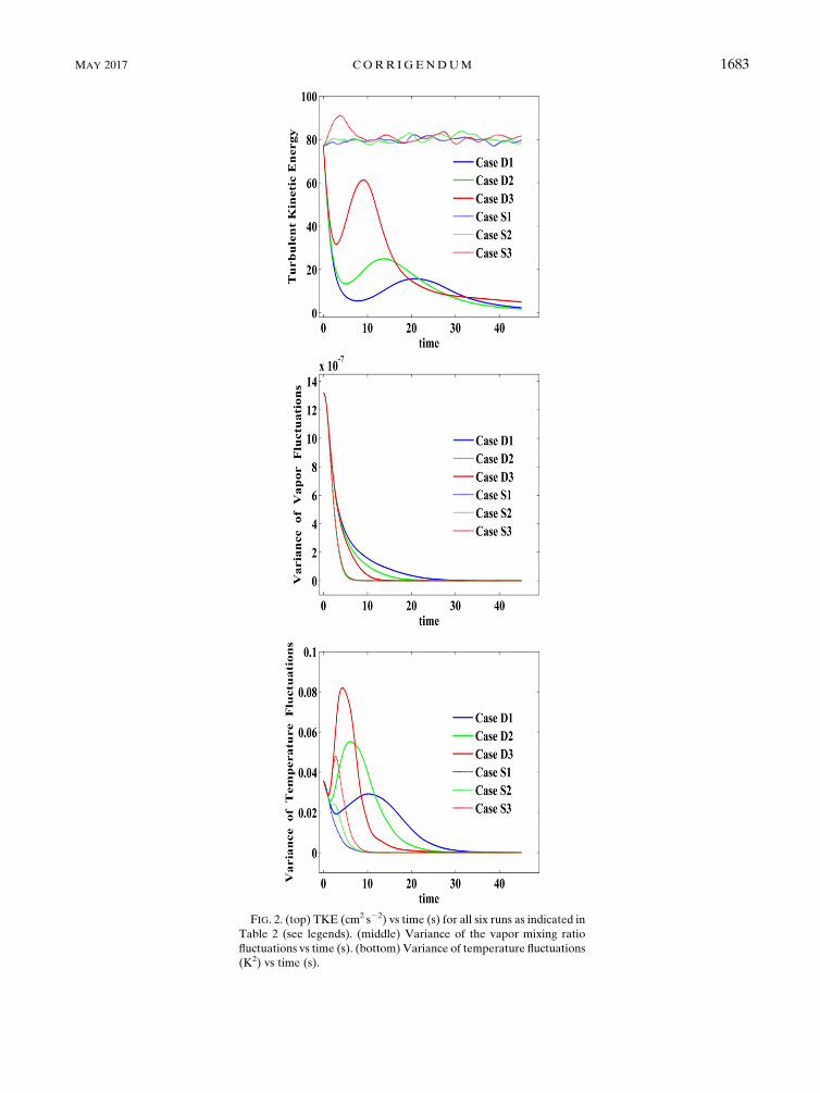
FIG. 2. (top) TKE (cm2 s22) vs time (s) for all six runs as indicated in

Table 2 (see legends). (middle) Variance of the vapor mixing ratio

fluctuations vs time (s). (bottom) Variance of temperature fluctuations

(K2) vs time (s).

MAY 2017 CORR IGENDUM 1683

FIG. 4. Mixing diagrams.Mean cubic radius andmixture fraction have been calculated in 16 equally sized sub-slabs

withLx,1# x#Lx,2. They are obtained by splitting the original cloud filament. Details of the four displayed cases are

given in Table 2.

1684 JOURNAL OF THE ATMOSPHER IC SC IENCES VOLUME 74

FIG. 5. As in Fig. 4, but for (left) 4 and (right) 16 equally sized sub-slabs . Both figures are for case D1 as indicated in

Table 2.

FIG. 6. Total number of droplets in the computational domain vs

time for all six cases. For cases S1 and D1, the equilibrium state has

a liquid water content of zero. All other cases end with finite liquid

water contents after transients have vanished; cases S3 and D3 show

little full evaporation, but S2 and D2 have significant loss of droplets.

In those intermediate cases, the number of fully evaporated droplets is

greater for the decaying turbulence. These contrasting results are in-

terpreted in the text. The time is measured in seconds.

MAY 2017 CORR IGENDUM 1685

FIG. 7. PDFs of the size distribution at different times (see legend) from t5 0.5, 1.0, 2.0, 5.0, 10.0, 20.0, and 30.0 s.

(top left) Case S1 and (top right) case D1. (bottom left) Case S3 and (bottom right) case D3 (see Table 2). The two

extreme cases are shown in order to illustrate microphysical response under conditions favoring inhomogeneous

response in (top) and homogeneous response in (bottom).

1686 JOURNAL OF THE ATMOSPHER IC SC IENCES VOLUME 74

FIG. 8. PDFs of the supersaturation along the Lagrangian droplet trajectories at the different times (see legend) as

in Fig. 7. (top left) Case S1 and (top right) case D1. (bottom left) Case S3 and (bottom right) case D3 (Table 2). The

two extreme cases are shown in order to illustrate microphysical response under conditions favoring inhomogeneous

response in (top) and homogeneous response in (bottom).Data are for cases and times as in Fig. 7. PDFs are obtained

for all particles, including evaporated droplets.

MAY 2017 CORR IGENDUM 1687