LAGRANGE METHOD IN SHAPE OPTIMIZATION FOR A CLASS OF … · LAGRANGE METHOD IN SHAPE OPTIMIZATION...

LAGRANGE METHOD IN SHAPE OPTIMIZATION FOR A CLASSOF NON-LINEAR PARTIAL DIFFERENTIAL EQUATIONS: A

MATERIAL DERIVATIVE FREE APPROACH ∗

KEVIN STURM†

Abstract. In this paper a new theorem is formulated which allows a rigorous proof of the shapedifferentiability without the usage of the material derivative; the domain expression is automaticallyobtained and the boundary expression is easy to derive. Furthermore, the theorem is applied to acost function which depends on a quasi-linear transmission problem. Using a Gagliardo penalizationthe existence of optimal shapes is established.

Key words. Lagrange method, shape derivative, non-linear PDE, material derivative

AMS subject classifications. 49Q10, 49Q12

1. Introduction. A map defined on a set of subsets of Rd is called shape func-tion. The study of these functions is the main topic of shape optimization. Theconcept of derivative in Banach spaces does not apply to shape functions since thereis no immediate vector space structure on spaces of shapes. Nevertheless, it is possibleto introduce a derivative for a shape function called shape derivative. To be moreprecise, let a shape function J : Ξ → R, with Ξ ⊂ Ω : Ω ⊂ Rd be given andassume that it is shape differentiable, i.e., the limit

(1.1) dJ(Ω)[θ] = limt0

(J(Ωt)− J(Ω)) /t,

exists and θ 7→ dJ(Ω)[θ] is continuous and linear. Here, we defined Ωt := Φt(Ω), wherethe mapping Φt is the flow generated by the differentiable vector field θ : Rd → Rd

with compact support. The structure theorem for shape functions on open domainsΩ ⊂ Rd of class Ck+1 is due to Zolesio [18] in 1979 and not to the Hadamard evenif the theorem is often called Hadamard structure theorem. It states that the shapederivative in an open domain Ω of class Ck+1 is a distribution on the boundaryΓ := ∂Ω that only depends on the normal part θn := θ · n of the vector field θ.Moreover, if the boundary Γ is smooth enough, the shape derivative can often bewritten in the form

(1.2) dJ(Ω)[θ] =

∫Γ

g θnds,

where g ∈ L1(Γ) is an integrable function. We call the integral over the boundary Γin (1.2) boundary expression of the shape derivative.

There are at least four ways to prove the existence of (1.1) when the cost functionis constrained by a partial differential equation (PDE): material derivative method(also called “chain rule approach”) [17], minimax formulation by [9], Cea’s Lagrangemethod introduced in [4] and rearrangement method introduced in [12].

As a byproduct of the proof of the existence of the shape derivative (1.1), oneusually gets the following expression

(1.3) dJ(Ω)[θ] =

∫Ω

F (θ, ∂θ, ∂2θ, . . .) dx,

∗This work was partially supported by the DFG Research Center Matheon†Weierstrass Institute, Berlin, ([email protected]).

1

2 LAGRANGE METHOD IN SHAPE OPTIMIZATION

where F is some function acting on θ and its derivatives. Under some smoothnessassumptions on the boundary of the domain Ω and the regularity of the solution ofthe underlying PDE, this expression can be brought by partial integration into theform (1.2). In most cases, the domain expression (1.3) can be derived without anyfurther regularity assumption on the PDE or the domain. In this sense the domainexpression is more general than the boundary expression.

The material derivative method analyzes the differentiability of the PDE withrespect to the domain. The material derivative is introduced to derive the shapedifferentiability, but it is not present in the final formula of the shape derivative.

Cea’s Lagrange method incorporates the PDE constraints in a Lagrangian andassumes that the shape derivatives of the PDE and the adjoint equation exist. Whilethe material derivative method gives a rigorous proof of the differentiability of theshape function, this is different for Cea’s Lagrange method. There are examples (see[15]), where Cea’s Lagrange method fails.

A theorem on the differentiability of a minimax in the infinite dimensional settingwas given by [6] and later applied to shape optimization by [8, Theorem 3, p. 842].This latter theorem provides a rigorous way to prove shape differentiability under theassumption that the corresponding Lagrangian has saddle points. Also in [8] anothertheorem was proved that requires no saddle point assumption. Nevertheless, thistheorem is not directly applicable and one has to go to a dual problem and require asaddle point assumption. We also refer the reader to [7, p. 93, Theorem 3], where atheorem is presented that does not use a saddle point assumption, but which is notapplicable for Lagrangian functionals.

Finally, the recently introduced rearrangement method of [12] bypasses the mate-rial derivative by some Holder continuity of the domain-solution mapping plus a firstorder expansion of the state equation and the cost function, which is assumed to beof order two. This method is applicable to many elliptic partial differential equations.

We would like to have a criterion when the minimax of the Lagrangian is differ-entiable without going to a dual problem or any saddle point assumption. Moreover,we wish to establish a theorem with very mild and fairly simple assumptions on thecost function and the state equation. This paper presents a novel approach to thedifferentiability of the minimax of a Lagrangian that is an utility function plus a lin-ear penalization of the state equation. Its originality is to replace the usual adjointstate equation by an averaged adjoint state equation. When compared to the formertheorems by [8, Theorem 3, p. 842], [7, Theorem 3, p. 93] and [6], all the hypothesesare now verified for a Lagrangian functional without going to the dual problem andany saddle point assumption. It relaxes the classical continuity assumptions on thederivative of the Lagrangian involving both the state and adjoint state to continuityassumptions that only involve the averaged adjoint state. This result opens new hori-zons not only for the shape calculus but also probably in mathematical programmingand optimal control (the maximum principle). Nevertheless, this is beyond the scopeof the present paper.

The main contributions of the paper are:

1. Novel approach to the rigorous computation of first order optimality condi-tions for equality constrained optimization problems without using the dif-ferentiability of the control-solution operator.

2. Application of the theorem to a cost function constrained by a quasi-lineartransmission problem. In particular, it is shown:(a) the existence of optimal shapes by a Gagliardo penalization,

KEVIN STURM 3

(b) the existence of the shape derivative and a formula for the boundary anddomain expression.

The structure of the paper:Section 2, the material method, a modification of Cea’s Lagrange method, the

minimax formulation and the rearrangement method are briefly discussed and a mo-tivation for our main result is given. Moreover, the reason why Cea’s Lagrange methodis not always applicable is explained and a solution is provided.

Section 3, we make some general assumptions and state then the main theorem.We prove that the new theorem allows an efficient computation of the shape derivativewithout using the material derivative or more generally without differentiating thecontrol-state operator.

Section 4, the results from Section 3 are applied to a non-linear transmissionproblem. For the presented example an application of the material derivative method(i.e. the strong material derivative) is not possible due to the lack of regularity.Finally, we present a minimization problem with penalization and show that theassociated cost function is shape differentiable.

2. Motivation and preliminaries. First we give some basic definitions andintroduce notations. Then we give a motivation for the main result, which is provedin the next section.

2.1. Notations and definitions. Let E and F be Banach spaces and U ⊂ E anopen subset. We denote by C(U ;F ) the space of all continuous functions f : U → F .The space C(U ;F ) comprises all continuous f : U → F and is endowed with the norm‖f‖C(U ;F ) := supx∈U ‖f(x)‖F < ∞. We call a function f : U → F differentiable in

x ∈ U if it is Frechet differentiable at x and denote the derivative by ∂f(x). Thefunction is called differentiable if it is differentiable at every point x ∈ U . For k ≥ 1,the space of all k-times continuously differentiable functions f : U → F is denotedby Ck(U ;F ). The Gateaux derivative of f : U → F at x ∈ U in direction v ∈ Eis denoted by ∂vf(x). For a differentiable function f : U → F , we have ∂f(x)(v) =∂vf(x) for all x ∈ U and v ∈ E. If we only consider the directional derivative of f ,we write df(x; v) or df(x)(v) to indicate the directional derivative at x in directionv. For a function f : E1 × · · · × En → F , where E1, . . . , En are Banach spaces, wealso write ∂xkf(x1, . . . , xn)(xk) := ∂(0,...,xk,...,0)f(x1, . . . , xn), where k, l ≥ 0 are suchthat 1 ≤ k ≤ n < ∞. In the case F = R and E being a Hilbert space, we havethat ∂f(x) : E → R is a continuous, linear mapping and therefore we may writeby the Riesz representation theorem ∂f(x)(v) = v · v for some element v ∈ E (“ · “being the inner product on E). The vector v is then called gradient of f at x anddenoted by ∇f(x). For p ≥ 1, the space of all measurable functions f : Ω → R for

which ‖f‖Lp(Ω) :=(∫

Ω|f |p dx

)1/p< ∞ is denoted by Lp(Ω). The space of functions

of bounded variations on D are denoted by BV (D). For the right sided limit limt→0t>0

we write limt0.Let d ∈ N+. Assume that D ⊂ Rd is an bounded domain with Lipschitz bound-

ary. For any k ≥ 1, we define the space

CkD(Rd) := θ ∈ Ck(Rd; Rd) : supp(θ) ⊂ D.

The flow of a vector field θ ∈ CkD(Rd) is defined for each x0 ∈ D by Φθt (x0) := x(t),where x : [0, τ ]→ Rd solves

x(t) = θ(x(t)) in (0, τ), x(0)= x0.


In the sequel, we write Φt instead of Φθt . For an invertible matrix L ∈ Rd,d,we have (L−1)T = (LT )−1 and therefore we define L−T := (L−1)T . Henceforth, thefollowing abbreviations are frequently used in the paper

(2.1) ξ(t) := det(∂Φt), A(t) := ξ(t)∂Φ−1t ∂Φ−Tt , B(t) := ∂Φ−Tt .

Note that by the chain rule (∂(Φ−1t )) Φt = (∂Φt)

−1 =: ∂Φ−1t . We use the notation

θn := θ · n for the normal component of the vector field θ, where n ∈ Rd such that|n| = 1. Let us recall some useful facts about the transformation Φt associated withthe vector field θ ∈ CkD(Rd).

Lemma 2.1. Fix k ≥ 1. Let θ ∈ CkD(Rd) be a given vector field and Φt its flow.1. Assume p > 1 and f ∈ Lp(R

d). Then limt0 ‖f Φ−1t − f‖Lp(Rd) =

limt0 ‖f Φt − f‖Lp(Rd) = 0.

2. Let f ∈ H1(Rd). Then limt0 ‖f Φt − f‖H1(Rd) = 0.3. The jacobian ξ(t) is differentiable from the right side with derivative

limt0

(ξ(t)− 1)/t = div (θ) in C(D).

4. The limit limt0(A(t)−A(0))/t exists in C(D; Rd,d) and is given by

(2.2) A′(0) = div (θ)Id,d − ∂θ − ∂θT .

5. The derivative A′ is continuous, i.e., A′(t)→ A′(0) in C(D; Rd,d).Proof. See [9, p.527], [17] and [12].Definition 2.2 (Eulerian semi-derivative). Suppose we are given a shape func-

tion J : Ξ → R on the set Ξ ⊂ Ω| Ω ⊂ D. Denote by Φt : D ×R → D the flowgenerated by the vector field θ ∈ CkD(Rd), where k ≥ 1 and set Ωt := Φt(Ω). Then theEulerian semi-derivative of J at Ω ⊂ D in the direction θ is defined as the limit(if it exists)

dJ(Ω)[θ] := limt0

1

t(J(Ωt)− J(Ω)) .

In general, the derivative dJ(Ω)[θ] can be non-linear in θ.Definition 2.3. Let Ω ⊂ D and D ⊂ Rd be open sets. The function J is said to

be shape differentiable at Ω if the Eulerian semi-derivative dJ(Ω)[θ] exists for allθ ∈ C∞D (Rd) and the map θ 7→ dJ(Ω)[θ] : C∞D (Rd)→ R, is linear and continuous.

Finally, we state the following theorem from [9, pp. 483-484], which will laterallow us to calculate the boundary expression of the shape derivative.

Theorem 2.4. Let θ ∈ CkD(Rd), where k ≥ 1. Fix τ > 0 and let ϕ ∈C(0, τ ;W 1,1

loc (Rd))∩C1(0, τ ;L1loc(R

d)) and an bounded domain Ω with Lipschitz bound-ary Γ be given. The right sided derivative of the function

f(t) :=

∫Ωt

ϕ(t) dx

at t = 0 is given by

d+

dtf(0) =

∫Ω

ϕ′(0) dx+

∫Γ

ϕ(0) θn dx,

where d+

dt f(0) := limt0(f(t)− f(0))/t.

KEVIN STURM 5

2.2. Motivation. In order to motivate the main theorem presented in Section 3,we consider simple model problem. Let Ω ⊂ Rd be an open, bounded set with smoothboundary ∂Ω. We consider the state equation

−∆u = f, in Ω,

u = 0, on ∂Ω,(2.3)

where f : Rd → R is a smooth function. The function u : Ω→ R is called state. Tosimplify the exposition, we choose as objective function

(2.4) J(Ω) :=

∫Ω

|u− ud|2 dx,

where ud ∈ H2(Rd) is given and | | denotes the absolute value. We call u ∈ H10 (Ω) a

weak solution of (2.3) if

(2.5)

∫Ω

∇u · ∇ψ dx =

∫Ω

fψ dx, for all ψ ∈ H10 (Ω).

We aim to calculate the shape derivative of (2.4). For this purpose, we consider theperturbed cost function and apply a change of variables to obtain

(2.6) J(Ωt) =

∫Ω

ξ(t)|ut − ud Φt|2 dx,

where ut := ut Φt and ut denotes the weak solution of (2.5) on the domain Ωt :=Φt(Ω). To study the differentiability of (2.6), we can study the function t 7→ ut. The

limit u := limt0ut−ut is called strong material derivative if we consider this limit

in the norm convergence in H10 (Ω) and weak material derivative if we consider the

weak convergence in H10 (Ω).

Henceforth, we make use of the following convention. Whenever a function f :D → R on the hold-all D is given, we denote by f t := Ψt(f) := f Φt the ’pull-back’of f and define also its inverse Ψ−1

t (ϕ) := Ψt(f) := f Φ−1t .

It is readily verified by considering the equation (2.5) on Ωt and an applicationof the change variables Φt(x) = y that ut satisfies

(2.7)

∫Ω

A(t)∇ut · ∇ψ dx =

∫Ω

ξ(t)f tψ dx, for all ψ ∈ H10 (Ω),

where we used the notation from (2.1). By standard regularity theory, we may assumethat the solution belongs to H2(Ω) ∩H1

0 (Ω). Note that the solution of the previousequation is the unique minimum of the strongly convex energy E : [0, τ ]×H1

0 (Ω)→ Rwith respect to the second argument

(2.8) E(t, ϕ) :=1

2

∫Ω

ξ(t)|B(t)∇ϕ|2 dx−∫

Ω

ξ(t)f tϕdx.

It can be shown that t 7→ ut : [0, τ ]→ H10 (Ω) is differentiable, see for instance [17].

Remark 1. We would like to stress that the proof of the differentiability oft 7→ ut in the appropriate function space is not obvious in general and may involveheavy tools from analysis such as the implicit function theorem. In many situationsthe implicit function theorem is not applicable. For other non-linear problems such asthe Navier-Stokes equations, we refer the reader to the monograph [16].


Without going into further details, we may show by introducing the adjoint equa-tion

(2.9) Find p ∈ H10 (Ω) :

∫Ω

∇p·∇ψ dx = −2

∫Ω

(u−ud)ψ dx, for all ψ ∈ H10 (Ω),

and verifying that the material derivative u satisfies

(2.10)

∫Ω

∇u · ∇ψ dx+

∫Ω

A′(0)∇u · ∇ψ dx =

∫Ω

div (θ)fψ dx+

∫Ω

∇f · θψ dx,

that the shape derivative is given by

dJ(Ω)[θ] =

∫Ω

div (θ)|u− ud|2 dx−∫

Ω

2(u− ud)∇ud · θ dx

+

∫Ω

A′(0)∇u · ∇p dx−∫

Ω

div (θ)fp dx−∫

Ω

∇f · θp dx.(2.11)

Note that the domain expression already makes sense when u, p ∈ H10 (Ω). According

to the structure theorem (cf. [9, p.479-481, Corollary 1]), the previous equation canbe written as an boundary integral over ∂Ω depending only on the normal part ofthe perturbation field θ. This can be accomplished by integrating by parts in (2.11)or by introducing the shape derivative of the state u. However, this requires higherregularity of u and p. We refer the reader to [17] for the usage of the shape derivativemethod.

We point out that there is no material derivative u in the final expression (2.11).This suggests that there might be a way to obtain this formula without the compu-tation of u. Indeed, instead of computing the material derivative and deriving anequation for this derivative, one may also introduce the function

(2.12) G(t, ϕ, ψ) =

∫Ω

ξ(t)|ϕ− utd|2 dx+

∫Ω

A(t)∇ϕ · ∇ψ dx−∫

Ω

ξ(t)f tψ dx.

It is evident that the shape differentiability of J is equivalent to the differentiabilityof

(2.13) t 7→ g(t) := G(t, ut, ψ),

from the right in 0 for any ψ, where ut solves (2.7). Note that we have the relation

(2.14) G(t, ut, ψ) = minϕ∈H1

0 (Ω)sup

ψ∈H10 (Ω)

G(t, ϕ, ψ)

for any ψ ∈ H10 (Ω), therefore the differentiability of g can be obtained by differentiat-

ing a minimax of a Lagrangian with respect to a parameter. Notice that the relation(2.14) only holds when the PDE has a unique solution. One way to prove the differ-entiability of g under the assumption that G is convex as function ϕ 7→ G(t, ϕ, ψ) forall t ∈ [0, τ ] and ψ provides the Theorem of Correa-Seeger [8]. The recently proposedrearrangement method of [12] provides another way to prove the differentiability of(2.13) without using the material derivative. For non-linear problems the rearrange-ment requires a first order expansion of the PDE with respect to the unknown as well

KEVIN STURM 7

as the cost function such that the remainder converges towards zero with order two.1

We refer the reader to [12] and [13] for more details on this method and also point outthe paper [14], where second order shape derivatives are computed by this method.

Finally, let us remark that if the cost function J is the energy of the PDE, i.e.J(Ωt) = E(t, ut) then it is well-known that J may be differentiated without using thematerial derivative by only employing the continuity of t 7→ ut, see e.g. [9, p.524,Theorem 2.1]. In this case it is not nessacary to introduce an adjoint equation andthe shape derivative involves only the state u.

2.3. Cea’s classical Lagrange method and a modification. Let the func-tion G be defined by (2.12). Assume that G is sufficiently differentiable with respectto t, ϕ and ψ. Additionally, assume that the strong material derivative u exists inH1

0 (Ω). Then by invoking the chain rule we may calculate as follows

(2.15) dJ(Ω)[θ] =d

dt(G(t, ut, p))|t=0 = ∂tG(t, u, p)|t=0︸︷︷︸

shape derivative

+ ∂ϕG(0, u, p)(u)︸︷︷︸adjoint equation

,

and due to u ∈ H10 (Ω) it implies dJ(Ω)[θ] = ∂tG(t, u, p)|t=0. Therefore, we can follow

the lines of the calculation of the previous section to obtain the boundary and domainexpression of the shape derivative. In the original work [4], it was calculated as follows

(2.16) dJ(Ω)[θ] = ∂ΩL(Ω, u, p) + ∂ϕL(Ω, u, p)(u′) + ∂ψL(Ω, u, p)(p′),

where ∂ΩL(Ω, u, p) := limt0(L(Ωt, u, p)−L(Ω, u, p))/t. Then it was assumed that u′

and p′ belong toH10 (Ω), which has as consequence that ∂ϕL(Ω, u, p)(u′) = ∂ψL(Ω, u, p)(p′) =

0. Thus (2.16) leads to the wrong formula

dJ(Ω)[θ] =

∫Γ

(|u− ur|2 + ∂nu ∂np) θn ds.

This can be fixed by noting that u′ = u−∇u ·θ and p′ = p−∇p ·θ with u, p ∈ H10 (Ω):

dJ(Ω)[θ] = ∂ΩL(Ω, u, p)− ∂ϕL(Ω, u, p)(∇u · θ)− ∂ψL(Ω, u, p)(∇p · θ),

which gives the correct formula. Note that we do not claim that the Lagrange methodto calculate the volume or boundary expression is always applicable, but it is appli-cable under the described assumptions also for non-linear problems. For a particularproblem one has to carefully check the assumptions. One example where the de-scribed method is not working is the p-Laplacian, where it is known that the materialderivative only belongs to some weighted Sobolev space and not to the solution spaceof the PDE.

3. Avoiding the material derivative. We have seen in the previous sectionthat the shape derivative of a PDE constrained shape optimization problem can beexpressed as the derivative of the function g(t) := G(t, ut, ψ), at t = 0. The rear-rangement method and the Theorem of Correa-Seeger show that the differentiation ofg does not require the differentiation of t 7→ ut, in general. In this section, we presenta novel theorem to prove the differentiability of g, which extends the Theorem ofCorrea-Seeger for the special class of Lagrangians.

1By a first order expansion with remainder of order two of a function f : E → R, where (E, ‖ · ‖)is a Banach space, we mean that f satisfies

f(x)− f(y)− df(x;x− y) ∈ O(‖x− y‖2).


3.1. Differentiability of the Lagrangian without material derivatives.Let the Banach spaces E,F and a number τ > 0 be given. Consider a function

G : [0, τ ]× E × F → R, (t, ϕ, ψ) 7→ G(t, ϕ, ψ).

We introduce the solution set of the state equation

(3.1) E(t) := u ∈ E| dψG(t, u, 0; ψ) = 0 for all ψ ∈ F.

Let us introduce the following hypothesis.Assumption (H0).(i) For all t ∈ [0, τ ], ut ∈ E(t), u0 ∈ E(0) and p ∈ F the mapping

[0, 1]→ R : s 7→ G(t, sut + s(ut − u0), p)

is absolutely continuous. This implies that for almost all s ∈ [0, 1] the deriva-tive dϕG(t, u0 + s(ut − u0), p;ut − u0) exists and in particular

G(t, ut, p)−G(t, u0, p) =

∫ 1

0

dϕG(t, sut + (1− s)u0, p;ut − u0) ds.

(ii) For all t ∈ [0, τ ], ϕ ∈ E, p ∈ F , ut ∈ E(t) and u0 ∈ E(0)

dϕG(t,sut + (1− s)u0, p;ϕ)

exists and s 7→ dϕG(t, sut + (1− s)u0, p;ϕ) belongs to L1(0, 1).(iii) For every (u, t) ∈ E × [0, τ ] the mapping F → R : p 7→ G(t, u, p) is affine-

linear.Introduce for t ∈ [0, τ ], ut ∈ E(t) and u0 ∈ E(0) the following set

(3.2) Y (t, ut, u0) :=

q ∈ F | ∀ϕ ∈ E :

∫ 1

0

dϕG(t, sut + (1− s)u0, q; ϕ) ds = 0

,

which is called solution set of the averaged adjoint equation with respect to t,ut andu0. For t = 0, we set Y (0, u0) := Y (t, ut, u0), which coincides with the solution set ofthe usual adjoint state equation

(3.3) Y (0, u0) :=q ∈ F | dϕG(0, u0, q; ϕ) = 0 for all ϕ ∈ E

.

We call any p ∈ Y (0, u0) an adjoint state. In the most general situation, we define fort ∈ [0, τ ], ut ∈ E(t) and u0 ∈ E(0) the set

(3.4) Y (t, ut, u0) :=q ∈ F | G(t, ut, q)−G(t, u0, q) = 0

.

Note under the assumption (H0), we have Y (t, ut, u0) ⊂ Y (t, ut, u0) for all t ∈ [0, τ ],ut ∈ E(t), u0 ∈ E(0). In particular, we have Y (0, u0, u0) = F .

We now prove a theorem which enables us to calculate the shape derivative with-out the knowledge of the material derivative u. The key ingredient is the introductionof the set (3.2).

Theorem 3.1. Let the linear vector spaces E and F , the real number τ > 0, andthe function

G : [0, τ ]× E × F → R, (t, ϕ, ψ) 7→ G(t, ϕ, ψ),

be given. Let Assumption (H0) and the following conditions be satisfied.

KEVIN STURM 9

(H1) For all t ∈ [0, τ ] and all (u, p) ∈ E(0)× F the derivative ∂tG(t, u, p) exists.(H2) For all t ∈ [0, τ ], E(t) is nonempty and single-valued. For all t ∈ [0, τ ],

ut ∈ E(t) and u0 ∈ E(0), the set Y (t, ut, u0) is nonempty and single-valued.(H3) Let u0 ∈ E(0) and p0 ∈ Y (0, u0). For any sequence (tn)n∈N of non-negative

real numbers converging to zero, there exist a subsequence (tnk)k∈N, elementsutnk ∈ E(tnk) and ptnk ∈ Y (tnk , u

tnk , u0) such that

limk→∞t0

∂tG(t, u0, ptnk ) = ∂tG(0, u0, p0).

Let us pick any ψ ∈ F . Then letting t ∈ [0, τ ], ut ∈ E(t), u0 ∈ E(0) and p0 ∈ Y (0, u0),we conclude

(3.5)d

dt(G(t, ut, ψ))|t=0 = ∂tG(0, u0, p0).

Proof. Step 1: Let t ∈ [0, τ ], ut ∈ E(t), u0 ∈ E(0) and pt ∈ Y (t, ut, u0), p0 ∈Y (0, u0) be given. We will show that there exist a ηt ∈ (0, 1) such that

G(t, ut, ψ)−G(0, u0, ψ) = t∂tG(ηtt, u0, pt),(3.6)

for all ψ ∈ F . Write

G(t, ut, ψ)−G(0, u0, ψ) = G(t, ut, pt)−G(0, u0, p0)

= G(t, ut, pt)−G(t, u0, pt) +G(t, u0, pt)−G(0, u0, pt)

(3.7)

for all ψ ∈ F , where we used G(0, u0, pt) − G(0, u0, p0) = 0, since p 7→ G(t, u, p) isaffine linear. By hypothesis (H1), we find for each t ∈ [0, τ ] a number ηt ∈ (0, 1) suchthat

(3.8) G(t, u0, pt)−G(0, u0, pt) = t∂tG(ηtt, u0, pt).

Now using part (i) and (ii) of hypothesis (H0), we obtain pt ∈ Y (t, ut, u0) and thusplugging (3.8) into (3.7), we recover (3.6).Step 2: For arbitrary ψ ∈ F , we show that limt0 δ(t)/t exists, where δ(t) :=

G(t, ut, ψ) − G(0, u0, ψ). To do so it is sufficient to show that lim inft0δ(t)t =

lim supt0δ(t)t . By definition of the lim inf, there is a sequence (tn)n∈N such that

limn→∞

δ(tn)/tn = lim inft0

δ(t)/t =: dδ(0).

Now let u0 ∈ E(0) and p0 ∈ Y (0, u0). Recall that δ(t)/t = ∂tG(ηtt, u0, pt). Owing to

(H3), for any sequence (tn)n∈N converging to zero, i.e., tn → 0 as n→∞, there existsa subsequence (tnk)k∈N, elements utnk ∈ E(tnk) and ptnk ∈ Y (tnk , u

tnk , u0) such that

limk→∞t0

∂tG(t, u0, ptnk ) = ∂tG(0, u0, p0).

Thus we conclude

dδ(0) = limn→∞

∂tG(ηtntn, u0, ptn) = lim

k→∞∂tG(ηtnk tnk , u

0, ptnk )

= ∂tG(0, u0, p0).(3.9)


Completely analogous, we may show for dδ(0) := lim supt0 δ(t)/t that

(3.10) dδ(0) = ∂tG(0, u0, p0)

Combining (3.9) and (3.10), we obtain dδ(0) = ∂tG(0, u0, p0) = dδ(0), which shows

that limt0δ(t)t = ∂tG(0, u0, p0). Since ψ ∈ F was arbitrary, we finish the proof.

Remark 2. In concrete applications the conditions (H0)-(H3) have the followingmeaning.

(i) Condition (H0) ensures that we can apply the fundamental theorem of calculusto G with respect to the primal variable. Condition (H1) allows an applicationof the mean value theorem with respect to t. Note that the assumption (H0)is much milder than Frechet differentiability.

(ii) Condition (H2) ensures that the state equation and the perturbed state equa-tion has a unique solution. The set Y (t, ut, u0) can be understood as thesolution of some averaged adjoint state equation.

(iii) Condition (H3) can be verified by showing that pt converges weakly to p0

and that (t, ψ) 7→ G(t, u0, ψ) is weakly continuous. Note that there is noassumption on the convergence of ut ∈ E(t) to u0 ∈ E(0), but in applicationswe need the convergence ut → u0 to prove pt → p0 in some topologies.

(iv) The set E(t) corresponds to the solution of the state equation on the perturbeddomain Ωt brought back to the fixed domain Ω.

3.2. Possible generalizations. We can consider a weaker averaged equationand thus weaken the conditions (i),(ii) of assumption (H0). We may write G as

G(t, ϕ, ψ) = f(t, ϕ) + l(t, ϕ, ψ),

for two functions f : [0, τ ]×E → R and l : [0, τ ]×E×F → 0, where the function l islinear in p. Now it is sufficient to require that l satisfies assumption (H0) (G replacedby l) and for f we need: for all t ∈ [0, τ ], ut ∈ E(t), u0 ∈ E(0) the function

[0, τ ]→ R : s 7→ f(t, sut + (1− s)u0)

is differentiable. Under these assumptions, we conclude by the mean value theoremthat there exists s′ ∈ [0, τ ] depending on t such that

(3.11) f(t, ut)− f(t, u0) = dϕf(t, s′ut + (1− s′)u0;ut − u0)

and in particular

G(t, ut, p)−G(t, u0, p) =

∫ 1

0

dϕl(t, sut + (1− s)u0, p;ut − u0) ds

+ dϕf(t, s′ut + (1− s′)u0;ut − u0).

Now assume that for all t ∈ [0, τ ], ut ∈ E(t), u0 ∈ E(0), s′ ∈ (0, 1) and for all u ∈ E

dϕf(t, s′ut + (1− s′)u0; u)

exists. Then instead of considering the averaged equation, we could consider themodified averaged equation: Find pt ∈ F such that

(3.12)

∫ 1

0

dϕl(t, sut + (1− s)u0, pt; u) ds+ dϕf(t, s′ut + (1− s′)u0; u) = 0

KEVIN STURM 11

for all u ∈ E. Since s′ (defined by (3.11)) depends on t, the set Y (t, ut, u0) has to bereplaced by

Y (t, ut, u0) := q ∈ F : q solves (3.12) with s′ such that (3.11).

Then we can follow the lines of the proof of Theorem 3.1 with the mentioned changes.Since in applications f will be the cost function, this remark means that we only needthe cost function to be directional differentiable without continuity. Nevertheless, toidentify the limit p0 we need some continuity to pass to the limit t 0 in (3.12).Using the Henstock–Kurzweil integral in (3.12) (cf. [3]), we may even weaken theabsolute continuity of s 7→ l(t, sut + (1− s)u0, p) (p ∈ F ) to differentiability, since forthis integral the fundamental theorem is satisfied for merely differentiable functions.

4. A quasi-linear transmission problem. As an application of Theorem 3.1,we investigate a non-linear transmission problem and use it to compute the shapederivative. We associate with the transmission problem a minimization problem. Toachieve the well-posedness of the minimization problem a Gagliardo regularization isused. The considered model constitutes a generalization of the electrical impedancetomography (EIT) problem, which can be found in [1].

4.1. The problem setting. Let D ⊂ Rd be a bounded domain with Lipschitzboundary ∂D and Ω ⊂ D be a measurable subset. We set Ω+ := Ω, Ω− := D \ Ω+

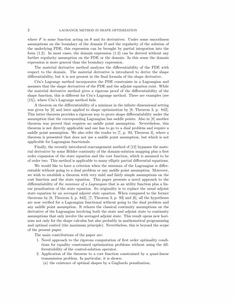
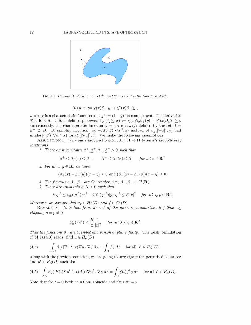
and Γ := ∂Ω+ ∩ ∂Ω−. An example of a domain D with subset Ω+ ⊂ D is depicted inFigure 4.1. We consider for p ∈ (1,∞) and 0 < s < 1/p the cost function

(4.1) J(Ω) := J1(Ω) + αJ2(Ω) :=

∫D

|u(Ω)− ur|2 dx+ α|χΩ|pW sp (D)

constrained by the equations

−div (β+(|∇u+|2)∇u+) = f+ in Ω+

−div (β−(|∇u−|2)∇u−) = f− in Ω−

u = 0 on ∂D

(4.2)

complemented by transmission conditions on Γ

(4.3) [u]Γ = 0 and β+(|∇u+|2)∂nu+ = β−(|∇u−|2)∂nu

−.

Here, n := n+ denotes the outward unit normal vector along the interface Γ = ∂Ω+ ∩∂Ω−. We denote by n− := −n = −n+ the outward unit normal vector of Ω−. Thebracket

[φ]Γ (x) := limz→x,z∈Ω+

φ(z)− limz→x,z∈Ω−

φ(z)

will indicate the jump of a function φ across Γ at x ∈ Γ. For a given functionϕ : D → R, we write ϕ+ for the restriction ϕ|Ω+ : Ω+ → R and likewise ϕ− forϕ|Ω− : Ω− → R. The penalty term in (4.1) is called Gagliardo semi-norm anddefined by

|χΩ|pW sp (D) :=

∫D

∫D

|χΩ(x)− χΩ(y)|p

|x− y|d+spdx dy.

For later usage it is convenient to introduce the functions βχ : R×R→ R


Ω+

Γ

D

Ω−

n+

Fig. 4.1. Domain D which contains Ω+ and Ω−, where Γ is the boundary of Ω+.

βχ(y, x) := χ(x)β+(y) + χc(x)β−(y),

where χ is a characteristic function and χc := (1−χ) its complement. The derivativeβ′χ : R × R → R is defined piecewise by β′χ(y, x) := χ(x)∂yβ+(y) + χc(x)∂yβ−(y).Subsequently, the characteristic function χ = χΩ is always defined by the set Ω =Ω+ ⊂ D. To simplify notation, we write β(|∇u|2, x) instead of βχ(|∇u|2, x) andsimilarly β′(|∇u|2, x) for β′χ(|∇u|2, x). We make the following assumptions.

Assumption 1. We require the functions β+, β− : R→ R to satisfy the followingconditions.

1. There exist constants β+, β+, β−, β− > 0 such that

β+ ≤ β+(x) ≤ β+, β− ≤ β−(x) ≤ β− for all x ∈ Rd.

2. For all x, y ∈ R, we have

(β+(x)− β+(y))(x− y) ≥ 0 and (β−(x)− β−(y))(x− y) ≥ 0.

3. The functions β+, β− are C1-regular, i.e., β+, β− ∈ C1(R).4. There are constants k,K > 0 such that

k|η|2 ≤ β±(|p|2)|η|2 + 2β′±(|p|2)|p · η|2 ≤ K|η|2 for all η, p ∈ Rd.

Moreover, we assume that ur ∈ H1(D) and f ∈ C1(D).Remark 3. Note that from item 4 of the previous assumption it follows by

plugging η = p 6= 0

β′±(|η|2) ≤ K

2

1

|η|2for all 0 6= η ∈ Rd.

Thus the functions β± are bounded and vanish at plus infinity. The weak formulationof (4.2),(4.3) reads: find u ∈ H1

0 (D)∫D

βχ(|∇u|2, x)∇u · ∇ψ dx =

∫D

fψ dx for all ψ ∈ H10 (D).(4.4)

Along with the previous equation, we are going to investigate the perturbed equation:find ut ∈ H1

0 (D) such that

(4.5)

∫D

βχ(|B(t)∇ut|2, x)A(t)∇ut · ∇ψ dx =

∫D

ξ(t)f tψ dx for all ψ ∈ H10 (D).

Note that for t = 0 both equations coincide and thus u0 = u.

KEVIN STURM 13

4.2. Existence of optimal shapes. We are interested in the question underwhich restriction on the characteristic functions a minimization of (4.1) admits asolution. We investigate the problem

(4.6) min J(χΩ) over χΩ ∈ BW sp (D),

where J(χΩ) := J(Ω) and J is given by (4.1). In the following, we use the notationX(D) to indicate the set of all characteristic functions χΩ defined by a Lebesquemeasurable set Ω ⊂ D. For every p ∈ (1,∞) and 0 < s < 1/p, we introduce the space

(4.7) BW sp (D) := χΩ : R→ R| χΩ ∈ X(D) and |χΩ|W s

p (D) <∞,

which is not empty since BV (D) ∩ L∞(D) ⊂ BW sp (D), see [9, p.253, Theorem 6.9.].

Compared with the perimeter2 PD(Ω) the function |χΩ|pW sp (D) provides a weaker regu-

larization. In particular, the regularization term and its shape derivative are domainintegrals. This makes the regularization favorable for numerical simulations. Alsonote that an open and bounded set Ω ⊂ Rd of class C2 has finite perimeter and thusχΩ ∈ BV (D) ∩ L∞(D), which implies χΩ ∈ BW s

p (D). We begin our investigationwith the study of the state equations (4.4) and (4.5).

Theorem 4.1. Let θ ∈ C2D(Rd) be a vector field and Φt its associated flow. Then

the equation (4.5) has for each t ∈ [0, τ ] and χ ∈ X(D) a unique solution in H10 (D).

Proof. Let Ω+ ⊂ D be measurable and define the measurable set Ω− := D \ Ω+.Then by definition D = Ω+ ∪ Ω−. Introduce the family of energy functionals

E(t, ϕ) :=

∫D

1

2[χ(x)ξ(t)h+(|B(t)∇ϕ(x)|2) + (1− χ(x))ξ(t)h−(|B(t)∇ϕ(x)|2)]+

+ ξ(t)f t(x)ϕ(x) dx,

(4.8)

where h± is the primitive of β± and given by

(4.9) h±(z) = c± +

∫ z

0

β±(s) ds,

for some constants c± ∈ R. We may choose c± = 0. We are going to show that theenergy E(t, ϕ) is convex with respect to ϕ. The first order directional derivative atϕ ∈ H1

0 (D) in direction ψ ∈ H10 (D) reads:

dE(t, ϕ;ψ) =

∫D

β(|B(t)∇ϕ|2, x)A(t)∇ϕ · ∇ψ dx−∫D

ξ(t)f tψ dx.

Note that the equation dE(t, ut;ψ) = 0 for all ψ ∈ H10 (D), conicides with equation

(4.5). We now prove that the second order directional derivative of E(t, ϕ) exists andis strictly coercive. Note that in order to prove the existence of the second orderdirectional derivative of E(t, ϕ), it is sufficient to show that for any u, ϕ, ψ ∈ H1

0 (D)

s 7→∫D

β(|B(t)∇(u+ sϕ)|2, x)A(t)∇(u+ sϕ) · ∇ψ dx(4.10)

2Recall that the perimeter of a set Ω ⊂ Rd is defined as PD(Ω) :=sup

ϕ∈C1D

(Rd)

‖ϕ‖L∞(D)<∞

∫Rd div (ϕ)χΩdx.


is continuously differentiable on R. Moreover for this it is sufficient to show that

s 7→∫

Ω±

β±(|B(t)∇(u+ sϕ)|2, x)A(t)∇(u+ sϕ) · ∇ψ dx(4.11)

is differentiable on R. Put s 7→ αs(x) := |B(t)∇(u + sϕ)|2, then it is immediatethat the function γ±s (x) := β±(αs(x))A(t)∇(u(x)+sϕ(x)) ·∇ψ(x) is differentiable foralmost all x ∈ Ω±, respectively. The derivative in the respective domain Ω+ and Ω−(briefly Ω±) reads

d

dsγ±s (x) =β′±(|B(t)∇(u+ sϕ)|2)B(t)∇(u+ sϕ) ·B(t)∇uA(t)∇(u+ sϕ) · ∇ψ

+ β±(|B(t)∇(u+ sϕ)|2)A(t)∇ϕ · ∇ψ.

(4.12)

Using Assumption 1 item 4, we conclude that there exists a constant K > 0 such that

(4.13)d

dsγ±s (x) ≤ K|∇ϕ(x)||∇ψ(x)|, for almost every x ∈ Ω±, for all s ∈ R.

Since s 7→ ddsγ±s (x) is also continuous on R, we get by the fundamental theorem of

calculus

γ±s (x)− γ±s+h(x)

h=

1

h

∫ s+h

s

d

dsγ±s (x) ds′

(4.13)

≤ K|∇ϕ(x)||∇ψ(x)| for almost all x ∈ Ω±.

(4.14)

Note, that the constant K is independent of x and s. Thus we may apply Lebesque’stheorem of dominated convergence to show that (4.11) is indeed differentiable withderivative

d

ds

∫Ω±

β±(αs(x))A(t)∇(u+ sϕ) · ∇ψ dx

=

∫Ω±

β′±(αs(x))B(t)∇(u+ sϕ) ·B(t)∇ϕA(t)∇(u+ sϕ) · ∇ψ

+ β±(αs(x))A(t)∇ϕ · ∇ψ dx.

(4.15)

It is immediate from the previous expression that the derivative is continuous. Weconclude that d2E(t, ϕ;ψ,ψ) exists for all ϕ,ψ ∈ H1

0 (D) and t ∈ [0, τ ]. Moreover,using Assumption 1 item 4, we get that there is C > 0 such that

(4.16) d2ϕE(t, ϕ;ψ,ψ) ≥ C‖ψ‖2H1(D) for all ϕ,ψ ∈ H1

0 (D), and for all t ∈ [0, τ ].

In the next lemma, we prove the Lipschitz continuity of the mapping X(D) 3χ 7→ u(χ) ∈ H1

0 (D), where u(χ) denotes the weak solution of (4.4) and X(D) isendowed with the Lp(D)-norm (p > 1).

Lemma 4.2. Let γ > 0 be a real number. Assume that there exist C > 0 andε > 0 such that for every χ ∈ X(D) we have ‖u(χ)‖W 1,2+ε(Ω) ≤ C, where u = u(χ)solves (4.4). Then there is a constant C > 0 such that for all characteristic functionsχ1, χ2 ∈ X(D):

‖u(χ1)− u(χ2)‖H1(D) ≤ C‖χ1 − χ2‖L1+γ(D),

KEVIN STURM 15

where u(χ1) and u(χ2) are solution of the state (4.4).

Proof. Let p ∈ (1,∞) and 0 < s < 1/p. Let u(χ1) = u1 and u(χ2) = u2 besolutions in H1

0 (D) of (4.4) associated with the functions χ1, χ2 ∈ X(D). Then byboundedness of βχ1

and βχ2, we obtain

C1‖u1 − u2‖2H1(D) ≤∫D

βχ1(|∇u1|2, x)∇(u1 − u2) · ∇(u1 − u2) dx

=

∫D

(βχ2(|∇u2|2, x)− βχ1

(|∇u1|2, x))∇(u1 − u2) · ∇u2 dx

and also

C2‖u1 − u2‖2H1(D) ≤∫D

βχ2(|∇u2|2, x)∇(u1 − u2) · ∇(u1 − u2) dx

=

∫D

(βχ2(|∇u2|2, x)− βχ1(|∇u1|2, x))∇(u1 − u2) · ∇u1 dx.

Adding both inequalities yields with C := C1 + C2

C‖u1 − u2‖2H1(D) ≤∫D

(βχ2(|∇u2|2, x)− βχ1(|∇u1|2, x))∇(u1 − u2) · ∇(u1 + u2) dx

=

∫D

(χ2β+(|∇u2|2)− χ1β+(|∇u1|2))∇(u1 − u2) · ∇(u1 + u2) dx

+

∫D

(χc2β−(|∇u2|2)− χc1β−(|∇u1|2))∇(u1 − u2) · ∇(u1 + u2) dx

and therefore

C‖u1 − u2‖2H1(D) ≤∫D

(χ2 − χ1)β+(|∇u2|2))∇(u1 − u2) · ∇(u1 + u2) dx

+

∫D

χ1(β+(|∇u2|2)− β+(|∇u1|2))∇(u1 − u2) · ∇(u1 + u2) dx

+

∫D

(χ1 − χ2)β−(|∇u2|2)∇(u1 − u2) · ∇(u1 + u2) dx

+

∫D

χc1(β−(|∇u2|2)− β−(|∇u1|2))∇(u1 − u2) · ∇(u1 + u2) dx.

(4.17)

Now we use the monotonicity of β+ and β− to conclude∫D

χc1(β−(|∇u2|2)− β−(|∇u1|2))(∇u1 −∇u2) · (∇u1 +∇u2) dx

= −∫D

(1− χ1)(β−(|∇u2|2)− β−(|∇u1|2))(|∇u2|2 − |∇u1|2) dx ≤ 0

and similarly∫D

χ1(β+(|∇u2|2)− β+(|∇u1|2))(∇u1 −∇u2) · (∇u1 +∇u2)

= −∫D

χ1(β+(|∇u2|2)− β+(|∇u1|2))(|∇u2|2 − |∇u1|2) ≤ 0.


By assumption there exist ε > 0 and C > 0 such that ‖u(χ)‖W 1,2+ε(D) ≤ C for allχ ∈ X(D). Therefore using Holder’s inequality, we deduce from (4.17)

C‖u1 − u2‖2H1(D) ≤ (β+ + β−)‖χ2 − χ1‖L2q′ (D)‖∇(u1 − u2)‖L2(D)‖∇(u1 + u2)‖L2q(D),

where q = 2+ε2 and q′ := q

q−1 = 2ε + 1. Finally, using Holder’s inequality and the

boundedness of D it follows that for any γ > 0 there exists C > 0 depending on Dsuch that ‖χ2 − χ1‖L2q′ (D) ≤ C‖χ2 − χ1‖L1+γ(D) for all χ1, χ2 ∈ X(D).

Before we turn our attention to existence of optimal shapes, we prove the Lipschitzcontinuity of t 7→ ut. Note that the continuity is a consequence of the previoustheorem.

Proposition 4.3. Let us pick any measurable set Ω ⊂ D. Let Φt be the flow ofthe vector field θ ∈ C2

D(Rd) and set Ωt := Φt(Ω).3 Then there exists δ > 0 such that

‖ut − u‖H10 (D) ≤ c t, for all t ∈ [0, δ].

Proof. Let E(t, ϕ) be the energy defined in (4.8) and recall from the proof ofTheorem 4.1 that there is C > 0:

d2E(t, ϕ;ψ,ψ) ≥ C∫D

|∇ψ|2dx for all ψ ∈ H1(D), for all t ∈ [0, τ ].

Denote by ut the unique minimum of E(t, ·), which is characterised by

dE(t, ut, ψ) = 0, for all ψ ∈ H10 (D).

Let us first show that for all ϕ,ψ ∈ H1(D) the function [0, τ ] 7→ R : t 7→ dE(t, ϕ, ψ)is continuously differentiable. The only difficult part is the nonlinearity

(4.18) t 7→∫D

β(|B(t)∇ϕ(x)|2, x)A(t)∇ϕ · ∇ψ dx

where ϕ,ψ ∈ H10 (D) are arbitrary functions. The other terms in G(t, ϕ, ψ) are differ-

entiable due to Lemma 2.1. Again it will be sufficient to show that

t 7→∫

Ω±

β±(|B(t)∇ϕ(x)|2)A(t)∇ϕ · ∇ψ dx

is differentiable. We have that t 7→ α±t (x) := β±(|B(t)∇ϕ(x)|2)A(t)∇ϕ(x) · ∇ψ(x) isdifferentiable for almost every x ∈ Ω± with derivative

d

dtα±t (x) = β′±(|B(t)∇ϕ(x)|2)B(t)∇ϕ(x) ·B′(t)∇ϕA(t)∇ϕ(x) · ∇ψ(x)

+ β±(|B(t)∇ϕ(x)|2)A′(t)∇ϕ(x) · ∇ψ(x).(4.19)

Since θ ∈ C2D(Rd), we have αt(x) ∈ C1([0, τ ]) for almost every x ∈ Ω±. Using item 4 of

Assumption 1 and taking into account Remark 3, we can show that ddt α±t is pointwise

bounded by an L1(D) function. The calculation is similar to the one leading to (4.13)

3Note that Φt(Ω) is Lebesque measurable; cf. [11, Theorem 263D].

KEVIN STURM 17

and omitted. Thus we may apply Lebesque’s dominated convergence theorem to showthat (4.18) is indeed differentiable and

∂tdE(s, ϕ, ψ) =

∫D

β′(|B(s)∇ϕ|2, x)2(B′(s)∇ϕ ·B(s)∇ϕ)A(s)∇ϕ · ∇ψ dx

−∫D

ξ(s) div (θs) Φs fsψ dx−

∫D

ξ(s)B(s)∇fs · θsψ dx

−∫D

β(|B(s)∇ϕ|2, x)A′(s)∇ϕ · ∇ψ dx.

We proceed by the observation that∫ 1

0

d2E(t, utν ;ut − u, ut − u) dν = dE(t, ut;ut − u)− dE(t, u;ut − u)(4.20)

= −(dE(t, u;ut − u)− dE(0, u;ut − u))(4.21)

= −t ∂tdE(ηtt, u;ut − u),(4.22)

where utν := ν ut + (1 − ν)u. In the step from (4.21) to (4.22), we applied themean value theorem yielding the ηt ∈ (0, 1). Using Holder’s inequality and item 4 ofAssumption 1, we conclude that there is a constant C > 0 such that

∂tdE(s, ϕ;ψ) ≤ C (1+‖ϕ‖H1(D)) ‖ψ‖H1(D), for all ϕ,ψ ∈ H1(D), for all s ∈ [0, τ ].

Using the previous inequality and estimating (4.20) by (4.16), we get the desiredinequality c‖ut − u‖H1(D) ≤ C t (1 + ‖u‖H1(D)), for all t ∈ [0, τ ].

The considerations from the above paragraph condense in the following result.Theorem 4.4. Assume that there exist C > 0 and ε > 0 such that for every

χ ∈ X(D) we have ‖u(χ)‖W 1,2+ε(Ω) ≤ C, where u = u(χ) solves (4.4). Let p ∈ (1,∞)and s > 0 be such that 0 < s < 1/p. Then the optimization problem (4.6) has at leastone solution χ = χΩ ∈ BW s

p (D).Proof. First note that BW s

p (D) ⊂ Lp(D) is a bounded subset for each p ∈ (1,∞).By [10, Theorem 7.1], we get that for any bounded sequence (χn)n∈N in BW s

p (D),there exists a subsequence (χnk)k∈N, converging in Lp(D) to some χ ∈ X(D). Now

let us denote by j := infχ∈BW sp (D) J(χ). Since J(χ∅) is finite, we conclude j < ∞.

Then pick a sequence of (χn)n∈N in BW sp (D) such that limn→∞ J(χn) = j. After the

preceding, we may choose a subsequence still denoted by (χn)n∈N such that χn → χin Lp(D), where χ ∈ BW s

p (D). Using Lemma 4.2, we conclude u(χn) → u(χ) inH1(D) and thus

J(χ) ≤ limn→∞

J(χn) = infχ∈BW s

p (D)J(χ).

4.3. Shape derivative of J2. We show that the penalty term J2(Ω) = |χΩ|pW sp (D)

is shape differentiable.Lemma 4.5. Let θ ∈ C2

D(Rd). Fix p ∈ (1,∞) and 0 < s < 1/p. Then, for givenopen set Ω ⊂ D such that |χΩ|W s

p (D) <∞ the mapping

Ω 7→ J2(Ω) := |χΩ|pW sp (D)


is shape differentiable with derivative

dJ2(Ω)[θ] = 2

∫Ω

∫D\Ω

div (θ)(x) + div (θ)(y)

|x− y|d+spdx dy

+ c

∫Ω

∫D\Ω

(x− y)

|x− y|d+sp+1· (θ(x)− θ(y)) dx dy

where c := −2(d+ ps). This can be written in terms of χΩ as

dJ2(Ω)[θ] =

∫D

∫D

( div (θ)(x) + div (θ)(y))|χΩ(x)− χΩ(y)|p

|x− y|d+spdx dy

+c

2

∫D

∫D

|χΩ(x)− χΩ(y)|p

|x− y|d+ps+1(x− y) · (θ(x)− θ(y)) dx dy.

(4.23)

Proof. Using the change of variables x = Φt(x) gives

J(Ωt) = 2

∫Ω

∫D\Ω

ξ(t)(x)ξ(t)(y)

|Φt(x)− Φt(y)|d+psdx dy

and consequently using that Φt is injective, we obtain the desired formula by differ-entiating the above equation at t = 0.

Remark 4. Note that due to the Lipschitz continuity of θ and supp(θ) ⊂ D theshape derivative (4.23) is well-defined.

4.4. Shape derivative of J1. We are going to prove that the cost function J1

given by (4.1) is shape differentiable by employing the Theorem 3.1. Moreover, wederive the boundary and domain expression of the shape derivative. The main resultof this subsection reads:

Theorem 4.6. Let D ⊂ Rd be a bounded, open set with Lipschitz boundary.Fix any measurable set Ω ⊂ D. Then the shape function J1 given by (4.1) is shapedifferentiable for every θ ∈ C2

D(Rd).4 The domain expression reads

dJ1(Ω)[θ] =

∫D

div (θ)|u− ur|2 dx−∫D

2(u− ur)∇ur · θ dx−∫D

div (θ)fp dx

−∫D

∇f · θp dx+

∫D

β(|∇u|2, x)A′(0)∇u · ∇p dx

−∫D

2β′(|∇u|2, x)(∂θT∇u · ∇u)(∇u · ∇p) dx,

(4.24)

where u ∈ H10 (D) satisfies (4.4) and p ∈ H1

0 (D) solves∫D

2β′(|∇u|2, x)(∇u · ∇p)(∇u · ∇ψ) dx+

∫Ω

β(|∇u|2, x)∇ψ · ∇p dx

= −∫D

2(u− ur)ψ dx, for all ψ ∈ H10 (D).

(4.25)

4We use the notation A ⊂⊂ B indicate that A ⊂ B and A ⊂ B is compact.

KEVIN STURM 19

Moreover, if Ω ⊂⊂ D and Γ is of class C2 and u+, p+ ∈ C2(Ω+

), u−, p− ∈ C2(Ω−

)then the boundary expression is given by

dJ1(Ω)[θ] =−∫

Γ

[2β′(|∇u|2, x)(∇Γu · ∇Γp+ ∂nu ∂np)∂nu ∂nu

]Γθnds

+

∫Γ

[β(|∇u|2, x)∇Γu · ∇Γp− β(|∇u|2, x)∂nu ∂np

]Γθn ds.

(4.26)

For the first part of the theorem we let Ω+ ⊂ D be any measurable set and defineΩ− := D \ Ω−. We apply Theorem 3.1 to the function

G(t, ϕ, ψ) =∑

ς∈+,−

(∫Ωςξ(t)|ϕς − utr|2 dx+

∫Ωςβς(|B(t)∇ϕς |2)A(t)∇ϕς · ∇ψς dx

)

−∑

ς∈+,−

∫Ωςξ(t)(f ς Φt)ψ

ς dx,

(4.27)

with E = H10 (D) and F = H1

0 (D), to show the previous theorem. Notice thatJ(Ωt) = G(t, ut, ψ), where ut ∈ H1

0 (D) solves

(4.28)

∫D

β(|B(t)∇ut|2, x)A(t)∇ut · ∇ψ dx =

∫D

ξ(t)f tψ dx, for all ψ ∈ H10 (D).

Roughly spoken the function G constitutes the sum of the perturbed cost functionJ(Ωt) and the weak formulation (4.28).

Let us now verify the four conditions (H0)-(H3).(H0) Condition (iii) is satisfied by construction. As a byproduct of Theorem 4.1, weget that conditions (i) and (ii) of hypothesis (H0) are satisfied, since the LagrangianG can be written as

G(t, ϕ, ψ) =∑

ς∈+,−

∫Ως

ξ(t)|ϕ− utr|2 dx+ dE(t, ϕ;ψ).

(H1) In Proposition 4.3, we proved that for all ϕ,ψ ∈ H1(D) the mapping [0, τ ] →R : t 7→ dE(t, ϕ;ψ) is differentiable. Therefore, the function t 7→ G(t, ϕ, ψ) is differ-entiable for all ϕ,ψ ∈ H1

0 (D) with derivative

∂tG(t, ϕ, ψ) =−∫D

2 ξ(t) (ϕ− utr)B(t)∇utr · θt dx+

∫D

ξ(t) div (θt) Φt |ϕ− utr|2 dx

+

∫D

β′(|B(t)∇ϕ|2, x)2(B′(t)∇ϕ ·B(t)∇ϕ)A(t)∇ϕ · ∇ψ dx

−∫D

ξ(t) div (θt) Φt ftψ dx−

∫D

ξ(t)B(t)∇f t · θtψ dx

−∫D

β(|B(t)∇ϕ|2, x)A′(t)∇ϕ · ∇ψ dx.

(4.29)

(H2) Note that E(t) = ut and Y (t, ut, u0) = pt, where ut ∈ H10 (D) is the solution


of the state equation (4.28) and pt ∈ H10 (D) is the unique solution of∫ 1

0

∫D

2ξ(t)β′(|B(t)∇ust |2, x)(B(t)∇ust ·B(t)∇pt)(B(t)∇ust ·B(t)∇ψ) dx ds

+

∫ 1

0

∫D

β(|B(t)∇ust |2, x)A(t)∇ψ · ∇pt dx ds

= −∫ 1

0

∫D

ξ(t)2(ust − ur)ψ dx ds, for all ψ ∈ H10 (D),

(4.30)

where ust := sut + (1− s)u. Due to condition (H0) this equation is well-defined. Theexistence of a solution pt follows from the theorem of Lax-Milgram. Moreover, byAssumption 1, we conclude β′ ≥ 0 and β ≥ c > 0. Note that p0 = p ∈ Y (0, u0) is theunique solution of the adjoint equation (4.25).(H3) (H3) We show that for any real sequence (tn)n∈N such that tn 0 as n →∞, there is a subsequence (tnk)k∈N such that (ptk)k∈N, where ptk ∈ Y (tk, u

tk , u0)converges weakly in H1

0 (D) to the solution of the adjoint equation and that (t, ψ) 7→∂tG(t, u0, ψ) is weakly continuous.

With the help of Proposition 4.3, we are able to show the following.Lemma 4.7. For any sequence (tn)n∈N of non-negative real numbers converging

to zero, there is a subsequence (tnk)k∈N such that (ptnk )k∈N, where ptnk solves (4.30)with t = tnk , converges weakly in H1

0 (D) to the solution p of the adjoint equation(4.25).

Proof. The existence of a solution of (4.30) follows from the Theorem of Lax-Milgram. Inserting ψ = pt as test function in (4.30), we see that the estimate‖ut‖H1(D) ≤ C implies ‖pt‖H1(D) ≤ C for all sufficiently small t, where C, C > aresome constants. Now let (tn)n∈N be a sequence of non-negative numbers convergingto zero. Then using the boundedness of (ptn)n∈N, we may extract a weakly convergingsubsequence (ptnk )k∈N converging to some w ∈ H1

0 (D). In Proposition 4.3 we provedut → u in H1(D) which can be used to pass to the limit in (4.30) and obtain ptnk pin H1(D), for tnk → 0, as k → ∞, where p ∈ H1

0 (D) solves the adjoint equation(4.25). By uniqueness of a solution of the adjoint equation, we conclude w = p.

Finally note that for fixed ϕ ∈ H10 (D) the mapping (t, ψ) 7→ ∂tG(t, ϕ, ψ) is weakly

continuous. This finishes the proof that condition (H3) is satisfied. Consequently, wemay apply Theorem 3.1 and obtain dJ1(Ω)[θ] = ∂tG(0, u, p), where u ∈ H1

0 (D) solvesthe state equation (4.4) and p ∈ H1

0 (D) is a solution of the adjoint equation (4.25).This proves formula (4.24).

4.5. Boundary integrals. We continue to show that the boundary expression ofdJ1(Ω) is given by formula (4.26). In the following, we assume that Γ := ∂Ω+∩∂Ω− isof class C2, where Ω+ ⊂⊂ D and Ω− := D\Ω+. Then it can be seen from the domainexpression (4.24), that the mapping dJ1(Ω) : C∞D (Rd) → R is linear and continuousfor the C1

D(Rd)–topology. Thus by the structure theorem under the assumption thath ∈ L1(Γ), the shape derivative is of the form

(4.31) dJ1(Ω)[θ] =

∫Γ

h θnds.

In order to derive the boundary expression of the shape derivative, we need thefollowing assumption.

Assumption 2. The solutions u of (4.4) and p of (4.32) are classical solutionsin the sense that there is some 0 < α < 1 such that u+, p+ ∈ C2,α(Ω+) and u−, p− ∈C2,α(Ω−).

KEVIN STURM 21

Note first by taking appropriate test functions in the weak formulation of theadjoint equation (4.25) that p solves

−div (β+(|∇u+|2)∇p+ + 2β′+(|∇u+|2)(∇u+ · ∇p+)∇u+) = −2(u+ − ur) in Ω+,

−div (β−(|∇u−|2)∇p− + 2β′−(|∇u−|2)(∇u− · ∇p−)∇u−) = −2(u− − ur) in Ω−,

p = 0 on ∂D,

(4.32)

complemented by transmission conditions

[p]Γ = 0 on Γ,[β(|∇u|2, x) ∂np+ 2β′(|∇u|2, x)∇u · ∇p ∂nu

]Γ

= 0 on Γ.(4.33)

Using the change of variables Φt(x) = y, the function G can be rewritten as

G(t, ut, ψ) =∑

ς∈+,−

(∫Ωςt

|Ψt(uς,t)− utr|2 dx−∫

Ωςt

f ςΨt(ψt,ς) dx

)

+∑

ς∈+,−

∫Ωςt

βς(|∇(Ψt(ut,ς))|2)∇(Ψt(ut,ς)) · ∇(Ψt(ψt,ς)) dx,

(4.34)

where ut,ς := Ψt(uςt), ψ

t,ς := Ψt(ψςt ) and ψ ∈ H1

0 (D). Recall the definitions Ψt(f) :=f Φt and Ψt(f) := f Φ−1

t . Therefore using Theorem 2.4 yields

dJ1(Ω)[θ] =∑

ς∈+,−

∫Ως

2(u− ur)uς dx+

∫Ως

2β′ς(|∇uς |2)(∇uς · ∇uς)∇uς · ∇pς dx

+∑

ς∈+,−

∫Ωςβς(|∇uς |2)∇uς · ∇pς + βς(|∇uς |2)∇uς · ∇pς − f ς pς dx

+

∫∂Ως

(βς(|∇uς |2)∇uς · ∇pς − f ςpς) θnς ds,

(4.35)

where we use the notation uς = −∇uς · θ and pς = −∇pς · θ.Remark 5. Note that

(4.36) p(x) :=

p+(x), x ∈ Ω+

p−(x), x ∈ Ω−u(x) :=

u+(x), x ∈ Ω+

u−(x), x ∈ Ω−

are piecewise H1(D)-functions, but do not belong to H10 (D). Therefore it is not al-

lowed to insert them as test functions in the adjoint or state equation.Integrating by parts in (4.35) gives

dJ1(Ω)[θ] = −∑

ς∈+,−

∫Ως

div(βς(|∇uς |2)∇pς + 2β′ς(|∇uς |2)(∇uς · ∇pς)∇uς

)uς dx

+

∫Ως

2(u− ur)uς dx−

∑ς∈+,−

∫Ως

(div

(βς(|∇uς |2)∇uς

)+ f ς

)pς dx

+∑

ς∈+,−

∫∂Ως

βς(|∇uς |2)uς∂nςpς + βς(|∇uς |2)pς∂nςu

ς dx

+∑

ς∈+,−

∫∂Ως

βς(|∇uς |2)∇uς · ∇pς θnς + 2β′ς(|∇uς |2)(∇uς · ∇pς)∂nςuς uςds,


and taking into account Assumption 2, we see that the first two lines vanish and thus

dJ1(Ω)[θ] =∑

ς∈+,−

∫Γ

βς(|∇uς |2)(−∇uς · θ)∂nςpς − βς(|∇uς |2)∂θpς∂nςu

ς dx

+∑

ς∈+,−

∫Γ

βς(|∇uς |2)∇uς · ∇pς θnς ds−∫

Γ

2β′ς(|∇uς |2)(∇uς · ∇pς)∂nςuς∂θuςds,

(4.37)

where ∂θuς := ∇uς · θ. According to (4.31) the right hand side of (4.37) depends

linearly on θn = θ · n. This can be accomplished by splitting θ into normal andtangential part in two different ways on Γ: θ+

T := θ − θn+n+ and θ−T := θ − θn−n−,where θn− := θ ·n− and θn+ := θ ·n+. Note that θn+n+ = θn−n

− implies θ+T −θ

−T = 0

and ∇p+ · θ+T = ∇Γp

+ · θ+T = ∇Γp

− · θ−T = ∇p− · θ−T , since ∇Γu+ = ∇Γu

− on Γ. Thuswe see that the tangential terms in (4.37) vanish, i.e.∑ς∈+,−

∫Γ

βς(|∇uς |2)(∇pς · θ)∂nςuς dx =∑

ς∈+,−

∫Γ

βς(|∇uς |2)(∂nςpς∂nςu

ς)θnς dx

+∑

ς∈+,−

∫Γ

βς(|∇uς |2)∂nςuς(∇Γp

ς · θςT ) dx

︸︷︷︸=0,(4.4)

,

and similarly∑ς∈+,−

∫Γ

βς(|∇uς |2)(∇uς · θ)∂nςpς dx+

∫Γ

β′ς,uς (∇uς · ∇pς)∂nςuς(∇uς · θ)ds

=∑

ς∈+,−

∫Γ

βς(|∇uς |2)∂nςuς∂nςp

ςθn dx+

∫Γ

β′ς,uς (∇uς · ∇pς)∂nςuς∂nςuςθnds

where we abbreviated β′ς,uς := 2β′ς(|∇uς |2). Thus we finally obtain from (4.37) theboundary expression

dJ1(Ω)[θ] = −∑

ς∈+,−

∫Γ

2β′ς(|∇uς |2)(∇uς · ∇pς)(∂nςuς)2 θnςds

+∑

ς∈+,−

∫Γ

βς(|∇uς |2)∇Γuς · ∇Γp

ς θnς − βς(|∇uς |2)∂nςuς∂nςp

ς θnς ds,

which is equivalent to (4.26).Remark 6. If the transmission coefficients are constant in each domain, that is

β′(|∇u|2, x) = 0, then the formula coincides with the one in [2]. To the authors knowl-edge this formula also corrects the one in [5]. When β′(|∇u|2, x) 6= 0 then the linearcase differs from the non-linear by the term −

∫Γ

[2β′(|∇u|2, x)(∇u · ∇p)∂nu∂nu

]Γθnds.

Using Cea’s original method, would lead to the wrong formula

dJ1(Ω)[θ] =

∫Γ

[β(|∇u|2, x)∇u · ∇p

]Γθn ds.

KEVIN STURM 23

Acknowledgments. First of all I would like to thank Prof. D. Homberg whomade this work possible. Further, during my stay in Nancy, France I had the oppor-tunity to meet Prof. J. Soko lowski. In this time I had many inspiring and helpfuldiscussions with him. Furthermore, I would also like to acknowledge Dr. A. Laurainand C. Heinemann for carefully reading the manuscript.

REFERENCES

[1] L. Afraites, M. Dambrine, and D. Kateb, Shape methods for the transmission problem witha single measurement, Numer. Funct. Anal. Optim., 28 (2007), pp. 519–551.

[2] , Shape methods for the transmission problem with a single measurement, Numer. Funct.Anal. Optim., 28 (2007), pp. 519–551.

[3] R.G. Bartle, A Modern Theory of Integration, Crm Proceedings & Lecture Notes, AmericanMathematical Society, 2001.

[4] J. Cea, Conception optimale ou identification de formes, calcul rapide de la derivee dirce-tionelle de la fonction cout, Math. Mod. Numer. Anal., 20 (1986), pp. 371–402.

[5] I. Cimrak, Material and shape derivative method for quasi-linear elliptic systems with appli-cations in inverse electromagnetic interface problems, SIAM J. Numer. Anal., 50 (2012),pp. 1086–1110.

[6] R. Correa and A. Seeger, Directional derivative of a minimax function, Nonlinear Anal., 9(1985), pp. 13–22.

[7] M. C. Delfour and J. Morgan, A complement to the differentiability of saddle points andmin-max, Optimal Control Appl. Methods, 13 (1992), pp. 87–94.

[8] M. C. Delfour and J.-P. Zolesio, Shape sensitivity analysis via min max differentiability,SIAM J. Control Optim., 26 (1988), pp. 834–862.

[9] , Shapes and geometries, vol. 22 of Advances in Design and Control, Society for Industrialand Applied Mathematics (SIAM), Philadelphia, PA, second ed., 2011. Metrics, analysis,differential calculus, and optimization.

[10] E. Di Nezza, G. Palatucci, and E. Valdinoci, Hitchhiker’s guide to the fractional Sobolevspaces., Bull. Sci. Math., 136 (2012), pp. 521–573.

[11] D. H. Fremlin, Measure theory. Vol. 3, Torres Fremlin, Colchester, 2004. Measure algebras,Corrected second printing of the 2002 original.

[12] K. Ito, K. Kunisch, and G. H. Peichl, Variational approach to shape derivatives, ESAIMControl Optim. Calc. Var., 14 (2008), pp. 517–539.

[13] H. Kasumba and Kunisch, On shape sensitivity analysis of the cost functional without shapesensitivity of the state variable, Control and Cybernet., 14 (2011), pp. 989–1017.

[14] H. Kasumba and K. Kunisch, On computation of the shape hessian of the cost functionalwithout shape sensitivity of the state variable, Journal of Optimization Theory and Appli-cations, (2014), pp. 1–26.

[15] O. Pantz, Sensibilite de l’equation de la chaleur aux sauts de conductivite, C. R. Math. Acad.Sci. Paris, 341 (2005), pp. 333–337.

[16] P. Plotnikov and J. Soko lowski, Compressible Navier-Stokes equations, vol. 73 of InstytutMatematyczny Polskiej Akademii Nauk. Monografie Matematyczne (New Series) [Mathe-matics Institute of the Polish Academy of Sciences. Mathematical Monographs (New Se-ries)], Birkhauser/Springer Basel AG, Basel, 2012. Theory and shape optimization.

[17] J. Soko lowski and J.-P. Zolesio, Introduction to shape optimization, vol. 16 of SpringerSeries in Computational Mathematics, Springer, Berlin, 1992. Shape sensitivity analysis.

[18] J.-P. Zolesio, Identification de domains par deformations, these de doctorate d’etat, Univer-site de Nice, France.

LAGRANGE METHOD IN SHAPE OPTIMIZATION FOR A CLASS OF … · LAGRANGE METHOD IN SHAPE OPTIMIZATION...

Documents

Transcript of LAGRANGE METHOD IN SHAPE OPTIMIZATION FOR A CLASS OF … · LAGRANGE METHOD IN SHAPE OPTIMIZATION...