EPA/600/R-11/156B April 2012

Laboratory Study of Polychlorinated Biphenyl (PCB)

Contamination and Mitigation in Buildings

Part 3. Evaluation of the Encapsulation Method

Zhishi Guo, Xiaoyu Liu, and Kenneth A. Krebs

U.S. Environmental Protection Agency

Office of Research and Development

National Risk Management Research Laboratory

Air Pollution Prevention and Control Division

Research Triangle Park, NC 27711

and

Nancy F. Roache, Rayford A. Stinson, Joshua A. Nardin, Robert H. Pope,

Corey A. Mocka, and Russell D. Logan

ARCADIS U.S., Inc.

Durham, NC 27709

NOTICE

This document has been reviewed internally and externally in accordance with the U.S. Environmental Protection Agency policy and approved for publication. Mention of trade names or commercial products does not constitute endorsement or recommendation for use.

ii

Executive Summary

E.1 Background

Encapsulation, one of the most commonly used abatement techniques for contamination in buildings, involves painting the contaminated surfaces with a coating material or sealant that serves as a barrier to prevent the release of a contaminant from the source, thereby improving the environmental quality in the building. The practice of encapsulating polychlorinated biphenyl (PCB)-contaminated surfaces began in the early 1970s and is still being used today. Although different levels of protective effects have been reported, a number of questions remain regarding this mitigation method, including:

• To what extent can encapsulants provide protection from PCB contamination in buildings?

• How long does the protective effect last?

• What are the key attributes of a good encapsulant for PCBs?

• What are the key factors that affect the performance of the encapsulants?

• What are the limitations of the encapsulation method?

This study addresses some of these questions and the results should be useful to mitigation engineers, building owners and managers, decision-makers, researchers, and the general public.

E.2 Objective

This study sought to develop a basic understanding of the encapsulation method for reducing PCB concentrations in indoor air and contaminated surface materials and of the behavior of encapsulated sources. The objectives of this study were to:

• Select and develop experimental methods to evaluate the abilities of selected coating materials to encapsulate PCBs,

• Identify useful tools for studying the behavior of encapsulated sources and predicting the performances of PCB encapsulants,

• Determine the key factors that affect the performance of the encapsulants, and

• Evaluate the effectiveness and limitations of the encapsulation method for reducing PCB concentrations in indoor air and contaminated surface materials.

iii

E.3 Methods

E.3.1 Technical Approach

This study used a combination of laboratory testing and mathematical modeling to address some of the key issues regarding the encapsulation method, and was comprised of three components: sink tests, wipe sampling tests, and barrier modeling. The sink tests determined the sorption concentrations of PCBs. The experimental results were used to (1) rank the encapsulants by their resistance to PCB sorption and (2) estimate the partition and diffusion coefficients, two key parameters required by the barrier model. The wipe sampling tests measured the PCB concentrations at the encapsulated surfaces and the results were used to rank the encapsulants by their resistance to PCB migration from the source. The relationship between these two experimental methods is discussed in Section 6.7. A barrier model was used to study the general behavior of encapsulated sources and determine the key factors that may affect the performance of the encapsulation.

E.3.2 Test Materials

Ten coating materials were selected for this study. They included coating types that had been used as PCB encapsulants in the field, such as epoxy and polyurethane coatings, and several commonly used coating materials, such as latex paint and petroleum-based paint.

E.3.3 Sink Tests in Small Chambers

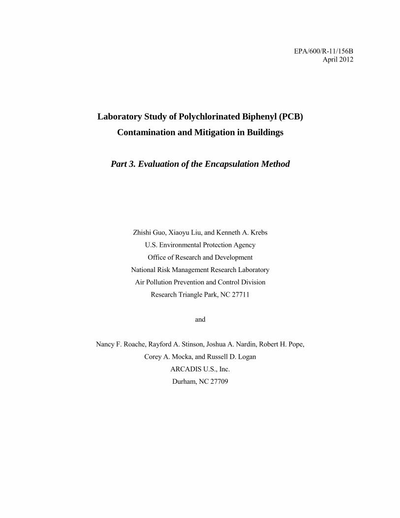
Sink tests were conducted in small environmental chambers, as illustrated in Figure E.1. The source chamber provided gas-phase PCBs emitted from building caulk. Coating materials (encapsulants) were applied to stainless steel disks that measured 1.27 cm in diameter and the disks were cured in a fume hood. For each encapsulant, 20 disks were placed in the test chamber (Figure E.2). The tests were conducted at 23 ˚C, 46% relative humidity, and one air change per hour. During the tests, four of the 20 disks were removed from the source chamber at a given time, followed by subsequent removals of four disks at four different times. This procedure was followed for all encapsulants tested, and the PCB concentrations associated with the encapsulated disks were determined by extraction with hexane and analysis by gas chromatography/mass spectrometry (GC/MS).

Source Chamber Test Chamber

Sliced Caulk

PUF PUF

Sink Materials Clean

Air

Fan Fan

iv

Figure E.1. Schematic of the two-chamber system for sink tests

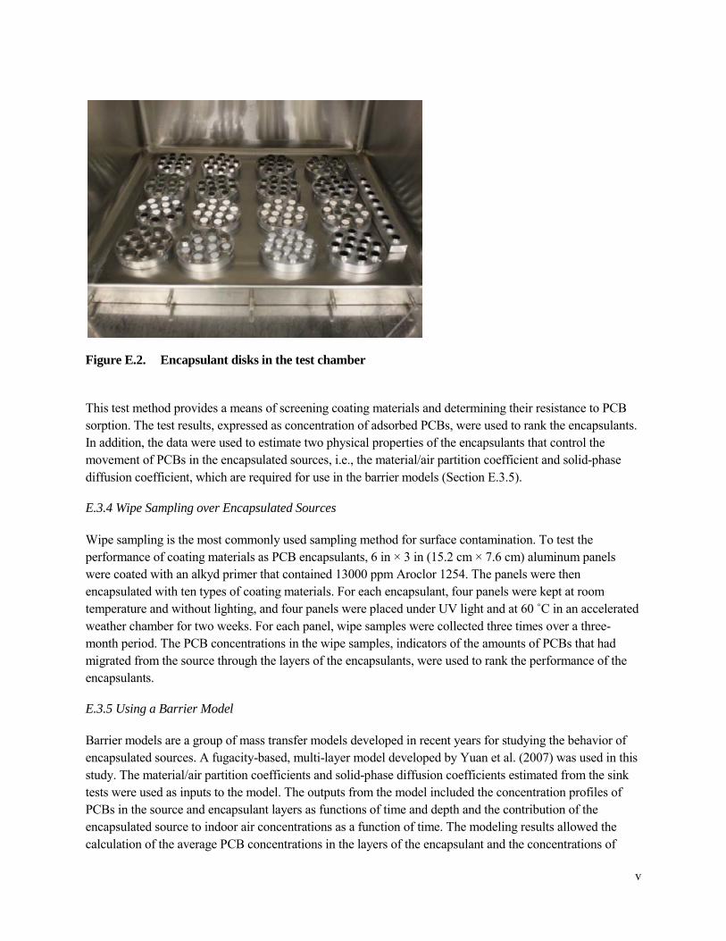
Figure E.2. Encapsulant disks in the test chamber

This test method provides a means of screening coating materials and determining their resistance to PCB sorption. The test results, expressed as concentration of adsorbed PCBs, were used to rank the encapsulants. In addition, the data were used to estimate two physical properties of the encapsulants that control the movement of PCBs in the encapsulated sources, i.e., the material/air partition coefficient and solid-phase diffusion coefficient, which are required for use in the barrier models (Section E.3.5).

E.3.4 Wipe Sampling over Encapsulated Sources

Wipe sampling is the most commonly used sampling method for surface contamination. To test the performance of coating materials as PCB encapsulants, 6 in × 3 in (15.2 cm × 7.6 cm) aluminum panels were coated with an alkyd primer that contained 13000 ppm Aroclor 1254. The panels were then encapsulated with ten types of coating materials. For each encapsulant, four panels were kept at room temperature and without lighting, and four panels were placed under UV light and at 60 ˚C in an accelerated weather chamber for two weeks. For each panel, wipe samples were collected three times over a three-month period. The PCB concentrations in the wipe samples, indicators of the amounts of PCBs that had migrated from the source through the layers of the encapsulants, were used to rank the performance of the encapsulants.

E.3.5 Using a Barrier Model

Barrier models are a group of mass transfer models developed in recent years for studying the behavior of encapsulated sources. A fugacity-based, multi-layer model developed by Yuan et al. (2007) was used in this study. The material/air partition coefficients and solid-phase diffusion coefficients estimated from the sink tests were used as inputs to the model. The outputs from the model included the concentration profiles of PCBs in the source and encapsulant layers as functions of time and depth and the contribution of the encapsulated source to indoor air concentrations as a function of time. The modeling results allowed the calculation of the average PCB concentrations in the layers of the encapsulant and the concentrations of

v

PCB at the exposed surfaces of the encapsulant at different times. These concentrations were then used to rank the performance of the encapsulants.

E.4 Findings

E.4.1 Sink Tests

The experimentally-determined sorption concentrations for a water-borne acrylic coating material and an epoxy coating material are shown in Figures E.3 and E.4, respectively. The sorption concentrations differed by roughly a factor of 20 between the two coating materials, indicating that the epoxy coating is more resistant to the sorption of PCBs than the water-borne acrylic coating.

10

So

rpti

on

Co

nce

ntr

ati

on

(μ

g/c

m2)

1

0.1

0.01

0 100 200 300 400 500

PCB-17

PCB-52

PCB-66

PCB-101

PCB-105

PCB-110

PCB-118

PCB-154

0.001

Elapsed Time (h)Title

Figure E.3. Experimentally determined sorption concentrations of PCB congeners for a waterborne acrylic coating

vi

So

rpti

on

Co

nce

ntr

ati

on

(μ

g/c

m2)

10

1

PCB-52

PCB-66

PCB-101

0.1 PCB-105

PCB-110

0.01 PCB-118

PCB-154

0.001

0 100 200 300

Elpased Time (h)

400 500

Figure E.4. Experimentally determined sorption concentrations of PCB congeners for an epoxy coating

(The concentrations of congener #17 were below the practical quantification limit)

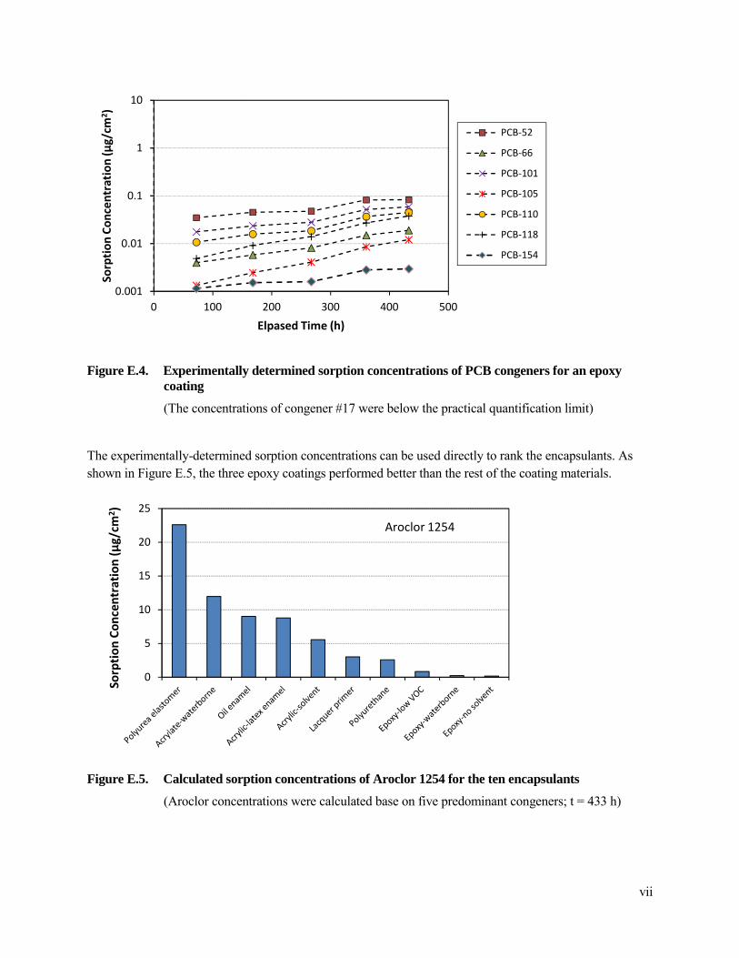
The experimentally-determined sorption concentrations can be used directly to rank the encapsulants. As shown in Figure E.5, the three epoxy coatings performed better than the rest of the coating materials.

So

rpti

on

Co

nce

ntr

ati

on

(μ

g/c

m2) 25

20

15

10

5

0

Aroclor 1254

Figure E.5. Calculated sorption concentrations of Aroclor 1254 for the ten encapsulants

(Aroclor concentrations were calculated base on five predominant congeners; t = 433 h)

vii

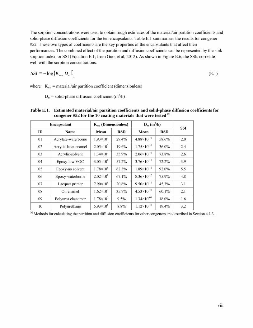
The sorption concentrations were used to obtain rough estimates of the material/air partition coefficients and solid-phase diffusion coefficients for the ten encapsulants. Table E.1 summarizes the results for congener #52. These two types of coefficients are the key properties of the encapsulants that affect their performances. The combined effect of the partition and diffusion coefficients can be represented by the sink sorption index, or SSI (Equation E.1; from Guo, et al, 2012). As shown in Figure E.6, the SSIs correlate well with the sorption concentrations.

SSI = − log (Kma Dm ) (E.1) ,

where Kma = material/air partition coefficient (dimensionless)

Dm = solid-phase diffusion coefficient (m2/h)

Table E.1. Estimated material/air partition coefficients and solid-phase diffusion coefficients for congener #52 for the 10 coating materials that were tested [a]

Encapsulant Kma (Dimensionless) Dm (m2/h)

SSI ID Name Mean RSD Mean RSD

01 Acrylate-waterborne 1.93×107 29.4% 4.88×10-10 58.6% 2.0

02 Acrylic-latex enamel 2.05×107 19.6% 1.75×10-10 36.0% 2.4

03 Acrylic-solvent 1.34×107 35.9% 2.06×10-10 73.8% 2.6

04 Epoxy-low VOC 3.05×106 57.2% 3.76×10-11 72.2% 3.9

05 Epoxy-no solvent 1.78×106 62.3% 1.89×10-12 92.0% 5.5

06 Epoxy-waterborne 2.02×106 67.1% 8.36×10-12 75.9% 4.8

07 Lacquer primer 7.90×106 20.6% 9.50×10-11 45.3% 3.1

08 Oil enamel 1.62×107 35.7% 4.53×10-10 60.1% 2.1

09 Polyurea elastomer 1.78×107 9.5% 1.34×10-09 18.0% 1.6

10 Polyurethane 5.93×106 8.8% 1.12×10-10 19.4% 3.2 [a] Methods for calculating the partition and diffusion coefficients for other congeners are described in Section 4.1.3.

viii

So

rpti

on

Co

nce

ntr

ati

on

(μ

g/c

m2

) 10

1

0.1

0.01

0.001

1.00 2.00 3.00 4.00 5.00 6.00

SSI

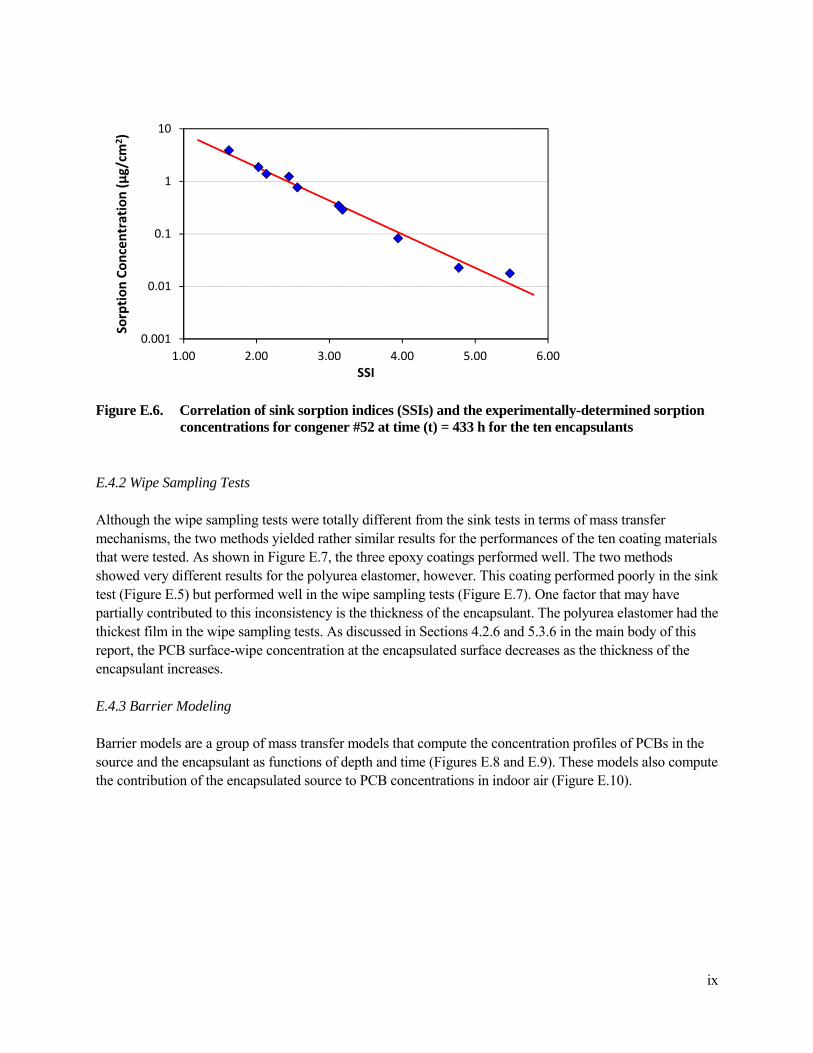
Figure E.6. Correlation of sink sorption indices (SSIs) and the experimentally-determined sorption concentrations for congener #52 at time (t) = 433 h for the ten encapsulants

E.4.2 Wipe Sampling Tests

Although the wipe sampling tests were totally different from the sink tests in terms of mass transfer mechanisms, the two methods yielded rather similar results for the performances of the ten coating materials that were tested. As shown in Figure E.7, the three epoxy coatings performed well. The two methods showed very different results for the polyurea elastomer, however. This coating performed poorly in the sink test (Figure E.5) but performed well in the wipe sampling tests (Figure E.7). One factor that may have partially contributed to this inconsistency is the thickness of the encapsulant. The polyurea elastomer had the thickest film in the wipe sampling tests. As discussed in Sections 4.2.6 and 5.3.6 in the main body of this report, the PCB surface-wipe concentration at the encapsulated surface decreases as the thickness of the encapsulant increases.

E.4.3 Barrier Modeling

Barrier models are a group of mass transfer models that compute the concentration profiles of PCBs in the source and the encapsulant as functions of depth and time (Figures E.8 and E.9). These models also compute the contribution of the encapsulated source to PCB concentrations in indoor air (Figure E.10).

ix

0

200

400

600

800 A

rocl

or

12

54

(μ

g/1

00

cm

2 )

t = 167 hours

120

100

Concrete / Lacquer-primer

0 1 2 3 4 5

C1(

x) (

μg

/g) 80

60

40

20

0

1 day

10 days

100 days

1000 days

5000 days

x (mm)

Figure E.7. Concentration of Aroclor 1254 in the first round wipe samples taken over encapsulated PCB panels that underwent aging at room temperature

(The results are semi-quantitative, and the error bar is ±1 SD)

Figure E.8. Concentration profiles for congener #110 in the source (concrete) encapsulated with a lacquer primer [C1(x)]

(Source/encapsulant interface is at x = 5 mm; the initial source concentration is 100 µg/g.)

x

0

20

40

60

80 C

2 (x)

(u

g/g

)

1 day

10 days

100 days

1000 days

5000 days

Concrete / Lacquer-primer

0.00 0.02 0.04 0.06 0.08 0.10

x (mm)

Figure E.9. Concentration profiles for congener #110 in the layer of encapsulant (lacquer primer) as a function of depth [C2(x)]

(The interface between the source and the encapsulant is at x = 0 mm; the exposed surface is at x = 0.1 mm; the initial concentration in the source (C01) is 100 µg/g)

1.2

Air

co

nce

ntr

ati

on

(μ

g/m

3)

0.9

0.6

0.3

0.0

Lacquer primer

Epoxy-waterborne

0 1000 2000 3000 4000 5000

Elapsed Time (days)

Figure E.10. Concentration of congener #110 in room air due to emissions from the encapsulated sources as function of time

(The initial concentration in the source is 100 µg/g; the source area is 10 m2)

xi

The modeling results showed that, for a given PCB source and encapsulant pair, a linear correlation exists between the initial concentration in the source and the average concentration in the encapsulant (Figure E.11), indicating the limitations of the encapsulation method: (1) Encapsulation is not effective for reducing surface concentrations and indoor air levels for sources that have high PCB content, and (2) The upper limit of the PCB content in the source for which encapsulation would be effective is determined by the performance of the encapsulant and mitigation goal. The more stringent the goal is, the lower the concentration in the source is allowed. More details are provided in Section 6.1.

400

Lacquer primer

Epoxy-waterborne 300

200

100

t = 100 days 0

0 200 400 600 800 1000 1200

Initial Concentration in Source (μg/g)

Figure E.11. Average concentration in the layer of encapsulant (average C2) as a function of initial concentration in the source (t = 100 days)

Using the partition coefficients and diffusion coefficients obtained from the sink tests, the relative performance of the ten encapsulants can be ranked. As an example, Figure E.12 compares the predicted PCB concentrations at the exposed surface when a source is encapsulated with different encapsulants.

Av

era

ge

C2

(μ

g/g

)

xii

C

2 (

Su

rfa

ce)

(μg

/g)

25

20

15

10

5

0

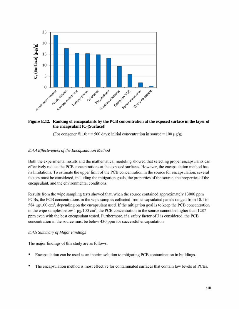
Figure E.12. Ranking of encapsulants by the PCB concentration at the exposed surface in the layer of the encapsulant [C2(Surface)]

(For congener #110; t = 500 days; initial concentration in source = 100 µg/g)

E.4.4 Effectiveness of the Encapsulation Method

Both the experimental results and the mathematical modeling showed that selecting proper encapsulants can effectively reduce the PCB concentrations at the exposed surfaces. However, the encapsulation method has its limitations. To estimate the upper limit of the PCB concentration in the source for encapsulation, several factors must be considered, including the mitigation goals, the properties of the source, the properties of the encapsulant, and the environmental conditions.

Results from the wipe sampling tests showed that, when the source contained approximately 13000 ppm PCBs, the PCB concentrations in the wipe samples collected from encapsulated panels ranged from 10.1 to 584 µg/100 cm2, depending on the encapsulant used. If the mitigation goal is to keep the PCB concentration in the wipe samples below 1 µg/100 cm2, the PCB concentration in the source cannot be higher than 1287 ppm even with the best encapsulant tested. Furthermore, if a safety factor of 3 is considered, the PCB concentration in the source must be below 430 ppm for successful encapsulation.

E.4.5 Summary of Major Findings

The major findings of this study are as follows:

• Encapsulation can be used as an interim solution to mitigating PCB contamination in buildings.

• The encapsulation method is most effective for contaminated surfaces that contain low levels of PCBs.

xiii

• As demonstrated in Part 2 of this report series, the secondary sources may become emitting sources of PCBs after the primary sources are removed. Because of their large quantities, mitigating secondary sources is difficult and costly. The encapsulation method has the potential to substantially reduce the cost by not having to remove the contaminated materials from the building.

• Selecting high-performance coating materials is a key to effective encapsulation. Multiple layers of coatings enhance the performance of the encapsulation. Post-encapsulation inspection and monitoring is essential for successful encapsulation.

• For effective encapsulation, the maximum allowable concentration of PCBs in the source is estimated to be 430 ppm, assuming (1) the maximum allowable PCB concentration in the wipe sample is 1 µg/100 cm2, (2) the most effective encapsulant we tested is used, and (3) the safety factor is 3.

• Encapsulating primary sources, such as old caulk, that contain high concentrations of PCBs can be beneficial, but may not be sufficient to reduce the surface and air concentrations to desirable levels.

• The experimental methods developed in this report can be used to screen more coating materials.

E.5 Study Limitations

This study was limited to laboratory testing with a limited scope. Only ten coating materials were tested. There are many coating materials that can potentially be used as PCB encapsulants. The test results of this study may not be applicable to the similar products that were not tested even within the same class of coatings.

This study was narrowly focused on the effectiveness and limitations of the encapsulation method, the performances of a limited number of encapsulants, and the factors that may affect the performance of encapsulation. It is not a comprehensive evaluation of the encapsulation method, which involves multiple steps.

This study investigated liquid encapsulants only. Encapsulation by using solid materials was not studied. In practice, multiple coating materials are often used (such as using a primer before applying the encapsulant), which were not tested in this study.

Part of the wipe samples were analyzed by a commercial analytical laboratory. The results did not meet all the data quality criteria to qualify as quantitative data. The accuracy and precision of the data were in the range of 25% to 50%. Thus, the data generated by the commercial laboratory should be considered semi-quantitative.

The material/air partition coefficients and solid-phase diffusion coefficients reported are rough estimates. For more accurate measurements, the two parameters must be determined separately.

The correlation of the PCB concentration in the surface material with the concentration in the wipe samples is poorly understood. This data gap makes it difficult to link the wipe sampling results to the barrier models.

xiv

TABLE OF CONTENTS

Executive Summary..........................................................................................................................................iii

E.1 Background...............................................................................................................................................iii

E.2 Objective...................................................................................................................................................iii

E.3 Methods ....................................................................................................................................................iv E.3.1 Technical Approach.....................................................................................................................iv E.3.2 Test Materials...............................................................................................................................iv E.3.3 Sink Tests in Small Chambers.....................................................................................................iv E.3.4 Wipe Sampling over Encapsulated Sources.................................................................................v E.3.5 Using a Barrier Model ..................................................................................................................v

E.4 Findings ....................................................................................................................................................vi E.4.1 Sink Tests.....................................................................................................................................vi E.4.2 Wipe Sampling Tests...................................................................................................................ix E.4.3 Barrier Modeling..........................................................................................................................ix E.4.4 Effectiveness of the Encapsulation Method..............................................................................xiii E.4.5 Summary of Major Findings .....................................................................................................xiii

E.5 Study Limitations ...................................................................................................................................xiv

List of Tables ................................................................................................................................................ xviii

List of Figures...................................................................................................................................................xx

Acronyms and Abbreviations......................................................................................................................xxiv

1. Introduction...................................................................................................................................................1

1.1 Background.............................................................................................................................................1

1.2 Goals and Objectives..............................................................................................................................2

1.3 Technical Approach ...............................................................................................................................2

1.4 About This Report ..................................................................................................................................3

2. Experimental Methods.................................................................................................................................4

2.1 Test Specimens.......................................................................................................................................4

2.2 Sink Tests in 53-L Environmental Chambers........................................................................................4 2.2.1 Test Facility...............................................................................................................................4 2.2.2 Preparation of the Coating Materials .......................................................................................7 2.2.3 Test Procedure ..........................................................................................................................9

2.3 Wipe Sampling over Encapsulated Sources ..........................................................................................9 2.3.1 Preparation of Source Panels....................................................................................................9

xv

2.3.2 Application of Encapsulant ....................................................................................................10 2.3.3 Aging at Room Temperature..................................................................................................11 2.3.4 Accelerated Aging ..................................................................................................................12

2.4 Sampling and Analysis.........................................................................................................................13 2.4.1 Internal Standards and Recovery Check Standards ...............................................................13 2.4.2 Air Sampling...........................................................................................................................13 2.4.3 Extraction of Encapsulant-Coated Disks ...............................................................................13 2.4.4 Wipe Sampling .......................................................................................................................14 2.4.5 Sample Analysis .....................................................................................................................15

3. Quality Assurance and Quality Control ..................................................................................................16

3.1 QA/QC for the In-house Analytical Laboratory..................................................................................16 3.1.1 GC/MS Instrument Calibration ..............................................................................................16 3.1.2 Detection Limits .....................................................................................................................17 3.1.3 Environmental Parameters......................................................................................................18 3.1.4 Quality Control Samples ........................................................................................................19 3.1.5 Recovery Check Standards.....................................................................................................22

3.2 QA/QC for Using a Commercial Analytical Laboratory ....................................................................22 3.2.1 QA/QC Procedure...................................................................................................................23 3.2.2 Data Quality Indicators (DQIs) ..............................................................................................23 3.2.3 Data Quality Evaluation .........................................................................................................23 3.2.4 Conclusion Related to Data Quality Review .........................................................................25

4. Experimental Results..................................................................................................................................26

4.1 Sink Tests..............................................................................................................................................26 4.1.1 Test Conditions .......................................................................................................................26 4.1.2 Experimentally Determined Sorption Concentrations...........................................................28 4.1.3 Estimation of the Partition and Diffusion Coefficients .........................................................32

4.2 Wipe Sampling over Encapsulated Sources ........................................................................................35 4.2.1 PCB Concentrations in the Source.........................................................................................35 4.2.2 Thicknesses of the Dry Films of the Encapsulants ................................................................35 4.2.3 Wipe Samples for Not-encapsulated Sources That Had Undergone Aging at Room

Temperature ............................................................................................................................36 4.2.4 Encapsulated Sources That Had Undergone Ageing at Room Temperature........................36 4.2.5 Encapsulated Sources That Had Undergone Accelerated Aging ..........................................40 4.2.6 Additional Wipe Sampling Tests ...........................................................................................43

5. Mathematical Modeling .............................................................................................................................48

5.1 Model Description................................................................................................................................48

xvi

5.1.1 Available Barrier Models .......................................................................................................48 5.1.2 The Concept of Fugacity ........................................................................................................48 5.1.3 The Fugacity-Based Barrier Model........................................................................................49

5.2 Input Parameters...................................................................................................................................51 5.2.1 Parameters Required by the Model ........................................................................................51 5.2.2 Parameter Values for the “Base-case” Scenario ....................................................................51

5.3 General Behavior of Encapsulated Sources.........................................................................................52 5.3.1 Concentration Profiles in the Source......................................................................................52 5.3.2 Concentration Profiles in the Encapsulant Layer...................................................................54 5.3.3 Average Concentration in the Encapsulant Layer .................................................................55 5.3.4 Concentration at the Exposed Surface ...................................................................................56 5.3.5 Contribution to PCB Concentrations in Room Air................................................................56 5.3.6 Effect of the Thickness of the Encapsulant............................................................................56 5.3.7 Effect of Contaminant Concentration in the Source..............................................................61

5.4 Ranking the Encapsulants ....................................................................................................................64 5.4.1 Performance Indicators...........................................................................................................64 5.4.2 Input Parameters for the Barrier Model .................................................................................64 5.4.3 Ranking the Encapsulants Based on Absolute Concentrations .............................................65 5.4.4 Ranking the Encapsulants Based on Percent Reduction of Concentrations .........................67

5.5 Limitations of Mathematical Modeling...............................................................................................69

6. Discussion.....................................................................................................................................................70

6.1 Effectiveness and Limitations of the Encapsulation Method..............................................................70

6.2 Selection of Encapsulants.....................................................................................................................71

6.3 Potential Effect of the Weathering of Encapsulants on their Encapsulating Ability..........................72

6.4 Encapsulating Encapsulated Sources...................................................................................................73

6.5 Effectiveness of Encapsulating Sources with High PCB Content ......................................................73

6.6 Relationship between the Sink Tests and the Wipe Sampling Tests ..................................................73

6.7 Study Limitations .................................................................................................................................74

7. Conclusions..................................................................................................................................................75

8. Recommendations.......................................................................................................................................77

Acknowledgments ............................................................................................................................................78

References .........................................................................................................................................................79

Appendix A. Evaluation of the Wipe Sampling Method.............................................................................82

Appendix B. Resistance of the Encapsulants to Abrasion ..........................................................................84

xvii

List of Tables

Table E.1. Estimated material/air partition coefficients and solid-phase diffusion coefficients for congener #52 for the 10 coating materials that were tested viii

Table 2.1. Coating materials tested (product names, binder types, recommended uses, and recommended application methods) 5

Table 2.2. Coating materials tested (principal solvents, VOC content, solid content, and recommended application rates) 6

Table 2.3. Application methods and number of coats for the encapsulated panels 11 Table 3.1. GC/MS calibration for PCB congeners from Aroclor 1254 17 Table 3.2. IAP results for each calibration related to this study 18 Table 3.3. Instrument detection limits (IDLs) for PCB congeners on GC/MS (ng/mL) 18 Table 3.4. Background concentrations of PCBs (µg/m3) in the chamber for the sink test 19 Table 3.5. Concentration of PCBs in the field blank samples (ng) 20 Table 3.6. Concentration of PCBs in the method blank samples (µg/cm2 wipe sample) for the

accelerated weathering process 21 Table 3.7. Concentration of PCBs in the method blank samples (µg/cm2 wipe sample) for panels

in the storage cabinet 21 Table 3.8. Average recoveries of DCCs for the tests of the encapsulants 22 Table 3.9. Criteria for determining the usability of data reported by the commercial laboratory 23 Table 3.10. QC samples for evaluating the accuracy of the analytical results reported by the

commercial laboratory 24 Table 3.11. QC samples for evaluating the precision of the analytical results reported by the

commercial laboratory 24 Table 3.12. QC samples for evaluating the potential contamination in the laboratory and during

transportation of samples 24 Table 3.13. Recovery of the recovery check standards (RCSs) for all wipe samples analyzed by the

commercial laboratory 25 Table 4.1. Conditions of the test chamber 26 Table 4.2. Thicknesses of the dry films of the encapsulants used for the sink test 26 Table 4.3. Estimated partition coefficient (Kma), diffusion coefficient (Dm) for the reference

congener (#52) and index α in Equation 4.2 34 Table 4.4. Concentrations of target congeners in three batches of dry primer 35 Table 4.5. Thickness of dry films of the encapsulants for the wipe sampling tests 36 Table 4.6. Concentrations of Aroclor 1254 in wipe samples taken from not-encapsulated source

panels 36 Table 4.7 Percent reduction of PCB concentrations in wipe samples for encapsulated PCB

sources 40

xviii

Table 4.8. PCB concentrations in cured substrates 46 Table 5.1. Input parameters for the fugacity model 51 Table 5.2. Base-case values for the simulations 52 Table 5.3. Partition coefficients (Kma) and diffusion coefficients (Dm) for congener #110 for the

source and encapsulants 52 Table 5.4. Material/air partition coefficients (Kma) and solid-phase diffusion coefficients (Dm) for

congener #110 used for ranking the encapsulants 64 Table 5.5. Ranking the encapsulants by percent reduction of the average concentration in the top

0.1 mm of the layer, i.e., the thickness of the encapsulant 68 Table 5.6. Ranking the encapsulants by percent reduction of the concentration at the exposed

surface 68 Table 5.7. Ranking the encapsulants by percent reduction of the concentration in room air 69 Table 6.1. Calculated maximum allowable concentrations in the source for effective encapsulation

with two mitigation goals based on the PCB concentration in wipe samples (Wmax) 72

xix

List of Figures

Figure E.1. Schematic of the two-chamber system for sink tests v Figure E.2. Encapsulant disks in the test chamber v Figure E.3. Experimentally determined sorption concentrations of PCB congeners for a waterborne

acrylic coating vi Figure E.4. Experimentally determined sorption concentrations of PCB congeners for an epoxy

coating vii Figure E.5. Calculated sorption concentrations of Aroclor 1254 for the ten encapsulants vii Figure E.6. Correlation of sink sorption indices (SSIs) and the experimentally-determined sorption

concentrations for congener #52 at time (t) = 433 h for the ten encapsulants ix Figure E.7. Concentration of Aroclor 1254 in the first round wipe samples taken over encapsulated

PCB panels that underwent aging at room temperature x Figure E.8. Concentration profiles for congener #110 in the source encapsulated with a lacquer

primer [C1(x)] x Figure E.9. Concentration profiles for congener #110 in the layer of encapsulant (lacquer primer)

as a function of depth [C2(x)] xi Figure E.10. Concentration of congener #110 in room air due to emissions from the encapsulated

source as function of time xi Figure E.11. Average concentration in the layer of encapsulant (average C2) as a function of initial

concentration in the source (t = 100 days) xii Figure E.12. Ranking of encapsulants by the PCB concentration at the exposed surface in the layer

of the encapsulant [C2(Surface)] xiii Figure 2.1. Schematic of the two-chamber system for sink tests, showing the air flows and

sampling locations (PUF samples) 7 Figure 2.2. Chamber system for sink tests: source chamber (top) and test chamber (bottom) 7 Figure 2.3. Painted stainless steel panel after the disks were punched out 8 Figure 2.4. Sample stage with aluminum pin mounts 8 Figure 2.5. Sample stages in the test chamber 9 Figure 2.6. Taped panel (left); panel after primer was applied (right) 10 Figure 2.7. Re-taped panel with dried primer (left); panel after application of the encapsulant

(right) 10 Figure 2.8. Plastic cabinets (left); panels inside a plastic cabinet (right) 11 Figure 2.9. Wooden cabinets that housed the plastic cabinets 12 Figure 2.10. QUV Accelerated Weathering Tester: exterior (left); UV lamps (right) 12 Figure 2.11. Wipe sampling process: wipe on panel (left); wipe covered with foil (center); roller

method (right) 14 Figure 4.1. Concentrations of the target congeners in the air of the test chamber (normal scale) 27

xx

Figure 4.2. Concentrations of the target congeners in the air of the test chamber (semi-log scale) 27 Figure 4.3. Experimentally-determined sorption concentrations as a function of time for the

Acrylate-waterborne coating material (top: normal scale; bottom: semi-log scale). 29 Figure 4.4. Experimentally-determined sorption concentrations as a function of time for the

Epoxy-low VOC coating material (top: normal scale; bottom: semi-log scale). 30 Figure 4.5. Experimentally-determined sorption concentrations for congener #52 for the ten

encapsulants (t = 433 h) 31 Figure 4.6. Experimentally-determined sorption concentrations for congener #110 for the ten

encapsulants (t = 433 h) 31 Figure 4.7. Calculated sorption concentrations for Aroclor 1254 for the ten encapsulants (t = 433

h) 32 Figure 4.8. Goodness-of-fit for estimating the partition and diffusion coefficients for the Acrylic-

solvent coating material 33 Figure 4.9. Concentration of Aroclor 1254 in the first-round wipe samples taken over encapsulated

PCB panels that had undergone aging at room temperature (error bar = ±1 SD) 37 Figure 4.10. Concentrations of Aroclor 1254 in the second-round wipe samples taken over

encapsulated PCB panels that had undergone aging room temperature (error bar = ±1 SD) 38

Figure 4.11. Concentrations of Aroclor 1254 in the third-round wipe samples taken over encapsulated PCB panels that had undergone aging at room temperature (error bar = ±1 SD) 38

Figure 4.12. Concentrations of Aroclor 1254 for the sum of three rounds of wipe samples taken over encapsulated PCB panels that had undergone aging at room temperature 39

Figure 4.13. Concentration of Aroclor 1254 in the first-round wipe samples taken over encapsulated PCB panels that had undergone accelerated aging (error bar = ±1 SD) 41

Figure 4.14. Concentration of Aroclor 1254 in the second-round wipe samples taken over encapsulated PCB panels that had undergone accelerated aging (error bar = ±1 SD) 41

Figure 4.15. Concentration of Aroclor 1254 in the third-round wipe samples taken over encapsulated PCB panels that had undergone accelerated aging (error bar = ±1 SD) 42

Figure 4.16. Concentrations of Aroclor 1254 for the sum of three rounds of wipe samples taken over encapsulated PCB panels that had undergone accelerated aging 42

Figure 4.17. Comparison of wipe sampling results (the sum of three wipes) for the two aging methods 43

Figure 4.18. Concentrations of target congeners in wipe samples taken at 167 elapsed hours 44 Figure 4.19. Concentrations of target congeners in wipe samples taken at 692 elapsed hours 44 Figure 4.20. Concentrations of target congeners in wipe samples taken at 1245 elapsed hours. 45 Figure 4.21. Concentrations of Aroclor 1254 in three wipe samples taken at 167, 692, and 1245

elapsed hours 45 Figure 4.22. Effect of source substrate on PCB concentrations in wipe samples ― the sources

(primer and caulk) were encapsulated with the Lacquer-primer (error bar = ±1 SD) 47

xxi

Figure 4.23. Effect of source substrate on PCB concentrations in wipe samples ― the sources (primer and caulk) were encapsulated with Polyurethane (error bar = ±1 SD) 47

Figure 5.1. Schematic representation of the double-layer model (Yuan et al., 2007) 49 Figure 5.2. Concentration profiles for congener #110 in the source encapsulated with a Lacquer-

primer [C1(x)]. 53 Figure 5.3. Concentration profiles for congener #110 in the source encapsulated with a waterborne

epoxy coating [C1(x)] 53 Figure 5.4. Concentration profiles for congener #110 in the encapsulant layer (Lacquer primer) as

a function of depth 54 Figure 5.5. Concentration profiles for congener #110 in the encapsulant layer (Epoxy-waterborne)

as a function of depth 55 Figure 5.6. The average concentration of congener #110 in the encapsulant layer (C2) as a function

of time 56 Figure 5.7. Concentration of congener #110 at the exposed surface of the encapsulant [C2(x=L2)]

as a function of time 57 Figure 5.8. Concentration of congener #110 in room air due to emissions from the encapsulated

source as a function of time 57 Figure 5.9. Effect of the thickness of the encapsulant on the average concentration of congener

#110 in the encapsulant layer (average C2) ― Case 1: Lacquer primer 58 Figure 5.10. Effect of the thickness of the encapsulant on the average concentration of congener

#110 in the encapsulant layer (average C2) ― Case 2: Epoxy-waterborne 58 Figure 5.11. Effect of the thickness of the encapsulant on the concentration of congener #110 at the

exposed surface of the encapsulant [C2(x=L2)] ― Case 1: Lacquer-primer 59 Figure 5.12. Effect of the thickness of the encapsulant on the concentration of congener #110 at the

exposed surface of the encapsulant [C2(x=L2)] ― Case 2: Epoxy-waterborne 59 Figure 5.13. Effect of encapsulant thickness on the concentration of congener #110 in room air due

to emissions from the encapsulated source ― Case 1: Lacquer-primer 60 Figure 5.14. Effect of encapsulant thickness on the concentration of congener #110 in room air due

to emissions from the encapsulated source ― Case 2: Epoxy-waterborne 60 Figure 5.15. Average concentration of congener #110 in the encapsulant layer (average C2) as a

function of initial concentration in the source (t = 100 days) 61 Figure 5.16. Average concentration of congener #110 in the encapsulant layer (average C2) as a

function of initial concentration in the source (t = 1000 days) 61 Figure 5.17. Concentration of congener #110 at the exposed surface of the encapsulant layer [C2(x =

L2)] as a function of initial concentration in the source (t = 100 days) 62 Figure 5.18. Concentration of congener #110 at the exposed surface of the encapsulant layer [C2(x =

L2)] as a function of initial concentration in the source (t = 1000 days) 62 Figure 5.19. Contribution of the encapsulated source to the concentration of congener #110 in room

air as a function of initial concentration in the source (t = 100 days) 63 Figure 5.20. Contribution of the encapsulated source to the concentration of congener #110 in room

air as a function of initial concentration in the source (t = 1000 days) 63

xxii

Figure 5.21. Ranking of encapsulants by the average concentration in the encapsulant layer (Average C2) 65

Figure 5.22. Ranking of encapsulants by the concentration at the exposed surface of the encapsulant layer [C2 (x=L2)] 66

Figure 5.23. Ranking of encapsulants by the air concentration due to emissions from the encapsulated source 66

Figure 5.24. Concentration profiles for congener #110 in not-encapsulated concrete at t = 500 days 67

xxiii

Acronyms and Abbreviations

DAS Data acquisition system

DCC Daily calibration check

DQI Data quality indicator

GC/ECD Gas chromatography/electron capture detector

GC/MS Gas chromatography/mass spectrometry

IAP Internal audit program

IDL Instrument detection limit

LC Laboratory control

ND Not detected

NELAP National Environmental Laboratory Approval Program

NERL National Exposure Research Laboratory

ORD Office of Research and Development

PCB Polychlorinated biphenyl

PQL Practical quantification limit

PUF Polyurethane foam

QA Quality assurance

QAPP Quality Assurance Project Plan

QC Quality control

RCS Recovery check standard

RH Relative humidity

RRF Relative response factor

RSD Relative standard deviation

SD Standard deviation

TCMX Tetrachloro-m-xylene or tetrachlorometaxylene

UV Ultraviolet

VOC Volatile organic compound

xxiv

1. Introduction

1.1 Background

Creating a barrier between the source of contaminants and the surrounding environment is one of the common abatement techniques for contamination in structures and buildings (Esposito et al., 1987). The encapsulating barriers may take different forms such as painting and coating, plaster, concrete casts and walls. Painting and coating techniques are the most common forms used inside buildings. Encapsulation has been used successfully for decontaminating asbestos (Brown, 1990; Brown and Angelopoulos, 1991; ASTM, 2010a), lead paint (ASTM, 2004a, 2004b, and 2011), and methamphetamine (Martyny, 2008) in buildings.

Encapsulating structures and buildings contaminated with polychlorinated biphenyls (PCBs) began in the early 1970s (Willett, 1972, 1973, 1974, 1976) and has been used since then (Mitchell and Scadden, 2001; Scadden and Mitchell, 2001; Pizarro et al., 2002; EH&E, 2012). Willett (1974) tested the feasibility of twelve coating materials as PCB encapsulants for the interior of concrete silos coated with a PCB-containing material. The author found that nine of the twelve coatings reduced the concentration of PCBs in the silage compared to silage adjacent to control surfaces. Coatings carried by water or a solvent in which PCBs are not readily soluble were the most effective barriers. Coating materials with a base coat to seal the surface prior to application of the surface coating were more effective than two applications of a single formulation. Hydraulic cement with an acrylic bonder and water-carried epoxy effectively reduced residues in silage from contaminated dairy farm silos.

Mitchell and Scadden (2001) indicated that important properties to consider when choosing an encapsulant include elongation (i.e., elasticity or rigidity), dry film thickness, hardness, drying or curing time, and compatibility with existing surfaces. Epoxy-type coatings are widely used for PCB encapsulation. Epoxy coatings generally consist of a three-part epoxy-polyamide coating applied in a primer layer, clad leveler, and surface layer. Encapsulants applied to floors should include two coatings of contrasting color to indicate when resurfacing is required due to wear. Such practice is also routinely applied on exterior walls.

Scadden and Mitchell (2001) reported a case study in which the PCB-contaminated floors were cleaned by multi-step surface washing and then encapsulated with two coats of a high-solid, water-based epoxy with contrasting colors. The authors recommended that a penetrating primer be used to help seal the concrete surface before applying the epoxy. They also noted that compliance with the manufacturer’s epoxy mixing instructions is critical. Failure to follow the manufacturer’s instructions when mixing the activator compound in the epoxy can cause a reduction in epoxy strength and result in undesirable soft spots and cracking. The epoxy application also needs to be performed under optimum environmental conditions (dry with stable temperatures) to get the best results. For floors, anti-slip materials may need to be included as part of the epoxy topcoat or placed on top of the final epoxy surface to reduce the slip hazard created by the smooth epoxy finish.

Pizarro et al. (2002) investigated encapsulation via cleaning and epoxy-coating of PCB-contaminated concrete samples from industrial plants. They concluded that epoxy coatings can be an appropriate

1

encapsulation system if the surface is prepared properly and the temperature in the area is not too high. They also concluded that metal sheet barriers could be used for high-temperature applications.

A recent literature review on PCB remediation methods (EH&E, 2012) summarized the most recent developments in applying the encapsulation method to buildings contaminated with PCBs. There are commercially available coating materials that are designed specifically for encapsulating PCBs (TWO Teknik, 2011; Robnor Resins, undated; MIC, undated).

Despite the long history of encapsulating PCBs and different levels of success reported by researchers, a number of questions regarding this mitigation method remain, including:

• To what extent can encapsulants provide protection from PCB contamination in buildings?

• How long does the protective effect last?

• What are the key attributes of a good encapsulant for PCBs?

• What are the key factors that affect the performance of the encapsulants?

• What are the limitations of the encapsulation method?

This study answers some of these questions by using a combination of laboratory testing and mathematical modeling. The results should be useful to mitigation engineers, building owners and managers, decision-makers, researchers, and the general public.

1.2 Goals and Objectives

In this study, we sought to develop a basic understanding of the encapsulation method for PCB-contaminated surface materials and the behavior of encapsulated sources. The objectives were to (1) select or develop experimental methods to evaluate the abilities of selected coating materials to encapsulate PCBs, (2) identify useful tools for studying the behavior of encapsulated sources and predicting the performance of PCB encapsulants, (3) determine the factors that affect the performance of the encapsulants, and (4) evaluate the effectiveness and limitations of the encapsulation method for PCB sources in buildings.

1.3 Technical Approach

A combination of laboratory testing and mathematical modeling was used to evaluate the encapsulation method. The approach involved the use of three interrelated components, i.e., sink tests, wipe sampling tests, and mathematical modeling.

The sink tests compared the sorption of PCBs from air by different encapsulants. The test results, expressed as sorption concentrations, were used to rank the encapsulants based on their resistance to PCB sorption. More importantly, the test results were used to estimate the solid/air partition coefficients and the solid-phase diffusion coefficients for the encapsulants, two key parameters that affect the performance of the encapsulants. An encapsulant that has smaller partition coefficient and diffusion coefficient has greater

2

resistance to PCB sorption from the air and resistance to PCB migration from the source into the encapsulant layer. Thus, the sink tests provided a screening method for comparing encapsulants.

Wipe sampling is one of the most commonly used methods for measuring surface contamination. The PCB concentration in the wipe sample collected from the encapsulated surface is an indicator for the amount of PCBs that has migrated from the source to the encapsulant layer. Thus, for a given source, the lower the concentration in the wipe sample is, the better the encapsulant performs. In this study, encapsulated PCB sources were prepared, some of which underwent natural aging, while others were subjected to accelerated aging. Wipe samples were taken over a three-month period, and the results were used to rank the coating materials. The accelerated aging tests were conducted in order to evaluate the potential effect of deterioration of the encapsulants in their performances as PCB barriers.

Mathematical modeling is an essential tool for evaluating the performance of encapsulation. Previous researchers developed several mass transfer models, known as the barrier models, for this purpose. With the partition and diffusion coefficients obtained from the sink tests, these models can be used to study the behavior of encapsulated sources and to evaluate the relative performances of the encapsulants, at least in semi-quantitative terms.

1.4 About This Report

This is the third report in the publication series entitled Laboratory Study of Polychlorinated Biphenyl (PCB) Contamination and Mitigation in Buildings, produced by the National Risk Management Research Laboratory in EPA’s Office of Research and Development (ORD). The first report (Guo et al., 2011) was a characterization of primary sources that was focused on PCB-containing caulking materials and light ballasts. The second report (Guo et al., 2012) summarized the research results for PCB transport from primary sources to PCB sinks, including interior surface materials and settled dust. This report is focused on the evaluation of the encapsulation method for controlling the concentrations of PCBs in buildings. This study was limited to a laboratory investigation, and it complements and supplements an ongoing field study in school buildings conducted by the National Exposure Research Laboratory (NERL, 2010) in EPA ORD.

3

2. Experimental Methods

2.1 Test Specimens

Ten coating materials were selected for testing (Tables 2.1 and 2.2). The selected coating materials represented a variety of binder systems, including epoxy, acrylic, polyurethane, polyurea, alkyd, and latex systems. The criteria for selecting the test specimens were as follows:

• Coating types, such as epoxy and polyurethane coatings, that have been used as PCB encapsulants in the field (Mitchell and Scadden, 2001; EH&E, 2012).

• The coating materials must be commercially available “off-the-shelf” products.

• The coatings must be suitable for the substrates of concern.

• Some commonly-used interior-coating materials, such as latex and alkyd paints, must be included for comparison.

Although some of the coating products listed in Table 2.1 have been used as PCB encapsulants for a long time, none of them was marketed as PCB encapsulants. A silicon-based coating material is currently being sold as a PCB encapsulant (TWO Teknik, 2011). This material was not included in the study because of our inability to obtain the product in a timely fashion.

Mention of trade names in Table 2.1 is only for product identification; it is not an endorsement of the products, and it is not meant to discriminate against the products that were not tested.

2.2 Sink Tests in 53-L Environmental Chambers

2.2.1 Test Facility

The sink tests were conducted in a two-chamber system as shown in Figures 2.1 and 2.2. The system consisted of two identical 53-L stainless steel chambers, which conformed to ASTM D-5116 (ASTM, 2010b). Both chambers were housed in an incubator. The source chamber contained an open Petri dish that held 10 g of PCB-containing caulk sample to serve as a stable source of gas-phase PCBs. The caulk was an interior window sealant the authors obtained from a pre-demolition building and contained approximately 10% Aroclor 1254 (See Appendix A in Guo et al., 2012). The test encapsulant materials, made as mini-disks, were placed in the test chamber. During the test, the PCB concentrations in the outlet air of the test chamber were monitored, and the encapsulant disks were removed from the test chamber at different times to determine their content of PCB congeners. Details about this system were described by Guo et al. (2012).

4

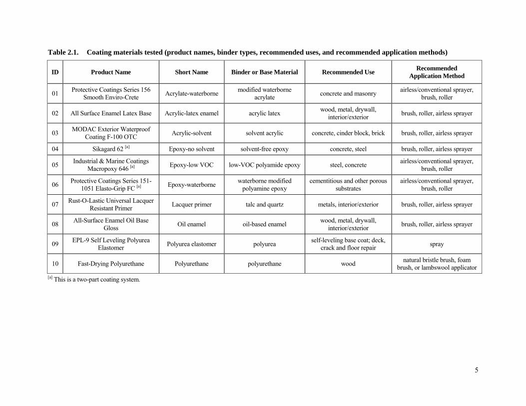
Table 2.1. Coating materials tested (product names, binder types, recommended uses, and recommended application methods)

ID Product Name Short Name Binder or Base Material Recommended Use Recommended

Application Method

01 Protective Coatings Series 156 Smooth Enviro-Crete Acrylate-waterborne modified waterborne

acrylate concrete and masonry airless/conventional sprayer, brush, roller

02 All Surface Enamel Latex Base Acrylic-latex enamel acrylic latex wood, metal, drywall, interior/exterior brush, roller, airless sprayer

03 MODAC Exterior Waterproof Coating F-100 OTC Acrylic-solvent solvent acrylic concrete, cinder block, brick brush, roller, airless sprayer

04 Sikagard 62 [a] Epoxy-no solvent solvent-free epoxy concrete, steel brush, roller, airless sprayer

05 Industrial & Marine Coatings Macropoxy 646 [a] Epoxy-low VOC low-VOC polyamide epoxy steel, concrete airless/conventional sprayer,

brush, roller

06 Protective Coatings Series 151-1051 Elasto-Grip FC [a] Epoxy-waterborne waterborne modified

polyamine epoxy cementitious and other porous

substrates airless/conventional sprayer,

brush, roller

07 Rust-O-Lastic Universal Lacquer Resistant Primer Lacquer primer talc and quartz metals, interior/exterior brush, roller, airless sprayer

08 All-Surface Enamel Oil Base Gloss Oil enamel oil-based enamel wood, metal, drywall,

interior/exterior brush, roller, airless sprayer

09 EPL-9 Self Leveling Polyurea Elastomer Polyurea elastomer polyurea self-leveling base coat; deck,

crack and floor repair spray

10 Fast-Drying Polyurethane Polyurethane polyurethane wood natural bristle brush, foam brush, or lambswool applicator

[a] This is a two-part coating system.

5

Table 2.2. Coating materials tested (principal solvents, VOC content, solid content, and recommended application rates)

ID Short Name Principle Solvent VOC Content

(g/L) Solid Content

(% w/w)

Recommended Coverage Rate

(ft2/gal) [a] Type Content (%w/w)

01 Acrylate-waterborne -- -- 49 50.9 (v/v) 100-200

02 Acrylic-latex enamel water, 2-(2-methoxyethoxy)ethanol 38, 5 132 56 350-400

03 Acrylic-solvent mineral spirits 28 445 65 690

04 Epoxy-no solvent -- 0 [b] 0 100 150-250

05 Epoxy-low VOC xylene, polyamide 17, 12 255 83 116-232

06 Epoxy-waterborne -- -- 175 17 (v/v) 180-400

07 Lacquer primer methyl isobutyl ketone, methyl propyl ketone, xylene, ethylbenzene -- 339 76 430-570

08 Oil enamel mineral oil 44 498 58 350-400

09 Polyurea elastomer -- 0 100 100

10 Polyurethane mineral spirits 48 400 -- 500 [a] To convert (ft2/gal) to (m2/L), multiply the values in the table by 0.0245. [b] According to the MSDS for this product, Part A contains unspecified amount of aromatic hydrocarbon blend and Part B contains benzyl alcohol.

6

Source Chamber Test Chamber

Sliced Caulk

PUF PUF

Sink Materials Clean

Air

Fan Fan

Figure 2.1. Schematic of the two-chamber system for sink tests, showing the air flows and sampling locations (PUF samples)

Figure 2.2. Chamber system for sink tests: source chamber (top) and test chamber (bottom)

2.2.2 Preparation of the Coating Materials

For the chamber tests, the encapsulants were applied to stainless steel disks with diameters of 0.5 inch (1.27 cm). To prepare the disks, the encapsulants were painted onto thin stainless steel panels with a paint brush, and the panels were placed in a ventilated fume hood for curing. The disks were created by using a steel arch punch (Figure 2.3). Twenty-four disks were prepared for each encapsulant, four of which were designated as background samples and placed directly into 20-mL vials for extraction and analysis. The

7

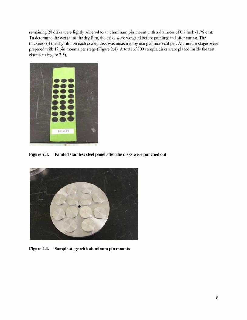
remaining 20 disks were lightly adhered to an aluminum pin mount with a diameter of 0.7 inch (1.78 cm). To determine the weight of the dry film, the disks were weighed before painting and after curing. The thickness of the dry film on each coated disk was measured by using a micro-caliper. Aluminum stages were prepared with 12 pin mounts per stage (Figure 2.4). A total of 200 sample disks were placed inside the test chamber (Figure 2.5).

Figure 2.3. Painted stainless steel panel after the disks were punched out

Figure 2.4. Sample stage with aluminum pin mounts

8

Figure 2.5. Sample stages in the test chamber

2.2.3 Test Procedure

Prior to the sink test, an air sample was collected from the exhaust flow from the test chamber by using a polyurethane foam (PUF) sampler. The exhaust flow from the source chamber was then redirected to serve as the inlet flow for the test chamber to begin the testing phase. Daily PUF samples were taken overnight on the test chamber and occasionally from the source chamber to ensure the consistency of the emissions. At an elapsed time of 72 hours, the test chamber was disconnected briefly from the source flow and opened inside a fume hood. Four disks of each type of encapsulant were removed from the chamber and placed in a 20-mL vial for extraction and analysis. The chamber was then placed back in the incubator immediately and reconnected to the flow of the source chamber. Daily PUF sampling was resumed. This process was repeated four more times at elapsed times of 168, 267, 360 and 433 hours.

2.3 Wipe Sampling over Encapsulated Sources

2.3.1 Preparation of Source Panels

To prepare the PCB source for encapsulation, a calculated amount of Aroclor 1254 was added to an alkyd primer in a 60-mL amber jar. The jar was shaken in a paint shaker (Red Devil, Model #54100H) for 15 minutes. Aluminum panels that measured 6 in by 3 in (15.2 cm by 7.6 cm) were used to create the source panels. Painters’ tape (Frogtape, ShurTech Brands, Avon, OH) was used to cover the edges of the panel, leaving an area of 8.73 cm × 5.56 cm in the center for painting. The Aroclor 1254 primer was applied to the panel using a Crescendo Airbrush (Model 175-7, Badger Air-Brush Co., Franklin, IL) with a nitrogen gas flow. The panels were left to cure for a minimum of 48 hours in a fume hood prior to removing the tape (Figure 2.6).

9

Figure 2.6. Taped panel (left); panel after primer was applied (right)

For comparison, some source panels were prepared with a two-part polysulfide caulking material (Thiokol®

2235M Industrial Polysulfide Joint Sealant). An aliquot of Aroclor 1254 was added to Part A of the polysulfide caulk system since it was less viscous and more suitable for mixing. Part B was then added to Part A, and the two parts were mixed until they were homogenized. Then the caulk was applied to taped panels using a 20-mil precision wet film applicator (Paul N. Gardner Company, Inc.). The tape was removed from the panel 48 hours after application.

2.3.2 Application of Encapsulant

The resulting panel from Section 2.3.1 was taped 4 mm from the primer area (Figure 2.7). Encapsulants were applied over the PCB primer according to the parameters in Table 2.3. The panels were cured in the fume hood from 24 to 48 hours prior to use. For each encapsulant, four panels underwent aging at room temperature (described in Section 2.3.3) and the remaining four panels underwent accelerated aging (described in Section 2.3.4).

Figure 2.7. Re-taped panel with dried primer (left); panel after application of the encapsulant (right)

10

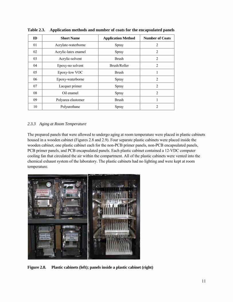
Table 2.3. Application methods and number of coats for the encapsulated panels

ID Short Name Application Method Number of Coats

01 Acrylate-waterborne Spray 2

02 Acrylic-latex enamel Spray 2

03 Acrylic-solvent Brush 2

04 Epoxy-no solvent Brush/Roller 2

05 Epoxy-low VOC Brush 1

06 Epoxy-waterborne Spray 2

07 Lacquer primer Spray 2

08 Oil enamel Spray 2

09 Polyurea elastomer Brush 1

10 Polyurethane Spray 2

2.3.3 Aging at Room Temperature

The prepared panels that were allowed to undergo aging at room temperature were placed in plastic cabinets housed in a wooden cabinet (Figures 2.8 and 2.9). Four separate plastic cabinets were placed inside the wooden cabinet, one plastic cabinet each for the non-PCB primer panels, non-PCB encapsulated panels, PCB primer panels, and PCB encapsulated panels. Each plastic cabinet contained a 12-VDC computer cooling fan that circulated the air within the compartment. All of the plastic cabinets were vented into the chemical exhaust system of the laboratory. The plastic cabinets had no lighting and were kept at room temperature.

Figure 2.8. Plastic cabinets (left); panels inside a plastic cabinet (right)

11

Figure 2.9. Wooden cabinets that housed the plastic cabinets

2.3.4 Accelerated Aging

Accelerated aging was performed on the prepared panels using a QUV Accelerated Weathering Tester (Q-Lab Corporation, Westlake, OH) (Figure 2.10). The tester was placed in a stainless steel tunnel to ventilate any possible PCB emissions to the exhaust system of the laboratory. The QUV tester contained eight 4-ft UVA-340 lamps (four on each side) and four UV monitoring sensors. The lamps emitted a peak wavelength of 340 nm. The irradiance for the device was set to 0.89 W/m2/nm for each test. Both sides of the tester held 12 racks, each containing two test panels. The irradiance of the QUV tester was calibrated using a CR-10 Calibration Radiometer (Q- Lab Corporation, Westlake, OH) prior to testing.

Figure 2.10. QUV Accelerated Weathering Tester: exterior (left); UV lamps (right)

12

It should be noted that the QUV chamber maintains a constant temperature during a test. Thus, the chamber cannot be used to evaluate the effect of temperature changes that could occur during normal diurnal and seasonal changes.

2.4 Sampling and Analysis

2.4.1 Internal Standards and Recovery Check Standards

Three 13C-labeled PCB congeners were used as the internal standards (ISs): 13C12-PCB-4, 13C12-PCB-52, and 13C12-PCB-194 (Wellington Laboratories, Shawnee Mission, KS). The internal standard solution for spiking contained 10 µg/mL of each IS.

Three chlorinated compounds were used as the recovery check standards (RCSs): 2,4,5,6-tetrachloro-m-xylene or TMX (Ultra Scientific, North Kingstown, RI), 13C12-PCB-77, and 13C12-PCB-206 (Wellington Laboratories, Shawnee Mission, KS). The RCS solution for spiking contained 5 µg/mL of each RCS.

2.4.2 Air Sampling

For the sink test, air samples were collected onto PUF sampling cartridges (pre-clean certified, Supelco, St. Louis, MO) by using a mass flow controller (Model FC-269, Coastal Instruments, Burgaw, NC) and a vacuum pump (Model 2565B-50, Welch, Skokie, IL). The sampling flow rate was set by the mass flow controller and measured by using a Gilian Gilibrator-2 Air Flow Calibrator (Scientific Instrument Services, Ringoes, NJ) before and after each sampling period. After the sample was collected, the glass holder with the sample inside was wrapped in a sheet of aluminum foil, placed in a sealable plastic bag, and stored in the refrigerator at 4 °C until extraction. Two field samples were collected during the sink tests and the results are presented in Table 3.5.

PUF samples were extracted using Soxhlet systems by following EPA Method 8082A (U.S. EPA, 2007). The PUF samples were placed in individual Soxhlet extractors with about 250 mL of hexane (ultra grade or equivalent, Fisher Scientific, Pittsburgh, PA). Fifty microliters of recovery check standards were spiked onto the PUF samples inside the Soxhlet extractor. The samples were extracted for 16 to 24 h. The extract was concentrated to about 50 to 75 mL using a Snyder column. The concentrated solution was then filtered through anhydrous sodium sulfate into a 100-mL borosilicate glass tube and further concentrated to about 1 mL using a RapidVap N2 Evaporation System (Model 791000, Labconco Corporation, Kansas City, MO). The 1-mL solution was cleaned with sulfuric acid (certified plus grade or equivalent, Fisher, Pittsburgh, PA) and brought up to 5 mL with the rinse solution (i.e., hexane for rinsing the concentration tube) in a 5 mL volumetric flask. One milliliter of the 5-mL solution was separated and spiked with 10 µL of the internal standard solution, after which the extract was transferred to GC vials for analysis by GC/MS. The final sample contained 50 ng/mL of each RCS and 100 ng/mL of each IS.

2.4.3 Extraction of Encapsulant-Coated Disks

The encapsulant-coated disks that were removed from the test chamber were extracted by using a modified sonication method (Guo et al., 2011). The disks were extracted for 30 min in a scintillation vial with 10 mL hexane (ultra grade or equivalent, Fisher Scientific, Pittsburgh, PA) and approximately 100 mg of sodium sulfate (anhydrous grade or equivalent, Fisher Scientific, Pittsburgh, PA) using a sonicator (Ultrasonic

13

Cleaner FS30, Fisher Scientific, Pittsburgh, PA). Before extraction, 100 µL of the recovery check standard solution were added to the extraction solution. After extraction, 990 µL of the extract was placed in a 1-mL volumetric flask containing 10 µL of the internal standard solution and the contents of the volumetric flask were transferred to GC vials for analysis. The final sample contained 50 ng/mL of each RCS and 100 ng/mL of each IS.

The sonication method was chosen for solid samples because (1) its extraction efficiency is as good as the Soxhlet method for the particular sample types associated with this study; (2) sonication involves fewer steps than the Soxhlet method, reducing the possibility of sample losses; (3) sonication consumes much less solvent. A disadvantage of the sonication method is that it cannot extract large samples such as the PUF samples.

2.4.4 Wipe Sampling

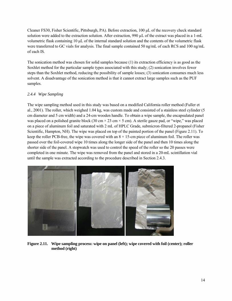
The wipe sampling method used in this study was based on a modified California roller method (Fuller et al., 2001). The roller, which weighed 1.04 kg, was custom made and consisted of a stainless steel cylinder (5 cm diameter and 5 cm width) and a 24-cm wooden handle. To obtain a wipe sample, the encapsulated panel was placed on a polished granite block (30 cm × 23 cm × 5 cm). A sterile gauze pad, or “wipe,” was placed on a piece of aluminum foil and saturated with 2 mL of HPLC Grade, submicron-filtered 2-propanol (Fisher Scientific, Hampton, NH). The wipe was placed on top of the painted portion of the panel (Figure 2.11). To keep the roller PCB-free, the wipe was covered with an 8 × 15-cm piece of aluminum foil. The roller was passed over the foil-covered wipe 10 times along the longer side of the panel and then 10 times along the shorter side of the panel. A stopwatch was used to control the speed of the roller so the 20 passes were completed in one minute. The wipe was removed from the panel and stored in a 20-mL scintillation vial until the sample was extracted according to the procedure described in Section 2.4.3.

Figure 2.11. Wipe sampling process: wipe on panel (left); wipe covered with foil (center); roller method (right)

14

Evaluation of this method showed that 2-propanol had a collection efficiency similar to that of hexane and that the use of aluminum foil on top of the wipe did not affect the collection efficiency. Details are presented in Appendix A.

The wipe sampling method described above was developed exclusively for this study to achieve better precision and repeatability than the commonly-used hand-wipe method. This wipe sampling method is not recommended for other uses.

2.4.5 Sample Analysis

The analytical method used in this project was a modification of EPA Method 8082A (U.S. EPA, 2007) and EPA Method 1668B (U.S. EPA, 2008a). The procedures are detailed in Part 1 of this report series (Guo et al., 2011).

15

3. Quality Assurance and Quality Control

Quality assurance (QA) and quality control (QC) procedures were implemented in this project by following the guidelines and procedures detailed in the approved Category II Quality Assurance Project Plan (QAPP), Polychlorinated Biphenyls (PCBs) in Caulk: Evaluation of coatings for encapsulating building materials contaminated by polychlorinated biphenyls (PCBs) and a NASA method for PCB destruction. Quality control samples consisted of background samples collected prior to the test, field blanks, spiked field controls, and duplicates. Daily calibration check samples were analyzed on each instrument on each day that analyses were conducted. The QA/QC activities and results that are specific to this study are described in Section 3.1. Data that did not meet the data quality indicators (DQIs) specified in the QAPP were not presented. Data quality indicators (DQIs) are presented in the first report of this report series (Guo et al., 2011).

The wipe samples presented in Sections 4.2.4 and 4.2.5 were analyzed by a commercial analytical laboratory. The QA/QC procedures and data quality evaluation for those samples are discussed in Section 3.2.

3.1 QA/QC for the In-house Analytical Laboratory

3.1.1 GC/MS Instrument Calibration

The GC/MS calibration and quantitation of PCBs were performed by using the relative response factor (RRF) method based on peak areas of extracted ion current profiles for target analytes relative to those of the internal standard. The calibration standards (AccuStandards, New Haven, CT) were prepared at six concentrations, ranging approximately from 5 to 200 ng/mL in hexane. Three internal standards were added in each standard solution for different PCB congeners. The calibration curve was obtained by injecting 1 µL of the prepared standards in triplicate at each concentration level. Table 3.1 summarizes all GC/MS calibrations conducted for the project, including the practical quantification limit (PQL, i.e., the lowest calibration concentration) and the highest calibration concentration. The percent relative standard deviation (RSD) of the average RRF met the data quality indicator (DQI) goal of 25%.

The Internal Audit Program (IAP) was implemented to minimize systematic errors. Prepared by personnel other than the analyst, the IAP standards contained three calibrated PCB congeners and were analyzed after the calibration was completed. The IAP standards were purchased from a supplier (ChemService,West Chester, PA) that was different from the supplier for the calibration standards, and the concentrations of PCB congeners in the standards were certified.

Table 3.2 presents the results of the analysis of the IAP standards for each calibration. The recoveries of the IAP standards ranged from 80% to 115% and the percent RSDs ranged from 0.13% to 1.40%. All the results met the criteria for IAP analysis, i.e., within 100 ± 25% of recovery and 25% of RSDs for triplicate analyses.

16

3.1.2 Detection Limits

After each calibration, the lowest calibration standard was analyzed seven times, and the instrument detection limit (IDL) was determined from three times the standard deviations of the measured concentrations of the standard. The IDLs for all calibrated PCB congeners are listed in Table 3.3. The detection limits for the sonication method were reported in the report entitled Laboratory Study of Polychlorinated Biphenyl (PCB) Contamination and Mitigation in Buildings, Part 2. Transport from Primary Sources to Building Materials and Settled Dust (Guo et al., 2012).

Table 3.1. GC/MS calibration for PCB congeners from Aroclor 1254 [a]

Date 2/14/2011 7/18/2011 12/21/2011 PQL

(ng/mL) Hi Cal [b]

(ng/mL) Analytes RRF %RSD RRF %RSD RRF %RSD

PCB-17 0.69 6.14 0.84 9.37 0.76 9.35 5.00 200

PCB-52 1.05 3.53 1.11 8.22 1.10 3.10 5.01 200

PCB-101 0.90 7.86 0.98 7.48 0.86 8.43 5.01 200

PCB-154 0.90 7.80 0.94 8.19 0.83 8.02 4.98 199

PCB-110 1.18 12.1 1.25 7.83 1.13 11.8 5.01 200

PCB-77 1.21 19.0 1.39 11.9 1.23 17.7 5.01 200

PCB-66 1.07 7.22 1.39 8.24 1.17 8.65 5.03 201

PCB-118 1.03 10.9 1.31 7.96 0.94 12.3 5.05 202

PCB-105 0.95 11.0 1.07 8.44 0.86 12.3 5.00 200

PCB-187 0.68 9.78 0.70 8.54 0.61 10.4 4.98 199

TMX (RCS) 0.40 4.11 0.46 5.89 0.44 3.04 5.01 200 13C12-PCB-77 (RCS) 1.12 16.7 1.20 15.5 1.00 18.6 5.00 200

13C12-PCB-206 (RCS) 1.08 11.5 1.03 7.42 0.98 13.5 5.00 200

[a] The Data Quality Indicator (DQI) goal for %RSD was 25%. [b] High calibration concentration.

17

Table 3.2. IAP results for each calibration related to this study [a]

Calibration Analyte IAP Concentration (ng/mL)

Avg. Recovery %

%RSD (n=3)

PCB-52 100 104 0.13

2/14/2011 PCB-101 100 94 0.33

PCB-77 100 80 0.64

PCB-52 80.0 116 0.38

7/18/2011 PCB-101 80.0 104 1.20

PCB-77 80.0 94 1.40

PCB-52 40.0 115 0.36

12/21//2011 PCB-101 40.0 103 0.41

PCB-77 40.0 91 1.22 [a] The DQI goal for IAP recovery was 75% to 125%.

Table 3.3. Instrument detection limits (IDLs) for PCB congeners on GC/MS (ng/mL)

Analytes 2/14/2011 7/18/2011 12/21/2011

PCB-17 0.69 0.40 1.28

PCB-52 0.32 0.26 0.15

PCB-101 0.35 0.52 0.47

PCB-154 0.47 0.58 0.59

PCB-110 0.38 0.45 0.51

PCB-77 0.41 0.42 0.67

PCB-66 0.13 0.34 0.54

PCB-118 0.23 0.47 0.58

PCB-105 0.24 0.31 0.52

PCB-187 0.26 0.37 0.69

TMX (RCS) 0.43 0.34 0.35 13C12-PCB-77 (RCS) 0.21 0.30 0.62

13C12-PCB-206 (RCS) 0.44 1.33 0.54

3.1.3 Environmental Parameters

The temperature and relative humidity (RH) sensors used to measure environmental conditions for the small chamber sink test were calibrated in EPA’s Metrology Laboratory in July, 2010. Environmental data in the small chamber, such as temperature and RH, were recorded by the OPTO 22 data acquisition system (DAS).

18

The air exchange rate of the small chamber was calculated based on the average flow rate of outlet air measured with a Gilibrator at the start and end of each test in the small chamber. The Gilibrator was calibrated by EPA’s Metrology Laboratory. The environmental parameters that were measured are presented in Table 4.1 in Section 4.1.1. The data met the data quality goals.

The accelerated weathering chamber (QUV chamber) was set to be operated at a 340 nm irradiance of 0.89 W/m2/nm) and 60 °C. A CR-10 Calibration Radiometer (Q-Lab Corporation, Westlake, OH) was used to calibrate the irradiance of the QUV chamber prior to each test. The device was connected to the appropriate port on the QUV control panel. Lamp type UV-A was selected on the radiometer, and the sensor was placed into the calibration port on the back panel of the chamber. Following the appropriate procedural steps, the radiometer automatically calibrated and updated the irradiance of the sensor to 0.89 W/m2/nm. The process was repeated for all four sensors on the QUV chamber. The CR-10 manufacturer, Q-Lab, calibrated the radiometer on 10/23/2009. The temperature and relative humidity in the QUV chamber were not monitored.

3.1.4 Quality Control Samples

The quality control samples discussed here include background, field blank, method blank, and replicate samples.

A typical background sample showed the contribution of the contamination in the empty chamber, the sampling device, and the clean air supply. The results of the sink tests are summarized in Table 3.4. Some of the PCB concentrations in the small chamber tests were above the PQL, possibly due to carryover from previous tests. These high backgrounds did not affect the test results because the PCB concentrations in chamber air were monitored (See Figure 4.1) and because they can be considered as part of the source for the test chamber. No background samples were collected for the QUV chambers.

Table 3.4. Background concentrations of PCBs (µg/m3) in the chamber for the sink test[a]

Analyte Empty chamber Chamber with substrate

PCB-17 0.08 0.02

PCB-52 3.17 0.58

PCB-101 0.70 0.21

PCB-154 0.25 0.02

PCB-110 0.00 0.11

PCB-77 0.11 0.00

PCB-66 0.06 0.03

PCB-118 0.01 0.04

PCB-105 0.00 0.01

PCB-187 0.00 0.00 [a] Values in strikethrough are below PQL.

19

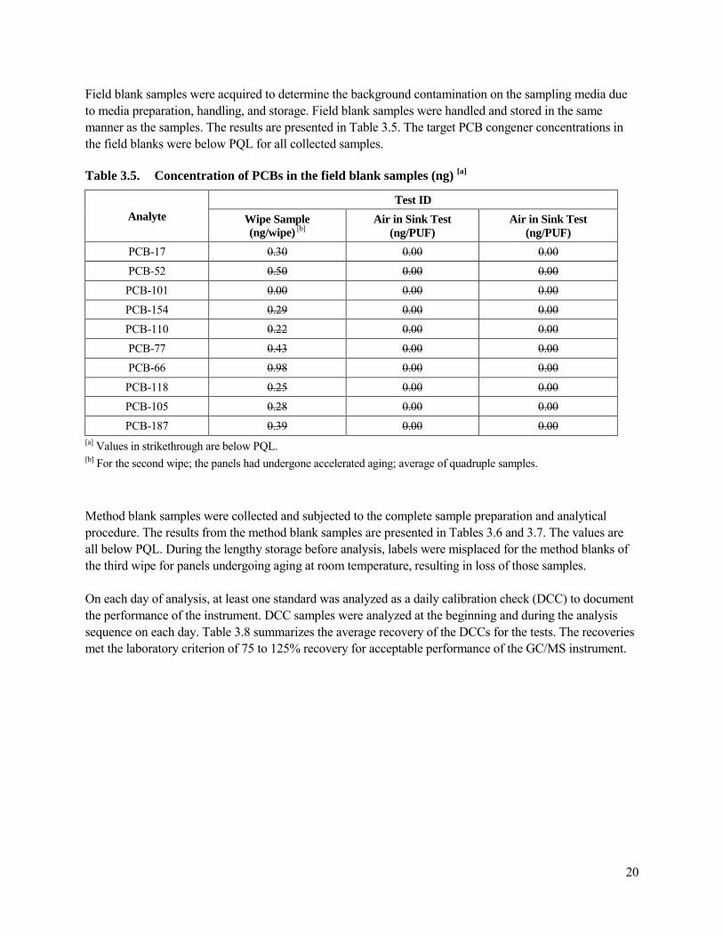
Field blank samples were acquired to determine the background contamination on the sampling media due to media preparation, handling, and storage. Field blank samples were handled and stored in the same manner as the samples. The results are presented in Table 3.5. The target PCB congener concentrations in the field blanks were below PQL for all collected samples.

Table 3.5. Concentration of PCBs in the field blank samples (ng) [a]

Analyte Test ID

Wipe Sample (ng/wipe) [b]

Air in Sink Test (ng/PUF)

Air in Sink Test (ng/PUF)

PCB-17 0.30 0.00 0.00 PCB-52 0.50 0.00 0.00

PCB-101 0.00 0.00 0.00

PCB-154 0.29 0.00 0.00 PCB-110 0.22 0.00 0.00 PCB-77 0.43 0.00 0.00 PCB-66 0.98 0.00 0.00

PCB-118 0.25 0.00 0.00 PCB-105 0.28 0.00 0.00 PCB-187 0.39 0.00 0.00

[a] Values in strikethrough are below PQL. [b] For the second wipe; the panels had undergone accelerated aging; average of quadruple samples.

Method blank samples were collected and subjected to the complete sample preparation and analytical procedure. The results from the method blank samples are presented in Tables 3.6 and 3.7. The values are all below PQL. During the lengthy storage before analysis, labels were misplaced for the method blanks of the third wipe for panels undergoing aging at room temperature, resulting in loss of those samples.

On each day of analysis, at least one standard was analyzed as a daily calibration check (DCC) to document the performance of the instrument. DCC samples were analyzed at the beginning and during the analysis sequence on each day. Table 3.8 summarizes the average recovery of the DCCs for the tests. The recoveries met the laboratory criterion of 75 to 125% recovery for acceptable performance of the GC/MS instrument.

20

Table 3.6. Concentration of PCBs in the method blank samples (µg/cm2 wipe sample) for the accelerated weathering process [a][b]

Analyte Sample Batch / Wipe Sample ID

Batch 1 Third Wipe

Batch 2 Third Wipe

Batch 2 Fourth Wipe

Batch 3 First Wipe

Batch 3 Second Wipe

Batch 3 Third Wipe

PCB-17 0.00 0.00 0.00 0.00 0.00 0.00 PCB-52 0.00 0.00 0.00 0.00 0.00 0.00 PCB-101 0.00 0.00 0.00 0.00 0.00 0.00 PCB-154 0.00 0.00 0.00 0.00 0.00 0.00 PCB-110 0.00 0.00 0.00 0.00 0.00 0.00 PCB-77 0.00 0.00 0.00 0.00 0.00 0.00 PCB-66 0.00 0.00 0.00 0.00 0.00 0.00 PCB-118 0.00 0.00 0.00 0.00 0.00 0.00 PCB-105 0.00 0.00 0.00 0.00 0.00 0.00 PCB-187 0.00 0.00 0.00 0.00 0.00 0.00

[a] Values in strikethrough are below PQL. [b] Average of quadruple samples.

Table 3.7. Concentration of PCBs in the method blank samples (µg/cm2 wipe sample) for panels in the storage cabinet [a][b]

Analyte

Sample Batch / Wipe Sample ID

Batch 2A[c]

Third Wipe Batch 2B[d]

Third Wipe Batch 2A[c]

Fourth Wipe Batch 2B[d]

Fourth Wipe

PCB-17 0.00 0.00 0.00 0.00 PCB-52 0.00 0.00 0.00 0.00

PCB-101 0.00 0.00 0.00 0.00 PCB-154 0.00 0.00 0.00 0.00 PCB-110 0.00 0.00 0.00 0.00 PCB-77 0.00 0.00 0.00 0.00 PCB-66 0.00 0.00 0.00 0.00

PCB-118 0.00 0.00 0.00 0.00 PCB-105 0.00 0.00 0.00 0.00 PCB-187 0.00 0.00 0.00 0.00

[a] Values in strikethrough are below PQL. [b] Average of duplicate samples. [c] For panels that had undergone accelerated aging. [d] For panels that had undergone aging at room temperature.

21

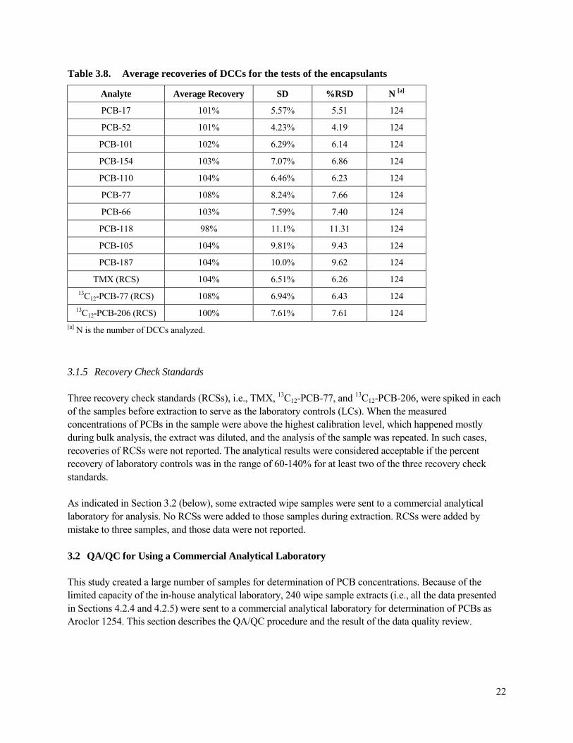
Table 3.8. Average recoveries of DCCs for the tests of the encapsulants

Analyte Average Recovery SD %RSD N [a]

PCB-17 101% 5.57% 5.51 124

PCB-52 101% 4.23% 4.19 124

PCB-101 102% 6.29% 6.14 124

PCB-154 103% 7.07% 6.86 124

PCB-110 104% 6.46% 6.23 124

PCB-77 108% 8.24% 7.66 124

PCB-66 103% 7.59% 7.40 124

PCB-118 98% 11.1% 11.31 124

PCB-105 104% 9.81% 9.43 124

PCB-187 104% 10.0% 9.62 124

TMX (RCS) 104% 6.51% 6.26 124 13C12-PCB-77 (RCS) 108% 6.94% 6.43 124

13C12-PCB-206 (RCS) 100% 7.61% 7.61 124 [a] N is the number of DCCs analyzed.

3.1.5 Recovery Check Standards

Three recovery check standards (RCSs), i.e., TMX, 13C12-PCB-77, and 13C12-PCB-206, were spiked in each of the samples before extraction to serve as the laboratory controls (LCs). When the measured concentrations of PCBs in the sample were above the highest calibration level, which happened mostly during bulk analysis, the extract was diluted, and the analysis of the sample was repeated. In such cases, recoveries of RCSs were not reported. The analytical results were considered acceptable if the percent recovery of laboratory controls was in the range of 60-140% for at least two of the three recovery check standards.

As indicated in Section 3.2 (below), some extracted wipe samples were sent to a commercial analytical laboratory for analysis. No RCSs were added to those samples during extraction. RCSs were added by mistake to three samples, and those data were not reported.

3.2 QA/QC for Using a Commercial Analytical Laboratory

This study created a large number of samples for determination of PCB concentrations. Because of the limited capacity of the in-house analytical laboratory, 240 wipe sample extracts (i.e., all the data presented in Sections 4.2.4 and 4.2.5) were sent to a commercial analytical laboratory for determination of PCBs as Aroclor 1254. This section describes the QA/QC procedure and the result of the data quality review.

22

3.2.1 QA/QC Procedure

The commercial analytical laboratory that we selected was certified by the National Environmental Laboratory Approval Program (NELAP), and it specializes in the analysis of PCBs (Aroclors and congeners) by GC/ECD and GC/MS using standard analytical methods. EPA SW-846 Method 8082 (U.S. EPA, 2008b) was used for the wipe samples reported in Section 4.2.4 and 4.2.5.

Five QC samples were included in each batch of samples sent to the commercial analytical laboratory for the determination of PCB content. The QC samples were not the same set for different batches. These QC samples included:

• Two certified Aroclor 1254 standard solutions for evaluating the accuracy of the analytical results.

• Two aliquots of the same hexane extract solution for evaluating the precision of the analytical results.

• One solvent blank for determining the presence of any potential sample contamination in the laboratory and during transportation.

3.2.2 Data Quality Indicators (DQIs)

The data quality indicators (DQIs) presented in Table 3.9 were defined before receiving any data from the commercial laboratory.

Table 3.9. Criteria for determining the usability of data reported by the commercial laboratory

Purpose DQI

Data usability

Accepted as quantitative data

Accepted as semi-quantitative data

Disqualified

Accuracy Relative error (Er) [a] |Er| ≤ 25% 25% < |Er| < 50% |Er| ≥ 50%

Precision RSD [b] RSD ≤ 25% 25% < RSD < 50% RSD ≥ 50%

Laboratory contamination Solvent blank (C0) C0 ≤ PQL PQL < C0 < 2 PQL C0 ≥ 2 PQL

[a] Based on analysis of certified Aroclor 1254 standards: Er = (reported value – certified value) / certified value. [b] Based on analysis of two aliquots of the same hexane extract.

3.2.3 Data Quality Evaluation

The results for the accuracy, precision, and solvent blank analyses are presented in Tables 3.10 through 3.12.

The laboratory used tetrachloro-m-xylene (TCMX) and PCB congener #209 as the recovery check standards (RCSs), and the recoveries of the RCSs were satisfactory (Table 3.13).

23

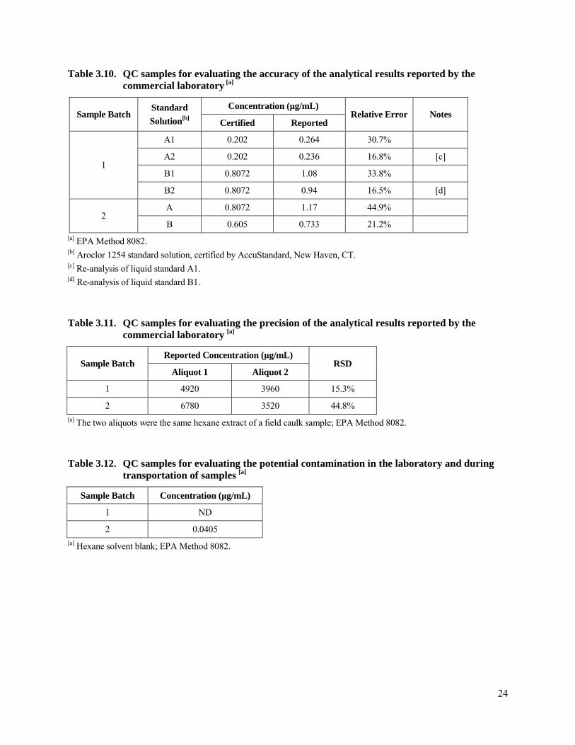
Table 3.10. QC samples for evaluating the accuracy of the analytical results reported by the commercial laboratory [a]

Sample Batch Standard

Solution[b]

Concentration (µg/mL) Relative Error Notes

Certified Reported

1

A1 0.202 0.264 30.7%

A2 0.202 0.236 16.8% [c]

B1 0.8072 1.08 33.8%

B2 0.8072 0.94 16.5% [d]

2 A 0.8072 1.17 44.9%

B 0.605 0.733 21.2% [a] EPA Method 8082. [b] Aroclor 1254 standard solution, certified by AccuStandard, New Haven, CT. [c] Re-analysis of liquid standard A1. [d] Re-analysis of liquid standard B1.

Table 3.11. QC samples for evaluating the precision of the analytical results reported by the commercial laboratory [a]

Sample Batch Reported Concentration (µg/mL)

RSD Aliquot 1 Aliquot 2

1 4920 3960 15.3%

2 6780 3520 44.8% [a] The two aliquots were the same hexane extract of a field caulk sample; EPA Method 8082.

Table 3.12. QC samples for evaluating the potential contamination in the laboratory and during transportation of samples [a]

Sample Batch Concentration (µg/mL)

1 ND

2 0.0405 [a] Hexane solvent blank; EPA Method 8082.

24

Table 3.13. Recovery of the recovery check standards (RCSs) for all wipe samples analyzed by the commercial laboratory

Sample Group Total No. of

Samples

RCS recovery between 60% and 140%

TCMX PCB-209

No. of Samples % of Total No. of Samples % of Total

Aging room temperature 120 116 96.7% 116 96.7%

Accelerated aging 119 [a] 118 99.2% 118 99.2% [a] One missing sample excluded.

3.2.4 Conclusion Related to Data Quality Review

Judging from the pre-defined DQIs in Table 3.9 and the results of the analyses of the QC samples presented in Tables 3.10 through 3.13, the wipe sample data presented in Sections 4.2.4 and 4.2.5 had uncertainties between 25% and 50% as estimated based on the accuracy and the precision of the QC samples and, thus, should be considered to be semi-quantitative (See Table 3.9). The data is still useful to compare the relative performance of the encapsulants because the PCB concentrations in wipe samples covered a range of more than an order of magnitude for the encapsulants evaluated.

25

4. Experimental Results

4.1 Sink Tests

4.1.1 Test Conditions

The conditions of the test chamber are shown in Table 4.1. The test duration was 433 hours. The thicknesses of the dry films of the encapsulants are presented in Table 4.2. The concentrations of the target PCB congeners in the air of the test chamber are shown in Figures 4.1 and 4.2.

Table 4.1. Conditions of the test chamber

Parameter Mean [a] SD

Temperature (˚C) 23.2 0.08

Relative humidity (%) 46.0 1.34

Air change rate (h-1) 1.05 0.01 [a] n = 1684.

Table 4.2. Thicknesses of the dry films of the encapsulants used for the sink test

Coating ID

Coating Name

Film Thickness (mm)

Mean[a] SD

01 Acrylate-waterborne 0.095 0.009

02 Acrylic-latex enamel 0.067 0.026

03 Acrylic-solvent 0.305 0.052

04 Epoxy-low VOC 0.399 0.092

05 Epoxy-no solvent 0.501 0.156

06 Epoxy-waterborne 0.168 0.015

07 Lacquer primer 0.191 0.060

08 Oil enamel 0.127 0.043

09 Polyurea elastomer 1.63 0.298

10 Polyurethane 0.056 0.022 [a] n = 24 for each encapsulant.

26

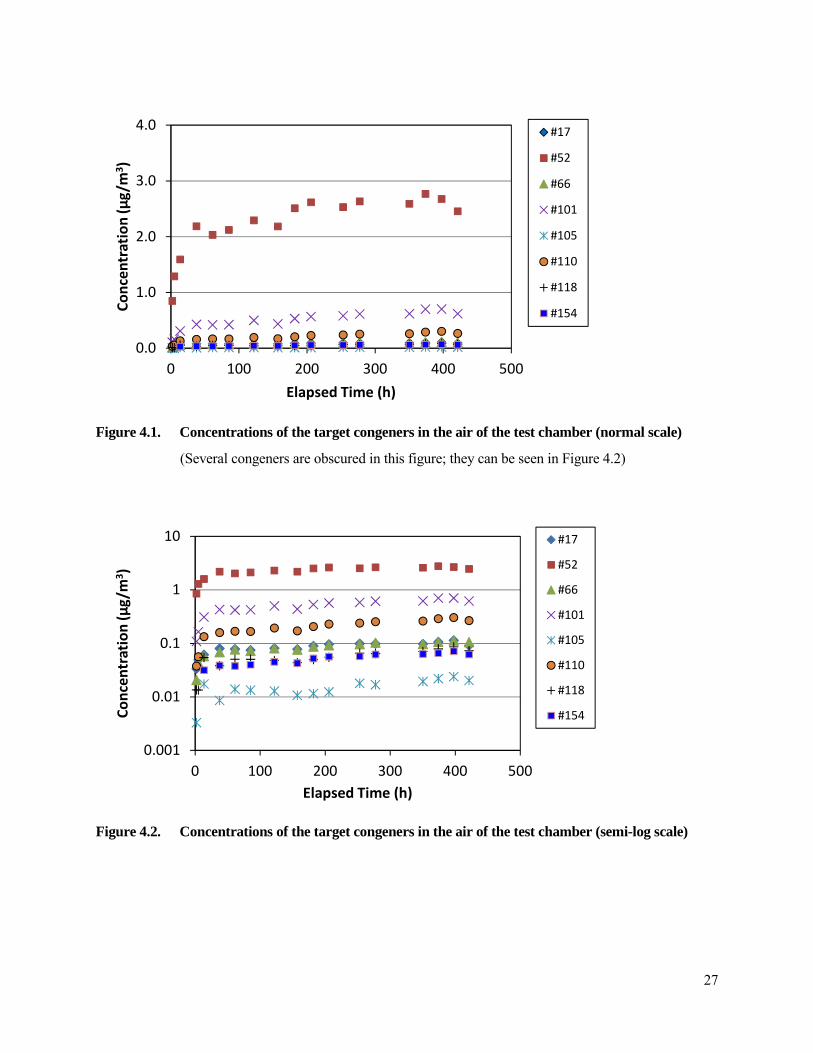
4.0

3.0

2.0

1.0

0.0

Elapsed Time (h)

0 100 200 300 400 500

#17

#52

#66

#101

#105

#110

#118

#154

Co

nce

ntr

ati

on

(μ

g/m

3)

Figure 4.1. Concentrations of the target congeners in the air of the test chamber (normal scale)

(Several congeners are obscured in this figure; they can be seen in Figure 4.2)

Co

nce

ntr

ati

on

(μ

g/m

3)

10

1

0.1

0.01

0.001

#17

#52

#66

#101

#105

#110

#118

#154

0 100 200 300 400 500 Elapsed Time (h)

Figure 4.2. Concentrations of the target congeners in the air of the test chamber (semi-log scale)

27

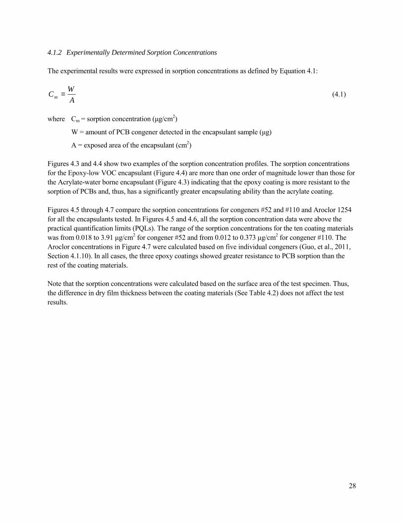
4.1.2 Experimentally Determined Sorption Concentrations

The experimental results were expressed in sorption concentrations as defined by Equation 4.1:

WC = (4.1) m A

where Cm = sorption concentration (µg/cm2)

W = amount of PCB congener detected in the encapsulant sample (µg)

A = exposed area of the encapsulant (cm2)

Figures 4.3 and 4.4 show two examples of the sorption concentration profiles. The sorption concentrations for the Epoxy-low VOC encapsulant (Figure 4.4) are more than one order of magnitude lower than those for the Acrylate-water borne encapsulant (Figure 4.3) indicating that the epoxy coating is more resistant to the sorption of PCBs and, thus, has a significantly greater encapsulating ability than the acrylate coating.

Figures 4.5 through 4.7 compare the sorption concentrations for congeners #52 and #110 and Aroclor 1254 for all the encapsulants tested. In Figures 4.5 and 4.6, all the sorption concentration data were above the practical quantification limits (PQLs). The range of the sorption concentrations for the ten coating materials was from 0.018 to 3.91 µg/cm2 for congener #52 and from 0.012 to 0.373 µg/cm2 for congener #110. The Aroclor concentrations in Figure 4.7 were calculated based on five individual congeners (Guo, et al., 2011, Section 4.1.10). In all cases, the three epoxy coatings showed greater resistance to PCB sorption than the rest of the coating materials.

Note that the sorption concentrations were calculated based on the surface area of the test specimen. Thus, the difference in dry film thickness between the coating materials (See Table 4.2) does not affect the test results.

28

2.0 )

2m PCB-17c �

/g

μ PCB-52 �( 1.5

noi PCB-66 �

tart PCB-101

ne 1.0 c PCB-105 n

oC PCB-110

noit 0.5 PCB-118

pro

S PCB-154

0.0 0 100 200 300 400 500

Elapsed Time (h)

10

) 2 PCB-17�

mc/g PCB-52 �

μ 1

( n PCB-66 �

oita PCB-101

rtn 0.1

e PCB-105

cn

o PCB-110

C n

o PCBi 0.01 -118

tpr PCB-154

oS

0.001 0 100 200 300 400 500

Elapsed Time (h)Title

Figure 4.3. Experimentally-determined sorption concentrations as a function of time for the Acrylate-waterborne coating material (top: normal scale; bottom: semi-log scale).

29

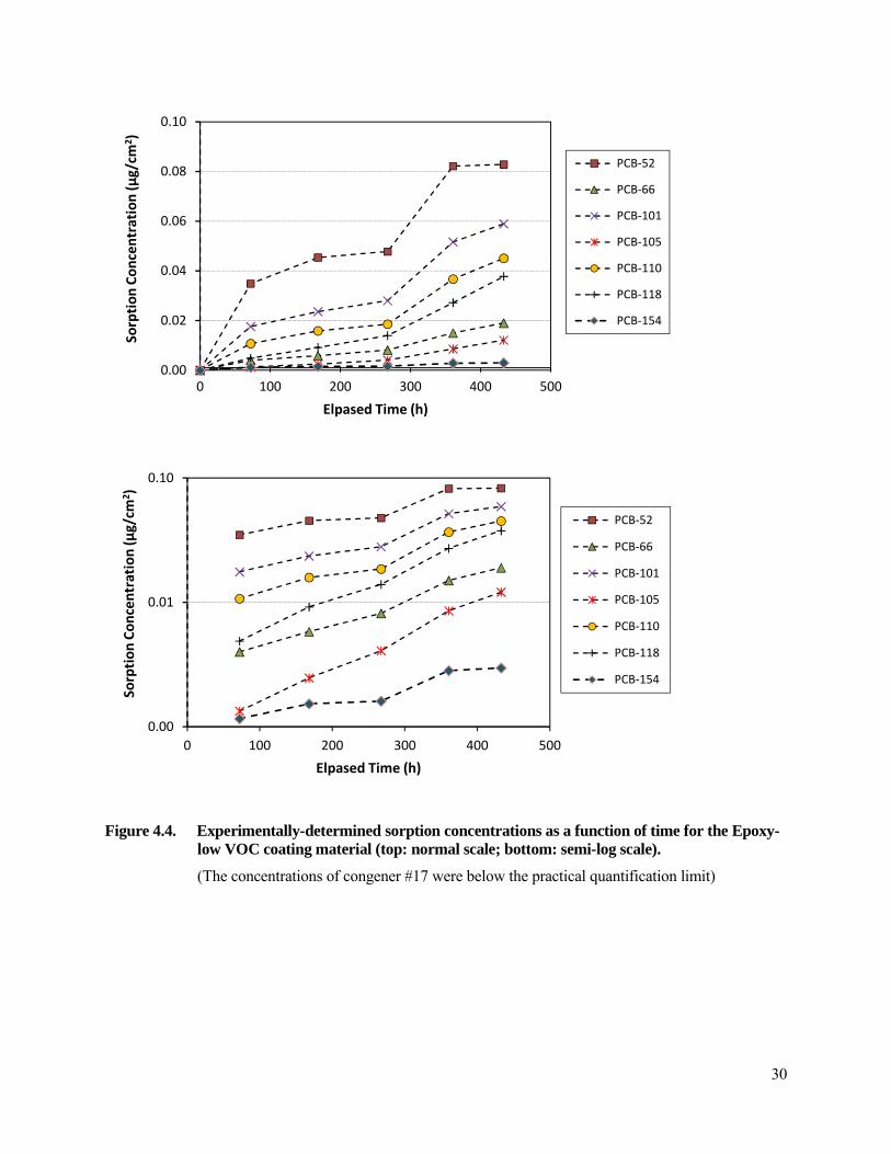
0.10

PCB-52 0.08

PCB-66

PCB-101 0.06 PCB-105

PCB-110

PCB-118

0.04

PCB-154 0.02

0.00 0 100 200 300 400 500

Elpased Time (h)

0.10

PCB-52

PCB-66

PCB-101

PCB-105

PCB-110

PCB-118

PCB-154

0.01

0.00 0 100 200 300 400 500

Elpased Time (h)

So

rpti

on

Co

nce

ntr

ati

on

(μ

g/c

m2)

S

orp

tio

n C

on

cen

tra

tio

n (

μg

/cm

2)

Figure 4.4. Experimentally-determined sorption concentrations as a function of time for the Epoxy-low VOC coating material (top: normal scale; bottom: semi-log scale).

(The concentrations of congener #17 were below the practical quantification limit)

30

0.0

1.0

2.0

3.0

4.0

5.0

So

rpti

on

Co

nce

ntr

ati

on

(μ

g/c

m2

) Congener #52

Figure 4.5. Experimentally-determined sorption concentrations for congener #52 for the ten encapsulants (t = 433 h)

0.0

0.1

0.2

0.3

0.4

So

rpti

on

Co

nce

ntr

ati

on

(μ

g/c

m2

)

Congener #110

Figure 4.6. Experimentally-determined sorption concentrations for congener #110 for the ten encapsulants (t = 433 h)

31

_ _

_ _

0

5

10

15

20

25

So

rpti

on

Co

nce

ntr

ati

on

(μ

g/c

m2

) Aroclor 1254

Figure 4.7. Calculated sorption concentrations for Aroclor 1254 for the ten encapsulants (t = 433 h)

4.1.3 Estimation of the Partition and Diffusion Coefficients

The experimentally-determined sorption concentrations were used to estimate the material/air partition coefficients and solid-phase diffusion coefficients for the ten encapsulants. The two parameters were estimated by fitting a mass transfer model to the experimental data by non-linear regression. The details of this parameter estimation method are described in Part 2 of this report series (Guo et al., 2012, Appendix C). The estimated partition and diffusion coefficients and calculated sink sorption indices (SSIs) for conger #52 ― the reference congener ― for the ten encapsulants are presented in Table 4.3. Figure 4.8 shows how well the model fit the experimental data. The relative standard deviations (RSDs) for the estimated partition coefficients ranged from 8.8 to 67% based on three estimates; the RSD range for the diffusion coefficients was from 18% to 92%. Thus, the results should be considered rough estimates.

Selection of the reference congener is arbitrary. In this study, congener #52 was selected as the reference congener because of its abundance in the air and in the sink material (Guo et al., 2012, Section 6.2.4). The coefficients for the other congeners can be calculated from Equations 4.2 and 4.3:

α P0

Pi

K K (4.2) =

ma i 0ma

β m0

mi

D D (4.3) =

m i 0m

where Kma_i = material/air partition coefficient for congener i (dimensionless) Kma_0 = material/air partition coefficient for the reference congener (dimensionless) P0 = vapor pressure for the reference congener (torr)

32

Pi = vapor pressure for congener i (torr) α = material-dependent constant from Table 4.3 Dm_i = solid-phase diffusion coefficient for congener i (m2/h) Dm_0 = solid-phase diffusion coefficient for the reference congener (m2/h) m0 = molecular weight of the reference congener (g/mol) mi = molecular weight of congener i (g/mol) β = 6.5 for all materials.

Once the material/air partition coefficients for two materials are known, the material/material partition coefficient of the two materials can be calculated from Equation 4.4 (Kumar and Little, 2003). The material/material partition coefficient is a key parameter that controls the migration of PCBs from the source to the encapsulant.

Kma _1K12 = (4.4) Kma _ 2

where K12 = material/material coefficient between material 1 and material 2 (dimensionless) Kma_1 = material/air partition coefficient for material 1 (dimensionless) Kma_2 = material/air partition coefficient for material 2 (dimensionless)

0 100 200 300 400 500

Elapsed Time (h)

Figure 4.8. Goodness-of-fit for estimating the partition and diffusion coefficients for the Acrylic-solvent coating material

(The lines are model fit; the symbols are experimental data; r2 is the overall coefficient of determination for the non-linear regression)

0.0

1.0

2.0

3.0

4.0

5.0

So

rpti

on

Am

ou

nt

(μg

)

#52

#101

#110

#154

r2 = 0.985

33

Table 4.3. Estimated partition coefficient (Kma), diffusion coefficient (Dm) for the reference congener (#52) and index α in Equation 4.2 [a]

Encapsulant Kma (Dimensionless) Dm (m2/h) α (Dimensionless)

r2 [b] SSI [c]

ID Name Mean RSD Mean RSD Mean RSD Mean RSD

01 Acrylate-waterborne 1.93×107 29.4% 4.88×10-10 58.6% 0.418 0.0% 0.9814 2.0 6.8%

02 Acrylic-latex enamel 2.05×107 19.6% 1.75×10-10 36.0% 0.582 0.0% 0.9849 2.4 3.6%

03 Acrylic-solvent 1.34×107 35.9% 2.06×10-10 73.8% 0.646 0.0% 0.9922 2.6 6.7%

04 Epoxy-low VOC 3.05×106 57.2% 3.76×10-11 72.2% 0.912 5.8% 0.9544 3.9 6.6%

05 Epoxy-no solvent [d] 1.78×106 62.3% 1.89×10-12 92.0% 1.007 0.0% 0.9741 5.5 12.2%

06 Epoxy-waterborne 2.02×106 67.1% 8.36×10-12 75.9% 0.981 5.0% 0.9819 4.8 7.2%

07 Lacquer primer 7.90×106 20.6% 9.50×10-11 45.3% 0.829 0.0% 0.9854 3.1 3.2%

08 Oil enamel 1.62×107 35.7% 4.53×10-10 60.1% 0.478 0.0% 0.9981 2.1 7.5%

09 Polyurea elastomer 1.78×107 9.5% 1.34×10-09 18.0% 0.232 0.0% 0.9502 1.6 5.2%

10 Polyurethane 5.93×106 8.8% 1.12×10-10 19.4% 0.896 0.0% 0.9887 3.2 3.0% [a] The mean and RSD values were based on three estimates. [b] Overall coefficient of determination for the non-linear regression. [c] SSI is sink sorption index; SSI = -log (Kma Dm), from Guo et al. (2012). [d] Most sorption concentration data were below the PQLs for this encapsulant.

34

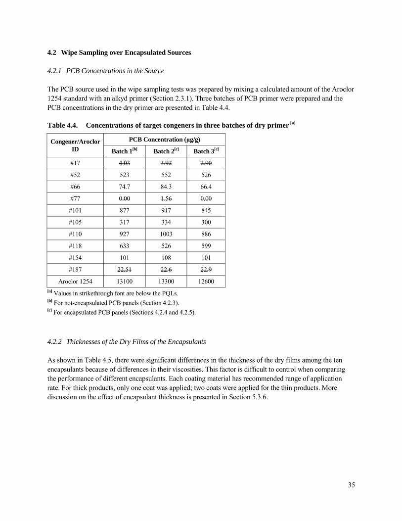
4.2 Wipe Sampling over Encapsulated Sources

4.2.1 PCB Concentrations in the Source

The PCB source used in the wipe sampling tests was prepared by mixing a calculated amount of the Aroclor 1254 standard with an alkyd primer (Section 2.3.1). Three batches of PCB primer were prepared and the PCB concentrations in the dry primer are presented in Table 4.4.

Table 4.4. Concentrations of target congeners in three batches of dry primer [a]

Congener/Aroclor ID

PCB Concentration (µg/g)

Batch 1[b] Batch 2[c] Batch 3[c]

#17 4.03 3.92 2.90

#52 523 552 526

#66 74.7 84.3 66.4

#77 0.00 1.56 0.00

#101 877 917 845

#105 317 334 300

#110 927 1003 886

#118 633 526 599

#154 101 108 101

#187 22.51 22.6 22.9

Aroclor 1254 13100 13300 12600 [a] Values in strikethrough font are below the PQLs. [b] For not-encapsulated PCB panels (Section 4.2.3). [c] For encapsulated PCB panels (Sections 4.2.4 and 4.2.5).

4.2.2 Thicknesses of the Dry Films of the Encapsulants

As shown in Table 4.5, there were significant differences in the thickness of the dry films among the ten encapsulants because of differences in their viscosities. This factor is difficult to control when comparing the performance of different encapsulants. Each coating material has recommended range of application rate. For thick products, only one coat was applied; two coats were applied for the thin products. More discussion on the effect of encapsulant thickness is presented in Section 5.3.6.

35

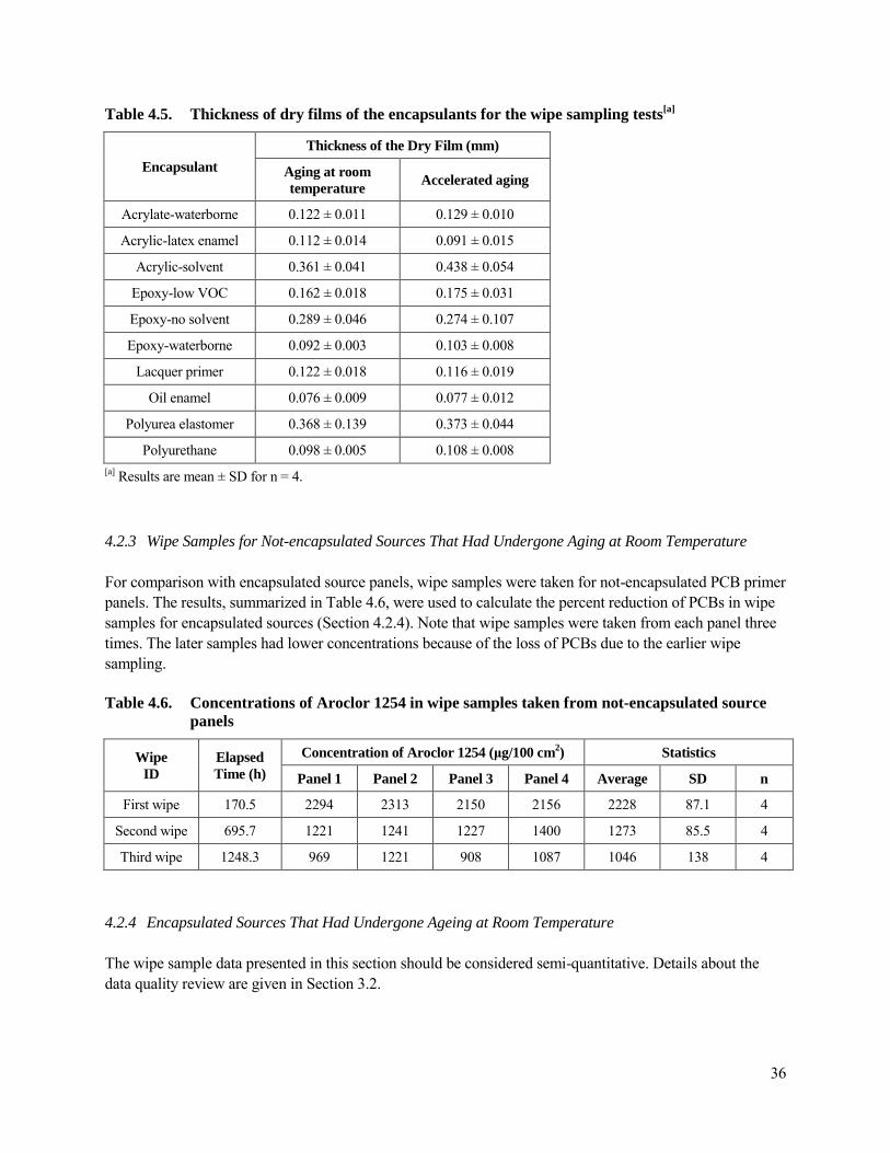
Table 4.5. Thickness of dry films of the encapsulants for the wipe sampling tests[a]

Encapsulant

Thickness of the Dry Film (mm)

Aging at room temperature

Accelerated aging

Acrylate-waterborne 0.122 ± 0.011 0.129 ± 0.010

Acrylic-latex enamel 0.112 ± 0.014 0.091 ± 0.015

Acrylic-solvent 0.361 ± 0.041 0.438 ± 0.054

Epoxy-low VOC 0.162 ± 0.018 0.175 ± 0.031

Epoxy-no solvent 0.289 ± 0.046 0.274 ± 0.107

Epoxy-waterborne 0.092 ± 0.003 0.103 ± 0.008

Lacquer primer 0.122 ± 0.018 0.116 ± 0.019

Oil enamel 0.076 ± 0.009 0.077 ± 0.012

Polyurea elastomer 0.368 ± 0.139 0.373 ± 0.044

Polyurethane 0.098 ± 0.005 0.108 ± 0.008 [a] Results are mean ± SD for n = 4.

4.2.3 Wipe Samples for Not-encapsulated Sources That Had Undergone Aging at Room Temperature

For comparison with encapsulated source panels, wipe samples were taken for not-encapsulated PCB primer panels. The results, summarized in Table 4.6, were used to calculate the percent reduction of PCBs in wipe samples for encapsulated sources (Section 4.2.4). Note that wipe samples were taken from each panel three times. The later samples had lower concentrations because of the loss of PCBs due to the earlier wipe sampling.

Table 4.6. Concentrations of Aroclor 1254 in wipe samples taken from not-encapsulated source panels

Wipe Elapsed Concentration of Aroclor 1254 (µg/100 cm2) Statistics

ID Time (h) Panel 1 Panel 2 Panel 3 Panel 4 Average SD n

First wipe 170.5 2294 2313 2150 2156 2228 87.1 4

Second wipe 695.7 1221 1241 1227 1400 1273 85.5 4

Third wipe 1248.3 969 1221 908 1087 1046 138 4

4.2.4 Encapsulated Sources That Had Undergone Ageing at Room Temperature

The wipe sample data presented in this section should be considered semi-quantitative. Details about the data quality review are given in Section 3.2.

36

The PCB concentrations, as Aroclor 1254, in the three rounds of wipe samples are presented in Figures 4.9 through 4.11. Figure 4.12 compares the sum of three rounds of wipe sampling for the encapsulants and the relative contribution of each wipe to the total amount of PCBs collected in three wipes. The ranking of the ten encapsulants based on wipe sampling showed some resemblance to the results of the sink tests (Figure 4.7). The three epoxy coatings performed well in both tests. Although the two types of tests were based on completely different mass transfer mechanisms (i.e., migration from a solid source versus deposition from the air), such consistency demonstrates that these tests are useful for evaluating the performance of different encapsulants.

Polyurea-elastomer was an obvious exception. This encapsulant showed the worst performance in the sink test but had very good performance in wipe sampling. The difference in the thickness of the encapsulants in the wipe sampling tests may have contributed partially to this discrepancy. As shown in Table 4.5, the Polyurea-elastomer was the thickest among all the encapsulants tested. Results of mathematical modeling presented in Section 5.3.6 show that, for a given source and a given encapsulant, the PCB concentration at the exposed surface decreases when the thickness of the encapsulant increases. Thus, increased thickness reduces the PCB concentration at the exposed surface. In future tests, this coating material should be further evaluated.

0

200

400

600

800

Aro

clo

r 1

25

4 (

μg

/10

0 c

m2

)

t = 167 hours

Figure 4.9. Concentration of Aroclor 1254 in the first-round wipe samples taken over encapsulated PCB panels that had undergone aging at room temperature (error bar = ±1 SD)

37

0

200

400

600

800 A

rocl

or

12

54

(μ

g/1

00

cm

2 )

t ≈ 600 hours

Figure 4.10. Concentrations of Aroclor 1254 in the second-round wipe samples taken over encapsulated PCB panels that had undergone aging room temperature (error bar = ±1 SD)

0

200

400

600

800

Aro

clo

r 1

25

4 (

μg

/10

0 c

m2

) t ≈ 1500 hours

Figure 4.11. Concentrations of Aroclor 1254 in the third-round wipe samples taken over encapsulated PCB panels that had undergone aging at room temperature (error bar = ±1 SD)

38

Aro

clo

r 1

25

4 (

μg

/10

0 c

m2) 1600

1200

800

400

0

Wipe 3

Wipe 2

Wipe 1

Figure 4.12. Concentrations of Aroclor 1254 for the sum of three rounds of wipe samples taken over encapsulated PCB panels that had undergone aging at room temperature

The percent reduction of PCBs in the wipe samples for the encapsulated sources was calculated by using Equation 4.5:

C − C% Reduction = 0 x × 100% (4.5) C0

where C0 = PCB concentration in the wipe sample for the not-encapsulated source panel (µg/100 cm2)

Cx = PCB concentration in the wipe sample for the encapsulated source panel (µg/100 cm2)

As shown in Table 4.7, the percent reduction for the ten encapsulants ranged from 40.3% to 99.9%.

39

Table 4.7 Percent reduction of PCB concentrations in wipe samples for encapsulated PCB sources

Encapsulant ID

Encapsulant

Percent Reduction of Aroclor 1254 in Wipe Samples

Wipe 1 Wipe 2 Wipe 3

01 Oil enamel 86.1% 77.3% 74.2%

02 Epoxy-low VOC 98.4% 99.0% 100.0%

03 Epoxy-waterborne 94.3% 97.3% 99.8%

04 Acrylate-waterborne 89.8% 80.1% 69.3%

05 Acrylic-latex enamel 77.9% 67.3% 40.3%

06 Acrylic-solvent 89.6% 89.6% 86.1%

07 Lacquer primer 73.8% 73.8% 72.0%

08 Polyurethane 89.4% 82.7% 98.7%

09 Epoxy-no solvent 99.5% 99.1% 99.9%

10 Polyurea elastomer 97.2% 93.6% 99.2%

4.2.5 Encapsulated Sources That Had Undergone Accelerated Aging

The wipe sample data presented in this section should be considered semi-quantitative. Details about the data quality review are presented in Section 3.2.

The concentrations of Aroclor 1254 in the wipe samples taken from the panels that had undergone accelerated aging were significantly lower than those from the panels that had undergone aging at room temperature. Over half of the wipe samples had concentrations in the noise level of the analytical method (Figures 4.13 through 4.17). One possible cause of this difference may have been the elevated temperature (60 ˚C) in the QUV chamber. During the two-week period of testing, PCBs may have been driven off the source surface in significant quantities. Although the test results are difficult to interpret, the following observations can still be made:

• The epoxy coatings and the polyurea elastomer performed well relative to other encapsulants, consistent with the results from aging at room temperature.

• The main purpose of the accelerated aging tests was to determine whether degradation of the encapsulant may cause increased concentrations of PCBs at the encapsulated surface. The test results did not indicate any such effect.

UV irradiation is a key factor that causes degradation of polymers in the coating materials. Given that the UV intensity inside buildings is much lower than in the ambient environment, the degradation of coating materials is much slower indoors than outdoors. Thus, in most cases, the degradation of coating materials is not a primary concern for PCB encapsulants inside buildings. Weathering of the encapsulant could be a concern, however, if the source is on the exterior side of the building.

40

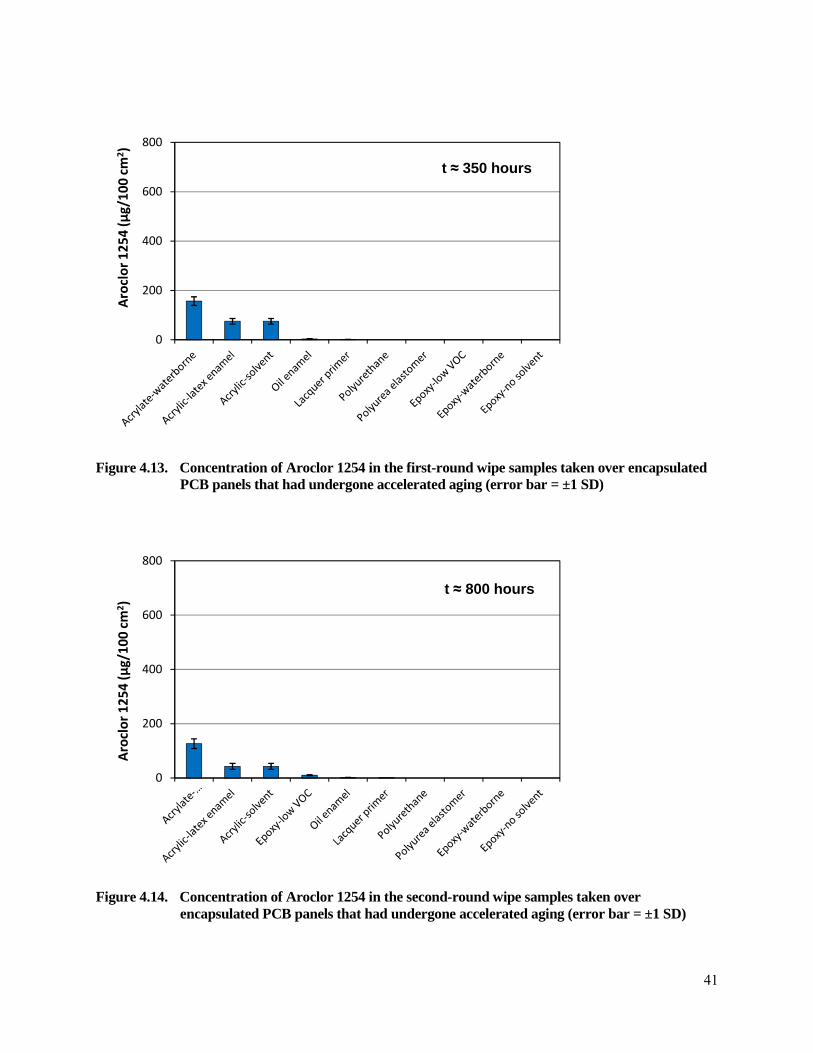
0

200

400

600

800

Aro

clo

r 1

25

4 (

μg

/10

0 c

m2

)

t ≈ 350 hours

Figure 4.13. Concentration of Aroclor 1254 in the first-round wipe samples taken over encapsulated PCB panels that had undergone accelerated aging (error bar = ±1 SD)

0

200

400

600

800

Aro

clo

r 1

25

4 (

μg

/10

0 c

m2

)

t ≈ 800 hours

Figure 4.14. Concentration of Aroclor 1254 in the second-round wipe samples taken over encapsulated PCB panels that had undergone accelerated aging (error bar = ±1 SD)

41

0

200

400

600

800 A

rocl

or

12

54

(μ

g/1

00

cm

2 )

t ≈ 1500 hours

Figure 4.15. Concentration of Aroclor 1254 in the third-round wipe samples taken over encapsulated PCB panels that had undergone accelerated aging (error bar = ±1 SD)

0

400

800

1200

1600

Aro

clo

r 1

25

4 (

μg

/10

0 c

m2

)

Wipe 3

Wipe 2

Wipe 1

Figure 4.16. Concentrations of Aroclor 1254 for the sum of three rounds of wipe samples taken over encapsulated PCB panels that had undergone accelerated aging

42

0

500

1000

1500

2000

Aro

clo

r 1

25

4 (

μg

/10

0 c

m2

) Natural aging

Accelerated aging

Figure 4.17. Comparison of wipe sampling results (the sum of three wipes) for the two aging methods

4.2.6 Additional Wipe Sampling Tests

4.2.6.1 Effect of the Thickness of the Encapsulant

The effect of the thickness of the encapsulant on the PCB concentration in wipe samples was evaluated by applying one and two coats of an encapsulant to the same types of source panels. The test conditions were as follows:

PCB source Alkyd primer mixed with 0.71% of Aroclor 1254

Substrate 6 in × 3 in (15.2 cm × 7.6 cm) aluminum panels

Source area 51.8 ± 0.42 cm2 (n = 6)

Encapsulant Acrylic-solvent

Thickness of encapsulant 0.277 ± 0.032 mm (n = 3) for one coat

0.441 ± 0.045 mm (n = 3) for two coats

Application method roller

Aging method At room temperature without lighting

Wipe sampling times 167, 692, and 1245 elapsed hours

For a given source and a given encapsulant, the test results show that the PCB concentration in the wipe samples decreases as the thickness of the dry film of the encapsulant increases (Figures 4.18 through 4.21).

43

Co

ng

en

er

Co

nc.

(μ

g/1

00

cm

2)

40

30

20

10

0

One coat

Two coats

#52 #66 #101 #105 #110 #118 #154 #187

Congener ID

Figure 4.18. Concentrations of target congeners in wipe samples taken at 167 elapsed hours

(The encapsulant was Acrylic-solvent; error bar = ±1 SD)

40

Co

ng

en

er

Co

nc.

(μ

g/1

00

cm

2)

30

20

10

0

One coat

Two coats

#52 #66 #101 #105 #110 #118 #154 #187

Congener ID

Figure 4.19. Concentrations of target congeners in wipe samples taken at 692 elapsed hours

(The encapsulant was Acrylic-solvent; error bar = ±1 SD)

44

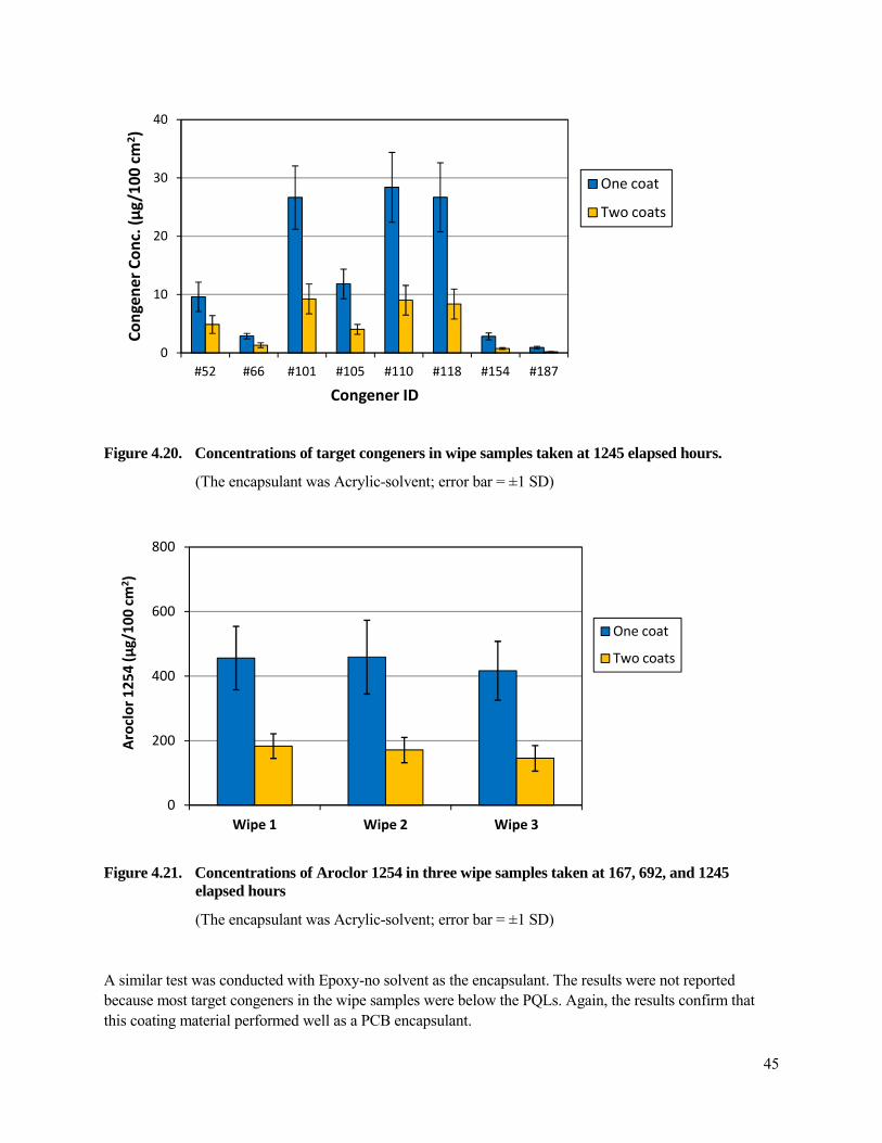
Co

ng

en

er

Co

nc.

(μ

g/1

00

cm

2)

40

30

20

10

0

Congener ID

#52 #66 #101 #105 #110 #118 #154 #187

One coat

Two coats

Figure 4.20. Concentrations of target congeners in wipe samples taken at 1245 elapsed hours.

(The encapsulant was Acrylic-solvent; error bar = ±1 SD)

800

Aro

clo

r 1

25

4 (

μg

/10

0 c

m2)

600

400

200

0

One coat

Two coats

Wipe 1 Wipe 2 Wipe 3�

Figure 4.21. Concentrations of Aroclor 1254 in three wipe samples taken at 167, 692, and 1245 elapsed hours

(The encapsulant was Acrylic-solvent; error bar = ±1 SD)

A similar test was conducted with Epoxy-no solvent as the encapsulant. The results were not reported because most target congeners in the wipe samples were below the PQLs. Again, the results confirm that this coating material performed well as a PCB encapsulant.

45

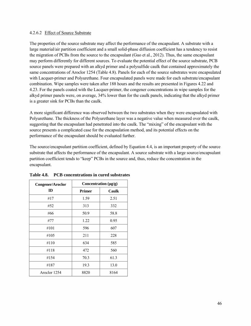
4.2.6.2 Effect of Source Substrate

The properties of the source substrate may affect the performance of the encapsulant. A substrate with a large material/air partition coefficient and a small solid-phase diffusion coefficient has a tendency to resist the migration of PCBs from the source to the encapsulant (Guo et al., 2012). Thus, the same encapsulant may perform differently for different sources. To evaluate the potential effect of the source substrate, PCB source panels were prepared with an alkyd primer and a polysulfide caulk that contained approximately the same concentrations of Aroclor 1254 (Table 4.8). Panels for each of the source substrates were encapsulated with Lacquer-primer and Polyurethane. Four encapsulated panels were made for each substrate/encapsulant combination. Wipe samples were taken after 188 hours and the results are presented in Figures 4.22 and 4.23. For the panels coated with the Lacquer-primer, the congener concentrations in wipe samples for the alkyd primer panels were, on average, 34% lower than for the caulk panels, indicating that the alkyd primer is a greater sink for PCBs than the caulk.

A more significant difference was observed between the two substrates when they were encapsulated with Polyurethane. The thickness of the Polyurethane layer was a negative value when measured over the caulk, suggesting that the encapsulant had penetrated into the caulk. The “mixing” of the encapsulant with the source presents a complicated case for the encapsulation method, and its potential effects on the performance of the encapsulant should be evaluated further.

The source/encapsulant partition coefficient, defined by Equation 4.4, is an important property of the source substrate that affects the performance of the encapsulant. A source substrate with a large source/encapsulant partition coefficient tends to “keep” PCBs in the source and, thus, reduce the concentration in the encapsulant.

Table 4.8. PCB concentrations in cured substrates

Congener/Aroclor Concentration (µg/g)

ID Primer Caulk

#17 1.59 2.51

#52 313 332

#66 50.9 58.8

#77 1.22 0.95

#101 596 607

#105 211 228

#110 634 585

#118 472 560

#154 70.3 61.3

#187 19.3 13.0

Aroclor 1254 8820 8164

46

15 )

2 Primer

m 12

c0

Caulk

0/1

g 9

μ(n

oit

a 6

rtn

ecn

o 3

C

0

#52 #105 #101 #110 #118

Congener ID

Figure 4.22. Effect of source substrate on PCB concentrations in wipe samples ― the sources (primer and caulk) were encapsulated with the Lacquer-primer (error bar = ±1 SD)

40

Co

nce

ntr

ati

on

(μ

g/1

00

cm

2)

30

20

10

0

Primer

Caulk

#52 #105 #101 #110 #118 #154

Congener ID

Figure 4.23. Effect of source substrate on PCB concentrations in wipe samples ― the sources (primer and caulk) were encapsulated with Polyurethane (error bar = ±1 SD)

47

5. Mathematical Modeling

5.1 Model Description

5.1.1 Available Barrier Models

Barrier models are mass transfer models for predicting the behavior of encapsulated sources. Several models are available for evaluating the effect of the barrier layer on emissions of chemical substances from solid building materials (Little et al., 2002; Kumar and Little, 2003; Hu et al., 2007; Yuan et al., 2007). The first barrier model (Little et al., 2002) gives the exact solution to the case in which the barrier material is applied to one side of the source panel. Unfortunately, one parameter in the model (CL2) was either mistyped or undefined. The model developed by Kumar and Little (2003) is for predicting the rate of mass transfer between a double-layer material and indoor air. The model is in the form of the exact solutions and the material can be either a source or a sink. The model developed by Hu et al. (2007) provides a generalized form of the exact solutions to the emissions from multi-layered building materials. The model developed by Yuan et al. (2007) is a fugacity model for layered materials. As a barrier model, it works for cases in which the barrier material is applied to either one or two sides of the source panel. The model is solved numerically. In this study, the fugacity model was used to investigate the general behavior of encapsulated sources, and the factors that affect the performance of the encapsulants. It was also used to rank the ten encapsulants that were tested.

5.1.2 The Concept of Fugacity

Fugacity can be regarded as the “escaping tendency” of a chemical substance from an environmental compartment or phase (Mackay and Paterson, 1981). The fugacity of a chemical is linked to its concentration, as shown in Equation 5.1:

C = Z F (5.1)

where C = concentration of the chemical in the compartment (mol/m3)

Z = fugacity capacity of the compartment for the chemical [mol/(m3 Pa)]

F = fugacity of the chemical in the compartment (Pa)

Fugacity capacity (Z) is an important parameter that dictates the movement of contaminants between environmental compartments. The contaminants tend to accumulate in the compartments with large fugacity capacities. The direction of the flux of the contaminant between two compartments is determined by the fugacity difference between the two compartments (i.e., from the compartment with a higher fugacity to the compartment with a lower fugacity).

One of the advantages of the fugacity models over conventional concentration models is the continuity of the fugacity at the interface of the two compartments because such continuity often simplifies the numerical computations, especially when the model includes partial differential equations.

48

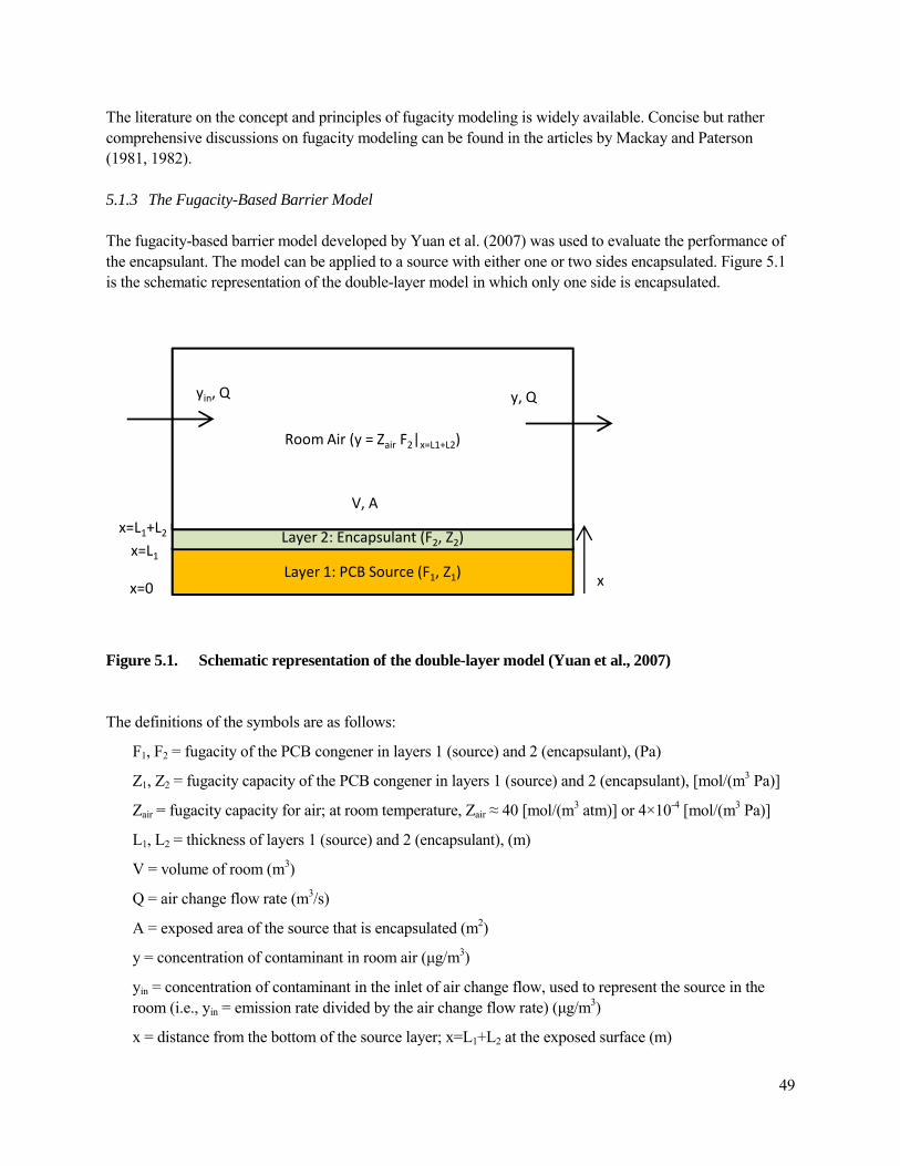
The literature on the concept and principles of fugacity modeling is widely available. Concise but rather comprehensive discussions on fugacity modeling can be found in the articles by Mackay and Paterson (1981, 1982).

5.1.3 The Fugacity-Based Barrier Model

The fugacity-based barrier model developed by Yuan et al. (2007) was used to evaluate the performance of the encapsulant. The model can be applied to a source with either one or two sides encapsulated. Figure 5.1 is the schematic representation of the double-layer model in which only one side is encapsulated.

Layer 1: PCB Source (F1, Z1)

Layer 2: Encapsulant (F2, Z2)

Room Air (y = Zair F2|x=L1+L2)

yin, Q y, Q

V, A

x

x=L1

x=L1+L2

x=0

Figure 5.1. Schematic representation of the double-layer model (Yuan et al., 2007)

The definitions of the symbols are as follows:

F1, F2 = fugacity of the PCB congener in layers 1 (source) and 2 (encapsulant), (Pa)

Z1, Z2 = fugacity capacity of the PCB congener in layers 1 (source) and 2 (encapsulant), [mol/(m3 Pa)]

Zair = fugacity capacity for air; at room temperature, Zair ≈ 40 [mol/(m3 atm)] or 4×10-4 [mol/(m3 Pa)]

L1, L2 = thickness of layers 1 (source) and 2 (encapsulant), (m)

V = volume of room (m3)

Q = air change flow rate (m3/s)

A = exposed area of the source that is encapsulated (m2)

y = concentration of contaminant in room air (µg/m3)

yin = concentration of contaminant in the inlet of air change flow, used to represent the source in the room (i.e., yin = emission rate divided by the air change flow rate) (µg/m3)

x = distance from the bottom of the source layer; x=L1+L2 at the exposed surface (m)

49

The model was developed with the following assumptions: (1) There is no contaminant flux through the bottom layer (Equation 5.2); (2) The air in the room is well mixed and, thus, the mass balance for the contaminant in room air can be established (Equation 5.3, which can be converted to Equation 5.4 and then to Equation 5.5); (3) The contaminant at the surface of the top layer is always in equilibrium with the room air (Equation 5.6); (4) The contact between the two layers is perfect and, thus, the fugacity at the interface is continuous (Equations 5.7 and 5.8).

∂ F1 = 0 (5.2) ∂ x

x=0

∂ y ∂ F2= Q y + D AZ − Q y (5.3) in 2 2∂ t ∂ x

∂ F2 ∂ F2 V Z = Q Z F + D AZ − Q Z F (5.4) air air in 2 2 air 2∂ t ∂ x

∂ F ∂ FD 2 − k 2 − h D F + h D F = 0 , (5.5) 2 2 2 2 2 2 2 in ∂ x ∂ t

where F = y / Zin in air

Qh2 =

A K2 D2

Vk2 =

A K2

K = Z2 / Z2 air

(5.6) y = Z Fair 2 x=L +L1 2

(5.7) = F2F1 x=L x=L1 1

∂ F1 ∂ F2D Z = D Z (5.8) 1 1 2 2∂ x ∂ x ,

where D1 = diffusion coefficient for the contaminant in the source layer (m2/s)

D2 = diffusion coefficient for the contaminant in the barrier layer (m2/s)

K1 = material/air partition coefficient of the source layer for the contaminant (dimensionless)

50

K2 = material/air partition coefficient of the barrier layer for the contaminant (dimensionless)

Z1 = K1 Zair

Given the fugacities of the contaminants at time t = 0, Equations 5.5 and 5.8 can be solved numerically. The MATLAB code of the model used in this study was provided by Drs. John Little and Zhe Liu of Virginia Polytechnic Institute and State University, the co-authors of this model (Yuan et al., 2007).

5.2 Input Parameters

5.2.1 Parameters Required by the Model

This fugacity model requires 13 input parameters if one side of the source panel is encapsulated (Table 5.1). Among these parameters, the partition coefficients, diffusion coefficients, the initial concentration, and the film thickness of the encapsulant are the most important parameters. For air concentrations, the ventilation rate and source area are also important.

Table 5.1. Input parameters for the fugacity model

Parameter Symbol Unit

Exposed area of the source A m2

Thickness of the source layer L1 m

Thickness of the barrier layer L2 m

Molecular weight of the contaminant [a] MW µg/mol

Initial concentration of the contaminant in the source layer C01 µg/m3

Initial concentration of the contaminant in the barrier layer C02 µg/m3

Concentration of the contaminant in the inlet air [b] yin µg/m3

Material/air partition coefficient for the contaminant and source layer K1 dimensionless

Material/air partition coefficient for the contaminant and the barrier layer K2 dimensionless

Diffusion coefficient for the contaminant and in the source layer D1 m2/s

Diffusion coefficient for the contaminant and in the barrier layer D2 m2/s

Room volume V m3

Air change flow rate Q m3/s [a] For converting fugacity (Pa) to concentration (µg/m3). To convert the concentration in the solid material from (µg/m3) to (µg/g), the density of the material is required. [b] Parameter yin is also used to represent the emissions from other indoor sources.

5.2.2 Parameter Values for the “Base-case” Scenario

Table 5.2 lists the “base-case” values of nine parameters for use in all the simulations unless indicated otherwise. The remaining four parameters, the partition and diffusion coefficients for the source and encapsulant, are given in Table 5.3. The source material is assumed to be concrete and the encapsulant is

51

either Lacquer primer or Epoxy-waterborne. The values in Table 5.3 are for congener #110, the most abundant congener in Aroclor 1254.

Table 5.2. Base-case values for the simulations

Parameter Symbol Value Unit Notes

Exposed area of the source (concrete) A 10 m2

Thickness of the source layer L1 0.005 m = 5 mm [a]

Thickness of the barrier layer L2 0.0001 m = 0.1 mm

Molecular weight of the contaminant (congener #110) MW 3.27×108 µg/mol = 327 g/mol

Initial concentration of congener #110 in the source layer C01 2.00×108 µg/m3 = 100 µg/g

Initial concentration of congener #110 in the barrier layer C02 0 µg/m3

Concentration of congener #110 in the inlet air yin 0 µg/m3

Room volume V 100 m3

Air change flow rate Q 2.78×10-2 m3/s = 100 m3/h [a] This is not the thickness of the concrete structure; it is the thickness of the layer that is contaminated with PCBs.

Table 5.3. Partition coefficients (Kma) and diffusion coefficients (Dm) for congener #110 for the source and encapsulants [a]

Material Category Material Name Kma Dm (m2/s)

Source Concrete [a] 6.95 × 107 4.00 × 10-15

Encapsulant Epoxy-waterborne[b] 1.73 × 107 1.25 × 10-15

Lacquer primer[b] 4.85 × 107 1.28 × 10-14

[a] Data from Guo et al. (2012). [b] Calculated from Equations 4.2 and 4.3 using the data in Table 4.3.

To convert the concentrations in the solid phases from (µg/m3) to (µg/g), the density is assumed to be 2.0 g/cm3 for the source (concrete) and 1.2 g/cm3 for the encapsulant.

5.3 General Behavior of Encapsulated Sources

5.3.1 Concentration Profiles in the Source

Using the parameters in Tables 5.2 and 5.3 as input to the fugacity model described in Section 5.1.3, the concentration profiles in the source and encapsulant layers can be calculated. As shown in Figures 5.2 and 5.3, a concentration gradient develops at the interface of the source and the encapsulant (i.e., x = 5 mm), resulting in a decreased driving force for PCB migration from the source to the encapsulant. The development of the concentration gradient is faster for the Lacquer primer (Figure 5.2) than for the Epoxy (Figure 5.3) because the former has a greater diffusion coefficient (Table 5.3).

52

C1(

x) (

μg

/g)

120

80

100 1 day

10 days

20

40

60

Concrete / Lacquer-primer

100 days

1000 days

5000 days

0 0 1 2 3

x (mm) 4 5

120

100

C1(

x) (µ

g/g

) 80 1 day

10 days

60 100 days

40 1000 days

20 Concrete / Epoxy-waterborne

5000 days

0 0 1 2 3 4 5

x (mm)

Figure 5.2. Concentration profiles for congener #110 in the source encapsulated with a Lacquer-primer [C1(x)].

(The interface of the source and the encapsulant is at x = 5 mm; the initial concentration in the source (C01) was 100 µg/g.)

Figure 5.3. Concentration profiles for congener #110 in the source encapsulated with a waterborne epoxy coating [C1(x)]

(The interface of the source and the encapsulant is at x = 5 mm; the initial concentration in the source (C01) was 100 µg/g.)

53

5.3.2 Concentration Profiles in the Encapsulant Layer

The profile of the contaminant in the encapsulant layer is more complex than in the source (Figures 5.4 and 5.5). The accumulation of contaminant in the encapsulant is controlled by two factors, i.e., the gain due to the flux of the contaminant from the source and the loss due to emissions to room air. The net effects are: (1) the contaminant “fills up” the encapsulant layer quickly in the early days; (2) the concentration of the contaminant at x = 0 (i.e., the interface of the source and the encapsulant) decreases over time; and (3) the concentration of the contaminant at x = 0.1 (i.e., the surface of the encapsulant that is exposed to air) increases at first and then decreases over time.

The concentration at the interface of the source and the encapsulant (i.e., x = 0) is greater for the Lacquer than for the Epoxy because the former has a greater material/air partition coefficient. The concentration gradient in the encapsulant layer is steeper for the Epoxy than for the Lacquer because the former has a smaller diffusion coefficient.

80

Concrete / Lacquer-primer

0.00 0.02 0.04 0.06 0.08 0.10

60

40

1 day

10 days

100 days

1000 days

5000 days

C2(

x) (

ug

/g)

20

0

x (mm)

Figure 5.4. Concentration profiles for congener #110 in the encapsulant layer (Lacquer primer) as a function of depth

(The interface of the source and the encapsulant is at x = 0 mm; the exposed surface is at x = 0.1 mm; the initial concentration in the source (C01) was 100 µg/g)

54

55

0

10

20

30

40

50

0.00 0.02 0.04 0.06 0.08 0.10

C2(

x) (

μg

/g)

x (mm)

1 day

10 days

100 days

1000 days

10000 days

Concrete / Epoxy-waterborne

Figure 5.5. Concentration profiles for congener #110 in the encapsulant layer (Epoxy-waterborne) as a function of depth

(The interface of the source and the encapsulant is at x = 0 mm; the exposed surface is at x = 0.1 mm; the initial concentration in the source (C01) was 100 µg/g.)

5.3.3 Average Concentration in the Encapsulant Layer

With the concentration profiles shown in Figures 5.4 and 5.5, the average concentrations in the encapsulant can be calculated from Equation 5.9:

( )( )[ ]∑∫−

=++ −+≈=

1

01122

202

22 2

1)(1 2 n

iiiii

L

xxCCL

dxxCL

C (5.9)

where C2 = average concentration in the encapsulant layer (µg/g)

C2(x) = concentration in the encapsulant layer at depth x (µg/g)

L2 = thickness of the encapsulant layer (m)

C2i = the ith data point for C2(x), (µg/g)

C th2i+1 = the (i+1) data point for C2(x), (µg/g)

n+1 = number of data points.

Figure 5.6 shows the average concentration in the encapsulant layer as function of time. The contaminant accumulates in the encapsulant rapidly in the early hours, followed by a slow decrease. The decrease is

56

caused mainly by the concentration gradient formed at the interface of the source and the encapsulant (Figures 5.2 and 5.3).

0

20

40

60

0 1000 2000 3000 4000 5000

Ave

rag

e C

2(µ

g/g

)

Elapsed Time (days)

Lacquer primer

Epoxy-waterborne

Figure 5.6. The average concentration of congener #110 in the encapsulant layer (C2) as a function of time

(The initial concentration in the source, C01, was 100 µg/g.)

5.3.4 Concentration at the Exposed Surface

The PCB concentration on the exposed surface of the encapsulant is an important parameter for evaluating the performance of an encapsulant because the concentration at the surface is linked to dermal exposure and to the contribution of the encapsulated source to the PCB concentration in the air. As shown in Figure 5.7, a significant difference exists between the two encapsulants due to the combined effect of the partition and diffusion coefficients. Note that the concentration at the exposed surface (Figure 5.7) is always less than the average concentration in the encapsulant layer (Figure 5.6).

5.3.5 Contribution to PCB Concentrations in Room Air

One of the main goals of encapsulating PCB sources is to reduce the PCB concentrations in room air. Figure 5.8 shows the contribution of the encapsulated source to the PCB concentrations in room air. For comparison, the air concentration due to emissions from not-encapsulated concrete is also included. The difference between the two encapsulants is more significant in the short term than in the long term.

5.3.6 Effect of the Thickness of the Encapsulant

The effect of the thickness of the encapsulant on the average concentration in the encapsulant layer is complex. As shown in Figures 5.9 and 5.10, as the thickness increases, the average concentration increases at first and then decreases.

57

0

10

20

30

40

50

0 1000 2000 3000 4000 5000

C2(x

=L 2

) (μ

g/g

)

Elapsed Time (days)

Lacquer primer

Epoxy-waterborne

Figure 5.7. Concentration of congener #110 at the exposed surface of the encapsulant [C2(x=L2)] as a function of time

(The initial concentration in the source, C01, was 100 µg/g.)

0.0

1.0

2.0

3.0

0 1000 2000 3000 4000 5000

Air

co

nce

ntr

ati

on

(μ

g/m

3)

Elapsed Time (days)

Lacquer primer

Epoxy-waterborne

Not-encapsulated concrete

Figure 5.8. Concentration of congener #110 in room air due to emissions from the encapsulated source as a function of time

(The initial concentration in the source, C01, was 100 µg/g.)

Av

era

ge

C2

(μ

g/g

)

40

50

Concrete / Lacquer-primer

30

20

0

10

0.00 0.20 0.40

Thickness of Encapsulant (mm)

t = 100 days

t = 1000 days

0.60

Figure 5.9. Effect of the thickness of the encapsulant on the average concentration of congener #110 in the encapsulant layer (average C2) ― Case 1: Lacquer primer

25

Concrete / Epoxy-waterborne

20

Av

era

ge

C2

(μ

g/g

)

15

10

5 t = 100 days

t = 1000 days

0

0.0 0.1 0.2 0.3 0.4 0.5

Thickness of Encapsulant (mm)

0.6

Figure 5.10. Effect of the thickness of the encapsulant on the average concentration of congener #110 in the encapsulant layer (average C2) ― Case 2: Epoxy-waterborne

The effect of the thickness of the encapsulant on the concentration at the exposed surface is much simpler, i.e., as the thickness increases, the surface concentration decreases (Figures 5.11 and 5.12). The contribution of the encapsulated source to the concentrations of PCBs in room air follows a similar trend (Figures 5.13 and 5.14).

58

C2(x

=L2

) (μ

g/g

)

40

30

20

10

0

Concrete / Lacquer primer

t = 100 days

t = 1000 days

0.0 0.2 0.4 0.6

Thickness of Encapsulant (mm)

5

C2(x

=L 2

) (μ

g/g

)

4

3

2

1

0

t = 100 days

t = 1000 days

Concrete / Epoxy-waterborne

0.0 0.1 0.2 0.3 0.4 0.5 0.6

Thickness of Encapsulant (mm)

Figure 5.11. Effect of the thickness of the encapsulant on the concentration of congener #110 at the exposed surface of the encapsulant [C2(x=L2)] ― Case 1: Lacquer-primer

Figure 5.12. Effect of the thickness of the encapsulant on the concentration of congener #110 at the exposed surface of the encapsulant [C2(x=L2)] ― Case 2: Epoxy-waterborne

59

1.0 A

ir C

on

cen

tra

tio

n (

μg

/m3)

0.8 t = 100 days

t = 1000 days

0.6

0.4

0.0

0.2

0.0 0.1 0.2 0.3

Concrete / Lacquer primer

0.4 0.5 0.6

Thickness of Encapsulant (mm)

0.30

Co

nce

ntr

ati

o in

air

(μ

g/m

3)

0.25 Concrete / Epoxy-waterborne

0.15

0.20 t = 100 days

t = 1000 days

0.10

0.05

0.00

0.0 0.2 0.4 0.6

Thickness of Encapsulant (mm)

Figure 5.13. Effect of encapsulant thickness on the concentration of congener #110 in room air due to emissions from the encapsulated source ― Case 1: Lacquer-primer

Figure 5.14. Effect of encapsulant thickness on the concentration of congener #110 in room air due to emissions from the encapsulated source ― Case 2: Epoxy-waterborne

60

400

Lacquer primer

Av

era

ge

C2

(μ

g/g

) 300 Epoxy-waterborne

200

100

0

0 200 400 600 800 1000

Initial Concentration in Source (μg/g)

t = 100 days

1200

160

Lacquer primer

Av

era

ge

C2

(μ

g/g

) 120 Epoxy-waterborne

80

0

40

0 200 400 600 800 1000

Initial Concentration in Source (μg/g)

t = 1000 days

1200

5.3.7 Effect of Contaminant Concentration in the Source

For a given source and a given encapsulant, the initial concentration in the source affects the average concentration in the encapsulant layer, the concentration at the exposed surface of the encapsulant, and the concentration in room air in a similar manner, i.e., linear relationships exist in all the cases. (Figures 5.15 through 5.20). All the simulation results are for congener #110.

Figure 5.15. Average concentration of congener #110 in the encapsulant layer (average C2) as a function of initial concentration in the source (t = 100 days)

Figure 5.16. Average concentration of congener #110 in the encapsulant layer (average C2) as a function of initial concentration in the source (t = 1000 days)

61

400 C

2(x

=L 2

) (μ

g/g

) 300

Lacquer prim

Epoxy-waterb

mer

borne

100

200

t = 100 days

0

0 200 400

Initial Concent

600 800 1000

tration in Source (μg/g)

1200

r

120

Lacquer prim mer

C2(x

=L 2

) (μ

g/g

) 90 Epoxy-waterbborne

60 t = 1000 days

30

0

0 200 400 600 800 1000 1200

Initial Concenttration in Source (μg/g)

gener #110 nitial concentration in the source (t = 100 days)

gener #110 nitial concentration in the source (t = 1000 days)

ration in Source (

er

orne

ration in Source (

er

orne

of co nt layer [C)] as a function of

of co nt layer [C)] as a function of

Initial Concen

Lacquer pri

water

Initial Concen

Lacquer pri

wate

at the exposed surface of the encapsul

at the exposed surface of the encapsul

Figure 5.17. Concentration of con ngener #110 at the exposed surface of the encapsula ant layer [C2(x = L2)] as a function of iinitial concentration in the source (t = 100 days)

Figure 5.18. Concentration of con ngener #110 at the exposed surface of the encapsula ant layer [C2(x = L2)] as a function of iinitial concentration in the source (t = 1000 days)

62

8.0 C

on

cen

tra

tio

nin

Air

(μ

g/m

3)

6.0

Lacquer primer

Epoxy-waterborne

4.0 t = 100 days

2.0

0.0

0 200 400 600 800 1000

Initial Concentration in Source (μg/g)

1200

3.0

Co

nce

ntr

ati

on

in A

ir (

μg

/m3)

2.0

Lacquer primer

Epoxy-waterborne

1.0

0.0

0 200 400 600 800 1000 1200

Initial Concentration in Source (μg/g)

t = 1000 days

Figure 5.19. Contribution of the encapsulated source to the concentration of congener #110 in room air as a function of initial concentration in the source (t = 100 days)

Figure 5.20. Contribution of the encapsulated source to the concentration of congener #110 in room air as a function of initial concentration in the source (t = 1000 days)

63

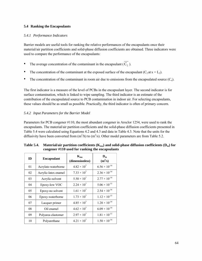
5.4 Ranking the Encapsulants

5.4.1 Performance Indicators

Barrier models are useful tools for ranking the relative performances of the encapsulants once their material/air partition coefficients and solid-phase diffusion coefficients are obtained. Three indicators were used to compare the performance of the encapsulants:

• The average concentration of the contaminant in the encapsulant ( C2 ).

• The concentration of the contaminant at the exposed surface of the encapsulant (C2 at x = L2).

• The concentration of the contaminant in room air due to emissions from the encapsulated source (Ca).

The first indicator is a measure of the level of PCBs in the encapsulant layer. The second indicator is for surface contamination, which is linked to wipe sampling. The third indicator is an estimate of the contribution of the encapsulated source to PCB contamination in indoor air. For selecting encapsulants, these values should be as small as possible. Practically, the third indicator is often of primary concern.

5.4.2 Input Parameters for the Barrier Model

Parameters for PCB congener #110, the most abundant congener in Aroclor 1254, were used to rank the encapsulants. The material/air partition coefficients and the solid-phase diffusion coefficients presented in Table 5.4 were calculated using Equations 4.2 and 4.3 and data in Table 4.3. Note that the units for the diffusivity have been converted from (m2/h) to (m2/s). Other model parameters are from Table 5.2.

Table 5.4. Material/air partition coefficients (Kma) and solid-phase diffusion coefficients (Dm) for congener #110 used for ranking the encapsulants

ID Encapsulant Kma

(dimensionless)

Dm

(m2/s)

01 Acrylate-waterborne 4.82 × 107 6.56 × 10-14

02 Acrylic-latex enamel 7.33 × 107 2.36 × 10-14

03 Acrylic-solvent 5.50 × 107 2.77 × 10-14

04 Epoxy-low VOC 2.24 × 107 5.06 × 10-15

05 Epoxy-no solvent 1.61 × 107 2.54 × 10-16

06 Epoxy-waterborne 1.73 × 107 1.12 × 10-15

07 Lacquer primer 4.85 × 107 1.28 × 10-14

08 Oil enamel 4.62 × 107 6.09 × 10-14

09 Polyurea elastomer 2.97 × 107 1.81 × 10-13

10 Polyurethane 4.21 × 107 1.50 × 10-14

64

A

vera

ge

C2

(µg

/g)

30

25

20

15

10

5

0

5.4.3 Ranking the Encapsulants Based on Absolute Concentrations

Figures 5.21 through 5.23 rank the ten encapsulants based on the three performance indicators described in Section 5.4.1. The rankings based on the second and third criteria are similar to the rankings from the experimental results, but the ranking based on the average concentration in the encapsulant showed a different pattern. As discussed in Section 5.3.2, the accumulation of contaminant in the encapsulant is controlled by two factors, i.e., the gain due to the contaminant flux from the source and the loss due to emissions to room air. Thus, a good encapsulant that significantly reduces the concentrations of PCBs at the exposed surface and in the indoor air does not necessarily perform well in lowering the average concentration in the encapsulant layer.

Figure 5.21. Ranking of encapsulants by the average concentration in the encapsulant layer (Average C2)

(For congener #110; t = 500 days; initial concentration in source = 100 µg/g)

65

C

2 (x

=L2)

(µ

g/g

) 25

20

15

10

5

0

0.5

Air

Co

nce

ntr

atio

n (µ

g/m

3 )

0.4

0.3

0.2

0.1

0

Figure 5.22. Ranking of encapsulants by the concentration at the exposed surface of the encapsulant layer [C2 (x=L2)]

(for congener #110; t = 500 days; initial concentration in source = 100 µg/g)

Figure 5.23. Ranking of encapsulants by the air concentration due to emissions from the encapsulated source

(For congener #110; t = 500 days; initial concentration in source = 100 µg/g)

66

5.4.4 Ranking the Encapsulants Based on Percent Reduction of Concentrations

Sometimes it is more useful to rank the encapsulants based on percent reduction of the PCB concentrations as compared to the not-encapsulated source. Figure 5.24 shows the concentration profiles of congener #110 in the not-encapsulated source (concrete). The average concentration in the top layer (0.1 mm thick) is 19.7 µg/g; the concentration at the exposed surface is 13.2 µg/g; the air concentration is 0.38 µg/m3. The percent reductions are shown in Tables 5.5 through 5.7. Overall, the epoxy coatings perform well in keeping the concentration low at the exposed surface and in the room. The acrylic coatings performed poorly.

As shown in Table 5.5, a good encapsulant, which effectively reduces the PCB concentration at the exposed surface and the contribution to air pollution, does not necessarily perform well in keeping the average concentration low in the encapsulant layer because a good encapsulant reduces the PCB loss due to emissions and, thus, facilitates the accumulation of PCBs in the encapsulant layer.

The results shown in Tables 5.5 through 5.7 also show that selecting the wrong encapsulant may make the contamination worse (i.e., negative percent reduction). A key factor that determines the distribution of PCBs between the source and encapsulant is the partition coefficient between the two phases. PCB molecules tend to migrate from the source to, and concentrate in, the encapsulant if the latter has a large material/air partition coefficient, which leads to a large material/material partition coefficient (Equation 4.4).

120

100

80

60

40

20

0

C 1 (

x)

(μg

/g)

0 1 2 3 4 5

x (mm)

Figure 5.24. Concentration profiles for congener #110 in not-encapsulated concrete at t = 500 days

(The blue dotted line separates the top layer (0.1 mm thick) from the rest of the source)

67

Table 5.5. Ranking the encapsulants by percent reduction of the average concentration in the top 0.1 mm of the layer, i.e., the thickness of the encapsulant (For congener #110; initial concentration in source = 100 µg/g; t = 500 days)

Encapsulant % Reduction Rank

Polyurea elastomer 50.7% 1

Epoxy-low VOC 33.3% 2

Oil enamel 21.3% 3

Polyurethane 18.4% 4

Acrylate-waterborne 18.2% 5

Epoxy-waterborne 15.7% 6

Epoxy-no solvent 7.8% 7

Lacquer primer 5.6% 8

Acrylic-solvent 2.7% 9

Acrylic-latex enamel -29.5% 10

Table 5.6. Ranking the encapsulants by percent reduction of the concentration at the exposed surface (For congener #110; initial concentration in source = 100 µg/g; t = 500 days)

Encapsulant % Reduction Rank

Epoxy-no solvent 96.1% 1

Epoxy-waterborne 84.5% 2

Epoxy-low VOC 55.2% 3

Polyurea elastomer 28.2% 4

Polyurethane 0.0% 5

Oil enamel -12.1% 6

Lacquer primer -15.4% 7

Acrylate-waterborne -17.1% 8

Acrylic-solvent -33.3% 9

Acrylic-latex enamel -79.2% 10

68

Table 5.7. Ranking the encapsulants by percent reduction of the concentration in room air (For congener #110; initial concentration in source = 100 µg/g; t = 500 days)

Encapsulant % Reduction Rank

Epoxy-no solvent 89.8% 1

Epoxy-waterborne 62.7% 2

Epoxy-low VOC 16.7% 3

Polyurethane 1.0% 4

Lacquer primer 0.8% 5

Polyurea elastomer -0.9% 6

Acrylic-solvent -1.1% 7

Oil enamel -1.2% 8

Acrylate-waterborne -1.3% 9

Acrylic-latex enamel -2.0% 10

5.5 Limitations of Mathematical Modeling

The simulation results presented above used the three performance indicators: the average concentration in the encapsulant layer, the concentration at the exposed surface of the encapsulant later, and the contribution of the encapsulated source to the concentration in air. They were used to better understand the general behavior of encapsulated sources and compare the relative performances of the encapsulants. These indicators are difficult to measure in the real-world situations.

The partition and diffusion coefficients used as the input of the barrier model were rough estimates. The average RSD was 35% for the partition coefficients and 55% for the diffusion coefficients.

The simulations were conducted by assuming that the PCB concentration in the source is uniform initially. In the real world, a concentration gradient may exist in many PCB-contaminated building materials.

Although the barrier model was developed based on mass transfer theories, its long term predictions have not been validated by experimental data. Thus, the simulation results presented above should be considered semi-quantitative and can only compare the relative performances of the encapsulants.

69

6. Discussion

6.1 Effectiveness and Limitations of the Encapsulation Method

The experimental data (Sections 4.1.2 and 4.2.4) and the results of mathematical modeling (Sections 5.4.3 and 5.4.4) showed that selecting high-performance encapsulants can effectively reduce the PCB concentrations in the encapsulant layer, at the exposed surfaces, and in indoor air. On the other hand, the encapsulation method has its limitations. As shown in Figure 4.9, when the source contained 13000 µg/g PCBs, the PCB concentrations in the wipe samples for the encapsulated panels ranged from 10.1 to 584 µg/100 cm2 depending on the encapsulant used. Thus, if the goal is to keep the PCB concentration in the wipe sample below 10 µg/100 cm2, only one encapsulant barely met the requirement.

Estimating the upper limit of the PCB concentration in the source for successful encapsulation is more difficult than it appears because several factors must be considered. These include selection of the performance criteria and safety factor, the properties of the encapsulant (e.g., the resistance to PCB migration and the thickness of the coating), and the properties of the source (e.g., partition coefficient). If the ultimate goal is to control the PCB concentration in room air, the area of the source and the environmental conditions (e.g., ventilation rate and the presence of other sources) should also be considered.

Depending on the mitigation goals, the performance criteria can be the PCB concentration in wipe samples, the average PCB concentration in the layer of the encapsulant, the PCB concentration at the exposed, encapsulated surface, and the contribution to the PCB concentration in room air. Among these criteria, wipe sampling is the easiest to implement. Use of other criteria relies heavily on mathematical modeling. It should be noted that the concentration in the wipe sample is closely related to, but not the same as, the concentration at the exposed surface because the solvent used for wipe sampling may penetrate into some substrates.

According to the results of mathematical modeling, the average concentration in the encapsulant, the concentration at the exposed surface, and the concentration in room air all showed linear relationships with the initial concentration in the source (Section 5.3.7). Such linear relationship should also apply to wipe samples because they are related to the concentrations at the exposed surface. Thus, the upper limit of the encapsulating ability of a coating material can be estimated from Equation 6.1:

C Wmax Cmax = (6.1) WS f

where Cmax = maximum allowable concentration of PCBs in the source for effective encapsulation (µg/g)

C = measured PCB concentration in the source where the wipe sample is taken (µg/g)

Wmax = mitigation goal expressed as the maximum allowable PCB concentration in wipe samples

(µg/100 cm2)

Sf = safety factor (dimensionless)

70

W = measured PCB concentration in the wipe sample for the encapsulated source (µg/100 cm2)

Among the four parameters on the right-side of the equation, C and W are either from experimental data or mathematical modeling, whereas Wmax and Sf are determined by the decision-makers or risk assessors. For example, for the wipe sampling tests described in Section 4.2, C ≈ 13000 µg/g (Table 4.4). If the Epoxy-no solvent is used as the encapsulant, then W = 10.1 µg/100 cm2 (Figure 4.9). For demonstration purposes, Wmax is set to 1 µg/100 cm2 and Sf to 3. Then Cmax can be calculated:

13000 ×1C = ≈ 430 (µg/g) (6.2) max 3 ×10.1

If Wmax is relaxed to 10 µg/100 cm2, then Cmax = 4300 (µg/g).

One factor that Equation 6.1 does not consider is the thickness of the encapsulant. In general, the thickness of the encapsulant used in the field should be comparable with or greater than the thickness of the encapsulant used in the laboratory testing from which parameters C and W are obtained.

As we demonstrated in Part 2 of this report series (Guo et al., 2012), the interior surfaces contaminated with PCBs due to sorption from room air, also known as PCB sinks or “secondary sources”, may become emitting sources after the primary sources are removed. Because of their large quantities, mitigating these “secondary sources” is difficult and costly. The encapsulation method has the potential to substantially reduce the cost by not having to remove the contaminated materials from the building.

A disadvantage of using wipe sampling as the performance criteria is that the PCB concentration in the wipe samples does not correlate to the concentration in room air because the latter is also dependent on the area of the source, the ventilation rate, and the presence of other PCB sources. As a practical matter, post-encapsulation monitoring (e.g., wipe and air sampling) is essential for successful encapsulation.

6.2 Selection of Encapsulants

Resistance to PCB migration is one of the key factors for selecting proper encapsulants for PCB sources. The results of both the sink tests (Section 4.1) and the wipe sampling tests (Section 4.2) showed that the performances of the ten coating materials were significantly different. Table 6.1 compares the performances of the ten encapsulants based on the maximum allowable PCB concentrations in the source (Cmax) for effective encapsulation. The results were calculated by using Equation 6.1 and the wipe sampling data presented in Figure 4.9.

Overall, the epoxy coatings performed better than the other types of coating materials because they were more effective in reducing the surface concentrations. The performance of the Polyurea elastomer should be re-evaluated in future studies because the sink tests and wipe sampling tests yielded difference results (Figures 4.7 versus Figure 4.9). As a general guideline, the coating materials that have smaller material/air partition coefficients and smaller diffusion coefficients perform better in reducing the concentrations of PCBs at the exposed surface and in the indoor air (Figures 5.22 and 5.23). An encapsulant that has a small material/air partition coefficient also has a small fugacity capacity, resulting in more resistance to PCB migration from the source. Similarly, an encapsulant that has a small diffusion coefficient impedes the

71

mobility of the PCB molecules, thereby creating a steep concentration gradient, which, in turn, helps reduce the PCB concentrations at the exposed surface.

Table 6.1. Calculated maximum allowable concentrations in the source for effective encapsulation ) [a] with two mitigation goals based on the PCB concentration in wipe samples (Wmax

Encapsulant

Maximum Allowable PCB Concentration

in the Source, Cmax, (µg/g) [b]

For Wmax = 1 µg/100 cm2 For Wmax = 10 µg/100 cm2

Lacquer primer 7.4 74

Acrylic-latex enamel 8.8 88

Oil enamel 14 140

Polyurethane 18 180

Acrylic-solvent 19 190

Acrylate-waterborne 19 190

Epoxy-waterborne 34 340

Polyurea elastomer 69 690

Epoxy-low VOC 120 1200

Epoxy-no solvent 430 4300 [a] See Table 3.10 for the accuracy of the wipe sample data. [b] Results are rounded to two significant digits.

There are many types of coating materials on the market that can potentially be used as encapsulants for PCB sources. Although the epoxy coatings performed well among the ten coating materials we tested, they may not be the best encapsulants available. The authors recommend that more types of coating materials be tested in future studies, including silicon-based coating materials. Polyurea elastomer should also be included because this study gave inconsistent results.

In practice, several more factors should be considered when selecting proper encapsulants, including elongation (i.e., elasticity or rigidity), dry-film thickness, hardness, drying or curing time, compatibility with existing surfaces, and ease of application (Mitchell and Scadden, 2001). Successful encapsulation also depends on other factors, such as surface preparation and post-encapsulation monitoring (EH&E, 2012).

6.3 Potential Effect of the Weathering of Encapsulants on their Encapsulating Ability

Polymeric materials are the bases of most coating materials. Environmental conditions may cause degradation, or weathering, of the polymeric materials. The major factors that contribute to material degradation include ultraviolet (UV) irradiation, moisture, elevated temperature, and temperature fluctuations. Although the accelerated aging tests described in Section 4.2.5 were not conclusive, no serious PCB breakthroughs were observed. Given that the intensity of UV irradiation is much weaker and the

72

temperature fluctuations are much smaller indoors than outdoors, the degradation of coating materials in the indoor environment is expected to be much slower than in the outdoor environment.

Because of the harsh conditions in the ambient environment, encapsulants applied to the exterior surfaces may deteriorate faster than those applied to the interior surfaces. Thus, post-encapsulation monitoring is even more important for encapsulating exterior surfaces. For future studies, the effect of weathering should be investigated by conducting the weathering tests under realistic or simulated outdoor environmental conditions. Such tests are time-consuming and costly, however.

Another factor to be considered to judge the performance of the encapsulation is the change of the PCB concentrations in the encapsulant layer over time. If the concentrations increase continuously over time, the protective effect of the encapsulation may eventually fail. However, the modeling results presented in Sections 5.3.3 and 5.3.4 suggests otherwise, i.e., the peak concentrations in the encapsulant layer occurred in a several weeks, followed by a decrease in concentrations over time due to the formation of a concentration gradient in the source.

6.4 Encapsulating Encapsulated Sources

The performance of an encapsulant may deteriorate over time due to environmental factors such as wearing and aging. Adding a new layer of encapsulant may improve the protective effect because of the added thickness (See Section 5.3.6) and coverage of damaged spots. When used in conjunction with the post-encapsulation monitoring plan, such practice may prolong the protective effect of the encapsulation.

6.5 Effectiveness of Encapsulating Sources with High PCB Content

This study demonstrated that, although some of coating materials we tested performed much better than others as PCB encapsulants, none of them is truly impenetrable to PCB molecules. Thus, as discussed above, coating materials alone may not be effective in meeting mitigation goals for sources that have a high PCB content. However, under certain circumstances, encapsulating sources with high levels of PCBs could still be beneficial. For example, there may be a substantial volume of caulking that is scheduled for removal at some mitigation sites. Developing and implementing a remediation plan requires proper planning and funding. In such cases, encapsulating the caulk may help reduce potential exposures during this time period. Using encapsulation under such circumstances must be considered as a short-term interim measure.

6.6 Relationship between the Sink Tests and the Wipe Sampling Tests

At first glance, the sink tests and wipe sampling tests are unrelated to each other because they are based on completely different mass transfer mechanisms. In fact, the two experimental methods are closely related because of Equation 6.3 (i.e., Equation 4.4):

Kma _1K12 = (6.3) Kma _ 2

where K12 = material/material coefficient between material 1 and material 2 (dimensionless) Kma_1 = material/air partition coefficient for material 1 (dimensionless)

73

Kma_2 = material/air partition coefficient for material 2 (dimensionless)

The material/air partition coefficient (Kma) is not only a key factor that determines the sorption concentration in the sink tests, it also determines the partition coefficient between the source and the encapsulant (Equation 6.3). Thus, an encapsulant with a small material/air partition coefficient (Kma_1) also has a small encapsulant/source partition coefficient (K12), which means a greater resistance to PCB migration from the source (material 2) to the encapsulant (material 1).

6.7 Study Limitations

This study was limited to laboratory testing with a limited scope. Only ten coating materials were tested. There are many coating materials that can potentially be used as PCB encapsulants. The test results of this study may not be applicable to the similar products that were not tested even within the same class of coatings. One coating material that is currently sold as a PCB encapsulant by a foreign manufacturer was not tested because of the authors’ inability to obtain the product for testing.

This study was narrowly focused on the effectiveness and limitations of the encapsulation method, the performances of a limited number of encapsulants, and the factors that may affect the performance of encapsulation. It is not a comprehensive evaluation of the encapsulation method.

The wipe sample data presented in Sections 4.3.4 and 4.3.5 did not meet all the data quality goals. The uncertainty of the data was between 25% and 50% as estimated based on the accuracy and the precision of the QC samples. Thus, the data must be considered as semi-quantitative.

The solid/air partition coefficients and solid-phase diffusion coefficients reported in Table 4.3 are rough estimates. More accurate measurements of these properties for encapsulants are needed because they are the key parameters that affect the performance of encapsulants. They are also the key input parameters for the barrier models. For more accurate measurements, the two parameters must be determined separately.

Wipe sampling is a simple and useful way to determine the PCB contamination at surfaces, including encapsulated surfaces. However, the correlation between the concentrations of PCBs in wipe samples and the concentrations in the solid material is poorly understood. For example, the difference in porosity of the surface materials may cause significant difference in the wipe sampling results. To use the wipe sampling method to monitor the performance of the encapsulants, standardization of the method, such as selection of the solvent, is needed. Hexane, the commonly used solvent for wipe sampling for PCBs, can destroy some of the coating materials, causing difficulty in sample analysis.

In Section 5.3, the general behavior of encapsulated sources was evaluated by using a barrier model. The simulations were made for congener #110, the most abundant congener in Aroclor 1254, with one set of input parameters. In real world settings, multiple congeners and multiple sets of environmental parameters should be considered.

74

75

7. Conclusions

Ten coating materials were tested for their performances as encapsulants for PCBs by using two experimental methods, i.e., sink tests and wipe sampling tests [Sections 2.1, 2.2 and 2.3]. In general, the results from the two types of tests yielded similar results. The performances of the encapsulants differed significantly. Selecting high-performance encapsulants is a key step. Overall, the three epoxy coatings performed better than the other coatings [Sections 4.1, 4.2, and 6.2]. An encapsulant with a smaller material/air partition coefficient and a smaller solid-phase diffusion coefficient performs better in reducing the PCB concentrations at the exposed surface and in indoor air [Sections 4.1.3, 5.3, and 6.2]. Increasing the thickness of encapsulant (e.g., applying multiple coats) helps reduce the PCB concentration at the exposed surface and, thus, reduce the contribution of the encapsulated source to the PCB concentration in indoor air. [Sections 4.2.6.1 and 5.3.6]

Encapsulation can be used as an interim solution to mitigating PCB contamination in buildings [Section 6.1]. It may not be effective in meeting mitigation goals for sources that contain high concentrations of PCBs such as PCB-containing caulking material because, for a given source and a given encapsulant, the concentration of PCBs in the encapsulant layer is proportional to the PCB concentration in the source and because none of the coating materials we tested was truly impenetrable to PCBs. [Sections 5.3.7 and 6.5]

Encapsulation is most effective for contaminated interior surfaces that have large areas and that contain low levels of PCBs. Because of their large quantities, mitigating these “secondary sources” is difficult and costly. The encapsulation method has the potential to substantially reduce the cost by not having to remove the contaminated materials from the building. [Section 6.1]

Barrier models are useful tools for studying the general behavior of encapsulated sources and ranking the performances of encapsulants. These models complement and supplement the experimental results by providing three criteria for evaluating encapsulants, i.e., (1) the average concentrations of PCBs in the encapsulant layer; (2) the concentrations of PCBs at the exposed surface of the encapsulated source; and (3) the contribution of the encapsulated source to the concentrations of PCBs in indoor air. In most cases, the second and third criteria are more stringent than the first criterion. The material/air partition coefficient and the solid-phase diffusion coefficient are two key parameters that link the experimental results to the barrier models. [Section 5]

Determination of the upper limit of the PCB concentration in the source for successful encapsulation depends on several factors including the mitigation goals, the properties of the source, the properties of the encapsulant, and the environmental conditions. A combination of experimental testing and mathematical modeling is the best approach to determining the limitations of the encapsulation method. Wipe sampling is the most common method for measuring surface contamination and can be used as a criterion for evaluating the performances of encapsulants [Sections 6.1 and 6.2].

Equation 6.1 can be used to estimate the maximum allowable concentration of PCBs in the source for effective encapsulation (Cmax). For example, based on the wipe sampling results presented in Section 4.2.4, Cmax is estimated to be 430 µg/g, assuming (1) the maximum allowable PCB concentration in the wipe

76

sample is 1 µg/100 cm2, (2) Epoxy-no solvent coating ― the most effective encapsulant we tested ― is used, and (3) the safety factor is 3. [Section 6.1]

Although the epoxy coatings performed well in this study, they may not be the best encapsulants available because many coating materials, including silicon-based coatings, were not tested [Sections 2.1, 6.2, and 6.7]. The two test methods described in this study [Sections 2.2 and 2.3] can be used to screen a wide range of coating materials.

The results from accelerated aging tests for encapsulated PCB sources were inconclusive. Because the intensity of the UV light is much weaker and the temperature is much stable indoors than outdoors, the deterioration of the encapsulant in the interior of the building due to weathering is expected to be much slower and, thus, the effective encapsulation for the interior of the building is expected to last longer than for the exterior of the building. In either case, post-encapsulation monitoring is essential. [Sections 4.2.5 and 6.3]

Building owners should be aware of the effectiveness and limitations of the encapsulation method and the factors that may affect the effectiveness of the method. Selecting high-performance coating material is a key to successful encapsulation of PCB-contaminated surfaces. A long-term monitoring plan is essential to ensure the integrity of the seal. [Sections 6.1 and 6.2]

77

8. Recommendations

This study is limited in scope. The authors recommend the following topics for future research.

1. Screen (e.g., by the wipe sampling method) a wide range of coating materials to determine their encapsulating abilities for PCBs. Candidate coating materials should include all those that have been used as the PCB encapsulants in the field and all those that are currently marketed as PCB encapsulants. Polyurea coatings should be included because this study gave inconsistent results.

2. Evaluate the performances of the encapsulants by using realistic source substrates such as masonry. A major difficulty in conducting such tests is to develop the sources in which the PCBs are uniformly distributed.

3. Evaluate the encapsulation methods that use more than one type of coatings, such as the use of a primer or a top coat over the encapsulant. The effectiveness and performance of non-liquid materials should also be investigated. For example, using solid films (such as flexible metallic tapes) that are impenetrable to PCBs may allow encapsulation of sources with higher PCB content.

4. Develop experimental methods that can evaluate the effects of weathering on the performance of the encapsulants. Data from such tests will help evaluate the effectiveness of encapsulating exterior walls.

5. Develop methods to determine the material/air partition coefficients and solid-phase diffusion coefficients for PCB congeners more accurately to reduce the uncertainty in the predictions by the barrier models. These parameters are also essential for using the source and sink models.

6. Develop an integrated modeling framework for PCBs in buildings to allow decision-makers, school managers, building owners, and practitioners to evaluate mitigation options, including the effect of encapsulation on indoor air quality, and to compare the effectiveness of the mitigation methods. Developing such a framework also sheds light on data gaps. In the past two decades, many mass transfer models have been developed for emissions from building materials, sorption by interior surfaces (i.e., the sink effect), and contaminant barriers. While these models are essential tools that have helped us better understand the movements of PCBs in buildings, none of them can handle the complex cases presented by the PCB contamination in buildings. For the framework to be useful to a broad range of users, it should allow for multiple sources and sinks in the room, including layered sources (e.g., encapsulated sources) and layered sinks (e.g., painted masonry walls). Other useful simulation capabilities include PCB migration from primary sources (e.g., caulk) to adjacent materials (e.g., masonry walls), removal of primary sources, use of stand-alone air cleaning devices, variable ventilation rate, and temperature changes.

78

Acknowledgments

The authors thank Drs. John Little and Zhe Liu of the Virginia Polytechnic Institute and State University for technical consultation on barrier models and for providing the MATLAB code for the barrier model used in this report; Jacqueline McQueen of EPA’s Office of Science Policy for assistance in communications; and Robert Wright of EPA’s National Risk Management Research Laboratory and Joan Bursey of EPA’s National Homeland Security Research Center for QA support.

79

References

(Website accessibilities were last verified on November 15, 2011)

ASTM (2004a). E1795-04 Standard specification for non-reinforced liquid coating encapsulation productsfor leaded paint in buildings. ASTM International, West Conshohocken, PA.

ASTM (2004b). E1797-04 Standard specification for reinforced liquid coating encapsulation products forleaded paint in buildings. ASTM International, West Conshohocken, PA.

ASTM (2010a). E1494-92(2010) Standard practice for encapsulants for spray- or trowel-applied friableasbestos-containing building materials. ASTM International, West Conshohocken, PA.

ASTM (2010b). ASTM D5116-10 Standard guide for small-scale environmental chamber determinations oforganic emissions from indoor materials/products. ASTM International, West Conshohocken, PA.

ASTM (2010c). ASTM D4060-10 Standard test method for abrasion resistance of organic coatings by thetaber abraser. ASTM International, West Conshohocken, PA.

ASTM (2011). E1796-03(2011)e1 Standard guide for selection and use of liquid coating encapsulationproducts for leaded paint in buildings. ASTM International, West Conshohocken, PA.

Brown, S. K. (1990). Development of test methods for assessing encapsulants for friable asbestos insulationproducts, Journal of Coatings Technology, 62(782): 35-40.

Brown, S. K., and Angelopoulos, M. (1991). Evaluation of erosion release and suppression of asbestos fiberfrom asbestos building products, American Industrial Hygiene Association Journal, 52(9): 363-371.

Esposito, M. P., Mccardle, J. L., Crone, A. H., Greber, J. S., Clark, R., Brown, S., Halowell, J. B., Langham,A., and Mclardish, C. D. (1987). Decontamination Techniques for Buildings, Structures and Equipment,Noyes Data Corporation, Park Ridge, NJ, 252 pp.

EH&E (2012). Literature review of mitigation methods for PCBs in buildings, prepared for U.S. EPA byEnvironmental Health & Engineering, Inc., Report EPA/600/R-12/034.

Fuller, R., Klonne, D., Rosenheck, L., Eberhart, D., Worgan, J., and Ross, J. (2001). Modified Californiaroller for measuring transferable residues on treated turfgrass, Bulletin of Environmental Contamination andToxicology, 67: 787–794.

Guo, Z., Liu, X., Krebs, K. A., Stinson, R. A., Nardin, J. A., Pope, R. H., Roache, N. F. (2011). Laboratorystudy of polychlorinated biphenyl (PCB) contamination and mitigation in buildings ─ Part 1. Emissionsfrom selected primary sources, EPA/600/R-11/156, U.S. EPA, Office of Research and Development,National Risk Management Research Laboratory, 127 pp.

80

Guo, Z., Liu, X., Krebs, K. A., Greenwell, D. J., Roache, N. F., Stinson, R. A., Nardin, J. A., and Pope, R. H. (2012). Laboratory study of polychlorinated biphenyl (PCB) contamination and mitigation in buildings ― Part 2. Transport from primary sources to building materials and settled dust, EPA/600/R-11/156a, U.S. EPA, Office of Research and Development, National Risk Management Research Laboratory, 166 pp.

Hu, H. P., Zhang, Y.P., Wang, X.K. , and Little, J. C. (2007). An analytical mass transfer model for predicting VOC emissions from multi-layered building materials with convective surfaces on both sides, International Journal of Heat and Mass Transfer, 50: 2069–2077.

Kumar, D. and Little, J. C. (2003). Characterizing the source/sink behavior of double-layer building materials, Atmospheric Environment, 37: 5529–5537.

Little, J. C., Kumar, D., Cox, S. S., and Hodgson, A. T. (2002). Barrier materials to reduce contaminant emissions from structural insulated panels. Advances in Building Technology, Anson, M., Ko, J. M., and Lam, E. S. S. (eds.), Elsevier Science Ltd., Vol. 1, pp 113-120.

Mackay, D. and Paterson, S. (1981). Calculating fugacity. Environmental Science & Engineering, 15(9): 1006-1014.

Mackay, D. and Paterson, S. (1982). Fugacity revisited. Environmental Science & Engineering, 16(12): 654A-660A.

Martyny, J. W. (2008). Encapsulation of methamphetamine-contaminated building materials, National Jewish Medical and Research Center. http://health.utah.gov/meth/html/Decontamination/AdditionalResources.html

MIC (undated). PCB encapsulation. Midwest Industrial Coatings-WI, LLC. http://www.midwestindustrialcoatings.com/pcb.html

Mitchell, S. J. and Scadden, R. A. (2001). PCB decontamination methods for achieving TSCA compliance during facility decommissioning projects. The National Defense Industrial Association Annual Environmental Symposium, Austin, Texas, 25 April 2001, Technical Paper 0102. http://www.westonsolutions.com/about/news_pubs/tech_papers/MitchellNDIA01.pdf

NERL (2010). A Research Study to Investigate PCBs in School Buildings, EPA 600R-10/074, National Exposure Research Laboratory. http://www.epa.gov/pcbsincaulk/research-plan.pdf

Pizarro, G. E. L., Dzomak, D. A., and Smith, J. R. (2002). Evaluation of cleaning and coating techniques for PCB-contaminated concrete. Environmental Progress, 21(1): 47-56.

Robnor Resins (Undated). Robnor Polyurethane Applications. http://www.robnor.co.uk/index.php/products/polyurethane.html

81

Scadden, R. A. and Mitchell, S. J. (2001). A case study of the continued use of PCB-contaminated concrete through implementation of the 40 CFR 76130(p) use authorization, 10th Annual RCS, National Convention, Austin, TX, October 2001. Technical Paper #0204. http://www.westonsolutions.com/about/news_pubs/tech_papers/ScaddenRCS2001.pdf

TWO Teknik (2011). TWO SCI - Silicon PCB Stop (SPS). http://www.twoteknik.dk/index.php?content=page&id=47

U.S. EPA (2007). EPA Method 8082A, Polychlorinated biphenyls (PCBs) by gas chromatography. http://www.epa.gov/waste/hazard/testmethods/sw846/pdfs/8082a.pdf

U.S. EPA (2008a). EPA Method 1668B, Chlorinated biphenyl congeners in water, soil, sediment, biosolids and tissue by high resolution gas chromatography/high resolution mass spectrometry (HRGC/HRMS). http://epa.gov/waterscience/methods/method/files/1668.pdf

U.S. EPA (2008b). Test methods for evaluating solid waste, physical/chemical methods, in EPA publication SW-846, U.S. EPA, Government Printing Office, Washington, D.C.

Willett, L. B. (1972). Barrier coatings to prevent polychlorinated biphenyl (PCB) contamination of silage. Ohio Agricultural Research and Development Center Research Summary, 59: 28-32.

Willett, L. B. (1973). The evaluation of barrier coatings in farm silos which were PCB-contaminated. Ohio Agricultural Research and Development Center Research Summary, 69: 36-39.

Willett, L. B. (1974). Coatings as barriers to prevent polychlorinated biphenyl contamination of silage. Journal of Dairy Science, 57(7): 816-825.

Willett, L. B. (1976). Coatings form effective barriers in PCB -contaminated silos. Ohio Report on Research and Development in Agriculture, Home Economics, and Natural Resources. 61(1): 5-6.

Yuan, H. Little, J. C., Marand, E., and Liu, Z. (2007). Using fugacity to predict volatile emissions from layered materials with a clay/polymer diffusion barrier. Atmospheric Environment, 41: 9300–9308.

82

Appendix A. Evaluation of the Wipe Sampling Method

A.1 Purpose

As described in Section 2.4.3, the wipe sampling method used in this study was developed based on a modified California roller method. This method requires placing a piece of aluminum foil between the wipe and roller. The potential loss of PCBs due to the use of the aluminum foil must be evaluated.

Hexane is the most widely used solvent for wipe sampling for PCBs. However, hexane was not suitable for this study because this solvent may destroy some painted surfaces, so we used 2-propanol instead. To make certain that 2-propanol had adequate collection efficiency for PCBs, side-by-side comparisons were made for the two solvents.

A.2 Method

The PCB source was created by mixing tetrachloro-m-xylene (TCMX, 0.00134% by weight), a commonly used surrogate compound for PCBs, with an alkyd primer. Ten aluminum panels were painted with the PCB primer. The area of the source was 60 cm2. After the primer was cured, wipe samples were taken by the roller method described in Section 2.4.3 with hexane and 2-propanol as the solvents. For each sampling event, the aluminum foil was extracted separately.

A.3 Results

A.3.1 Effect of Using Aluminum Foil

As shown in Table A.1, of the total TCMX collected by the sampling method, the aluminum foil contained less than 1% TCMX for 2-propanol and less than 3% TCMX for hexane.

Table A.1 Effect of using aluminum foil on wipe sampling

Solvent TCMX in wipe (ng)

TCMX in aluminum foil

Amount (ng) Fraction of total

2-Propanol

980 6.43 0.7% 1064 8.04 0.7% 852 3.92 0.5%

1097 5.94 0.5% 852 1.88 0.2%

Hexane

1097 27.8 2.5% 1068 23.4 2.1% 732 18.3 2.4%

1071 28.2 2.6% 1204 17.3 1.4%

83

A.3.2 Comparison of Solvents

Using the TCMX concentrations in the wipe samples presented in Table A.1, the statistics for the two solvents were calculated (Table A.2). The t-test yielded a two-tailed p value of 0.519, which means that the difference between these two solvents is not statistically significant.

Table A.2. TCMX concentrations in wipe samples: comparison of two solvents [a]

Statistics Solvent Mean SD n RSD 2) 2)(µg/100 cm (µg/100 cm

2- propanol 5 1.65 0.20 12.0%

Hexane 5 1.76 0.30 17.3% [a] The wiped area was 59 cm2.

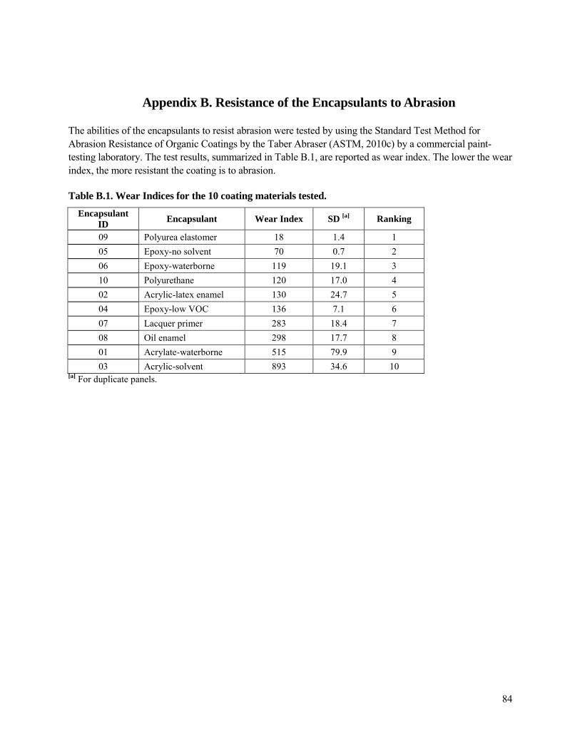
84

Appendix B. Resistance of the Encapsulants to Abrasion

The abilities of the encapsulants to resist abrasion were tested by using the Standard Test Method for Abrasion Resistance of Organic Coatings by the Taber Abraser (ASTM, 2010c) by a commercial paint-testing laboratory. The test results, summarized in Table B.1, are reported as wear index. The lower the wear index, the more resistant the coating is to abrasion.

Table B.1. Wear Indices for the 10 coating materials tested.

Encapsulant ID

Encapsulant Wear Index SD [a] Ranking

09 Polyurea elastomer 18 1.4 1 05 Epoxy-no solvent 70 0.7 2 06 Epoxy-waterborne 119 19.1 3 10 Polyurethane 120 17.0 4 02 Acrylic-latex enamel 130 24.7 5 04 Epoxy-low VOC 136 7.1 6 07 Lacquer primer 283 18.4 7 08 Oil enamel 298 17.7 8 01 Acrylate-waterborne 515 79.9 9 03 Acrylic-solvent 893 34.6 10

[a] For duplicate panels.