LABORATORY STUDY EVALUATING THERMAL REMEDIATION OF ...

LABORATORY STUDY EVALUATING THERMAL REMEDIATION

OF TETRACHLOROETHYLENE IMPACTED SOIL

by

JULIE MARIE BURGHARDT

A thesis submitted to the Department of Civil Engineering

in conformity with the requirements for the degree of

Master of Science (Engineering)

Queen’s University

Kingston, Ontario, Canada

December, 2007

Copyright © Julie Marie Burghardt

i

Abstract A laboratory study was conducted to assess the relationship between degree of volatile

organic compound (VOC) mass removal from soil and heating duration, initial dense non-

aqueous phase liquid (DNAPL) saturation, and grain size. The relationship between post-

remedy sampling temperature and VOC soil concentration was examined. Soil contained

in glass jars was spiked with DNAPL phase tetrachloroethylene (PCE), saturated, and

placed in an oven for a specified period of time. The soil temperature at the centre of each

jar was monitored during heating. Upon removal from the oven, each jar was immediately

capped with an air tight seal and placed into an ice bath until the soil temperature had

cooled to the desired sampling temperature. The jar caps were subsequently removed and

the soil was sampled using a coring tool and immersed into pre-weighed vials containing

methanol. PCE in soil samples was quantified using purge-and-trap with gas

chromatography/mass spectrometry.

Soil temperature increased steadily from ambient until reaching a plateau at 89 ºC ± 4 ºC

due to co-boiling of DNAPL phase PCE and water. A linear relationship was found

between the length of the co-boiling plateau and the initial PCE saturation. Co-boiling

continued until DNAPL phase PCE had been depleted, at which time the soil temperature

increased to the boiling point of water and remained constant while remaining pore water

was removed.

ii

PCE soil concentrations decreased rapidly in the early stages of heating, but leveled off

between 9.0 and 19 ppb soon after the soil became dried out. Analysis of the sensitivity to

initial PCE saturation data revealed that the concentration of PCE in post-remedy samples

increased with increasing initial saturation. Results of the sensitivity to grain size tests

showed a decreasing trend between PCE soil concentration and decreasing sand grain size

while temperature at sampling was not found to affect the amount of PCE quantified post-

thermal remedy.

Soil temperature at the centre of each jar during cooling was measured and an analytical

solution was fit to the recorded data. From this data, the thermal diffusivity of the soil

was approximated and was found to range from 1.4 x 10-7 to 1.8 x 10-7 m2/s.

iii

Acknowledgements

This research project was supported by Queen’s University through student scholarships

to the author.

I would like to express immense appreciation to my supervisor, Dr. Bernard Kueper, for

allowing me the opportunity to work on this challenging research project from which I

have gained copious knowledge and experience. Your expertise, advice, and words of

encouragement have been immeasurably valuable. The technical support provided by

Stan Prunster, Paul Thrasher, and Neil Porter is gratefully recognized. The assistance of

Dr. Allison Rutter, Paula Whitley, and fellow student Rebecca McWatters at the Queen’s

University Analytical Services Unit was essential for development of the analytical

method. Special thanks to Dr. Pat Oosthuizen from the Department of Mechanical

Engineering for lending his time to answer an abundance of questions over the course of

this project. In addition, the support of Fiona Froats, Maxine Wilson, and Cathy Wagner

is greatly appreciated.

Many thanks are directed to both the past and present members of the groundwater

research group, especially Keely Mundle, Sasha Richards, Grace Yungwirth, Brenda

Cooke, Mike West, Titia Praamsma, Dan Baston, and Eric Martin for their endless

support, inspiration, and wealth of knowledge. I am indebted to Erin Clyde, Indra

Kalinovich, Jennifer Littlejohns, Zoryana Salo, and Amanda Farquharson for their

reassurance, encouragement, and friendship.

iv

I wish to express profound gratitude to my parents and brother whose loving support and

encouragement has never been lacking. Your guidance, love, and confidence in me have

been immensely appreciated. Finally, special thanks to Matthew without whose support

and reassurance, this thesis would not have been completed.

v

Forward

This thesis has been written in manuscript form, such that a Chapter 1 provides a general

introduction, Chapter 2 presents a review of relevant literature, and Chapter 3 is a

complete independent manuscript that will be submitted for publication. Julie Burghardt

is the lead author of the manuscript. Concluding remarks and recommendations are

presented in Chapter 4. Supplemental experimental data and calculations, information on

the analytical method and analytical error, details regarding the mathematical model, and

information on the properties of tetrachloroethylene as a function of temperature are

provided in Appendices A through E.

vi

Contents

Abstract i

Acknowledgements iii

Forward v

Contents vi

List of Tables x

List of Figures xi

Nomenclature xiv

Abbreviations xix

Chapter 1 – Introduction 1

1.1 Research Objectives 6

1.2 Literature Cited 7

Chapter 2 – Literature Review 9

2.1 Fundamentals 9

2.1.1 Internal and Thermal Energy 9

2.1.2 Temperature 10

2.1.3 Heat and Thermal Equilibrium 11

2.2 Conduction 11

2.2.1 Thermal Conductivity 13

2.2.2 Specific Heat Capacity 14

2.2.3 Thermal Diffusivity 14

2.2.4 Heat Diffusion Equation 15

vii

2.3 Convection 16

2.3.1 Governing Equations 19

2.3.2 Phase Change Convection 21

2.4 Radiation 22

2.4.1 Surface Emission 22

2.4.2 Radiation Exchange 24

2.5 Heat Transfer in Soil 26

2.5.1 Porosity 26

2.5.2 Heat Transfer Mechanisms in Soil 27

2.5.3 Conduction in Porous Media 28

2.5.4 Effective Thermal Conductivity 28

2.5.5 Convection in Porous Media 29

2.5.6 Boiling in Soil 31

2.6 Thermal Properties of Soil and Rock 33

2.6.1 Dependence on Porosity and Saturation 35

2.6.2 Dependence on Mineral Composition 38

2.6.3 Dependence on Grain Size 39

2.6.4 Dependence on Temperature 39

2.6.5 Dependence on Pressure 40

2.7 Thermal Remediation 42

2.7.1 Mechanisms for Contaminant Removal 43

2.7.2 Electrical Resistive Heating 51

2.7.3 Thermal Conductive Heating 52

viii

2.7.4 Steam Enhanced Extraction 53

2.7.5 Laboratory Studies 55

2.8 Post-Remedy Sampling Techniques for VOC Analysis 57

2.8.1 Hot Soil Sampling 60


Chapter 3 – Laboratory Study Evaluating Thermal Remediation of Tetrachloroethylene Impacted Soil 68

Abstract 68

3.1 Introduction 69

3.2 Materials 73

3.3 Methodology 76

3.3.1 Soil Heating Experiments 76

3.3.2 Mathematical Model 83

3.4 Results and Discussion 85

3.4.1 Soil Temperature During Heating 85

3.4.2 Sensitivity to Heating Time 88

3.4.3 Sensitivity to Initial PCE Saturation 90

3.4.4 Sensitivity to Grain Size 91

3.4.5 Sensitivity to Temperature at Sampling 93

3.4.6 Effect of Temperature on the Equilibrium Partitioning of PCE 95 3.4.7 Mathematical Model 98

3.5 Conclusions 102


ix

Chapter 4 – Conclusions and Recommendations 107

4.1 Conclusions 107

4.2 Recommendations 109

Appendices 111

x

List of Tables 1-1 Physical and chemical properties of common chlorinated solvents in relation

to water (adapted from Davis, 1997; a Crowe et al., 2001). 2 2-1 Thermal Properties of Some Common Soil and Rock Types. Values from

Schön, 2004 except: 1 Cermak and Rybach, 1982, 2 Adapted from Jumikis, 1977, 3 Bejan and Kraus, 2003, 4 U.S. Dept. of Defense, 2006. 35

2-2 Boiling points and co-distillation temperature of some common DNAPLs

(adapted form USEPA, 2004). 47 3-1 Mineralogy of composite and coarse sand samples. 76 3-2 Masses of each grain size in composite sand mixture. 78 3-3 Summary of experimental testing program. 81 3-4 Results for sensitivity to heating time laboratory tests (H1 to H5) and

base case test (B1). 89 3-5 Results from sensitivity to initial PCE saturation test (S1 to S4) and

base case. 91 3-6 Results of sensitivity to grain size experiments. 92 3-7 Results of sensitivity to temperature at sampling tests. 94

xi

List of Figures

1-1 Distribution of DNAPL in the subsurface following a surface release (adapted from Kueper et al., 2003). 3

2-1 Differential control volume in a) cartesian and b) cylindrical coordinates

(reproduced from Holman, 1997). 12 2-2 Thermal conductivities of a variety of materials (reproduced from

Incropera and DeWitt, 2002). 14 2.3 Elements of convective heat transfer (reproduced from Oosthuizen and

Naylor, 1999). 17 2.4 Convective velocity and temperature boundary layer distributions, where

u(y) and T(y) are the velocity and temperature distributions along the y-axis. (reproduced and adapted from Incropera and DeWitt, 2002). 18

2-5 Radiative cooling of a solid (reproduced and adapted from Incropera and

DeWitt, 2002). 24 2-6 Example of a porous medium (reproduced from Oosthuizen and

Naylor, 1999). 26 2-7 Velocity distribution across a vertical plane in a porous medium (reproduced

from Oosthuizen and Naylor, 1998). 30 2-8 Vapor, two-phase, and liquid zones with corresponding temperature profile

during boiling in porous media (adapted from Udell, 1985). 32 2-9 Direction of heat flux relative to the vertical (x) direction. 33 2-10 Thermal conductivities of common pore filling materials and minerals

(reproduced and adapted from Schön, 2004). 36 2-11 Thermal conductivity vs. porosity for sandstone and sand saturated

with water, oil and air (reproduced from Schön, 2004 - after Woodside and Messmer, 1961b). 37

2-12 Thermal conductivity vs. pressure for a gneiss rock sample (reproduced from

Schön, 2004). 41 2-13 Vapor pressure vs. temperature for common groundwater contaminants

(reproduced from Stegemeier and Vinegar, 2001). 44

xii

2-14 Boiling point of an ideal, miscible solution as a function of the composition of

the liquid (mole fraction of the components in the solution) (reproduced from Oxtoby et al., 1999). 45

2-15 Vapor pressures of PCE, water, and PCE-water immiscible mixture as a

function of increasing temperature (reproduced and adapted from Costanza, 2005). 47

2-16 Schematic representation of ERH system setup (adapted from USEPA,

2004). 52 2-17 Heater/Heater-Vacuum well configuration (Stegemeier and

Vinegar, 2001). 53 2- 18 Schematic representation of a steam enhanced extraction (SEE) process

(Davis, 1998). 54 3-1 Grain size curves for core segments 1, 2, 3, and 4. 74 3-2 Mean fraction organic carbon of sand samples of varying grain size. 75 3-3 Jar cap with thermocouple probe fitted through centre for measuring

temperature during cooling. 79 3-4 Schematic representation of laboratory setup for soil heating

experiments. 79 3-5 Finite cylinder used as approximation for soil filled jar in analytical model

(adapted from Luikov, 1968). 85 3-6 Soil temperature (± 4 °C) at jar center during oven heating experiment

for base case test (B1). 86 3-7 Length of co-boiling plateau in minutes as a function of initial

PCE saturation. 87 3-8 Concentration of PCE in soil samples as a function of heating time,

based on time before or after soil dry out. 89 3-9 Effect of initial PCE saturation (percent of pore space) on PCE quantified in

post thermally treated soil samples. 91 3-10 Post-thermal remedy soil PCE concentrations (individual samples and test

averages) as a function of sand grain size. 93

xiii

3-11 Effect of cooling (i.e. soil temperature at sampling ± 4°C) on the amount of PCE quantified in soil samples (individual samples and test averages). 95

3-12 Percentage of PCE mass in aqueous, gas, sorbed, and gas phases and

maximum PCE concentration without the presence of NAPL (CT) at varying temperature. 98

3-13 Soil temperature (± 4 °C ) at jar centre during cooling from experimental data and as derived by analytical model. 99

3-14 Temperature ( ± 4 °C) at jar centre during cooling in ice bath for test

H1 and H2, as compared with temperature profiles generated by analytical model. 101

Nomenclature

α thermal diffusivity (m2/s)

ε emissivity ([-])

Θ angle (rad)

λ wavelength (µm)

µ dynamic viscosity (Pa·s)

µn nth root of the Bessel function

ν wave frequency (Hz)

ρ density (g/cm3)

ρb soil dry bulk density (g/cm3)

ρf density of fluid (g/cm3)

ρPCE density of PCE (g/cm )3

ρs density of solid phase (g/cm3)

ρsg density of sand grains (g/cm3)

σ Stefan-Boltzmann constant = 5.67e-8 W/m2·K4

2sσ variance of the S statistic ([-])

φ porosity ([-])

φ w water porosity ([-])

φ a air porosity ([-])

Ф dissipation function (s-2)

Φl,v fluid potential (J/kg)

A area (m2)

xiv

xv

Aex peak area of experimental sample

Astnd peak area of standard

C specific heat capacity (J/kg·K)

Cex concentration of experimental samples (ppb)

Cg gas phase concentration (mg/L)

Cp specific heat capacity at constant pressure (J/kg·K)

Cpf specific heat capacity of fluid phase at constant pressure (J/kg·K)

Cps specific heat capacity of solid phase at constant pressure (J/kg·K)

Cstnd concentration of standard (ppb)

CT total soil concentration (mg/kg)

Cv specific heat capacity at constant volume (J/kg·K)

Cw aqueous phase concentration (mg/L)

c speed of light in a vacuum = 2.998x108 m/s

Eb emissive power of a blackbody (W/m2)

F12 view factor between surfaces 1 and 2 ([-])

Fo Fourier Number ([-])

foc fraction organic carbon ([-])

f fluid phase

g gravitational acceleration = 9.807 m/s2

H dimensionless Henry’s constant ([-])

H0 null hypothesis

HR dimensionless Henry’s constant at reference temperature ([-])

∆Hvap heat of vaporization (cal/mol)

∆HvapBP heat of vaporization at boiling point (cal/mol)

h convective heat transfer coefficient (W/m2·K)

hfg latent heat of vaporization (J/kg)

K permeability of porous media ([-])

Kd distribution coefficient (ml/g)

Koc organic carbon partitioning coefficient (ml/g)

Krl relative permeability of porous media to liquid phase ([-])

Krv relative permeability of porous media to vapor phase ([-])

k thermal conductivity (W/m·K)

ka apparent thermal conductivity (W/m·K)

kd dispersion conductivity (W/m·K )

ke effective thermal conductivity (W/m·K)

kf thermal conductivity of fluid phase (W/m·K)

ks thermal conductivity of solid phase (W/m·K)

l liquid

Mg mass in gas phase (mg/L)

MPCE mass of PCE (g)

Ms mass of soil (g)

Msb mass in sorbed phase (mg/L)

Mw mass in aqueous phase (mg/L)

m& l mass flux of liquid (kg/m2s)

m& v mass flux of vapor (kg/m2s)

nn moles of component n in gas phase (mol)

xvi

Pc capillary pressure (Pa)

Pl pressure of liquid (Pa)

Pn vapor pressure of component n (Pa)

Pn° pure component vapor pressure of n

Pt total pressure of a gas mixture (Pa)

Pv pressure of vapor (Pa)

Q heat transfer rate (W)

q heat flux (W/m2)

q& rate of energy generation per unit volume (W/m3)

qrad net radiative flux (W/m2)

R universal gas constant = 8.2057 × 10-5 atm·m3/mol·K

R2 coefficient of determination

RC universal gas constant = 1.9872 cal/mol·K)

r radius (m)

r, φ , z cylindrical coordinates

S solubility (mg/L)

SNW non-wetting phase (PCE) saturation (%)

s solid phase

sd standard deviation

sd2 sample variance

T temperature of porous media under assumption of LTE (ºC)

T∞ bulk fluid temperature (ºC)

T0 initial temperature (ºC)

xvii

Tb boiling point (ºC)

TC critical temperature (ºC)

Tf temperature of fluid (ºC)

TR reference soil temperature (ºC)

Ts temperature of solid surface (ºC)

Tsat saturation temperature (ºC)

Tsur temperature of surroundings (ºC)

t time (s)

ts Student’s t-value

u fluid velocity (m/s)

u∞ free stream fluid velocity outside boundary layer (m/s)

u, v, w velocity components in x, y, z directions, respectively (m/s)

V total volume (ml)

VJ volume of the jar (ml)

Vps volume of pore space (ml)

v vapor

wt % percent of total weight (%)

X1 mole fraction of component 1 in liquid phase ([-])

x sample mean

x, y, z rectangular coordinates

Y1 mole fraction of component 1 in gas phase ([-])

Z0 test statistic

xviii

xix

Abbreviations

ASTM American Society for Testing and Materials

bgs below ground surface

BTEX benzene, toluene, ethylbenzene, xylenes

CV coefficient of variation

DCE dichloroethylene

DCM dichloromethane

DNAPL dense non-aqueous phase liquid

EPA (USEPA) United States Environmental Protection Agency

ERH electrical resistive heating

GC-MS gas chromatography-mass spectrometry

HCL hydrochloric acid

LC34 launch complex 34

LNAPL light non-aqueous phase liquid

LTE local thermal equilibrium

MCL maximum contaminant level

MDL method detection limit

MGP manufactured gas plant

P&T purge-and-trap

PAHs polynuclear aromatic hydrocarbons

PCBs polychlorinated biphenyls

PCE tetrachloroethylene/perchloroethylene

xx

PTFE polytetrafluoroethylene

PVC polyvinylchloride

REV representative elementary volume

SEE steam enhanced extraction

SVE soil vapor extraction

SVOC semi-volatile organic compound

TCA trichloroethane

TCE trichloroethylene

TCH thermal conductive heating

VOA volatile organic analysis

VOC volatile organic compound

XRD x-ray powder diffraction

1

Chapter 1

INTRODUCTION

Chlorinated organic solvents such as tetrachloroethylene (PCE), trichloroethylene (TCE),

1,1,1-trichloroethane (TCA), and dichloromethane (DCM) are among the most

problematic sources of groundwater contamination in industrialized countries.

Production of these chemicals in the United States alone is in the hundreds of millions of

kilograms per year (Pankow and Cherry, 1996). Their uses range from chemical

intermediates to dry cleaning solvents, metal cleaning/degreasing, and, electronic and

pharmaceutical production. Most chlorinated solvents enter the subsurface through

leaking pipes, storage tanks, discharges from vapor degreasers, by past storage/disposal

directly onto land or unlined evaporation ponds, or by spills and leaks during

transportation (Kueper et al., 2003). Many chlorinated solvents have been found to affect

the central nervous system, are suspected or known carcinogens or mutagens, and/or have

been shown to cause liver or kidney damage in humans and animals (ATSDR, 2007a;

USEPA, 2006a; ATSDR, 2007b). Present in organic liquid form, chlorinated solvents are

denser than water and, as such, are referred to as “dense non-aqueous phase liquids” or

DNAPLs. Other DNAPLs include polychlorinated biphenyls (PCBs), creosotes, and coal

tars. Relevant physical and chemical properties of common chlorinated solvents are

presented and compared with water in Table 1-1.

Table 1-1: Physical and chemical properties of common chlorinated solvents in relation to water (adapted from Davis, 1997; a Crowe et al., 2001).

Compound

Boling Point (°C)

Density @ 25 °C

(g/cm3)

Viscosity @ 25 °C

(cP) Henry's

Constant [ - ]

Aqueous Solubility @ 20 °C (mg/L)

Tetrachloroethylene 121.3 1.613 0.844 0.928 ± 0.161 150

Trichloroethylene 87.3 1.4578 0.545 0.387, 0.38,

0.372 1100 1,1,1-

Trichloroethane 74.1 1.3303 0.793 1.13 ± 0.016 4400 Dichloromethane 40 1.3182 0.413 0.105 ± 0.008 20000

Water 100 0.997a 0.891a

DNAPLs are not totally immiscible in water, but have very low solubilities.

Consequently, they can be present in the subsurface as either a separate organic liquid

phase, or dissolved in water. As they are denser than water, DNAPLs have the ability to

penetrate the water table and move deeply through unconsolidated porous media and into

bedrock. Following a release, DNAPL will penetrate the subsurface both vertically and

laterally leaving behind disconnected blobs and ganglia of residual liquid and forming

pools of continuous liquid (Figure 1-1). A pool forms when DNAPL comes to rest on a

layer of fine grained material that acts as a capillary barrier. DNAPL will continue to

accumulate in a pool until the height of the pool produces a capillary pressure that

exceeds the entry pressure for the layer on which it rests, or until it spreads far enough

laterally to reach the edge of the layer. The DNAPL contained in a pool is continuous

through interconnected pore spaces, while residual DNAPL is disconnected.

2

Figure 1-1: Distribution of DNAPL in the subsurface following a surface release (adapted from Kueper et al., 2003).

Residual and pooled DNAPL will dissolve slowly into flowing groundwater forming

aqueous phase plumes that extend down gradient from the source zone. Complete

depletion of residual DNAPL by natural processes such as dissolution can take decades

(Kueper et al., 2003). Dissolution of the same mass of DNAPL, present in pooled form,

will occur at an even slower rate. Based on the solubility limit alone, a contaminant such

as PCE, with a moderately low solubility, can theoretically contaminate as much as

10,000 times its own volume, and, often observed contaminant concentrations are more

than a factor of 10 lower than the solubility limits, therefore, even small spills can

become substantial sources of contamination (MacKay et al., 1985).

Even though chlorinated solvents show low solubility in water, these solubility values are

high in relation to concentrations that are considered harmful to human health and the

3

4

environment. For example, the solubility of tetrachloroethylene (PCE) is 150 mg/L,

while The United States Environmental Protection Agency (USEPA) has set the drinking

water maximum contaminant level (MCL) for PCE at 5 µg/L, 30,000 times lower than the

contaminant’s solubility (USEPA, 2006a). The solubility of TCE is 1100 mg/L, while the

Ontario Ministry of the Environment, through the Environmental Protection Act, has

established the maximum allowable concentration of TCE in groundwater between 20

and 50 µg/L (Ontario Ministry of the Environment, 2004).

Chlorinated solvents belong to a class of chemicals known as volatile organic compounds

(VOCs), which are characterized by high vapor pressures and low solubility in water.

High vapor pressures and volatilities mean than chlorinated solvent gases can easily

diffuse into air filled pores of the unsaturated zone. Sampling of soils contaminated with

VOCs is often more difficult than sampling for non-volatile compounds, as a large

percentage of theses chemicals may equilibrate into the gas phase.

As remediation of sites contaminated with DNAPLs continues to be a priority in many

countries, much research has been conducted into improving the efficiency and

effectiveness of remediation technologies. In-situ thermal remediation techniques such as

steam flushing, electrical resistive heating, and thermal conductive heating have recently

been receiving increased attention due to their ability to overcome the mass transfer

limitations associated with traditional techniques such as pump-and-treat and soil vapor

extraction (SVE). Thermal remediation techniques involve heating the subsurface in

order to alter the physical and chemical properties of the contaminants and groundwater

5

to favor mobility. The primary mechanisms of contaminant removal are vaporization,

steam distillation, and boiling. Increasing the temperature of chlorinated solvents also

causes decreases in density, viscosity, and adsorption/absorption to soil matter, and

increases the rate of molecular diffusion in the liquid and gas phases (Davis, 1997).

Customary thermal remediation performance assessment involves sampling subsurface

material before and after the remediation process and determining through concentration

analysis if the post-operational concentration is within acceptable limits, or if the target

percentage mass removal has been met. Contaminant mass reductions in excess of 87 -

99 % have been reported by a number of authors (e.g., Beyke and Fleming, 2005; Heron

et al., 2005; Stegemeier and Vinegar, 2001), although some concerns have recently been

raised over the validity of this type of post treatment evaluation where the contaminants

of concern are VOCs. Elevated soil temperatures present post-thermal remedy increase

the vapor pressure of contaminants, resulting in increased volatilization and the

possibility of negative biases during post-remedy sampling.

Although a number of field and pilot studies have investigated the use of thermal

remediation techniques for DNAPL removal (e.g. Heron et al., 1998, and Hansen et al,

1998), very few laboratory experiments have been conducted to support these findings.

Even fewer studies have examined the effect of soil temperature on post-remedy

assessment.

6

1.1 Research Objectives

The primary objective of this work is to simulate the thermal remediation of PCE

contaminated soil in a laboratory setting and to determine the influence of various

parameters on post-heating soil concentration. Clean soil is impacted with PCE, placed

into glass jars, saturated with water, and heated in a convection oven. The sensitivity of

PCE soil concentration after heating to soil grain size, heating time, and initial

contaminant concentration is investigated

The second objective pursued in this research is to determine the effect of soil

temperature on the amount of PCE quantified when sampling following a thermal

remedy. After a set time of heating, the jars are removed, capped, and placed in an ice

bath until the soil has cooled to the desired sampling temperature. Soil samples are then

collected using a modified coring tool, extracted in methanol, and analyzed using purge-

and-trap with gas chromatography-mass spectrometry (GC-MS). In addition, the soil

temperature during cooling is monitored and an analytical solution fit to the collected data

to determine the thermal diffusivity of the soil.

7

1.2 Literature Cited

ATSDR, 2007a. ToxFAQ’s for Trichloroethylene. Agency for Toxic Substances and Disease Registry [Online] http://www.atsdr.cdc.gov/tfacts19.html

ATSDR, 2007b. ToxFAQ’s for 1, 1, 1-Trichloroethane. Agency for Toxic Substances

and Disease Registry [Online] http://www.atsdr.cdc.gov/tfacts70.html Beyke, G., and Fleming, D., 2005. In Situ Thermal Remediation of DNAPL and LNAPL

Using Electrical Resistance Heating. Remediation, Summer, 2005 Crowe, C.T., Elger, D.G., and Roberson, J.A., 2001. Engineering Fluid Mechanics, 7th

Edition, John Wiley and Sons, Inc., New York. Davis, E.L., 1997. How Heat Can Enhance In-Situ and Aquifer Remediation: Important

Chemical Properties and Guidance on Choosing the Appropriate Technique. USEPA Ground Water Issue, EPA/540/S-97/502.

Hansen, K. S., and Conley, D. M., Vinegar, H.J., Coles, J.M., Menotti, J.L., Stegemeier,

G.L., 1998. In Situ Thermal Desorption of Coal Tar. International Symposium on Environmental Biotechnologies and Site Remediation Technologies, Orlando, Florida, December 7-9, 1998.

Heron, G., Van Zutphen, M., Christensen, T.H., Enfield, C.G., 1998. Soil Heating for

Enhanced Remediation of Chlorinated Solvents: A Laboratory Study on Resistive Heating and Vapor Extraction in a Silty, Low-Permeable Soil Contaminated with Trichloroethylene. Environ. Sci. Technol. 32, 1474-1481.

Heron, G., Carroll, S., Nielsen, S.G., 2005. Full-Scale Removal of DNAPL Constituents

Using Steam-Enhanced Extraction and Electrical Resistance Heating. Ground Water Monit. Rem. 25 (4), 92 – 107.

USEPA, 2006a. Technical Factsheet on Tetrachloroethylene. Technical report, United

States Environmental Protection Agency [Online] http://www.epa.gov/OGWDW/dwh/t-voc/tetrachl.html

Kueper, B.H., Wealthall, G.P., Smith, J.W.N., Leharne, S.A., and Lerner, D.N, 2003. An

illustrated handbook of DNAPL transport and fate in the subsurface, Environmental Agency, Almondsbury, Bristol, UK.

MacKay, D.M., Roberts, P.V., and Cherry, J.A., 1985. Transport of Organic

Contaminants in Groundwater. Environ. Sci. Technol., 19 (5), 384-392.

http://www.atsdr.cdc.gov/tfacts19.html

http://www.atsdr.cdc.gov/tfacts70.html

8

Ontario Ministry of the Environment, 2004. Soil, Ground Water and Sediment Standards for Use Under Part XV.1 of the Environmental Protection Act, [online] http://www.ene.gov.on.ca/envision/gp/4697e.pdf

Pankow, J.F., and Cherry, J.A, 1996. Dense Chlorinated Solvents and other DNAPLs in

Groundwater: History, Behavior, and Remediation; Waterloo Press. Stegemeier, G.L., and Vinegar, H. J., 2001. Thermal Conduction Heating for In-Situ

Thermal Desorption of Soils. In: Chang H. Oh (ed), Hazardous & Radioactive Waste Treatment Technologies Handbook, Chapter 4.6-1. CRC Press, Boca Raton, Florida.

http://www.ene.gov.on.ca/envision/gp/4697e.pdf

9

Chapter 2

LITERATURE REVIEW

This chapter provides an overview of relevant theory, scientific principles, and

experimental results associated with thermal remediation of dense, non-aqueous phase

liquid (DNAPL) impacted soil, and the subsequent post-treatment sampling of this soil.

Background information on the fundamentals of heat transfer is followed by a discussion

of the thermal properties of geological porous media. Currently practiced thermal

remediation techniques, as well as the mechanisms which contribute to contaminant

removal are summarized later. The results of several laboratory studies on thermal

remediation techniques follow. The chapter concludes with a review of current literature

on sampling of soil impacted with volatile organic compounds (VOCs), and post-thermal

remedy sampling.

2.1 Fundamentals

2.1.1 Internal and Thermal Energy

Internal energy is defined as the sum of the molecular kinetic and molecular potential

energy belonging to a system that is stationary. All atomic motion and interactions

between atoms that make up the system comprise its internal energy. Internal energy does

not include energy the system possesses as a result of its macroscopic position or

movement.

10

Internal energy can be separated into sensible energy, latent energy, chemical energy, and

nuclear energy (Çengel and Boles, 2006). Sensible energy is the internal energy of the

system that is associated with the kinetic energy of the atoms and molecules within that

system. In monatomic molecules, this energy is due to their random translational

motion. Polyatomic molecules are capable of rotational and vibrational motion as well as

translational motion. The internal energy that is due to the binding forces between

molecules is termed latent energy. It is related to the phase of the system. Chemical

energy accounts for the internal energy of the atomic bonds in a molecule, while nuclear

energy accounts for the large amount of energy stored due to particle bonding within the

nucleus of the atom itself. The sum of all internal energy is called the enthalpy of the

system. Thermal energy is a term used to describe the sum of the sensible and latent

internal energy components (Çengel and Boles, 2006).

2.1.2 Temperature

There is some difficulty associated with defining the concept of temperature. Its

elusiveness arises from the fact that it is an intensive quantity that is not directly related to

any easily perceived extensive quantity (Quinn, 1990). A relatively accurate description

of temperature is that it is a measure proportional to the average kinetic energy of the

atoms and molecules of a system. Since temperature is only related to the sensible energy

portion of internal energy, it is not directly proportional to internal energy. Two objects

with the same internal energy do not necessarily have the same temperature. Temperature

is the measure that is equal between two objects that are in thermal equilibrium with each

other.

11

2.1.3 Heat and Thermal Equilibrium

When a temperature difference exists in a medium or between media, thermal energy is

transferred from the region of higher temperature to the region of lower temperature. This

thermal energy in transit is known as heat or heat transfer (Incropera and DeWitt, 2002).

Heat cannot be stored within a body – it only exists as energy in transit. When thermal

energy is added to a body, the kinetic and potential energies of its atoms and molecules

increase. This in turn causes the internal energy of the body to increase. When thermal

energy is removed from the body, its internal energy also decreases.

Heat transfer must occur whenever a temperature difference exists. The rate at which this

energy is transferred is proportional to the temperature difference. If there is no net

transfer of heat, the system is at uniform temperature and is said to be in thermal

equilibrium. This is represented by the Zeroth Law of Thermodynamics which states: if

two bodies are individually in thermal equilibrium with a third body, then they are in

thermal equilibrium with each other (Quinn, 1990).

2.2 Conduction

When a temperature difference exists in a system that is stationary, heat will be

transferred from the region of higher thermal energy to the region of lower thermal

energy via conduction. Conduction is the transfer of heat through direct contact between

the particles of matter (Incropera and DeWitt, 2002). In liquids and gases, random

molecular motion causes collisions between higher energy and lower energy molecules.

Since warmer molecules move faster than colder molecules, kinetic energy is

continuously transferred from the warmer to the colder molecules. This results in a net

diffusion of energy in the system by random molecular motion. In solids, conduction is

attributed to lattice vibrational waves induced by atomic motion. (Incropera and DeWitt,

2002).

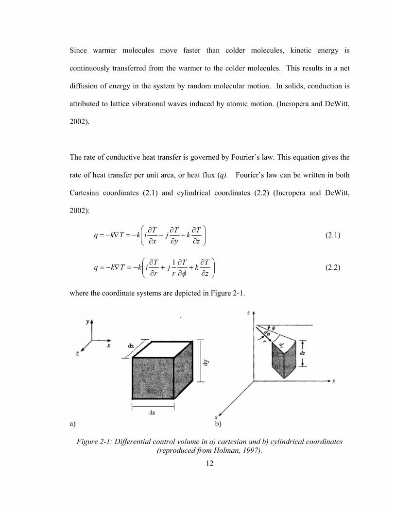
The rate of conductive heat transfer is governed by Fourier’s law. This equation gives the

rate of heat transfer per unit area, or heat flux (q). Fourier’s law can be written in both

Cartesian coordinates (2.1) and cylindrical coordinates (2.2) (Incropera and DeWitt,

2002):

⎟⎟⎠

⎞⎜⎛ ∂

+∂

+∂

−=∇−=TkTjTikTk (2.1) ⎜

⎝ ∂∂∂ zyxq

⎟⎟⎠⎝ ∂∂∂ zrr φ⎞

⎜⎜⎛ ∂

+∂

+∂

−=∇−=TkTjTikTkq 1 (2.2)

where the coordinate systems are depicted in Figure 2-1.

a)

Figure 2-1: Differential control volu ) cylindrical coordinates (reproduced from Holman, 1997).

b)

me in a) cartesian and b

12

Heat flux is a vector quantity, and as such, the conduction rate equation is written with the

del operator . It is apparent that the heat flux vector is in a direction normal to the

isotherms in an isotropic system (Incropera and DeWitt, 2002). In its cylindrical form,

the Cartesian directional components (x, y, and z) have been replaced with the radial (r),

circumferential (

∇

φ ), and axial (z) directional components. The negative sign in (2.1) and

(2.2) denotes that heat is transferred in the direction of decreasing temperature. The

variable k is known as the thermal conductivity with units of W/m·K and is a property of

the material through which the heat is transferred. In Equations 2.1 and 2.2 Incropera and

DeWitt (2002) have considered the thermal conductivity to be isotropic in nature. While

this is a valid assumption for many applications, more complex materials and mixtures

may display anisotropic thermal conductivity.

2.2.1 Thermal Conductivity

Thermal conductivity is an intensive property that describes the ease at which a material

conducts heat. It is inversely proportional to a material’s resistance to heat flow, similar

to the way electrical conductivity is an inverse measure of electrical resistivity

(Schneider, 1955). Thermal conductivity has been found to depend on the chemical

composition of the material, its phase, crystalline structure, temperature, and pressure

(Chapman, 1984; Schneider, 1955). Due to differences in intermolecular spacing, the

thermal conductivities of solids are usually greater than those of liquids, and those of

liquids are usually larger than those of gases. This range can be over more than four

orders of magnitude, as seen in Figure 2-2.

13

Figure 2-2: Thermal conductivities of a variety of materials (reproduced from Incropera

and DeWitt, 2002).

2.2.2 Specific Heat Capacity

A m (C) (J/kg·K) describes its ability to store thermal

2.2.3 Thermal Diffusivity

As defined by Inc a

measure of its ability to conduct thermal energy relative to is ability to store thermal

energy. It is measured in units of m2/s. A material possessing a high thermal diffusivity

will respond more quickly, and take a shorter time to reach equilibrium, following a

aterial’s specific heat capacity

energy. This property is determined by evaluating the amount of energy required to

increase the temperature of a unit mass of a material by one degree. Gunn et al. (2005)

defines the specific heat capacity as the material property that determines the amount of

energy absorbed or released, or the enthalpy change in a body before its temperature will

change. Specific heat capacity may be measured at constant volume (Cv) or at constant

pressure (Cp ), and is a scalar quantity.

ropera and DeWitt (2002), a material’s thermal diffusivity (α) is

14

change in its thermal environment, compared to a material with a smaller thermal

diffusivity. Thermal diffusivity is related to thermal conductivity, specific heat capacity,

and density (ρ) through:

p

kα = (2.3) Cρ

Thus, with the knowledge of any two thermal properties, coupled with the material

density, the third can be determ thermal diffusivity is often regarded as

merely a derived quantity that relates three other material properties, Hanley et al. (1978)

reinforced its significance as the physical quantity which governs the rate of heat

propagation in transient processes. It is required in order to predict a system’s response to

a transient heat source or sink. In addition to being obtained indirectly from the

measurement of thermal conductivity, density, and specific heat, thermal diffusivity can

also be determined indirectly by modeling, or directly by measurement.

2.2.4 Heat Diffusion Equation

Although Fourier’s law is useful in determining conduction heat transfer rates, it does not

of Fourier’s law. By considering a differential control volume and applying the law of

, and in

Cartesian coordinates, the heat diffusion an, 1997):

ined. Although

provide information as to how the temperature within a system varies with time (t) or

position. This data is obtained through use of the heat diffusion equation. Once the

temperature distribution is known, the heat flux at any point can be found through the use

conservation of energy, the heat diffusion equation is derived. In its general form

equation is written as (Holm

tTcq

zTk

zyk

yxk

x+⎟⎟

⎠⎜⎜⎝ ∂∂

+⎟⎠

⎜⎝ ∂∂

TTp ∂∂

=+⎟⎠⎞

⎜⎝⎛

∂∂

∂∂⎞⎛ ∂∂⎞⎛ ∂∂ ρ& (2.4)

15

16

The first three terms on left hand side of the equation represent energy inflow and outflow

through conduction, while accounts for thermal energy generation (i.e., the energy

source term), and

q&

tTc p ∂∂ρ is the energy storage term. If thermal conductivity does not

change with time, the heat diffusion equation is (Incropera and DeWitt, 2002):

tTqTTT ∂

=+∂

+∂

+∂ 1222 &

(2.5)

(Incropera and DeWitt, 2002):

kzyx ∂∂∂∂ α222

The general form of the heat diffusion equation written in cylindrical coordinates is

tTcq

zTk

zTk

rrTkr

rr p ∂∂

=+⎟⎠⎞

⎜⎝⎛

∂∂

∂∂

+⎟⎟⎞

⎜⎜⎛

∂∂

∂∂

+⎟⎠⎞

⎜⎝⎛

∂∂

∂∂ ρ

φφ&

2

11 (2.6)

2.3 Convection

⎠⎝

Convection is a heat transfer process that occurs when thermal energy is transferred

bet ee

igure 2-3) (Oosthuizen and Naylor

lectronic components in order to cool them, or, wind blowing over one’s skin.

ween a surface and a fluid flowing over it, as a result of a temperature difference (s

, 1999). Examples include a fan blowing air over F

e

Convective heat transfer involves the superposition of two individual transfer

mechanisms: the transfer of energy between the surface and fluid due to random

molecular motion (conduction), and the diffusion of heat through the fluid due to bulk

mixing by fluid motion. Heat transfer by bulk fluid motion alone is termed heat

advection.

Figure 2-3: Elements of convective heat transfer (reproduced from Oosthuizen and

Naylor, 1999).

A result of the fluid-solid interactions in convective heat transfer is the development of

boundary layers. In convection, a region near the solid surface exists where the velocity

(u) of the fluid ranges from zero to a finite value (u∞). This is termed the velocity, or

mperature varies from s f the

ulk fluid (T∞) (Incropera and DeWitt, 2002). The hydrodynamic and thermal boundary

hydrodynamic boundary layer. A thermal boundary layer will also exist where the fluid

the temperature of the solid surface (T ) to the temperature ote

b

layer profiles for the case of a fluid moving over a heated solid surface are shown in

Figure 2-4. At the interface between the fluid and the surface, the fluid velocity is zero

and heat is transferred by conduction alone. Away from the surface, warmer portions of

the fluid are bought into contact with cooler portions by the gross displacement of fluid

particles (Chapman, 1984). This forms the temperature profile seen in Figure 2-4.

17

Figure 2-4: Convective velocity and temperature boundary layer distributions, where u(y) and T(y) are the velocity and temperature distributions along the y-axis. (reproduced and

adapted from Incropera and DeWitt, 2002).

Convection heat transfer is strongly dependent on flow fields, and thus on how the flow is

gener Th fer process is termed forced convection when the

Predict n of heat

conduction, fluid dynamics, and boundary layer theory is required. These com

are frequently lumped into a single rate equation known as Newton’s law of cooling. The

equation e ween a surface and a moving fluid is (Lienhard,

1981):

ated. e convective heat trans

fluid motion is generated by an external means such as a fan, pump, or wind. When fluid

motion is a result of fluid body forces (buoyant or centrifugal) as a result of density

differences within the fluid, the resulting convective heat transfer is termed free or natural

convection (Oosthuizen and Naylor, 1999). These density changes are induced by

temperature differences within the flow region. Combined (or mixed) convection involves

fluid motion due to a combination of both body forces and external generation.

io of the convection heat transfer rate is complex as knowledge

plexities

for the convective h at flux q bet

18

)( ∞−= TThq s (2.7)

The constant h is known as the heat transfer coefficient, measured in W/m2·K, and is a

variable that takes into account the fluid composition, solid geometry, and the

hydrodynamics of the fluid motion across the solid surface (Chapman, 1984). The bar

denotes that the heat transfer coefficient is an average over the solid surface.

2.3.1 Governing Equations

In order to predict the heat transfer coefficient, the temperature, velocity and pressure

distributions in the fluid surrounding the solid surface must be determined (Oosthuizen

and Naylor, 1999). These are found by simultaneously applying the principles of

conservation of mass, momentum and energy to a control volume in the region near the

solid surface. For steady, three-dimensional flow of a viscous, incompressible fluid in a

Cartesian coordinate system with constant properties, the relevant governing equations

are (Oosthuizen and Naylor, 1999):

0=∂∂

+∂∂

+∂∂

zw

yv

xu (2.8)

⎟⎟⎠

⎜⎜⎝ ∂

+∂

+∂

+∂

−=⎟⎟⎠

⎜⎜⎝ ∂

+∂

+∂ 2

2

2

2

2

2

zyxxzw

yv

xu µρ (2.9)

⎞⎛ ∂∂∂∂⎞⎛ ∂∂∂ uuupuuu

⎟⎟⎠

⎞⎜⎜⎝

⎛∂∂

+∂∂

+∂∂

+∂∂

−=⎟⎟⎠

⎞⎜⎜⎝

⎛∂∂

+∂∂

+∂∂

2

2

2

2

2

2

zyxyzw

yv

xu µρ (2.10) vvvpvvv

⎟⎠

⎞⎜⎝

⎛∂∂

∂∂

∂∂

∂∂

⎟⎠

⎞⎜⎝

⎛∂∂

∂∂

∂∂

2

2

2

2

2

2

zw

yw

xw

zp

zw

yw

xw ⎟⎜ +++−=⎟⎜ ++ wvu µρ (2.11)

Φ⎟⎟⎠

⎞⎜⎝

⎛+⎟

⎠

⎞⎜⎝

⎛∂∂

+∂∂

+∂∂⎟

⎠

⎞⎜⎝

⎛=

∂∂

+∂∂

+∂∂

pp CxT

yT

xT

Ck

zTw

yTv

xTu

ρµ

ρ

222

⎜⎟⎜⎟⎜ 222 (2.12)

19

20

enters and leaves the

control volume entirely by advection. The variables u, v and w are the velocity

conservation of energy to the

ontrol volume results in Equation 2.12. Terms on the left hand side of the equation

Equation 2.8 is known as the continuity equation and is a result of the application of the

conservation of mass to the differential control volume. Mass

components in the x, y and z directions, respectively. Through the application of the

conservation of momentum to fluid flow, equations 2.9, 2.10, and 2.11 are derived. This

group of equations is known as the Navier-Stokes equations. The property ρ is the fluid

density and µ is the dynamic viscosity. The three terms on the left hand side of each

conservation of momentum equation represents the net rate at which momentum leaves

the control volume, while the first term on each right hand side accounts for the net

pressure force. The second terms on the right hand side of Equation 2.9, 2.10, and 2.11

represent the net viscous forces. The application of the

c

account for the net rate of thermal energy that leaves the control volume due to advection

(bulk fluid motion). This must be balanced by the net inflow of thermal energy due to

conduction, viscous dissipation and generation. The term denoted by Ф is the dissipation

function and represents the rate at which mechanical work is converted to thermal energy

due to viscous effects. Incropera and DeWitt (2002) also include an energy generation

term q& on the right side of the energy equation to account for the conversion of other

forms of energy to thermal energy. As previously stated, Equations 2.8 to 2.12 assume

constant material properties. Although this is not always the case, in many heat transfer

applications the thermal properties are not accurately known and it is common practice to

use average values if the resulting difference is less than 5-10 %.

21

is an additional change in

tent energy, it is usually associated with a change of phase (Incropera and DeWitt,

gards to phase change convection, the convection heat transfer

oefficient (h) is a function of the temperature difference Ts-Tsat, the latent heat (hfg), the

tween the liquid and the vapor, the buoyancy forces induced by density

differences between the two phases, the characteristic length of the surface, and the

2.3.2 Phase Change Convection

Typically in convective heat transfer, the internal energy transferred between the solid

surface and the moving fluid is sensible energy. When there

la

2002). The amount of energy that can be added or removed from a body before a change

of state will occur is known as the latent heat (hfg). Boiling and condensation are

characterized as forms of convection as they involve a moving fluid and a solid-fluid

interface. Because they involve a phase change, heat transfer in boiling and condensation

can occur without changing the temperature of the fluid.

Boiling is the term used to describe evaporation that takes place at a solid-liquid or liquid-

gas interface. This occurs when the temperature of the solid surpasses the saturation

temperature (Tsat) of the liquid at the measured pressure. The saturation temperature is

the temperature at which any addition of thermal energy will cause a phase change from

liquid to vapor. With re

c

surface tension be

thermo-physical properties of the liquid and vapor (ρ, Cp, µ, k) (Incropera and DeWitt,

2002). During the process of boiling, vapor bubbles grow and then detach from the solid

surface. Boiling can be characterized as either pool boiling or forced convection boiling.

In pool boiling the liquid is stagnant and all motion near the solid surface is a result of

22

temperature below the saturation

mperatu

ensation involves condensate

rmation as ind

sation.

electric resistance heater element to a ceramic stove top. Unlike heat transfer by

free convection and mixing due to bubble movement. Motion in forced convection

boiling is induced by external means such as a fan or a pump.

Condensation involves a change of phase from a vapor to a liquid at a solid-vapor

interface. This occurs when the solid surface is at a

te re of the vapor (Oosthuizen and Naylor, 1999). Latent heat is transferred from

the vapor to the solid surface and condensate forms on it. Condensation can be

differentiated by whether it is filmwise condensation or dropwise condensation. In

filmwise condensation the condensate forms as a continuous film on the solid surface and

constantly drains off as a result of gravity. Dropwise cond

fo ividual droplets that sporadically coalesce and drain off under the

influence of gravity (Oosthuizen and Naylor, 1999). The heat transfer rate during

dropwise condensation can be more than ten times greater than that associated with

filmwise conden

2.4 Radiation

2.4.1 Surface Emission

Radiation is thermal energy that is emitted from all forms of matter as a result of its finite

temperature. Energy is released by the constant oscillation and transition of electrons

within a body. This movement is maintained by internal sensible energy and hence the

temperature of the body. An example of thermal radiation would include the transfer of

thermal energy from the sun to the earth’s surface, or, the transfer of heat from a stove

23

s the propagation of

electromagnetic waves or as the propagation of photons or quanta (Incropera and DeWitt,

2002). The wavelength (λ) of these waves is given by:

conduction and convection, radiation does not require the continuous presence of matter

and is efficient within a vacuum. Thermal radiation can be viewed a

νλ c= (2.13)

where c is the speed of light in the medium (in a vacuum, c = 2.998x108m/s) and ν is the

wave frequency (Mahan, 2002). The rate at which thermal radiation is emitted per unit

surface area of a blackbody (i.e. ideal surface) is known as the emissive power of the

body (Eb) and is determined by the Stefan-Boltzmann law:

(2.14)

where σ is the Stefan-Boltzmann con l to 5.67e W/m ·K (Incropera and

eWitt, 2002). A real surface will emit less than a blackbody and follows (Incropera and

DeW

sb TE 4σ=

stant and is equa -8 2 4

D

itt, 2002):

sTE 4εσ= (2.15)

The variable ε is a property of the radiative surface and is termed its emissivity. This

value determines the efficiency of a surface, relative to a blackbody, to emit radiation.

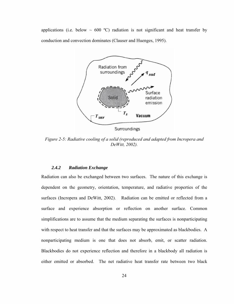
The net rate of radiation heat transfer between a solid and its surroundings is represented

in Figure 2-5. In this example both the solid and its surrounding are emitting radiation,

although, since the temperature of the solid (Ts) is greater than the temperature of the

surroundings (Tsur), the net radiative flux (qrad) is directed away from the solid (i.e. the

solid is being cooled). Due to its dependence on T4, in most low temperature heat transfer

24

inates (Clauser and Huenges, 1995).

applications (i.e. below ~ 600 ºC) radiation is not significant and heat transfer by

conduction and convection dom

Figure 2-5: Radiative cooling of a solid (reproduced and adapted from Incropera and

DeWitt, 2002).

2.4.2 Radiation Exchange

Radiation can also be exchanged between two surfaces. The nature of this exchange is

dependent on the geometry, orientation, temperature, and radiative properties of the

surfaces (Incropera and DeWitt, 2002). Radiation can be emitted or reflected from a

surface and experience absorption or reflection on another surface. Common

simplifications are to assume that the medium separating the surfaces is nonparticipating

with respect to heat transfer and that the surfaces may be approximated as blackbodies. A

nonparticipating medium is one that does not absorb, emit, or scatter radiation.

Blackbodies do not experience reflection and therefore in a blackbody all radiation is

either emitted or absorbed. The net radiative heat transfer rate between two black

25

surfaces, from a surface 1 due to interactions with surface 2 can be expressed as

(Incropera and DeWitt, 2002)

(2.16)

here A1 is the area of surface 1 , T1 and T2 are the temperatures of surfaces 1 and 2, and

F12 is a view factor or shape factor that denotes the fraction of radiation leaving surface 1

that is intercepted by surface 2. The reader is directed to Chapman (1984), or other heat

ansfe esources for an exten essions that can be used to determine F12 for

variety of geometries and configurations.

adiation exchange between non-black surfaces is more complicated than blackbody

ion must be accounted for. A frequent simplification is to

assum aque, diffuse, and gray. This means that radiation is not

o surface enclosure, the two surfaces

exchange radiation only with each other. The net radiation exchange between surfaces 1

and 2 can be determined by (Incropera and DeWitt, 2002):

:

)( 42

411211 TTFAq −= σ

w

tr r r sive list of expr

a

R

radiation exchange as reflect

e the surfaces are op

transmitted through the medium, and that the fraction of incident radiation absorbed by

the surface (absorptivity) and the emissivity are independent of radiation wavelength and

direction. In an enclosure, radiation can be reflected off all surfaces, multiple times, with

partial absorption occurring at each. In a tw

22

2

12111

1

24

14

12 111)(

AFAA

TTq

εε

εεσ

−++

−−

= (2.17)

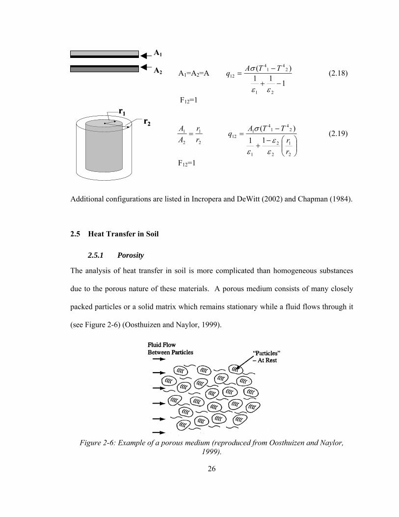
The above expression can be simplified for important special cases such as large parallel

pla d

DeWitt, 2002):

tes (Equation 2.18) and long concentric cylinders (Equation 2.19) (Incropera an

26

A1=A2=A 111

)( 24

14

−+

−σ TT (2.18)

21 εε F

12 =Aq

12=1

2

1

2

1

rA= rA

⎟⎟⎠

⎞⎜⎜⎝

⎛−+

−=

2

1

2

2

1

244

12q 11

11)(

rr

TTA

εε

ε

σ (2.19)

ed than homogeneous substances

medium consists of many closely

nary while a fluid flows through it

F12=1 Additional configurations are listed in Incropera and DeWitt (2002) and Chapman (1984).

2.5 Heat Transfer in Soil

2.5.1 Porosity

The analysis of heat transfer in soil is more complicat

due to the porous nature of these materials. A porous

packed particles or a solid matrix which remains statio

(see Figure 2-6) (Oosthuizen and Naylor, 1999).

Figure 2-6: Example of a porous medium (reproduced from Oosthuizen and Naylor,

1999).

A2

A1

r1r2

r1r2

27

Porosity (φ ) is defined by Schön (2004) as the ratio of the volume of void space (pore

space) (Vps) to the total bulk volume of the medium (V):

VV

As the porosity of rocks and soil is regional and site specific, it is difficult to provide

accurate mean values for individual groups or types.

2.5.2 Heat Transfer Mechanisms in Soil

Heat transfer in porous media is a function of he thermal properties of the solid and fluid

materials. Bear (1972) states that in a porous medium with void spaces that are filled

with a moving fluid, the three basic modes of heat transfer (i.e., conduction, convection,

and radiation) act in the following six ways:

1. Heat transfer through the sol

ps=φ (2.20)

t

id phase by conduction;

Heat dispersion is analogous to mass transfer by mechanical dispersion whereby the

presence of soil grains causes pore to pore variations in velocity, and, the thermal

conduction of heat is analogous to molecular diffusion due to concentration gradients.

This phenomenon encourages additional spreading of the heat carried by the fluid (Bear,

1972).

2. Heat transfer through the fluid phase by conduction;

3. Heat transfer through the fluid phase by convection;

4. Heat transfer through the fluid phase by dispersion

5. Heat transfer from the solid phase to the fluid phase;

6. Heat transfer between solid grains by radiation, when the fluid is a gas.

28

he conduction process

in porous media is usually described macroscopically by averaging over a representative

elementary volume (REV). Trad

2.5.3 Conduction in Porous Media

Thermal conduction in porous media is influenced by the structure of the solid matrix and

the thermal conductivity of the matrix and pore filling materials. T

itionally, conductive heat transfer analysis is carried out

under the assumption of local thermal equilibrium (LTE) between the fluid and solid

phases. Under this assumption it is presumed that at the pore scale, the local solid and

fluid temperatures are equal (i.e., Ts = Tf = T ). With this assumption, the two phase

onduction problem can be l

heat diffusion equation for the solid (s) and fluid (f) phases are averaged over an REV and

the assumption of local thermal equilibrium holds, the conduction process is described by

a single equation (Hsu, 1999):

c umped into one process. When the microscopic conduction

( ) ( )TkCC espsfpf ∇⋅∇=−+ ρφφρ 1 (2.21)

where ρf and ρs are the densities of the fluid and solid, respectively, and Cpf and Cps are the

Equation 2.21 (k ) is termed the effective thermal conductivity or the effective stagnant

es.

accurate numerical or analytical models for the effective thermal conductivity of porous

Schön, 2004). The most simplistic analytical models involve regarding each phase as

heat capacities of the fluid and solid, respectively. The thermal conductivity used in

e

thermal conductivity of the mixture and is dependent on the interfacial geometry and the

thermal properties of the solid and fluid phas

2.5.4 Effective Thermal Conductivity

The determination of experimental values for the effective thermal conductivity (ke) and

media has been the aim of many authors (see review by Hsu, 2000; Kaviany, 1991;

layers in series or parallel with respect to the direction of the thermal gradient. For solid

and fluid layers in parallel (weighted arithmetic mean), the effective thermal conductivity

can be described by (Hsu, 2000; Woodside and Messmer, 1961a):

( ) sfe kkk φφ −+= 1 (2.22)

where kf is the thermal conductivity of the fluid and ks is the thermal conductivity of the

solid. For solid and fluid layers in series (weighted harmonic mean) the effective thermal

conductivity is represented by (Hsu, 2000):

( )φφ −+⎟⎟⎠

⎞⎜⎜⎝

⎛=

1f

s

se

kk

kk (2.23)

yers in series. These represen imum effective thermal

l conductivity, as long as the solid and fluid thermal conductivities are

ot significantly different.

2.5.5 Convection in Porous Media

porous media, fluid flows through the pore spaces between the solid particle grains. If a

The effective thermal conductivity for layers in parallel is always larger than that for

t the maximum and minla

conductivity values. The weighted geometric mean model provides a practical,

intermediate approximation of ke and is represented by (Woodside and Messmer, 1961a):

φφ −= 1sfe kkk (2.24)

According to Nield (1991), the geometric mean model provides a good estimate of the

effective therma

n

Heat transfer by convection requires the movement of fluid over a solid surface. In

plane is drawn in a porous media, the velocity will not be uniform over the plane (Figure

29

30

2-7). A common simplification to this flow

velocity. By integrating the local velocity over a representative area that is small

tem

problem is the use of an area averaged

compared to the sys but larger than pore scale, the mean velocity v in the x, y and z

directions can be found.

Figu Ve n across a vertical plane in a porous medium (reproduced re 2-7: locity distributio

from Oosthuizen and Naylor, 1998).

As with convection in nonporous materials, analysis of heat transfer by convection in

porous media requires the simultaneous application of the principles of conservation of

mass, momentum to a control volume. With the use of the volume-averaged velocity, the

continuity equation for flow in a porous media is equivalent to that used for a pure fluid

(Equation 2.8).

Applying the law of conservation of energy to a porous control volume results in energy

equations for the fluid and the solid phases. Under the assumption of LTE, these energy

equations can be combined into a phase averaged equation. Ignoring viscous dissipation

and energy generation, the energy equation is represented by: (Lauriat and Ghafir, 2000):

( ) ( ) ( ) ( )TkTvCpTC ∇∇=∇⋅+∂ ρρ (2.25)

where the term

t afep ∂

( )epCρ is a combination of the fluid and solid densities and heat capacities

and can be estimated by:

( ) pffpssep CCC φρρφρ +−= )1( (2.26)

The term ka is the apparent thermal conductivity and is function of the effective stagnant

thermal conductivity (ke) of the solid and fluid, as previously discussed, and the

dispersion conductivity (kd). The thermal dispersion conductivity accounts for additional

heat transport due to transverse and longitudinal dispersion within the pores as a result of

tortuous flow paths (Lauriat and Ghafir, 2000).

2.5.6 Boiling in Soil

T

eat source, at a temperature higher than 100 ºC is applied to a one-dimensional, water

are created: a zone clos

inates, a

two-phase convective zone characterized by evaporation and condensation, and a cool,

onduction dominated, l

Conduction heat transfer in the vapor filled zone creates steep temperature gradients. In

the convective zone, water saturation varies, while the temperature is relatively constant

ler temperatures in the

liquid saturated zone cause steam condensation, increasing water saturation and

he study of phase change in soil is often simplified to a one-dimensional problem. If a

h

saturated porous medium, three distinct regions est to the heater

which contains pore water that has been vaporized and where conduction dom

c iquid filled zone (Udell, 1985; Satik, 1997)) (Figure 2-8).

and equal to the boiling point of water at the local pressure (Baker and Heron, 2004;

Ramesh and Torrance, 1990). Evaporation of pore water in this zone causes a decrease in

water saturation and an increase in the local capillary pressure. Coo

31

32

vapor concentration

countercurrent flow of water vapor towards the liquid filled zone and liquid water

decreasing s. These pressure and vapor gradients cause a

towards the heated vapor zone by a capillary pressure gradient (Baker and Heron, 2004).

Figure 2-8: Vapor, two-phase, and liquid zones with corresponding temperature profile during boiling in porous media (adapted from Udell, 1985).

The countercurrent mass fluxes of liquid (m m) and vapor (& l & v), related to the pressure

gradient, can be found through (Udell, 1985):

dx

l

l

rl (2.27) dKKm ll

Φ=

µρ

&

2

dxdKK vrvv Φρ 2

mv

v = µ& (2.28)

where, K is the permeability of the porous media, Krl and Krv are the relative

permeabilities of the porous media to the liquid and vapor phases respectively, x is the

distance, and Φl,v is the fluid potential as defined by (Udell, 1985):

Θ+≡Φ sin,

, gxP

vl

vl

ρ (2.29)

where P

,vl

l,v is the pressure of the liquid or the vapor, g is gravitational acceleration, and Θ

denotes the angle between q and x (see Figure 2-9), therefore, for horizontal heating, Θ is

equal to zero and the second term in Equation 2.29 is disregarded.

Figure 2-9: Direction of heat flux relative to the vertical (x) direction.

The difference between the liquid and vapor pressures P and P is defined as the capillary

pressure (P ):

l v

c

Pc = Pv - Pl (2.30)

e temperature gradients in the two-phase region are slight, the energy equation

(2.31)

where Q is the heat transfer rate and hfg is the latent heat.

2.6 Thermal Properties of Soil and Rock

he thermal properties of soils have been experimentally determined and published in

any journals and handbooks, however, a broad range of values is often observed. This

Since th

can be reduced to:

fgvhmQ &=

T

m

33

34

is -1

summariz city, and

ther sivity for t soil Th are

dependent on porosity and water saturation, mi osition, grain erature,

and pressure, with water content displaying the greatest variation under field conditions

(Lu et al., 2007). Many authors have attempte l

properti of soils from ge of the min ituent, saturation, porosity, and

tem lauser a s, 1995; Seipold, 1998; Gunn et al., 2005; Vosteen and

Schellschmidt, 2003; Woodside and Messmer, 1961a), but each model has its own faults.

Som eters which are difficult to obtain, and others, do

not perform well at lower water contents or ils (Lu et al., 2007).

Some overestimate while others underestimate, and, most are only valid for a specific

range of values.

because the thermal properties of soils are extremely site specific. Table 2

es a number of published values of thermal conductivity, heat capa

mal diffu differen and rock materials. ermal properties

neral comp size, temp

d to derive models to predict the therma

es knowled eral const

pera re (Ctu nd Huenge

e require a long list of input param

with fine textured so

35

Schön, 2004 except: Cermak and Rybach, 1982, Adapted from Jumikis, 1977, Bejan

Conductivity (W/m·K) Pressure (kJ/kg·K) (m /s x 10 )

Table 2-1: Thermal Properties of Some Common Soil and Rock Types. Values from 1 2 3

and Kraus, 2003, 4 U.S. Dept. of Defense, 2006, 5 Chirdon et al., 2007

Material Thermal Heat Capacity at Constant Thermal Diffusivity 2 -7

Clay 0.60…2.60 0.84…1.00 2.5…10.21

0.38…3.02 0.75…3.55 2.54…11.6 (dry) 0.14…0.24 9.722

(sandy) 0.94 Granite 1.25…4.45 0.67…1.55 5.0…17.61

2.3…3.6 7.52

1.34…3.69 0.74…1.55 3.33…15.0 1.12…3.85 0.25…1.55 3.33…16.5

Gravel mean 1.841 Limestone 0.62…4.40 0.82…1.72 5.0…12.21

1.30…6.26 6.112

0.92…4.40 0.75…1.71 3.91…16.9 Peat 0.60…0.80

(dry) mean 0.11 (moist) mean 0.46

Quartzite 3.10…7.60 0.71…1.34 14.8…20.91

2.33…7.45 13.6…20.9 2.68…7.60 0.72…1.33

Sand 0.10…2.75 1.97…3.18 3.5…6.01

1.70…2.50 (dry) 2.192

0.18…3.49 (dry silty sand) 9.764

1.63…4.75 (wet silty sand) 5.824

(dry) 0.584 1.75

(moist) 1.13 San 6.112dstone 0.90…6.50 0.75…3.35

1.88 .98 2.…4 54…20.4 0.38…5.17 …3.35 0.67 2.50…4.20 (dry) 0.67…6.49 (m oist)1.10…7.41 (oil sat) 0.84…4.24

Soil 0.60…3.33 (dry) 0.8372 44

(dry) 1 1.84 (wet) 2

2.6.1 Dependence on Porosity and Saturation

The thermal properties of soils and porous sedimentary rocks are dominantly influenced

by porosity and saturation (Schön, 2004). A soil’s thermal behavior is dependent on the

differences in thermal properties between the solid mineral matrix and the pore filling

36

material (Sorour et al., 1990). Since the thermal conductivity of solids is generally

greater than liquids or gases, as the porosity of the soils increases, the amount of pore

filler also increases, and, the overall thermal conductivity of the soil decreases. Figure 2-

10 shows the difference in thermal conductivity values between air, oil, water, and

minerals. At equivalent porosity, a soil saturated with water will have a higher thermal

conductivity than a soil saturated with oil, or with air (Woodside and Messmer, 1961b).

Experimental results from Sorour et al. (1990) showed a nearly linear increase in thermal

conductivity with increasing moisture content, as the number of pore spaces containing

ai l

onductivity of sand and consolidated sandstone to pore filling material is illustrated in

Figure 2-11.

r decreased and those containing water increased. The sensitivity of therma

c

1e-2 2e-2 5e-2 1e -1 2e-1 5e-1 1 2 5

(W/m·K)

Figure 2-10: Thermal conductivities of common pore filling materials and minerals (reproduced and adapted from Schön, 2004).

Figure 2-11: Thermal conductivity vs. porosity for sandstone and sand saturated with

water, oil and air (reproduced from Schön, 2004 - after Woodside and Messmer, 1961b).

Sorour et al. (1990) found thermal diffusivity to increase with increasing moisture content

when measured at 10, 20, 30, and 40% saturation. Hanley et al., (1978) measured the

thermal diffusivity of eight well-characterized rocks and found that all eight rocks types

sampled had higher thermal diffusivities in the water saturated state than in the air dried

tate. Even though the thermal diffusivity of water at 20 ºC is 1.51e-7 m2/s while the

and the other thermal

properties is that the heat capacity of water (4.187 kJ/kg·K) is very high is comparison

s

thermal diffusivity of dry air at 20 ºC is significantly higher at 2.12e-5 m2/s (Schön,

2004), the thermal diffusivity of soil increases with increasing moisture content due to its

relationship with thermal conductivity (Equation 2.3) and the significant increase in

thermal conductivity with increasing moisture content.

Like thermal conductivity, the specific heat of air is lower than that of oil, which is lower

than that of water. The main distinction between specific heat

37

38

2.6.2 Dependence on Mineral Composition

rocks to a lesser extent, is also a function of the thermal

cond o nstituents (Sundberg, 1988; Schön, 2004).

rocks and

sands, and their quartz content. This thermal property has been shown to increase with

with most minerals. This means that the contribution of pore water to the overall specific

heat of a soil is significant (Gunn et al, 2005). In general, heat capacity increases with

increasing moisture content (Sorour et al., 1990; Bejan and Kraus, 2003).

Although the thermal conductivity of most soils and sedimentary rocks is mainly

controlled by porosity and saturation, the thermal conductivity of denser rock types, and

soils and sedimentary

uctivity f its dominant mineral co

Mineral classes can be arranged by decreasing thermal conductivity: native metals and

elements such as graphite and diamond (mean 120 W/m·K), sulfides (mean 19 W/m·K),

oxides (mean 11.8 W/m·K), fluorides and chlorides (mean 6 W/m·K), carbonates (mean 4

W/m·K), silicates and sulfates (mean 3.3 and 3.8 W/m·K), nitrates (mean 2.1 W/m·K),

and native elements/nonmetals such as selenium and sulphur (mean 0.85 W/m·K)

(Kobranova, 1989).

Correlations have been made between the thermal conductivity of metamorphic

increasing quartz content (Clauser and Huenges, 1995; Schön, 2004). As seen in Table 2-

1, quartzite, which is high in quartz content, has been shown to have a thermal

conductivity ranging up to 7.6 W/m·K. This is higher than any other metamorphic rock.

In plutonic (igneous) rocks, high feldspar content has been shown to bias thermal

conductivity towards lower values (Clauser and Huenges, 1995).

39

and rocks with high feldspar content have intermediate values

anley et a., 1978).

2.6.3 Dependence on Grain Size

found higher values of thermal conductivity for

andy soil than for clay loam soil. Since particles are not uniformly shaped and do not fit

Tavman, 1996).

re

The thermal diffusivity of rocks is also dependent on its mineral composition (Hanley et

al., 1978). Similar to thermal conductivity, the thermal diffusivity of igneous and

metamorphic rocks was found by Hanley et al (1978) to be strongly dependent on quartz

content and to a lesser extent on feldspar and calcite content. Rocks with high quartz

contents show the highest thermal diffusivities, while those of high calcite content have

low thermal diffusivities,

(H

For dry samples, a correlation was made by Sorour et al. (1990) between thermal

conductivity and grain size. It was found that the thermal conductivity of dry pure sand

was higher than dry pure clay, with sandy-clay and clayey-sand mixtures lying between.

Abu-Hamdeh and Reeder (2000) also

s

together perfectly, as grain size decreases, the number of inter-grain spaces increases and

the thermal resistance between particles increases. This results in a decrease in thermal

conductivity (Schön, 2004; Abu-Hamdeh and Reeder, 2000;

2.6.4 Dependence on Temperatu

The thermal conductivity and thermal diffusivity of many rocks have been found to

decrease with increasing temperature (Hanley et al., 1977; Vosteen and Schellschmidt,

2003; Robertson, 1988). Rocks with large thermal conductivity at ambient temperature

show a more pronounced decrease with increasing temperature than those with a low

thermal conductivity at ambient temperature. Vosteen and Schellchemidt (2003) showed

that thermal diffusivity decreases more than thermal conductivity with increasing

40

al

onductivity of dry sand and dry clay with temperature increasing from 0 ºC to 35 ºC. It

so dependent on temperature. It has generally

been found to increase with increasing temperature (Robertson, 1988). However, as

reported by Hanley et al. (1977), the dependence is slight.

2.6.5 Dependence on Pressure

Increasing pressure causes the thermal conductivity of rocks and soils to increase,

although, the effect of temperature is far more significant (Bear, 1972; Abdulagatov et al.,

2006). At low pressures, thermal conductivity steadily increases due to an decrease in

porosity and the closure of microcracks, fractures, and pores, and to the improvement of

therm

increase, eventually all of these cracks and pores become closed and the effect of pressure

temperature. Hanley et al. (1978) found that above 800K, the thermal diffusivity of some

rocks gradually increases with temperature. This was attributed to the increasing

importance of radiation heat transfer. Hanley et al. (1978) also found that rocks that have

a high diffusivity will show a stronger temperature dependency than ones that are poor

conductors (low thermal diffusivity). This temperature dependency decreases with

increasing temperature.

Although fewer studies have examined the relationship between thermal conductivity of

soil and temperature, a study by Sorour et al. (1990) found a slight increase in therm

c

was also found that the thermal conductivity increased with decreasing negative

temperature (i.e. from 0 ºC to -10 ºC).

The specific heat capacity of rocks is al

al contact at grain and crack boundaries (Schön, 2004). As pressure continues to

41

ases, leading to a linear leveling off of thermal conductivity

alues (see Figure 2-12) (Cermak and Rybach, 1982; Clauser and Huenges, 1995). In

pressure dependency on thermal conductivity may not occur and the dependence on

pressure may only be slight. An interesting result is the effect of vacuum or negative

pressure on the thermal conductivity of rocks. Measurements made on basalt samples

showed that applying a vacuum caused a decrease in thermal conductivity (Robertson,

1988). Although other rocks were not studied, Robertson (1988) inferred that the

observed decrease in k would occur in other rock types as well.

The relationship between thermal diffusivity, specific heat capacity, and increasing or

decreasing pressure has not been well studied. Theories have shown however, that there

is little pressure dependence on the specific heat of solids and liquids until very high

pressures are reached (Chapman, 1984).

on thermal conductivity decre

v

dense, and essentially non-compressible rocks with few fractures, the initial rise in

Figure 2-12: Thermal conductivity vs. pressure for a gneiss rock sample (reproduced

from Schön, 2004.

42

2.7

In-Situ thermal treatment technologies involve the application of heat to the subsurface as

a means to mobilize and remove contaminants. These technologies have become

increasingly popular due to their ability to overcome the rate-limiting properties of

traditional remediation techniques. Several mechanisms have been identified as

contributing to the enhanced contaminant recovery reported with in-situ thermal

remediation techniques. These include: evaporation/vaporization, boiling, increase in

Henry’s Constant, increase in solubility, decrease in viscosity, decrease in adsorption, and

the creation of permeability.

A number of technologies have been designed as methods of increasing the temperature

E), trichloroethylene (TCE),

nd poly-chlorinated biphenyls (PCBs), as well as light non-aqueous phase liquids

(LNAPLs) have been treated using these technologies.

Thermal Remediation

of the subsurface. These include: electrical resistive heating (ERH), thermal conductive

heating (TCH), and steam enhanced extraction (SEE). ERH involves conducting an

electrical current through the subsurface to produce thermal energy. In TCH, the

subsurface is heated through thermal conduction from heater wells. Steam is injected into

the subsurface through wells in SEE.

In situ thermal heating methods were first developed by the petroleum industry for

enhanced oil recovery and were later adapted for soil and groundwater remediation

(USEPA, 2004). DNAPLs such as tetrachloroethylene (PC

a

43

2.7.1 Mechanisms for Contaminant Removal

2.7.1.1 Vaporization and Boiling

Evaporation is the process by which a substance in the liquid state is transformed into the

gas phase at a temperature below the boiling point of the substance. The total pressure of

the gas phase is described by Dalton’s law. Dalton observed that the total pressure of a

gas mixture (Pt) is equal to the sum of the partial pressures (vapor pressures) of each

component (Mahan and Myers, 1987):

(2.32)

The mole fraction of component 1 in the gas phase (Y1) is related to the partial pressure

by (Oxtoby et al., 1999):

he vapor pressure rium with its non-

be the tendency of a liquid to vaporize or

mperature and

f some common groundwater contaminants

is plotted against T and 1000/T. It can be seen that

nt PPPPP ...321 +++=

tPYP 11 = (2.33)

is the pressure exerted by a vapor that is in equilibT

vapor phases. It is often used to descri

evaporate. A substance with a high vapor pressure at moderate temperatures is usually

referred to as volatile. The boiling point of a mixture is the temperature at which the

vapor pressure is equal to atmospheric pressure. Vapor pressure rises rapidly with

te thus, increasing temperature causes an increase in the volatility of a

solution. In Figure 2-13, the vapor pressure o

as T decreases from 400 ºC to 0 ºC,

the vapor pressure of all contaminants listed also decreases.

Figure 2-13: Vapor pressure vs. temperature for common groundwater contaminants

In an ideal, miscible solution, the vapor pressure (partial pressure) of component 1 (P1) is

(reproduced from Stegemeier and Vinegar, 2001).

related to the mole fraction of component 1 in the liquid phase (X1) and the pure

component vapor pressure (P1°) through Raoult’s Law (Mahan and Myers, 1987):

°= 111 PXP (2.34)

Therefore, the total pressure of the system is:

44

°+° nn PXP ...4 (2.35) +°+°+°=t XPXPXPXP 4332211

ith the composition of the solution and will always be

liquid composition (given by the lower curve) the boiling point will be between the

As the boiling point is dependent on the vapor pressure of the system, the boiling point of

an ideal, miscible mixture varies w

between the boiling points of the individual components. In Figure 2-14, at any given

45

t temperature.

individual component boiling points (T1b and T2

b), and the resulting vapor composition is

given by the position of the upper curve at tha

Figure 2-14: Boiling point of an ideal, miscible solution as a function of the composition of the liquid (mole fraction of the components in the solution) (reproduced from Oxtoby et

al., 1999).

Immiscible mixtures present a deviation from Raoult’s law as the presence of one

component does not affect the properties of the others. The total vapor pressure of the

system is independent of the mole fractions of each component and is related only to the

pure vapor pressure of each individual component (Smith and Van Ness, 1987):

°+°+°+°+°= nt PPPPPP ...4321 (2.36)

For both miscible and immiscible mixtures, each pure component vapor pressure (P °)

can be found by the ideal gas law:

n

VRT

nn nP =° (2.37)

46

where nn is the number of moles in the gas phase, R is the universal gas constant, T is the

temperature, and V is the volume of the gas.

In a solution of immiscible liquids that is well stirred, boiling begins when the total vapor

pressure of the mixture reaches atmospheric pressure. Mixtures of chlorinated solvents

and water in the subsurface will boil at a temperature lower than the boiling point of

water or of the individual contaminants (USEPA, 2004). This process is termed steam or

co-distillation. It is especially useful in vaporizing contaminants with very high boiling

points such as PCB’s and polynuclear aromatic hydrocarbons (PAHs). In Figure 2-15,

the vapor pressure of PCE, water, and an immiscible mixture of PCE and water is plotted

as e

m

perature than either of the individual components. For a PCE and water mixture this

tem

ell m ate into es

a smal (0.02 wt d in it wt %

PCE with <0.01 wt % of water dissolved in it (Hodgman et al., 1962). When heated, the

sys 8.5 °C and the dissolved substances are purged from their solution

(A , 2006). This boiling results in vigorous agitation of the mixture

hich allows each liquid phase to be continuously replenished with the dissolved

component (Atkins and de Paula, 2006). Boiling continues until one immiscible phase has

been depleted. In Table 2-2 the boiling point and co-distillation points of some common

chlorinated solvent and water mixtures are listed.

a function of increasing temperature. It can be seen that the vapor pressure curve of th

iscible mixture will be equal to atmospherics pressure (1.01 bar) at a lower im

tem

perature is 88.5 ºC (Horvath, 1982). At equilibrium, PCE and water that have been

w ixed will separ

l amount

two distinct phas

%) of PCE dissolve

: one composed of 99.8 wt % water with

and another composed of 99.99

tem co-boils at 8

tkins and de Paula

w

Figure 2-15: Vapor pressure of PCE, water, and PCE-water immiscible mixture as a function of increasing temperature (reproduced and adapted from Costanza, 2005).

Table 2-2 – Boiling points and co-distillation temperature of some common DNAPLs

Solvent Boiling Point (°C) -Distillation Point of Chlorinated Solvent - Water Mixture (°C)

(adapted form USEPA, 2004).

Chlorinated Pure Substance Co

Tetrachloroethylene 121 88 Trichloroethylene 87 73

1,1,2- 114 86 Trichloroethane Tetrachloromethane 77 67 Trichloromethane 61 56 Dichloromethane 40 39

Co-distillation requires the presence of an immiscible mixture, thus dissolved phase

chlorinated solvents do not exhibit the behavior seen in Figure 2-15. The total vapor

pressure and thus boiling point of dissolved phase chlorinated solvent systems will follow 47

48

action of water (X2), the

effect of the dissolved phase on the total vapor pressure is nearly negligible.

) describes the partitioning of a substance in the gas and liquid

phases. It is the ratio of the gas phase concentration (Cg) to the dissolved concentration

Raoult’s law (Equation 2.35), but as a result of their low solubility, the mole fraction of

the contaminant (X1) is very low in comparison to the mole fr

Once the pure boiling point of a contaminant has been reached, it will vaporize

independent of whether water, air, or another solvent/solute is present in the subsurface.

Boiling points of contaminants range from 80°C for benzene to 524°C for

dibenzo(a,h)anthracene (Stegemeier and Vinegar, 2001). During ERH and steam

injection, the maximum achievable temperature is the boiling point of water, therefore,

only volatile, low boiling point contaminants will reach their boiling point. Refer to

Chapter 1, Table 1-1 for the boiling points of some common DNAPLs.

2.7.1.2 Increase in Henry’s Constant

The Henry’s Constant (H

(Cw) of a substance at equilibrium (Heron, 1998b):

w

gCH = (2.36)

C

Therefore, as the Henry’s constant of a contaminant increases, the concentration in the

gas phase also increases and the dissolved concentration decreases. Heron et al, (1998a)

measured the Henry’s constant of TCE between 10 and 95 ºC and found it to increase by

a factor of 20. It was concluded that large effects on volatility could be expected during a

thermal remedy. A 2002 study by Shimotori and Arnold measured the Henry’s constant

of PCE, TCE, and DCE (dichloroethylene) in a number of solvents including alcohols and

49

2.7.1.3 Increase in Solubility

As the subsurface temperature is increased, the viscosity of liquid contaminants

decre o ch as TCE, PCE, DCE, and other chlorinated

The tendency of a contaminant to adsorb onto the surface of solid soil grains is a function

of the solid specific area, fraction organic carbon, partitioning of the contaminant in the

water from 0.2 to 70 ºC. The Henry’s law constant was found to increase with

temperature for each contaminant and in all solvents analyzed.

Knauss et al. (2000) studied the aqueous solubility (S) of TCE and PCE as a function of

temperature between 20.85 and 116.85 ºC for TCE and between 21.85 and 160.85 ºC for

PCE. The solubility of TCE was found to increase from 0.010763 mol/L to 0.037889

mol/L in this temperature range, while the solubility of PCE increased from 0.001157

mol/L to 0.013729 mol/L. Other authors have measured the dependence of temperature of

the solubility of chlorinated hydrocarbons at lower temperatures and have found similar

trends (Heron et al., 1998a; Horvath, 1982). These results are significant as increasing

solubility will increase the mass transfer of contaminants from the NAPL phase into the

aqueous phase where they are more easily mobilized by traditional treatments methods

such as pump-and-treat.

2.7.1.4 Decrease in Liquid Viscosity

ases. F r organic contaminants su

solvents, this change is viscosity is about one percent per degree Celsius (Davis, 1997).

Decreasing viscosity allows for the heated liquids to move more freely through the

subsurface, aiding in the recovery of contaminant from recovery wells.

2.7.1.5 Decrease in Adsorption

50

cient Kd, describes the distribution of

contaminant between the aqueous and sorbed phases. A decrease in (Kd) corresponds to

the subsurface is heated above the boiling point of water, as is the

case in many TCH treatments, as the soil dries, it shrinks, develops fractures and becomes

desiccated (Stegemeier and vinegar, 2001). This increases the permeability of the soil

and aids in the mobilization of contaminant and water vapors, and, increases the

effectiveness of the vapor extraction system. At high temperatures, the removal of

liquid and gas phases, and a strong function of temperature (Udell, 1997). It has been

found that an increase in temperature will shift the contaminant equilibrium from the

more dense to the less dense phases (i.e., from soil to liquid, liquid to gas or solid to gas)

(Isherwood et al., 1992). The distribution coeffi

an increase in concentration of contaminant in the aqueous phase and a decrease in the

concentration sorbed to the solid soil grains. In a study by Sleep and McClure (2001),

column experiments were performed to determine the distribution coefficients for

toluene, PCE, and naphthalene at 20 ºC, 50 ºC and 92 ºC in order to determine the impact

of temperature on the sorption of these compounds. It was found that increasing soil

temperature from 22 - 25 ºC to 90 ºC significantly decreased the distribution coefficient

for all contaminants analyzed. In another study by Uzgiris et al. (1995) similar results

were achieved when studying the desorption of PCBs from soils and sediments. Results

showed that the residual PCB concentration in soil heated in a convection oven decreased

faster and to a lower final concentration level with increased temperature.

2.7.1.6 Creation of Permeability

As soil heats during a thermal treatment, the liquid saturation decreases as pore water is

removed. This decrease in liquid phase increases the relative permeability of the gas

phase in the soil. If

51

organic matter can also contribute to increased porosity and permeability (Vinegar et al,

1997). In a field demonstration, Vinegar et al. (1997) found that soil samples that had

been thermally treated for 42 days had a significantly higher air permeability and porosity

than pre-treatment samples (Vinegar et al., 1997).

2.7.2 Electrical Resistive Heating

Electrical resistive heating is a remediation technology whereby electrical energy

generated in the subsurface as a result of resistance to electrical current between

electrodes, is transformed to thermal energy (Truex et al., 2007). Thermal energy

pro ce

onduction of between the electrodes. This

t into the subsurface, but are also used for vapor removal. Recovered vapors are

treated ex-situ using conventional methods (Truex et al., 2007). Figure 2-16 depicts a

typic

pagates through the treatment zone via thermal conduction. It is the subsurfa

moisture which allows for electrical c

technology was originally developed as a dewatering tool at the Pacific Northwest

National Laboratory in the early 1990s but became a stand alone remediation technology

in 1997 (Beyke and Fleming, 2005). Once a contaminated site has been chosen for

remediation via ERH, a series of electrodes are placed throughout the treatment area, with

a typical electrode spacing of between 4 m and 8 m. Closer spacing results in higher

installation costs, but a shorter operating time. These electrodes conduct alternating

curren

al ERH setup.

Figure 2-16: Schematic representation of ERH system setup (adapted from USEPA, 2004).

Resistance in the subsurface is mainly determined by the moisture content, concentration

of dissolved salt or ionic content of the water, and ion exchange capacity of the soil itself

(USEPA, 2004) Moisture in the vadose and saturated zones will conduct electricity thus

treatment can be carried out in both saturated and unsaturated zones, as long as moisture

is present. Once pore water has been eliminated, resistive heating can no longer function,

and thus, the maximum operating temperature for ERH is the boiling point of water (100

°C)

2.7.3 Thermal Conductive Heating

Therm du er soil remediation technology that involves

s

e

.

al con ctive heating (TCH) is anoth

the simultaneous application of thermal energy and vacuum to a contaminated site. Well

containing electrical heating elements are installed in a hexagonal grid pattern, with a

well containing a heater element and vacuum (heater/vacuum well) positioned in th

52

53

n

,

o

o

r

s

centre of each hexagon (see Figure 2-17) (Baker and Heron, 2004). Heat is transferred

through the subsurface by conduction from the heater wells, promoting the mobilizatio

and/or destruction of contaminants via evaporation, steam distillation, boiling, oxidation

and thermolysis. Simultaneously, a vacuum is applied to each heater/vacuum well t

capture the vapors that are generated. Soil temperatures typically reach from 100 t

500ºC, depending on the compound in question; lower temperatures are commonly

employed for volatile, low boiling point contaminants (e.g. TCE, PCE, BTEX) and highe

temperatures are required for semi-volatile compounds (e.g. PCBs, and manufactured ga

plant wastes) (Stegemeier and Vinegar, 2001).

Figure 2-17: Heater/Heater-Vacuum Well Configuration (Stegemeier and Vinegar, 2001).

2.7.4 Steam Enhanced Extraction

SEE involves the injection of steam into the subsurface and the subsequent extraction

of produced vapors and liquids for ex situ treatment (see Figure 2-18). A SEE system

usually consists of a series of steam injection wells and extraction wells arranged in a

pattern similar to the one used for TCH with a ring of injection wells surrounding a

54

d viscosity (Davis, 1998). The approaching steam front induces vaporization,

evaporation and steam distillation of the compounds.

central extraction well (USEPA, 2004). As steam moves through the subsurface

towards the region of contamination, three zones are formed: a steam vapor zone, a

two-phase variable temperature zone, and a liquid zone. Refer to section 2.5.6 for a

discussion of the properties of each region. The first zone to come into contact with

the contaminant is the liquid water zone. This cold water flushes the contaminants

from the pores, while the following two-phase zone increases the subsurface

temperature enhancing the ease and rate of mobilization to recovery wells through

decrease

Figure 2- 18: Schematic representation of a steam enhanced extraction (SEE) process (Davis, 1998).

Steam injection has a major disadvantage in that it can only be injected into relatively

permeable zones (Heron et al., 1998b). As steam cannot readily penetrate low

permeability soil, high heat losses and the possible inability to completely heat the area

55

sult. Hydraulic conductivity can vary by 10 orders of magnitude at a single site,

2.7.5 Laboratory Studies

ber of pilot and field studies have examined the feasibility of in situ

ermal remedy techniques for DNAPL remediation (e.g., Heron et al., 2005; LaChance

a decrease in average soil TCE concentration from 271 to 0.6 mg/kg.

re

resulting in some areas of the target zone being bypassed. In contrast, thermal

conductivity varies by a factor less than 10 through all soil types. Therefore, technologies

such as ERH and TCH are applicable in tight soils and clays, independent of

heterogeneity, permeability, moisture content or stratigraphy (Stegemeier and Vinegar;

2001; Heron et al., 1998b). SEE has been combined with ERH at a number of field sites

in order to improve mobilization of contaminants in low permeability zones (USEPA,

2004).

Although a large num

th

et al., 2004; Hudson et al., 2002, 2006; Tse et al., 2001), very few laboratory experiments

have been conducted to confirm the results of these studies or to understand the

underlying processes involved.

Heron et al. (1998b) simulated ERH in a 2-D laboratory tank for TCE removal from a

silty soil. For an initial 8 days, soil vapor extraction alone was used and only 6.8% of the

initial TCE was removed from the tank. After this initial period, the temperature of the

soil was increased to 85 ºC. After 28 days of heating at 80 - 90 ºC, 55 % of the total TCE

had been removed from the box although a steady state flux of only 0.35 g/day was

reached. The soil temperature was then increased to 99 - 100 ºC and after only 5 days of

pore water boiling, 13.9 grams of TCE had been removed, resulting in 99.8 % mass

removal and

56

1998, Hansen et al. conducted a series of treatability studies in order to determine the

(MGP) wastes to residual levels. 50-100 g soil samples impacted with coal tar were

heated in a muffle oven at temperatures from 200-400 ºC, depending of the boiling point

of the contaminant of interest. It was found that volatile compounds such as benzene

could be reduced from 39,000 µg/kg to 22 µg /kg after 1 day of heating at 200 ºC. Semi-

volatile contaminants were treated at higher temperatures and for longer periods of time.

Better results were seen after heating at 300 ºC for three days as opposed to 400 ºC for

one day.

The removal of PCE from soil using steam injection was examined by She and Sleep

(1999). A bench scale parallel plate chamber was constructed with two vertical injection

wells and filled with sand. Free phase PCE-DNAPL was completely removed with a total

PCE recovery of 84 %. Downward migration of PCE was observed past a finer grained

silica sand layer. A laboratory study was conducted by Sleep and McClure, (2001) to

evaluate the efficiency of SEE for removal of VOCs and semivolatile organic compounds

(SVOCs) from a gravelly till soil, and to compare the contaminant removal rate achieved

with SEE with that of air flushing. The application of SEE following air flushing

increased both VOC and SVOC removal rates. After 11 pore volumes of steam

condensate had been passed, the total VOC soil gas concentration had been reduced by a

factor of 20 and the total SVOC concentration in the steam condensate decreased from 11

In

temperature and time at elevated temperature required to reduce Manufactured Gas Plant

to 3 mg/L.

57

In the past 20 years, traditional sampling techniques for VOC analysis have involved

using a spatula type device to completely fill a large jar or bottle with bulk soil in the

field. This soil was then transferred off site to a laboratory where an aliquot of the

material was placed in water before analysis (Liikala et al., 1996). These containers were

often cooled to 4 ºC and kept for up to 14 days before analysis. During the 1990’s many

d validity of this bulk sampling method.

Several authors revealed large negative biases associated with this method and losses in

excess of 90 % before analytical measurement in some cases, due to the high vapor

pressures and volatilities at ambient conditions characteristic of these compounds

(Siegrist and Jenssen, 1990, Liikala et al., 1996). The extent to which VOCs are lost to

concentration, surface area exposed, duration of exposure, porosity of matrix, temperature

and pressure (ASTM, 2006; Siegrist and Jenssen, 1990). In 1997, The Environmental

Protection Agency’s “Test Methods for Evaluating Solid Waste”, SW-846 Method 5030

was updated to reflect these findings. The practice of packing soil into a jar for later

preservation were published in a Method 5035 (USEPA, 1996).

EPA Test Method 5035 was updated again in July 2002 to 5035A (USEPA, 2002). It

discusses recommended procedures for sampling, handling, and preserving soil samples

and biodegradation by emphasizing that samples be collected only from freshly exposed

2.8 Post-Remedy Sampling Techniques for VOC analysis

studies were conducted to assess the accuracy an

the atmosphere is a function of the soil sorption affinity of the target VOC, vapor phase

analysis was removed and new procedures for sample collection, handling, and

for VOC analysis. These procedures are designed to limit VOC losses by volatilization

58

exposed, it is recommended that sub-sampling be done with the

se of a metal or rigid plastic coring tool or syringe in order to help maintain the sample

sport (USEPA, 2002).

surfaces, the sample collection and transfer be done swiftly (within several minutes) and

with minimal disruption of the soil, and that samples be held under conditions that assure

preservation of the compounds of interest (ASTM, 2006, Hewitt and Myers, 1999). Once

a fresh surface has been

u

structure with a low amount of disaggregation or disruption. If the soil is non-cohesive a

sample can be transferred using a scoop or spatula, but a report by Hewitt and Myers

(1999) states that VOC losses are likely.

Sample preservation is required to ensure that at the time of analysis the chemical

composition of the material collected is representative of the chemical composition of the

original material (USEPA, 2002). The sample should not be held for longer than 48 hours

at 4Cº without preservation. According to the EPA, acceptable preservation methods

listed in Method 5035A include methanol or sodium bisulfate preservation, empty vial

preservation, or use of the EnCoreTM Sampler (En Novative Technologies Inc.) (or

equivalent) for storage and tran

The En Core sampler is a hand- held coring tool that collects as well as stores the soil

sample during shipment to the laboratory for analysis. Once the sample has been

collected in the sampler, an air tight cap is placed over the sampling end to preserve the

sample without the use of methanol in the field. Method 5035A recommends that the En

Core sampler be maintained at 4 ± 2°C prior to analysis and that analysis take place

within 48 hours if the sample is not extruded and frozen or chemically preserved. Except

59

An aliquot

of methanol is later extracted from the vial and diluted in water for analysis by either

(Method 3), a scoop was again used to transfer aliquots of soil but the samples were

in the case of use of the EnCore Sampler, both the ASTM and EPA recommend use of

VOA vials or bottles with thick septa cushions between the polytetrafluoroethylene

(PTFE) sealing material and the cap for storage and preparation of samples (ASTM,

2006; USEPA, 2002).

Methanol preservation involves extruding soil from the small hand held coring device

into a pre weighed VOA vial containing 5-10 ml of analytical grade methanol.

purge-and-trap or headspace. Preservation by this method has been shown to be effective

for up to 14 days if stored at 4 ± 2 ºC (USEPA, 2002). Liikala et al., 1996 found that

concentrations in samples preserved in methanol exceeded concentration in samples

collected by the bulk method for all volatile chlorinated compounds analyzed. Samples to

be analyzed by vapor partitioning can be preserved by acidification using sodium

bisulfate or hydrochloric acid instead of methanol. According to Method 5035, samples

can be contained in empty VOA vials if these are preserved by low temperature storage

(e.g. freezing to -12 ± 5 °C).

Siegrist et al. (2006) studied three different sampling methods characterized by different

levels of soil dissagregation and atmospheric exposure. In the first method (Method 1),

an intact core segment of soil impacted with TCE and PCE was deposited into glass jar

containing reagent-grade methanol. Method 2 involved the use of a scoop to transfer

several fractions of soil into a jar containing reagent grade methanol. In the third method

60

2 and 3 were

haracterized by higher levels of soil media dissagregation than Method 1, while Method

2.8.1 Hot Soil Sampling

mperature at sampling on the quantification of VOCs in soil. Soil cores were

spiked with TCE and PCE by injection using a syringe. After allowing 26 to 24 h at 2 ºC

for the cores to equilibrate, the temperature of 3 cores was increased to 20 ºC, and the

temperature of 3 cores was increased to 38 ºC. The soil cores were sampled using three

different methods as discussed in section 2.8. The temperature at sampling had no

significant effect on the amount of PCE/TCE quantified when and intact core segment

was collected and extracted into methanol (Method 1). When the soil was sampled using

Method 2 (scoop and transfer into methanol), the amount of PCE and TCE quantified was

notably lower at 20 ºC and 38 ºC, than at 2 ºC. The effects of higher soil temperature was

deposited into a jar that did not contain methanol. The jar was allowed to stand for 30

minutes at 20 ºC before it was opened and methanol was added. Methods

c

3 was characterized by a higher level of atmospheric exposure than methods 1 and 2.

Results of this study showed that sample dissagregation had a lesser impact on TCE and

PCE concentrations measured than atmospheric exposure. The amount of PCE quantified

using Method 3 was only 2 to 46 % of the amount quantified using Method 1.

Recent concerns have been raised over the validity of using standard soil sampling

techniques at sites that have undergone thermal treatment As soil temperatures in the

range of 50-95 ºC have been known to persist for several months following a thermal

remediation process, the possibility of increased contaminant concentrations in the vapor

phase and volatilization losses exists (Gaberell et al., 2002). Siegrist et al. (2006) studied

the effects te

61

n sampled using Method 3 (scoop and transfer into empty vial),

haracterized by a high level of atmospheric exposure and dissagregation.

was

cond re

with

a sur ed

to 20

. A inutes for the surrogate to equilibrate, the cores were opened

Gabe

is

dic OC losses that occurred during the cooling process were minimal and

even more apparent whe

c

At Launch Complex 34 (LC34), Cape Canaveral Air Station, Florida, a study

ucted to determine the effectiveness of placing hot soil cores in and ice bath befo

sampling (Gaberell et al., 2002). In this study, hot soil cores were spiked at each end

rogate compound (1,1,1-trichloroethane) using a 6” needle. Three cores were spik

before cooling on ice to 20 ºC and three soil cores were spiked after cooling on ice

fter allowing several mºC

and the contents were extracted into vials containing methanol for off-site analysis.

rell et al. (2002) showed that only slightly more surrogate was quantified in soil

cores that were spiked after cooling than in those that were spiked before cooling. Th

ated that Vin

acceptable.

62

bdu atova, Z.Z., Askerov, S.Y., 2006. Effect of

g.

bu- vity: Effects of

Bake

ear, edia. American Elsevier Pub. Co. New

ejan

g

Cerm fic

: Angeneister, G. (ed.), Landolt-Börnstein Numerical , Group V

Chird

80-690.


ASTM, 2006. Standard Guide for Sampling Waste and Soils for Volatile Organic Compounds. American Society for Testing and Materials, D 4547-06.

lagatov, I.M., Emirov, S.N., AbdulagAPressure and Temperature on the Thermal Conductivity of Rocks. J. Chem. EnData 51, 22-33.

Hamdeh, N.H., and Reeder, R.C., 2000. Soil Thermal ConductiADensity, Moisture, Salt Concentration, and Organic Matter. Soil Sci. of America Journal 64 (4), 1285-1290.

Atkins, P., de Paula, J., 2006. Atkins’ Physical Chemistry, 8/e. W.H. Freeman and

Company, Ney York.

r, R.S., Heron, G., 2004. In-Situ Delivery of Heat by Thermal Conduction and SteamInjection for Improved DNAPL Remediation. Proceedings of the 4th International Conf. on Remediation of Chlorinated and Recalcitrant Compounds, Monterey, CA, May 24-27, 2004. Battelle, Columbus, OH.

J., 1972. Dynamics of Fluids in Porous MBYork.

, A., Kraus, A. D., 2003. Heat Transfer Handbook. John Wiley & Sons, New York. B

Beyke, G., Fleming, D., 2005. In Situ Thermal Remediation of DNAPL and LNAPL Usin

Electrical Resistance Heating. Remediation 15 (3), 5-22. Çengel, Y., Boles, M.A., 2006. Thermodynamics: An Engineering Approach, 5/e.

McGraw-Hill Higher Education, Europe.

ak, C., Rybach, L., 1982. Thermal Properties: Thermal Conductivity and SpeciHeat of Minerals and Rocks. Indata and Functional Relationships in Science and Technology, New SeriesGeophysics, Volume 1 Physical Properties of Rocks, Subvolume A, 305-371. Springer-Verlag Berlin, Heidelberg.

Chapman, A.J., 1984. Heat Transfer, 4/e. Macmillan Publishing Company, New York

on, W.M., Aquino, W., Hover, K.C., 2007. A Method for Measuring TransientThermal Diffusivity in Hydrating Portland Cement Mortars Using an OscillatingBoundary Temperature. Cement and Concrete Research 37, 6

63

: Ahrens,

physical Union, Washington.

r

logy, Atlanta, Georgia, U.S.

iate Technique. USEPA, Ground Water Issue, EPA/540/S-97/502

avis, E.L., 1998. Steam Injection for Soil and Aquifer Remediation. USEPA, Ground

aberell, M., Gavaskar, A., Drescher, E., Sminchak, J., Cumming, L., Yoon, W., De

to iation. Proceedings of the Third International

Conference on Remediation of Chlorinated and Recalcitrant Compounds, 307-310.

Gunn ., Hobbs, P.R.N., 2005. Laboratory Measurement and Correction of Thermal Properties for Application to the Rock

Hanl

ge 300-1000K. Eng. Geol. 12, 31-47.

epresentative Rocks. Proceedings of the Institution of Mechanical Engineers (London), 386-391.

Hans r, m on

Trichloroethylene between 10 and 95 °C. Environ. Sci. Technol. 32 (10), 1433-

eron, G., Van Zutphen, M., Christensen, T.H., Enfield, C.G., 1998b. Soil Heating for

e

(10) 1474-1481

Clauser, C., Huenges, E.,1995. Thermal Conductivity of Rocks and Minerals. InT.J. (ed.), Rock Physics and Phase Relations - A Handbook of Physical Constants, AGU Reference Shelf, Vol. 3, American Geo

Costanza, J., 2005. Degradation of Tetrachloroethylene and Trichloroethylene Unde

Thermal Remediation Conditions. Unpublished Thesis. Georgia Institute of Techno

Davis, E.L., 1997. How Heat Can Enhance In-situ Soil and Aquifer Remediation:

Important Chemical Properties and Guidance on Choosing the Appropr

D

Water Issue, EPA/540/S-97/505

GSilva, S., 2002. Soil Core Characterization Strategy at DNAPL Sites Subjected Strong Thermal or Chemical Remed

, D.A., Jones, L.D., Raines, M.G., Entwisle, D.C

Mass. Geotech. Geol. Eng. 23, 773-791.

ey, E.J., DeWitt, D.P., Roy, R.F., 1978. The Thermal Diffusivity of Eight Well-Characterized Rocks for the Temperature Ran

Hanley, E.J., DeWitt, D.P., and Taylor, R.E., 1977. Thermal Properties at Normal and

Elevated Temperatures of Eight R

en, K. S., and Conley, D. M., Vinegar, H.J., Coles, J.M., Menotti, J.L., StegemeieG.L., 1998. In Situ Thermal Desorption of Coal Tar. International SymposiuEnvironmental Biotechnologies and Site Remediation Technologies, Orlando,Florida, December 7-9, 1998.

Heron, G., Christensen, T.H., Enfield, C.G., 1998a. Henry’s Law Constant for

1437.

HEnhanced Remediation of Chlorinated Solvents: A Laboratory Study on ResistivHeating and Vapour Extraction in a Silty, Low-Permeable Soil Contaminated With Trichloroethylene. Environ. Sci. Technol. 32

64

ating.

Hewi for

Volatiles in Soil and Groundwater. U.S. Army Corps of Engineers, Special Report

odgman, C.D., Weast, R.C., Shankland, R.S. (eds), 1962. Handbook of Chemistry and

Horv Solubility-Miscibility with Water.

Marcel Dekker, Inc., New York

Hsu.,nsfer 121 (3), 733-739.

), Handbook of

ing. Proceedings of the Third International Conference on Remediation of Chlorinated

cropera, F.P., DeWitt, D.P., 2002. Fundamentals of Heat and Mass Transfer, 5/e. John

herwood, W.F., Ziagos, J., Nichols, E., Rice, D., and Krauter, P., 1992. Enhancing

ok 14 of the Series: Proceedings of the Conference entitled Petroleum Hydrocarbons and

ues, Houston, TX.

aviany, M., 1991. Principles of Heat Transfer in Porous Media. Springer-Verlag, New

Knauss, K.G., Dibley, M.J., Leif, R.N., Mew, D.A., Aines, R.D., 2000. The Aqueous

Solubility of Trichloroethene (TCE) and Tetrachloroethene (PCE) as a Function of

obranova, V.N., 1990. Petrophysics. MIR/Springer-Verlag, Berlin.

Heron G., Carroll, S., and Nielsen, S.G., 2005. Full-Scale Removal of DNAPL Constituents Using Steam-Enhanced Extraction and Electrical Resistive HeGround Water Monit. Rem. 25 (4), 92-107.

tt, A.D., and Myers, K.F., 1999. Sampling and On-Site Analytical Methods

99-16

HPhysics, 44/e. The Chemical Rubber Publishing Co., Cleveland, Ohio.

Holman, J.P., 1997. Heat Transfer, 8/e. McGraw-Hill, Inc., New York

ath, A.L., 1982. Halogenated Hydrocarbons,

C.T., 1999. A Closure Model for Transient Heat Conduction in Porous Media. J. Heat Tra

Hsu, C.T., 2000. Heat Conduction in Porous Media. In: Vafai, K. (ed.

Porous Media. Marcel Dekker Inc., New York Hudson, C., Williamson, D., Beisel, T., Simpkin, T., Beyke, G., 2002.

Tetrachloroethylene Source Area Reduction Using Electrical Resistive Heat

and Recalcitrant Compounds, Monterey, CA.

InWiley & Sons, Inc., New York.

IsAquifer Cleanup with Reinjection. Ground Water Management, Bo

Organic Chemicals in Ground Water: Prevention, Detection and Restoration, Eastern Regional Ground Water Iss

Jumikis, A.R., 1977. Thermal Geotechnics. Rutgers University Press, New Jersey

KYork.

Temperature. Appl. Geochem. 15, 501-512.

K

65

of

ic Compounds in Saturated and Unsaturated Settings. Proceedings of the Fourth International Conference on

auriat, G., Ghafir, R., 2000. Forced Convection Heat Transfer in Porous Media. In:

ienhard, J.H., 1981. A Heat Transfer Textbook. Prentice-Hall, New Jersey

Liikaollection and Preservation Methods.

Environ. Sci. Technol. 30 (12), 3441-3447.

Lu, Sent at Room Temperature. Soil Sci. Soc. Am. J. 71

(1), 8-14.

Maha

ield, D.A., 1991. Estimation of the Stagnant Thermal Conductivity of Saturated Porous

Oosthuizen, P.H., Naylor, D., 1999. An Introduction to Convective Heat Transfer

Analysis. WCB/McGraw-Hill, New York.

Oxto les of Modern Chemistry, 4/e. Saunders College Publishing, Forth Worth.

Quin .

obertson, E.C., 1988. Thermal Properties of Rocks. United States Dept. of the Interior

atik, C., 1997. Experiments of Boiling in Porous Media. Proceeding, Twenty Second

ord,

LaChance, J., Baker, R.S., Galligan, J.P., and Bierschenk, J.M., 2004. Application“Thermal Conductive Heating/In Situ Thermal Desorption (ISTD)” to the Remediation of Chlorinated Volatile Organ

Remediation of Chlorinated and Recalcitrant Compounds, Monterey, CA.

LVafai, K. (ed.), Handbook of Porous Media. Marcel Dekker Inc., New York

L

la, T.L., Olsen, K.B., Teel, S.S., and Lanigan, D.C., 1996. Volatile Organic Compounds: Comparison of Two Sample C

., Ren, T., Gong, Y., 2007. An Improved Model for Predicting Soil Thermal Conductivity from Water Cont

n, B.M., and Myers, R.J., 1987. University Chemistry, 4/e. The Benjamin/Cummings Publishing Company, Inc. Menlo Park, California

NMedia. International Journal of Heat and Mass Transfer 34 (6), 1575-1576.

by, D.W., Gillis, H.P., and Nachtrieb, N.H., 1999. Princip

n, T.J., 1990. Temperature, 2/e. Academic Press Limited, London

Ramesh, P.S., and Torrance, K.R., 1990. Stability of Boiling in Porous Media. Int. J. Heat

Mass Transfer 33 (4), 1895-1908.

RGeological Survey, Open-File Report 88-441.

SWorkshop on Geothermal Reservoir Engineering, Stanford University, StanfCalifornia, January 27-29, 1997.

Schneider, P.G., 1955. Conduction Heat Transfer. Addison-Wesley Publishing Company,

Inc., Reading, Massachusetts

66

ton, Oxford.

s 291, 161-171.

he, H.Y., and Sleep, B.E., 1999. Removal of Perchloroethylene from a Layered Soil

himotori, T., and Arnold, W.A., 2002. Henry’s Law Constants of Chlorinated Ethylenes

iegrist, R.L., Lowe, K.S., Crimi, M.L., Urynowicz, M.A., 2006. Quantifying PCE and

ores

Rem. 26 (2), 114-124.

Sleep ic ournal of Contaminant

Hydrology 50, 21-40.

Smith gineering Thermodynamics. McGraw-Hill, Inc., New York.

Sorou

Stege .J., 2001. Thermal Conduction Heating for In-Situ Thermal

Desorption of Soils. In: Oh, C.H. (ed.), Hazardous and Radioactive Waste

Sund perties of Soils and Rocks. Swedish Geotechnical

Institute Report No 35. LINKÖPING.

Tavm r Porous Media. omm. Heat Mass Transfer 23 (2), 169-176.

Truex E During Aquifer Heating. Ground Water Monit. Rem. 27 (2), 96-105.

Schön, J.H., 2004. Physical Properties of Rocks: Fundamentals and Principles of Petrophysics. Handbook of Geophysical Exploration, Seismic Exploration 18. Elsevier Science Ltd., Kidling

Seipold, U., 1998. Temperature Dependence of Thermal Transport Properties of

Crystalline Rocks – a General Law. Tectonophysic

SSystem by Steam Flushing. Ground Water Monit. Rem. 19 (2), 70-77.

Sin Aqueous Alcohol Solutions: Measurement, Estimation, and ThermodynamicAnalysis. J. Chem. Eng. Data 47, 183-190.

Siegrist, R.L., and Jenssen, P.D., 1990. Evaluation of Sampling Method Effects on

Volatile Organic Compound Measurements in Contaminated Soils. Environ. Sci. Technol. 24 (9), 1387-1392.

STCE in DNAPL Source Zones: Effects of Sampling Methods Used for Intact Cat Varied Contaminant Levels and Media Temperatures. Ground Water Monit.

, B.E., and McClure, P.D., 2001. Removal of Volatile and Semivolatile OrganContamination from Soil by Air and Steam Flushing. J

, J.M., and Van Ness, H.C., 1987. Introduction to Chemical En

r, M.M., Saleh, M.M., and Mahmoud, R.A., 1990. Thermal Conductivity and Diffusivity of Soil. Int. Comm. Heat Mass Transfer 17, 189-199

meier, G.L., Vinegar, H

Treatment Technologies Handbook, Chap 3.6-1, CRC Press, Boca Raton, Florida.

berg, J., 1988. Thermal Pro

an, I.H., 1996. Effective Thermal Conductivity of Granula Int. C

, M., and Lynch, K., 2007. In Situ Dechlorination of TC

67

Tse, K.K., Lo, S., and Wang, J.W.H., dy of In-Situ Thermal Treatment for the Remediation of Pentachlorophenol-Contaminated Aquifers. Environ. Sci. Technol. 35 (24) 4910-4915.

U.S. D

Facilities Crhttp://costperformance.org/remediation/pdf/USACE-In_Situ_Thermal_Design.pdf

2001. Pilot Stu

epartment of Defense, 2006. Design: In Situ Thermal Remediation. Unified iteria (UFC), UFC 3-280-05 [Online]

USEPA, 1996. Method 5035 - Closed-System Purge-and-Trap and Extraction for Volatile

Organics in Soil and Waste Samples, SW-836 Test Methods.

Volatile Organics in Soil and Waste Samples, SW-836 Test Methods

USEPA, 2004. In Situ Thermal Treatment of Chlorinated Solvents: Fundamentals and

Response. Washington , D.C. [online]

Capillarity – the Heat Pipe Effect. Int. J. Heat Mass Transfer 28 (2), 485-495.

Udell, K.S., 1997. Thermally Enhanced Removal of Liquid Hydrocarbon Contaminants

Subsurface Restoration. Ann Arbor Press, Chelsea MI

Uzgiris, E.E., Edelstein, W.A., Philipp, H.R., and Iben, I., 1995. Complex Thermal

Hirsch, J.M., Carl, F.G., Steed, J.R., Arrington, D.H., Brunette, P.T., Mueller,

Proceedings of the HazWaste / World Superfund XVIII Conference, Washington,

Thermal Capacity and Thermal Diffusivity for Different Types of Rocks. Phys.

rous Media. I.

Unconsolidated Sands. J. Appl. Phys. 32 (9), 1688-1699. Woodside, W., Messmer, J.H., 1961b. Thermal Conductivity of Porous Media. II.

Consolidated Rocks. J. Appl. Phys. 32 (9), 1699-1706.

USEPA, 2002. Method 5035A - Closed-System Purge-and-Trap and Extraction for

Field Applications. USEPA 542-R-04-010. Office of Solid Waste and Emergency

http://www.epa.gov/tio/download/remed/epa542r04010.pdf

Udell, K.S., 1985. Heat Transfer in Porous Media Considering Phase Change and

from Soils and Groundwater. In: Ward, C.H, Cherry, J., and Scalf, M. (eds.),

Desorption of PCBs From Soil. Chemosphere 30 (2), 377-387.

Vinegar, H.J., Rosen, R.L., Stegemeier, G.L., Bonn, M.M., Conley, D.M., Phillips, S.H.,

W.M., and Siedhoff, T.E., 1997. In Situ Thermal Desorption (ISTD) of PCBs. In

D.C., December 1997.

Vosteen, H., Schellschmidt, R., 2003. Influence of Temperature on Thermal Conductivity,

Chem. Earth 28, 499-509.

Woodside and Messmer, 1961a. Thermal Conductivity of Po

68

Chapter 3

ive

tionship between initial saturation and final soil concentration for a fixed heating

LABORATORY STUDY EVALUATING THERMAL REMEDIATION OF

TETRACHLOROETHYLENE IMPACTED SOIL

Abstract

A series of laboratory experiments were conducted to simulate the thermal remediation of

tetrachloroethylene (PCE) impacted soil. Data was collected to evaluate the relationship

between degree of PCE mass removal and heating duration, initial dense, non-aqueous

phase liquid (DNAPL) saturation, and soil grain size. Data was collected to evaluate the

impact of post heating sample temperature on PCE concentration, and to calculate the

thermal diffusivity of the soil. A linear relationship was found between initial DNAPL

saturation and duration of the co-boiling plateau which occurred at 89 oC ± 4 ºC. PCE

concentrations decreased from 51 ppm to 7.3 ppm during the early stages of heating,

reaching 13 ppb to 15 ppb after pore water depletion. Heating samples with initial

DNAPL saturations between 4.9 % and 39.9 % pore space illustrated a posit

rela

duration. Smaller grain size resulted in lower post heating soil concentrations. Cooling

post-thermal remedy soils to as low as 20 °C prior to sampling did not affect measured

PCE concentrations. An analytical model fit to cooling data indicated that the soil

diffusivity values ranged from 1.4 x 10-7 to 1.8 x 10-7 m2/s.

69

Discharges of dense, non-aqueous phase liquids (DNAPLs) such as creosote, coal tar,

polychlorinated biphenyls (PCBs) and chlorinated solvents can result in long-term impact

to both soil and groundwater. DNAPLs have the ability to penetrate the water table and

have the potential to migrate to significant depths in both unconsolidated porous media

and bedrock. Traditional remediation techniques such as pump-and-treat and soil vapor

times in order to achieve complete DNAPL removal (Mackay and Cherry, 1989; Heron et

al., 1998, Smart, 2005). In recent years, in-situ thermal remediation techniques such as

electrical resistive heating (ERH), thermal conductive heating (TCH), and steam

enhanced extraction (SEE) have been receiving increased attention due to their ability to

conditions of the subsurface (Udell, 1996, Davis, 1997, Heron et al., 1998). The primary

mechanisms of contaminant removal under conditions of elevated temperature are steam

distillation, boiling, increased vaporization/volatilization, dissolution, and desorption.

target groundwater concentrations, achieving a prescribed amount of mass removal, or

operating the remedy until the cumulative amount of mass removal becomes asymptotic.

Thermal remediation performance assessment often involves sampling subsurface

material before and after the remediation process and determining through laboratory

analysis if the remedy objectives have been met. Although contaminant mass reductions

in excess of 87 - 99 % have been reported by a number of authors (e.g., Heron et al.,

3.1 Introduction

extraction can be hampered by mass transfer limitations, resulting in extended operating

overcome these mass transfer limitations through changes in the thermodynamic

Typical thermal remedy objectives include meeting target soil concentrations, meeting

70

por phase concentration, soil sorption affinity of

mpound, porosity of the matrix, surface area exposed, duration of exposure,

8) examined the remediation of trichloroethylene

pacted soil using ERH. Silty soil, contained in a 2-D laboratory tank, was

spiked with TCE concentrations below the solubility limit. After 28 days of heating at

2005; Smart, 2005; Stegemeier and Vinegar, 2001), some concerns have recently been

raised over the validity of post treatment sampling where the contaminants of concern are

volatile organic compounds (VOCs). Elevated temperatures that are present in post-

thermally treated soil cause the vapor pressure of already volatile contaminants to further

increase, resulting in enhanced partitioning to the vapor phase. Increased concentrations

of VOCs in the vapor phase could present a problem as atmospheric losses are more

likely to occur, resulting in negative biases during post-remedy sampling. The extent to

which VOCs are lost depends on the va

the target co

and temperature and pressure at sampling (ASTM, 2006; Siegrist and Jenssen, 1990).

A limited number of laboratory experiments have investigated the suitability and efficacy

of thermal remediation for DNAPL removal, and even fewer studies have examined the

effect of soil temperature on post-remedy assessment. Hansen et al. (1998) carried out a

series of treatability tests whereby contaminated soil samples from various manufactured

gas plant (MGP) sites were placed in uncovered crucibles and heated in a muffle oven.

While concentration of VOCs such as benzene were reduced from 39,000 µg/kg to 22

µg/kg after only 1 day of heating at 200 ºC, it was shown that semi-volatile organic

compounds (SVOCs) required heating at higher temperatures or for longer periods of

time, with better results observed with heating at 300 ºC for 3 days than with heating at

400 ºC for 1 day. Heron et al. (199

(TCE) im

71

nd placing them on ice until they reached

bient temperature before sampling. In order to verify the effectiveness of the sampling

80-90 °C followed by 5 days of heating at 99-100 °C, a total of 99.8 % of TCE mass had

been removed resulting in a decrease in average soil TCE concentration from 271 to 0.6

mg/kg. She and Sleep, (1999) examined the use of SEE to remove pooled PCE from

silica sand contained in a two-dimensional chamber. Sand samples taken from various

locations within the chamber showed that PCE-DNAPL was completely removed with a

total recovery of 84 %. Additional laboratory studies evaluating SEE for DNAPL

remediation have been conducted by Sleep and McClure, (2001a), Kaslusky and Udell,

(2005), and Itamura and Udell, (1993).

Post remedy sampling was evaluated as part of an ERH field pilot test completed at

Launch Complex 34 (LC34), Cape Canaveral Air Station, Florida where soil and

groundwater were impacted by TCE (Gaberell et al., 2002). The field sampling

procedure involved bringing hot soil cores to the surface, immediately capping them on

both ends with a protective polymer coating, a

am

procedure at reducing VOC losses, a set of soil cores was spiked with a small amount of

1,1,1 trichloroethane (TCA) prior to cooling on ice, and a second set of cores was spiked

with TCA after cooling. Multiple subsamples from both sets of cores were collected and

extracted. It was determined that only slightly less TCA was recovered from soil cores

spiked prior to cooling, and it was therefore established that the VOC losses that did

occur were minimal and acceptable.

72

re packed

ith clean soil and spiked with neat tetrachloroethylene (PCE) and TCE to achieve soil

aracteristic of either dissolved and sorbed phase PCE/TCE, or DNAPL

the temperature of each sleeve was adjusted to 2 ºC, 20

and below the DNAPL phase threshold.

The work presented here advances the above cited studies by providing laboratory data

documenting the relationship between degree of VOC mass removal from soil and

heating duration, initial DNAPL saturation, and grain size. In addition, the work provides

data evaluating the relationship between post-remedy sample temperature and VOC

concentration. Several soil samples spiked with PCE were heated in a convection oven

for various periods of time following which the sample jars were removed, capped, and

placed in an ice bath until the soil had cooled to the desired sampling temperature. PCE

concentration was quantified using purge-and-trap with gas chromatography-mass

Siegrist et al. (2006) studied hot soil sampling and the effects of cooling and sampling

techniques on VOC quantification in a laboratory setting. Soil core sleeves we

w

concentrations ch

phase PCE/TCE. After spiking,

ºC or 38 ºC prior to sampling. Sampling was performed by either depositing an intact

core segment into a vial containing methanol (method #1), using a scooping device and

placing the soil into a vial containing methanol (method #2), or, using a scooping device

to place soil into an empty vial (method #3). No significant relationship between sample

temperature and PCE or TCE quantified was found when sampling was performed using

method #1, however, the effects of temperature were more predominant when sampled

was performed using methods #2 and #3, with the largest effect seen when method #3

was used. Similar trends were found for cores spiked with PCE/TCE concentrations

above

73

spectrometry (GC-MS). Soil temperature during cooling was measured and the recorded

data fit to an analytical solution to determine the thermal diffusivity of the soil.

3.2 Materials

Four 5 ft long, 4 inch diameter soil cores were taken from a depth of between 10 ft to 30

ft below ground surface (bgs) from an industrial site in the northeast United States (State

of CT). The upper 14 ft of core generally consisted of poorly graded silt, clay, sand,

gravel and pebbles. The lower 6 ft of core generally consisted of sands and small

amounts of red and grey clayey material. Details of the boring log are provided in

Appendix A. n dried, and

composite samples taken for grain size characterization. The grain size distribution of

each 5 ft core segment is presented in Figure 3-1, illustrating the well graded nature of the

soil.

Upon removal from the core sleeves the soil was washed, ove

0

10

20

30

40

50

70

80

90er

cen

Fin

er (%

)

60

100

0.00 0.00 0.01 0.10 1.00 10.00 100.00

Soil Particle Diameter (mm)

Pt

Core 1Core 2Core 3Core 4

Figure 3-1: Grain size curves for core segments 1, 2, 3, and 4.

Preliminary heating tests were conducted with water saturated soil in open glass jars to

assess the feasibility of the planned experiments. The soil for the preliminary tests was

reconstructed using equal mass fractions retained on U.S. Standard Sieves #10, #18, #35,

#60, #100, #200, and fines; particles larger than U.S. Standard Sieve #4 (gravel and

boulders) were excluded. As the samples were being heated the clay and silt fractions

(smaller than #200 sieve) caused the soil within the jars to expand and overflow. To

rem oil

ass fractions retained by sieves #10 through #200.

hydrochloric acid (HCL) solution in order to eliminate non-organic carbon. The samples

edy this condition, all subsequent experiments were conducted using only the s

m

Prior to employing the soil in heating experiments, the fraction organic carbon (foc) of the

soil was determined. Samples of approximately 1.0 g were treated with a 10 % by volume

74

75

core, as well as composite samples

ombination of sand retained on all sieves from #10 to #200) were analyzed in triplicate

at minimum. th each point

representin foc ch s lts of each

sample analyzed are included in Appendix A.

were then analyzed for foc with a LECO SC-44DR Carbon-Sulfur Analyzer accurate to ±

1% of the carbon measured in each sample. Soil samples retained on U.S. Standard

Sieve #10, #35, #60 and #200, from each

(c

Results of the foc measurements are presented in Figure 3-2 wi

g the mean of each grain size, for ea oil core. Detailed resu

0

0.0005

0.001

0.0015

0.002

0.0025

0.003

0.00

composite 10 35 60 200 fines

Sand Grain Size (U.S. Stnd. Sieve Numbers)

Frg

arbo

n (f

oc)

35Cores 1 and 2 Combined

actio

n O

ran

ic C

Core 3Core 4

Figure 3-2: Mean fraction organic carbon of sand samples of varying grain size.

Mineral identification was performed on samples of the coarse sand (retained on U.S.

Standard Sieve #10 and #18) and on a composite sand mixture (equal mass fractions of

soil retained on sieve #10 through #200) using x-ray powder diffraction (XRD). The

76

(%)

mineral compositions of both samples were similar, with 43 – 48% of the samples

composed of quartz, 18 – 20% composed of muscovite, and 14 – 20% composed of albite.

The XRD results are summarized in Table 3-1.

Table 3-1: Mineralogy of composite and coarse sand samples

Mineral Composite Sample (%) Coarse Sand Sample

Quartz 48 43 Albite 20 14 Rutile 2 1

Chlorite 5 11 Amphibole 5 9 Muscovite 18 20 Dolomite 1 trace

3.3 Methodology

A composite sand mixture was formed according to the mass proportions of each grain

size in cores 1 and 2. The mass of each grain size in a 1 kg composite sample is

summarized in Table 3-2 (see Appendix A for further details). The original, intact soil

experimental program

Reagent grade tetrachloroethylene (PCE) from Fisher Scientific was used in this study.

Methanol used for extraction and analytical analysis was pesticide grade, also obtained

from Fisher Scientific. Distilled water was used in laboratory experiments for saturating

soil samples. Organic free deionized water was used for analytical analysis.

3.3.1 Soil Heating Experiments

cores were disturbed (i.e. washed and sieved) and a composite grain size mixture,

representative of the original soil cores, was formed for use in the

77

into order to was packed

into osil r

the jar, the sand was moistened distilled water and a measur s

added. The mass of PCE corresponded to a quarter of the total mas d to attain the

prescrib evel of DNAPL satu The soil mixture was qui

while a distilled water to c ely saturate the soil. This p was repeated

ntil the jar was filled with no remaining headspace. The filled jar was placed,

insure constant initial conditions between each test. The sand

750 ml, bor icate glass jars in four stages. Fi st, a quarter of the sand was added to

with ed mass of PCE wa

s require

ed l ration. ckly blended by hand

dding omplet rocedure

u

uncovered, into a Binder convection oven with an internal air temperature of 115 °C and

vented to a fume hood. A convection oven was chosen to ensure an even distribution of

heat within the oven and constant temperature throughout the duration of the heating

tests. The soil temperature in the centre of each jar during heating was monitored using

an inserted thermocouple probe, connected to a DT9805 data logger (Data Translation

Inc.). The porosity (φ ) of the sand was calculated from known values of the total volume

of the jar (VJ), the mass of soil added (Ms) and the density of the sand grains as calculated

from the mineralogical analysis of the composite sand sample (ρsg = 2.71 g/cm3):

J

sg

s

V

MVρ

φ−

= (3.1)

J

The PCE saturation (SNW) as a percentage of pore space for each test was calculated using:

100xM

S

sg

s

NW

⎟⎟⎠

⎞⎜⎜⎝

⎛=

ρ

(3.2)

where M

V

M

JPCE

PCE

−⋅ρ

Derivations of Equations 3.1 and 3.2 are provided in Appendix A.

PCE is the mass of PCE added, and ρPCE is the density of PCE (1.62 g/cm3).

78

Sieve Number ass Percent in Cores 1 and

2 Mass in 1 kg Composite Mixture

(g)

Table 3-2: Masses of each grain size in composite sand mixture.

U.S. Stnd. M

10 4.52 86.11 18 5.20 99.10 35 9.86 187.80 60 12.15 231.41 100 9.29 176.99 200 11.48 218.58

After a predetermined heating time, the jars were removed from the oven and

immediately capped with an air-tight plastic top with Teflon seal and fitted with a

thermocouple probe through the centre (Figure 3-3). This was done to simulate the field

procedure in which a hot soil core is removed from the subsurface and immediately

capped on both ends. The jars were placed in an ice bath and the internal soil temperature

was monitored using the th matic representation of the

experimental setup is depicted in Figure 3-4. Once the soil had reached the desired

sampling temperature, the cap was removed and a layer of soil approximately 1 to 2 cm in

thickness was scraped away in order to expose a fresh soil surface. The soil was

immediately sampled in triplicate using three separate 5 g Terra Core soil samplers (En

Novative Technologies, Inc.) with a spatula type device placed underneath the sampler

opening in order to trap non-cohesive material. The 5 g soil samples were directly

immersed in pre-weighed VOA vials containing 5 ml of pesticide grade methanol and

refrigerated at 4 °C until analyzed by purge-and-trap with gas chromatography – mass

spectroscopy within 24 hours. After sampling the soil from each jar, a blank sample

ermocouple probe. A sche

consisting of clean, uncontaminated soil was collected using the same procedure for use

as a field/trip blank.

Jar Cap

Thermocouple Probe

Air Tight Seal

Thermocouple Probe

79

Air Tight Seal

Jar CapJar Cap

Thermocouple Probe

Air Tight Seal

Thermocouple Probe

Air Tight Seal

Jar Cap

temperature during cooling.

Figure 3-3: Jar cap with thermocouple probe fitted through centre for measuring

Oven

Datalogger

Figure 3-4: Schematic representation of laboratory setup for soil heating experiments.

80

Table 3-3 summ st. A composite

sand mixture, cons in ions presented in Table 3-2, was used in

th xp An in PCE of pore was

selecte r the b il in se c heated

been dry for 4 hours (i.e., 4 hours after dry out). The soil was considered dry once the

soil te rature b abov ilin er (100 ºC). The base

case te oil was before sampling. In additional tests, the sensitivity of

PCE quantified after o soil g hea al DNAPL saturation,

and te rature inve ed by rain sizes used (fine,

medium nd coa , initi E satu 40 % of p space),

eating time (from 8 hours before soil dry out to 12 hours after dry out), and temperature

arizes the experimental conditions selected for each te

isting of the gra size proport

e base case e eriment (B1). itial saturation of 15% space

d fo ase case. The so the ba ase e t wasxperimen until it had

mpe egan to increase e the bo g point of wat

st s cooled to 20 ºC

heating t rain size, ting time, initi

mpe at sampling was stigat varying the g

, a rse grained sand) al PC ration (5 % to ore

h

at sampling (4 to 100 ºC). Tests S1, C5 and G2 were duplicated to assess experimental

reproducibility. As the results of the second set of tests were within an acceptable range

of the first tests, it was established that duplicates would not have to be completed for

each test.

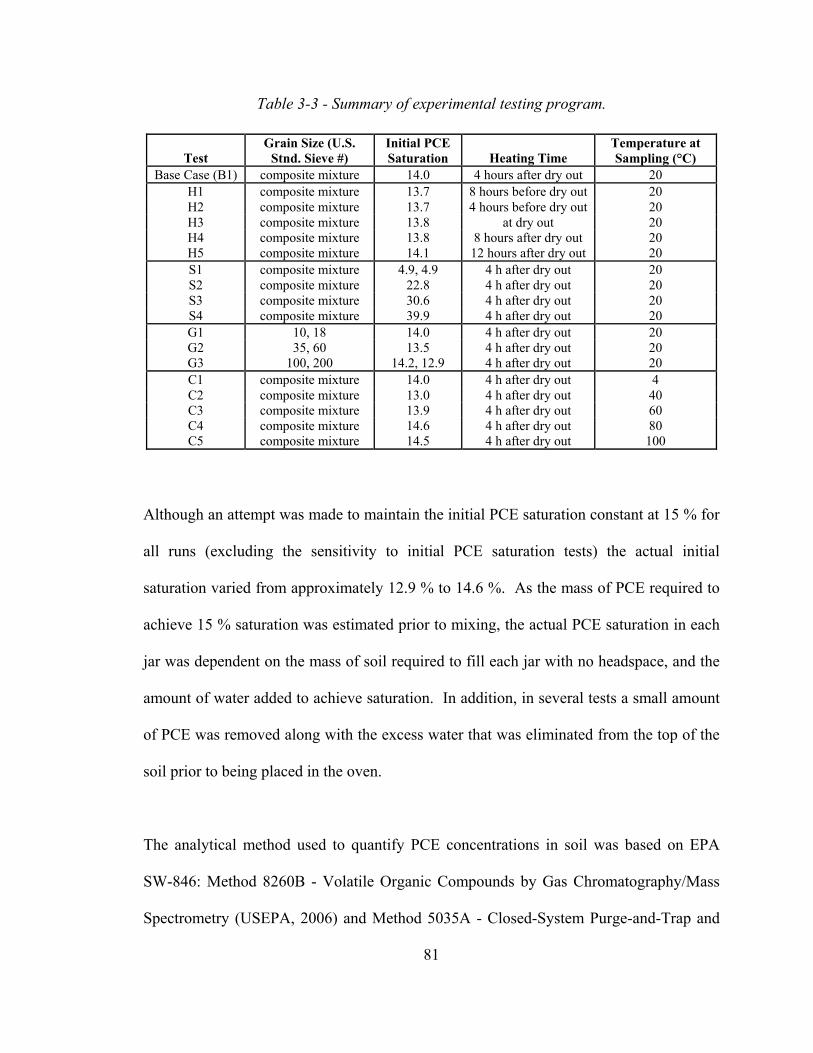
81

od 8260B - Volatile Organic Compounds by Gas Chromatography/Mass

Spectrometry (USEPA, 2006) and Method 5035A - Closed-System Purge-and-Trap and

Test Stnd. Sieve #) Saturation Heating Time Sampling (°C)

Table 3-3 - Summary of experimental testing program.

Although an attempt was made to maintain the initial PCE saturation constant at 15 % for

all runs (excluding the sensitivity to initial PCE saturation tests) the actual initial

saturation varied from approximately 12.9 % to 14.6 %. As the mass of PCE required to

achieve 15 % saturation was estimated prior to mixing, the actual PCE saturation in each

jar was dependent on the mass of soil required to fill each jar with no headspace, and the

amount of water added to achieve saturation. In addition, in several tests a small amount

of PCE was removed along with the excess water that was eliminated from the top of the

soil prior to being placed in the oven.

The analytical method used to quantify PCE concentrations in soil was based on EPA

SW-846: Meth

Grain Size (U.S. Initial PCE Temperature at

Base Case (B1) composite mixture 14.0 4 hours after dry out 20 H1 composite mixture 13.7 8 hours before dry out 20 H2 composite mixture 13.7 4 hours before dry out 20 H3 composite mixture 13.8 at dry out 20 H4 composite mixture 13.8 8 hours after dry out 20 H5 composite mixture 14.1 12 hours after dry out 20 S1 composite mixture 4.9, 4.9 4 h after dry out 20 S2 composite mixture 22.8 4 h after dry out 20 S3 composite mixture 30.6 4 h after dry out 20 S4 composite mixture 39.9 4 h after dry out 20 G1 10, 18 14.0 4 h after dry out 20 G2 35, 60 13.5 4 h after dry out 20 G3 100, 200 14.2, 12.9 4 h after dry out 20 C1 composite mixture 14.0 4 h after dry out 4 C2 composite mixture 13.0 4 h after dry out 40 C3 composite mixture 13.9 4 h after dry out 60 C4 composite mixture 14.6 4 h after dry out 80 C5 composite mixture 14.5 4 h after dry out 100

82

Extra nd Waste Samples (USEPA, 2002). A Hewlett

t of the syringe was

then spiked with surrogates fluorobenzene and deuterated 1, 4-dichloro

injection directly into the 5 ml syringe. The 5 ml sample was then immediately placed on

the purge and trap. Purging with zero-grade helium continued for 11 minutes after which

the trapped material w

desorption from the VOCARB trap. The desorbed components were then passed into the

GC where the oven temperatu

maximum of 200 ºC at a rate of 10 ºC/minute. PCE concentrations were calculated using

a 40 or 20 ppb standard solution and corrected for fluorobenzene recovery. The method

detection limit f

relative precision (coefficient of variation) of 2.6 % and 6.9 % respectively. For tests H1,

H2 and H3, the concentration of PCE in

the volume of

ater in each sample was added to the volume of methanol used in extraction. Additional

ction for Volatile Organics in Soil a

Packard 5890 Series II Plus gas chromatograph (GC) with attached Hewlett Packard

purge and trap concentrator and Hewlett Packard 5972 Series mass selective detector,

were used in the analysis. Each VOA vial was agitated aggressively for 2 minutes and

then allowed to stand until a clear layer of methanol extract was visible (see Appendix A

for photo). Using a 5 ml gas tight syringe, an aliquot of methanol extract and organic free

deionized water was taken up to form a volume of 5 ml. The conten

benzene by

as heated and back flushed with helium for 4 minutes to allow for

re was set to 65 ºC for 1 minute and then was ramped to a

or PCE in soil samples was calculated to be 2.4 ppb, with an accuracy and

post remedy samples was corrected for soil

moisture using the method outlined in Hewitt and Myers (1999) whereby

w

details on the analytical method development and statistical analysis can be found in

Appendix B.

83

3.3.2 Mathematical Model

As current post-thermal remedy soil sampling techniques involve placing hot soil cores

erature to be reached before sampling, a method

of predicting the rate of cool

analytical solution fro

distribution within a r

on ice and waiting for a desired soil temp

ing of hot cores would be an asset to many practitioners. An

m Luikov (1968) was employed to determine the temperature

finite cylinder that has been subjected to a sudden increase o

decrease in temperature on all its boundaries (i.e., heated or cooled):

( )[ ]FoKLz

RrJAA

TTTtzrT sur),,(

=−−

=Θ ∑∑∞ ∞

Lmnmn m

nmna

222

1 10

0

expcos µµµµ +−⎟⎠⎞

⎜⎝⎛

= =

(3.3)

where:

)(1 nnn J

Aµµ

= (3.4)

( )

2

m

mm µ

21+A )1(−= (3.5)

2)12( πµ −= m (3.6) m

LK L = R (3.7)

2RtFo α

= (3.8)

and µn are the roots of the Bessel function of the first kind and zero order.

The set of equations 3.3 – 3.8 form a solution to the heat diffusion equation in cylindrical

coordinates, with no temperature variation in the circumferential direction (i.e., 0=∂∂φT ),

no thermal energy generation, and no change in thermal conductivity with time:

tTzrT

zTzrT

rTzrT

RrTzrT

∂∂

=∂

∂+

∂∂

+∂

∂ ),,(1),,(),,(1),,(2

2

2

2

α (3.9)

The initial and boundary conditions are:

(3.10)

(3.11)

(3.12)

In this case, the finite cylinder’s temperature distribution is only a function of time (t),

radius (r) and z-coordinate.

Each jar containing hot soil was approximated as a finite cylinder with diameter 2R and

l

mperature is a function of time or constant) at all surfaces. The jars, initially at some

oled to Tsur = 0 ºC at all surfaces (lateral and ends), at the

initial time instant. The resultant temperature profile at the centre of the jar was

.)0,,( 0 constTzrT ==

surTtLrT =± ),,(

surTtzRT =),,(

ength 2L (Figure 3-5), with boundary conditions of the first kind (i.e., body surface

te

uniform temperature T0, were co

determined by the model and compared to the logged temperature data to estimate the

thermal diffusivity (α) of the soil.

84

85

Figure 3-5: Finite cylinder used as approximation for soil filled jar in analytical model

(adapted from Luikov, 1968).

3.4 Results and Discussion

he temperature vs. time curve for the base case test (B1) is presented in Figure 3-6. The

vapor pressure of the system. This process, also know as steam distillation occurs at

88.5 ºC for a PCE - water mixture at atmospheric pressure and continues until the

DNAPL phase PCE is depleted (Horvath, 1982). After 45 minutes, the soil temperature

again began to increase, indicating that boiling had ceased and PCE as DNAPL was no

3.4.1 Soil Temperature During Heating

T

soil temperature increased steadily from ambient to 89 ºC ± 4 ºC at which time the

temperature leveled off for approximately 45 minutes. During this time, the immiscible

mixture of PCE and water co-boiled at a temperature below the boiling point of either

individual component, as the individual vapor pressures of PCE and water sum to give the

total

86

longer present. The soil temperature leveled off at 100 ºC ± 4 ºC where boiling of the

remaining pore water continued for approximately 9 hours. After 9 hours, pore water had

been completely removed and the temperature of the soil increased until reaching a

steady-state value equal to the air temperature within the oven.

0

20

40

60

80

100

120

140

Soil

Tem

pera

ture

(ºC

)

The temperature vs. time curves for all tests followed the same trend as that displayed in

saturation was increased from 5 % to 40 % for tests S1 through S4, the duration of the co-

0 5 10 15 20Time (hours)

Figure 3-6: Soil temperature (± 4 °C) at jar center during oven heating experiment for

base case test (B1).

Figure 3-5, but with small variations in the times spent at each stage. As the initial PCE

boiling plateau increased nearly linearly from approximately 35 to 75 minutes (Figure 3-

7).

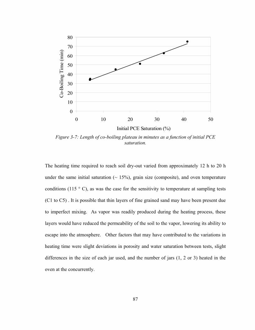
0

10

40

50

60

0 10 20 30 40 50

C-B

oilin

g T

me

(min

20

30

70

80

Initial PCE Saturation (%)

oi

)

Figure 3-7: Length of co-boiling plateau in minutes as a function of initial PCE

saturation. The heating time required to reach soil dry-out varied from approximately 12 h to 20 h

under the same initial saturation (~ 15%), grain size (composite), and oven temperature

conditions (115 ° C), as was the case for the sensitivity to temperature at sampling tests

(C1 to C5) . It is possible that thin layers of fine grained sand may have been present due

to imperfect mixing. As vapor was readily produced during the heating process, these

layers would have reduced the permeability of the soil to the vapor, lowering its ability to

scape into the atmosphere. Other factors that may have contributed to the variations in

eating time were slight deviations in porosity and water saturation between tests, slight

ifferences in the size of each jar used, and the number of jars (1, 2 or 3) heated in the

ven at the concurrently.

e

h

d

o

87

88

Results from tests H1, H2, H3, H4, H arized in Table 3-4 and shown

graphically in Figure 3-8. Error associated with the final PCE concentration

m ments is ± 6.9 %, lcula e anda ation (se ndix

B) is c down s trend exists bet heating E quantified.

The average PCE concentration declined rapidly in early sta of heating

wit he co- eau in Figur 6 wher emoved by steam

dis tio e ini 3 hour heating. The average PCE concentration

continued to decrease rapidly until the soil was dry. At soil dry-out the average soil

ncentration was 0.53 ppm. Heating for an additional 4 hours caused the PCE

oncentration to decrease to 13 ppb at which time the PCE concentration leveled off.

Once the soil has been heated for 4 hours past dry out, heating for an additional 4 and 8

hours did not affect the PCE concentration. During this time, the concentration of PCE

fluctuated between 9.0 and 19 ppb, with an average PCE concentration of 14 ppb. The

recalcitrant PCE fraction that remains may be more strongly sorbed to the soil grain

surfaces than the PCE that was removed during the boiling process. Laboratory studies

have shown that sorption of TCE to solids can be up to four orders of magnitude stronger

in an oven dried system than in a corresponding saturated system (Peterson et al., 1988).

3.4.2 Sensitivity to Heating Time

5, and are summ B1

easure as ca ted by th relative st rd devi e Appe

. It lear that a ward ween time and PC

the ges , coinciding

h t boiling plat e 3- e DNAPL was r

tilla n within th tial s of

co

c

89

Table 3-4: R oratory tests (H1 to H5) and base case test (B1).

Test Heating Saturation Time in After Heating Concentration

esults for sensitivity to heating time lab

Name Time

Initial PCE

(%) Porosity Oven (h)

Moisture Content

(wt %)

Average PCE

(ppb)

B1 after dryout 14.0 0.34 16.3 0.0 13 4 hours

H1 8 hours

before dryout 13.7 0.39 7.1 6.3 1.4 x104

H2 before dryout 13.7 0.39 11.2 4.3 7.3 x1034 hours

H3 at dryout 13.8 0.38 14.9 1.3 5.3 x102

H4 8 hours after

dryout 13.8 0.39 22.8 0.0 14

H5 dryout 14.1 0.36 26.9 0.0 15 12 hours after

1

10

100

1,000

10,000

100,000

Fil P

C C

onen

trio

n (

pb)

1,000,000

10,000,000

100,000,000

InitialConcentration

8 hours beforedryout

4 hours beforedryout

at dryout 4 hours afterdryout

8 hours afterdryout

12 hours afterdryout

Position on Heating Curve when Soil is Removed from Oven

naE

cat

p

Individual Samples

Test Average PCE

les as a function of heating time, based on

time before or after soil dry out. Figure 3-8: Concentration of PCE in soil samp

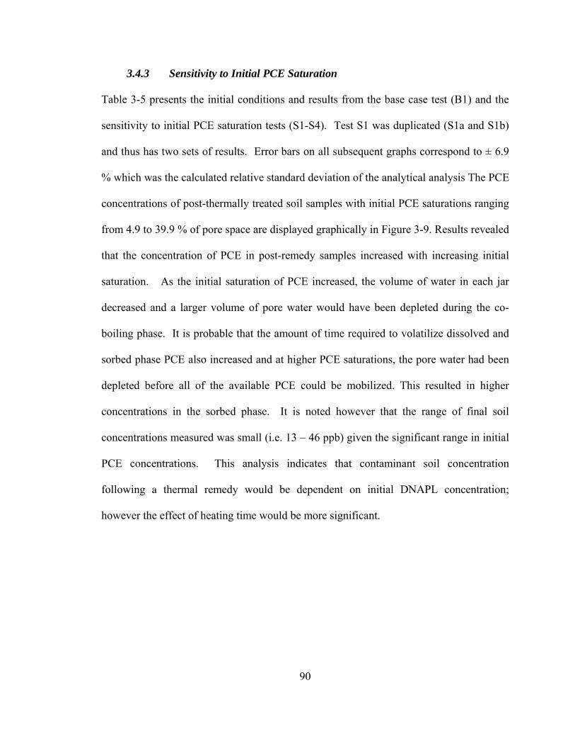
90

Table 3-5 presents the initial base case test (B1) and the

s n n 4). as d )

and thus has two sets of results. Er all graphs cor to ± 6.9

% wh as the calc relative standard deviation of the analytical analysis The PCE

concentrations of pos ally treated soil samples nitial PCE saturations ranging

from 4.9 to 39.9 % of pore space are displayed graphically in Figure 3-9. Results revealed

that the concentration of PCE in post-remedy samples increased with increasing initial

saturation. As the initial saturation of PCE increased, the volume of water in each jar

decreased and a larger volume of pore water would have been depleted during the co-

boiling phase. It is probable that the amount of time required to volatilize dissolved and

sorbed phase PCE also increased and at higher PCE saturations, the pore water had been

depleted before all of the available PCE could be mobilized. This resulted in higher

concentrations in the sorbed phase. It is noted however that the range of final soil

concentrations measured was small (i.e. 13 – 46 ppb) given the significant range in initial

PCE concentrations. This analysis indicates that contaminant soil concentration

however the effect of heating time would be more significant.

3.4.3 Sensitivity to Initial PCE Saturation

conditions and results from the

ensitivity to i itial PCE saturatio tests (S1-S Test S1 w uplicated (S1a and S1b

ror bars on subsequent respond

ich w ulated

t-therm with i

following a thermal remedy would be dependent on initial DNAPL concentration;

91

Table 3-5: Results from sensitivity to initial PCE saturation test (S1 to S4) and base case.

Test Name

Initial PCE Saturation (%)

Porosity

Time in Oven (h)

Average PCE Concentration (ppb)

B1 14.0 0.34 16.3 13 S1 a,b 4.9, 4.9 0.33, 0.36 17.4, 19.1 17, 16

S2 22.8 0.37 15.0 17 S3 30.6 0.37 15.3 23 S4 39.9 0.39 18.9 46

70

0

10

20

30

40

50

PCE

ontra

tin

(p

60

0 10 20 30 40 50Initial PCE Saturation (%)

Cce

no

pb)

Individual SamplesTest Average

Figure 3-9: Effect of initial PCE saturation (percent of pore space) on PCE quantified in

post thermally treated soil samples.

3.4.4 Sensitivity to Grain Size

Data from te n ented Table rap

3-10. Examination of these results showed a clear downward correlation between PCE

soil concentration creasing s ain size cause o trend is s the

average foc of al s for eac only va rom 0.0 (Cores 1 an – sand

sts G1, G2, G3, a d B1, are pres in 3-6 and g hically in Figure

and de and gr . The f this unclear a

l grain size h core ried f 0109 d 2

92

retained on #60 mesh) to 0.00308 (Core 3 – sand retained on #10 mesh), with no trend

with increasing or decreasing grain size apparent (see Figure 3-2). The slightly higher foc

associated with the coarse grained sand from core 3 cannot justify the significant amount

of PCE retained in the coarse soil, post-remedy. One possible explanation is that organic

matter may be a poor predictor of sorption in systems of very low foc (MacIntyre et al.,

1991). The distribution coefficient Kd (cm3/g), used to determine the ratio of equilibrium

sorbed and solution concentrations, is often calculated based on the organic carbon

content of the soil:

(3.13)

where Koc is the organic carbon partitioning coefficient (cm3/g). Equation 3.13 does not

account for sorption to minerals which may be significant in materials of low foc (Pankow

and Cherry, 1996). Piw

PCE sorption to low foc sorbents from the aqueous phase was 2 to 4 times the sorption

attrib light differences in mineralogical

Test (U.S. Standard Saturation Time in Concentration

ococd fKK =

oni and Banerjee (1989) found that the mineral phase contribution

uted to organic carbon. It is possible that s

composition between the grain size fractions could account for the phenomenon seen in

Figure 3-10.

Table 3-6: Results of sensitivity to grain size experiments.

Name

Soil Grain Size

Sieve #)

Initial PCE

(%)

Porosity Oven (h)

Average PCE

(ppb) B1 Composite 14.0 0.34 16.3 13 G1 10, 18 13.5 0.38 24.4 5.0 x102

G2 a, b 35, 60 14.2, 12.9 0.38, 0.40 23.5, 19.4 21, 30 G3 100, 200 12.0 0.40 23.7 3.4

1

10

93

100

ncen

ati

1000

0

Soil G ize (U.S . Sieve bers)

PCE

Cotr

on (p

pb)

Test AverageIndividual Samples

10,18 35,6 100,200 composite

rain S . Stnd Num

Figure 3-10: Post-thermal remedy soil PCE con tions (in al sample d test averages) unction o grain si

5 Sen ty to Tem t Sam

Results from the sensitivity to temperature at sampling tests (S1- S4) along with the base

case are presented in Table 3-7. Figure 3-11 displays graphically the effect of soil

temperature at sampling on the amount of PCE quantified in each sample. Upon visual

inspection, no obvious correlation between PCE concentration and sampling temperature

was visible. In order to confirm this observation, a Mann-Kendall trend test for multiple

observations per time period was performed on the data. For details of the Mann-Kendall

trend test analysis refer to Appendix C. The null hypothesis (H0) that no trend existed

could not be rejected therefore, this test demonstrated that soil temperature at sampling

had no effect on PCE quantified. This indicates that the fraction of PCE remaining in the

centra dividu s an as a f f sand ze.

3.4. sitivi perature a pling

94

soil after being heated for 4 hours past dry-out was sufficiently sorbed that volatilization

was no longer an effective removal mechanism. This is further confirmed by the results

of tests B1, H4 and H5 which show that the concentration of PCE in samples heated for 4,

8, and 12 hours past dry-out did not change. If no additional PCE was removed from the

soil at the oven temperature of 115 °C, it is unlikely that atmospheric exposure at any

temperature below the oven temperature would result in additional losses of PCE.

Table 3-7: Results of sensitivity to temperature at sampling tests.

Test

Name

Temperature at

Sampling (°C)

Initial PCE Saturation

(%)

Porosity Time in Oven (h)

Average PCE Concentration

(ppb) B1 20 14.0 0.34 16.3 13 C1 4 13.0 0.36 19.5 19 C2 38 13.9 0.36 21.3 29 C3 60 14.6 0.36 21.9 22C4 80 14.7 0.35 16.4 13

C5 a, b 100 14.0, 14.1 0.37, 0.37 23.9, 16.3 19, 15

95

00 20 40 60 80 100 120

Sampling Temperature (ºC)

PCE

10

20

40

60

Con

at (p

)Individual SamplesTest Average

30

50ce

ntr

ion

pb

Figure 3-11: Effect of cooling (i.e. soil temperature at sampling ± 4°C) on the amount of

.

PCE quantified in soil samples (individual samples and test averages)

3.4.6 Effect of Temperature on the Equilibrium Partitioning of PCE

The equilibrium partitioning of a chemical between the sorbed, aqueous, and gas phases

is often used as a basis for calculating the total soil concentration (CT, mg/kg) as follows

(Pankow and Cherry, 1996):

b

awwwbwdT

HCCCKCρ

φφρ ++= (3.14)

where C is the pore water concentration (mg/L), ρ is the dry soil bulk density (g/cm3), w b

φ w is the water filled porosity ([-]), H is the dimensionless Henry’s Constant, and φ a is

the air filled porosity ([-]). Equation 3.14 can be written as:

b

gwsb MMMC

ρ++

= (3.15)

where M

T

of chemical in the

ore water (C

sb is the mass of sorbed chemical (KdCwρb), Mw is the mass

wφ w), and Mg is the mass of chemical in the air phase (CwHφ ap ). In order to

As the temperature of the subsurface increases during a thermal remedy, the equilibrium

artitioning of contaminants between ph

changes in the organic carbon partitioning coefficient, aqueous solubility, and Henry’s

constant. The solubility of PCE between 21.85 and 100.85 °C was found experimentally

by Knauss et al (2000), and the Koc of PCE at varying temperatures can be estimated

through a relationship between Koc and solubility (Pankow and Cherry, 1996):

(3.16)

where c and d are empirical parameters found through regression of available data.

alues of c and d were taken from co

entally determined the distribution coefficient (Kd) of PCE at 22,

50, and 92 ºC. From the foc value given in Sleep and McClure (2001) [0.0045] and (3.13),

determine the maximum CT possible without DNAPL present, (3.14) is solved with Cw set

equal to the compound’s solubility in water (S, mg/L).

p ases varies as a result of temperature dependent

dScKoc += loglog

V rrelation analysis between Koc and S performed by

Gerstl (1990) using literature sorption data. These values for non-aromatic halogenated

compounds were -0.346 and 1.28 for c and d, respectively. It is assumed here that

Equation 3.16 is valid over the temperature range employed in this study. Sleep and

McClure (2001) experim

the percent decrease in Koc between 22 and 92 ºC was calculated to be 40.4 %. In

comparison, the Koc values predicted by (3.16) were found to decrease by 23.1 % in this

96

97

E at a reference

temperature, HR, the value can be corrected for any soil temperature using a relationship

based on the Clausius-Clapeyron/Van’t Hoff equations (USEPA, 2001):

temperature range. The reasonable agreement between Koc values predicted by (3.16) and

those determined experimentally by Sleep and McClure (2001), and the empirical nature

of (3.13) indicates that (3.16) is adequate for illustrative calculations.

With knowledge of the dimensionless Henry’s constant for PC

RT

HTTR

H

HR

Rc

vap⎥⎦

⎤⎢⎣

⎡⎟⎟⎠

⎞⎜⎜⎝

⎛−

∆−

=

11exp (3.17)

where ∆Hvap is the heat of vaporization (cal/mol) at the soil temperature of interest, T is

the soil temperature (ºK), TR is the reference soil temperature (ºK), RC is the gas constant

in cal/mol·K, and R is the gas constant in atm·m3/mol·K. The heat of vaporization in (3-

17) is calculated from published values of the heat of vaporization at the boiling point of

the contaminant ∆HvapBP (cal/mol) (USEPA, 2001):

n

Cb TT ⎦⎣ − )/1(

here T is the critical temperature (ºK), T is the boiling point (ºK) and n is a unitless

CvapBPvap

TTHH ⎥⎤

⎢⎡ −

∆=∆)/1( (3.18)

C b

Tb/TC (n = 0.3, for this case). For PCE the ∆Hvap at

121.25 ºC is 8,288 cal/mol (Lide, 2003) Further details of these calculations are provided

w

exponent that is dependent on the ratio

in Appendix E.

For PCE within the temperature range of 21.85 °C to 100.85 °C the percentage

distribution of PCE mass among the phases is shown in Figure 3-12. The relationship

98

.2 and foc of 0.0016 were used to

calculate the trends shown in Figure 3-12. The dramatic increase in CT indicates that at

temperatures characteristic of thermal remediation processes, much higher concentrations

of PCE can exists in the subsurface without the presence of DNAPL.

between CT and increasing temperature is also shown. A soil dry bulk density of 1.86

g/cm3, air filled porosity of 0.1, water filled porosity of 0

0

10

P

50

Max

i

20

30

40

50

60

70

80

0 20 40 60 80 100 120

erce

ntag

e of

Tot

al M

ass (

%)

0

100

150

200

250

300

350

400

450

500

mum

PC

E C

once

ntra

tion

(CT)

(mg/

kg)

Temperature (°C)

AqueousSorbedGasCT

T

process. The initial temperature (T0) was the soil temperature when each jar was

rst immersed in the ice bath. Results of the base case test (B1) are displayed in Figure

Figure 3-12: Percentage of PCE mass in aqueous, gas, sorbed, and gas phases and maximum PCE concentration without the presence of NAPL (C ) at varying temperature.

3.4.7 Mathematical Model

In order to determine the thermal diffusivity (α) of the soil used in each test, solutions of

the analytical model were fit to the experimentally recorded soil temperature during the

cooling

fi

3-13. From visual inspection, the thermal diffusivity of the sand used in test B1 was

between approximately 1.65 x 10-7and 1.55 x 10-7 m2/s.

0

120

99

20

40

60

0 20 40 60 80 100 120

Tm

pur

e

80

100

Time (minutes)

eer

at (º

Experimental Data B1

C)

α = 1.4e-7 m^2/sα = 1.5e-7 m^2/sα = 1.6e-7 m^2/sα = 1.7e-7 m^2/s

l diffusivities at later

time.

Figure 3-13: Soil temperature (± 4 °C ) at jar centre during cooling from experimental

data and as derived by analytical model.

The experimental temperature data fit the analytical model well for the sensitivity to

initial PCE saturation tests (S1-S4) and sensitivity to cooling time tests (C1-C5). The

thermal diffusivity of these soils ranged from 1.4 x 10-7 at early cooling time to 1.8 x 10-7

m2/s at late time. All tests followed a similar trend whereby a temperature profile

characteristic of higher thermal diffusivities was observed at early cooling time and

followed by a temperature profile characteristic of lower therma

100

The thermal diffusivity of the sand used in tests G1 (coarse grained sand), G2 (medium

grained sand), and G3 (fine grained sand) as calculated by the analytical model were

within the same range as seen in the previous tests (i.e., between 1.4 x 10-7 at early time

and 1.6 x 10-7 m2/s at late time). No correlation between grain size and thermal

diffusivity was observed.

The cooling temperature profiles from tests H1 and H2 deviated from those observed in

other tests. For other tests, the soil temperature at the centre of each jar remained

constant for a period of time following placement in the ice bath. Due to its heat

capacity, the soil maintains its thermal energy while the cooling front propagates from

o

r dr the

ignificant moisture content that remained in the samples after heating. In test H1 and H2

utsides of the jar to the centre. In tests H1 and H2, the temperature in the centre of each

opped soon after placement in the ice bath (see Figure 3-14). This was a result of

ja

s

the soil was removed from the oven before dry-out and during pore water boiling. As the

pore water boiled, a portion of the produced water vapor likely became trapped in the

porous medium and condensed as the cooling front propagated through the jars. The

analytical model does not account for phase change (condensation of water vapor) which

provides a distinct set of initial conditions from those characteristic of simple conductive

cooling. It can be noted that although the initial temperature drops observed in tests H1

and H2 were not predicted by the model, the slopes of the temperature profiles at later

time were similar to the curves calculated by the analytical model.

101

0

20

60

0 20 40 60 80 100 120Time (minutes)

emp

ratu

40

100

120

Te

80C)re

(ºExperimental Data H1α = 1.3e-7m^2/sα = 1.6e-7m^2/sα = 1.8e-7m^2/sExperimental Data H2

ture ( ± 4 °C) at jar centre during cooling in ice bath for test H1

and H2, as compared with temperature profiles generated by analytical model.

Discrepancies between the temperature profiles predicted by the analytical model and the

temperature profiles from experimental data for the dry sand samples are the result of

variations between the ideal system used in the model and the actual experimental

conditions. However, the model accurately predicts the shape of the cooling profile and

the early and late time α values are within a narrow range (± approximately 2 x 10 m /s).

In addition, the range of thermal diffusivities found through fit with the analytical model

agree well with many literature and experimental values. Chirdon et al. (2007) found the

α of dry concrete sand to be 1.7 x 10 m /s, while Bejan and Kraus (2003) published 1.6

x 10 m /s as the thermal diffusivity of coarse grained earth material. It is clear that the

Figure 3-14: Tempera

-8 2

-7 2

-7 2

102

ntil DNAPL was depleted. An increasing linear correlation was found between

itial PCE saturation and the length of the co-boiling plateau. After DNAPL was

perature increased to 100 ºC ± 4 ºC where boiling of the remaining

pore water continued.

Results from the sensitivity to heating time tests indicated that most DANPL was

depleted during the early stages of heating, coinciding with co-boiling of the pore water-

PCE mixture at a temperature below the boiling point of water. Once the soil had been

heated past dry-out, the concentration of PCE remaining in the soil did not decrease upon

further heating. Increasing the value of initial PCE saturation resulted in slight increases

in the final concentration of residual PCE. This effect was found to be slight in

comparison to the large ranges in initial saturations examined. A decreasing trend was

found between decreasing grain size and the final amount of PCE quantified.

Temperature at sampling was not found to affect the concentration of PCE in post-

thermal remedy samples under the selected experimental conditions.

rate of cooling within a soil core can be reasonably predicted using the employed

analytical solution.

3.5 Conclusions

A soil temperature profile during heating was created which clearly depicts a co- boiling

plateau. After steadily increasing from ambient temperature to 89 ºC ± 4 ºC, the soil

temperature leveled off where PCE and water formed an immiscible mixture which co-

boiled u

in

depleted, the soil tem

103

he cylindrical heat diffusion equation was modeled to produce a

mperature profile at the centre of each jar during the cooling process. Experimental

thermal

initia icate that the

an ice

bath.

An analytical solution of t

te

cooling data was fit to the curves predicted by the model in order to estimate the

diffusivity of the soil. The thermal diffusivity of the dry sand used in the laboratory study

was found to range from 1.4 x 10-7 to 1.8 x 10-7 m2/s. No trend between grain size or

l PCE saturation and thermal diffusivity was observed. Results ind

model is applicable for predicting the rate of cooling of a hot soil core placed in

104

ASTM, 2006. Standard Guide for Sampling Waste and Soils for Volatile Organic Compounds. American Society for Testing and Materials, D 4547-06.

Bejan, A., Kraus, A. D., 2003. Heat Transfer Handbook. John Wiley & Sons, New York.

Hydrating Portland Cement Mortars Using an Oscillating Boundary Temperature. Cement and Concrete Research 37, 680-690.

Davi

/540/S-97/502.

ings of the Third International Conference on Remediation of Chlorinated and Recalcitrant Compounds, 307-310.

Gerst rption by Soils. Journal of Contaminant Hydrology 6, 457-375.

Hansrnational Symposium on

Environmental Biotechnologies and Site Remediation Technologies, Orlando,

Heron, G., Christensen, T.H., Enfield, C.G., 1998. Henry’s Law Constant for

Trichloroethylene between 10 and 95°C. Environ. Sci. Technol. 32, 1433-1437.

Heroesistance Heating. Ground

Water Monitoring and Remediation 25 (4), 92 – 107.

Hewin Soil and Groundwater. US Army Corps of Engineers. Special Report

99-16.

Horv cel Dekker, Inc., NY.


Chirdon, W.M., Aquino, W., Hover, K.C., 2007. A Method for Measuring Transient

Thermal Diffusivity in

s, E.L., 1997. How Heat Can Enhance In-Situ Soil and Aquifer Remediation: Important Chemical Properties and Guidance on Choosing the Appropriate Technique. EPA: Groundwater Issue; EPA

Gaberell, M., Gavaskar, A., Drescher, E., Sminchak, J., Cumming, L., Yoon, W., De

Silva, S., 2002. Soil Core Characterization Strategy at DNAPL Sites Subjected to Strong Thermal or Chemical Remediation. Proceed

l, Z., 1990. Estimation of Organic Chemical So

en, K. S., and Conley, D. M., Vinegar, H.J., Coles, J.M., Menotti, J.L., Stegemeier, G.L., 1998. In Situ Thermal Desorption of Coal Tar. Inte

Florida, December 7-9, 1998.

n, G., Carroll, S., Nielsen, S.G., 2005. Full-Scale Removal of DNAPL Constituents Using Steam-Enhanced Extraction and Electrical R

tt A.D., and Myers, K.F., 1999. Sampling and On-Site Analytical Methods for Volatiles i

ath, A. L., 1982. Halogenated Hydrocarbons, Solubility-Miscibility with Water. Mar

105

Steam Injection. American Society of Mechanical Engineers, Fluids Engineering Division, FED 173,

Lide, C Handbook of Chemistry and Physics 84/e., CRC Press, Boca

Raton, FL,

Luiko

aslusky, S.F., and Udell, K.S., 2005. Co-injection of Air and Steam for the Prevention

tio Predictions. Journal of Contaminant Hydrology 77 (4), 325-347.

Knau

rature. Applied Geochemistry 15, 501-512

: Pump-and-Treat

acIntyre, W.G., Stauffer, T.B., and Antworth, C.P., 1991. A Comparison of Sorption

ankow, J.F., and Cherry, J.A., 1996. Dense Chlorinated Solvents and other DNAPLs in

tland,

eterson, M.S., Lion, L.W., Shoemaker, C.A., 1988. Influence of Vapor-Phase Sorption

.

iwoni, M.D., and Banerjee, P., 1989. Sorption of Volatile Organic Solvents from

Aqueous Solution onto Subsurface Solids. Journal of Contaminant Hydrology 4, 163-179.

She, H.Y. and Sleep, B.E., 1999. Removal of Perchloroethylene from a Layered Soil

System by Steam Flushing. Ground Water Monitoring and Remediation 19 (2), 70-77.

Sleep, B.E., and McClure, P.D., 2001a. Removal of Volatile and Semivolatile Organic

Contamination from Soil and Air by Steam Flushing. Journal of Contaminant Hydrology 50, 21-40.

Itamura, M.T., and Udell, K.S., 1993. Experimental Clean-up of a Dense Non-Aqueous Liquid in the Unsaturated Zone of a Porous Medium Using

57-62.

D.R., ed., 2003. CR

v, A.V., Hartnett, J.P, (ed.), 1968. Analytical Heat Diffusion Theory. Academic Press, New York, NY.

Kof the Downward Migration of DNAPLs during Steam Enhanced Extraction: An Experimental Evaluation of Optimum Injection Ra

ss, K.G., Dibley, M.J., Lerif, R.N., Mew, D.A., Aines, R.D., 2000. The Aqueous Solubility of Trichloroethylene (TCE) and Tetrachloroethylene (PCE) as a Function of Tempe

Mackay, D.M., and Cherry, J.A., 1989. Groundwater Contamination

Remediation. Environ. Sci. Technol. 23 (6), 630-636

MCoefficients Determined by Batch, Column, and Box methods on a Low OrganicCarbon Aquifer Material. Ground Water 29 (6), 908-913.

PGroundwater: History, Behavior, and Remediation. Waterloo Press, PorOregon, 1996.

Pand Diffusion on the Fate of Trichloroethylene in an Unsaturated Aquifer SystemEnvironmental Science and Technology 22, 571-578.

P

106

Sleep, B.E. and McClure, P.D., 200 t of Temperature on Adsorption of Organic Compounds to Soils. Can. Geotech. J. 38, 46-52.

Siegrist, R.L., Jenssen, P.D., 1990.

Organic Compo . Sci. Technol. 24 (9), 1387-1392.

r , K.S., Crimi, M.L., Urynowicz, M.A., 2006. Quantifying PCE and TCE in DNAPL Source Zones: Effects of Sampling Methods Used for Intact Cores

1b. The Effec

Evaluation of Sampling Method Effects on Volatile und Measurements in Contaminated Soils. Environ

Sieg ist, R.L., Lowe

at Varied Contaminant Levels and Media Temperatures. Ground Water Monitoring & Remediation 26 (2), 114-124.

Smart, J.L., 2005. Application of Six-Phase Soil Heating Technology for Groundwater

Remediation. Environmental Progress 24 (1), 34-43. Stegemeier, G.L., and Vinegar, H. J., 2001. Thermal Conduction Heating for In-Situ

Thermal Desorption of Soils. In Oh, Chang H. (ed), Hazardous & Radioactive Waste Treatment Technologies Handbook, Chapter 4.6-1. CRC Press, Boca Raton, Florida.

USEPA, 1996. Method 8260B – Volatile Organic Compounds by Gas

Chromatography/Mass Spectrometry (GC/MS). EPA Test Methods, SW-846. [Online] http://www.epa.gov/epaoswer/hazwaste/test/pdfs/8260b.pdf

USEPA, 2001. Fact Sheet - Correcting the Henry’s Law Constant for Soil Temperature.

EPA Online Tools for Site Assessment Calculation. [Online] http://www.epa.gov/AthensR/learn2model/part-two/onsite/doc/factsheet.pdf

USEPA, 2002. Method 5035A - Closed-System Purge-and-Trap and Extraction for Volatile Organics in Soil and Waste Samples. EPA Test Methods, SW-846. [Online] http://www.epa.gov/epaoswer/hazwaste/test/pdfs/5035a_r1.pdf

Udell, K.S., 1996. Heat and Mass Transfer in Clean-up of Underground Toxic Wastes. In: Chang-Lin Tien (ed.), Annual Review of Heat Transfer. BYork, Wallingford, UK, p 333-405.

egell House, Inc.: New

107

4.1

emperature data collected at the centre of each jar during heating showed a steady

und between initial

CE saturation within the jar and the length of the co-boiling plateau. Once DNAPL PCE

water or of the contaminant do not have to be

Chapter 4

CONCLUSIONS AND RECOMMENDATIONS

Conclusions

T

increase in soil temperature from ambient to 89 ºC ∀ 4 ºC where the soil temperature

reached a plateau that was maintained for approximately 35 – 75 minutes. During this

time, dense non-aqueous phase liquid (DNAPL) tetrachlroethylene (PCE) and the soil

pore water formed an immiscible mixture that underwent co-boiling until the DNAPL

phase PCE was depleted. An increasing linear relationship was fo

P

had been depleted, the soil temperature again increased until leveling off at 100 ºC ∀ 4

ºC at which point the remaining pore water began to boil. The soil temperature remained

constant until all pore water had been depleted, after which the temperature again

increased until reaching equilibrium with the temperature within the oven. These results

demonstrated that the boiling point of

reached for in-situ boiling and depletion of DNAPL to occur.

Of the variables examined, heating time was found to have the most significant effect on

the concentration of PCE in post-remedy samples. Coinciding with the co-boiling

plateau observed in temperature vs. time curves, the sensitivity of final PCE

concentration to heating time tests showed that approximately 70 % of DNAPL mass was

108

NAPL phase PCE by heating only to the end of co-

oiling plateau may be sufficient for achieving the remediation goals.

re

t sampling tests showed no trend. This leads to the conclusion that cooling of soil cores

st dry-out is not necessary to achieve accurate post-thermal

edy concentration measurements.

Analysis of the partitioning of volatile organic compounds (VOCs) such as PCE as a

function of temperature indicated that the percentage of the total PCE mass in the

aqueous and sorbed phases declines from 67.84 to 13.46 % and from 24.29 to 8.54 %,

respectively, between 21.85 and 123.85 ºC, while the concentration in the gas phase

increases from 7.88 to 78.00 %. As gas phase recovery is the primary removal

removed during the initial 4 - 5 hours of heating (8 hours before soil dry-out). Soil PCE

concentration continued to decline until after soil dry-out, after which, heating for an

additional 4 to 8 hours did not result in a further decline in PCE concentration. For many

field applications, depletion of D

b

Increasing initial PCE saturation resulted in slight increases in final PCE concentrations.

The range in final PCE concentrations quantified was small in relation to the large

variations in initial PCE saturations analyzed. This indicates that the initial saturation of

DNAPL at an impacted site would have little or no relation to the final concentration,

post-thermal remedy, if the subsurface is to be heated past dry-out.

Sensitivity to soil grain size laboratory tests showed that the amount of PCE quantified

post-remedy increased with increasing sand grain size, while, sensitivity to temperatu

a

that have been heated pa

rem

mechanism of many remediation techniques, the results of this analysis indicate that

temperatures customary of thermal remediation techniques effectively increase the

obility and recovery of contaminants, in comparison to techniques that operate at

ous

aterial with uniform thermal properties. The rate of cooling predicted is less accurate

In future studies, development of a method to ensure that the initial porosity and moisture

content of each jar are completely consistent between each test would be useful.

Although the method used resulted in a relatively narrow range of measured porosities

(between 0.33 and 0.40), further reducing this range would result in a greater degree of

accuracy as the number of variables that may affect the final concentration of PCE are

reduced. A revised method of spiking and saturating the soil to ensure a uniform

m

ambient temperature conditions.

An analytical solution of the conductive heat equation in cylindrical coordinates has been

found to accurately predict the rate of cooling of a hot soil core that has been placed on

ice. This is interesting as the model assumes that the jar containing soil is a homogene

m

when the soil pore water had been undergoing boiling when it was suddenly immersed in

ice. This is most likely due to trapped vapours undergoing condensation, as the model

does not account for the conditions present during phase change. The thermal diffusivity

of the sand used in the heating experiments, as predicted through fitting of the model

with experimental temperature data, was found to coincide well with literature values.

4.2 Recommendations

109

distribution of PCE and com ful in order to decrease the

variability of initial conditions between each run.

Inform ld

be of in us

locatio thi ed

in ther in

which the f ne soil p ixture.

The ef his

study a ed mpact soil ad

been h en

E

wn

the

wide the

effec eatin t a hat p the

conce oil

hydra

plete saturation would also be use

ation on the temperature profile within each jar during the heating process wou

terest. This could be accomplished by using an array of thermocouples at vario

ns wi n each jar. In order to better understand the mechanisms that are involv

mal remediation at an impacted field site, further experimentation is needed

i articles (clay and silt) are included in the soil grain size m

fect of cooling on post-thermal remedy samples should be studied further. T

nalyz the sensitivity to temperature at sampling for PCE i ed that h

eated past dry-out. Future work on the effect of cooling on soil that had be

heated for shorter periods of time (i.e., before dry-out), spiked with various initial PC

saturations, and soil of varying grain sizes would be valuable. In this study it was sho

that the range of final PCE concentrations measured was narrow in comparison to

range of initial PCE saturations analyzed. It would be interesting to determine

t of h g time for each of these initial saturations and to find ou t w oint

ntrations became relatively equivalent. The impact, if any, of keeping the s

ted during the heating process would also be of interest.

110

Appendices – Contents

Appendix A – Experimental Data, Observations, and Calculations 120

A.1 Soil Core Boring Log 121

A.2 Particle Size Analysis 122

A.3 Fraction Organic Carbon (foc) Measurements 134

A.4 Determination of Individual Grain Size Masses in Composite Mixture 137

A.5 Calculation of Porosity and PCE Saturation of Soil Prior to Heating 138

A.6 Analytical Results 140

A.7 Soil Temperature vs. Time during Heating Graphs 143

A.8 Selected Laboratory Photographs 154

A.9 Literature Cited 158

Appendix B – Analytical Method 159

B.1 Methodology 160

B.2 Calibration and Standards 162

B.3 Quality Control, Quality Assurance, and Error Analysis 163

B.3.1 Statistical Theory 164

B.3.2 Propagation of Error 165

B.3.3 Method Detection Limit 166

B.3.4 Analytical Method Error 166

B.4 Literature Cited 170

Appendix C – Mann-Kendall Trend Test 171

C.1 Methodology 172

111

C.2 Results 174

C.3 Literature Cited 176

Appendix D – Mathematical Model 177

D.1 Background 178

D.2 Model Verification 180

.3 Results of Analytical Model – Fitting to Ex er D p imental Data 183

D.4 Example MATLAB Code 194

D.5 Literature Cited 196

Appendix E – Properties of PCE as a Funct T r ion of empe ature 197

E.1 Henry’s Constant 198

.2 Vapor Pressure 201 E

E.3 Solubility 203

E effici nt (Koc .4 Organic Carbon Partitioning Co e ) 204

.5 Literature Cited 205 E

112

Appendices – List of Tables

A-1 Soil boring log for core 1 (3.048 - 4.572 m bgs) 121

A-2 Soil boring log for core 2 (4.572 - 6.096 m bgs) 122

A-3 Soil boring log for core 3 (6.096 – 7.620 m bgs) 123

4 - Soil boring log for core 4 (7.620 – 9.144 m bgs) 123 A

-5 Results of sieve analysis for core 1. 125 A

Results of hydrometer analysis for core 1. 126 A-6

A-7 Results of sieve analysis for core 2. 127 A-8 Results of hydrometer analysis for core 2. 128 A-9 Results of sieve analysis for core 3. 129 A-10 Results of hydrometer analysis for core 3. 130 A-11 Results of sieve analysis for core 4. 131 A-12 Results of hydrometer analysis for core 4. 132 A-13 Results of foc analysis for each core segment. a “composite” refers to a

mixture containing all grain sizes, b “1 & 2” denotes a mixture of soil from core segments 1 and 2. 134

A-14 Data used for calculation of mass of each grain size in 1 kg composite sample. 137 A-15 Analytical results for PCE concentration in each soil sample for base case (B1) and sensitivity to heating time tests (H1-H5). 140 A-16 Analytical results for PCE concentration in each soil sample sensitivity to initial PCE saturation tests (S1-S4). 141 A-17 Analytical results for PCE concentration in each soil sample for sensitivity to grain size tests (G1-G3). 141 A-18 Analytical results for PCE concentration in each soil sample for sensitivity to temperature at sampling tests (C1-C5). 142

113

B-1 Results of 5 spi f the method detection limit (MDL).

ked soil samples used for determination o 166

B-2 Results of 5 spiked soil samples used for calculation of accuracy and precision of analytical method. 167 B-3 Example calculation for measurement error in analytical method. 168 C-1 Mann-Kendall trend test for sensitivity to temperature at sampling data (tests C1-C5) and base case (B1). 173 C-2 Key parameters calculated in Mann-Kendall trend analysis. 175 E-1 Data used in calculation of dime o c t E nsi nless Henry’s onstan of PC as a

function of temperature. 199 E-2 Vapor pressure of PCE as a function of temperature c la om alcu ted fr the

Antoine Equation. 201

114

Appendices – List of Figures

A-1 Grain size distribution curve for core 1. 127

2

- Grain size distribution curve for core 2. A 129



5

- Soil temperature (± 4 °C) at the centre of jar for base case test as a function A

of heating time (time in oven). 143

6

- Soil temperature (± 4 °C) at the centre of jar for sensitivity to heating time A

test H1 as a function of heating time (time in oven). 144

7

- Soil temperature (± 4 °C) at the centre of jar for sensitivity to heating time A

test H2 as a function of heating time (time in oven). 144

8

- Soil temperature (± 4 °C) at the centre of jar for sensitivity to heating time A test H3 as a function of heating time (time in oven). 145

9

- Soil temperature (± 4 °C) at the centre of jar for sensitivity to heating time A test H4 as a function of heating time (time in oven). 145

10

- Soil temperature (± 4 °C) at the centre of jar for sensitivity to heating time A test H5 as a function of heating time (time in oven). 146 A-11 Soil temperature (± 4 °C) at the centre of jar for sensitivity to initial PCE

saturation test S1a as a function of heating time (time in oven). 146

-12 Soil temperature (± 4 °C) at the centre of jar for sensitivity to initial PCE Asaturation test S1b as a function of heating time (time in oven). 147

-13 Soil temperature (± 4 °C) at the centre of jar for sensitivity to initial PCE A

saturation test S2 as a function of heating time (time in oven). 147

14 jar for se

- Soil temperature (± 4 °C) at the centre of nsitivity to initial PCE Asaturation test S3 as a function of heating time (time in oven). 148

ov n).

-15 Soil temperature (± 4 °C) at the centre of jar for sensitivity to initial PCE A

saturation test S4 as a function of heating time (time in e 148 A-16 Soil temperature (± 4 °C) at the centre of jar for sensitivity to grain size

oven). test G1 as a function of heating time (time in 149

115

A-17 Soil temperature (± 4 °C) at the centre of jar for sensitivity to grain size

test G2a as a function of heating time (time in oven). 149

-18 Soil temperature (± 4 °C) at the centre of jar for sensitivity to grain size A test G2b as a function of heating time (time in oven). 150

-19 Soil temperature (± 4 °C) at the centre of jar for sensitivity to grain size A test G3 as a function of heating time (time in oven). 150

-20 Soil temperature (± 4 °C) at the centre of jar for sensitivity to temperature A at sampling test C1 as a function of heating time (time in oven). 151




Soil temperature (± 4 °C) at the centre of jar for sensitivity to temperature A-24

at sampling test C5a as a function of heating time (time in oven). 153

A-25 perature

Soil temperature (± 4 °C) at the centre of jar for sensitivity to temat sampling test C5b as a function of heating time (time in oven). 153

A-26 Soil core segments in outer casing upon receipt in laboratory. 154

Soil core segment #2 in PVC tubing with outer casing removed. 154 A-27

A-28 Jar filled with saturated soil aggregate and PCE-DNAPL. 155 A-29

in centre. Filled open jars placed in oven for heating with thermocouple probes

155

A-30

Jar cap with thermocouple probe through centre for temperature measurement during cooling in ice bath. 156

A-31 Soil filled jar in ice bath for cooling with thermocouple probe for

temperature measurement. 156

-32 Soil sampling with Terra Core Sampler after cooling. A 157

A-33 5 g soil sample after methanol extraction with clear layer of methanol

above soil for injection into purge-and-trap. 157

116

Calibration curve for purge-and-trap GC/MS used for analytical analysis.

B-1 163

D-1 Finite Cylinder Used for Approximation of Soil Filled Jars (adapted from

Luikov, 1968). 179

-2 Dimensionless temperature vs. increasing values of ‘n’ as solved by Danalytical model. 181

D-3

nalytical model. Dimensionless temperature vs. increasing values of ‘m’ as solved by a 182

D-4

Temperature at Disk Centre as a Function of Time for model verification, based on example from Luikov (1969), pg. 165. 182

D-5 Soil temperature (± 4 °C) at jar centre during cooling for base case test (B1):

experimental data and temperatures predicted by analytical model. 183

-6 Soil temperature (± 4 °C) at jar centre during cooling for sensitivity to heating Dtime tests H1 and H2: experimental data and temperatures predicted by analytical model. 184

-7 Soil temperature (± 4 °C) at jar centre during cooling for sensitivity to heating D

time test H3: experimental data and temperatures predicted by analytical model. 184

-8: Soil temperature (± 4 °C) at jar centre during cooling for sensitivity to heating D

time test H4: experimental data and temperatures predicted by analytical model. 185

-9 Soil temperature (± 4 °C) at jar centre during cooling for sensitivity to D

heating time test H5: experimental data and temperatures predicted by analytical model. 185

-10 Soil temperature (± 4 °C) at jar centre during cooling for sensitivity to initial

y D

PCE saturation test S1a: experimental data and temperatures predicted banalytical model. 186

-11 Soil temperature (± 4 °C ) at jar centre during cooling for sensitivity to initial

by D

PCE saturation test S1b: experimental data and temperatures predicted analytical model. 186

-12 Soil temperature (± 4 °C) at jar centre during cooling for sensitivity to initial

PCE saturation test S2: experimental data and temperatures predicted by analytical model.

D

187

117

Soil temperature (± 4 °C) at jar centre during cooling for sensitivity to inD-13 itial

nalytical model. PCE saturation test S3: experimental data and temperatures predicted by a 187

D-14 CE saturation test S4: experimental data and temperatures predicted by

Soil temperature (± 4 °C) at jar centre during cooling for sensitivity to initial Panalytical model. 188

-15 Soil temperature (± 4 °C) at jar centre during cooling for sensitivity to

d by D

grain size test G1: experimental data and temperatures predicteanalytical model. 188

ivity to grain

model.

D-16 Soil temperature (± 4 °C) at jar centre during cooling for sensitsize test G2a: experimental data and temperatures predicted by analytical

189

D-17 Soil temperature (± 4 °C) at jar cen during cooling for sensitivity to grain size test G2b: experimental da peratures predicted by analytical model.

treta and tem

189 D-18 Soil temperature (± 4 °C) at jar centre during cooling for sensitivity to

grain size test G3: experimental data and temperatures predicted by analytical model. 190

D-19 Soil temperature (± 4 °C) at jar cen during cooling for sensitivity to

temperature at sampling test C1: experimental data and temperatures predicted by analytical model.

tre

190 D-20 Soil temperature (± 4 °C) at jar centre during cooling for sensitivity to

temperature at sampling test C2: ex rimental data and temperatures predicted by analytical model.

pe 191



trepe 191

D-22 Soil temperature (± 4 °C) at jar centre during cooling for sensitivity to


pe 192


temperature at sampling test C5a: experimental data and temperatures predicted by analytical model.

tre

193

118

D-24 Soil temperature (± 4 °C) at jar cen during cooling for sensitivity to temperature at sampling test C5b: experimental data and temperatures predicted by analytical model.

tre

193

E-1 Dimensionless Henry’s constant for PCE as a function of temperature between 0°C and 110 °C. 200

E-2 Vapor pressure of PCE as a function of temperature as calculated from the Antoine Equation. 202

E-3 Solubility of PCE as a function of temperature (adapted from

Knauss et al., 2000). 203 E-4 Organic carbon partitioning coefficient for PCE as a function

of temperature. 204

119

Appendix A

EXP OB

ERIMENTAL DATA, SERVATIONS &

CALCULATIONS

120

A.1 Soil Core

Upon receipt, each 5 ft soil core was cut lengthwise and opened in order to record a soil

borin . The obser the examina are

presented in Tables A-1 through A-4.

)

Distance fro f Core (cm) General Description

Boring Log

g log vations made during tion of each core segment

Table A-1: Soil boring log for core 1 (3.048 - 4.572 m bgs

m Top oUnique Features of Section

0-51 - massive, uniform sand - possible till

- poorly graded - orange/brown in color - no visible layers

- few small cobbles (<2cm in diameter)

54-108 - visible, alternating, thin (<3mm) layers

-c large boulder @ 54cm (6 x 5 x 4 m)

of light colored sand and dark coloredsilt/clay

- high percentage of fines (>50%), - cluster of cobbles @ 68-74cm with

diameters ranging from 1-2 cm less sand

- evidence of drilling around sides core, layers curve downwards tow

of ards

dges - cobbles are equant, pitted, and angular e

- some dark mineral material present in thin layers

- dark shiny specks @ 102-110cm

111-132 - possible till - many cobbles of varying sizes

- large boulder present @ 111cm : dimensions are 7 x 4 x 3 cm

- poorly graded sand - location of possible biotite @ 128cm - light grey/brown colored - thin orange layer @ 130-132cm

135-152 - well-graded sand - collection of cobbles @145-148cm

- light grey/brown colored with few lighter colored areas

- most stones are angular, equant and pitted

- overall, very uniform - large boulder with length = 7cm

121

Table A-2: Soil boring log for core 2 (4.572 - 6.096 m bgs)

Distance from

Top of Core escription (cm) General D Unique Features of Section

0-18 - possible till - poorly graded sand - some layers visible @18-51cm

olor - orange/brown c

- few dispersed cobbles which are sub-angular

- soil is moist, and very hard

21-117 , and

- coarse sand

- alternating dark grey and orange in color (most likely sandclay/silt)

- soil is a darker, grayish in color - large sub-angular boulder present @ 20cm (5 x 3 x 8 cm)

- lighter color between 30-47cm in a line down through the centre of the

- slightly softer than @ 0-18cm core - boulder present @ 35cm

- large sub-rounded boulder present @ 118-123cm

1 2 - finer sand than throughout rest of

ass @ 152-153cm 20-15 core - orange m compacted) - soil is very hard (

ge that from 18-

- color is more oran117cm

section - many cobbles present in this - some layers visible (alternating orange and grey), ~ 2-3mm thick

122

Table A-3: Soil boring log for core 3 (6.096 – 7.620 m bgs)

(cm) General Description Unique Features of Section

Distance from Top of Core

0-91 - possible outwash

- orangey/brown in color

- segment is much more homogenous

- no visible layering

- many large stones visible @ 0-

- cohesive sandy layer @ 30cm

- orangey spot along edge of core

- dark spot @ 62 – 63 cm

- moist and cohesive

- water is visible

that segments 1 or 2

30cm

- sandy clay between 30- 36 cm

between 37 and 43 cm

91-152 - soil is very dry - grey in color - evidence of drilling along edges

- soil in centre of core is especially dry and non-cohesive - crumbles very easily

Table A-4: Soil boring log for core 4 (7.620 – 9.144 m bgs)

Distance from Top of Core

(cm) General Description Unique Features of Section 0-15 - overall, core is more homogenous than

previous segments - possible outwash

- high percentage of clay

- very red in color - some brown soil around side

15-54 - alternating red and grayish layers - grey layers are more sandy

54-152 - mixed red sand and grey clay

sides of core

- large coble @ 63-70 cm - evidence of drilling - red layer along

- no visible lamina

- large coble @ 117-124 cm

123

124

re) in order to separate the fine particles (clay and silt)

the coarse particles (sand, gravel, cobles). The separated soil particles were then

oven dried to obtain dry

a #4 (4.75 mm aperture) sieve to separate gravel from sand particles. Recovered sand

pa c then p hrou s

#60, #100, and #200) in order to determ s

passed through six sieves with m es ran from 6.3 to 50 mm.

represen ive samples of fine particles from each segments were analyzed by the

hydrom method to ine the ze distri n of the and silt fractions.

Results of the sieve and hydrometer analysis for core segment #1 are shown in Table A-5

and Table A-6 and the grain size distribution curve for core segment 1 is displayed in

Figure A-1. In Table A-5, m s fers to e mass of soil that does ot pass

thr ugh the sieve ained he percentage of the to

egment that does not pass through the sieve, while the cumulative percentage retained

ass percent that has been retained on all sieves with apertures larger or equal to

his is the percentage of the entire soil core segment whose grain sizes are

an the aperture of the sieve. The percent passing (% finer) is the percentage of

il core with grain sizes smaller than the aperture of the sieve. The method

1992) was followed for hydrometer analysis. Values of Ct

A.2 Particle Size Analysis

Particle size analysis was performed on the soil from each core segment. As the soil was

cohesive and compacted, it was necessary to wash all of the soil over a #200 U.S.

Standard Sieve (0.075 mm apertu

from

weight measurements. Coarse soil particles were passed through

rti les were a tssed gh ofa series ix U . standard sieves (#10, #18, #35, .S

ine the coarse grain size distribution. Gravel wa

esh siz ging 50 g

tat core

eter determ grain si butio clay

as retained re th n

o . Percent ret is t tal mass of soil core

s

refers to m

the sieve. T

larger th

the entire so

published in Bowles (

(temperature correction), L (effective depth), and K used in this analysis are published in

Bowles (1992). Results of sie lys distribution

curves for core segments 2, 3, and 4 are presented in Tables A-7, A-8, A-9, A-10, A-11,

A-12, and Figures A-2, A-3, A-4

Table A- ult sieve

U.S. Standard Sieve #

Sieve Aperture

(mm) Mass

Retained (g) Retained Retained (Finer)

ve ana is, hydrometer analysis, and grain size

.

5: Res s of analysis for core 1.

% Cum. % % Passing

50.8 350.89 2.2 0 100.0 2 244.21 1.5 3.7 96.3 6.5 19 144.5 0.9 4.6 95.4 1 274.48 1.7 6.3 93.7 2.5 9.42 221.459 1.4 7.7 92.3 3 6.3 308.5 1.9 9.6 90.4

4 4.750 24 88.9 3.29 1.5 11.1 10 2.000 80 83.9 0.61 5.0 16.1 18 1.000 856. 21.4 78.6 29 5.3 35 0.500 1411.22 8.8 69.8 30.2 60 0.250 57.7 1940.31 12.1 42.3

100 0.150 47.4 1664.65 10.4 52.6 200 0.075 2062.44 12.8 65.4 34.6 Pan - 180.77 1.1 66.6 33.4

Σ = 10703.619 Mass Prior to

Si ving = e 10644.86

loss/gain (g)

= 58.8

loss/gain (

= 0%)

.55

125

Table A-6: Results of hydrometer analysis for core 1.

Meniscus = 1 mm Gs = 2.7 Zero tion = 5 mm Correc

Elap time (min)

Temp. (° C)

Actual Hydrometer

Reading

Temp. Correction,

Ct

Hydrometer R

forand Zero

Correction, Rc

tual%

Finer djusted Finer

ydrometer Reading orrected only for eniscus, R

L from table

L/Time Elapsed K

Diameter (mm)

sed

eadirec

Temp.

ng ted Cor

Ac

H

C

mA%

2 .8 1.13 34 10.7 5.35 0.0123 0.0284 27 33 2.25 30.25 60.5 2 13 4 27.8 30 2.25 27.25 9.03 31 11.2 2.8 0.0123 0.0206 54.5 1 57 8 27.8 26 2.25 23.25 46 6.24 27 11.2 1.4 0.0123 0.0146 .5 1 14

16 27.8 38 3.44 23 12.5 0.78125 0.0123 0.0109 22 2.25 19.25 .5 1 72 32 27.5 1.35 20 13 0.40625 0.0123 0.0078 19 2.25 16.25 32.5 1 15 60 27.5 17 2.25 14.2 28 954 18 13.3 0.221667 0.0123 0.0058 5 .5 9. 43

120 27 14 2 11 684 15 13.8 0.115 0.0124 0.0042 22 7. 12 240 27 12 2 9 287 13 14.2 0.059167 0.0124 0.003 18 6. 01 48 5 .6 4662 12 14.3 0.029792 0.0124 0.0021 0 26. 11 1.825 7.825 15 5 5.1181 26.5 9 1.825 5.825 .6 06909 10 14.7 0.012447 0.0124 0.0014 11 5 4. 2666 26.5 8 1.825 4.825 9.65 3.370 9 14.8 0.005551 0.0124 0.0009 53 4074 27.5 7 2.25 4.25 8.5 2.96886 8 15 0.003682 0.0123 0.0007

126

0

20

40

60

80

100

120

0.000 0.001 0.010 0.100 1.000 10.000 100.000 Pa

Perc

ent F

iner

(%)

Figure A-1: Grain size distribution curve for core 1.

Table A-7: f sieve analysis for core 2.

ndard eve #

Sieve Apertum) (g)

% Retained

Cum. % Retained

% Passing (Finer)

rticle Size (mm)

Results o

U.S. Sta

Sire

MRetained

(m

ass

50.8 0 100.0 100.0 96.2 26.5 3.8 96.2 19 5.1 94.9 94.9 12.5 6.9 93.1 93.1 9.423 8.1 91.9 91.9 6.3 9.7 90.3 90.3

4 4.750 88.4 11.6 88.4 4 10 2.000 15.7 84.3 10 84.3 18 1.000 20.8 79.2 18 79.2 35 0.500 31.7 68.3 35 68.3 60 0.250 44.0 56.0 60 56.0

100 0.150 47.8 52.2 47.8 100 200 0.075 62.3 37.7 200 37.7 Pan - 63.4 36.6 Pan 36.6

Σ = 63.4 63.4

ass Prior to

79 M

Sieving = 12 1.02 loss/gain (g) = 39.0 /gain (% 0.31 loss ) =

127


Meniscus = 1 mm Gs = 2.7 Zero Correction = 5 mm

Elapse time

d

(min) Temp. (° C)

Actual Hydrometer

Reading

Temp. Correction,

Ct

Hydrome

and ZerCorrec

R

Ac

FAdjus% Fi

Hydrometer Reading

Corrected only for

meniscus, R L from table

L/Time Elapsed K

Diameter (mm)

ter ing cted

emp. o

tion,

RCofor

eadrre T

c

tual% iner

ted ner

2 27.8 33 2.25 30.25 6 21.13 34 10.7 5.35 0.0123 0.0284 0.5 134 5 19.03 31 11.2 2.8 0.0123 0.0206 27.8 30 2.25 27.25 4.5 578 27.8 26 2.25 23 5 4 16.24 27 11.2 1.4 0.0123 0.0146 .2 6.5 14

16 27.8 22 2.25 19 3 13.44 23 12.5 0.78125 0.0123 0.0109 .25 8.5 7232 2.25 16 3 11.35 20 13 0.40625 0.0123 0.0078 27.5 19 .25 2.5 1560 2 9.954 18 13.3 0.221667 0.0123 0.0058 27.5 17 2.25 14.25 8.5 43

120 27 14 2 7.684 15 13.8 0.115 0.0124 0.0042 11 22 12240 27 12 2 9 6.287 13 14.2 0.059167 0.0124 0.003 18 01480 26.5 11 1.825 7.8 15 5.46 12 14.3 0.029792 0.0124 0.0021 25 .65 621181 26 11 5 4.069 10 14.7 0.012447 0.0124 0.0014 .5 9 1.825 5.825 .6 092666 26 4.8 9.65 3.370 9 14.8 0.005551 0.0124 0.0009 .5 8 1.825 25 53 4074 27.5 7 2.25 4.25 8.5 2.96886 8 15 0.003682 0.0123 0.0007

128

129

00.000 0.

20

40

60

80

100

120

0.100 1.000 10.000 100.000

Particle Size (mm)

Perc

ent F

iner

(%)

Figure A-2: si

Table

Sie Mass tain

Cum. % % Passing (Finer)

U.S. Standard

Sieve # ve Aperture

(mm) Re ed (g) % Retained Retained 50.8 122. 100.0 23 0.8 0 249.27 1.5 2.3 97.7 26.5 19 509.56 3.2 5.4 94.6 12.5 731.58 4.5 10.0 90.0 9.423 650 86.0 .96 4.0 14.0 6.3 440. 83.3 12 2.7 16.7

4 4.750 708.15 4.4 21.1 78.9 10 2.000 712.87 4.4 25.5 74.5 18 1.000 740.95 4.6 30.1 69.9 35 0.500 60.3 1558.97 9.6 39.7 60 0.250 029 52.3 47.7 2 .488 12.5

100 0.150 618.02 3.8 56.1 43.9 200 0.075 1013.43 6.3 62.4 37.6 Pan - 108.33 0.7 63.0 37.0

Σ = 10193.928 63.0

10240.31 Mass Prior to

Sieving = loss/gain (g) = -46.4 -0.45 loss/gain (%) =

001 0.010

Grain ze dist

ribution curve for core 2.

A-9: Results of sieve analysis for core 3.

130


Meniscus = 1 mm

4 21 21 0.2 42 .119 22 12.7 3.175 0.0133 0.023699 21.2

Gs = 2.7 Zero tion = 3 mm Correc

Elap

(min) Temp. (° C)

Actual Hydrometer

Reading

Temp. Correction,

Ct

Hydrometer R

forand Zero

Correction, Rc

tual%

Finer djuste Fin

Hydrometer Reading

Corrected only for


L/Time Elapsed K

Diameter (mm)

sed time

eadirec

Temp.

ng tedCor

AcA%

d er

2 1 0 .161 26 12 6 0.0133 0.032578 2 25 0.2 25.2 5 .4 19 28

.4 16 818 21 20 0.2 20 40 .359 21 12.9 1.6125 0.0133 0.016889 .2 .4 15 44

16 21 15 0.2 15 30 1.55 16 13.7 0.85625 0.0133 0.012307 .2 .4 1 76 33 21 12 0.2 12.2 24 2764 13 14.2 0.430303 0.0133 0.008724 .4 9. 9362 21 20 7557 11 14.5 0.233871 0.0133 0.006432 10 0.2 10.2 .4 7. 56

120 21 9 0.2 9. 18 9953 10 14.7 0.1225 0.0133 0.004655 2 .4 6. 88240 21 7.5 0.2 7.7 15 8548 8.5 14.9 0.062083 0.0133 0.003314 .4 5. 35480 21 7 0.2 7.2 4 4746 8 15 0.03125 0.0133 0.002351 1 .4 5. 5172 1 0 9539 6 15.3 0.02125 0.0133 0.001939 15.4 3.0 2 5 0.2 5.2 11440 21 0.2 5.2 0.4 3.9539 6 15.3 0.010625 0.0133 0.001371 5 1 15

131

0.00.001 0.010

20.0

40.0

60.0

80.0

100.0

120.0

100 1.000 1 000 100.000

le Size (mm)

Perc

ent F

iner

(%)

Figure A-3: Grain size dist

Table A-11: Results of

Sieve Aperture (m Retained (g) % Retained

Cum. % Retained

% Passing (Finer)

U.S. Standard

Sieve # m)Mass

50.8 1.59 2.1 0 100.0 33 26.5 97.0 137.27 0.9 3.0 19 0.95 0.4 3.4 96.6 6 1 3 0.4 3.8 96.2 2.5 68.8 9.423 94 0.6 4.4 95.6 6.3 8.55 0.3 4.8 95.2 4

4 4.750 94.1 180.43 1.2 5.9 10 2.000 6.14 2.0 7.9 92.1 3018 1.000 24 2.7 10.6 89.4 417.35 0.500 36.98 7.9 18.5 81.5 1260 0.250 .73 23.2 41.7 58.3 3615

100 0.150 53.2 794.57 5.1 46.8 200 0.075 .08 16.9 63.7 36.3 2628Pan - 2.51 2.1 65.8 34.2 32

= 242.87 65.8 Σ 10

Mass Prior to

Sieving = .69 10272 loss/gain (g) = -29.8 loss/gain (%) = -0.29

0.

Partic

0.

r

sie

ibu

ve

tio

ana

n cu

lys

rv

is f

e fo

or

r c

cor

ore

e 4

3.

.

132


Meniscus = 1 mm Gs = 2.7 Zero Correction = 3 mm

Elapsed time (min)

Temp. (° C)

Actual Hydrometer

Reading

Temp. Correction,

Ct

Hydrometer Reading

Corrected for Temp. and Zero

Correction, Rc

Actual%

Finer Adjust% Fin

Hydrometer Reading

Corrected only for


L/Time Elapsed K

Diameter (mm)

ed er

2 21 27 0.2 24.2 48.4 18.400 28 11.7 5.85 0.0133 0.032168 914 21 24 0.2 21.2 42.4 16.119 25 12.2 3.05 0.0133 0.023227 818 21 20 0.2 17.2 34.4 13.078 21 12.9 1.6125 0.0133 0.016889 33

16 21 15 0.2 12.2 24.4 9.2764 16 13.7 0.85625 0.0133 0.012307 9332 21 13 0.2 10.2 20.4 7.7557 14 14 0.4375 0.0133 0.008797 5660 21 10 0.2 7.2 14.4 5.4746 11 14.5 0.241667 0.0133 0.006538 51

120 21 9 0.2 6.2 12.4 4.7142 10 14.7 0.1225 0.0133 0.004655 83240 21 7.5 0.2 4.7 9.4 3.5737 8.5 14.9 0.062083 0.0133 0.003314 31 480 21 7 0.2 4.2 8.4 3.1935 8 15 0.03125 0.0133 0.002351 47720 21 4 0.2 1.2 2.4 0.9124 5 15.5 0.021528 0.0133 0.001951 421440 21 4 0.2 1.2 2.4 0.912442 5 15.5 0.010764 0.0133 0.00138

0.0

20.0

40.0

60.0

80.0

100.0

120.0P

rce

Fin

r (%

)

0.001 0.010 0.100 1.000 10.000 100.000

ent

e

Particle Size (mm)

Figure A-4: Grain size distribution curve for core 4.

133

134

A.3 Fraction Organic Carbon (foc) Measurements

Fraction organic carbon (foc) measurements were n co amples from each

c ent, as well as on samp retained on U ndard ’s 10, 0,

a from core segment. All measurem ere at least triplicate.

S f ap ately 1.0 g were treated with % by hyd

(HCl) solution to remove any inorganic carbon and then analyzed using a LECO SC-

44DR Carbon-Sulphur Analyzer with a measurement accuracy of carbon present.

Results of the organic carbon analys

-13: sults of foc analysis for each core segment. a “composite” remixture containing all grain sizes

1 and 2

Core # Grain Siz(U.S. Stnd. Sieve #) % Carbon

Mean f

made o mposite s

ore segm les .S. Sta Sieve # 35, 60, 20

nd fines each ents w made in

amples o proxim a 10 volume rochloric acid

of ±1%

is are presented in Table A-13.

Table A Re fers to a , b “1 & 2” denotes a mixture of soil from core segments

Sample # e of Sample

foc

oc of Group

1 (355) 1 a co ite mpos 0.113 0.00113 2 (356) 1 com te posi 0.133 0.00133 3 (357) 1 com te posi 0.156 0.00156 4 (358) 1 co te mposi 0.098 0.00098 5 (359) 1 co te 0.00 74 mposi 0.0987 0.000987 1196 (360) 2 co te mposi 0.144 0.00144 7 (361) 2 composite 0.139 0.00139 8 (362) 2 composite 0.136 0.00136 9 (363) 2 composite 0.134 0.00134

10 (364) 2 composite 0.149 0.00149 0.001404 11 (365) 1 & 2* 10 0.135 0.00135 12 (366) 1 & 2 10 0.0986 0.000986 13 (367) 1 & 2 10 0.145 0.00145 0.001262 14 (368) 1 & 2 35 0.127 0.00127 15 (369) 1 & 2 35 0.127 0.00127 16 (370) 1 & 2 0 35 0.107 0.00107 .001203333

135

Core # le

(U.S. Stnd. Sieve #) bon c of

Group

Sample #

Grain Size of Samp

% Car foc

Mean fo

17 (371) 1 & 2 0 2 6 0.0972 0.0009718 (372) 1 & 2 0 6 6 6 0.10 0.0010 19 (373) 1 & 2 5 5 0.001094 60 0.12 0.001220 (374) 1 & 2 0 8 8 20 0.10 0.001021 (375) 1 & 2 0 3 3 20 0.13 0.0013 22 (376) 1 & 2 7 7 0.00 26667 200 0.15 0.0015 1323 (377) 1 & 2 1 fines 0.15 0.00151 24 (378) 1 & 2 s 7 7 fine 0.18 0.001825 (379) 1 & 2 s 0 33 fine 0.17 0.0017 0.001693326 (130) 3 5 5 10 0.40 0.004050 (330) 3 5 5 10 0.23 0.002327 (131) 3 3 3 10 0.28 0.0028 0.003077 28 (126) 3 35 0.194 0.00194 51 (324) 3 35 0.156 0.00156 29 (127) 3 35 0.219 0.00219 0.001897 30 (134) 3 60 0.143 0.00143 52 (328) 3 60 0.120 0.0012 31 (135) 3 60 0.145 0.00145 0.00136 32 (146) 3 200 0.160 0.0016 53 (336) 3 200 0.124 0.00124 33 (147) 3 200 0.162 0.00162 0.001487 34 (140) 3 fines 0.245 0.00245 54 (325) 3 fines 0.271 0.00271 35 (141) 3 fines 0.281 0.00281 0.002657 36 (128) 3 composite 0.208 0.00208 55 (334) 3 composite 0.175 0.00175 37 129) 3 composite 0.143 0.00143 0.001753 38 (138) 4 10 0.167 0.00167 56 (326) 4 10 0.145 0.00145 39 (139) 4 10 0.141 0.00141 0.00151 40 (132) 4 35 0.229 0.00229 57 (329) 4 35 0.137 0.00137 41 (133) 4 35 0.110 0.0011 0.001587

136

Sample # Core # (U.S. Stnd. Sieve #) % Carbon foc

foc of Group

Grain Size of Sample Mean

42 (136) 4 60 0.113 0.00113 58 (327) 4 60 0.071 0.000705 43(137) 4 60 0.152 0.00152 0.001118 44 (150) 4 200 0.138 0.00138 59 (331) 4 200 0.165 0.00165 45 (151) 4 200 0.224 0.00224 0.001757 46 (124) 4 fines 0.226 0.00226 60 (333) 4 fines 0.150 0.0015 47 (125) 4 fines 0.215 0.00215 0.00197 48 (142) 4 composite 0.198 0.00198 61 (337) 4 composite 0.127 0.00127 49 (143) 4 composite 0.195 0.00195 0.001733

137

D

d, the original grain size mass proportions

conditions of all tests consistent. The mass of each sand grain size used to generate a 1

omposite samp

posite” was

of the “% of Each Grain Size by Mass” for the sand grain sizes (52.489 %).

Table A-14: Data used for calculation of mass of each grain size in 1 kg composite

U.S. Aperture % Finer % Finer % of Each Mass in 1

A.4 etermination of Individual Grain Size Masses in Composite Mixture

The % mass of each sand grain size in the composite mixtures was equal to the % mass of

each sand grain size present in core segments 1 and 2. Only core segments 1 and 2 were

used because at the beginning of experimentation, it was believed that only soil from

cores 1 and 2 would be needed to complete all tests. Later, as it became apparent that soil

from core segments 3 and 4 would be neede

calculated based on segments 1 and 2 continued to be used in order to keep the initial

kg c le was calculated in Table A-14. The column entitled “% Mass in

Com calculated by dividing the “% of Each Grain Size by Mass” by the sum

sample.

Stnd. Sieve #

Size (mm)

Core Segment 1

Core Segment 2

Mean % Finer

Grain Size by Mass

% Mass in Composite

Kg Sample (g)

50 100.00 100.00 100.00 26.67 96.299 96.176 96.238 3.7623 18.85 95.401 94.903 95.152 1.0857 12.5 93.694 93.084 93.389 1.7632 9.423 92.317 91.911 92.114 1.2747 6.3 90.398 90.336 90.367 1.7469

4 4.75 88.885 88.362 88.623 1.7437

10 83.907 84.299 84.103 4.5205 8.6109 86.109 2 18 1 78.582 79.219 78.900 5.2025 9.9100 99.101 35 0.5 69.806 68.277 69.041 9.8591 18.780 187.80 60 0.25 57.740 56.046 56.892 12.148 23.141 231.41

100 0.15 47.388 47.814 47.601 9.2918 17.699 177.00 200 0.075 34.562 37.689 36.126 11.475 21.858 218.59

Σ of Sand = 52.489

138

Calculation of Porosity and

The porosity φ of the soil and initial PCE saturation (SNW) within in each jar was

alculated prior to heating. 2.71 g/cm3 was used as the density of the sand grains (ρsg), the

olume of each jar (VJ) and mass of each jar (MJ) was measured prior to filling, and the

masses of PCE (MPCE) and soil (Ms) added to each jar were recorded. The porosity was

calculated using the following relationships:

A.5 PCE Saturation of Soil Prior to Heating

c

v

J

ps

VV

=φ (A.1)

(A.2)

sJps VVV −=

sg

ss

MVρ

= (A.3)

Therefore,

J

sg

sJ

V

MVρ

φ−

= (A.4)

where Vs is the volume of the soil grains (excluding pore space), and Vps is the volume of

pore space. The initial PCE saturation of each jar was calculated using:

ps

PCENW V

VS = (A.5)

PCE

PCEPCE

MVρ

= (A.6)

where VPCE is the volume of PCE (non-wetting fluid). By substituting Equations A.2 and

A.6 for VPCE and Vps, Equation A.5 becomes:

100xMV

MS PCE=

sgJPCE ⎟

⎠⎜⎝ ρ

s

NW

⎟⎞

⎜⎛

−⋅ρ

(A.7)

139

140

A

The c tion in analyz ap with

GC/MS results each test are pr nted in Tables A-15, A-16 -17, and A-18.

Table A-15: Analytical results for PCE concentration in each soil sam le for base case ( d sensitivity to ating time tests (H1-H5).

SampNam

Mass of ample (g

ass of Soil oisture (g)

s of (g)

PCE Concentration

(ppb)

vg. PCE Soil ncentration

(ppb)

.6 Analytical Results

oncentra of PCE each soil sample was ed by purge-and-tr

. The from ese , A

pB1) an he

le e S ) M

M MasSoil

ACo

B1-a 5.04 0.00 4 19 5.0B1-b 5.71 0.00 1 12 5.7B1-c 5.65 0.00 5 9.0 13 5.6H1- 4.12 0.26 6 1.7x104 a 3.8H1-b 4.38 0.28 0 1.5 x104 4.1H1-c 4.44 0.28 4.16 1.1 x104 1.4 x104

H2-a 4.60 0.20 4.41 8.9x103 H2-b 4.57 0.20 4.37 8.6 x103 H2-c 4.68 0.20 4.48 4.3 x10 7.3 x103 3

H3-a 4.74 0.06 4.68 3.7 x102 H3-b 2.89 0.04 2.86 x102 4.7H3-d 2.92 0.04 2.88 7.4 x102 5.3 x102

H4-a 4.95 0.00 4.95 15 H4-b 1.99 13 0.00 1.99 H4-c 4.38 0.00 15 14 4.38H5-a 4.20 0.00 15 4.20 H5-b 4.85 0.00 14 4.85H5-c 4.71 0.00 1 16 15 4.7

141

le e

f )

PCE Soil Concentration AC

Table A-16: Analytical results for PCE concentration in each soil sample sensitivity to initial PCE saturation tests (S1-S4).

SampNam

Mass oSoil (g (ppb)

verage PCE Soil oncentration (ppb)

S1-a 3 5.7 19 S1-b 8 5.0 23 S1-c 8 17 3.6 10 S1-d 1 4.6 17 S1-e 9 16 5.5 15 S2-a 8 5.9 20 S2-b 5 6.1 15 S2-c 5 17 6.0 15 S3-a 3 5.4 29 S3-b 0 5.6 17 S3-c 7 23 3.2 23 S4-a 8 5.8 33 S4-b 2 6.1 48 S4-c 6 46 5.3 59

Table A-17: Analytical results for PCE concentration in each soil sample for sensitivity to grain size tests (G1-G3).

Sample Name

Mass of Soil (g) PCE Soil Concentration (ppb)

Average PCE Soil Concentration (ppb)

G1-a 6.31 6.6 x102 G1-b 4.79 5.0 x102 5.0 x102

G1-c 6.22 3.5 x102 G2-a 5.23 22 G2-b 6.25 29 21 G2-c 4.98 11 G2-a 5.78 43 30 G2-b 5.26 16 G3-a 4.29 4.3 G3-b 4.11 3.0 3.4 G3-c 4.61 3.0

142

soil sample for sensitivity to temperature at sampling tests (C1-C5).

Table A-18: Analytical results for PCE concentration in each

Sample Name

Mass of Soil (g) PCE Soil Concentration (ppb)

Average PCE Soil Concentration (ppb)

C1-a 5.40 15 C1-b 6.15 19 C1-c 5.79 22 19 C2-a 5.48 18 C2-b 5.08 25 C2-c 3.10 45 29 C3-a 5.10 20 C3-b 4.94 21 C3-c 2.51 25 22 C4-a 5.40 11 C4-b 5.54 13 C4-c 5.81 14 13 C5-a 3.03 17 C5-b 4.56 23 C5-c 4.07 19 19 C5-d 5.73 18 C5-e 5.77 14 C5-f 5.66 14 15

143

A.7 Soil Temperature vs. Time during Heating Graphs

The temperature at the centre of each jar was monitored during the heating process. The

temperature vs. time graphs for each test are displayed in Figures A-5 to A-25.

0

20

40

60

80

100

120

140

0 5 10 15 20

Time (h)

Tem

pera

ture

(ºC)

Figure A-5: Soil temperature (± 4 °C) at the centre of jar for base case test B1 as a

function of heating time (time in oven).

0

20

40

60

80

100

120

0 2 4 6 8

Tem

pera

ture

(ºC

)

Figure A-6: Soil temperature (± 4 °C) at the centre of jar for sensitivity to heating time

test H1 as a function of h e (time in oven).

Time (h)

eating tim

0

20

40

60

80

100

120

0 2 4 6 8 10 12

Tem

pera

ture

(ºC

Time (h)

)


test H2 as a function of heating time (time in oven).

144

0

20

40

60

80

100

120

0 5 10 15 20Time (h)

Tem

pera

ture

(ºC

)



0

20

40

60

80

100

120

0 5 10 15 20 25Time (h)

Tem

pera

ture

(ºC

)



145

0

20

40

60

80

100

120

0 5 10 15 20 25 30Time (h)

Tem

pera

ture

(ºC

)



0

20

40

60

80

100

120

0 5 10 15 20

Time (h)

Tem

pera

ture

(ºC)

Figure A-11: Soil temperature (± 4 °C) at the centre of jar for sensitivity to initial PCE

saturation test S1a as a function of heating time (time in oven).

146

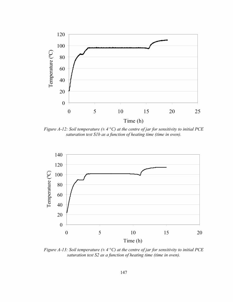
0

20

40

60

80

100

120

0 5 10 15 20 25

Time (h)

Tem

pera

ture

(ºC

)


saturation test S1b as a function of heating time (time in oven).

0

20

40

60

80

100

120

140

0 5 10 15 20Time (h)

Tem

pera

ture

(ºC)

Figure A-13: Soil temperature (± 4 °C) at the centre of jar for sensitivity to initial PCE saturation test S2 as a function of heating time (time in oven).

147

0

20

40

60

80

100

120

140

0 5 10 15 20

Time (h)

Tem

pera

ture

(ºC

)


saturation test S3 as a function of heating time (time in oven).

0

20

40

60

80

100

120

0 5 10 15 20

Time (h)

Tem

pera

ture

(ºC

)


tion test S4 as a function of heating time (time in osatura ven).

148

0

20

40

60

80

100

120

0 5 10 15 20 25 30Time (h)

Tem

pera

ture

(ºC

)

Figure A-16: Soil temperature (± 4 °C) at the centre of jar for sensitivity to grain size test

G1 as a function of heating time (time in oven).

0

20

40

60

80

100

120

0 5 10 15 20 25 30Time (h)

Tem

pera

ture

(ºC)


G2a as a function of heating time (time in oven).

149

0

20

40

60

80

100

120

0 5 10 15 20 25

Tem

pera

ture

(ºC)

Time (h)

Soil temperature (± 4 °C) at the centre of jar for sensitivity to grFigure A-18: ain size test G2b as a function of heating time (time in oven).

0

20

40

60

80

100

120

0 5 10 15 20 25Time (h)

Tem

pera

ture

(ºC)


G3 as a function of heating time (time in oven).

150

0

20

40

60

80

100

120

0 5 10 15 20 25Time (h)

Tem

pera

ture

(ºC)

Figure A-20: Soil temperature (± 4 °C) at the centre of jar for sensitivity to temperature

at sampling test C1 as a function of heating time (time in oven).

0

20

40

60

80

100

120

140

0 5 10 15 20 25Time (h)

Tem

pera

ture

(ºC)



151

0

20

40

60

80

100

120

140

0 5 10 15 20 25Time (h)

Tem

pera

ture

(ºC

)



0

20

40

60

80

100

120

0 5 10 15 20Time (h)

Tem

pera

ture

(ºC)

3: Soil temperature (± 4 °C) at the centre of jar for sensitivity to teFigure A-2 mperature at sampling test C4 as a function of heating time (time in oven).

152

0

20

40

60

80

100

120

0 5 10 15 20 25 30Time (h)

Tem

pera

ture

(ºC)


at sampling test C5a as a function of heating time (time in oven).

0

20

40

60

80

100

120

0 5 10 15 20Time (h)

Tem

pera

ture

(ºC

)

Figure A-25: Soil temperature (± 4 °C) at the centre of jar for sensitivity to tem erature

at sampling test C5b as a function of heating time (time in oven). p

153

154

A.8 Selected Laboratory Photographs

F igure A-26: Soil core segments in outer casing upon receipt in laboratory.

in PVC Figure A-27: Soil core segment #2 tubing with outer casing removed.

r filled with saturated soil aggregate andFigure A-28: Ja PCE-DNAPL.

Figure A-29: Filled open jars placed in oven for heating with thermocouple probes in

centre.

155

156

Figure A-30: Jar cap with thermocouple probe through centre for temperature

measurement during cooling in ice bath.

Figure A-31: Soil filled jar in ice bath for cooling with thermocouple probe for

temperature measurement.

Figure A-32: Soil sampling with Terra Core Sampler after cooling.

Figure A-33: 5 g soil sample after methanol extraction with clear layer of methanol

above soil for injection into purge-and-trap.

157

158

.9 Literature Cited

Engineering Properties of Soils and their Measurement, 4/e. McGraw-Hill, NY.

A

Bowles, J.E., 1992.

159

ANALYTICAL METHOD

Appendix B

160

-846: Method

pounds by Gas Chromatography/Mass Spectrometry

Series mass selective detector (MS) were used in the analysis. The GC employed a

and Mitra, 1998). In gas chromatography the mobile phase is a gas, usually helium, and

the column it is passed to a detector and a connected computer converts the detector

is displayed as a chromatogram, a plot of

e as a series of peaks which can be integrated automatically.

eak on the chromatograph is associated with the quantity of each

B.1 Methodology

The analytical methodology adopted in this study was based on USEPA SW

8260B - Volatile Organic Com

(USEPA, 1996) and, Method 5035A - Closed-System Purge-and-Trap and Extraction for

Volatile Organics in Soil and Waste Samples (USEPA, 2002). Analysis was performed at

Queen’s University’s Analytical Services Unit (ASU). Purge-and-trap (P&T) with gas

chromatography-mass spectrometry (GC/MS) was used to determine the concentration of

PCE in the soil samples. A Hewlett Packard 5890 Series II Plus gas chromatograph (GC)

with attached Hewlett Packard purge and trap concentrator and Hewlett Packard 5972

VOCOL column (60 m x 0.32 mm x 1.8 µm) manufactured by Supelco/Sigma-Aldrich

The basis of chromatography is the partitioning of a compound between a stationary and a

mobile phase. The mobile phase passes over or through the stationary phase (Kebbekus

the stationary phase is either a solid or a liquid and is contained in a column.

Compounds are separated based on their volatility and their affinity for each phase; a

compound with a higher affinity for the mobile phase will move through the system faster

than a compound with a higher affinity for the stationary phase. As the effluent leaves

signal to digital output. This digital output

detector signal versus tim

The area of each p

161

peak along the x-axis (time) is used to help identify

l

contam

it was found that the concentration was below the detection limit, the sample analysis was

repeated with a larger vo

compound, and, the location of the

the compound if more than one is present (Kebbekus and Mitra, 1998).

Soil samples which had been previously immersed in 5 ml of methanol and stored at 4 ºC

were shaken aggressively for 3 minutes. With a 5 ml gas tight syringe, aliquots of the

methanol extract was taken up along with enough organic free deionized water to form a

volume of 5 m . The volumes of methanol extract and deionized water taken up were

dependent on the expected concentration of PCE in the soil sample. If the approximate

concentration of the samples was unknown, only a small volume of extract was taken up

in order to avoid a high concentration of PCE entering and inating the system. If

lume of extract. Before injection into the P&T, the contents of

the syringe was then spiked with surrogates fluorobenzene and deuterated 1, 4-

dichlorobenzene by direct injection into the 5 ml gas tight syringe. The sample was then

immediately injected into the P&T unit. The sample was purged with zero-grade helium

for 11 minutes after which the trapped material was desorbed from the VOCARB trap by

heating and back flushing with helium for 4 minutes. The desorbed components were

then passed into the GC where the oven temperature was set to 65 ºC for 1 minute and

then was ramped to a maximum of 200 ºC at a rate of 10 ºC/minute. Each run took 24.5

minutes from injection into the purge and trap to completion of the analysis.

162

B.2 Calibration and Standards

In order to determine the linearity of the system, a calibration curve was established using

three standard solutions that covered the range of concentration expected in the

experimental samples. The calibration curve for the 5 to 428 ppb range is presented in

Figure B-1. The calibration curve showed that the detector response was linear over the

range of concentrations analyzed, with a correlation coefficient, R, and a coefficient of

determination, R2, of 1.00. As a result, it was not necessary to establish a new

chromatograph calibration curve before every day of analysis, but only to run a single

standard each day. The peak area of the daily standard Astnd was used as a factor for

calculating the concentration of the experimental samples Cex. The formula used was:

stnd

exstndex A

ACC ×= (B.1)

where C and A were the concentration of the standard solution and peak area of the

ental sample. The standard solution was prepared from a 200 ppm PCE in

facturer.

stnd ex

experim

methanol solution, purchased from AccuStandard, Inc. with a purity of 99.6 %. 100 µl of

this standard solution was diluted in 10 ml of water to for a 20 ppm standard solution. For

most analyses the concentration of the daily standard Cstnd was 40 ppb which was made by

injecting 10 µl aliquots of the 20 ppm standard solution into 5 ml of organic free

deionized water and placing the mixture on the P&T to form a 40 ppb solution within the

machine. The 20 ppm standard solution was verified for accuracy at a frequency of

approximately 10 % by comparing with a second standard purchased from a different

manu

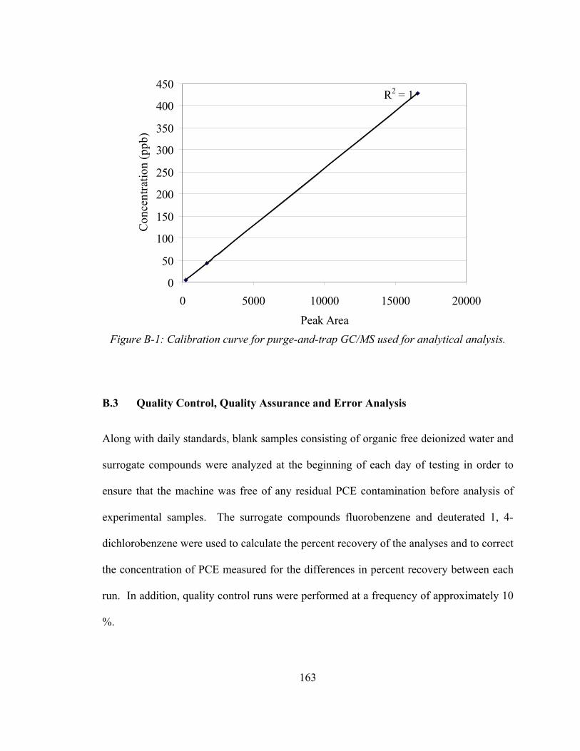
R2 = 1

50

200

250

300

350

400

Cen

tatio

n (p

pb)

0

100

150

450

0Peak Area

onc

r

B.3 Quality Control, Quality Assurance and Error Analysis

long with daily standards, blank samples consisting of organic free deionized water and

ntamination before analysis of

experimental samples. The surrogate compounds fluorobenzene and deuterated 1, 4-

dichlorobenzene were used to calculate the percent recovery of the analyses and to correct

n. In addition, quality control runs were performed at a frequency of approximately 10

0 5000 1 000 15000 20000

Figure B-1: Calibration curve for purge-and-trap GC/MS used for analytical analysis.

A

surrogate compounds were analyzed at the beginning of each day of testing in order to

ensure that the machine was free of any residual PCE co

the concentration of PCE measured for the differences in percent recovery between each

ru

%.

163

ndom or

systemati as such, should

he amount of random error present in an experimental

B.3.1 Statistical Theory

Numerical results obtained through experimentation are always accompanied by some

level of error or uncertainty (Kebbekus and Mitra, 1998). Error can be either ra

c. Random error is unsystematic and uncontrollable and

congregate around the true value. T

data set is the precision of the results. Systematic error biases the measured values either

above or below the true value. The accuracy of a data set is the difference between the

sample mean and the true value.

The arithmetic or sample mean of a data set ( x ) characterizes the central tendency in the

data. It denotes the average of all individual observations (xi) in the data set. If a sample

has n number of observations the samples mean is found by (Montgomery et al., 2004):

n

The var

sample

The squ

relative

(B.2)

n

xx i

∑ i== 1

iability or dispersion of the measurements in the data set is described by the

standard deviation, sd, (Montgomery et al., 2004):

n

164

(B.3)

e sample standard deviation is known as the sample variance (sd2). The

e

are of th

( )

standard deviation or coefficient of variation (CV) is often used to normalize th

1−n1

−=∑=

xxs i

i

d

2

standard deviation. It allows for comparison of the degree in variation between data sets

ond to no variation within the

ple, with increasing degrees of varia

When an experimental result e is calculated using multiple measured values, each with its

own uncertainty, the propagation of each uncertainty to the final result is calculated using

a number of provisional rules. If two measured quantities x, y have uncertainties δx and

δy, and an experimental result i m or the difference of the two

measured quan (Ta

δe = δx+ δy (B.5)

If the product or quotien he measured quantities x, e used to calculated the

experimental result, the uncertainty

that have drastically different means. The CV is defined as the standard deviation divided

by the mean and is often expressed at a percentage (Kebbekus and Mitra, 1998):

(B.4)

The standard deviation and CV are commonly used to measure the random error

(precision) of a measurement. A CV of 0 % would corresp

100×⎟⎠⎞

⎝⎛

xsd⎜=CV

sam tion resulting in larger values of CV.

B.3.2 Propagation of Error

s equal to either the su

tities, the uncertainty in δe is ylor, 1997):

t of t y ar

δe is (Taylor, 1997):

yxe δδδ

If an ex

uncertai

(Taylor,

(B.6) yxe

+=

perimental result is calculated by multiplying a measured value with a known

nty δx with a constant value B, the uncertainty of the experimental result is

1997):

165

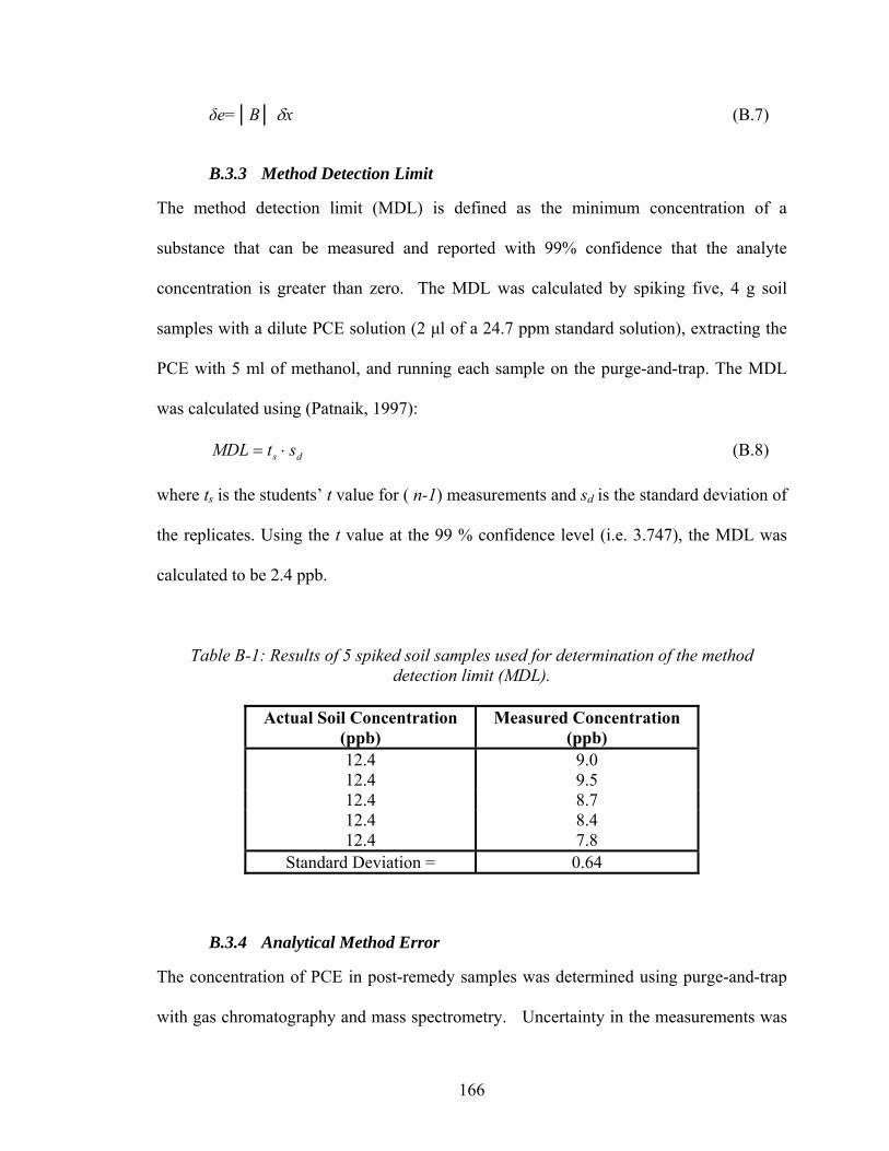
δe=│B│ δx (B.7)

The method detection limit (MDL) is defined as the minimum concentration of a

substance that can be measured and reported with 99% confidence that the analyte

concentration is greater than zero.

B.3.3 Method Detection Limit

The MDL was calculated by spiking five, 4 g soil

ples with a dilute PCE solution (2 µl of a 24.7 ppm standard solution), extracting the

(B.8)

where t is the students’ t value for ( n-1) measurements and s is the standard deviation of

the replicates. Using the t value at the 99 % confidence level (i.e. 3.747), the MDL was

calculated to be 2.4 ppb.

Table B-1: Results of 5 spiked soil samples used for determination of the method detection limit (MDL).

(ppb) (ppb)

sam

PCE with 5 ml of methanol, and running each sample on the purge-and-trap. The MDL

was calculated using (Patnaik, 1997):

s d

ds stMDL ⋅=

Actual Soil Concentration Measured Concentration

12.4 9.0 12.4 9.5 12.4 8.7 12.4 8.4 12.4 7.8

Standard Deviation = 0.64

B.3.4 Analytical Method

he concentration of PCE in post-remedy samples was determined using purge-and-trap

with gas chromatography and mass spectrometry. Uncertainty in the measurements was

Error

T

166

a result of small inaccuracies in prepared calibration standards, possible atmospheric

losses of contaminant during samples preparation, error in measuring peak areas, and

incomplete extraction of the contaminant from the soil matrix. These errors were

minimized by running quality assurance tests at a frequency of 10 %, running a

supplemental standard at a frequency to 10 % to ensure that the concentration of the

standard solution had not changed, and by limiting the exposure time of samples to the

atmosphere.

The analytical method error was determined by calculating the accuracy and precision. A

set of five 4.00 g soil samples were spiked with 100 µl of a 21.5 ppm PCE-methanol

olution to form soil concentrations of 537.5 ppb. The samples were then analyzed on the

purge- pb to

568.9 le B-2 ffici ation ( as foun 6.9

%. The systematic error (accuracy) of d was o be -2.6% using

(Kebbekus and Mitra, 1998):

ean – lue)/ true value x 100 (B.9)

Table B-2: Results of 5 spiked soil samples used for calculation of accuracy and precision of analytical method.

Name of Sample Theoretical Soil

Concentration (ppb) Measured Soil

atio

s

and-trap and GC/MS. Measured PCE soil concentrations varied from 475.3 p

ppb (see Tab ). The coe ent of vari

the metho

precision) w

calculated t

d to be

Accuracy = (m true va

Concentr n (ppb) PCE 126 (spiked soil #1) 537.5 5.3 47PCE 127 (spiked soil #2) 537.5 506.9 PCE 128 (spiked soil #3) 537.5 568.9 PCE 129 (spiked soil #4) 537.5 548.1 PCE 130 (spiked soil #5) 537.5 518.2

Mean = 523.5 Standard Deviation = 36.4

167

The measurement error associated with the balance used to measure the mass of soil in

each sample, the syringe used to measure the volume of methanol added for extraction,

and the syringes used to measure the amount of extract and water injected into the purge

od error calculated above. In order to determine the

he analytical method error, the standard practice of

raduation of each measurement as the uncertainty is

llowe es of each measurement are converted into a percentage error

nd the combined uncertainty calculated using (B.5). If the units of each measurement

ere consistent, the error would not have been converted to a percentage and (B.6) would

be used. An example of the measurement error calculation is shown in Table B-3.

Table B-3: Example calculation for measurement error in analytical method

Measurement Theoretical Measurement

Minimum Graduation of

Measuring Device

Error = ½ of Minimum

Graduation

Percent Error

and trap is accounted for in meth

measurement error independent of t

using half of the minimum g

fo d. The uncertainti

a

w

Mass of Soil in Sample 5.25 g 0.01 g ∀ 0.005 g 0.095 %

Volume of Methanol Added to Soil

5.0 ml 0.1 ml ∀ 0.05 ml 1 %

Volume of Methanol Extract Taken Up

10.0 µl 0.1 µl ∀ 0.05 µl 0.5 %

Volume of Water and Extract Injected in

Purge-and-Trap

5.0 ml 0.1 ml ∀ 0.05 ml 1 %

Sum of Measurement Error =

± 2.595 %

168

Although the method error represented by the calculated precision also includes error

he e d to be within 15 % of the method

once iked:

associated with spiking each of the 5 soil samples with 100 µl of PCE-methanol solution,

rror associated with this measurement was fount

detection limit and therefore is considered negligible. This error was found by

multiplying half of the minimum graduation of the 100 µl syringe (0.5 µl) by the

ntration of the spiking solution, and dividing by the mass of soil spc

Error = ± 0.5 µl x 21.5 µg

ml 4.00 g

Error = ± 0.00269 ppm

(B.10)

Error = ± 2.7 ppb

169

B.4 Literature Cited

Kebbekus, B.B., and Mitra, S., 1998. Environmental Chemical Analysis. Blackie

Academic & Professional, London, New York. Montgomery, D.C., Runger, G.C., Hubele, N.F., 2004. Engineering Statistics, 3/e. John Wiley & Sons, Inc., NY. Patnaik, P., 1997. Handbook of Environmental Analysis: Chemical Pollutants in Air,

Water, Soil, and Solid Wastes. CRC Press, Inc., Boca Raton, FL. Taylor, J.R., 1997. An Introduction to Error Analysis: The Study of Uncertainties in

Physical Measurements, 2/e. University Science Books, Sausalito, CA. USEPA, 1996. Method 8260B – Volatile Organic Compounds by Gas

Chromatography/Mass Spectrometry (GC/MS). EPA Test Methods, SW-846. [Online] http://www.epa.gov/epaoswer/hazwaste/test/pdfs/8260b.pdf

USEPA, 2002. Method 5035A - Closed-System Purge-and-Trap and Extraction for

Volatile Organics in Soil and Waste Samples. EPA Test Methods, SW-846. [Online] http://www.epa.gov/e test/pdfs/5035a_r1.pdfpaoswer/hazwaste/

170

171

Appendix C

MANN-KENDALL TREND TEST

C.1 Methodolo y

The non-parametric Mann-Kendall trend test is often used to analyze values of a series to

determine if an increasing or decreasing trend exists. The results of the sensitivity to

temperature at sampling tests (C1 – C5) showed no trend upon visual inspection. In order

to confirm this observation a Mann-Kendall trend test was performed. The null

hypothesis (H0) to be tested was that no trend existed. Since the heating tests were done in

triplicate, a modified version of the trend test was used in order to account for multiple

soil concentrations m ured at each temperature. The method used was based upon the

procedure outlined in EPA QA/G-9S (USEPA, 2006).

A table was constructed with a number of columns and rows equal to the number of soil

samples analyzed in the sensitivity to temperature at sampling tests (see Table C-1). The

results of the PCE soil concentration analysis were placed along the top and the left side

of the table. Every PCE soil concentration value on the vertical axis was compared with

every PCE soil concentration on the horizontal axis and a p was placed in the

corresponding box if the horizontal value was larger and an m was placed when the

vertical value was higher. Samples on the vertical axis were not compared with samples

taken at the sam am ling temperature on the horizontal axis; as a result a 0 was placed

in the corresponding box. Once the entire table had been analyzed, the number of p’s and

the number of m’s was counted. The S statistic was calculated as the difference between

the number of pluses (p’s) and the number of minuses (m’s) (Ferguson, 1965). A large

positive value would indicate evidence of an increasing trend while a large negative value

indicates evide

g

eas

e s p

nce of a decreasing trend.

172

173

Table C-1: Mann-Kendall trend test for sensitivity to temperature at sampling data (tests C1-C5) and base case (B1).

Temp. @

Sampling (°C) 4 4 4 20 20 20 36 36 36 60 60 60 80 80 80 100 100 100 100 100 100

# of p’s

11

6

4

6

14

15

6

1

0

1

1

0

6

6

4

Total

81

S=

Temp. @Sampling

(°C)

4

4

4

20

20

20

36

36

36

60

60

60

80

80

80

100

100

100

100

100

100

PCE Soil Concentration

(ppb) 14.564 19.048 22.113 18.810 11.727 9.025 17.545 24.517 44.929 19.580 21.213 25.074 11.160 12.545 14.248 16.535 22.506 18.460 18.320 14.169 13.773 # of m’s

14.564 0 0 p m m p p p p p p m m m p p p p m m 7

19.048 0 m m m m p p p p p m m m m p m m m m 12

22.113 m m m m p p m m p m m m m p m m m m 14

18.810 0 0 m p p p p p m m m m p m m m m 9

11.727 0 p p p p p p m p p p p p p p p 1

9.025 p p p p p p p p p p p p p p p 0

17.545 0 0 p p p m m m m p p p m m 6

24.517 0 m m p m m m m m m m m m 11

44.929 m m m m m m m m m m m m 12

19.580 0 0 m m m m p m m m m 8

21.213 0 m m m m p m m m m 8

25.074 m m m m m m m m m 9

11.160 0 0 p p p p p p 0

12.545 0 p p p p p p 0

14.248 p p p p m m 2

16.535 0 0 0 0 0

22.506 0 0 0 0 Total

18.460 0 0 0 99

18.320 0 0

14.169 0

13.773

81-99 = -18

C.2 Results

From the results of the sensitivity to temperature at sampling tests, the S statistic was

computed to be -18. The variance of the S statistic ( ) was then calculated using an

equation which accounts for the multiple samples taken at each temperature (Ferguson,

1965):

2sσ

⎥⎦

⎤⎢⎣

⎡+−−+−= ∑

m

s tttnnn )52)(1()52)(1(1812σ (C.1)

where n is the total number of samples (21 in this case), t is the number of samples at

each temperature (3 for all temperatures except 6 at 100 °C) and m is the number of

temperatures analyzes (5 in this case). From the variance calculated in Equation C.1, the

test statistic Z0 was computed using (USEPA, 2006):

20

)(

s

SsignSZσ

−=

where sign(S) is equal to 1 if S > 0, 0 if S = 0, and -1 if S < 0. The critical value (Z1-α) at

the 95 % confidence level (Z0.95) from the standard normal distribution table was 1.645.

The p-value from Z0 using the standard normal distribution tables is 0.279. Key values

calculated from the data in Table C.1 are presented in Table C.2.

174

Table C-2: Key parameters calculated in Mann-Kendall trend analysis

# of pluses (p’s) 81 # of minuses (m’s) 99 S -18 n 21 σs

2 1053.667 Z0 0.585 α 0.05 Z0.95 1.645 p-value 0.279

Since the test statistic Z0 was less than the critical value the null hypothesis could not be

rejected. This was further confirmed as the p-value was greater than the confidence level

(α).

175

C.3 Literature Cited

Ferguson, G.A., 1965. Nonparametric Trend Analysis: a Practical Guide for Research

Workers. McGill University Press, Montreal. USEPA, 2006. Data Quality Assessment: Statistical Methods for Practitioners. Office of

Environmental Information, EPA QA/G-9S. [online] http://www.epa.gov/QUALITY/qs-docs/g9s-final.pdf

176

Appendix D

MATHEMATICAL MODEL

177

D.1 Background

A finite cylinder with diameter 2R and length 2L (Figure D-1), initially at uniform

temperature T0, is subjected to instantaneous cooling to Tsur at all boundaries. The

temperature distribution inside the cylinder at any time involves a solution to the

cylindrical conductive heat equation (see Section 2.2) adapted from Incropera and DeWitt

(2002):

tTzrTcq

zTzrTk

zTzrTk

RrtzrTkR

rR p ∂∂

=+⎟⎠⎞

⎜⎝⎛

∂∂

∂∂

+⎟⎟⎠

⎞⎜⎜⎝

⎛∂

∂∂∂

+⎟⎠⎞

⎜⎝⎛

∂∂

∂∂ ),,(),,(),,(1),,(1 .

2 ρφφ

(D.1)

where R is the radius of the cylinder, (r, z) is the coordinate within the cylinder, T is the

temperature, t is time, k is the thermal conductivity, Cp is the specific heat capacity, is

the energy generation term, and ρ is the density of the material. With no temp

variation in the circumferential direction (

.q

erature

φ ), no thermal energy generation ( 0), and

no change in thermal conductivity with time, the cylindrical heat diffusion equation

becomes (Luikov, 1968):

.q =

tTzrT

zTzrT

rTzrT

RrTzrT

∂∂

=∂

∂+

∂∂

+∂

∂ ),,(1),,(),,(1),,(2

2

2

2

α (D.2)

With the initial and boundary conditions:

(D.3)

(D.4)

(D.5)

.)0,,( 0 constTzrT ==

surTtLrT =± ),,(

surTtzRT =),,(

178

179

Figure D-1: Finite Cylinder Used for Approximation of Soil Filled Jars (adapted from Luikov, 1968)

From Luikov (1968), the analytical solution to (D.2) is:

( )[ ]FoKLz

RrJAA

TTTtzrT

Lmnmn m

nmna

sur 222

1 10

0

expcos),,(µµµµ +−⎟

⎠⎞

⎜⎝⎛=

−−

=Θ ∑∑∞

=

∞

=

(D.6)

where:

)(2

1 nnn J

Aµµ

= (D.7)

( )m

mmA

µ2)1( 1+−= (D.8)

2)12( πµ −= mm (D.9)

LRK L = (D.10)

2RtFo α

=

n

nsionless tem

.

peratu

(D.11)

and where µ are the roots of the Bessel function of the first kind and zero order, Θ is the

dime perature, α is the thermal diffusivity, and Fo is the Fourier number.

Equations D 6 to D.11 were coded in MATLAB 6.1 and solved at T(r,z,t) = T(0,0,t), that

is, the tem e at the origin (centre) of the cylinder as a function of time. During the

perature at the centre of each jar was measured during the cooling

process usin ocouple probe and a data logger. By approximating each jar as a

finite cylinder and by imputing the dimensions of the jar into Equations D.6 to D.11,

solution lytical model were fit to the experimental data collected by varying

the valu inputted.

Verification

Values of m in Equations D.6 to D.9 were varied under constant conditions (i.e.

same ensions, coordinates, and thermal diffusivity) and plotted against

dime perature Θ to determine the values of m and n required for the

dime perature to converge. Graphs of dimensionless temperature vs. the

variables are shown in Figures D-2 and D-3. Values of 1000 were chosen for

both n to ensure that sufficient iterations of both summations were carried out. The

model was verified using an example problem on page 165 of Luikov (1968), in which a

finite cylinder, originally at 300 ºC is placed into melting ice. The temperature in the

r

laboratory tests, the tem

g a therm

s of the ana

e of α

D.2 Model

n and

time, cylinder dim

nsionless tem

nsionless tem

n and m

and m

180

center of the disk after 2 minutes was approximated by Luikov to be 90 °C. The model,

run under the same conditions, provided a temperature of 90.42 °C therefore it was

established that the model produced accurate results. In Figure D-4 the temperature at the

centre of the cylinder in the example problem is plotted as a function of cooling time, as

calculated by the model.

0

0.2

0.4

0.6

0.8

1

1.2

0 1000 2000 3000 4000 5000 6000n

Dim

ensio

nles

s Tem

pera

ture

(Θ)

Figure D-2: Dimensionless temperature vs. increasing values of ‘n’ as solved by analytical model. Points denote values of ‘n’ for which the model was solved for

dimensionless temperature.

181

0.931

0.932

0.933

0.934

0.935

0.936

0.937

0.938

0.939

0.94

0 1000 2000 3000 4000 5000 6000m

Dim

ensi

onle

ss T

empe

ratu

re (Θ

)

Figure D-3: Dimensionless temperature vs. increasing values of ‘m’ as solved by analytical model. Points denote values of ‘m’ for which the model was solved for

dimensionless temperature.

0

50

100

150

200

250

300

350

0 20 40 60 80 100 120Time ( s )

Tem

pera

ture

( °C

)

Figure D-4: Temperature at Disk Centre as a Function of Time for model verification, based on example from Luikov (1969), pg. 165.

182

D.3 Results of Analytical Model – Fitting to Experimental Data

0

20

40

60

80

100

120

0 20 40 60 80 100Time (minutes)

Tem

pera

ture

(ºC

)

120

Experimental Data B1α = 1.4e-7 m^2/sα = 1.5e-7 m^2/sα = 1.6e-7 m^2/sα = 1.7e-7 m^2/s

Figure D-5: Soil temperature (± 4 °C) at jar centre during cooling for base case test

(B1): experimental data and temperatures predicted by analytical model.

183

0

20

40

60

80

100

120

0 20 40 60 80 100 120Time (minutes)

Tem

pera

ture

(ºC

)Experimental Data H1α = 1.3e-7 m^2/sα = 1.6e-7 m^2/sα = 1.8e-7 m^2/sExperimental Data H2

Figure D-6: Soil temperature (± 4 °C) at jar centre during cooling for sensitivity to

heating time tests H1 and H2: experimental data and temperatures predicted by analytical model.

0

20

40

60

80

100

120

0 20 40 60 80 100 12

Time (minutes)

Tem

pera

ture

(ºC

0

)

Experimental Data H3α = 1.3e-7 m 2̂/sα = 1.5e-7 m 2̂/sα = 1.6e-7 m 2̂/sα = 1.7e-7 m 2̂/s


heating time test H3: experimental data and temperatures predicted by analytical model.

184

0

20

40

60

80

100

120

0 20 40 60 80 100 1

Time (minutes)

Tem

pera

ture

(°C

)

20

.Experimental Data H4α = 1.3e-7 m 2̂/sα = 1.4e-7 m 2̂/sα = 1.5e-7 m 2̂/sα = 1.6e-7 m 2̂/s



0

20

40

60

80

100

120

0 20 40 60 80Time (minutes)

Tem

pera

ture

(°C

)

100

.

Experimental Data H5α = 1.5e-7 m^2/sα = 1.6e-7 m^2/sα = 1.7e-7 m^2/sα = 1.8e-7 m^2/s



185

0

20

40

60

80

100

120

0 20 40 60 80 100 120

Time (minutes)

Tem

pera

ture

(°C

).

Experimental Data S1aα = 1.4e-7 m^2/sα = 1.5e-7 m^2/sα = 1.6e-7 m^2/sα = 1.7e-7 m^2/sα = 1.8e-7 m^2/s


initial PCE saturation test S1a: experimental data and temperatures predicted by analytical model.

0

20

40

60

80

100

120

140

0 20 40 60 80 100 120

Time (minutes)

Tem

pera

ture

(°C)

Experimental Data S1bα = 1.5e-7 m^2/sα = 1.6e-7 m^2/sα = 1.7e-7 m^2/sα = 1.8e-7 m^2/s

Figure D-11: Soil temperature (± 4 °C ) at jar centre during cooling for sensitivity to

initial PCE saturation test S1b: experimental data and temperatures predicted by analytical model.

186

0

20

40

60

80

100

120

140

0 20 40 60 80 100 120Time (minutes)

Tem

pera

ture

(°C

).Experimental Data S2α = 1.4e-7 m^2/sα = 1.5e-7 m^2/sα = 1.7e-7 m^2/s


initial PCE saturation test S2: experimental data and temperatures predicted by analytical model.

0

20

40

60

80

100

120

0 20 40 60 80 100 120Time (minutes)

Tem

pera

ture

(°C)

.

Experimental Data S3α = 1.4e-7 m 2̂/sα = 1.5e-7 m 2̂/sα = 1.6e-7 m 2̂/sα = 1.7e-7 m 2̂/s

Figure D-13: Soil temperature (± 4 °C) at jar centre during cooling for sensitivity to initial

PCE saturation test S3: experimental data and temperatures predicted by analytical model.

187

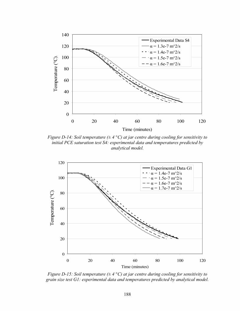
0

20

40

60

80

100

120

140

0 20 40 60 80 100 120

Time (minutes)

Tem

pera

ture

(°C

).

Experimental Data S4α = 1.3e-7 m^2/sα = 1.4e-7 m^2/sα = 1.5e-7 m^2/sα = 1.6e-7 m^2/s


initial PCE saturation test S4: experimental data and temperatures predicted by analytical model.

0

20

40

60

80

100

120

0 20 40 60 80 100 120Time (minutes)

Tem

pera

ture

(°C

).

Experimental Data G1α = 1.4e-7 m^2/sα = 1.5e-7 m^2/sα = 1.6e-7 m^2/sα = 1.7e-7 m^2/s


grain size test G1: experimental data and temperatures predicted by analytical model.

188

0

20

40

60

80

100

120

0 20 40 60 80 100 12Time (minutes)

Tem

pera

ture

(ºC

0

)

Experimental Data G2aα = 1.4e-7 m^2/sα = 1.5e-7 m^2/sα = 1.6e-7 m^2/sα = 1.7e-7 m^2/s


grain size test G2a: experimental data and temperatures predicted by analytical model.

0

20

40

60

80

100

120

0 20 40 60 80 1

Time (minutes)

Tem

pera

ture

(°C)

00

Experimental Data G2bα = 1.5e-7 m 2̂/sα = 1.6e-7 m 2̂/sα = 1.7e-7 m 2̂/sα = 1.8e-7 m 2̂/s


grain size test G2b: experimental data and temperatures predicted by analytical model.

189

0

20

40

60

80

100

120

0 20 40 60 80 100 120Time (minutes)

Tem

pera

ture

(°C

).

Experimental Data G3α = 1.5e-7 m 2̂/sα = 1.6e-7 m 2̂/sα = 1.7e-7 m 2̂/sα = 1.8e-7 m 2̂/s


grain size test G3: experimental data and temperatures predicted by analytical model.

0

20

40

60

80

100

120

0 50 100 150 200Time (minutes)

Tem

pera

ture

(°C

).

Experimental Data Test C1α = 1.3e-7 m^2/sα = 1.4e-7 m^2/sα = 1.6e-7 m^2/s

Figure D-19: Soil temperature (± 4 °C) at jar centre during cooling for sensitivity to temperature at sampling test C1: experimental data and temperatures predicted by

analytical model.

190

20

40

60

80

100

120


Tem

pera

ture

(°C

)

0

.

Experimental Data C2α = 1.4e-7 m 2̂/sα = 1.5e-7 m 2̂/sα = 1.6e-7 m 2̂/sα = 1.7e-7 m 2̂/sα = 1.8e-7 m 2̂/s


analytical model.

0

20

40

60

80

100

120

0 10 20 30 40 50 6

Time (minutes)

Tem

pera

ture

(°C)

0

Experimental Data C3α = 1.5e-7 m 2̂/sα = 1.6e-7 m 2̂/sα = 1.7e-7 m 2̂/sα = 1.8e-7 m 2̂/s


analytical model.

191

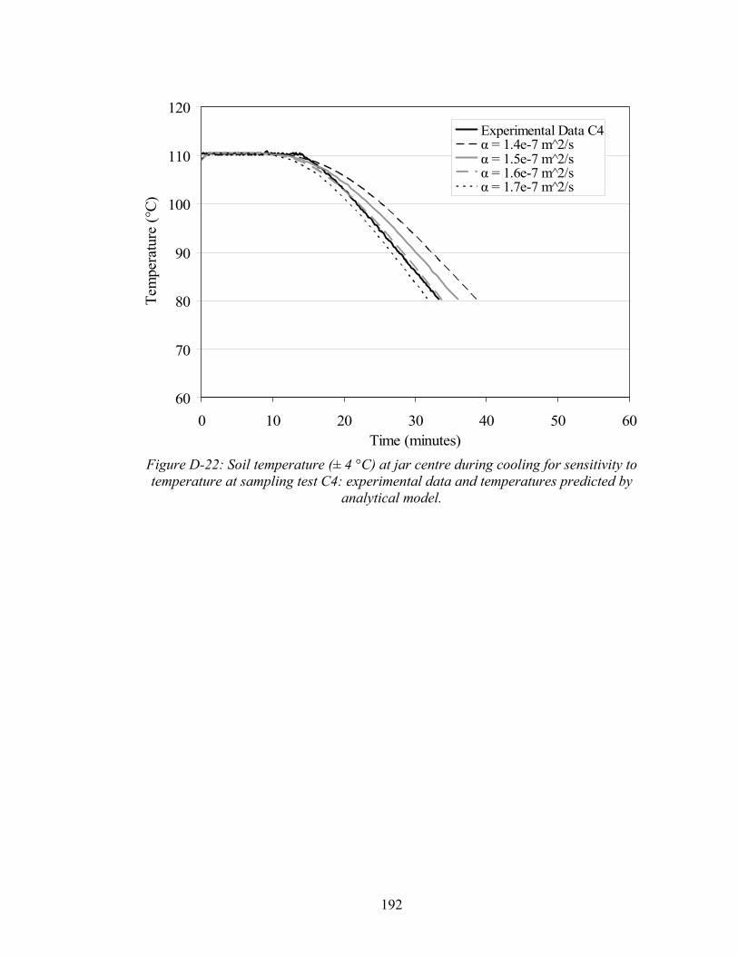
60

70

80

90

100

110

120

0 10 20 30 40 50 6Time (minutes)

Tem

pera

ture

(°C)

0

Experimental Data C4α = 1.4e-7 m 2̂/sα = 1.5e-7 m 2̂/sα = 1.6e-7 m 2̂/sα = 1.7e-7 m 2̂/s


analytical model.

192

90

95

100

105

110


Tem

pera

ture

(°C

)

0

.Experimental Data C5aα = 1.6e-7 m 2̂/sα = 1.7e-7 m 2̂/sα = 1.8e-7 m 2̂/sα = 2.0e-7 m 2̂/s

Figure D-23: Soil temperature (± 4 °C) at jar centre during cooling for sensitivity to temperature at sampling test C5a: experimental data and temperatures predicted by

analytical model.

90

95

100

105

110

115

0 5 10 15 20 25 30 35 40Time (minutes)

Tem

pera

ture

(°C)

Experimental Data C5bα = 1.5e-7 m 2̂/sα = 1.6e-7 m 2̂/sα = 1.7e-7 m 2̂/sα = 1.8e-7 m 2̂/s

Figure D-24: Soil temperature (± 4 °C) at jar centre during cooling for sensitivity to temperature at sampling test C5b: experimental data and temperatures predicted by

analytical model.

193

D.4 Example MATLAB Code

Below is the MATLAB code used for verifying the model through comparison with the

example on page 165 of Luikov (1968). In the example, the thermal diffusivity of the

material is 12.5 x 10-6 m2/s, the diameter of the cylinder is 20 cm, and the length is 12 cm.

The model predicts the temperature at the origin of the cylinder as a function of time until

2 minutes after immersion in melting ice. The file ‘jzeros’ contains a list of the roots of

the Bessel function, up to the 10, 000th root.

clear clc load('jzeros') r = 0.0; R = 0.1; z = 0.0; l = 0.06; K = R/l; a =12.5e-6; p=0; for t = (1e-3:10:120); p=p+1; for n = 1:1000; for m = 1:1000; Un = besselzeros(n); J1= besselj(1,Un); Um = ((2*m)-1)*(pi/2); An = 2/Un/J1; Am = ((-1)^(m+1))*(2/Um); J0inside = (Un)*r/R; J0 = besselj (0,J0inside); C = cos(Um*z/l); F0 = a*t/R^2; E = exp((-1)*((Un)^2+(Um^2*K^2))*(F0)); InsideSum = An*Am*J0*C*E; w(m) = InsideSum; end tot = sum(w);

194

okay(n) = tot; end final = sum(okay); Eqn(p) = final; time(p) = t; end Theta = Eqn' Time = time' plot(Time,Theta)

195

D.5 Literature Cited

Incropera, F.P., DeWitt, D.P., 2002. Fundamentals of Heat and Mass Transfer, 5/e. John

Wiley & Sons, Inc., New York. Luikov, A.V., Hartnett, J.P, (ed.), 1968. Analytical Heat Diffusion Theory. Academic

Press, New York, NY.

196

Appendix E

PROPERTIES OF PCE AS A FUNCTION OF

TEMPERATURE

197

E.1 Henry’s Constant

The Henry’s law constant is used to describe the equilibrium partitioning of a chemical

between the aqueous and gas phases (Pankow and Cherry, 1996):

w

g

CC

H = (E.1)

where H is the dimensionless Henry’s constant, Cg is the concentration in the gas phase

and Cw is the concentration in the aqueous phase. In this form of Henry’s law, the

concentrations in the gas and aqueous phases have identical units.

Using Equations 3.13 and 3.14 (Chapter 3), and values from USEPA (2001) the change in

the dimensionless Henry’s constant of PCE as a function of temperature was calculated in

Table E-1 and plotted in Figure E-1.

198

Table E-1: Data used in calculation of dimensionless Henry’s constant of PCE as a

function of temperature.

TB (K) = 394 Tc (K) = 620 TB/TC= 0.635483871

n= 0.3 ∆Hv,b (J/mol) = 34677

R (atm-m3/mol-K)= 0.00008205 R (J/mol-K) = 8.3145

HR (atm-m3/mol) = 0.0184 TR (K) = 298

Temperature (K) T (°C) T/Tc ∆Hv,T (J/mol) H (-) 293.15 20 0.472822581 38735.88953 0.590634682303.15 30 0.488951613 38376.4767 0.962399667313.15 40 0.505080645 38009.03337 1.504182942323.15 50 0.521209677 37633.10938 2.263139933333.15 60 0.53733871 37248.21307 3.288111738343.15 70 0.553467742 36853.80597 4.625883815353.15 80 0.569596774 36449.29636 6.316798298363.15 90 0.585725806 36034.03182 8.390077487373.15 100 0.601854839 35607.29037 10.85928124383.15 110 0.617983871 35168.26987 13.7183393

199

0

2

4

6

8

10

12

14

16

0 20 40 60 80 100 120

Temperature (°C)

Hen

ry's

Con

stant

[-]

Figure E-1: Dimensionless Henry’s constant for PCE as a function of temperature

between 0°C and 110 °C.

200

E.2 Vapor Pressure

The vapor pressure (Pv) of chlorinated solvents as a function of temperature (T) is usually

represented by the Antoine Equation (Reinhard and Drefahl, 1999):

CT

BAPv +−=log (E.2)

where A, B, and C are compound specific parameters. From values of A, B, and C for

PCE calculated using the Thomson method ( A=6.97683, B=1386.92, and C=217.53) the

vapor pressure of PCE as a function of temperature was calculated in Table E-2 and is

shown graphically in Figure E-2 (Reinhard and Drefahl, 1999).

Table E-2: Vapor pressure of PCE as a function of temperature calculated from the Antoine Equation.

A = 6.97683 B = 1386.92 C = 217.53

T (°C) P (mmHg) P (MPa)

37 33.71979 4.495 47 54.18397 7.224 57 84.11051 11.214 67 126.5918 16.878 77 185.3122 24.706 87 264.5655 35.272 97 369.2582 49.230 107 504.8979 67.314 117 677.5693 90.335

201

0

10

20

30

40

50

60

70

80

90

100

0 25 50 75 100 125

Temperature (°C)

Vap

or P

ress

ure

(MPa

)

Figure E-2: Vapor pressure of PCE as a function of temperature as calculated from the Antoine Equation.

202

E.3 Solubility

Knauss et al. (2000) experimentally measured the aqueous solubility of PCE as a function

of temperature. The mean solubility values measured at 1.0 MPa for each temperature are

presented in Figure E-3.

0200400600800

100012001400160018002000

0 25 50 75 100 125 150 17Temperature (°C)

Solu

bilit

y (m

g/L)

5

Figure E-3: Solubility of PCE as a function of temperature (adapted from Knauss et al., 2000)

203

E.4 Organic Carbon Partitioning Coefficient (Koc)

In Section 3.4.6, the water/organic carbon partitioning coefficient Koc

for PCE as a

function of temperature is determined by substituting values of S from Knauss et al

(2000) into (Pankow and Cherry):

(E.3)

where c and d found by Gerstl (1990) through correlation analysis were -0.346 and 1.28,

respectively. The organic carbon partitioning coefficient as a function of temperature as

calculated from Equation E.3 is displayed in Figure E-4. Since Koc describes partitioning

of PCE between the soil organic matter and water, the decreasing trend seen in Figure E-4

shows that as temperature increases, the concentration of PCE associated with the soil

organic matter decreases and the concentration in the aqueous phase increases.

dScKoc += loglog

0

50

100

150

200

250

0 25 50 75 100 125 150 175

Temperature (°C)

Koc

(ml/g

)

Figure E-4: Organic carbon partitioning coefficient for PCE as a function of

temperature.

204

205

E.5 Literature Cited

Gerstl, Z., 1990. Estimation of Organic Chemical Sorption by Soils. Journal of

Contaminant Hydrology 6, 457-375. Knauss, K.G., Dibley, M.J., Lerif, R.N., Mew, D.A., Aines, R.D., 2000. The Aqueous

Solubility of Trichloroethylene (TCE) and Tetrachloroethylene (PCE) as a Function of Temperature. Applied Geochemistry 15, 501-512

Pankow, J.F., and Cherry, J.A., 1996. Dense Chlorinated Solvents and other DNAPLs in

Groundwater: History, Behavior, and Remediation. Waterloo Press, Portland, Oregon.

Reinhard, M., and Drefahl, A., 1999. Handbook for Estimating Physiochemical

Properties of Organic Compounds. John Wiley & Sons, New York. USEPA, 2001. Fact Sheet - Correcting the Henry’s Law Constant for Soil Temperature.

EPA Online Tools for Site Assessment Calculation. [Online] http://www.epa.gov/AthensR/learn2model/part-two/onsite/doc/factsheet.pdf

LABORATORY STUDY EVALUATING THERMAL REMEDIATION OF ...

Documents

Transcript of LABORATORY STUDY EVALUATING THERMAL REMEDIATION OF ...