Laboratory Studies of the Electromagnetic Properties of Saline Ice

Year 1 Experiments, Summary

Submitted to

The Off ice of Naval Research

April, 1993

copies of this report may be obtained from:

The Goldthwait Polar Library Byrd Polar Research Center The Ohio State University

108 Scott Hall 1090 Carmack Road

Columbus, OH 43210

List of Contributors:

Kenneth C. Jezek (Editor)

Steven Ackley

Jonathan Bredow

Adrian Fung

Prasad Gogineni

Anthony Gow

Thomas Grenfell

Arion Hunt

Alan Lohanick

Jacob Longacre

Victoria Lytle

Robert Onstott

Donald Perovich

Calvin Swift

Fred Tanis

Dale Winebrenner

Ingrid ~abel

The Ohio State University

CRREL

University of Texas, Arlington

University of Texas, Arlington

University of Kansas

CRREL

University of Washington

Lawrence Berkeley Laboratory

Naval Research Laboratory

Naval Undersea Warfare Center

CRREL

Environmental Research Institute of Michigan

CRREL

University of Massachusetts

Environmental Research Institute of Michigan

University of Washington

The Ohio State University

List of Contributors

Table of Contents

Executive Summary

I. Introduction

II. Measurement Strategy

Table of Contents

ill. Summary of Laboratory Activities

IV. Preliminary Findings and New Questions

V. Next Steps

VI. Inclividual Science Reports

u

Page

ii

lll

1

3

6

9

10

12

EXECUTIVE SUMMARY

This report describes laboratory experiments conducted in early 1993 as part of the Sea Ice

Electromagnetics Initiative of the Office of Naval Research. It is a follow-on document to

the plan entitled Laboratory Studies of the Electromagnetic Properties of Saline Ice which

established objectives and scheduling for the 1993 effort. The plan called for three

measurement scenarios for 1993. These were: 1) collecting data on the microwave and

optical properties of an undeformed ice sheet grown from the melt; 2) resolving the

contributions of volume and surface scattering from an undisturbed and artificially

roughened ice sheet; 3) studying the effects on microwave signatures of brine wicking on a

snow covered ice sheet. Additional research included detailed laboratory studies of

electrical properties of cores sent to several institutions around the country. A high priority

of all the research efforts was to tightly integrate measurements of electrical properties with

ice physical properties such as salinity, structure, brine pocket shape, etc. Other critical

aspects of this phase of the project were to provide the modelling community with an

opportunity to view the methods used to collect data, to provide preliminary results to all

members of the project in order to stimulate interaction between the modelers and the

experimentalists as the experiment proceeded, and finally to provide well calibrated data for

model validation.

Experiments were conducted from January through April at the Cold Regions Research and

111

Engineering Laboratory in Hanover, New Hampshire. Extensive use was made of the new

outdoor Geophysical Research Facility as well as the indoor saline tank and refrigerated

laboratories at CRREL. All three of the planned measurement scenarios were executed in

both the indoor saline tank and in the Geophysical Research Facility. Additional, selected

research was completed in the outdoor facility known as the lower pond. Highlights

included the observation that a small amount of snow (less than 1 cm thickness) appreciably

changes the scattering response. Brine expulsion events were observed that may provide a

basis for developing methods for detecting new thin (1to2 cm) thick ice. Fully polarimetric

passive microwave experiments were conducted along with measurements with an L-band

radiometer. Continuous monitoring of the bulk dielectric constant (lOGHz) was achieved.

Laser beam spreading and transmission experiments were also conducted for the first time.

Extensive measurements of surface and near surface properties including roughness (using

a new photographic technique) and salinity were completed. Based on these observations,

several questions have been raised about the physical properties of new sea ice. These are:

1) how is brine passed from the columnar zone of ice through the transition and frazil layers

to the surface; 2) what is the distribution of brine in the transition and frazil layer; 3) what

is the dielectric roughness of the ice surface during a brine expulsion event and what is

dielectric roughness of the brine soaked snow?

IV

I. Introduction

Laboratory experiments to investigate the electromagnetic properties of sea ice were

conducted at the U.S. Army Cold Regions Research and Engineering Laboratory from

January to April 1993. Additional laboratory and theoretical studies as weU as the analyses

of data collected at CRREL are now being conducted by over 30 investigators from around

the country. The research is being coordinated under a plan entitled Laboratory Studies of

the Electromagnetic Properties of Saline Ice which was prepared subsequent to an

investig~tors meeting hosted at CRREL in September 1992. The plan was formulated as

part of the Sea Ice Electromagnetics Accelerated Research Initiative sponsored by the

Office of Na val Research. The ARI has the following goals:

* to understand the mechanisms and processes that link the morphological/physical and

the electromagnetic properties of sea ice,

* to further develop and verify predictive models for the interaction of visible, infrared

and microwave radiation with sea ice,

* to develop and verify selected techniques in the mathematical theory of inverse

scattering that are applicable to problems arising in the interaction of EM radiation

with sea ice.

1

Based on those goals and experience gained from previous laboratory, field and theoretical

research, three primary objectives were identified for experiments to be conducted at

CRREL in 1993. These were:

* measure the microwave, optical and physical properties of an undeformed, saline

ice sheet grown from the melt for subsequent use by the forward and inverse

modelers;

* determine conditions under which volume scatter or surface scatter dominates

electromagnetic signatures;

* determine the role of snow cover on electromagnetic signatures.

In addition, the experiment campaign was to be conducted under two guiding principles:

* provide preliminary results to theoreticians and other experimentalists during the

course of the experiment (foster real-time interaction amongst the various groups

and tightly integrate the modelling activity throughout the program)

* r~view all results, both theoretical and experimental, in the context of the measured

physical properties of the ice.

2

II. Measurement Strategy

Planned measurements as well as associated investigators are listed in tables 1, 2 and 3 in

the 1993 experiment plan. Prior to beginning the experiments, several additional ideas for

focusing the project were implemented. These included the establishment of criteria for

determining whether sufficient data had been obtained for successfully addressing the three

experimental objectives. The criteria developed by the team were as follows.

Undeformed Ice Experiment:

• Ice thickness > 20 cm;

* Bulk salinity < 10 parts per thousand;

• Passive microwave polarization ratios transition from new ice to first year ice values;

* Surface salinities less than 10 ppt and radar reflection coefficients reduced by at least

5 dB from skim values;

• Interference fringes in radar normal incidence data damped to <0.5 dB (relative

change).

Surface Roughness Experiment:

* At least 3 roughness scales applied to the ice sheet (0.05, 0.2 and 0.4 cm rms);

* Surface roughness data collected with comb guages, destructive sampling and

photographic techniques. On site analysis to show that:

- nns heights to within 50% of desired values;

3

- height distributions are stationary;

- Correlation functions can be fit with either Guassian, exponential or polynomial

shaped function with 95% confidence in a least squares sense;

- Surface property statistics are stationary across the ice sheet;

- Bottom roughness is characterized;

- Volume distribution of salinity and bubbles characterized.

Physical Property Sampling Intervals:

• Bulk salinity measured every 20 minutes for first centimeter of growth; every .5 cm

thereafter;

* ~urface salinity to be measured at same interval as above;

• Temperature profiles measured every 10 minutes;

• Ice surface temperature measured every 20 minutes for first centimeter of growth and

every .5 cm afterward;

• Surface roughness measured at the same interval as above.

Original planning called for snow to be applied to the ice sheet subsequent to the first two

experiments. Snow experiments were envisioned to end once the ice sheet began to melt

in the spring. These criteria formed a useful framework and were generally followed. Of

course, problems and opportunities that arose during the experiment drove changes to the

. strategy.

4

A major impact on the experiment design was the completion of the Geophysical Research

Facility. A key advantage of the new Geophysical Research Facility is simply the overall

size. The length and width of the area available for growing ice were sufficient to partition

the area into different sectors (figure 1) which were identified for smooth ice, rough ice and

snow covered ice experiments. By doing so, all investigators were guaranteed access to

control and modified surfaces.

Roof and Refrigeration

<1> 0

..c ..... 0 0 E (/)

Rough Ice

Smooth Ice

North

Figure 1

5

III. Summary of Laboratory Activities

The experiment team began arriving in Hanover, New Hampshire on January 4. Through

an extraordinary effort on the part of CRREL, the saline filled, concrete lined pool of the

Geophysical Research Facility was in place. The gantry, catwalk, and roof were all

operational in short order. The roof refrigeration units were operating by mid-January. The

indoor saline tank was also ready for use as was the lower pond. Selected experiments on

the lower pond were begun in December.

The indoor tank was used extensively in the early phase of the experiment. This occurred

partly because the activity of mounting equipment in preparation for the outdoor

experiments limited access to the gantry and partly because warm weather precluded

substantial ice growth on the outdoor pond. The intention of the indoor research was first

to conduct original experiments aimed at addressing the three science objectives for 1993.

The indoor work also served to prototype experimental techniques and evaluate equipment

for latter use on the outdoor pond. This experience proved valuable in making optimal use

of the outdoor facility. Microwave radar, laser and physical property measurements were '

conducted on undeformed thin ice, roughened ice and snow covered ice grown in the tank.

The most intensive period of indoor activity occurred between January 8 through the

January 18 after which significant ice growth began on the outdoor pond.

6

Ice/slush formation proceeded intermittently on the outdoor pond until January 18. Colder

temperatures and the use of the insulated roof enabled the team to grow ice 6 cm thick

by January 21. On January 27, investigators applied a thin cover of course grained snow to

the ice in an L shaped pattern late in the afternoon on January 27. Radiometric, radar and

optical data were acquired. Next, and based on experience in the pit, a less dense layer of

crushed ice was applied to the snow covered portion of the pond. Physical property data

including salinity and surface roughness were collected until the afternoon of the following

day when warm temperatures forced covering the sheet with the refrigerated roof. One

benefit of the warmer afternoon temperatures was that the fresh ice melded to the saline

ice surface. This may help avoid some of the problems associated with airpockets

interspersed with the crushed ice. Again a complete complement of electromagnetic and

physical property measurements was carried out.

Later in the season, a new approach to studying surface roughness was also tested. This

involved growing a layer of fresh ice on top of a precisely machined rough surface with

known roughness characteristics.

On January 30, a snow squall deposited about .. 5 cm of fluffy snow over the whole ice sheet

which had reached about 10 cm thickness. The team began to immediately collect data on

the snow covered roughened and unroughened ice and found that brine wicking strongly

modified the snow cover. Detailed (1 mm) measurements of salinity in the upper 3 cm of

the ice were made to verify where the brine originated in the ice column. Surface roughness

7

and core data were also acquired.

On January 31, a heavy snow blanketed the entire ice sheet. The snow fell at air

temperatures of about 0 F and had a density of about .05 gm/ cc. Total snow thickness was

about 19-20 cm. Additional measurements were made on both the roughened and

unroughened sides of the ice sheet. Those measurements concluded the bulk of the outdoor

experiments planned for this year. Since that time, the sheet bas experienced several

additional snow accumulations. Details of the measurements carried out on the outdoor

pond, the lower pond, and on the indoor tank are discussed in the individual science reports.

Several representatives of the modelling-component of the team visited CRREL in mid- and

late January. There, they were able to experience first hand the complexities of the ice

understudy. They also observed the experimental techniques in use in order to develop a

better sense of the strengths and limitations of different approaches.

Final experiments on the outdoor pond were conducted in April. Additional analysis of core

samples collected this past winter is planned by several members of the team (see

experiment plan). Additional experiments are planned for the summer of 1993 to be

conducted in the indoor saline tank.

8

IV. Preliminary findings and New Questions

This report is intended as a review of Year-1 activities; careful analyses of data are not

expected to be completed until the summer of 1993. Still, several interesting observations

and preliminary results are worth highlighting. These include the observation that a small

amount of snow (less than 1 cm thickness) appreciably changes the scattering response.

Brine expulsion events were observed that may provide a basis for developing methods for

detecting new thin (1 to 2 cm) thick ice. Fully polarimetric passive microwave experiments

were conducted for the first time as well as measurements with an L-band radiometer.

Laser beam spreading and transmission experiments were also conducted for the first time.

Extensive measurements of surface and near surface properties including roughness (using

a new photographic technique) and salinity were completed. Because of these observations

several questions have been raised about the physical properties of new sea ice. These are:

1) bow is brine passed from the columnar zone of ice through the transition. and frazil layers

to the surface; 2) what is the distribution of brine in the transition and frazil layer; 3) what

is the dielectric roughness of the ice surface during a brine expulsion event and what is

dielectric roughness of the brine soaked snow? Obviously, the answer to these questions will

have important implications for interpreting the electromagnetic data in terms of

contrib\}tions from rough surface and volume scattering.

9

V. Next Steps

Outdoor pond work involved learning to use the new facility and involved collection of

multisensor data sets. It is fair to say that a major accomplishment for this phase of the

ARI is the completion of the outdoor pond including the basin, gantry, walkway, roof and

refrigeration in time to collect substantial amounts of data. In that process, improvements

to the pond (and the indoor pit) have been identified and plans are being made to

implement same for next year. From an implementation point of view, the key successes

of the outdoor pond were (1) the ability to easily conduct coordinated passive, active, optical

and physical properties measurements (2) to provide enough ice such that control surfaces

could be maintained throughout the experiment; (3) to successfully maintain a 7 cm thick

ice sheet through a mid January warming thus enabling the team to take advantage of cold

weather late in the month. The essential next step is to increase refrigeration to allow ice

growth to occur in order to achieve desired thicknesses in excess of 20 cm.

The long range schedule as adopted in the experiment plan (table 4) calls for calibrated

data to be submitted to a central data base by June 1993. The data base will be available

for use by all members of the team. Detailed summaries of the 1993 experimental and

theoretical research are to be provided to the overall coordinator of the project by

September 1993 who will prepare a report for discussion at the next investigators meeting

to be held in October 1993. Topics for discussion will likely include progress towards

meeting year one objectives, new questions resulting from 1993 research, strengths and

10

weaknesses of experimental and theoretical approaches an9 facilities, modifications to the

overall plan based on 1993 experiences.

11

VI. Individual Scientific Reports

12

Accomplishments pertaining to the 1992-93 CRREL experiments University of Texas at Arlington

A.K. Fung, J. Bredow

Accomplishments

For the 1992-93 CRREL experiments we developed and demonstrated a method for controlling ice lower and/or upper boundary roughness parameters - the technique is described below. We grew two thin fresh water ice sheets that were 4 feet in diameter but of different thicknesses (2 and 3 cm), each having a smooth surface and controlled randomly rough bottom interface of Gaussian roughness with rms height = 0.25 cm and correlation length = 2.5 cm. Passive (X-band) and active (Ku-band) measurements were obtained of these ice sheets above a highly conducting medium (a randomly rough surface coated with 46% silver metallic paint). To assess the effect of the thin ice layer we also performed measurements of the lower randomly rough highly conduct­ing medium without the ice layer present. From a very preliminary look at the passive measure­ments it appears that the ice layer increased the brightness temperature (as compared to the bare highly conducting surface alone) but did not greatly affect the angular and polarization behaviors of the underlying highly conducting rough surface. The active (Ku-band) data has not yet been processed. The complete results will be made available in the mid to late spring (1993) time frame.

After completing measurements of each of the ice sheets we demonstrated that the ice sheets can be removed from the underlying highly conducting rough surface (i.e., mold) completely intact. Thereafter, the ice sheets were handled in various ways, i.e., inverting them, setting them on edge and even rolling them on edge, without damage. This indicates that they can be used in an inverted. position to assess scattering from an ice sheet with randomly rough surface and planar lower boundary. Note that one set of passive (X-band) data is expected to be available for this configuration. For future experiments we anticipate that our technique can be used to generate ice surfaces with random roughness on both upper and lower interfaces, and that thin ice sheets, with knOWJ?. surface roughness, can be married to saline or desalinated ice sheets grown in the pond.

Given what we learned at CRR.EL during the 1992-93 campaign we feel that this technique offers advantages over other techniques:

. -(1) in the study of scattering from thin, smooth saline ice with known (controlled) bottom bound-ary roughness (in this case a very thin fresh water ice forms the.lower boundary); (2) in the study of scattering from saline ice (and desalinated ice) with known (controlled) surface roughness; (3) in the study of scattering from thin saline ice with known (controlled) bottom and swface roughness (in this case very thin fresh ·waterice layers form the upper and lower boundaries); and ( 4) since for measurements performed of ice in the tank, tank rotation provides for a large number of independent measurement samples to be obtained.

Description of the e~perimental setup and technique

Documents describing the generation of random surfaces with known statistical roughness param-

cters arc available from the University of Texas at Arlington Wave Scattering Research Center (under the direction of Prof. A.K Fung). Herc it is sufficient to mention that the height distribu­tion function (and associated rms height and correlation length) and correlation function can be precisely controlled via our technique. Using the generated roughness data, a surface is milled out of a high density polyurethane foam (this material is mechanically strong and yet easy to machine). The foam surface is then painted with a highly conducting 46%-silvcr metallic paint that forms a highly reflecting surface electrically much like that of brine. Finally the surface is coated with en epoxy-based paint in order to proctect the silver and the foam from the water or brine.

In order to facilitate growth of the ice sheets a special tank was built in which to grow the ice over the randomly rough surface. This tank is connected to a stmdy swivel base that allows us to easily collect a large number of independent samples, where measurements of the ice in the tank are per­formed.

Before forming ice the rough surface is inserted into the tank with rough surface pointing up and fasteners are placed at the edges of the tank to keep the surface submerged. Then water is poured over the rough surface until the desired depth (thickness) is obtained. Then cooling is done. With the tank we found that a 4-feet diameter ice sheet up to 3-cm thickness could be obtained over­night (12 hours) provided we started with cooled water (i.e., water cooled in a cold room to near freezing) and that the temperature remained no higher than the 10° to 15° F range during freezing. Once the ice has frozen it can be removed from the mold by elevating the temperature of the mold and ice to near melting (such as indoors) while applying gentle pressure at one edge of the ice sheet. · ·

Limitations

The most significant limitation of our technique using the 4-feet diameter surface is that many of the measurement instruments have a larger footprint, particularly at incidence angles substantially away from normal. This restricted our measurement sets for the 1992-93 campaign to incidence angles less than 30°. For future experiments we are proposing to use a 6-foot diameter sllrface so that additional microwave instruments can be used, and measurements up to at least 50 to 60° incidence will be possible.

Radar Backscatter Measurements From Simulated Sea Ice During

CRRELEX'93

S. P. Gogineni, R. Hosseinmostafa and L Lockhart

We participated in controlled experiments over saline ice grown in the indoor pit during

January 1993. The primary objective of these experiments was to acquire backscatter

data in conjunction with detailed physical property measurements needed for determining

sources of scatter in saline ice. Other objectives included testing various approaches to

simulate ice surface roughness.

We performed backscatter measurements using step-frequency radars operating at 5.5 and

13.5 GHz. We started radar measurements as soon as the ice started growing. We

performed further measurements as the ice grew to a thickness of about 20 cm over a

period of six days. We collected data primarily at 13.5 GHz over incidence

angles from 0 to 50 degrees with all four linear polarizations. In conjunction with radar

data collection The Ohio State University (see the report by Zabel and Jezek) and The U.

S. Army Cold Regions Research and F.ngineering laboratory made detailed

measurements of ice surface roughness and internal structure.

After ice grew to an average thickness of about 20 cm a thin layer of snow was applied to

simulate small-scale ice surface roughness. We collected data at 13.5 GHz with all four

linear polarizations over incidence angles from 0 to 50 degrees, and at 5.5 GHz with VV

and VH polarizations over incidence angles from 0 to 45 degrees.

After completing measurements on the snow-covered ice sheet we moved the radar to the

other side of the pit and made measurements on undisturbed ice surface. Crushed ice was

spread on the ice surface and fine-spray mist was applied to make the ice cubes freeze to

the ice surface to simulate ice surface roughness. We collected a complete data set at

13.5 GHz. We found that the application of fine mist left voids and did not create a

continuous ice surface. To overcome this problem a thin layer of water was applied to

make the ice surface continuous and smooth. We collected another complete backscatter

data set after applying the water.

Figure I shows results of these experiments at vertical incidence. For undisturbed ice the

variation of the back.scattered signal across the pit was very small. Both for snow­

covered and ice-cube- covered cases there was a large variation in the backscattered

signal indicating that we increased the ice surface roughness. The experiment was

successful in acquiring data for a minimum of three scales of roughness.

--- Snow-covered Ice - - -·- - - Roughened ice

-25.o--~-....._~~~-----i · Bare Ice t == 160 mm

-30.0 - . , \ ..... . "·· .. , .. · . ... •, ...

CD :s -35.0 c .... ::J ~ -40.0 .... <l> ~ -45.0 0 a..

-50.0

-55.0....--.-~.....--r--~-T'""""""T'"~~~~~........--t-o 5 10 15 20

Relative distance

Figure 1: Backscattered signal as a function of relative distance for incidence

angle= 00

Although both methods to simulate ice surface roughness were partially successful, both

techniques suffer from the following drawbacks. Application of snow created a rough

interface, but caused internal characteristics of the original ice sheet to be altered. As

soon as snow was applied brine wicked into the snow and caused a rough dielectric

interface to form. This altered the original salinity characteristics of the ice. Since the

primary objective of these experiments was to resolve the importance of surface and

volume scatter, direct comparison of snow-covered ice with bare ice surface may not

resolve the issue.

The second method of simulating ice surface roughness by spreading crushed ice on the

original ice surface left voids when mist was applied to freeze the crushed ice to the

surface. The application of water to eliminate voids and freeze ice particles to the surface

created slightly rough ice with a few patches of very smooth surface.

In summary high-quality backscatter data in conjunction with detailed surface and ice

structure observations were collected for three types of surface roughness conditions.

These experiments allowed us to investigate in detail two techniques for simulating

ice surface roughness under controlled conditions. We believe the best and only method

to resolve the issue of surface and volume scatter is through super resolution experiments.

CRRELEX'93 Participation by CRREL

Ors. Anthony J. Gow and Donald K. Perovich

As in the past, CRREL personnel supervised the fabrication of saline in sheets and monitored their temperature, sal inity, and structural characteristics in conjunction with active and passive microwave imaging. Both the new outdoor facility and the indoor refrigerated tank (pit) were utilized in this yea.r's investigations.

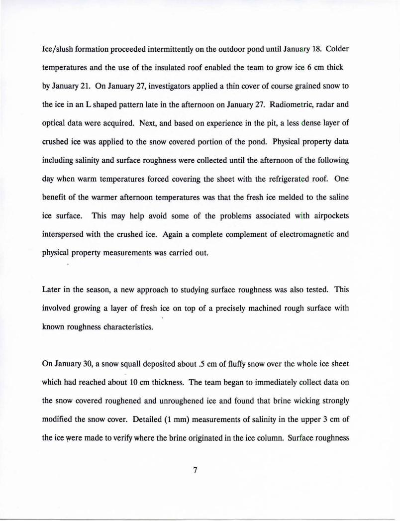
Pit Studies: These were initiated on 8 January using a salt water concentration of 30%. Temperatures in the pit were maintained at -180C throughout the experiment. Active r adar measurements were performed (1) to evaluate initial growth signatures and (2) to examine the effects of various scales of roughness on the radar scattering characteristics. Surface roughness was modified through use of snow and ice chips carefully spread on top of the ice sheet. The ice was coarse­columnar in texture throughout due to the spontaneous nucleation (without seeding) nature of the initial freezing. Ice platelet/brine inclusion structure of the crystals simulated precisely the structure observed in arctic lead ice grown under similar quiet conditions of freezing. A detailed study of surface, incremental and bulk salinities was performed throughout the entire growth history of the ice sheet. Salinity profiles for 7 cm and 15.5 cm thick ice are presented in Figure 1. Both demonstrate the c-shaped profile that typifies thin (lead) ice growth in the arctic. Additional studies in the pit included investigations of the surf ace roughness elements using bulk optical and mechanical (comb) techniques. Resules are currently being evaluated.

Pond Studies: Studies in .the new pond were confined to measurements on a single ice sheet. The pond contained water with a bulk salinity of 29-30%. at the outset of the experiment. Ice growth was initiated during the evening of 18 January. As with the pit, the pond water was allowed to nucleate spontaneously, leading to the formation of coarse-grained columnar ice. Ice thickness increased only slowly to about 6 cm by 21 January and to 8.7 cm by 30 January. Surface air, in situ ice and water column temperatures were measured continuously via a string of thermistors. Surface salinities and ice salinity profiles were monitored at regular intervals together with measurements of crystalline structure/brine pocket characteristics on samples cut from the growing ice sheet. Effects of a snow cover, including brine wicking, on microwave signatures were investigated. Surface roughness effects created by broadcasting ice chips onto the surf ace of the ice sheet were also examined . Optical and comb techniques of examining surface roughness were also applied. Salinity profiles for ice after 6.3 cm and 11.8 cm of growth are presented in Figure I. Both profiles are c-shaped. However, corresponding salinity is much

lower for the 3 February profile, reflecting the desalinating effects of periodic elevated air temperatures throughout the ice growth process.

At this time we are proceeding with the detailed thin sectioning and photographing of samples of ice from both the pit and the pond.

Indoor pit 0..--------...--~~~ -----=::;.--0

4

~

E ~ 8 ..c +-' 0. Q)

0

12

Q

0 () -•-10 Jan

cJ -0-12 Jan

/ I 1·~

0 ·~ \ "'-0 • I

0

I 0 I

0 \ 0 \ o'\ / 0

a \ 0

Outdoor pond

-•-21 Jan -0-3 Feb

4

0 CD

"'C ast ~

0 3 ..._...

12

16"--_.__..___._ __ .....___._ __ .....___.____. _______ ....._ ____ ...._ ____ ....._ ___ ____. 16

0 5 1 0 15 20 0 5 1 0 15 20

Salinity (o/oo) Salinity ( o/oo)

1993 CRREL Experiments

Thomas Grenfell Unversity of Washington

Congelation Ice Growth Experiment -- We utilized the first cold snap available to us (on 18 January) to begin this phase of the experiment with participation by passive microwave (UW), active microwave (ERIM and UMass) and optics (ERIM, NRL) investigators . Although the 35 GHz UMass scatterometer could not be set up in time for the first centimeter of ice growth, the data from that point on include a good number of independent samples; this should make this a very useful data set in addressing the surface vs. volume scattering question.

The passive microwave measurements included multipolarization measurements of TB and emissivity at frequencies of 6.7, 10, 18 .7, 37, and 90 GHz. Simultaneous measurements were made in the thermal infrared (8-14 microns) to determine ice skin temperature and infrared emissivity. This year we modified our mounting hardware to al l ow us to measure the first 3 components of the Stokes vector for all 5 microwav·e instruments. At 10 and 37 GHz we used quarter wave plates to obtain the 4th component giving us fully polarimetric passive observations at these two frequencies . The observation set included primarily angular scans from 40 to 70 deg nadir angle, sky observations for calibration and calculation of emissivity, but we also carried out spatial scans to investigate surface homogeneity. A preliminary quick look i ndicates that during the congelation phase the ice sheet was indeed homogeneous to within a few degrees K. Each day we timed our measurements to correspond with visible-infrared albedo observations carried out by D. K. Perovich. Since albedos could not be made at night or when the roof is on the pond, we have concurrent data only for a limited number of cases, but these spanned the entire growth sequence and the roughened and snow covered surfaces.

Certain benefits of the new facility became quickly apparent. We now have plenty of area to leave a control area big enough t o accommodate the set of instruments involved in the proj ect, and the ice sheet did not deform (ie. sag) a necessary condition to preserve homogeneity especially close to the edges of the pond where we did much of the characterization.

We obtained a considerable number of surface scrape samples to investigate the magnitude and variations of the salinity of t he surface brine layer . Using the temperature profile observations and our measurements at the surface we will be able to determine the behavior of the brine volume . We used our new microprofiling technique, which allowed us to shave off 1 mm layers to a depth of 5 mm, and Wensnahan's core slicer ("the slicer dicer"), which gives about 3mm resolution for cores up to 30 cm long . These measurements were continued throughout the experiment. Ingrid Zabel was very helpful and obtained several sets of observations when we were especially loaded down doing radiometry.

The roof and refrigeration components of the new facility proved invaluable during the warm spells. We were able to cover the ice , keep

it cold and hold the salt in it each time . In fact, we even growth as long as the air temperature was below about 40oF . key factor in allowing us to obtain saline ice thick enough the roughening and snow cover experiments .

got s ome This was a

t o carry out

Surface Roughness Experiment -- After the congelation sheet had reached about 8 cm we deposited a light dusting of snow on ab out 50% of the surface leaving the other 50% undisturbed. We obtained a series of 4 observational sequences as the snow bonded to the surface . The surface was then roughened further by adding crushed ice and the observations were repeated . Each observational sequence consisted of a full set of measurements over the roughened area together with another full set over the undisturbed control area. A preliminary check suggested that the roughened surface did affect the emissiv ities especially at the highest frequencies .

Snow covered surface measurements -- After the roughness expe rimen t s were completed we left off the roof and allowed 18 cm of snow to f all on the ice . Brightness temperatures were obtained at several stages of deposition when the snowfall rate was low enough to avoid clogging our antennas . Observations were continued until water seepage from under the ice infiltrated the snow pack . It is not yet clear whe ther we we r e ab l e to observe the effect which decreases PR to the value found f or pol a r FY ice, but we were able to check the cases scheduled for this year 's operation.

Passiue Microwaue Obseruations in Support of the EM/RR I

(Measurements done in Jan-Feb 93) Alan Lohanick

The field season up to now:

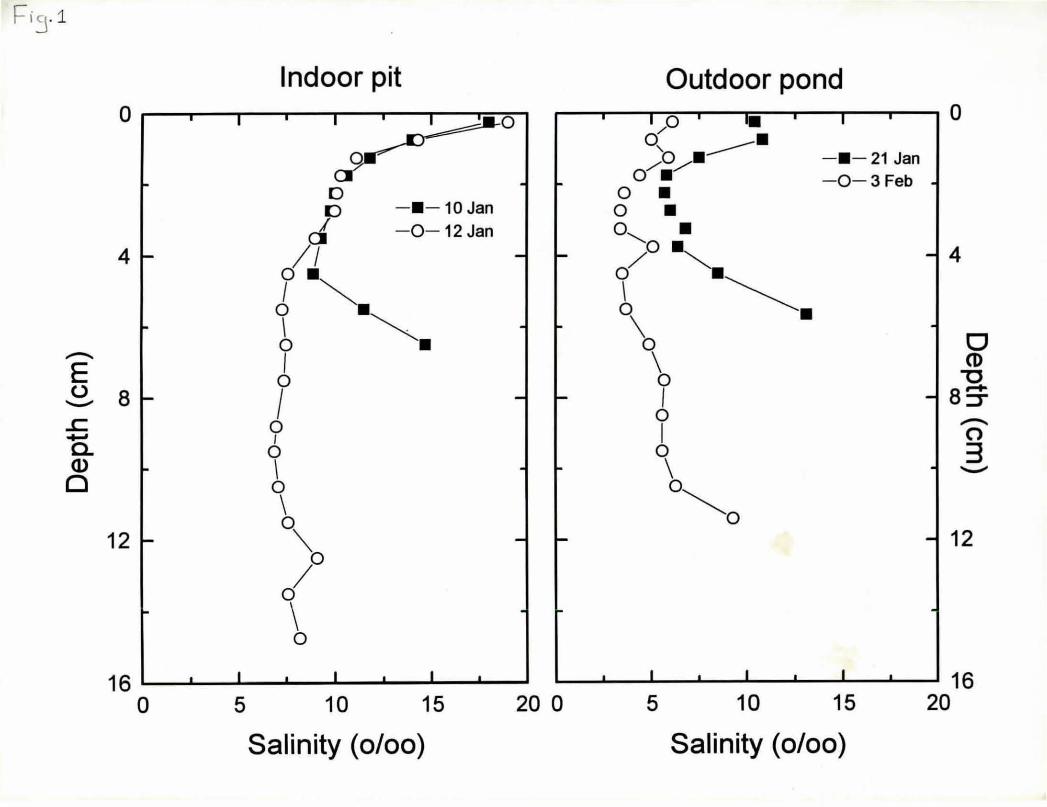
We beg1m in December with 24 ppt water in the "lower pond". The early part of the winter was mild, so ice h8:1 grown to only about 1 O cm by 1 Jan. We chose to wait for further growth, and also to prevent a snowcover unt11 the lee was over 20 cm thick. To contrast with earlier work, we wanted to hove a reosonable snow cover which would still not weigh down the ice to below freeboard ( in such a case, only the wicking ~tion and thermal conductivity of the snow serve to red1strlbute the brine). Of course, because of the mild season, the lee was somewhat desalinated and bubbly in its upper layer, and in early Jan we measured about 10-15 ppt bulk salinity in the top 1 to 2 mm of the ice. We obtained brightness temperatures of the bare ice during January. On 28/29 January, we allowed a 1 cm snow cover to fall on the ice, and took r8:1iometer data that day and on the following evening, when the snow hOO been reduced to a few mm, apparently by wind. We also obtained some microphoto;iraphs of the fa111ng and in-pl~ snow. The changes in brightness temperature due to the snow have not been calculated as yet. V. Lytle took a full core sample on 28 Jan for later determination of dielectric constant. The snow cover in effect disappeared In a few days, probably as a result of wind and the 1ncorporat1on of the snow into the top layer of ice. The ice reached 18 cm in thickness at the end of January.

On 6 Feb at the ORF, we began a series of cooperative brightness temperature measurements at I 0 and 37 GHz on the manufactured surface brought by J . Bredow of U.Texas Arlington. We looked at the bare surfa, and at fresh water, freezing water, and 1ce over the surf~. Although the surf~ was somewhat small for the beam pattern of the 1 O GHz rooiometer, we p loced reflective material around the setup, and hope to get ipxi calibrations using the open water data. John took rooar measurements later In the week on similar surf~ ( 1.e. another batch of water).

On 15 Feb we returned our Instruments to the lower pond In ant1c1pat1on of a snowfall the following day. We ro11a1 the roof off the lee surfoc:e late on 15 Feb , and about 24 hours later repl~ It over the lee, while snow was stm fa111ng. About 15 cm of snow hoo ax:umulated. Our thermistor arrey date showed that the vertical temperature grooient of the ice hOO been greetly reduced by the snow cover, as was expected bEK:SUSe of the insulating effects of the snow. We measured the oonslty of the snow as 0.09 gm/cc (or 90 kg/m3).

On 19 Feb, when the thickness of the snow hoo reduced to about 9 cm , we began brightness temperature meesurements. We also obtained snow samples for later phota;Jraphing, and measured the snow density ( 100-125 kg/m3). We obtained 2 full cores on 20 Feb for later structure char~terlzatlon and dielectric constant ootermlnatlon. Freeboard In both core holes wes slightly over I cm. Verticel temperature profiles were of course obtained during this time. The ice surfo remained "perf~tly" flat, and the crystals in the bottom layers of the snow cover were not being fncorporatoo Into the tee surf~. Bulk salinity of the lowest layer of snow was measured at about 30-35 ppt, demonstrating the wicking ~tion of the snow.

As of 1 Mar, the snow thickness WGS about 6 cm, and its li3nsity about 135 kg/m3. We intend to obtain brtghtness temperatures durtng Mar, and. ebta1RiftEJ at least one more set of cores end snow samples for a complete case history with a thinner and more dense snow cover.

Measurements of the Complex Dielectric Constant of Sea Ice at Frequencies from 26.5 to 40.0 GHz

Preliminary Report of Measurements during January and February, 1993

V.I. Lytle and S.F.Ackley

The goal of these experiments is to experimentally measure the transmission time, and the losses through a sea ice core. Using these measurements, the complex dielectric constant of the sea ice can be calculated. This is a non­destructive method which allows details of the stratigraphy of the specific sample to be measured, and later correlated to the dielectric properties of the ice .

During the first year of the CRRELEX experiment, the objectives were to calculate the dielectric constant of the sea ice grown in the various facilities at CRREL; the indoor pit, the outside lower pond, and the new outdoor sea ice facility. lOcm diameter cores (4 inch) were collected from the three different locations. Four different samples from the indoor pit were collected to allow the measurement technique to be refined, and to estimate the sample to sample variability. Cores from the outdoor facility were collected on January 30, from both ends of the pond; one core where the snow had been swept off, and one core where the snow had been allowed to accumlate. An additional two samples were collected on February 12, after the ice sheet had partially desalinated. One core was collected from the lower pond on January 24. Additional cores will be collected during the rest of the winter as the outdoor ice sheets continue to grow and desalinate.

The samples were stored at -2oc, to minimize brine drainage. However, some brine drainage occurred during the time the core was extracted and transported to the cold room for storage. To prepare the samples for the dielectric measurements, they were cut into lengths varying from 5 to 8cm. The ends of the ice core were milled plane and parallel to within .002 11 to eliminate the effects of surface scattering . The dielectric measurements were collected within one day of the milling to minimize the effects of sublimation. All the measurements reported here were collected at a temperature of -lOC. It is planned to collect additional measurments at lower temperatures, because of logistical constraints, these will be done at a later date.

A Hewlett Packard 8510 system was used to measure the time of transmission and the losses through the sample. It is configured as a step-frequency radar, and uses a single horn antenna for both transmission and reception of the signal . The system operates at a bandwidth from 26.5 to 40.0 GHz (Ka-Band). It is internally calibrated using a

series of standards, and was found to be quite stable even at these lower temperatures. The system effectively transmitts a short pulse, polarized electromagnetic wave which travels through the sample. The instrument measures the reflection from the top and bottom surf ace of the core sample, and these are then used to calculate the complex permittivity. An example of the output from a single measurement is shown in Figure 1. Each of the samples was measured with the electric field oriented in 4 different directions co0 , 45°, 9o0 , 135°). Although these samples are not expected to be anisotropic in the horizontal plane, these measurements will allow us to confirm this assumption. To obtain a better average permittivity, and to estimate experimental error, additional measurements were collected with the electric field oriented at 180°, 225°, 210° and 315°. The o0 line on the samples was arbitrarily chosen. A total of 8 different samples were measured, and the permittivity has been calculated. Additional measurements will be done at lower temperatures, and on additional cores collected as the ice continues to desalinate.

The results of these measurements, and the calculated dielectric constant are shown in Table 1. These are preliminar estimates, and the results have not been corrected for the effects of defraction. Howevr, it is expected that this correction will change the results by less than 2%. The values reported here are averages of all the measurements on a single sample. The salinity of the core samples ranged from about 6ppt to 9ppt. At the higher salinities, the losses were so great it was not possible to estimate the imaginary part of the permittivity. The milling jig will be modified to allow us to collect data on smaller core samples, and to estimate the permittivity on these high salinity samples. The real part of the relative permittivity ranged from 3.17 to 3.44. The imaginary part of the relative permittivity ranged from about 0.05 to 0.13, and correlated well with the salinity. At this time, the thin sections work has not been completed so it is not possible to directly compare the results to the specific ice morphology. However,it is possible to compare the results with salinity measurements, and with data collected using the same technique on multi-year cores collected in the field. As found in the previous study by Rennie (1991), the imaginary part of the dielectric constant largely dependent on the salinity of the sample.

Future work this year will include measurements at lower temperatures, and on samples collected later in the year as the outdoor ice sheets delsalinate.

Core Sample Location

Indoor Pit

Indoor Pit II

Lower Pond

Depth (cm)

1-7 1-7 3-9 7-14 13-19 19-25 19-25

2-8

Salinity El EH

(ppt)

9.0 3.44 -··-7.4 3.42 0.13 • 3.37 0.10 • 3.39 0.07 6.8 3.38 0.11 • 3.19 0.06 5.9 3.19 0.09

* 3.17 0.7

Table 1 *Salinity values will be measured after thin sections are completed.

** Imaginary part of the dielectric constant greater than 0.2.

Figure 1 Time domain response from ice core. The large return is from the top of the ice core, the smaller return, with the marker is from the bottom of the ice core. The transition from the waveguide to the horn antenna can be seen earlier in the signal.

S11 L I!JEAR REF - 50.0 rnUnit "$:

f.y 2 0 . 0 mun i t $ /

"' 1 3 . 2lA mU. !iii . . - ---. -1 -· I I I I

c r f'.ti ARkER l i-- -·- - -

M

I 3.91875 ;ns • I :·1. 17i4a· .n·: I : ,

i I : ·- ··- --··! '

I I

..J _ _ --r - -- - I - -·

!

i

! ' - .

~-

- -· .. ' ·-·- ·--

.l --·-I

-1 !

,_ - - --. '

i

· - - -+ I

'

j •• • • •• I

i ' I ~ t I .>- ·~- - l ···- ---L - --- --L . - --

START 0.0 s S TOP 5.0 :is

I

_J._ ·- .. -L I '

l I ! I r -· ·· r i I I 1

--l--- ·-- ·- · _J _ - - - -

- l I

' i I

- 1 i I

ELECTROMAGNETICS OF SEA ICE - Report of ONR/ ARI 1993 Activities at CRREL -

Rohen G. Onstott Environmemal Research Institute of Michigan

SUMMARY OF ACTIVITIES Included herein is a reporting of activities performed at the U.S. Army Cold

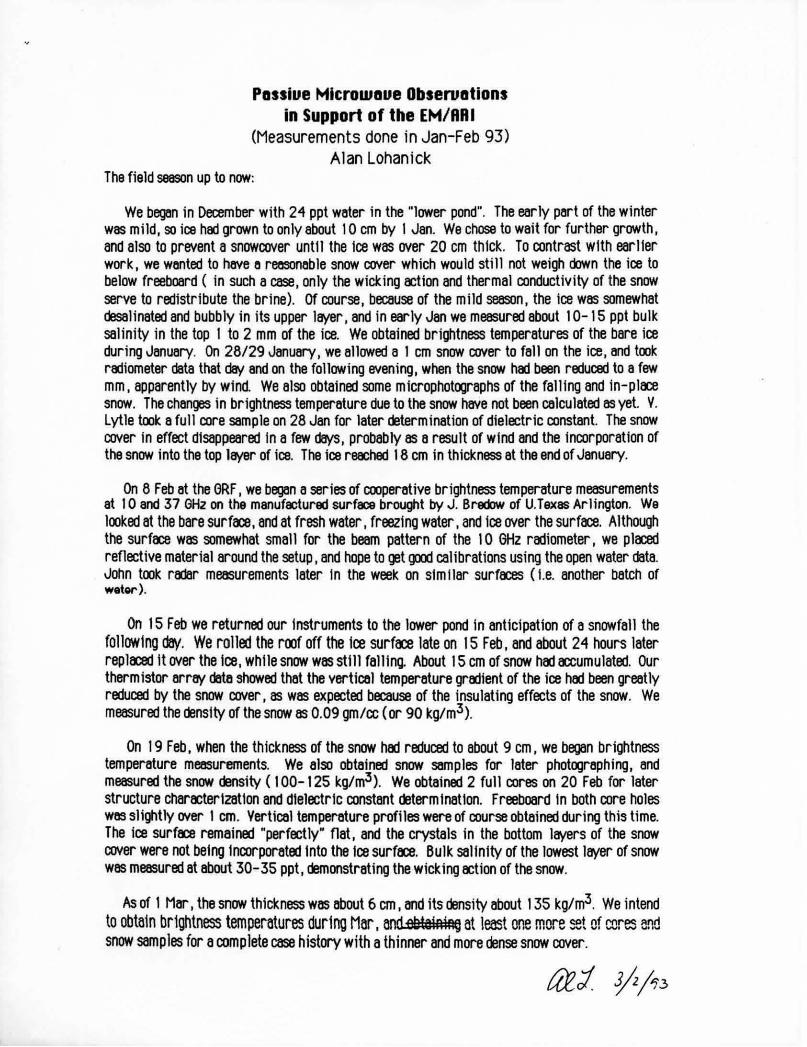
Regions Research and Engineering Laboratory in support of the Office of Naval Research Accelerated Research Initiative addressing the electromagnetics of sea ice. During January of 1993, saline ice was grown in two separate facilities, an outdoor and an indoor tank. The major experiment thrust was conducted in the outdoor facility, new for FY-93. The sea ice tank is about 7.6m x 18.3m x 2.lm (width x length x depth). Supporting facilities include a 3. 7m high moveable gantry and a lm high moveable gangway. Air conditioning and a moveable insulated roof aids in the preservation of an ice sheet when ambient temperatures approach or exceed -1.8° C. The gantry was used to support the mounting structure for the polarimetric radar antenna arrays and could be positioned easily along the length of the sea ice tank. An antenna mounting structure was developed to allow positioning along the width of the tank and to facilitate the electromechanical setting of the incidence angle of the radars (range from 0° to 135°). A summary of instruments utilized and type of measurements performed at the outdoor tank are summarized in Table 1. An abbreviated summary of sensor parameters is presented in Table 2. Investigations at the outdoor tank focused on the role surface and volume scattering play in determining the electromagnetic response of sea ice. This was accomplished through an ice growth experiment and an experiment series where the air­ice interface was perturbed, thereby enhancing the roughness of this interface without effecting internal ice sheet properties. This approach was taken to document the contribution of interior ice permi~tivity fluctuations and their ability to produce volume scatter, and the contribution produced by surface scatter. A summary of the specific observations made are presented in Table 3. Other investigations included observations of smooth and bare ice sheets at multiple air temperatures in the range from 0°C to -25°C, and the impact of a thin (4mm) and thick (19cm) layer of snow on smooth and rough ice. During the ice growth experiment, optics-and-microwave observations were made (Fred Tanis I ERIM and Don Perovich I CRREL). In addition, measurements were coordinated with passive microwave observations (Thomas Grenfell I University of Washington) to document the microwave signatures from 6 to 90 GHz.

In an indoor facility the importance of surface roughness for a thick (24cm), saline ice sheet was documented using various techniques to perturb the air-ice interface. Observation of the backscatter response assisted in evaluating the utility of various roughness perturbation approaches. The results of this work were applied to the studies conducted at the outdoor facility . A quad-pol X-band radar (X-SCAT) was used in support of this work.

The optics-microwave response (F. Tanis I ERIM) of evolving new ice was repeated indoors for a constant air temperature (about-19°C). The purpose of this work

was to obtain additional data to examine the ability of both optics and microwaves to provide information of the internal properties of a saline ice sheet. Activities conducted in the indoor tank are summarized in Table 4. In Figure 1 the microwave backscatter (30° incidence) at VV, HH and cross polariz.ations and dielectric constant (magnitude) data were obtained for ice thicknesses ranging from 5-38 mm. These data show oscillations for thin ice thickness values which may be associated with coherent effects which may arise due to the parallel interfaces (air-ice and ice-water) of a thin plate of sea ice. Effects of this type have previously been discounted. Additionally, the polarization response is most dramatic for very thin ice and is shown. Coherent effects and the polarization response will be under study and used to improve the theoretical modeling of scattering from ice layers thinner than the wavelength of the observing sensor, and in determining if and how this additional information may be exploited and related to internal ice sheet properties.

The reflectometer developed to measure dielectric constant (operating wavelength of 3cm) appears to have performed admirably and will provide a record of the magnitude of the dielectric constant measured in situ. These data will be combined with data obtained using the polarimetric radars (when operated at nadir) to produce a frequency response record of dielectric constant for the various ice forms.

Eleven surface roughness slabs were processed to obtain a statistical description of the air-ice interface for surfaces observed in both the indoor and outdoor facilities. Data were obtained to describe the change in roughness as the ice sheets evolve.

Acknowledgement There is a large cast of people from the various institutions who are supporting

this ARI not mentioned above and have made important contributions to the success of this investigation. Their efforts are greatly appreciated.

Table 1. Instruments and Methods Utilized During ONR-EM-ARIJanuary 1993 Activity [Onstott/Active-Microwave].

INSTRUMENTS and MEASUREMENTS

Fully Polarimetric Active Microwave Sensors Frequencies of operation from 0.4 to 95 GHz. Range and frequency data recording. Range resolutions in free space from 5 to 15 cm. Installation at the outdoor sea ice tank facility.

Dielectric Constant via Microwave Reflectivity Reflectometer observations at 10 GHz made continuously. Observations at 0.4 to 95 GHz made periodically. Utilized in both the outdoor and indoor facilities.

Color Video VHS recordings made during the radar observations. Camera boresighted with the polarimetric radars and view varied with

incidence angle.

Environmental and Ice Sheet Observations Surface roughness observations made using high vertical-and-horizontal

resolution method (Onstott). Tair, Tice, and Salinity (profile and surface). Color Photography

35mm obliques are time coded. macrophotography of selected features.

Table 2. Microwave Sensor Measurement Matrix During ONR-EM-ARI January 1993 Activity [Onstott/Active-Microwave].

SYSTEM FREQUENCY POLARIZATION INCIDENCE - GHz- ANGLE

POLRAD 0.4, 1.25, 2.25, Fully Polarimetric 0°- to-60° - outdoor- C.C.- 5.25, 9.38, 35 & 94 15 ° Increments

Reflectometer 10.25 -- oo - indoor a: outdoor- f ac .-

X-SCAT 9.5 Quad-Polarization 0° -to-47 .5 ° - indoor fac. - 2.5° Increments

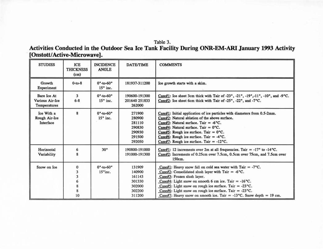
Table 3. Activities Conducted in the Outdoor Sea Ice Tank Facility During ONR-EM-ARI January 1993 Activity [Onstott/ Active-Microwave].

STUDIES ICE INCIDENCE DATE/TIME COMMENTS TIDCKNESS ANGLE

(cm)

Growth O-to-8 oo-to-600 181937-311200 Ice growth starts with a skim. Experiment t5° inc.

Bare Ice At 3 oo-to-600 t90600-t9t300 Case#l: Ice sheet 3cm thick with Tair of-23°, -2t 0, -19°,-11°, -to•, and -9°C. Various Air-Ice 6-8 15° inc. 201640 251833 Case#2: Ice sheet 6cm thick with Tair of -25°, -22°, and -7°C. Temperatures 262000

Ice With a 8 0°-to-60° 271900 Case#l: Initial application of ice particles with diameters from 0.5-2mm. Rough Air-Ice 15° inc. 280900 Case#2: Natural ablation of the above surface.

Interface 281110 ~: Natural surface. Tair = ~·c.

290830 ~:Natural surface. Tair = o•c. 290930 ~: Rough ice surface. Tair = 0°C. 291500 Case#6: Rough ice surface. Tair = -4 °C. 292050 Case#?: Rough ice surface. Tair = -l2°C.

Horizontal 6 30° 190800-191000 Case#!: 12 increments over 2m at all frequencies. Tair = -17° to -14°C. Variability 8 191000-191300 Case#2: Increments of 0.25cm over 7 .Scm, O.Scm over 75cm, and 7 .Scm over

lSOcm.

Snow on Ice 0 0°-to~0° 131909 Case#!: Heavy snow fall on cold sea water with Tair = -7°C. 3 15°inc. 140900 Case#2: Consolidated slush layer with Tair = ~·c.

3 16ll43 Case#3: Frozen slush layer. 6 301330 Case#4: Light snow on smooth 6 cm ice. Tair = -l6°C. 8 302000 Case#5: Light snow on rough ice surface. Tair = -23°C. 8 302200 Case#6: Light snow on rough ice surface. Tair = -23°C. JO 311200 Case#?: Heavy snow on smooth ice. Tair = -13°C. Snow depth = 19 cm.

Table 4. Activities Conducted in an Indoor Sea Ice Tank Facility During the ONR-EM _ARI January 1993 Activity. Air Temperatures from -17° to -19°C [Onstott/Active-Microwave].

STUDIES ICE INCIDENCE ANGLE DATEffIME COMMENTS TIIlCKNESS

(cm)

Smooth & Bare 24 0°-to-45° @ 2.5° inc. 141000 Natural undisturbed ice growth . Tice = -9.7°C. Surface roughness sample obtained.

Dielectric 24 0°-to-45° @ 2.5° inc. 141605 Case#l : Fine snow (0.25-.5 cm) used to create dielectric Roughness roughness layer. Measured immediately after application to

observe initial brine wicking into snow layer. 151027 Case#2: Surface cooled overnight allowing brine to redistribute.

Slightly Rough & 24 0°-to-48° @ 2 .5° inc. 151139 Ice surface has roughened due to ablation of th.e ice-air interface Bare due to evaporation. Surface more rough than the above. Tair =

-17"C & Tice = -11.1 •c. Surface roughness sample obtained.

Large-Scale 20 O"-to-48° @ 2.5°inc. 151653 Case#l : Small ice cylinders (5 mm diameters with about 1 cm Roughness 1 location examined lengths) were deposited on the ice surface.

2 locations examined 161002 Case#2: Cubes and surface sprayed with a light mist of fresh water to further bond roughness elements and fill air voids.

2 locations examined 170939 Case#3: Cubes and surface sprayed until saturated with fresh water to further fill air voids and reduce roughness.

Horizontal Variability 171018 Case#4: Horizontal variability examined at 12 locations at 0 ° and 12 locations examined 30°. Visual roughness variations noted. Surface roughness slabs

0° & 30• retrieved to describe these variations. New location in middle 171059 Case#5: Angle response at new location about I meter up from

of roughness area the previous set of locations. Surface is smoother at this position.

Optics-Microwave O-to-5 30° 201323-211115 Coordinated optical transmission (F.Tanis), dielectric constant and lee Growth microwave backscatter measurements conducted of growing ice at Experiment a constant air temperature of -19°C.

Observations of 8 0°-to-45°@ 2.5° inc. 221035 Case#l: Reference scene with frost flowers beginning formation. Prost Flower 30° 221152-251245 Case#2: Formation underway. Examined continuously over an

Growth extended pe riod at 30°incidence. Dielectric constant monitored.

Normalized Radar Backscatter Power (dB) I I I

~ I\) ...... ...... 0 0 0 0

0

l

x ~ j

0 "O

...... -0 0 t/) I

-~ ::J -· CL O 0

..., () 0 <D 0 ~ ..., ~ C/) $» :::J'" ()

(1) < A" $» (1) ::J I\) - Ci) <D 0 0 ..., fJ) (1) 0 fJ)

"Tl~ ......... 3 $» ::J" 3 0 =m -· >< ~"O

(1) ::::!. 3 (1) ::J -

0 N

Dielectric Constant Magnitude 0 0

UMass CRRELEX '93 Activity Summary The meeurcments we obtained thi11 year were uing a 35GHz ecatterom­

eia. Thia instrument ia bued &round an HP 8510 Newtork Ana.lyza a.nd

ie used to g&ther ra.dar ba.clucatter data in Ka ba.nd from 34-36GHz. Data.

ia stored to hard disk on a HP computa. Thia computer may alao be uaed

for initial proceaaing of the data in the field, and using aoftwa.re written this

year preliminary plots of the data m&y be obtained soon after the collection

of the data set, enabling us to report data in near-real time, which was one

of the goals of this year11 experiment.

Our Data collection sta.rted on January 14, 1993 by observing a 2.5 cm

layer of duah formed by a recent anowiall on the pond. Although thia data

wa.a not our primary focus, it served a.a a confirmation that the equipment

wu performing properly.

Warm weather conditioru ddayed the freezing of the pond, so we returned

to Amherst to wait !or colder weather. This cold weather came quite sud­

denly on J&n.ua.ry 19th, and although we reaponded aa quickly as possible,

we unforluna.tely mi11ed the initial freezfug of the pond. However I we were

able to take data 11ets aa the sheet continued to grow throughout the niglit.

We continued to observe ice sheet growth up to 5.6 cm thic.kncH on January

20th, when warm wea.ther forced us to pull the roof over the pond to prevent

the sheet from melting. We were unable to collect more data until J a.nuary

1

25th when the roof wu removed. On January 25-27 we observed further ice

sheet growth from 7 to 7.8 cm.

On J a.nua.ry 28 a thin l&yer of snow was pla.ced on the ice to lightly roughen

it and obaervationt were ma.de of thia until January 29. On January 29 a

layer of crushed ice waa placed on the sheet to furlher roughen it. On the

morning of January 30 approximately 0.5cm of snow fell on the sheet a.nd we

made observations of the snow layer on both the roughened a.nd unroughened

portions of the ice sheet.

Our instrument performed well throughout the experiment, although we

did encounter some equipment restrictions which we hope to resolve by next

year. For instance, the cold wea.ther required us to keep our computer in

one of the heated tent& in order to assure proper operation of our hard drive.

Thia forced us to use nearly the full length of our cables to reach the ice

sheet and restricted our freedom of movement to take aa ma.ny independent

s&mples a.s ·we would hB:ve desired. We hope to replace our. cabling with

longer lengths by next year to allow more movement. In addition, we will

investiga.te methods of speeding up our da.ta a.cquiaition. It currently takes

ua &ppraximatcly 1-2 hours to take a full set. Thia made scheduling ~ata.

taking with the radiometer instruments difficult since we could not operate

while the radiometer& were taking data.. I! we can lower our data a.cquisition

time, this scheduling will not be as much of a problem.

2

ACTIVE OPTICAL MEASUREMENTS OF SALINE ICE

Fred J. Tanis Center for Earth Sciences

ERIM P.O. Box 134001

Ann Arbor, Ml 48113-4001 313-994-1200

E-MAIL TANIS@V AXA.ERIM. ORG

During the CRRBL, January 1993, joint electromagnetic experiment active optical measurements were made in the newly constructed outdoor pond facility and in the indoor cold pit facility. A series of joint optical/microwave measurements were made with active microwave measurements made by Robert Onstott/E.RThf and also in the case of the outdoor experiments with passive optical measurements made by Don Perovich.

Beam spreading functions and ice layer transmission losses were measured by placing a Nd: Y AG (532nm) laser source beneath the ice sheet and directin& the beam upward through the ice sheet. The beam was chopped at the source module to enhance detection in the presense of ambient lighting. The resulting beam spreading pattern was measured at the ice surface. Measurements included both radiance and irradiancc along a surface transect through the beam center axis. Radiance measurements were made in the vertical and also at off-axis angles as a function of lateral position in the upward spreading pattern. The radiance distribution pattern provides scattering data on both the interior volumetric portion of the ice sheet and also scattering due to surface roughness conditions. Passive measurements of irradi.ance above and below the ice sheet at the laser wavelength were made along with the beam spreading measurements. The chopped signal on the subsurface irradiance meter, which had been moditieD to have a quick response time, also provides backscatter infonnation.

The subsurface laser unit was positioned below the ice at the end-of a l .2m boom which could be slid along a vertical I-beam attached to the pond sidewall. The surface detector was attached to a sliding beam which could be extended out over the ice sheet and over the spreading patcern from the upward laser beam. Position of the beam was recorded along with the irradiance/.radiance values as the detector unit was slid over the ice surface. A small diode laser was used to align the beam axis of the surface and subsurface units.

An ice growth experiment was conducted in the outdoor facility to a thickness of S.9cm. These data will document the changes in volumetric scattering

as the ice sheet develops through variable air temperatures from -25.,C to 0°C. Indoor measurements included both smooth and rough surfaces for a 20cm thick ice sheet. A controlled ice growth e,~perimcnt (4mm/hr, D°C) was performed with Robert Onstott/ERIM to examine the optical/microwave response during the early growth phases. This time growth series to an ice thickness of 38mm included lOGHz VV and RH backscatter at 300 incidence, the dielectric constant, beam transmission, and beam spreading measurements.

Aclcnowled&ements The CRREL staff are acknowledged for their excellent suppon during this investigation.

1993 CRREL Experiment Summary

Dale Winebrenner University of Washington

Congelation Ice Growth Experiment -- We utilized the first cold snap available to us (on 18 January) to begin this phase of the experiment with participation by passive microwave (UW), active microwave (ERIM and UMass) and optics (ERIM, NRL) investigators. Although the 35 GHz UMass scatterometer could not be set up in time for the first centimeter of ice growth, the (multi-polarization) data from that point on include a good number of independent samples; this should make this a very useful data set in addressing the surface vs. volume scattering question. We obtained a considerable .number of surface scaping samples during this phase for investigation of surface brine layer effects, including some using Grenfell's new microprofiling technique. The roof and refrigeration components of the new facility proved invaluable during the warm spell on the following weekend; we were able to cover the ice, keep it cold, hold the salt in it, and lose almost no thickness despite several days of 45degF temperatures and rain.

Photographic Surface Roughness Measurements -- Our apparatus, including the infrared (IR) filter/film combination worked well during the experiment. We obtained about two dozen ice/snow profile images, which we are now processing. The improvement in edge definition for clear ice using IR (as compared with visible light photography) is very considerable. Snow surfaces may be profiled using either visible or IR photography . We have carried out some simulations indicating that accurate estimation of surface correlation length requires surface profiles approximately 10-12 times the correlation length to be estimated. Therefore, our current 50 cm data records should allow accurate estimates of correlation lengths up to about 4 cm. We succeeded in porting our processing software to a Sun SPARCstation at CRREL with the intent of local processing, but system work on that computed prevented actual ·processing (which we instead are carrying out at the UW for now).

Theoretical Issues -- Ken Golden visited the experiment for several days of productive talks during mid-January . Margaret Cheney was able to visit the experiment for a couple of days at the end of January, and Art Jordan brought a group of MIT graduate students for one day during her visit. We helped provide insight into the physical realities of the problems and experimental methods. Discussions between Margaret, myself and Tom Grenfell were especially useful in identifying a key initial problem in which inverse theory could make an early contribution (and for which I have already a forward model); we have taken concrete steps already toward an initial solution for this problem and hope to discuss at the next CRRELEX planning meeting.

CRRELEX 93: Surface Roughness and Physical Properties

Measurements

I. H. H. Zabel and K. C. Jezek

Byrd Polar Research Center

The Ohio State University

Columbus, Ohio 43210

(February 25, 1993)

1

1 Introduction

In this report we describe the measurements we made on saline ice at CRREL during January 1993, and we discuss some preliminary results and interpre­tations. In addition, we discuss directions to take regarding analysis of this year's CRREL data, and ideas for future work.

We obtained extensive surface roughness and physical properties data using a variety of instruments and techniques, particularly for the ice grown indoors in t he pit. We took care to take measurements in conjunction with the radar measurements taken by the University of Kansas group in the pit , so that the radar and physical properties data could be meaningfully combined. Outdoors, we also tried to take data in regions of the pond and at times that coincided with the passive and active microwave measurements being made by various groups.

This report is divided as follows: we describe our surface roughness mea­surements for both the pit and t he pond in Section 2, and salinity and struc­ture measurements in Section 3. In Section 4 we discuss our findings , and in Section 5 we discuss future work.

2 Surface Roughness

2.1 Instrumentation

Our aim was to measure the surface roughness of the ice at all stages of growth, and for all roughness regimes , including both the natural and artificially­applied roughness. In order to do this, we designed and constructed a new mechanical roughness gauge. The novel features of this gauge were that it could operate on thin (i.e. 2 mm thick), fragile ice, and that it obtained four linear samples simultaneously, in two perpendicular directions. Prasad Gogineni also contributed to the design of the gauge.

Conventional mechanical gauges with a resolution fine enough to probe the roughness that exists on thin ice obtain one linear roughness transect, and must be pushed down firmly onto the ice. This almost invariably leads

2

to gouging into the ice, which destroys the surface, and can also cut through thin ice entirely. Optical methods employed by other groups involved either

cutting out a slab of ice or placing heavy instruments on the ice, and so were also in tractable for thin ice measurements. Our gauge was constructed out of lightweight materials , and the rods which probed the surface height could be moved up and down without much force - yet remain in place after a measurement was completed - so that they did not cut in to the surface. In addition, the instrument's weight was spread out by having the rods form a rectangle rather than one line, and by padding at the end of each rod.

We were able to measure vertical roughness at length scales from a few tenths of a millimeter to on the order of a few centimeters. At the lower end of this roughness scale one approaches the noise level of the instrument, so the measurements become less accurate. The limitations of our instrument were t hat the length of each t ransect was shorter than is ideal: the long sides were about 22 cm long, and the short sides only about 9 cm long. In addition, the spacing between rods was 2.5 mm, so we could not discern

roughness at length scales smaller than this horizontally. When possible and useful, we used two other mechanical roughness gauges which had either finer resolution or a longer span. One such instrument was a six-inch-long metal contour gauge, several of which could be bolted together to form a long gauge, and which consisted of the same rods as in our lightweight comb gauge, but more tightly packed. These metal gauges most often cut into the ice surface, but were useful for large-scale roughness such as that obtained when we spread ice cubes on the ice surface. We also used a large, long gauge

with rods spaced 1 cm apart to look at large scale roughness.

With all t he roughness gauges except the large one, our procedure was

to make the measurement , photograph the gauge as well as band trace the contours formed on t he gauge by the surface, and then digitize and process the band traces. In real time we could thus extract a surface height profile, r.m.s. roughness of the profile, correlation function, and correlation length (Figure 1 ). These results are preliminary and presumably less precise than the digit ization of the photographs to follow. Our real t ime analysis was useful , however, as a consistency check on the qualitative behavior of the

3

Kansas group's radar returns, and for determining what type and scale of roughness we achieved in the various artificial roughening attempts.

2.2 Indoor Ice

The indoor pit was divided into two sides: the far side, where the pumps were located and where pancake ice formed initially, and the near side, where the

ice formed a smooth sheet initially. We focused on the near side, where radar data was taken, until the later phases of the roughening experiment, which were done on the far side.

Table I shows preliminary r~ughness statistics from hand traces of the indoor ice surface, averaged over as many samples as possible, and only for the long sides of the lightweight roughness gauge. Much work remains to be done in terms of processing the photographs for all the roughness gauges, and averaging the data. The preliminary results show, however, a gradual, natural roughening of the surface as the ice thickened.

After the ice had grown to about 19 cm thickness (Figure 2), we attempted

to artificially roughen the surface in several ways. First, we sifted a snow layer onto the near side ice. The layer was densely covered with snow, and on the order of a centimeter thick. This created a surface which had some visible large-scale roughness horizontally, but which was extremely difficult to characterize by mechanical means. In addition, the snow cover wicked up brine, creating a dielectric "roughness" which was also hard to characterize (see section 3). We collected a roughness transect with the large comb gauge which remains to be processed, but we felt that this attempt at roughening was unsuccesful in terms of creating a surface with well-characterized prop­

erties that could be meaningfully incorporated into mod~ls to explain the radar data.

We next spread a densely-packed layer of uniformly-sized ice cubes onto the far side of the ice, and sprayed a light mist of water onto the surface. After about a day of measurements , we applied a thicker coating of water, in order to fill in air spaces between the cubes that led to volume scatter. Table I shows preliminary roughness statistics for these surfaces. Although the roughness is larger, all of the roughness length scales measured in the pit

4

are small enough with respect to the wavelength at Ku band to suggest that the small perturbation model should provide a better description of surface scattering than the Kirchoff scalar or stationary phase approximations.

2.3 Pond Ice

We measured the surface roughness of the pond ice in its smooth, natural state, and also after the surface had been roughened artificially. Due to warm weather, the ice outdoors did not grow rapidly (Figure 3). However, a decision was made when the ice was about 7-8 cm thick to artificially roughen

the surface. First , a thin , sparse layer of snow was applied to part of the surface.

This layer consolidated well with the ice, although warm temperatures led to a persistent wetness and sometimes slushiness during the days. For a second roughness regime, we applied a sparse layer of crushed ice cubes on top of the snow-roughened surface, which by this time appeared to have smoothed somewhat, presumably due to melting. Our experience indoors showed that the dense layer of uniformly-sized ice cubes led to non-Gaussian and occasionally bimodal height distributions. This suggested application of a variety of particle sizes, obtained by crushing. By applying a sparse layer we avoided creating air pockets between particles. We measured the roughness of this surface bot_h with the lightweight gauge and a string of four of the metal gauges; these data remain to be processed.

3 Salinity and Structure

3 .1 Indoor Ice

We measured salinity profiles of the ice as it grew. We generated profiles by removing slabs of ice, sawing off slices of the slab with depth, melting the samples and measuring the salinity with a conductivity bridge or an optical refractometer. Much of this work was done by or together with Tony Gow. Several results are shown in Figures 4-7. One sample was processed with Tom

5

Grenfell's slicing method, where sections of a slab are sliced simultaneously by rubbing the slab against sharp blades; the ice then falls inio evenly spaced bins where it melts and can be sampled bin by bin for salinity. In addition, we have several salinity measurements of the snow layer which was deposited to roughen the surface. Samples were scraped from the surface along several transects (Figures 8,9), but we had no satisfactory method of measuring the salinity of the snow with depth.

Structurally, we observed the formation and alignment of crystals as the ice grew. Large frost flowers formed in between the two sides of the pit; smaller frost flowers covered the far side of the pit after about a week of growth. Undisturbed portions of the slabs used for salinity sampling were retained for making thin sections; most of this work remains to be done.

3.2 Outdoor Ice

Several slabs of ice were taken for salinity and structure measurements on the outdoor ice; most of our physical properties work, however, focused on obtaining surface and near-surface salinities. This was mainly because of the persistent melting,refreezing, and light snow deposition on the surface: we wanted to characterize the salinity of the surface through all these changes.

We obtained most of the surface scrapings with a device of Tom Grenfell's. This consisted of a set of 5 blades on blocks and stabilized within a metal frame which allowed one to sample to a depth of 5 mm from the surface, one millimeter at a time. Other samples were scraped off the surface in a more crude manner, with a flat instrument such as a metal plate or ruler. Several results are shown in Figures 10-12. The surface varied from wet and slushy

during the days to hard at night. Finally, we extracted several slabs and microtomed off scrapings every

millimeter, down to a depth of 3 cm. Figure 13 shows the salinity vs. depth for two samples, one from the unroughened surface of the pond on Jan. 27, and one from a patch of the snow-roughened surface, on Jan. 30. The salinities are near constant below several mm of depth; this might indicate that brine was wicked up from deep down in the ice to the surface, with an even salinity distribution as it moved upward. The sample from Jan.

6

30 showed many air bubbles upon visual inspection; we have yet to obtain photos of thin sections or salinity profiles from deeper in the sample.

4 Discussion

During the 1993 experiments at CRREL, we made a thorough investigation of the indoor and outdoor ice physical properties, including surface roughness, salinity, and structure. Much analysis remains to be done, such as careful compilation of surface roughness statistics and estimation of the uncertainty in our roughness measurements. Thin sections from ice slabs in cold storage must be cut, photographed, and the microscopic structure analyzed. We hope to incorporate data on brine and air volume fraction and inclusion shape and size as a. function of time into various scattering models. Finally, salinities from depths below 3 cm in the outdoor ice would be useful for comparison with the near-surface salinities, to determine the direction and manner of brine flow.

Combining the radar and physical properties data presents several chal­lenges. The indoor ice remained quite smooth and uniform until the artificial roughening experiment, and was allowed to grow to around 20 cm thickness before the roughening phase began. This thickness assures us that the radar was not penetrating to the ice-water interface, and thus the effects of rough­ening the top surface shoul'd be clearly evident in the radar return. The types of surface roughness achieved, however, were either djfficult to char­acterize (the snow-roughened case), or most likely non-Gaussian djstributed (Figure 14) and perhaps forming a volume-scattering surface layer (the ice cube case).

Outdoors, we attempted to create rough surfaces that were easier to char­acterize; this appears to have been successful, although it is not yet clear if the height distributions show simple Gaussian behavior. Interpretation of the radar and passive microwave results will be problematic in any case, however, because the ice only grew to about 7-8 cm before we applied the roughness, so that emission and scattering from the ice-water interface may affect the measurements. We were unable to measure the roughness of this interface. In

7

addition, the ice went through strong thermal cycling, with daytime melting and nightime refreezing that most likely affected t he salinity and structure in some complicated way. Occasional light snowfalls added fresh water to the ice. Analysis of the cores and salini ty scrapings collected outdoors will aid in the interp retat ion of the electromagnetic data. In the end , however, the indoor experiments may prove more useful for studying the effects of surface roughness since the indoor ice more nearly approached an idealized ice sheet.

5 Future Work

The experiments at CRREL suggested several future projects, both experi­mental and theoretical. One would be a surface scattering analysis for surface height distributions and correlation functions which were neither Gaussian nor exponential, but which were derived directly from experiment. Various groups have t ried analytical forms for these functions other than the two mentioned above, but the physics behind why the roughness should follow one distribution rather than another is not clear, other than a simple ap­plication of t he central limi t theorem leading to a Gaussian distribution. We would therefore like to attempt to include measured height distributions and correlation functions in scattering models. This would likely require nu­merical integration to calculate backscattering coefficients. Analysis of the most important features of t'be height distributions and correlat ion functions may tell us if and why simpler approximations such as a Gaussian form are realistic and physically correct.

A related theoretical problem has to do with the formation of roughness, both mechanical and dielectric. The snow-roughening experiments were ap­pealing in that deposition of snow layers on ice is a natural process, more likely to occur than a sprinkling of ice particles. As mentioned in Section 3, however, the thick snow layer deposited on the indoor ice was hard to char­acterize, both in terms of the height variations and the dielectric constant variat ions due to brine wicked up into the snow. Outdoors, the thin snow layer deposited on the ice wicked up brine and hardened. In both cases, it would be of in terest to know bow the snow or slush layer changed in shape

8

as it wicked up brine, and how the brine was distributed. Recent work1

has shown that the rough interface that develops as fluid flows through some porous medium follows is self-affine and follows various scaling Jaws; it would be useful to extend this work to the systems of interest at CRREL, to in­clude external forces such as evaporation and temperature changes, and to hopefully model the shape and brine distribution of a snow / slush layer on the ice as it forms.

Finally, an experimental problem that needs to be tackled is the devel­opment of a better roughness gauge. We would like to maintain the unique features of our gauge - its ability to record the roughness of very thin, fragi le ice surfaces and its bi-directional measuring method - while improving upon several aspects of it . One of these is the length: ideally we would like to have a gauge about a meter long, so that we can sample roughness that may be correlated over fairly long distances. To achieve this , we will have to solve problems of stability and rigidity. We would also like to design a gauge that could measure a two-dimensional roughness profile, rather than several linear transects. The desire for this became clear while measuring the roughness of the ice cube-roughened surface outdoors; visually the surface would appear quite rough, but linear transects would often only pick out a few height vari­ations. How to achieve a two-dimensional profile is not yet clear. Finally, the gauge could be improved by having an electromagnetic height detection scheme rather than relying on photographs and band digitization.

1. M. A. Rubio, C. A. Edwards, A. Dougherty, and J. P. Gollub, Phys. Rev. Lett. 63, 1685 (1989); Y.-C. Zhang, J. Phys. (Paris) 51 , 2113 (1986); F. Family and T. Viscek, J . Phys. A 18, 175 (1985).

9

Table I

Preliminary roughness statistics for the indoor ice. Data are from hand

traces of the long sides of the lightweight roughness gauge.

u (mm) l (mm)

Date Location State of Ice ± 0.2 mm ± ? 1/8/93 Near side U nroughened 0.2 3.0

1/ 9/93 Near side U nroughened 0.2 5.0

1/10/93 Near side Unroughened 0.2 10.0

1/11/93 Near side U nroughened 0.3 6.0

1/ 13/93 Near side U nroughened 0.5 5.0

1/ 13/ 93 Far side Unroughened 0.4 5.0

1/ 14/ 93 Far side U nroughened 0.5 12.0

1/15/93 Near side Unroughened 0.4 7.0

1/ 15/93 Far side Ice cubes, before spray 3.0 7.0

1/ 16/93 Far side Ice cubes, after 1st spray 3.0 6.0

1/16/93 Far side Ice cubes, after 2nd spray 2.0 8.0

10

No. of samples

averaged

4 16 2 4 12 10 2 4 6

8 8

FIGURE CAPTIONS

1. Sample of roughness statistics generated in real time at CRREL; clock­..,vise from top left: height profile, height distribu tion function , correla­tion fun ct ion, fit to correlation function .

2. Indoor ice thickness vs. time.

3. Pond ice thickness vs. time.

4. Salinity vs. depth for 2. 7 cm thick slab of indoor ice.

5. Salinity vs. depth for 4.35 cm thick slab of indoor ice.

6. Salinity vs. depth for 7.5 cm thick slab of indoor ice.

7. Salinity vs. depth for 9.5 cm thick slab of indoor ice.

8. 9 salinity scrapings from snow layer deposited on the indoor ice surface.

9. 11 salinity scraping from snow layer deposited on the indoor ice surface.

10. Near surface salinities of outdoor ice from 1/28/93.

11. Near surface salinities of outdoor ice from 1/29/93, morning and after­noon.

12. Near surface salinities of outdoor ice from 1/29/93, night.

13. Salinjty vs. depth of 2 pond ice samples: 1/27 is unroughened, 1/30 is snow-roughened.

14. Roughness statistics from a measurement of the ice cube-roughened in­door ice, after the 2nd spraying. Note the bimodal height distribution.

11

~ P 10 lot E 0 . 1 ,-----~---~.=.;:::---.-----, u

+' ,.s:; 0 .05 t7l

ll ,.s:;

~ ll N

0

::-0.05 .,, E r.. 0 -0 . 1 .__ ___ __._ ____ .......__ ___ __, z: 0 100 200 300

llorlzontal distance (111111)

c: 0 ... ...

ltelght (c111, norl'I. to 0 111ean)

Flt to autocorr. func. 1 ...-::....._---.------,,.------.-------.

0.8

0 . 6

0 ...

0.2

~s~,flt: polyno111. ·. ~ ' C<R> "· '. ''\

.. \ \ ···.\ . ''\

"·' · \ ':·'· ' "·~. ",

exp . Gss .

poh1111.

0.__ __ _._ __ __..__ __ _._ __ __,

0 5 15 20

Near side of indoor ice, unroughened (1/11/93)

Figure 1

Indoor pit ice thickness vs. time I I I I I I "' I

20 ~ I -

-E 15 -- -0 -en en * Q) c * ~ 0 * ..c -10~ -Q) 0

** )ME

5 .- * -~ *

_l I I I I I I

8 9 10 11 12 13 14 15 16 Julian day

Figure 2

Pond ice thickness vs. time

8 -- -

_7 .. -E (.) -(/) (/)

Cl> c: 6 -- -

.:::t:.

.Q

..c ..... Cl> (.)

- 5 -- -

4 - -

1a ~ I I I I I I

20 22 24 26 28 30 32 Julian day

F igure 3

Salinity vs. depth; thickness= 2.7 cm ; 1/9/93

22-- -

20-- -

- 18-- --0. 0. -£16-- -c ro

Cf) 14 ... -

12 ... -

1 o-- * -

I I I I

0.5 1 1.5 2 2.5 Average depth (cm)

Figure 4

Salinity vs . depth ; thickness= 4.35 cm; 1/9/93

17- -

16-- -

-15- --Q. Q. .........

. ~14-- * -c ctS

(/)

13 -- -

12 -- -

11 - -

· 10'--~~--'-'~~~~l~~~~l'--~~-.L..-' ~~---L.'~~~~·~~~~

0 0.5 1 1.5 2 2.5 3 3.5 Average depth (cm)

F igure 5

Salinity vs . depth; thickness=7.5cm; 1/10/93; "slice/dice" 22 ~ I I I I I

20-- -

* 18- * -

16- * * -

- * ..... * c..

c..14-- * * -->-.~ c: ::12-- * * * * -m Cf)

* * 10,.. -

* 8 ._ * -

6 ._ -

40 I I I I I ~.,

~

10 20 30 40 50 60 Average depth (mm)

Figure 6

Salinity vs . depth; thickness= 9.5 cm; 1/10/93 19 I I I I I I I

18 ..... * -

17 ..... -

16>- * -

z-15 ... -a. a. -.~14 ... -c ro 0013- -

12>-

11 - -

10 ... * * -*

90 I I I I I I I

1 2 3 4 5 6 7 8 Average depth (cm)

Figure 7

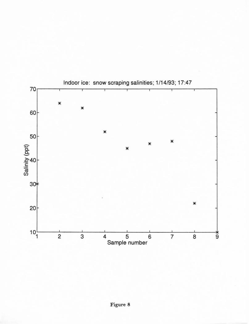
Indoor ice: snow scraping salinities ; 1 /14/93; 17:47

60 ,_ -

50-- -

-+-' c. c. -.~40- -c ro

Cf)

30~ -

20 - -

I I I I I I I

2 3 4 5 6 7 8 9 Sample number

F igure 8

Indoor ice : snow scraping salinities; 1 /1 5/93 ; 11 :30 72 I I I I I

70 -- -

68-- -

66-- -

--c.. c..64-- -->..

.-:= c

:.= 62 - -ca Cf)

60 - -

58 - -

56 -- -

54 I ' I I I •

2 4 6 8 10 Sample number

Figure 9

25

24

23

22

,....,. 21 .... 0.. 5

1

18

1

16

1

.. ··I

I .; .;

.;

. ,, J,. .;

.; . "' "' I

1.5

I ' '

-* / ·

I

I

*

2

1/28; Pond ice; near surface salinities

' '

'

I I

I . .I , ..

I

' '

' I I

I I

I I

I I

I , snow-roughened ice

I ' I

I I

I

2.5

' ·'. snow-roughened ice ' '

smooth i

* · ·· · · · ··· · · · ······ · ···· l*:

3 Depth (mm)

snow-roughened ice

3.5 4

Figure 10

4.5 5

20

18

1

12

1

1/29; morning and afternoon; pond ice near surface salinities

smooth ice

____ _ ·:::, _____ ""*'

~ ';;..- . '*-.-~----~---....

snow-roughened ice ' .... , ' ' ' *" ' t '

1.5 2

' '

2.5

'

3 Depth (mm)

Figure 11

...

3.5

... . . ·~IE' . . ,,, ,,, ,,, ,,, ,,, ,,, ,,, ,..JI(

4

,,, ,,,

. ;.-.. . / . · ,,, .· ,,,

,,, ,,, ,,,

4.5 5

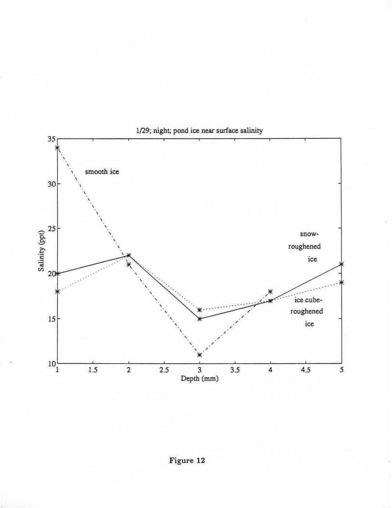
1/29; night; pond ice near surface salinity

'

' smooth ice

30

' ' '

- 25 ..... 0.. & 0

' \. snow-

' roughened

~ ice

Cl) 2 '

' '

' ' ice cube-

' ' roughened

' /

/ ice ' /

15

' /

' /

\. /

' /

* lQ'--~~--L~~~---'-~~~-'-~~~-L-~~~..__~~--'~~~---'-~~~--'

1 1.5 2 2.5 3 3.5 4 4.5 5 Depth (mm)

Figure 12

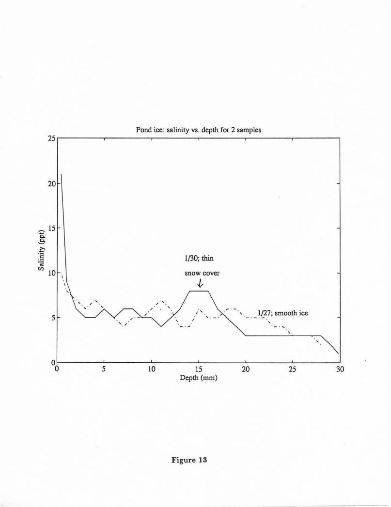
20

- 15 ...... 0.

-9: 0 ·a ~ Cl) 10

5

0 0 5

Pond ice: salinity vs. depth for 2 samples

1/30; thin

snow cover

,. ' . 1/27; smooth ice

' '

'

10 15 20 25 30 Depth (mm)

Figure 13

,... p 28 lot E 1 - 4 u c: s lg,,, 0 . 3916 Cfll 0

..., ..., ..c 0 . 5 ~ 3 tn .0

., " J: ...,

2 0 " "d ... ., "d

N +' ... -0 . 5 1 - ..i:;

IC tn E ., " 0 -1 ::c 0 z: 0 100 200 300 -1 - 0 . 5 0 0.5 1

Horizontal distance ( ,,,,,, ) Height (c,,,' nor,,,. to 0 ,,,ean)

1 1 Fit to autocorr. f u nc .

po l yno,,,,

0.8 CCR) exp,

8 .5 Gss. ,... 0.6 po In,,,.

Ill; Ill; ..... ..... u

8 u 8.4

0.2

-ELS El 8 100 200 300 0 10 20 30 40

R ( ,,,,,, ) R ( ,,,,,, )

Jn<loor ice with ice cubes, afler 2nd spraying (1/18/93)

Figure 14

Optical measurements: Optical measurements were made in conjunction with the outdoor pond studies. All-wave radiometers were used to routinely monitor incident, reflected. and transmitted total shortwave irradiance. In addition, spectral albedos were measured at selected times during the growth of the ice sheet, and the subsequent snowfall, and also of the roughened and unroughened surfaces. The spectral albedo measurements were closely coordinated with the passive microwave program (Grenfell). Figure I is a photograph

showing the pond with a 3 cm thick ice cover. The upward and downward looking all­wave radiometers are in the foreground and the tripod-mounted spectroradiometer is in the background. An ice sample was taken at each spectral albedo measurement to ascertain the physical properties of the ice. This characterization included determining vertical profiles of temperature, salinity and brine volume and preparing ice thin sections for an analysis of the inclusion size distribution.

Spectral albedos for thin growing ice and for snow covered ice are plotted in Figure 2. There was an gradual increase in albedo at all wavelengths as the ice grew thicker. The maximum albedo for the bare ice was at approximately 550 nm. We believe that this was due in part to the contribution of the underlying water,

1.0 ..---..---..,..---.--"""'T""---.-----.

0.8

0.6

13 snow, 8.2 Ice ---'•-,, . .,,¥\~\~

0.5 cm snow, 8.2 cm Ice

---------------------------------~ which had a dark-green hue. The presence .g of even a thin snow cover (0.5 cm) caused ~ a sharp increase in albedo at all <e o.4 8.2

.,,;;:~···-· -.......• wavelengths. For a snow depth of 13 cm, albedos were greater than 0. 9 and the snowcover was optically thick. 0.2

,;:;- ,/ 6.2 --------~ ,/" ..---:.~'--,~,-­

- 5.2

3. 1 cm

0.0 ....___...___......__........_ _ _..._ _ __.__~

400 600 800 1000

Wavelength (nm)

Indoor pit 0 ..----.----..--~---,..--~---..,ro----r=-~

~---0

4

...--... E ~ 8 ..c: ..... a. Q)

0

12

0 0

11 -•-10Jan -0-12Jan

? ."" \ ·~ 0 • I

0

I 0 I

0 \ 0 \ o"' /0

0

\ 0

Outdoor pond

-•-21 Jan - 0 - 3Feb

4

0 CD

"'C as: ...--... 0 3 ..........

12

16 ._.......__.._ ......... _..._ ......... _.___ ---------------- 16 0 5 10 15 20 0 5 10 15 20

Salinity (o/oo) Salinity (o/oo)