Laboratory Investigation of Radial Flow Dynamics
101
Laboratory Investigation of Radial Flow Dynamics Thomas Gallop
Transcript of Laboratory Investigation of Radial Flow Dynamics
Laboratory Investigation of
Radial Flow Dynamics
Thomas Gallop

Laboratory Investigation of Radial Flow Dynamics
Page 2
Acknowledgements
Work on this project has taken up the best part of a year of my life and now that is
completed I realise that what I have achieved would not have been possible without great
support from the people around me.
Firstly I would like to thank Dr. Prabhakar Clement for being a great supervisor and
providing the inspiration and enthusiasm required for this project. At same time I would
like to acknowledge the work of Matthew Simpson, whose amazing patience and support
throughout the year made the work so much easier.
Also worthly of thanks is the group of final students from the Centre for Water Research.
Studying with you guys over the past year has been an absolute pleasure and I wish you
all the best of luck for the future. At the same time I wish to acknowledge all my friends
outside of department for their constant support. I am in debt to all of you.
Last, but not least I wish to acknowledge my family, Dad, Mum and Leo for providing so
much support throughout the year. I realise that I have not been the easiest person to live
with and I thank you all for your patience and inspiration.
Laboratory Investigation of Radial Flow Dynamics
Page 3
Abstract
An understanding of unconfined radial flow is crucial for predicting the flow dynamics of
groundwater systems. Two theories used to simulate unconfined radial flow are the
Dupuit-Forchheimer flow model and the variably-saturated flow model. Simplifying
assumptions allow the Dupuit-Forchheimer flow model to reduce the governing flow
equation to an ordinary differential equation that can be solved analytically; while
solution of the variably-saturated flow model requires numerical approximation of a non-
linear partial differential equation.
Using a physical model of a radial flow system, head differentials were set up and
measurements were taken of travel time, flow, streamlines and pressure heads. These data
sets were compared to the predictions of the two flow models described above.
Measurement of particle travel times using dye showed that travel times for dye reaching
a downstream well increased as the height of release at the upstream boundary was
increased. This phenomenon is caused by the increase in the length of travel paths as the
height of release is increased together with the fall in average flow velocities with
increasing height. The Dupuit-Forchheimer flow model assumes that there should be no
variation in travel times with height. For the systems considered here this assumption
does not hold, with the Dupuit-Forchheimer model underestimating the actual travel
times with an average error of 140%. The variably-saturated flow model on the other
hand was found to give a good approximation to the actual travel times with an average
error of 8%. Measurement of travel times also enabled the observation of downstream
velocity profiles for the radial flow system. The profiles showed a general increase in
flow velocity moving down the downstream end, reaching a maximum value at the height
of the downstream well and then decreasing.

Laboratory Investigation of Radial Flow Dynamics
Page 4
Contents
1.0 LITERATURE REVIEW .................................................................................................................... 9
2.0 INTRODUCTION............................................................................................................................... 20
3.0 METHODS .......................................................................................................................................... 21
3.1 TANK PREPARATION......................................................................................................................... 21
3.1.1 Tank Screens ............................................................................................................................... 24
3.1.2 Porous Medium ........................................................................................................................... 25
3.2 SATURATED HYDRAULIC CONDUCTIVITY ....................................................................................... 25
3.3 PHYSICAL MEASUREMENTS ............................................................................................................. 27
3.3.1 Steady-State Conditions.............................................................................................................. 27
3.3.2 Flow............................................................................................................................................. 30
3.3.3 Travel times ................................................................................................................................. 30
3.3.4 Downstream velocity profile....................................................................................................... 32
3.3.5 Streamlines .................................................................................................................................. 33
3.3.6 Potentiometric levels................................................................................................................... 34
3.4 NUMERICAL MODELS........................................................................................................................ 34
3.4.1 Variably-saturated flow equation............................................................................................... 34
3.4.2 Dupuit-Forchheimer flow equation: Evaluation of travel times............................................... 35
4.0 ANALYSIS AND SYNTHESIS......................................................................................................... 36
4.1 SATURATED SAND HYDRAULIC CONDUCTIVITY............................................................................. 36
4.2 FLOW................................................................................................................................................. 36
4.2.1 Variably-saturated flow .............................................................................................................. 37
4.2.2 Analysis of physical results......................................................................................................... 38
4.3 TRAVEL TIMES .................................................................................................................................. 42
4.4 DOWNSTREAM VELOCITY PROFILE................................................................................................... 56
4.5 STREAMLINES ................................................................................................................................... 60
4.6 POTENTIOMETRIC LEVELS................................................................................................................ 68
5.0 CONCLUSIONS ................................................................................................................................. 74
6.0 RECOMMENDATIONS ................................................................................................................... 76
7.0 REFERENCES.................................................................................................................................... 77

Laboratory Investigation of Radial Flow Dynamics
Page 5
APPENDIX A: NUMERICAL MODEL OF TWO-DIMENSIONAL, VARIABLY-SATURATED
FLOW.................................................................................................................................................................. 80
A.1 BOUNDARY CONDITIONS.................................................................................................................. 81
A.2 SOIL PROPERTIES.............................................................................................................................. 84
APPENDIX B: RADIAL FLOW MODEL PLANS ...................................................................................... 86
APPENDIX C: MEASURING SATURATED HYDRAULIC CONDUCTIVITY ................................... 92
APPENDIX D: PHYSICAL RESULTS.......................................................................................................... 95
Laboratory Investigation of Radial Flow Dynamics
Page 6
Figures
Figure 1: Confined and unconfined aquifer flow (Fetter, 1994)........................................9
Figure 2: Phreatic surfaces predicted by the Dupuit-Forchheimer and variably-saturated
flow models (Modified from Clement et al. (1996)) ...............................................13
Figure 3: Velocity distributions along the outflow face of a two-dimensional radial flow
system (Muskat, 1937)...........................................................................................15
Figure 4: Top view of system under consideration. ........................................................22
Figure 5: Piezometer positions (all values in cm). ..........................................................23
Figure 6: Analysis grid for tank (r = distance from upstream end, z = elevation) ............24
Figure 7: Constant Head Permeameter...........................................................................26
Figure 8: Falling Head Permeameter..............................................................................27
Figure 9: Time for achievement of steady state. .............................................................29
Figure 10: Pore drainage areas for different head gradients ............................................30
Figure 11: Dye traveling through radial tank..................................................................32
Figure 12: Flow observed at different head differentials with hydraulic conductivity of 48
m/day (upstream head = 90cm) ..............................................................................39
Figure 13: Flow rate predictions using a saturated hydraulic conductivity of 67m/day. ..41
Figure 14: Dye released at heights of 80cm, 50cm and 20cm for a 90:10 head gradient .43
Figure 15: Total travel times for 90:20 head differential ................................................44
Figure 16: Total travel times for 90:40 head differential ................................................44
Figure 17: Total travel times for 90:60 head differential ................................................45
Figure 18: Total travel times for 90:70 head differential ................................................45
Figure 19: Comparison of total travel times for changing head differentials ...................46
Figure 20: Comparison of total travel times for dye released at 90cm and dye released at
15cm......................................................................................................................47
Figure 21: Predicted travel times for four head differentials together with their quadratic
curves of best fit ....................................................................................................51
Figure 22: Dye travel times for 90:20 head differential through tank at different heights of
release ...................................................................................................................53
Laboratory Investigation of Radial Flow Dynamics
Page 7
Figure 23: Dye travel times for 90:40 head differential through tank at different heights of
release ...................................................................................................................54
Figure 24: Dye travel times for 90:60 head differential through tank at different heights of
release ...................................................................................................................55
Figure 25: Dye travel times for 90:70 head differential through tank at different heights of
release ...................................................................................................................56
Figure 26: Observed downstream velocities for the 90:10 head differential....................57
Figure 27: Observed downstream velocities for the 90:75 head differential....................58
Figure 28: Correct pump and treat design ......................................................................60
Figure 29: Streamlines observed for the 90:20 head differential.....................................61
Figure 30: Streamlines observed for the 90:40 head differential.....................................62
Figure 31: Streamlines observed for the 90:60 head differential.....................................63
Figure 32: Streamlines observed for 90:70 head differential...........................................64
Figure 33: Streamlines observed for a 90:10 head differential........................................65
Figure 34: Seepage face heights for upstream well height of 90cm ................................67
Figure 35: Piezometric levels for the 90:20 head differential..........................................69
Figure 36: Piezometric levels for the 90:40 head differential..........................................70
Figure 37: Piezometric levels for the 90:60 head differential..........................................71
Figure 38: Piezometric levels for the 90:70 head differential..........................................72
Laboratory Investigation of Radial Flow Dynamics
Page 8
Tables
Table 1: Observed and measured flow rates for various head differentials .....................37
Table 2: Flow rate predicted by variably-saturated flow model at different grid sizes for a
90:75 head differential ...........................................................................................38
Table 3: Factor of difference between observed flow and predicted flow from the
variably-saturated flow model................................................................................40
Table 4: Percentage errors in flow measurements for Dupuit-Forchheimer and variably-
saturated flow models ............................................................................................41
Table 5: Comparison of errors in travel times predicted by the variably-saturated flow
model and those physically observed. ....................................................................49
Table 6: Comparison of travel times predicted by the Dupuit-Forchheimer flow model
and those physically observed. ...............................................................................50
Table 7: Comparison of observed travel times with those predicted by an empirical
relation. .................................................................................................................52

Laboratory Investigation of Radial Flow Dynamics
Page 9
1.0 Literature Review
The flow of groundwater towards a pumping well can be divided into two main areas:
confined aquifer and unconfined (gravity) aquifer flow.
Figure 1: Confined and unconfined aquifer flow (Fetter, 1994)
Confined aquifer flow applies to the flow of water between two confining layers (Figure
1). The distance between the confining layers governs saturated thickness of the confined
flow, with the porous medium between the layers being completely saturated.
Unconfined aquifer flow on the other hand applies to flow with only a single confining
layer at the base of the aquifer. As a result this makes the study of unconfined flow more
complex as the saturated thickness of the porous medium can vary spatially. Unconfined
aquifer flow also enables the occurrence of unsaturated flow above the saturated area of
the aquifer. Due to these factors unconfined flow exhibits a non-linear nature, which
Laboratory Investigation of Radial Flow Dynamics
Page 10
leads to complex governing equations that are difficult to solve. Accurate solutions
however are often necessary as unconfined flow is the most commonly occurring flow in
nature. Therefore a greater understanding of unconfined flow is required for
understanding problems involving groundwater contamination.
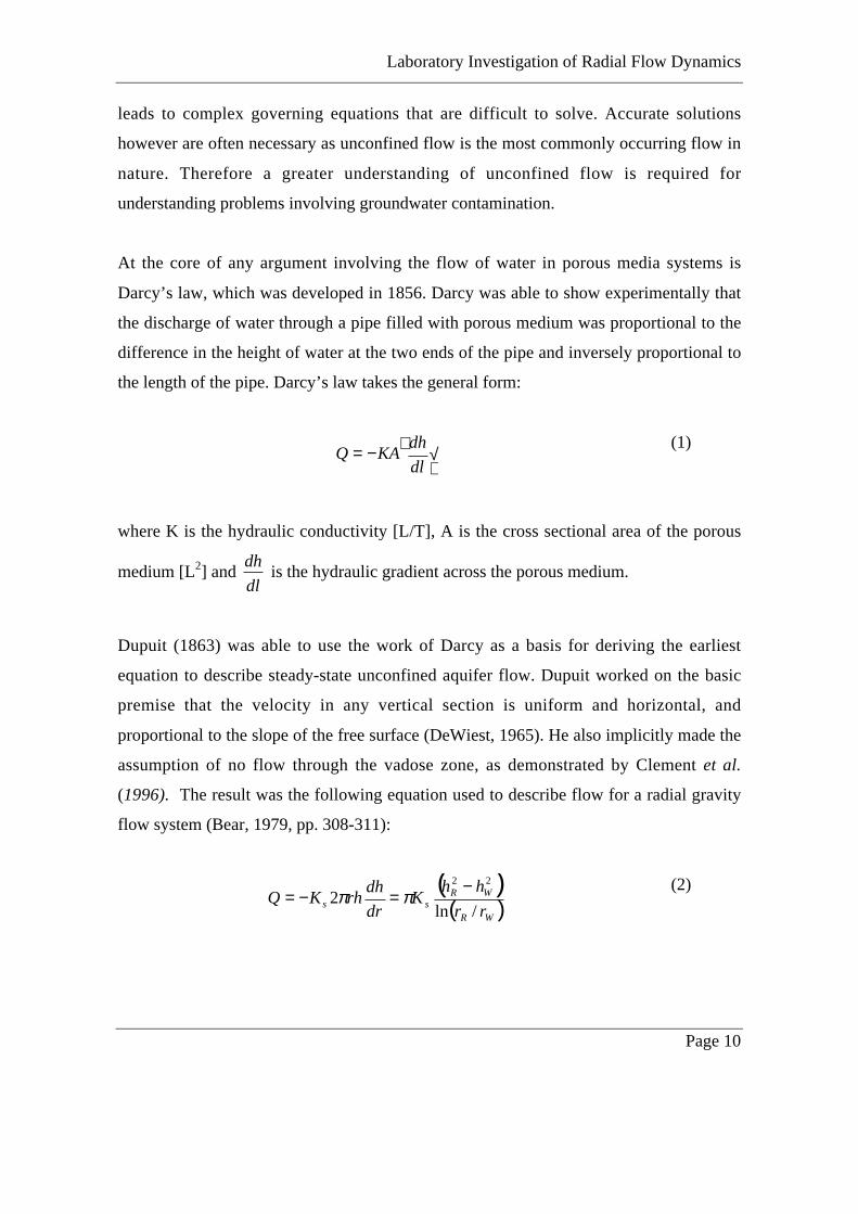
At the core of any argument involving the flow of water in porous media systems is
Darcy’s law, which was developed in 1856. Darcy was able to show experimentally that
the discharge of water through a pipe filled with porous medium was proportional to the
difference in the height of water at the two ends of the pipe and inversely proportional to
the length of the pipe. Darcy’s law takes the general form:
√↵
−=dl
dhKAQ
(1)
where K is the hydraulic conductivity [L/T], A is the cross sectional area of the porous
medium [L2] and dl
dh is the hydraulic gradient across the porous medium.
Dupuit (1863) was able to use the work of Darcy as a basis for deriving the earliest
equation to describe steady-state unconfined aquifer flow. Dupuit worked on the basic
premise that the velocity in any vertical section is uniform and horizontal, and
proportional to the slope of the free surface (DeWiest, 1965). He also implicitly made the
assumption of no flow through the vadose zone, as demonstrated by Clement et al.
(1996). The result was the following equation used to describe flow for a radial gravity
flow system (Bear, 1979, pp. 308-311):
( )( )WR
WRss rr
hhK
dr
dhrhKQ
/ln2
22 −=−= ππ
(2)
Laboratory Investigation of Radial Flow Dynamics
Page 11
where Q [L3T-1] is the total discharge through the system with boundary conditions, hw
[L] the water table elevation at the radius of the well, rw [L], and hR [L] the height of the
water table at the radius of influence, rR [L]. Integration of equation (2) yields:
( ) ( ) ( )( )
2/1
222
/ln
/ln(
??−+=
WR
wWRW rr
rrhhhrh
(3)
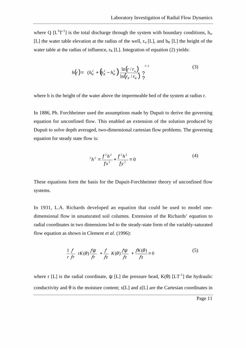
where h is the height of the water above the impermeable bed of the system at radius r.
In 1886, Ph. Forchheimer used the assumptions made by Dupuit to derive the governing
equation for unconfined flow. This enabled an extension of the solution produced by
Dupuit to solve depth averaged, two-dimensional cartesian flow problems. The governing
equation for steady state flow is:
02
22
2
2222 =
ƒƒ+
ƒƒ=
y
h
x
hh
(4)
These equations form the basis for the Dupuit-Forchheimer theory of unconfined flow
systems.
In 1931, L.A. Richards developed an equation that could be used to model one-
dimensional flow in unsaturated soil columns. Extension of the Richards’ equation to
radial coordinates in two dimensions led to the steady-state form of the variably-saturated
flow equation as shown in Clement et al. (1996):
0)(
)()(1 =++
z
K
zK
zrrK
rr ƒθƒ
ƒƒψθ
ƒƒ
ƒƒψθ
ƒƒ (5)
where r [L] is the radial coordinate, ψ [L] the pressure head, K(θ) [LT-1] the hydraulic
conductivity and θ is the moisture content; x[L] and z[L] are the Cartesian coordinates in

Laboratory Investigation of Radial Flow Dynamics
Page 12
the horizontal and vertical directions respectively. This equation assumes that the
dynamics of the air phase do not affect those in the water phase, the density of the water
is only a function of the pressure and the spatial gradient of the water density is
negligible.
The variably-saturated flow equation (5) allows for both vertical variation in pressure (as
zƒƒ
is non-zero), and changes in unsaturated hydraulic conductivity (as K = K(θ)). As a
result, this approximation avoids the assumptions used in the Dupuit-Forchheimer model.
The solution of the variably-saturated flow equation leads to the development of seepage
face at the downstream end of the model. The seepage face refers to the area at the
downstream face between the intersection of the phreatic surface at the downstream end
of the domain and the water level in the downstream well, where the water pressure is
atmospheric (Clement et al., 1994). Figure 2 compares the phreatic surfaces predicted by
the two models, showing the formation of a seepage face in the variably-saturated flow
model.
Laboratory Investigation of Radial Flow Dynamics
Page 13
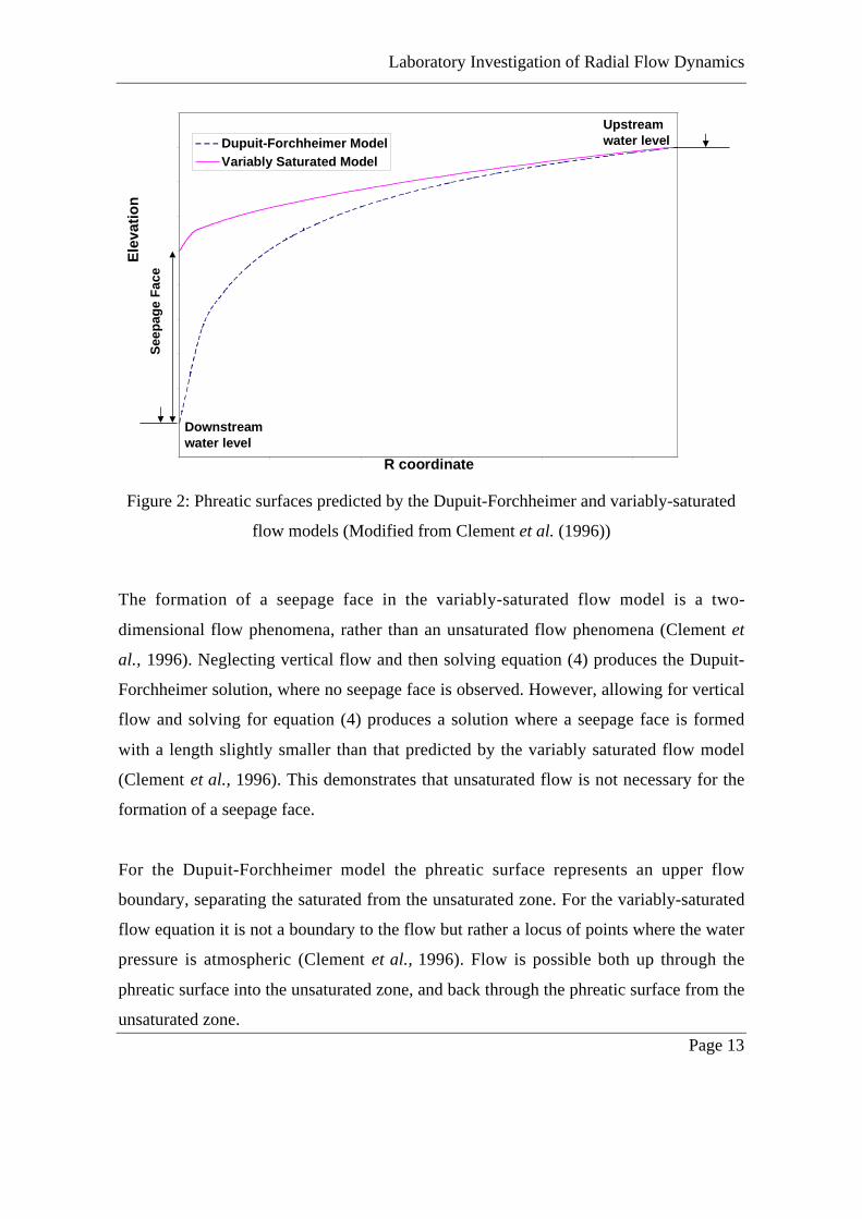
Figure 2: Phreatic surfaces predicted by the Dupuit-Forchheimer and variably-saturated
flow models (Modified from Clement et al. (1996))
The formation of a seepage face in the variably-saturated flow model is a two-
dimensional flow phenomena, rather than an unsaturated flow phenomena (Clement et
al., 1996). Neglecting vertical flow and then solving equation (4) produces the Dupuit-
Forchheimer solution, where no seepage face is observed. However, allowing for vertical
flow and solving for equation (4) produces a solution where a seepage face is formed
with a length slightly smaller than that predicted by the variably saturated flow model
(Clement et al., 1996). This demonstrates that unsaturated flow is not necessary for the
formation of a seepage face.
For the Dupuit-Forchheimer model the phreatic surface represents an upper flow
boundary, separating the saturated from the unsaturated zone. For the variably-saturated
flow equation it is not a boundary to the flow but rather a locus of points where the water
pressure is atmospheric (Clement et al., 1996). Flow is possible both up through the
phreatic surface into the unsaturated zone, and back through the phreatic surface from the
unsaturated zone.
R coordinate
Ele
vati
on
Dupuit-Forchheimer Model
Variably Saturated ModelS
eep
age
Fac
e
Downstream water level
Upstream water level

Laboratory Investigation of Radial Flow Dynamics
Page 14
The Dupuit-Forchheimer model has a distinct advantage in that the equation used to
model the flow is one dimensional and can be solved analytically. On the other hand, the
variably-saturated flow equation is a non-linear partial differential equation, where
analytical solutions cannot be produced. The Dupuit-Forchheimer model also has the
advantage of easily identifiable boundary conditions, with only upstream and
downstream water levels required. Boundary conditions for the variably-saturated flow
equation are not clearly identifiable as the height of the seepage face is unknown. The
variably-saturated flow equation however is more accurate, especially in conditions
where vertical flows and flow in the unsaturated zone become important. These
conditions are generally produced by large hydraulic gradients in a porous medium that
exhibits strong capillary effects.
Wyckoff et al. (1932) conducted an experiment using the sector of a radial tank to gain a
greater understanding of radial flow. The authors used the tank to show that outflow is
proportional to the square of the differences in fluid heads (as measured from the tank
bottom). The Dupuit formula gives a similar result with fluid heads replaced by phreatic
surface heights. Some findings were also made that contradicted the assumptions of the
Dupuit formula. The authors were one of the first to observe the formation of a seepage
face, with the size of the seepage face increasing as the upstream height was increased. A
reduction in fluid head, when compared to fluid level, at the downstream end of the
model highlighted seepage face formation. Streamlines from the model also showed that
significant vertical flow was present which further contradicted the Dupuit-Forchheimer
assumptions. At the upstream end, flow moved upwards into the capillary zone while at
the downstream end, downward flow out of the capillary zone was observed. Under
conditions where the capillary zone was large it was found that the Dupuit-Forchheimer
model for predicting flow was in fact incorrect and an extra term for capillary flow was
required to describe the flow. The introduction of this extra term into the Dupuit flow
equation (2) is highlight in equation (6):
Laboratory Investigation of Radial Flow Dynamics
Page 15
( )( )( )WR
CWRWRs rr
hhhhhKQ
/ln
++−=π
(6)
where hc was the capillary rise of the fluid. The observation of seepage faces, vertical and
capillary flow highlighted the deficiencies of some of the Dupuit-Forchheimer
approximations and that further work in the area was required.
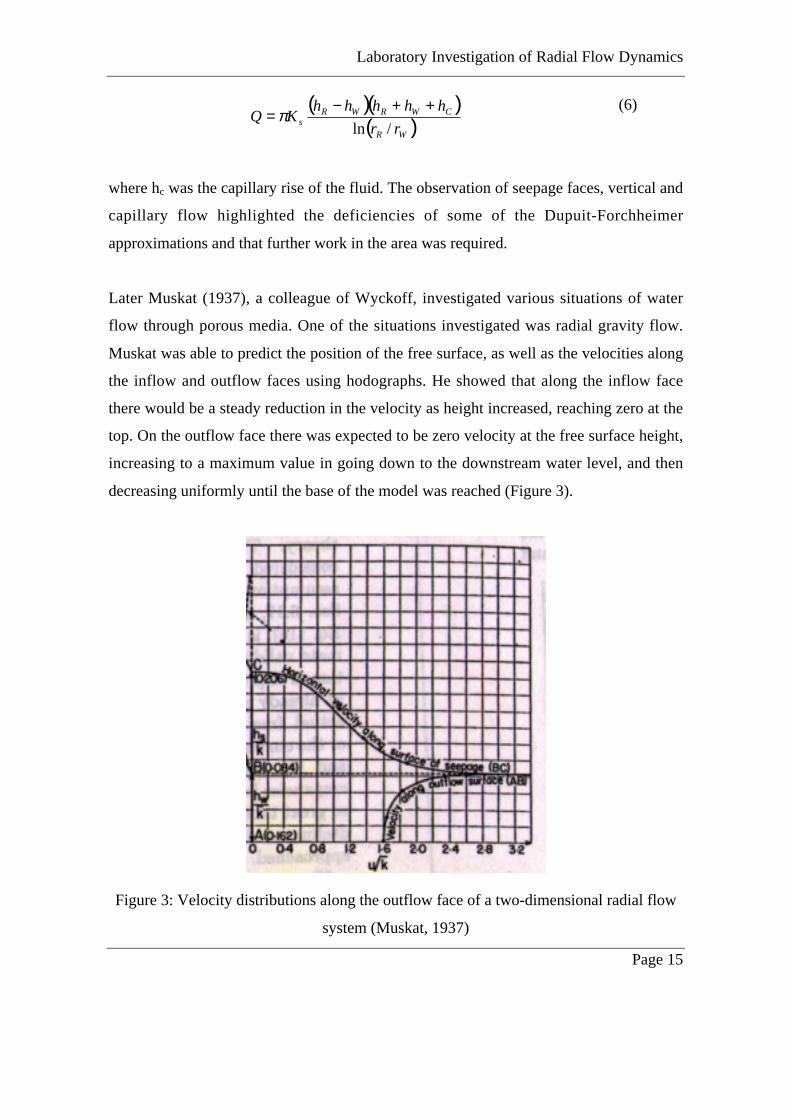
Later Muskat (1937), a colleague of Wyckoff, investigated various situations of water
flow through porous media. One of the situations investigated was radial gravity flow.
Muskat was able to predict the position of the free surface, as well as the velocities along
the inflow and outflow faces using hodographs. He showed that along the inflow face
there would be a steady reduction in the velocity as height increased, reaching zero at the
top. On the outflow face there was expected to be zero velocity at the free surface height,
increasing to a maximum value in going down to the downstream water level, and then
decreasing uniformly until the base of the model was reached (Figure 3).
Figure 3: Velocity distributions along the outflow face of a two-dimensional radial flow
system (Muskat, 1937)

Laboratory Investigation of Radial Flow Dynamics
Page 16
Muskat explained how despite the obvious limitations of the Dupuit approximations, the
Dupuit-Forchheimer formula still led to a reasonable calculation of the total flow rate for
the system, thus attempting to explain the observations of Wycoff et al. (1932). He
achieved this by using the same boundary conditions as Dupuit but without the free
surface boundary. Muskat also described an experiment undertaken by Wycoff et al.
(1935) where this gravity flow system was modelled using an electric circuit. The model
supported what had earlier been observed in the laboratory, with the formation of large
seepage faces and significant vertical velocities.
In 1955, Hall used modelling procedures similar to those used by Wycoff et al. (1932) to
conduct a series of physical experiments. Hall particularly concentrated on observation
close to the downstream gravity well of the system where the slope of the free surface
becomes steep and the Dupuit-Forchheimer assumptions are expected to be invalid. Hall
observed the formation of streamlines in the tank and took pressure readings from
piezometers connected to the tank. From this data he was able to produce flow patterns
for each head gradient showing streamlines and equipotential lines. Hall’s results were
used to validate numerical results produced by a relaxation method. This method used
equation (4) to define a pair of empirical equations that may be used to locate the phreatic
surface on a typical radial cross section. The method however did not account for
capillary effects. Hall was the first to physically observe a reduction in travel time with
falling height of release. He also noted that travel times for dyes released in the capillary
layer were considerably slower than those just slightly below this zone. Some rough
measurements of travel time were taken however these results were only extensive
enough for qualitative analysis. These velocities however did enable Hall to make
estimations of the contribution of the capillary layer relative to the total flow.
From the physical observations of Wycoff et al. (1932) and Hall (1955) it was clear that
the Dupuit-Forchheimer formula could be inaccurate at the downstream end of the flow
problem due to the formation of a seepage face. Borelli (1955) investigated situations
where the Dupuit-Forchheimer model could still be used accurately. By comparing
Laboratory Investigation of Radial Flow Dynamics
Page 17
results gained from the relaxation method with those of Dupuit-Forchheimer, he was able
to estimate a ratio for radius r to the height of the phreatic surface h (see Figure 1 for
unconfined aquifer), above which the Dupuit-Forchheimer model would predict the
position of the phreatic surface to within 1%. Using this estimate he developed a formula
to calculate the position of the phreatic surface at positions closer to the downstream
well, where the Dupuit-Forchheimer assumptions are not valid. This approach however
has limited use as it is related to a particular flow system.
Emphasis on modelling the variably-saturated flow equation (5) using numerical schemes
was instigated by Rubin (1968). Rubin used a finite difference method to solve the two-
dimensional variably-saturated flow equation. Other work included that of Neuman
(1973), who used a finite element approach to solve the two-dimensional variably-
saturated flow equation. Narasimhan and Witherspoon (1976) used an integrated finite
difference method, while Cooley (1983) used a sub-domain finite-element approach to
solve a similar flow problem.
Vachaud and Vauclin (1975) performed a series of laboratory experiments on a cartesian
flow tank. By combining measurements from pressure transducers on the tank with
Darcy’s Law they were able to measure water fluxes in the system. From these results
they observed a downstream velocity profile similar to that predicted by Muskat (1937).
Shamsai and Naraisimhan (1991) used a numerical model for the variably-saturated flow
equation, previously developed by Naraisimhan and Witherspoon (1978), to model some
of the experimental observations documented by Hall (1955). The model was found to be
accurate in calculating the phreatic surface and the distribution of potentials within the
phreatic zone observed by Hall (1955). Work was also undertaken to compare the
discharge levels observed by the model with those estimated by the Dupuit-Forchheimer
model under different situations. The results showed that discharge estimates from the
Dupuit-Forchheimer model were in error by up to 12-20% for both radial and cartesian
flow situations. These are much higher levels than the 1-2% predicted by several other

Laboratory Investigation of Radial Flow Dynamics
Page 18
investigators including Muskat (1937), thus indicating that one cannot always neglect the
role of the unsaturated zone when dealing with unconfined flow problems.
Clement et al. (1994) developed a numerical algorithm capable of solving a variety of
two-dimensional, variably-saturated flow problems. Details of this numerical model are
included in Appendix A. The model was shown to accurately predict several known
experimental data sets, including the water table data observed by Hall (1955).
Clement et al. (1996) compared the effectiveness of different models for predicting
steady state, unconfined flow for different soil properties, problem dimensions and flow
geometries. Using a previously developed numerical model (Clement et al., 1994) a
comparison of results produced by the Dupuit-Forchheimer equation and the variably-
saturated flow equation was completed. Observations showed that the position of the
phreatic surface was relatively insensitive to the soil parameters used in the variably-
saturated flow equation. This explains why the experiment conducted by Hall (1955) was
reproducible by numerical means e.g. Shamsai and Naraisimhan (1991), despite the fact
that Hall did not report any soil parameters. Comparison of radial to cartesian problems
revealed that the effect of flow through the vadose zone is relatively less important in
radial than in cartesian systems. The radial flow case was also found to produce a more
pronounced seepage face. This can be explained by the convergent nature of radial flow,
where a larger seepage area is required to accommodate the induced flow. The radial
flow problem was much less sensitive to changes in the scale of the model compared to
cartesian flow problems, highlighting the persistent nature of seepage faces in radial flow
problems.
The literature indicates that although extensive study has been undertaken in the area of
radial unconfined flow, further investigation is still required, particularly in relation to the
observation of flow velocities and internal flow patterns near a seepage face boundary. It
has been observed by Hall (1955) that travel times increase with increasing height of
release, however this observation was made from only qualitative results for a simple
case. The opportunity is therefore present for quantitative physical study of the travel

Laboratory Investigation of Radial Flow Dynamics
Page 19
times in a radial flow situation. The Dupuit-Forchheimer model for radial flow systems
predicts that the travel times observed should be independent of height of release.
Detailed observation of travel times over a number of head differentials will enable the
extent to which this assumption fails to be physically documented. Measurement of travel
times will also allow measurement of the downstream velocity profile. This typical
profile shown in Figure 3 has been observed in a physical cartesian system however it has
never been observed physically in a radial system. Comparison of the results with those
predicted by a numerical model will help validate the effectiveness of the model to
predict flow velocities for an unconfined radial flow system. A greater understanding of
unconfined radial flow will lead to a greater understanding radial flow dynamics, thus
allowing for the implementation of more efficient pumping practices.
Laboratory Investigation of Radial Flow Dynamics
Page 20
2.0 Introduction
This study focused on the physical observation of flow through a two-dimensional radial
system. This involved using a radial tank and experimental design developed by Matthew
Simpson for the Centre for Water Research as part of his PhD thesis. The design details
of the tank are included in Appendix B.
This tank allowed a constant head differential to be set up between the two ends of the
system so that steady state flow conditions could be achieved. At this stage observation
of travel times, streamlines, and pressure levels at various positions in the tank took
place, together with a measure of total flow through the tank. The process was repeated at
a number of head differentials. A comparison of these results with those from the
numerical model for variably-saturated flow (Appendix A) will enable further
understanding of unconfined flow near a seepage face boundary.
The laboratory efforts were focused on observing travel times for flow in the tank.
Observation of changing travel times with height of release had been insufficient in
previous studies, and quantitative physical observation was required to validate much of
the seepage face theory, including that of Clement et al. (1996). Some study also focused
on measuring a downstream velocity profile, and comparing it to the theoretical profile.

Laboratory Investigation of Radial Flow Dynamics
Page 21
3.0 Methods
3.1 Tank Preparation
The model used to observe flows was a 15o cut of a radial system with a height of 100 cm
and distance between well centres of 129.56 cm (Simpson, 2000). The 15o cut was
assumed to represent a portion of a complete radial flow system. The model was divided
into three chambers: the inlet flow chamber (or upstream well), the porous medium and
the outlet flow chamber (or downstream well). The internal diameter of the upstream well
was 20 cm and the internal diameter of the downstream well was 10 cm. This enabled the
investigation of a convergent radial flow situation. The model used was constructed of
pexiglass with a metal frame attached to avoid deflection of the sidewalls. Two Pexiglass
screens were used at the upstream and downstream ends to hold in the sand medium.
Although we assume that the system we are considering is radial, this is not completely
true due to the presence of flat screens (Figure 4). However, this is an adequate
assumption as the small value chosen for the angle of the cut (15o) means that the
difference from the ideal system is also small.

Laboratory Investigation of Radial Flow Dynamics
Page 22
Figure 4: Top view of system under consideration.
Flow of water into the tank was controlled via a hose connected to the mains water
supply. Water outflow was controlled by poly vinyl chloride (PVC) pipes present in the
upstream and downstream wells. Water was able to flow out of the pipes and into the
drain via tubing connected to the bottom of the pipe. Connections at the bottom of the
tank allowed these pipes to be moved up and down in the wells, thus controlling the
water levels in the upstream and downstream ends of the tank. A valve was also present
at the bottom of the tank allowing the water flow through these pipes to be stopped at any
time.
10cm
Model system
True radial flow system
109.5cm

Laboratory Investigation of Radial Flow Dynamics
Page 23
One side of the tank contained holes drilled such that plastic piping could be attached.
These holes were covered with small pieces of geofabric on the inside of the tank to
prevent sand from entering the piping. Each piece of piping acted as a piezometer
enabling the measurement of pressure heads in the tank. Figure B3 (Appendix B) shows
the piezometers on the side of the tank and Figure 5 shows their positions relative to the
upstream and downstream wells.
Figure 5: Piezometer positions (all values in cm).
Ups
trea
m w
ell s
cree
n
Dow
nstr
eam
wel
l scr
een
15.5 20 20 19.5 20 15
5
20
20
20
15
15
125
125
Side View
Top View

Laboratory Investigation of Radial Flow Dynamics
Page 24
On the other side of the tank the glass area was divided into a grid with squares 5 cm × 5
cm (Figure 6). The grid enabled easier monitoring of the streamlines and flow velocities
in the tank.
z
r
4070 105
Figure 6: Analysis grid for tank (r = distance from upstream end, z = elevation)
3.1.1 Tank Screens
The sand was held within the tank by two pexiglass screens, with holes drilled at regular
intervals to allow the flow of water through the screens. The design of the screens is seen
in Figure B4 (Appendix B). The holes were positioned such that the screen had maximum
strength, and that water could enter and exit the tank at all heights along the screen. The

Laboratory Investigation of Radial Flow Dynamics
Page 25
screens were wrapped initially with a rubber mesh and then with geofabric to prevent the
movement of porous media into the upstream and downstream ends of the tank.
3.1.2 Porous Medium
The porous medium used to pack the radial tank was a 1±0.5 mm medium sand (Cook
Industrial Minerals Pty. Ltd.). The sand was added to the tank in layers of ~2 cm with the
water level always maintained above that in the sand. After each addition, the sand in the
tank was mixed thoroughly using a piece of PVC piping, allowing for removal of air
bubbles trapped in the sand pores. This was continued until the height of the sand in the
tank was 95 cm. So as to prevent air bubbles from entering the porous media and
disrupting the results between experimentation, the water level in the tank was
maintained above the height of the sand. After packing the tank with porous medium it
was also noted that significant deflection of the upstream well screen into the upstream
well occurred. As a result, the system in the model moved closer to the true radial flow
system described in Figure 4.
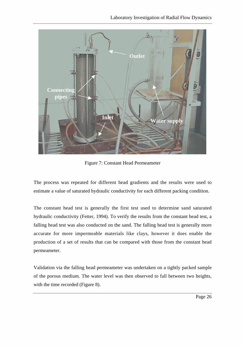
3.2 Saturated Hydraulic Conductivity
The saturated hydraulic conductivity of the porous medium was measured using a
constant head test. Two sets of sand packing conditions were used, one where the sand
was packed tightly and one where no attempt was made to pack the sand in the
permeameter. A constant head differential was then set up between the two ends of the
permeameter and a flow rate was measured (Figure 7).
Laboratory Investigation of Radial Flow Dynamics
Page 26
Outlet
Inlet
Connectingpipes
Water supply
Figure 7: Constant Head Permeameter
The process was repeated for different head gradients and the results were used to
estimate a value of saturated hydraulic conductivity for each different packing condition.
The constant head test is generally the first test used to determine sand saturated
hydraulic conductivity (Fetter, 1994). To verify the results from the constant head test, a
falling head test was also conducted on the sand. The falling head test is generally more
accurate for more impermeable materials like clays, however it does enable the
production of a set of results that can be compared with those from the constant head
permeameter.
Validation via the falling head permeameter was undertaken on a tightly packed sample
of the porous medium. The water level was then observed to fall between two heights,
with the time recorded (Figure 8).

Laboratory Investigation of Radial Flow Dynamics
Page 27
Figure 8: Falling Head Permeameter
This process was repeated four times with an average taken to produce a value for
saturated hydraulic conductivity for the tightly packed sand sample.
3.3 Physical Measurements
3.3.1 Steady-State Conditions
All experiments were conducted under conditions of steady-state flow. For steady-state
conditions are there should be no fluctuation in the physical model with time. For the

Laboratory Investigation of Radial Flow Dynamics
Page 28
case of the radial tank this involves leaving the tank to run at a certain head differential
for a period of time before any experimentation is undertaken.
Maintaining a constant head differential across the tank involved having a constant input
of water into the upstream end via a hose connected to the mains water supply. The pipes
in the upstream and downstream ends were then set to the appropriate levels and their
valves were opened. The constant input of water via the hose allowed the water levels to
be maintained, while the pipes in the upstream and downstream wells prevented the water
levels from rising above the required values. This system was then left to run until steady
state conditions were achieved.
To estimate the time taken for steady-state conditions to be reached a head gradient of 90
cm at the upstream end and 10 cm at the downstream end (90:10) was set up. Water
levels in the upstream and downstream ends were originally maintained constant across
the tank and then they were dropped to 90cm and 10cm respectively, with readings being
taken from the piezometer at the base of the tank closest to the downstream end, at half
hourly intervals. It is this piezometer in which the greatest fall in head occurs, so
consequently it should be the slowest to reach a steady level. A constant level in this
piezometer gave a good indication that steady state conditions had been achieved.
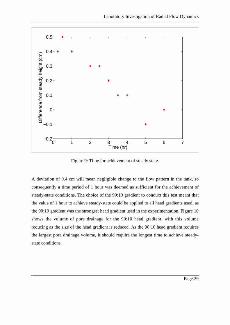
Assuming that steady height was achieved after six hours, the results show that there is
only a change in height of 0.4 cm between the reading after 1 hour and the steady height
(Figure 9).
Laboratory Investigation of Radial Flow Dynamics
Page 29
0 1 2 3 4 5 6 7−0.2
−0.1
0
0.1
0.2
0.3
0.4
0.5
Time (hr)
Diff
eren
ce fr
om s
tead
y he
ight
(cm
)
Figure 9: Time for achievement of steady state.
A deviation of 0.4 cm will mean negligible change to the flow pattern in the tank, so
consequently a time period of 1 hour was deemed as sufficient for the achievement of
steady-state conditions. The choice of the 90:10 gradient to conduct this test meant that
the value of 1 hour to achieve steady-state could be applied to all head gradients used, as
the 90:10 gradient was the strongest head gradient used in the experimentation. Figure 10
shows the volume of pore drainage for the 90:10 head gradient, with this volume
reducing as the size of the head gradient is reduced. As the 90:10 head gradient requires
the largest pore drainage volume, it should require the longest time to achieve steady-
state conditions.

Laboratory Investigation of Radial Flow Dynamics
Page 30
R coordinate
Ele
vati
on
Downstream water level
Upstream water level
Phreatic surface
Volume of pore drainage required
Figure 10: Pore drainage areas for different head gradients
3.3.2 Flow
Total flow through the tank was measured by collecting the flow at the downstream end
of the flow tank. The time taken for this flow to fill a 1 L container was measured in
order to calculate a flow rate for the system. This process was then replicated twice with
an average value used as a measure for flow rate. Total flow was measured for six head
differentials: 90:10, 90:20, 90:40, 90:60, 90:70 and 90:75.
3.3.3 Travel times
Travel times in the tank were measured by tracking the paths of coloured food dye
injected at various intervals. The dye was injected using a thin piece of metal pipe
(Diameter ~ 1 mm) that was attached to a 10 mL syringe. Once steady state conditions

Laboratory Investigation of Radial Flow Dynamics
Page 31
were achieved the syringe was pushed slowly through the sand layer along the sidewall of
the tank, 5cm from the upstream end. Once the appropriate height of release was reached
a very small portion of dye was injected (~0.1 mL) and the stopwatch was started. The
dye was then tracked through the grid on the side of the tank. As the dye cloud moved
through the tank it was observed to undergo spreading. The small initial dye cloud
injection into the tank increased in size considerably as it moved through the sand.
To highlight differences in travel times with height a 90:10 head differential was set up
and dye was injected at heights of 80cm, 50cm and 20cm at the upstream end of the tank.
Photos of the tank were then taken at five-minute intervals, until the dye exited the tank.
The choice of a strong hydraulic gradient (90:10) produced large differences in travel
time with height of release, which could be easily identified through the photographs.
Measurements were then made of the time necessary for the front, centre and the tail of
the plume to cross positions 40cm, 70cm and 105cm from the upstream end of the tank
(Figure 6). The centre of the plume provided the best measure of travel time as this
allows spreading effects to be ignored (Figure 11).

Laboratory Investigation of Radial Flow Dynamics
Page 32
Front
Centre
Tail
Figure 11: Dye traveling through radial tank
Travel times were measured from five different release heights: 90, 75, 60, 45 and 15cm.
This was repeated for four head differentials 90:20, 90:40, 90:60 and 90:70. These head
differentials were chosen as they provided a series ranging from large hydraulic gradients
(90:20) to smaller hydraulic gradients (90:70).
3.3.4 Downstream velocity profile
For the 90:10 and 90:75 head differentials downstream travel times were taken. This
involved injecting dye 95 cm from the upstream end and measuring the time to move
5cm downstream. These travel times (t) were measured at 5 cm height intervals from a
height of 90 cm to a height of 10 cm and were then converted to horizontal velocities via:

Laboratory Investigation of Radial Flow Dynamics
Page 33
tcmVelocity
5sec)/( =
(7)
The 90:10 head differential was chosen as it results in the formation of a large seepage
face, thus allowing for the observation of a broad velocity profile above the downstream
well height. The 90:75 head differential was also studied in conjunction; although it only
results in the formation of a small seepage face, it does enable observation of flow
velocities over a broad range below the downstream well height. The 90:10 head
differential does not allow this observation. The flow velocities measured here are not
true downstream flow velocities, as the design of the model restricts observation of dye
any closer to the downstream end of the tank. The observations however are close to the
general profile observed at the downstream end.
3.3.5 Streamlines
Streamlines from the tank were measured simultaneously with the travel times. As the
injected dye plume was observed to move through the tank the height of the plume centre
was marked at 5cm intervals along the tank, corresponding to the vertical lines of the grid
on the tank. This was repeated for the same head differentials as described in Section
3.3.3, at release heights of 90, 75, 60, 45, 30 and 15 cm.
A set of streamlines was also produced for the 90:10 head differential. For these
streamlines dye was regularly injected at the same height. This allowed for the formation
of a complete streamline moving from the upstream to the downstream end of the tank.
Photographs were taken of streamlines observed at 5cm intervals from a height of 10cm
to a height of 90cm. The 90:10 head differential was chosen to observe these streamlines
as it involves an extreme hydraulic gradient being applied to the tank. This extreme
hydraulic gradient results in large vertical flows and hence the greatest shift from the
Dupuit-Forchheimer model.
Laboratory Investigation of Radial Flow Dynamics
Page 34
3.3.6 Potentiometric levels
To measure potentiometric levels fluid height in each of the piezometers was noted for
the four head differentials described in Section 3.3.3. For piezometers located in the
unsaturated zone no fluid levels were observed.
3.4 Numerical models
3.4.1 Variably-saturated flow equation
The numerical model developed by Clement (1993), and described in Appendix B, was
used to solve the variably-saturated flow equation. Parameters required by the model
include the saturated hydraulic conductivity of the porous medium Ks, the Van
Genuchten parameters αv and nv and the saturated (θs) and residual (θr) water contents.
The Van Genuchten parameters are used to describe the soil properties, with αv providing
a measure of the first moment of the pore size density function [L-1] and nv an inverse
measure of the second moment of the pore size density function (Wise, 1991; Wise et al.,
1994).
The 120 cm × 95 cm domain was discretised using a 39 node × 39 node grid. The
following parameters were used in the model: Ks = 48 m/day, θs = 0.3, θr = 0, α v = 2.0
and nv = 2.0. The value for Ks was calculated using a constant head permeameter. This
value was then validated using a fixed head permeameter. The other soil parameters θs,
θr, αv and nv were not calculated but instead typical values were taken. The effects of soil
parameters θs, θ r, α v and nv are not of particular concern as both Shamsai and
Naraisimhan (1991) and Clement et al. (1996) have shown that their effects are negligible
for radial flow systems.
Laboratory Investigation of Radial Flow Dynamics
Page 35
The variably-saturated flow model enables prediction of the pressure heads, flow
velocities and the position of the phreatic surface for the radial flow system. The model
also calculates the flow into the system at the upstream end and the flow out of the
system at the downstream end. These two values are expected to be close for mass
balance, however some error occurs. As a result, the flow rate of the system is measured
by taking an average of the inlet and outlet values. The output from the variably-saturated
model was used in conjunction with a particle tracking model, as shown in Simpson and
Clement (2001), to predict travel times and streamlines.
3.4.2 Dupuit-Forchheimer flow equation: Evaluation of travel times
Based on Dupuit-Forchheimer theory, application of equations (2) and (3) directly
computes total flow and head distributions. To calculate the total travel time using the
Dupuit-Forchheimer model, equation (3) was differentiated with respect to radius and
then Darcy’s Law was applied:
( )( ) ( ) ( )
( )
d
t
os
s
ssr
WR
WWRW
WRW
WR
tdtrf
drKn
dtrf
drKn
rfn
K
dr
dh
n
K
dt
drv
rfrr
rrhhh
rrrr
hh
dr
dh
d
==
=
===
=??−+
−=
−
10
110
2/1
22222
)(
)(
)(
)(/ln
/ln(
/ln2
(8)
The integral on the left-hand side of the equation was evaluated numerically using the
trapezoidal method.

Laboratory Investigation of Radial Flow Dynamics
Page 36
4.0 Analysis and Synthesis
4.1 Saturated Sand Hydraulic Conductivity
The method for calculating the value for saturated hydraulic conductivity is included in
Appendix C. The test measured a saturated hydraulic conductivity of 48 m/day for the
tightly packed sample and 86 m/day for the unpacked sample of the porous medium.
The falling head test was then used as a method to validate these results. The falling head
test predicted a saturated hydraulic conductivity of 49 m/day for the tightly packed
sample thus supporting the value observed in the constant head test. The procedure used
for the falling head test is also included in Appendix C.
As the packing conditions in the tank itself will lie between the tightly packed and
unpacked conditions we can infer that the saturated hydraulic conductivity of the porous
medium lies between 48 and 86 m/day. A more accurate value is difficult to quantify due
to the difficulties in reproducing the packing conditions in the tank with those in the
constant head permeameter.
4.2 Flow
The total flow rate through the system measured for six head differentials is included
below, together with the values predicted by the Dupuit-Forchheimer and variably-
saturated flow models for the hydraulic gradient of 48 m/day (Table 1).

Laboratory Investigation of Radial Flow Dynamics
Page 37
Table 1: Observed and measured flow rates for various head differentials
4.2.1 Variably-saturated flow
Table 1 includes the flow predicted by the variably-saturated flow model at both the
inflow and outflow faces, together with the percentage difference between the flow at the
inflow and outflow faces. The results reveal a percentage difference of less than 1% for
largest four head gradients, while for the smallest head gradients 90:70 and 90:75 large
errors in flow between the inflow and outflow faces are observed. The relatively coarse
grid (39 nodes × 39 nodes) used to study the problem results in these errors. For smaller
head gradients seepage faces still develop however they are not as large as those for
larger head gradients. For the 90:70 and 90:75 head differentials the variably-saturated
flow model predicted that no seepage faces would be formed which is in fact incorrect, as
some small seepage faces would still form. The seepage face is important when
calculating the flow out of the system and consequently its incorrect estimation explains
the deviation that exists between the flows observed for the inflow and outflow faces.
Figure 3 shows the high outflow velocities predicted along the seepage face. The use of a
finer grid size enables more accurate prediction of the seepage face height, and as a result
more accurate prediction of the flow rate. To highlight the importance of the grid size to
the flow rate, calculation was repeated for two finer grids, 77 nodes × 77 nodes and 153
nodes × 153 nodes at the head differential of 90:75 (Table 2).
Flow (m^3/day) 10 20 40 60 70 75Observed 3.05 2.74 2.56 1.76 1.14 0.76
Dupuit-Forchheimer 2.00 1.93 1.63 1.13 0.80 0.62Variably saturated in 2.12 2.03 1.71 1.17 0.73 0.58
Variably saturated out 2.10 2.02 1.70 1.18 0.86 0.66Variably saturated ave 2.11 2.03 1.71 1.18 0.79 0.62Variably saturated %
difference 0.83 0.58 0.26 0.92 18.51 15.33
Downstream well height (cm), upstream well height = 90cm

Laboratory Investigation of Radial Flow Dynamics
Page 38
Table 2: Flow rate predicted by variably-saturated flow model at different grid sizes for a
90:75 head differential
The results show that refinement of the grid leads to a reduction in the percentage flow
differences between the outflow and inflow faces. The table also shows that the grid
refinement leads to a convergence onto a flow value, with the average value of flow from
the inflow and outflow faces remaining relatively consistent for all three grids. As a
consequence, the use of the average flow from the 39 node × 39 node grid was deemed as
an appropriate measure of flow for the variably-saturated flow model.
4.2.2 Analysis of physical results
The flow observed in the model, together with flow predicted by the Dupuit-Forchheimer
and variably saturated flow models for a hydraulic conductivity of 48 m/day is included
in Figure 12.
Flow (m^3/day) 39*39 77*77 153*153Variably saturated in 0.58 0.59 0.60
Variably saturated out 0.66 0.65 0.64Variably saturated ave 0.62 0.62 0.62Variably saturated %
difference 15.33 8.87 6.56
Number of nodes

Laboratory Investigation of Radial Flow Dynamics
Page 39
0 10 20 30 40 50 60 70 800
0.5
1
1.5
2
2.5
3
3.5
Downstream water level (cm)
Flo
w (
m3 /d
ay)
Observed Dupuit−ForchheimerVariably Saturated
Figure 12: Flow observed at different head differentials with hydraulic conductivity of 48
m/day (upstream head = 90cm)
The results from the three methods of calculating the flow all show a very similar pattern,
with a reduction in the amount of flow with an increase in downstream water level. As
expected a factor exists which separates the values predicted by the variably-saturated
and Dupuit-Forchheimer flow models from those observed in the tank. This factor can be
directly related to the hydraulic conductivity used in the numerical model as the value
used was only an estimate. As flow is directly proportional to hydraulic conductivity the
factor of difference between the observed flow values and the predicted values can be
used to gain an improved estimate of hydraulic conductivity of the porous medium used
in the tank. The factor of difference was calculated between observed flow and the flow
predicted by the variably saturated flow model, as the variably saturated flow model

Laboratory Investigation of Radial Flow Dynamics
Page 40
provides the most accurate prediction of total flow. The calculated factor of difference for
each of the head differentials is included in Table 3.
Table 3: Factor of difference between observed flow and predicted flow from the
variably-saturated flow model
As flow is directly proportional to the hydraulic conductivity multiplication of the
average factor by the previous value for hydraulic conductivity (48 m/day) enables the
calculation of an improved estimate for hydraulic conductivity (67 m/day). This value
lies within the range of 48 – 86 m/day predicted by the constant head test thus supporting
its application to the hydraulic conductivity of the tanks porous medium. Substitution of
67m/day for the hydraulic conductivity reveals that the variably-saturated and Dupuit-
Forchheimer models fit the observed flow data well (Figure 13).
Downstream head (cm) 10 20 40 60 70 75
Observed 3.05 2.74 2.56 1.76 1.14 0.76Variably saturated 2.11 2.03 1.71 1.18 0.79 0.62 Average
Factor 1.44 1.35 1.50 1.50 1.44 1.23 1.41

Laboratory Investigation of Radial Flow Dynamics
Page 41
0 10 20 30 40 50 60 70 800
0.5
1
1.5
2
2.5
3
3.5
Downstream water level (cm)
Flo
w (
m3 /d
ay)
Observed Dupuit−ForchheimerVariably Saturated
Figure 13: Flow rate predictions using a saturated hydraulic conductivity of 67m/day.
Using the new value for hydraulic conductivity the percentage deviation of the Dupuit-
Forchheimer and variably-saturated flow models from the observed flow rates was
calculated and is included in Table 4.
Table 4: Percentage errors in flow measurements for Dupuit-Forchheimer and variably-
saturated flow models
% Error 10 20 40 60 70 75 AverageDupuit-Forchheimer 8.37 1.09 11.94 11.33 1.32 12.67 7.79Variably saturated 2.87 3.77 6.89 6.81 2.37 12.59 5.88
Downstream well height (cm), upstream well height = 90cm
Laboratory Investigation of Radial Flow Dynamics
Page 42
The variably-saturated flow model generally provides a better prediction of the actual
flow rate in the system (6% error) than the Dupuit-Forchheimer model (8% error). This is
especially highlighted for the 90:10, 90:40 and 90:60 head differentials where unsaturated
flows are larger due to the larger hydraulic gradients involved. At head differentials
where the Dupuit-Forchheimer model provides a better prediction of the total flow
(90:20, 90:70 and 90:75) the error differences between the variably-saturated and Dupuit-
Forchheimer model predictions are small and can be accounted for as experimental error.
Large errors in prediction of flow by both models for the 90:75 head differential indicate
that the observed value may have been incorrectly measured. Overall the errors between
the two data sets are small and the use of 67m/day for the hydraulic conductivity is
deemed appropriate.
4.3 Travel times
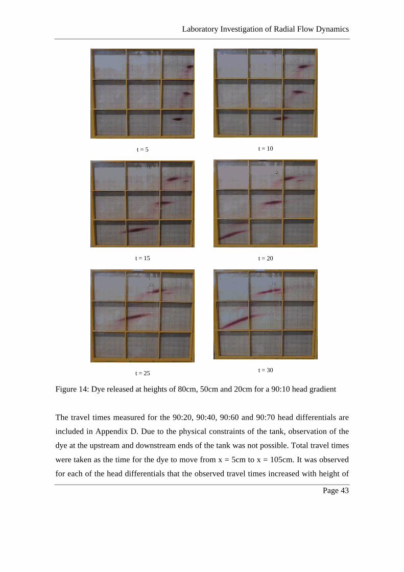
A clear indication of the variation of travel time with height is shown in Figure 14 where
for a 90:10 head differential photos were taken of dye released at heights of 80cm, 50cm
and 20cm at five minute intervals.
Laboratory Investigation of Radial Flow Dynamics
Page 43
Figure 14: Dye released at heights of 80cm, 50cm and 20cm for a 90:10 head gradient
The travel times measured for the 90:20, 90:40, 90:60 and 90:70 head differentials are
included in Appendix D. Due to the physical constraints of the tank, observation of the
dye at the upstream and downstream ends of the tank was not possible. Total travel times
were taken as the time for the dye to move from x = 5cm to x = 105cm. It was observed
for each of the head differentials that the observed travel times increased with height of
t = 5
t = 15
t = 25
t = 10
t = 20
t = 30

Laboratory Investigation of Radial Flow Dynamics
Page 44
release (Figures 15-18). Figures 15-18 also include the travel times predicted by the
Dupuit-Forchheimer model, as well as times predicted by variably-saturated model for a
hydraulic conductivity of 67m/day.
0 20 40 60 80 1000
5
10
15
20
25
30
35
Height of release (cm)
Tra
vel t
ime
(min
)Observed Variably SaturatedDupuit−Forchheimer
Figure 15: Total travel times for 90:20 head differential
0 20 40 60 80 1000
5
10
15
20
25
30
35
40
45
50
Height of release (cm)
Tra
vel t
ime
(min
)
Observed Variably SaturatedDupuit−Forchheimer
Figure 16: Total travel times for 90:40 head differential
Laboratory Investigation of Radial Flow Dynamics
Page 45
0 20 40 60 80 1000
10
20
30
40
50
60
Height of release (cm)
Tra
vel t
ime
(min
)
Observed Variably SaturatedDupuit−Forchheimer
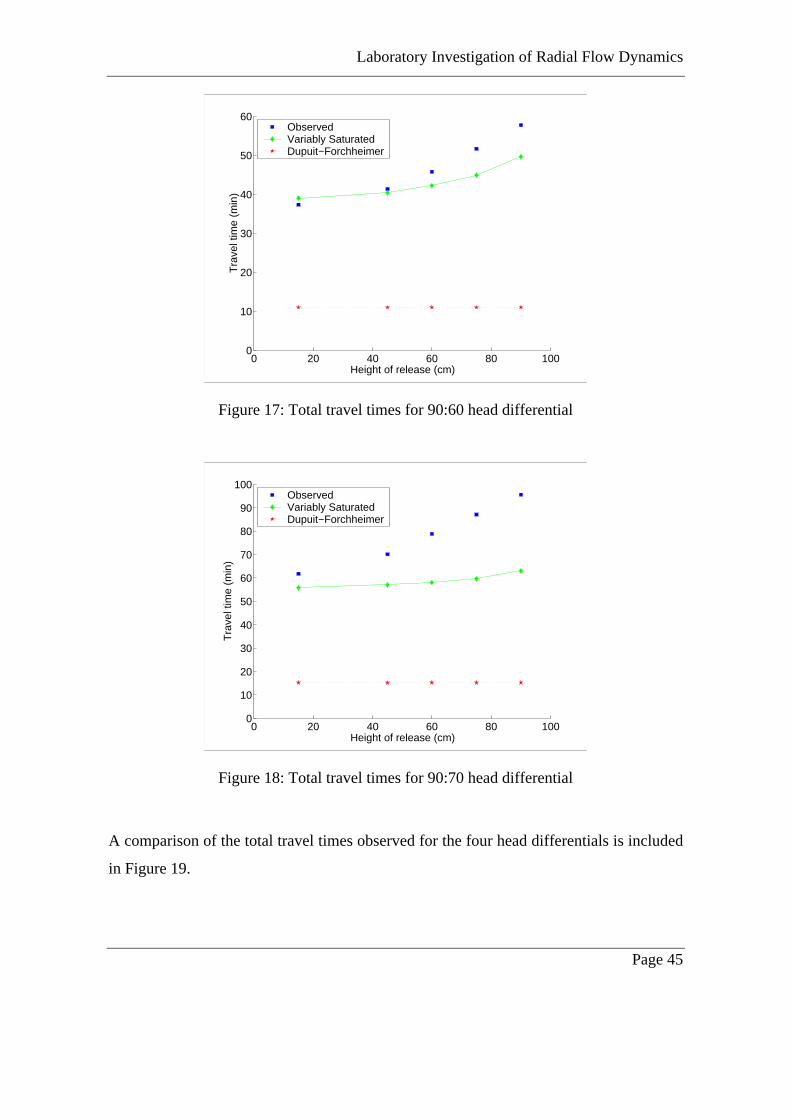
Figure 17: Total travel times for 90:60 head differential
0 20 40 60 80 1000
10
20
30
40
50
60
70
80
90
100
Height of release (cm)
Tra
vel t
ime
(min
)
Observed Variably SaturatedDupuit−Forchheimer
Figure 18: Total travel times for 90:70 head differential
A comparison of the total travel times observed for the four head differentials is included
in Figure 19.

Laboratory Investigation of Radial Flow Dynamics
Page 46
0 20 40 60 80 1000
10
20
30
40
50
60
70
80
90
100
Height of release (cm)
Tra
vel t
ime
(min
)
90:2090:4090:6090:70
Figure 19: Comparison of total travel times for changing head differentials
The reason for the variation of travel time with height is the combination of two factors.
The first being that as height increases so does the length of the travel path to the
downstream end, with a longer path meaning that it takes the dye longer to move to the
downstream end. Longer travel paths with height are due to paths at higher release
heights showing larger curvature, while paths at lower release heights are flatter and
therefore shorter. Secondly, the reduction of pressure with height leads to stronger
hydraulic gradients and thus stronger flow velocities towards the bottom of the tank.
Factorial differences in travel time of dye released at a height of 90cm and dye released at
a height of 15cm range from 1.91 times for a 90:20 head differential to 1.55 for a 90:70
head differential (Figure 20).

Laboratory Investigation of Radial Flow Dynamics
Page 47
0 10 20 30 40 50 60 70 800
0.2
0.4
0.6
0.8
1
1.2
1.4
1.6
1.8
Downstream well height (cm)
Tim
e(90
)/T
ime(
15)
Figure 20: Comparison of total travel times for dye released at 90cm and dye released at
15cm.
These are significant deviations in travel time especially considering that the Dupuit-
Forchheimer model predicts that travel times should not change with height. Figures 15-
18 also show that the Dupuit-Forchheimer model underestimates the total travel time in
all cases studied. Using the Dupuit-Forchheimer model could therefore be very costly in
cases involving contamination transport, as underestimation of the travel time for a radial
pumping situation could result in underestimation of pumping times required to remove
contaminants from the system.
These results also show that as the height of release increases the change in travel time
for a further increase in height of release becomes greater. This is shown by the points
curving upwards as height of release is increased for Figure 19. This result is explained

Laboratory Investigation of Radial Flow Dynamics
Page 48
by the changes in the length of travel paths and changes in the flow velocity for different
heights of release. At lower release heights the differences between the paths at different
release heights are relatively small, explaining why there are only small deviations in
travel time between release heights. At higher points of release the lengths of flow paths
are much more dependent on height of release due to the larger curvature of flow for
these paths, and hence so is travel time. Flow velocities are also seen to generally reduce
as height of release is increased. For higher points of release larger reductions in velocity
are observed for a further increase in release height. This affect adds to the curvature of
the travel time graphs in Figure 19. Flow through the unsaturated zone is also important
in order to describe the variation of travel time with height. This is particularly valid for a
release height of 90cm where the dye crosses the phreatic surface into the unsaturated
zone. Flow through this zone is considerably slower than flow through the saturated zone
so consequently this affect leads to further increases in travel time. This explains further
the curving upwards of the points in Figure 19 for all four head differentials.
Figure 19 also shows that the travel times are all generally seen to reduce as the hydraulic
gradient is increased for all heights of release. This is as would be expected as larger
hydraulic gradients produce larger flow velocities. From Figure 19 it can also be noted
that there is a much smaller difference in travel times between the 90:20 and 90:40 head
differentials than there is between the 90:40 and 90:60 head gradients. Similar can be said
between the 90:40 and 90:60 and the 90:60 and 90:70 head differentials. This shows that
travel times are much more sensitive to changes in head gradient at smaller head
gradients (e.g. 90:70) than for larger head gradients (e.g. 90:20).
Figures 15-18 indicate that the variably-saturated flow equation provides a better fit of
the observed travel times for situations of larger hydraulic gradient (e.g. 90:20, 90:40)
than for smaller hydraulic gradients (e.g. 90:70). It is also noticeable that better
approximations of total travel time are provided for dye released at lower heights. As
height of release is increased the deviation between the variably-saturated model results
and the observed results also increases. Where poor predictions of travel times occur:
small head gradients and high heights of release, the slowest travel times observed. The

Laboratory Investigation of Radial Flow Dynamics
Page 49
slower the travel time the larger the amount of spreading of the dye plume during its path.
Greater spreading makes it more difficult to identify the centre of the plume and
consequently errors in measuring the travel times are larger. Another reason for this
deviation lies in the fact that as the travel time increases so does the number of
heterogeneities encountered dye plume as it moves through the tank. In the variably-
saturated flow model we assume a homogeneous medium, however in reality some small
heterogeneities still exist. For the shorter travel times the affect of heterogeneities is not
as pronounced, however as travel times increase so do the errors from the variably-
saturated flow model. The largest errors in the prediction of dye travel times occur for
dye released at a height of 90cm. This height corresponds to the top of the water table at
the upstream end, where the length of the travel path is at a maximum and where flow
moves through unsaturated zone. The longer travel paths and the slowing of flow in the
unsaturated zone results in higher travel times for dye released at this height, making
prediction of travel times difficult. This explains the failure of the variably-saturated flow
model to accurately predict travel times at this height of release. Omitting the results
from the 90:70 head differential where some experimental errors occur, the results show
that the variably-saturated model provides a reasonable prediction of total travel time for
the radial flow system with an average error of 8% (Table 5).
Table 5: Comparison of errors in travel times predicted by the variably-saturated flow
model and those physically observed.
Height (cm) 20 40 60 Average
90 9.78 13.68 16.33 13.2675 3.14 4.95 15.04 7.7160 7.55 1.56 8.42 5.8445 9.86 2.25 2.34 4.8215 15.70 4.83 4.21 8.25
Average 9.21 5.45 9.27 7.98
% Error
Laboratory Investigation of Radial Flow Dynamics
Page 50
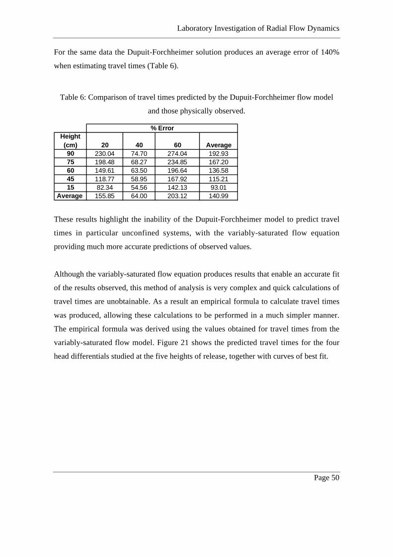
For the same data the Dupuit-Forchheimer solution produces an average error of 140%
when estimating travel times (Table 6).
Table 6: Comparison of travel times predicted by the Dupuit-Forchheimer flow model
and those physically observed.
These results highlight the inability of the Dupuit-Forchheimer model to predict travel
times in particular unconfined systems, with the variably-saturated flow equation
providing much more accurate predictions of observed values.
Although the variably-saturated flow equation produces results that enable an accurate fit
of the results observed, this method of analysis is very complex and quick calculations of
travel times are unobtainable. As a result an empirical formula to calculate travel times
was produced, allowing these calculations to be performed in a much simpler manner.
The empirical formula was derived using the values obtained for travel times from the
variably-saturated flow model. Figure 21 shows the predicted travel times for the four
head differentials studied at the five heights of release, together with curves of best fit.
Height (cm) 20 40 60 Average90 230.04 74.70 274.04 192.9375 198.48 68.27 234.85 167.2060 149.61 63.50 196.64 136.5845 118.77 58.95 167.92 115.2115 82.34 54.56 142.13 93.01
Average 155.85 64.00 203.12 140.99
% Error

Laboratory Investigation of Radial Flow Dynamics
Page 51
Figure 21: Predicted travel times for four head differentials together with their quadratic
curves of best fit
A second-degree polynomial (quadratic) fit was used. This revealed an almost perfect fit
for all four head differentials (R2~1 in all cases). Considering the general equation for a
quadratic of y=Ax2+Bx+C we observed that the value for A is the same for the 90:20,
90:40 and 90:60 head differentials. The value for the 90:70 head differential was
observed to be slightly different so as a consequence this data was neglected when
finding the empirical formula. The values for B for the 90:20, 90:40 and 90:60 head
differentials showed a general reduction in the value of B with downstream well height.
The values of B were plotted against the downstream well heights and a linear curve was
fitted, giving the relation: B = -0.0007H - 0.0589 where H is the downstream well height
and R2 = 0.9633. The C values were observed to increase as H was increased, with a plot
of C against H producing the linear relationship: C = 0.488H + 9.3673 with R2 = 0.9375.
Substitution of the expressions for B and C into the general expression produced the
y = 0.0015x2 - 0.0633x + 56.609
R2 = 0.9886
y = 0.0023x2 - 0.1008x + 40.101
R2 = 0.9963
y = 0.0024x2 - 0.0912x + 25.976
R2 = 0.9983
y = 0.0024x2 - 0.0718x + 20.582
R2 = 0.9988
0
10
20
30
40
50
60
70
0 10 20 30 40 50 60 70 80 90 100
Distance from downstream end (cm)
Tra
vel t
ime
(min
)
Head Differential 90:20 Head Differential 90:40 Head Differential 90:60Head Differential 90:70 Poly. (Head Differential 90:70) Poly. (Head Differential 90:60)Poly. (Head Differential 90:40) Poly. (Head Differential 90:20)
Laboratory Investigation of Radial Flow Dynamics
Page 52
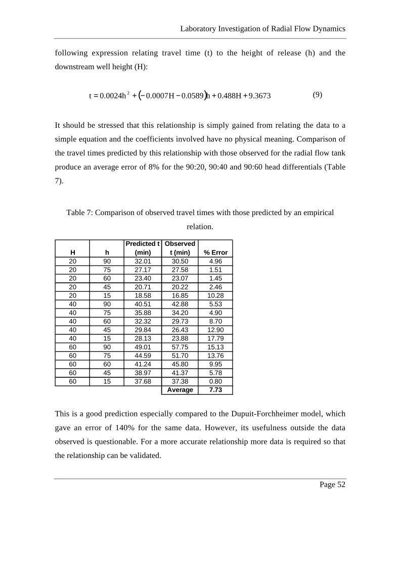
following expression relating travel time (t) to the height of release (h) and the
downstream well height (H):
( ) 3673.9H488.0h0589.0H0007.0h0024.0t 2 ++−−+= (9)
It should be stressed that this relationship is simply gained from relating the data to a
simple equation and the coefficients involved have no physical meaning. Comparison of
the travel times predicted by this relationship with those observed for the radial flow tank
produce an average error of 8% for the 90:20, 90:40 and 90:60 head differentials (Table
7).
Table 7: Comparison of observed travel times with those predicted by an empirical
relation.
This is a good prediction especially compared to the Dupuit-Forchheimer model, which
gave an error of 140% for the same data. However, its usefulness outside the data
observed is questionable. For a more accurate relationship more data is required so that
the relationship can be validated.
H hPredicted t
(min)Observed
t (min) % Error20 90 32.01 30.50 4.9620 75 27.17 27.58 1.5120 60 23.40 23.07 1.4520 45 20.71 20.22 2.4620 15 18.58 16.85 10.2840 90 40.51 42.88 5.5340 75 35.88 34.20 4.9040 60 32.32 29.73 8.7040 45 29.84 26.43 12.9040 15 28.13 23.88 17.7960 90 49.01 57.75 15.1360 75 44.59 51.70 13.7660 60 41.24 45.80 9.9560 45 38.97 41.37 5.7860 15 37.68 37.38 0.80
Average 7.73

Laboratory Investigation of Radial Flow Dynamics
Page 53
For each of the head differentials the time for the centre of the dye plume to reach certain
points in the tank is shown below (Figures 22-25).
0 20 40 60 80 100 1200
5
10
15
20
25
30
35
Distance from upstream end (cm)
Tim
e (m
in)
H=90cmH=75cmH=60cmH=45cmH=15cm
Figure 22: Dye travel times for 90:20 head differential through tank at different heights of
release

Laboratory Investigation of Radial Flow Dynamics
Page 54
0 20 40 60 80 100 1200
5
10
15
20
25
30
35
40
45
Distance from upstream end (cm)
Tim
e (m
in)
H=90cmH=75cmH=60cmH=45cmH=15cm
Figure 23: Dye travel times for 90:40 head differential through tank at different heights of
release

Laboratory Investigation of Radial Flow Dynamics
Page 55
0 20 40 60 80 100 1200
10
20
30
40
50
60
Distance from upstream end (cm)
Tim
e (m
in)
H=90cmH=75cmH=60cmH=45cmH=15cm
Figure 24: Dye travel times for 90:60 head differential through tank at different heights of
release
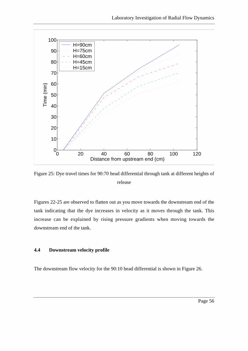
Laboratory Investigation of Radial Flow Dynamics
Page 56
0 20 40 60 80 100 1200
10
20
30
40
50
60
70
80
90
100
Distance from upstream end (cm)
Tim
e (m
in)
H=90cmH=75cmH=60cmH=45cmH=15cm
Figure 25: Dye travel times for 90:70 head differential through tank at different heights of
release
Figures 22-25 are observed to flatten out as you move towards the downstream end of the
tank indicating that the dye increases in velocity as it moves through the tank. This
increase can be explained by rising pressure gradients when moving towards the
downstream end of the tank.
4.4 Downstream velocity profile
The downstream flow velocity for the 90:10 head differential is shown in Figure 26.
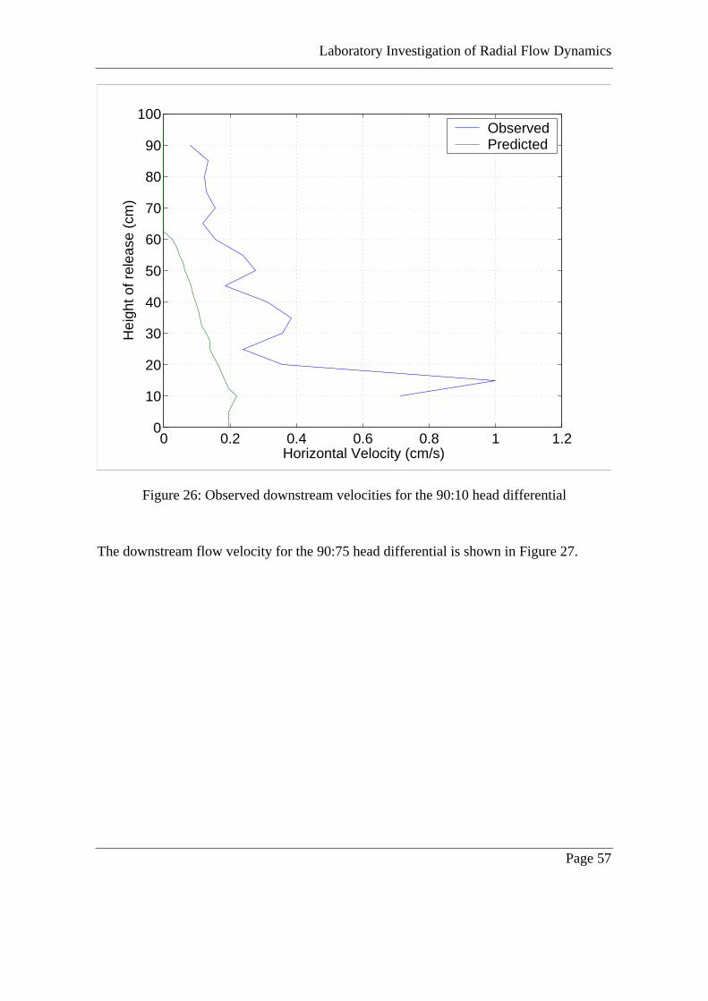
Laboratory Investigation of Radial Flow Dynamics
Page 57
0 0.2 0.4 0.6 0.8 1 1.20
10
20
30
40
50
60
70
80
90
100
Horizontal Velocity (cm/s)
Hei
ght o
f rel
ease
(cm
)Observed Predicted
Figure 26: Observed downstream velocities for the 90:10 head differential
The downstream flow velocity for the 90:75 head differential is shown in Figure 27.

Laboratory Investigation of Radial Flow Dynamics
Page 58
0 0.01 0.02 0.03 0.04 0.05 0.060
10
20
30
40
50
60
70
80
90
100
Horizontal Velocity (cm/s)
Hei
ght o
f rel
ease
(cm
)Observed Predicted
Figure 27: Observed downstream velocities for the 90:75 head differential
For the 90:10 head differential the observed downstream velocities are seen to generally
increase in magnitude in moving towards the downstream well height (Figure 26).
Although the observed values were greater than the predicted values for all heights this
was due to the observed values being measured close to, but not at, the downstream well
height. The observed outflow velocities are seen to peak just above the downstream well
height, rather than at the downstream well height, which was the numerical models
prediction. This difference can once again be explained by the position where flow
velocities were measured. The profile however does fit the general profile expected by
the numerical model, with outflow velocity increasing with decreasing height until close
to the downstream well height. Observations of flow velocities below the downstream
well height were not possible at this head differential due to the tank design.

Laboratory Investigation of Radial Flow Dynamics
Page 59
The 90:75 head differential also shows a profile supporting the numerical data with the
outflow velocity increasing with depth, reaching a peak close to the downstream well
height and then reducing to a steady value below the downstream well height (Figure 27).
Although the velocities observed did not accurately imitate the numerically predicted
profile they do follow the general profile predicted by the numerical model. As for the
90:10 head differential the observed values were larger than the predicted values for all
observation heights. The variably-saturated flow model predicted that the outflow
velocity would reach a steady value much closer to the downstream water level (~50cm)
than the observed values, which stabilise at a lower point (~30cm). As for the 90:10 head
differential measurement of dye velocities close to, but not exactly at the downstream end
of the tank can explain these differences.
These observations highlight the first case where the theoretical downstream flow
velocity profile observed in Figure 3, has been observed physically in a radial system.
This is despite there being difficulties in accurately measuring the downstream flow
velocities, due to both the tank design and errors resulting from the use of dyes to
measure such small flow velocities. Vachaud and Vauclin (1975) had previously
observed this profile in a physical cartesian system, where a similar profile to the radial
system was expected. However, these observations were made from application of
Darcy’s Law to pressure heads observed in piezometers attached to the tank, rather than
by actually observing flow velocities using dye.
These results have particular relevance for contaminant transport as they show that
contamination closer to the downstream height of the well is likely to enter the well faster
than at other heights. As a consequence pump and treat schemes should be designed such
that the level in the pumping well be located as close to the centre of the contaminant
plume as possible, where inflow velocities into the well are maximum. Figure 28 shows a
correct pump and treat design, with the extraction well height at the same height as the
centre of the contaminant plume. At this height the maximum flow velocity into the well
occurs, allowing for the most efficient extraction of the contaminant.

Laboratory Investigation of Radial Flow Dynamics
Page 60
Figure 28: Correct pump and treat design
4.5 Streamlines
Streamlines observed for the 90:20, 90:40, 90:60 and 90:70 head differentials are
included below, together with the values predicted by the variably-saturated flow model
(Figures 29-32). The data for the streamlines is included in Appendix D.
Flow velocity profile
Extraction well water
level
Contaminant
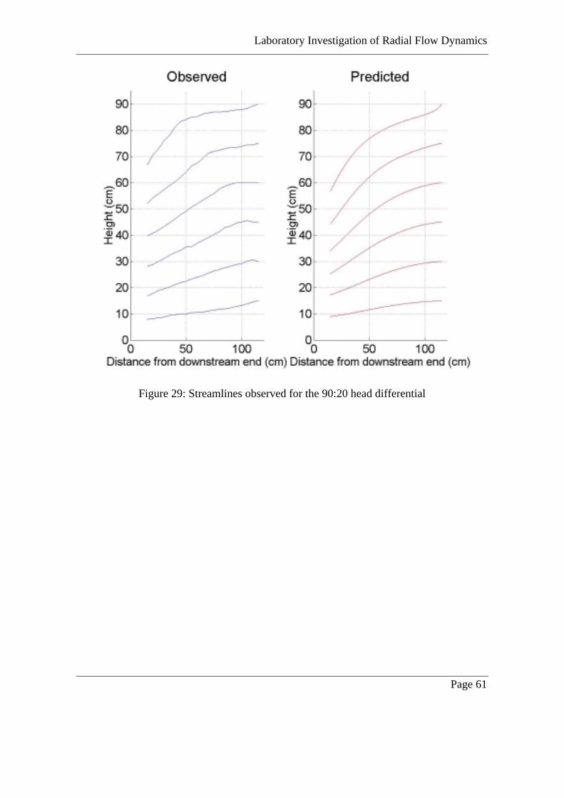
Laboratory Investigation of Radial Flow Dynamics
Page 61
Figure 29: Streamlines observed for the 90:20 head differential

Laboratory Investigation of Radial Flow Dynamics
Page 62
Figure 30: Streamlines observed for the 90:40 head differential

Laboratory Investigation of Radial Flow Dynamics
Page 63
Figure 31: Streamlines observed for the 90:60 head differential

Laboratory Investigation of Radial Flow Dynamics
Page 64
Figure 32: Streamlines observed for 90:70 head differential.
Photographs of streamlines observed for the 90:10 head differential are included below
(Figure 33).

Laboratory Investigation of Radial Flow Dynamics
Page 65
Figure 33: Streamlines observed for a 90:10 head differential
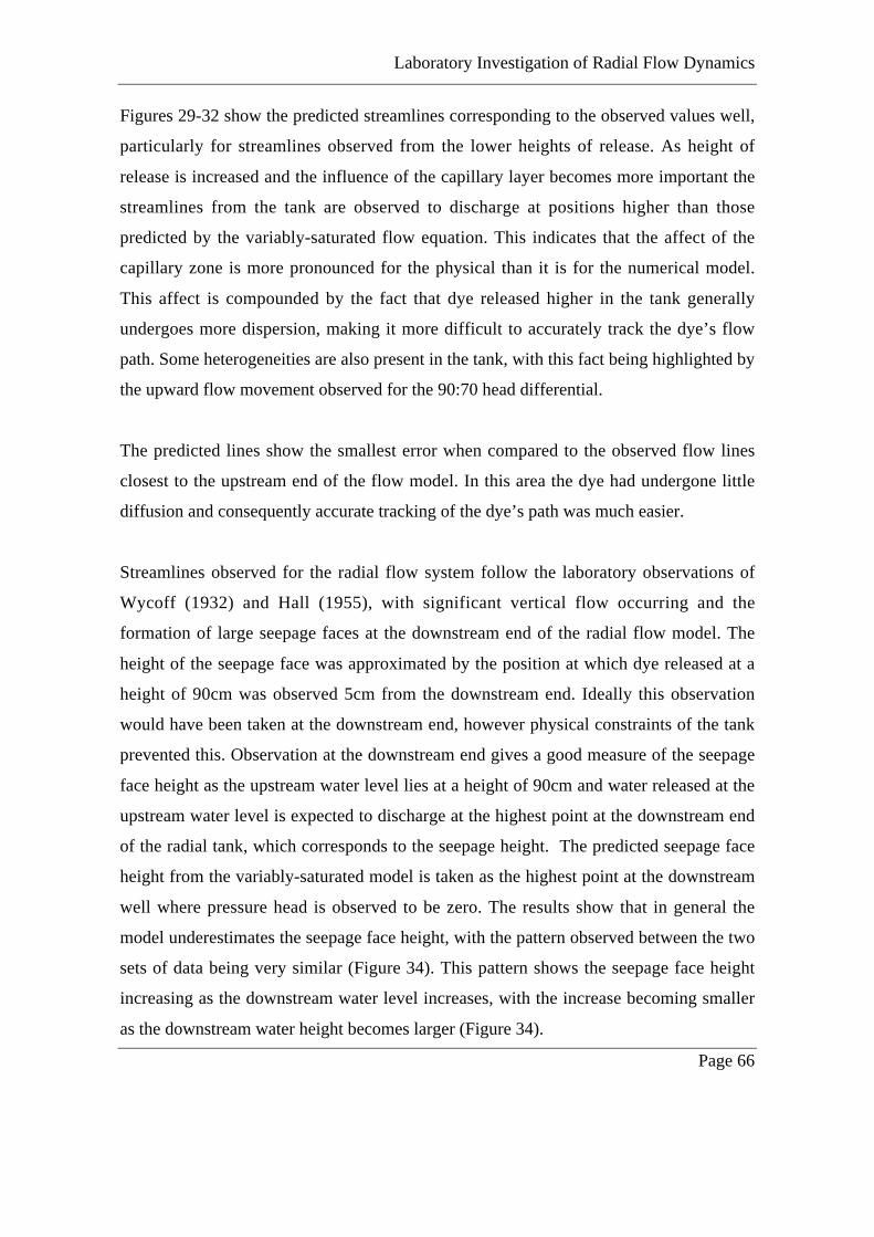
Laboratory Investigation of Radial Flow Dynamics
Page 66
Figures 29-32 show the predicted streamlines corresponding to the observed values well,
particularly for streamlines observed from the lower heights of release. As height of
release is increased and the influence of the capillary layer becomes more important the
streamlines from the tank are observed to discharge at positions higher than those
predicted by the variably-saturated flow equation. This indicates that the affect of the
capillary zone is more pronounced for the physical than it is for the numerical model.
This affect is compounded by the fact that dye released higher in the tank generally
undergoes more dispersion, making it more difficult to accurately track the dye’s flow
path. Some heterogeneities are also present in the tank, with this fact being highlighted by
the upward flow movement observed for the 90:70 head differential.
The predicted lines show the smallest error when compared to the observed flow lines
closest to the upstream end of the flow model. In this area the dye had undergone little
diffusion and consequently accurate tracking of the dye’s path was much easier.
Streamlines observed for the radial flow system follow the laboratory observations of
Wycoff (1932) and Hall (1955), with significant vertical flow occurring and the
formation of large seepage faces at the downstream end of the radial flow model. The
height of the seepage face was approximated by the position at which dye released at a
height of 90cm was observed 5cm from the downstream end. Ideally this observation
would have been taken at the downstream end, however physical constraints of the tank
prevented this. Observation at the downstream end gives a good measure of the seepage
face height as the upstream water level lies at a height of 90cm and water released at the
upstream water level is expected to discharge at the highest point at the downstream end
of the radial tank, which corresponds to the seepage height. The predicted seepage face
height from the variably-saturated model is taken as the highest point at the downstream
well where pressure head is observed to be zero. The results show that in general the
model underestimates the seepage face height, with the pattern observed between the two
sets of data being very similar (Figure 34). This pattern shows the seepage face height
increasing as the downstream water level increases, with the increase becoming smaller
as the downstream water height becomes larger (Figure 34).
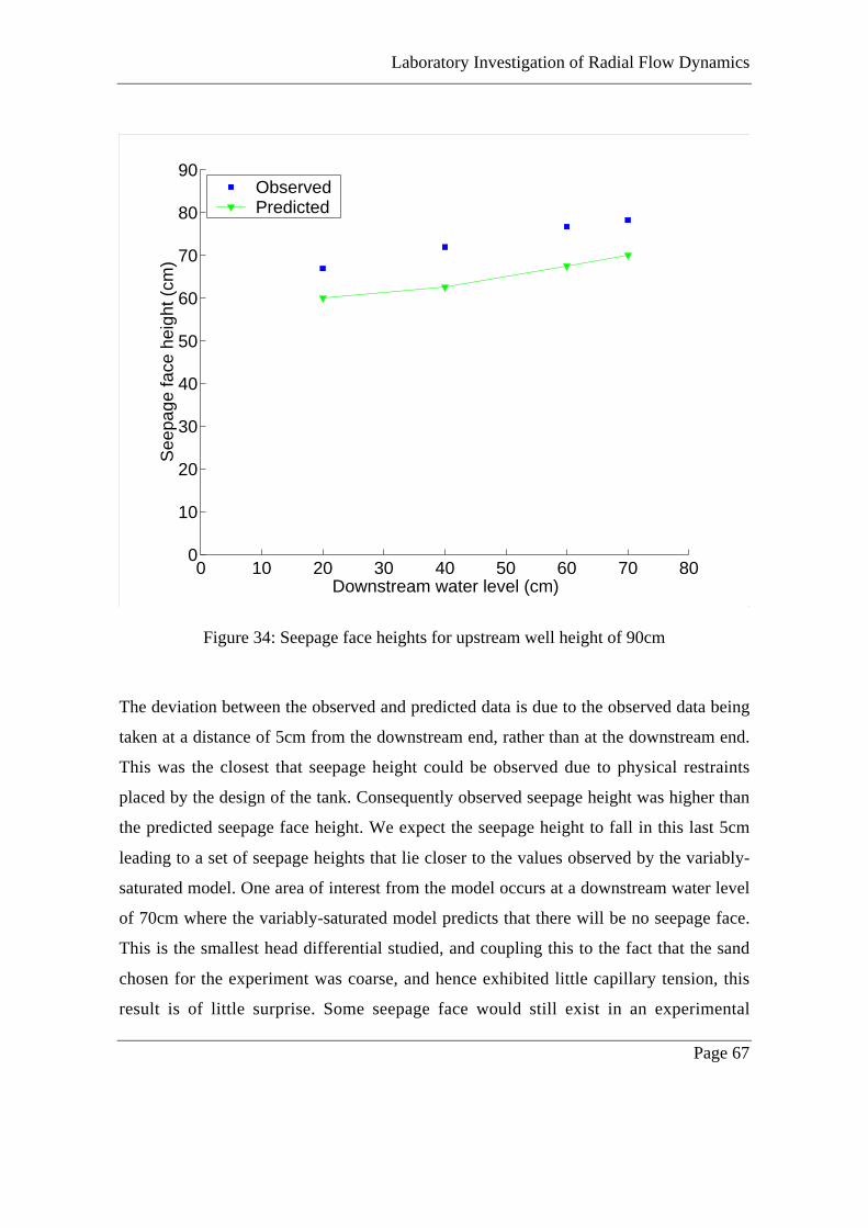
Laboratory Investigation of Radial Flow Dynamics
Page 67
0 10 20 30 40 50 60 70 800
10
20
30
40
50
60
70
80
90
Downstream water level (cm)
See
page
face
hei
ght (
cm)
Observed Predicted
Figure 34: Seepage face heights for upstream well height of 90cm
The deviation between the observed and predicted data is due to the observed data being
taken at a distance of 5cm from the downstream end, rather than at the downstream end.
This was the closest that seepage height could be observed due to physical restraints
placed by the design of the tank. Consequently observed seepage height was higher than
the predicted seepage face height. We expect the seepage height to fall in this last 5cm
leading to a set of seepage heights that lie closer to the values observed by the variably-
saturated model. One area of interest from the model occurs at a downstream water level
of 70cm where the variably-saturated model predicts that there will be no seepage face.
This is the smallest head differential studied, and coupling this to the fact that the sand
chosen for the experiment was coarse, and hence exhibited little capillary tension, this
result is of little surprise. Some seepage face would still exist in an experimental

Laboratory Investigation of Radial Flow Dynamics
Page 68
situation, with the ability of the numerical model to predict this result being limited by
the size of the grid chosen.
4.6 Potentiometric Levels
The potentiometric levels in each of the standpipes were measured from the tank and
compared to the values predicted by the variably-saturated model (Figures 35-38). In
Figures 35-38, the stars represent the observed values and the lines the values predicted
by the variably-saturated flow model, while the values for H represent the height in the
tank where these pressures were observed. The data for piezometric levels is included in
Appendix D.

Laboratory Investigation of Radial Flow Dynamics
Page 69
H=70cm
H=15cm
H=30cm
H=50cm
H=0cm
Figure 35: Piezometric levels for the 90:20 head differential

Laboratory Investigation of Radial Flow Dynamics
Page 70
H=50cm
H=15cm
H=30cm
H=0cm
H=70cm
Figure 36: Piezometric levels for the 90:40 head differential
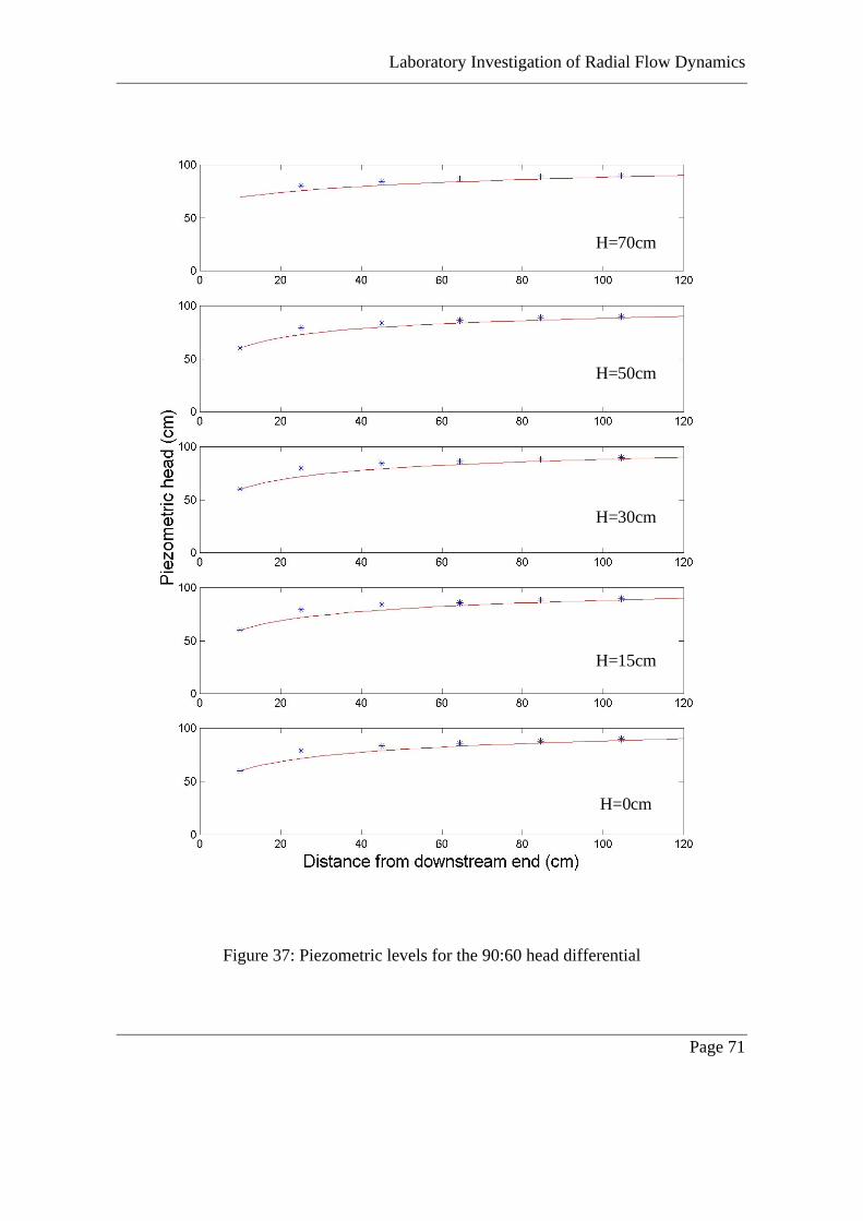
Laboratory Investigation of Radial Flow Dynamics
Page 71
H=0cm
H=15cm
H=30cm
H=50cm
H=70cm
Figure 37: Piezometric levels for the 90:60 head differential

Laboratory Investigation of Radial Flow Dynamics
Page 72
H=70cm
H=50cm
H=30cm
H=15cm
H=0cm
Figure 38: Piezometric levels for the 90:70 head differential

Laboratory Investigation of Radial Flow Dynamics
Page 73
The variably-saturated flow model accurately predicts the piezometric levels for all of the
head differentials observed, with the accuracy of the prediction increasing with reducing
hydraulic gradient. The largest deviations between the observed and predicted values
occurred with the values taken from the piezometers approximately 25cm from the
downstream end at a height of 0cm. In this area the drop in the piezometric head is
largest, with the numerical model predicting lower piezometric heads than those observed
in the tank.
Laboratory Investigation of Radial Flow Dynamics
Page 74
5.0 Conclusions
A detailed understanding of radially driven gravity flow is required to understand well-
flow hydraulics and transfer near pumping wells. Although extensive literature is
available in this area, detailed data on flow velocities and internal flow profiles has been
limited. Using this as a motivation, a number of physical experiments were performed
using a 15o cut of a radial flow system to simulate radial unconfined flow. Using dye
tracers, travel times were measured for four different head differentials, with the results
showing a clear increase in travel time with increasing height of release. This is the first
time where this relationship has been quantitatively observed in a physical system. The
physical results were compared to theoretical values computed from the Dupuit-
Forchheimer and variably-saturated flow models. The Dupuit-Forchheimer flow model
predicts that travel times should not change with height, an assumption that does not
hold. The Dupuit-Forchheimer model was also found to underestimate the travel times
for all heights of release with an average error of 140%. The variably-saturated flow
model however was able to better predict the travel times observed in the physical model,
with an average error of 8%. The increase in travel times with height of release is due to
longer travel paths for increased height of release and reduced flow velocities for
increased height of release.
Observation of travel times from the radial tank also enabled the measurement of
downstream velocity profiles. The velocity profiles for two head differentials revealed an
increase in velocity in moving from the top of the seepage face, with a maximum value
being reached near the downstream water level. Below this level the velocity was seen to
reduce, reaching a steady value below the downstream water level. This is the first case
where the theoretical velocity profile for a radial flow system has been reproduced in a
physical radial model.
Measurements of total flow, streamlines and pressure heads were also taken from the
radial flow model. As expected, comparison of observed total flow with predicted values
from the variably-saturated flow model produced smaller errors (6%) than with the

Laboratory Investigation of Radial Flow Dynamics
Page 75
Dupuit-Forchheimer flow model (8%). This discrepancy is due to unsaturated flow,
which is ignored by the Dupuit-Forchheimer flow model. These errors also show that
despite the Dupuit-Forchheimer providing poor predictions of the travel times, its
predictions for flow are still relatively accurate. The streamlines and pressure heads
observed physically were predicted with good accuracy by the variably-saturated flow
model. The streamlines observed showed significant vertical flow, with the production of
large seepage faces supporting previous work in the area.
These results have particular relevance to the field of contaminant transport where
improved knowledge can help alleviate environmental problems. Application of the
Dupuit-Forchheimer flow model to measure travel times in radial flow systems has been
observed to lead to an underestimation of travel times. In a pump and treat problem this
underestimation could mean underestimation of required pumping periods, with
contaminants remaining in the aquifer after pumping. Application of the variably-
saturated flow model to a pump and treat problem could be much more beneficial.
Applying this model to the highest point of the contaminant plume, where travel times
are generally slowest, should produce an accurate lower bound for the pumping time
required to remove the contaminant plume from the aquifer. It has also been observed
that for most efficient removal of contaminants the well height should be at the same
level as the centre of the contaminant plume. Maximum inflow into the well is observed
at the well height so consequently contaminants at this height will exit the well at the
fastest rate. Application of the concepts discussed here will enable the implementation of
more efficient pumping practices for the removal of contaminants from groundwater
systems.
Laboratory Investigation of Radial Flow Dynamics
Page 76
6.0 Recommendations
During this study an extensive data set was collected from a physical model of radial
flow that included travel times, flow, streamlines and pressure heads. Using this
apparatus there are many areas in which future research could be undertaken.
Further work could enable a reliable empirical relationship for calculating travel times
from height of release and head gradient to be identified. In this study an attempt was
made to derive a similar relationship, however the size of the data set was not large
enough for an effective relationship to be identified. Collection of travel times for
additional hydraulic gradients using the same porous medium would allow for a reliable
relationship to be obtained.
All data collected in this study was for a single porous media. Collection of data over a
number of different porous media would help to gain a greater understanding of the affect
of porous media and unsaturated flow on two-dimensional radial flow systems.
Future studies could also concentrate on measurements made under transient, as well as
steady-state conditions. Performing transient tests, such as a slug test, would enable a
greater understanding of the flow dynamics observed for radial flow systems.

Laboratory Investigation of Radial Flow Dynamics
Page 77
7.0 References
Bear, J., 1979. Hydraulics of Groundwater. McGraw-Hill, New York.
Borelli, M. 1955. Free-surface flow toward partially penetrating wells. Transactions of
the AGU 36: 664-672.
Clement, T.P., 1993. Numerical modeling of variably-saturated seepage face boundaries.
Auburn University, Alabama
Clement, T.P., Wise, W.R. and Molz, F.J., 1994. A physically based, two-dimensional,
finite-difference algorithm for modeling variably-saturated flow. J. Hydrol., 161: 71-90.
Clement, T.P., Wise, W.R., Molz, F.J. and Wen, M., 1996. A comparison of modeling
approaches for steady-state unconfined flow. J. Hydrol., 181: 189-209.
Cooley, R.L., 1983. Some new procedures for numerical solution of variably-saturated
flow problems. Water Resour. Res. 19: 1271-1285.
Dewiest, R.J.M., 1965. History of the Dupuit-Forchheimer Assumptions on Groundwater
Hydraulics. Transactions of the ASAE, Paper 64-717: 508-509
Dupuit, J., 1863. Etudes theoriques et pratiques sur le mouvement des eaux dans les
canaux decouverts et a travers les terrains permeables. (2nd Edition). Dunod, Paris.
Fetter, C.W. 1994. Applied Hydrogeology (Third Edition). Prentice Hall, Upper Saddle
River, New Jersey.
Huyakorn, P.S., Thomas, S.D. and Thompson, B.M., 1984. Techniques for making finite
elements competitive in modeling flow in variably-saturated media. Water Resour. Res.,
20: 1099-1115

Laboratory Investigation of Radial Flow Dynamics
Page 78
Huyakorn, P.S., Springer, E.P., Guvanasen, V. and Wadsworth, T.D., 1986. A three
dimensional finite-element model for simulating water flow in variably-saturated porous
media. Water Resour. Res., 22: 1790-1808.
Mualem, Y., 1976. A new model for predicting hydraulic conductivity of unsaturated
porous media. Water Resour. Res., 12: 513-522
Muskat, M., 1937. The Flow of Homogeneous Fluids through Porous Media. McGraw-
Hill, New York.
Narasimhan, T.N. and Witherspoon, P.A., 1976. An integrated finite difference method
for analyzing fluid flow in porous media, Water Resour. Res., 12(1): 57-64.
Narasimhan, T.N. and Witherspoon, P.A., 1978. An integrated finite difference method
for analyzing fluid flow in deformable porous media, 3, Applications, Water Resour.
Res., 14(6): 1017-1034.
Peterson, D.F., 1957. Hydraulics of wells. Trans. ASCE, 122: 502-517
Pinder, G.F. and Gray, W.G., 1977. Finite Element Simulation in Surface and Subsurface
Hydrology. Academic Press, New York.
Richards, L.A., 1931. Capillary conduction of liquids through porous mediums. Physics,
1: 318:333.
Rubin, J., 1968. Theoretical analysis of two-dimensional, transient flow of water in
unsaturated and partially saturated soils. Soil Sci. Soc. Am. Proc., 32: 607-615.

Laboratory Investigation of Radial Flow Dynamics
Page 79
Shamsai, A. and Narashimhan, T.N., 1991. A numerical investigation of free surface-
seepage face relationship under steady state flow conditions. Water Resour. Res., 27(3):
409-421.
Simpson, M. 2000. Experimental and Numerical Investigation of Unconfined Flow about
a Density Interface. Unpublished thesis proposal. Centre for Water Research, Western
Australia.
Simpson, M.J. and Clement, T.P., 2001. Implications of Dupuit-Forchheimer
approximations on solute transport. Proceedings of the 2nd Australia and New Zealand
GeoEnvironment Conference, Newcastle.
Van Genuchten, M.Th., 1980. A closed-form equation for predicting the hydraulic
conductivity of unsaturated soils. Soil Sci. Soc. Am. J., 44: 892-898.
Vachaud, G. and Vauclin, M., 1975. Comments on ‘A Numerical Model Based on
Coupled One-Dimensional Richards and Boussinesq Equations’ by Mary F. Pikul,
Robert L. Street, and Irwin Remson. Water Resour. Res., 11(3): 506-509.
Wise, W.R., 1991. Discussion of “On the relation between saturated and capillary
retention characteristics”, by S. Mishra and J.C. Parker, September-October 1990 issue,
v. 28, no. 5, pp. 775-777. Ground Water, 29(2): 272-273.
Wise, W.R., Clement, T.P. and Molz, F.J., 1994. Variably-saturated modeling of
transient drainage: sensitivity to soil properties. J. Hydrol., 161: 91-108.
Wycoff, R.D., Botset, H.G. and Muskat, M., 1932. Flow of liquids through porous media
under the action of gravity. Physics, 2: 90-113.
Wycoff, R.D. and Reed, D.W. 1935. Electrical Conduction Models for the Solution of
Water Seepage Problems. Physics, 6: 395-401

Laboratory Investigation of Radial Flow Dynamics
Page 80
APPENDIX A: Numerical Model of two-dimensional, variably-
saturated flow
A two-dimensional finite difference approximation to the variably-saturated flow
equation is used to numerically solve the problem of radial gravity flow. The method of
approximation developed by Clement et al. (1994) is included below:
( )
( )
√√
↵
+−√
√
↵
+
∆+
√√
↵
∆
−√√
↵
+−
√√
↵
∆
−√√
↵
+
∆+
√√↵
∆+∆
−√√
↵
+−
√√↵
∆+∆
−√√
↵
+
∆
≅++
−+
−−
++
−
−
+
+
++
++
−
++
+
++
22
1
2
21
2
2
)()(
2
2
)()(
11
)()()(
1
11
11
11
1
1
1
1
11
11
1
11
1
11
mmmm
mmmm
mmmm
jiij
mm
mm
ijji
mm
mm
ijij
ijijijij
ijijijij
ijijijij
jiij
jiij
ijji
jiij
KKKK
z
z
KK
z
KK
z
rr
rKrK
rr
rKrK
rr
z
K
zK
zrrK
rr
ψψ
ψψ
ψψ
ψψ
ƒθƒ
ƒƒψθ
ƒƒ
ƒƒψθ
ƒƒ (A1)
where Kij is the value of hydraulic conductivity at node ij, ψij is the pressure head at the
node ij and m is the Picard iteration level. The non-linear functions ψ and K(θ) are
linearised using the Picard iteration.
It is possible to rearrange equation (A1) into the form
gedcba mmmmm
ijjiijjiij=++++ +++++
++−−
11111
1111ψψψψψ (A2)
where coefficients a, b, c, d, e and g are defined as

Laboratory Investigation of Radial Flow Dynamics
Page 81
√√↵
∆
+−=
√√↵
∆
+=
√√↵
∆+∆
+√√↵
∆
=
√√↵
∆+∆
+√√↵
∆
=√√↵
∆+
=
+
++
−
+
+
−
−−
z
KKg
z
KKe
rr
KrKr
rrd
rr
KrKr
rrb
z
KKa
mm
mm
ijji
mij
mji
ijij
jiij
mji
mij
ijij
mij
mij
ijij
ijijijji
jiij
2
2,
1
1,
2
1
11
1
21
1
1
1
2
1
and c = -[a + b + d + e]
(A3)
Equation (A2) can be modified to reflect the models boundary conditions leaving a set of
linear equations that can be written in matrix notation as:
bA ˆˆ =ψ (A4)
where
ψ is the vector of unknown pressure heads, ijψ and b is the forcing vector.
Solving equation (A4) yields the unknown pressure heads that can be used to describe the
position of the phreatic surface and flow velocities for the problem.
A.1 Boundary Conditions
Appropriate boundary conditions necessary to solve equation (A4).
Dirichlet nodes
Points where pressure heads are known. These points are represented by ijij ψψ Γ= where
ijψΓ are known pressure heads for nodes ij. For these nodes all coefficients of the matrix
in equation (A2) are zero except c, which is unity. Because of this the known pressure
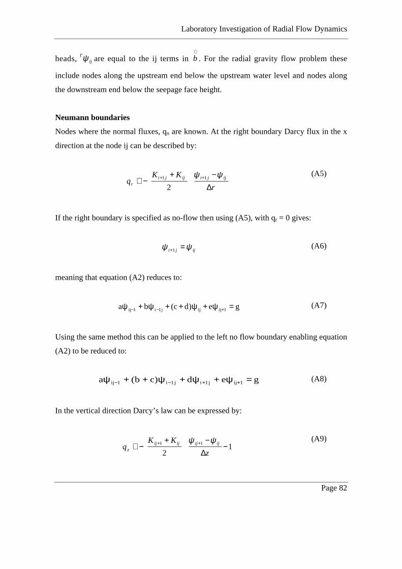
Laboratory Investigation of Radial Flow Dynamics
Page 82
heads, ijψΓ are equal to the ij terms in b . For the radial gravity flow problem these
include nodes along the upstream end below the upstream water level and nodes along
the downstream end below the seepage face height.
Neumann boundaries
Nodes where the normal fluxes, qn are known. At the right boundary Darcy flux in the x
direction at the node ij can be described by:
∆−+
−∪ ++
r
KKq ijjiijji
r
ψψ 11
2
(A5)
If the right boundary is specified as no-flow then using (A5), with qr = 0 gives:
ijji ψψ =+1(A6)
meaning that equation (A2) reduces to:
ge)dc(ba 1ijijj1i1ij =ψ+ψ++ψ+ψ +−−(A7)
Using the same method this can be applied to the left no flow boundary enabling equation
(A2) to be reduced to:
ged)cb(a 1ijj1ij1i1ij =ψ+ψ+ψ++ψ ++−− (A8)
In the vertical direction Darcy’s law can be expressed by:
−∆−+
−∪ ++ 12
11
z
KKq ijijijij
z
ψψ (A9)
Laboratory Investigation of Radial Flow Dynamics
Page 83
Equation (A9) can be used to modify equation (A2) for vertical flux boundary nodes.
The radial gravity flow problem has specified no flux boundaries at the top and the
bottom of the flow domain, and above the upstream water level and seepage face height.
Seepage-face boundaries
Along the seepage face boundaries the nodes are treated as Dirichlet nodes with ψ = 0,
with all nodes above the seepage face specified as areas of no flow (Figure A1).
Figure A1: Pressure levels observed along downstream end of the radial flow problem
The position of the seepage face is initially unknown, with an initial guess of its position
being taken and an iterative process used to determine its actual position. The initial
guess overestimates the position of the seepage, thus ensuring that the node directly
above the seepage face shows a negative ψ value. The process then automatically moves
down one node and recalculates the pressure at the node above the seepage face. This
process is repeated until a positive value for ψ is observed in the node above the seepage
ψ positive
ψ = 0
ψ negative
Seepage face
Downstreamwater level

Laboratory Investigation of Radial Flow Dynamics
Page 84
face. At this time the process is terminated, with the top of the seepage face taken as the
last node where a negative ψ was observed in the node directly above it.
A.2 Soil Properties
The soil properties are described using Van Genuchten’s (1980) closed form of the soil
water retention curve and Mualem’s (1976) unsaturated hydraulic conductivity function.
Pressure head (under tension) and water content are related according to (Van Genuchten,
1980):
Θ =1
1+ (α v ψ nv
? ?
mv
(A10)
where αv, nv and mv = 1-(1/nv) are the Van Genuchten parameters which depend on the
soil properties. αv increases with the first moment and nv increases as the width of the
pore size density function reduces (Wise, 1991; Wise et al., 1994). The parameter Θ is
the effective saturation, described by:
rs
r
θθθθ
−−
=Θ (A11)
where θs describes the saturated water content and θr the residual water content of the soil
under consideration. Using a model produced by Mualem (1976) this water content is
related to hydraulic conductivity (Van Genuchten, 1980):
( ){ }{ } )2/1(2
/111)( ΘΘ−−=Θ vvmm
sKK (A12)
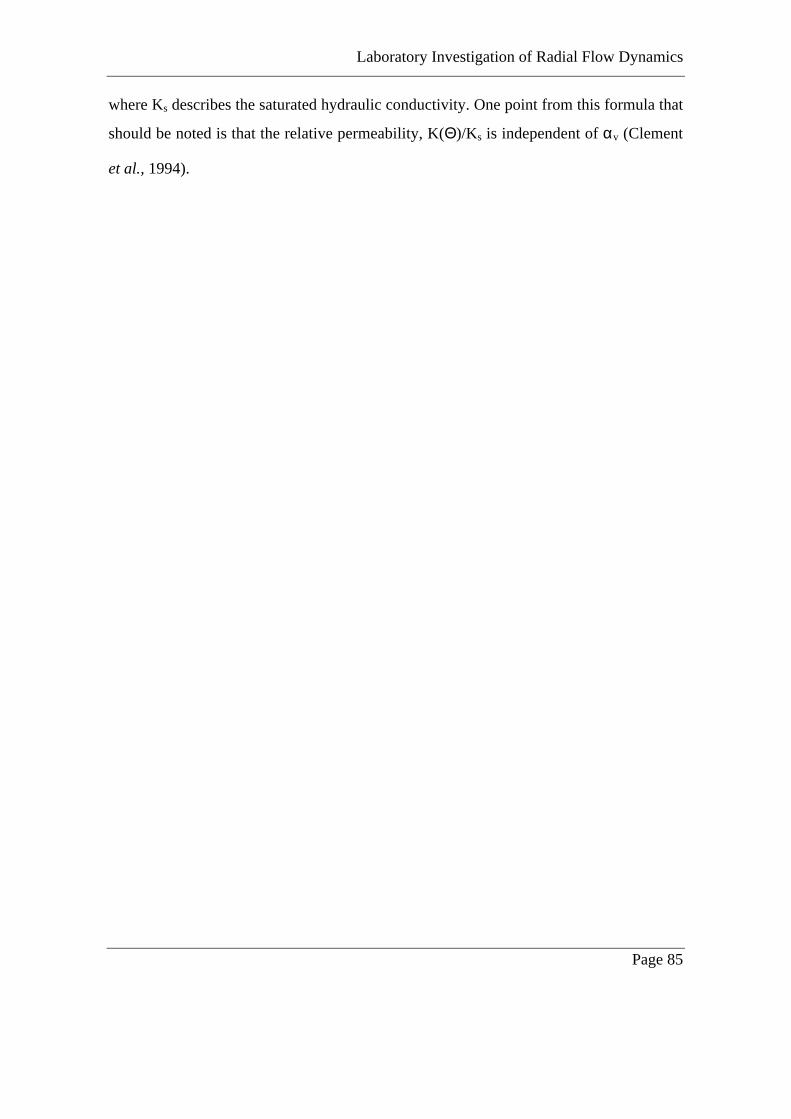
Laboratory Investigation of Radial Flow Dynamics
Page 85
where Ks describes the saturated hydraulic conductivity. One point from this formula that
should be noted is that the relative permeability, K(Θ)/Ks is independent of αv (Clement
et al., 1994).

Laboratory Investigation of Radial Flow Dynamics
Page 86
APPENDIX B: Radial Flow Model Plans
The radial flow tank used was designed by Matthew Simpson for the Centre for Water
Research as part of his PhD (Simpson, 2000). Figures B1, B2 and B3 show the physical
model of the radial flow tank:
Laboratory Investigation of Radial Flow Dynamics
Page 87
Figure B1: Top view of the radial flow tank (Simpson, 2000)

Laboratory Investigation of Radial Flow Dynamics
Page 88
Figure B2: Side view of the radial flow tank.

Laboratory Investigation of Radial Flow Dynamics
Page 89
Figure B3: Piezometers attached to the radial flow tank.

Laboratory Investigation of Radial Flow Dynamics
Page 90
100
33.2
2
10
154.2
0.5
Upstream Screen
Enlargement
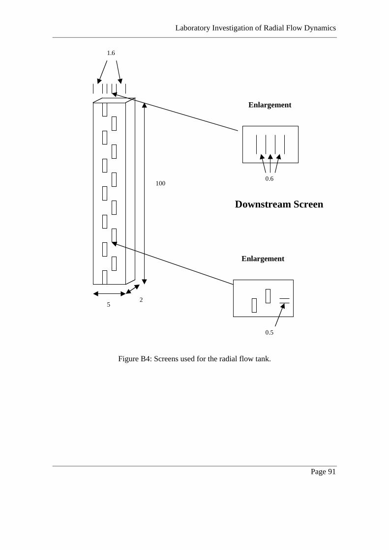
Laboratory Investigation of Radial Flow Dynamics
Page 91
Figure B4: Screens used for the radial flow tank.
100
52
1.6
0.6
Enlargement
Downstream Screen
0.5
Enlargement
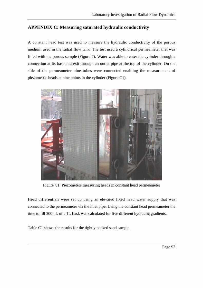
Laboratory Investigation of Radial Flow Dynamics
Page 92
APPENDIX C: Measuring saturated hydraulic conductivity
A constant head test was used to measure the hydraulic conductivity of the porous
medium used in the radial flow tank. The test used a cylindrical permeameter that was
filled with the porous sample (Figure 7). Water was able to enter the cylinder through a
connection at its base and exit through an outlet pipe at the top of the cylinder. On the
side of the permeameter nine tubes were connected enabling the measurement of
piezometric heads at nine points in the cylinder (Figure C1).
Figure C1: Piezometers measuring heads in constant head permeameter
Head differentials were set up using an elevated fixed head water supply that was
connected to the permeameter via the inlet pipe. Using the constant head permeameter the
time to fill 300mL of a 1L flask was calculated for five different hydraulic gradients.
Table C1 shows the results for the tightly packed sand sample.

Laboratory Investigation of Radial Flow Dynamics
Page 93
Table C1: Constant head test results for tightly packed sample
Using the results and equation C1, given by Darcy’s Law, the saturated hydraulic
conductivity was identified as 48 m/day for the tightly packed sample (Fetter, 1994).
Ath
VLK =
(C1)
Table C2 shows the results from the constant head test on an unpacked sand sample.
Table C2: Constant head test results for unpacked sample
The results predict a hydraulic conductivity of 86 m/day for the unpacked sand sample.
Using a different permeameter, the falling head test involved measuring the time for the
water level to drop between two head intervals to measure hydraulic conductivity. The
process was repeated four times, with the results for a tightly packed sand sample
included in Table C3.
500 0.0084541
1 150 300 401 7.48E-07 0.30 25.492 200 300 174 1.72E-06 0.40 44.053 250 300 111 2.70E-06 0.50 55.244 300 300 91 3.30E-06 0.60 56.155 350 300 77 3.90E-06 0.70 56.88
47.56
TestTotal Head
h (mm)
Water Volume V
(mL)
Area A m2
Flow V/t
m3/sec
Time t (s) Total
gradient h/L k (m/day)
Sample Height L (mm)
500 0.0084541
1 150 300 103 2.91E-06 0.30 99.222 200 300 85 3.53E-06 0.40 90.183 250 300 74 4.05E-06 0.50 82.864 300 300 63 4.76E-06 0.60 81.115 350 300 58 5.17E-06 0.70 75.52
85.78
Time t (s) Total
gradient h/L k (m/day)
Flow V/t
m3/sec
Area A m2
TestTotal Head
h (mm)
Water Volume V
(mL)
Sample Height L (mm)
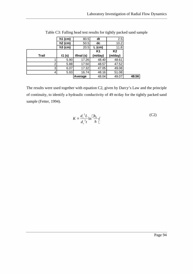
Laboratory Investigation of Radial Flow Dynamics
Page 94
Table C3: Falling head test results for tightly packed sand sample
The results were used together with equation C2, given by Darcy’s Law and the principle
of continuity, to identify a hydraulic conductivity of 49 m/day for the tightly packed sand
sample (Fetter, 1994).
√↵
=h
h
td
LdK
c
t 02
2
ln(C2)
h1 (cm) 80.5 dt 2.5h2 (cm) 50.5 dc 10.2h3 (cm) 20.5 L (cm) 11.8
Trail t1 (s) tfinal (s) K1
(m/day)K2
(m/day)1 5.90 17.26 48.40 48.612 5.88 17.50 48.57 47.523 6.07 17.32 47.05 49.084 5.93 16.74 48.16 51.08
Average 48.04 49.07 48.56

Laboratory Investigation of Radial Flow Dynamics
Page 95
APPENDIX D: Physical results
The travel times for the four head differentials studied are included below (Table D1). In
the table front, centre and tail indicate the front, centre and tail of the plume and x is the
distance from the upstream end of the tank.
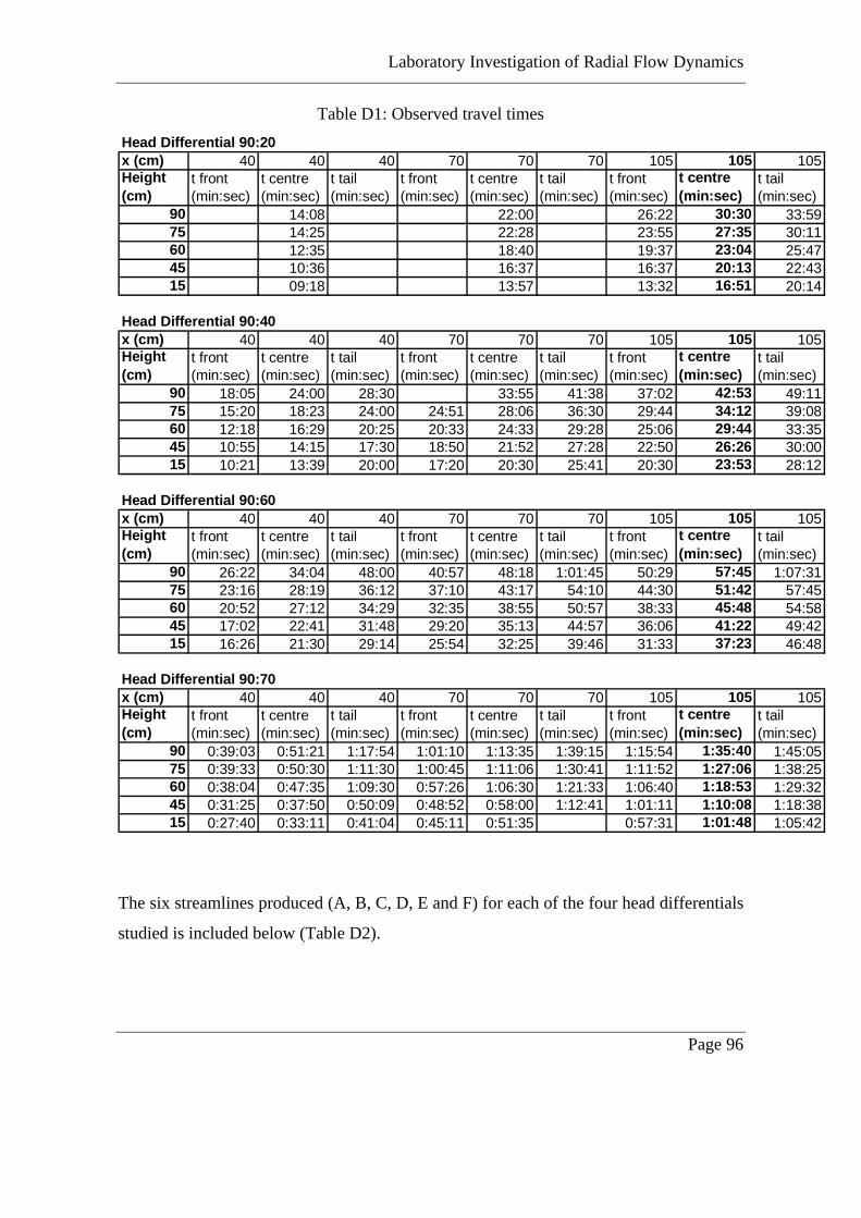
Laboratory Investigation of Radial Flow Dynamics
Page 96
Table D1: Observed travel times
The six streamlines produced (A, B, C, D, E and F) for each of the four head differentials
studied is included below (Table D2).
Head Differential 90:20x (cm) 40 40 40 70 70 70 105 105 105Height (cm)
t front (min:sec)
t centre (min:sec)
t tail (min:sec)
t front (min:sec)
t centre (min:sec)
t tail (min:sec)
t front (min:sec)
t centre (min:sec)
t tail (min:sec)
90 14:08 22:00 26:22 30:30 33:5975 14:25 22:28 23:55 27:35 30:1160 12:35 18:40 19:37 23:04 25:4745 10:36 16:37 16:37 20:13 22:4315 09:18 13:57 13:32 16:51 20:14
Head Differential 90:40x (cm) 40 40 40 70 70 70 105 105 105Height (cm)
t front (min:sec)
t centre (min:sec)
t tail (min:sec)
t front (min:sec)
t centre (min:sec)
t tail (min:sec)
t front (min:sec)
t centre (min:sec)
t tail (min:sec)
90 18:05 24:00 28:30 33:55 41:38 37:02 42:53 49:1175 15:20 18:23 24:00 24:51 28:06 36:30 29:44 34:12 39:0860 12:18 16:29 20:25 20:33 24:33 29:28 25:06 29:44 33:3545 10:55 14:15 17:30 18:50 21:52 27:28 22:50 26:26 30:0015 10:21 13:39 20:00 17:20 20:30 25:41 20:30 23:53 28:12
Head Differential 90:60x (cm) 40 40 40 70 70 70 105 105 105Height (cm)
t front (min:sec)
t centre (min:sec)
t tail (min:sec)
t front (min:sec)
t centre (min:sec)
t tail (min:sec)
t front (min:sec)
t centre (min:sec)
t tail (min:sec)
90 26:22 34:04 48:00 40:57 48:18 1:01:45 50:29 57:45 1:07:3175 23:16 28:19 36:12 37:10 43:17 54:10 44:30 51:42 57:4560 20:52 27:12 34:29 32:35 38:55 50:57 38:33 45:48 54:5845 17:02 22:41 31:48 29:20 35:13 44:57 36:06 41:22 49:4215 16:26 21:30 29:14 25:54 32:25 39:46 31:33 37:23 46:48
Head Differential 90:70x (cm) 40 40 40 70 70 70 105 105 105Height (cm)
t front (min:sec)
t centre (min:sec)
t tail (min:sec)
t front (min:sec)
t centre (min:sec)
t tail (min:sec)
t front (min:sec)
t centre (min:sec)
t tail (min:sec)
90 0:39:03 0:51:21 1:17:54 1:01:10 1:13:35 1:39:15 1:15:54 1:35:40 1:45:0575 0:39:33 0:50:30 1:11:30 1:00:45 1:11:06 1:30:41 1:11:52 1:27:06 1:38:2560 0:38:04 0:47:35 1:09:30 0:57:26 1:06:30 1:21:33 1:06:40 1:18:53 1:29:3245 0:31:25 0:37:50 0:50:09 0:48:52 0:58:00 1:12:41 1:01:11 1:10:08 1:18:3815 0:27:40 0:33:11 0:41:04 0:45:11 0:51:35 0:57:31 1:01:48 1:05:42
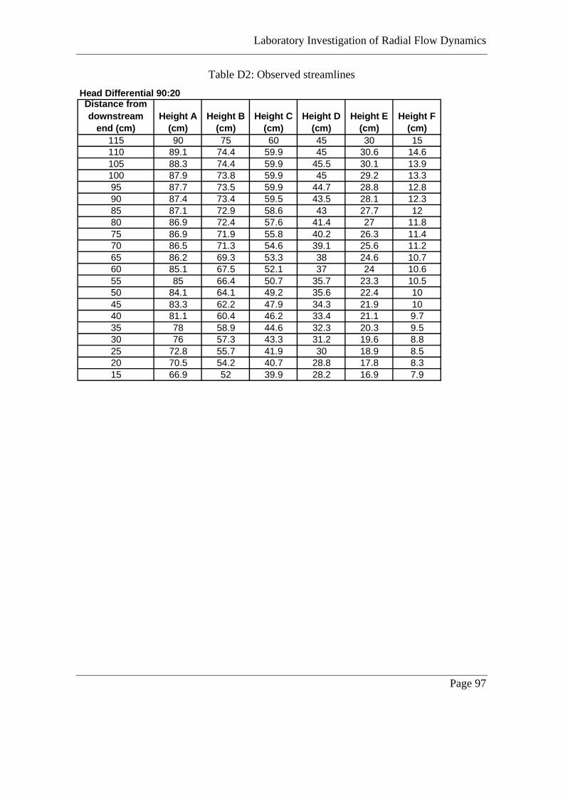
Laboratory Investigation of Radial Flow Dynamics
Page 97
Table D2: Observed streamlines
Head Differential 90:20Distance from downstream
end (cm)Height A
(cm)Height B
(cm)Height C
(cm)Height D
(cm)Height E
(cm)Height F
(cm)115 90 75 60 45 30 15110 89.1 74.4 59.9 45 30.6 14.6105 88.3 74.4 59.9 45.5 30.1 13.9100 87.9 73.8 59.9 45 29.2 13.395 87.7 73.5 59.9 44.7 28.8 12.890 87.4 73.4 59.5 43.5 28.1 12.385 87.1 72.9 58.6 43 27.7 1280 86.9 72.4 57.6 41.4 27 11.875 86.9 71.9 55.8 40.2 26.3 11.470 86.5 71.3 54.6 39.1 25.6 11.265 86.2 69.3 53.3 38 24.6 10.760 85.1 67.5 52.1 37 24 10.655 85 66.4 50.7 35.7 23.3 10.550 84.1 64.1 49.2 35.6 22.4 1045 83.3 62.2 47.9 34.3 21.9 1040 81.1 60.4 46.2 33.4 21.1 9.735 78 58.9 44.6 32.3 20.3 9.530 76 57.3 43.3 31.2 19.6 8.825 72.8 55.7 41.9 30 18.9 8.520 70.5 54.2 40.7 28.8 17.8 8.315 66.9 52 39.9 28.2 16.9 7.9

Laboratory Investigation of Radial Flow Dynamics
Page 98
Head Differential 90:40Distance from downstream
end (cm)Height A
(cm)Height B
(cm)Height C
(cm)Height D
(cm)Height E
(cm)Height F
(cm)115 90 75 60 45 30 15110 90 74.5 59.7 45 30.4 14.1105 89.1 74.7 59.8 45.1 30.4 13.5100 88.6 74.3 60 45.3 30.2 13.195 88.6 74.3 60.2 45.3 29.8 12.790 88.3 73.9 60 44.7 29.3 12.385 88.1 73.6 59.7 44.5 28.8 12.180 87.6 73.1 58.8 43.4 28.2 1275 87.6 73 57.7 42.1 27.8 11.970 87.6 72.5 56.7 41.4 27.5 11.965 86.9 72.3 55.5 40.9 26.9 11.760 86.4 70.6 54.6 40.2 26.6 11.755 85.9 69.4 54 39.3 26.3 11.950 85 68.6 52.9 38.7 25.8 11.645 83.9 66.9 52 38.1 25.5 11.640 83 65 51.4 37.5 25.1 11.735 81.8 63.9 50.5 37 24.6 11.130 80 62.8 49.7 36.3 24.3 10.725 77.9 61.1 49.3 35.9 23.8 10.320 75.9 59.8 48.5 35.9 22.9 1015 71.9 58 47.5 35.9 22.3 9.9

Laboratory Investigation of Radial Flow Dynamics
Page 99
Head Differential 90:60Distance from downstream
end (cm)Height A
(cm)Height B
(cm)Height C
(cm)Height D
(cm)Height E
(cm)Height F
(cm)115 90 75 60 45 30 15110 89.3 74.7 61 45.7 30.5 13.6105 88.7 74.7 61.3 46.1 30.2 13100 88.4 74.6 61.8 46.4 30 12.395 88.5 74.2 62.2 46.3 29.9 1290 88.2 74.5 62.4 45.8 29.8 11.685 87.9 74.5 62.1 45.5 29.5 11.580 87.9 74.4 61.9 45.3 29.1 11.975 87.9 74.7 61 44.4 28.7 11.670 87.9 74.5 60.3 43.8 28.5 11.865 87.7 74.1 59.6 43.6 28.5 11.960 87.1 72.6 59.5 43 28.5 11.755 86.9 72 59.3 42.7 28.6 12.150 86.5 71.2 58.5 42.5 28.1 1245 85.7 70.8 58 42.4 28.3 12.340 85 69.8 57.8 42.2 28.3 12.135 83.9 69 57.4 42.3 27.6 11.930 82.8 68.5 57.2 42.5 27.6 11.725 82 68.1 57.5 43 27.6 10.820 80.2 67.7 57.5 43 27.4 10.815 76.7 67 57.3 43.8 27.5 10.5

Laboratory Investigation of Radial Flow Dynamics
Page 100
The levels recorded in each of the standpipes is recorded below for the four head
differentials studied (Table D3).
Head Differential 90:70Distance from downstream
end (cm)Height A
(cm)Height B
(cm)Height C
(cm)Height D
(cm)Height E
(cm)Height F
(cm)115 90 75 60 45 30 15110 87 72.2 60.8 47.4 28.8 14.2105 86.6 71.2 61.8 47.6 28.7 13100 86.2 70.9 61.9 48.5 28.5 11.895 86.6 71.4 62.5 48.7 28.7 11.290 86.6 71.5 62.8 49.3 28.8 10.985 86.6 71.5 63.1 49.8 29.1 10.980 86.6 71.5 62.8 49.8 29.1 11.275 86.7 71.8 62.9 49.3 29.4 12.170 86.7 71.9 62.2 49.1 29.6 12.565 86.5 70.6 62.1 49 29.7 12.360 86.5 70 61.7 49 29.6 1355 86.3 69.6 61.6 49.1 29.7 12.950 86.2 69.4 61.9 48.9 30 13.545 85.7 69.4 61.6 49.2 30.5 13.840 85.5 68.5 61.5 49.3 30.3 13.935 84.7 67.5 61.5 49.9 30.5 13.730 84.2 67.9 61.9 50.7 30.3 13.525 83.2 68.1 62.5 51.3 30.2 12.920 81.4 68.2 63 52.2 30 11.915 78.2 68.4 63.8 53 30.4 11.6
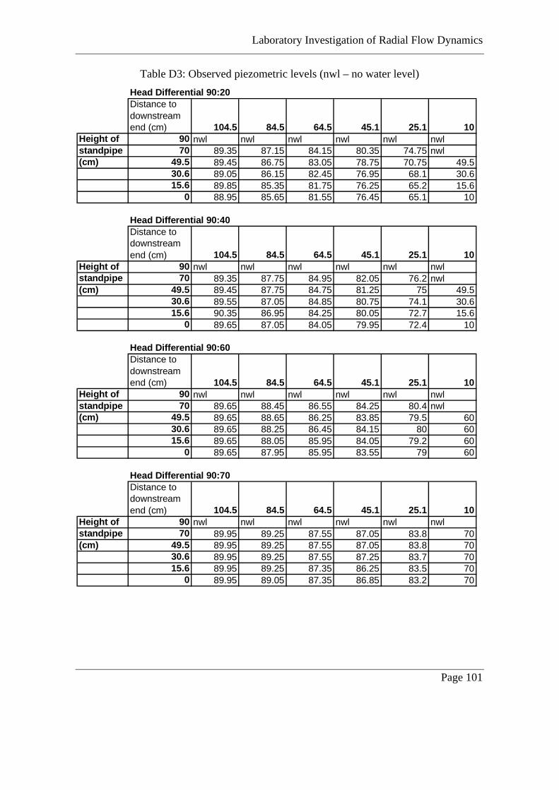
Laboratory Investigation of Radial Flow Dynamics
Page 101
Table D3: Observed piezometric levels (nwl – no water level)
Head Differential 90:20Distance to downstream end (cm) 104.5 84.5 64.5 45.1 25.1 10
Height of 90 nwl nwl nwl nwl nwl nwlstandpipe 70 89.35 87.15 84.15 80.35 74.75 nwl(cm) 49.5 89.45 86.75 83.05 78.75 70.75 49.5
30.6 89.05 86.15 82.45 76.95 68.1 30.615.6 89.85 85.35 81.75 76.25 65.2 15.6
0 88.95 85.65 81.55 76.45 65.1 10
Head Differential 90:40Distance to downstream end (cm) 104.5 84.5 64.5 45.1 25.1 10
Height of 90 nwl nwl nwl nwl nwl nwlstandpipe 70 89.35 87.75 84.95 82.05 76.2 nwl(cm) 49.5 89.45 87.75 84.75 81.25 75 49.5
30.6 89.55 87.05 84.85 80.75 74.1 30.615.6 90.35 86.95 84.25 80.05 72.7 15.6
0 89.65 87.05 84.05 79.95 72.4 10
Head Differential 90:60Distance to downstream end (cm) 104.5 84.5 64.5 45.1 25.1 10
Height of 90 nwl nwl nwl nwl nwl nwlstandpipe 70 89.65 88.45 86.55 84.25 80.4 nwl(cm) 49.5 89.65 88.65 86.25 83.85 79.5 60
30.6 89.65 88.25 86.45 84.15 80 6015.6 89.65 88.05 85.95 84.05 79.2 60
0 89.65 87.95 85.95 83.55 79 60
Head Differential 90:70Distance to downstream end (cm) 104.5 84.5 64.5 45.1 25.1 10
Height of 90 nwl nwl nwl nwl nwl nwlstandpipe 70 89.95 89.25 87.55 87.05 83.8 70(cm) 49.5 89.95 89.25 87.55 87.05 83.8 70
30.6 89.95 89.25 87.55 87.25 83.7 7015.6 89.95 89.25 87.35 86.25 83.5 70
0 89.95 89.05 87.35 86.85 83.2 70