Brigham Young University Brigham Young University

BYU ScholarsArchive BYU ScholarsArchive

Theses and Dissertations

2012-08-13

Laboratory Experiments on Colliding Nonresonant Internal Wave Laboratory Experiments on Colliding Nonresonant Internal Wave

Beams Beams

Sean Paul Smith Brigham Young University - Provo

Follow this and additional works at: https://scholarsarchive.byu.edu/etd

Part of the Mechanical Engineering Commons

BYU ScholarsArchive Citation BYU ScholarsArchive Citation Smith, Sean Paul, "Laboratory Experiments on Colliding Nonresonant Internal Wave Beams" (2012). Theses and Dissertations. 3300. https://scholarsarchive.byu.edu/etd/3300

This Thesis is brought to you for free and open access by BYU ScholarsArchive. It has been accepted for inclusion in Theses and Dissertations by an authorized administrator of BYU ScholarsArchive. For more information, please contact scholarsarchive@byu.edu, ellen_amatangelo@byu.edu.

Laboratory Experiments on Colliding Nonresonant Internal Wave Beams

Sean Smith

A thesis submitted to the faculty of

Brigham Young University

in partial fulfillment of the requirements for the degree of

Master of Science

Julie Vanderhoff, Chair

Daniel Maynes

Tadd Truscott

Department of Mechanical Engineering

Brigham Young University

December 2012

Copyright © 2012 Sean Smith

All Rights Reserved

ABSTRACT

Laboratory Experiments on Colliding Nonresonant Internal Wave Beams

Sean Smith

Department of Mechanical Engineering, BYU

Master of Science

Internal waves are prominent fluid phenomena in both the atmosphere and ocean. Because

internal waves have the ability to transfer a large amount of energy, they contribute to the global

distribution of energy. This causes internal waves to influence global climate patterns and critical

ocean mixing. Therefore, studying internal waves provides additional insight in how to model

geophysical phenomena that directly impact our lives.

There is a myriad of fluid phenomena with which internal waves can interact, including

other internal waves. Equipment and processes are developed to perform laboratory experiments

analyzing the interaction of two colliding nonresonant internal waves. Nonresonant interactions

have not been a major focus in previous research. The goal of this study is to visualize the flow

field, compare qualitative results to Tabaei et al., and determine the energy partition to the second-

harmonic for eight unique interaction configurations. When two non-resonant internal waves col-

lide, harmonics are formed at the sum and difference of multiples of the colliding waves’ frequen-

cies. In order to create the wave-wave interaction, two identical wave generators were designed

and manufactured. The interaction flow field is visualized using synthetic schlieren and the en-

ergy entering and leaving the interaction region is analyzed. It is found that the energy partitioned

to the harmonics is much more dependent on the general direction the colliding waves approach

each other than on the angle. Depending on the configurations, between 0.5 and 7 percent of the

energy within the colliding waves is partitioned to the second-harmonics. Interactions in which

the colliding waves have opposite signed vertical wavenumber partition much more energy to the

harmonics. Most of the energy entering the interaction is dissipated by viscous forces or leaves the

interaction within the colliding waves. For all eight configurations studied, 5 to 8 percent of the

energy entering the interaction has an unknown fate.

Keywords: internal waves, statified fluid, nonlinear interactions, wave-wave interactions nouniver-

sitypages

ACKNOWLEDGMENTS

Special thanks to all those who made the successful completion of this thesis possible.

My committee chair, Dr. Vanderhoff, has spent over a year teaching and supporting me in every

way. She has been extremely flexible, allowing me to choose the direction of my research. I

recognize the tremendous amount of time she has dedicated to my success. I extremely appreciate

the financial support she has found for me. I also offer thanks to the other members of my thesis

committee, Dr. Maynes and Dr. Truscott, for their willingness to review my thesis and dedicate a

portion of their busy lives to my success.

My colleagues, Benjamin Hillyard, Leo Latore, Tyler Blackhurst, Lauren Ebberly, Thomas

Evans and Matthew Marshall, have also dedicated a large amount of time to my project. Benj, Leo,

and Tyler have been my student guides at I have worked on this research. They have answered

questions and offered advice countless times. Lauren Ebberly taught me a great deal concerning

the lab and how to do internal wave experiments. Thomas Evans assisted in collecting and pro-

cessing data which saved me many hours. Matthew Marshall has been my technical guru offering

programing, software, and hardware support.

Above all, my wife, Jean, is my greatest supporter of all. She has and continues to emo-

tionally and financially support me in achieving my academic goals despite the impact it has on

her own life.

Appreciation is also extended to the Rocky Mountain NASA Space Grant Consortium for

the financial assistance it provided.

TABLE OF CONTENTS

LIST OF TABLES . . . . . . . . . . . . . . . . . . . . . . . . . . . . . . . . . . . . . . . vi

LIST OF FIGURES . . . . . . . . . . . . . . . . . . . . . . . . . . . . . . . . . . . . . . viii

Chapter 1 Introduction . . . . . . . . . . . . . . . . . . . . . . . . . . . . . . . . . . . 11.1 Internal Waves . . . . . . . . . . . . . . . . . . . . . . . . . . . . . . . . . . . . 1

1.2 Scope . . . . . . . . . . . . . . . . . . . . . . . . . . . . . . . . . . . . . . . . . 2

1.3 Theory . . . . . . . . . . . . . . . . . . . . . . . . . . . . . . . . . . . . . . . . . 5

Chapter 2 Literature Review . . . . . . . . . . . . . . . . . . . . . . . . . . . . . . . 112.1 General Background . . . . . . . . . . . . . . . . . . . . . . . . . . . . . . . . . 11

2.2 Experimental Setup . . . . . . . . . . . . . . . . . . . . . . . . . . . . . . . . . . 12

2.3 Wave Generation . . . . . . . . . . . . . . . . . . . . . . . . . . . . . . . . . . . 14

2.4 Interactions . . . . . . . . . . . . . . . . . . . . . . . . . . . . . . . . . . . . . . 15

2.5 Summary . . . . . . . . . . . . . . . . . . . . . . . . . . . . . . . . . . . . . . . 18

Chapter 3 Methods . . . . . . . . . . . . . . . . . . . . . . . . . . . . . . . . . . . . . 193.1 Wave Generator . . . . . . . . . . . . . . . . . . . . . . . . . . . . . . . . . . . . 19

3.1.1 Preliminary Design . . . . . . . . . . . . . . . . . . . . . . . . . . . . . . 19

3.1.2 Prototyping . . . . . . . . . . . . . . . . . . . . . . . . . . . . . . . . . . 22

3.1.3 Manufacturing . . . . . . . . . . . . . . . . . . . . . . . . . . . . . . . . 22

3.1.4 Testing . . . . . . . . . . . . . . . . . . . . . . . . . . . . . . . . . . . . 23

3.1.5 Characteristics of Waves Created by Wave Generators . . . . . . . . . . . 25

3.1.6 Wave Generator Design in Review . . . . . . . . . . . . . . . . . . . . . . 28

3.2 Experimental Setup . . . . . . . . . . . . . . . . . . . . . . . . . . . . . . . . . . 29

3.2.1 Experiment Preparation . . . . . . . . . . . . . . . . . . . . . . . . . . . 30

3.2.2 Synthetic Schlieren . . . . . . . . . . . . . . . . . . . . . . . . . . . . . . 32

3.2.3 Preliminary Uncertainty . . . . . . . . . . . . . . . . . . . . . . . . . . . 33

3.2.4 Lab Testing . . . . . . . . . . . . . . . . . . . . . . . . . . . . . . . . . . 34

3.2.5 Verification of Experimental Setup . . . . . . . . . . . . . . . . . . . . . . 36

3.3 Acquiring Data . . . . . . . . . . . . . . . . . . . . . . . . . . . . . . . . . . . . 38

3.3.1 Acquiring Data in Review . . . . . . . . . . . . . . . . . . . . . . . . . . 39

3.4 Data Processing . . . . . . . . . . . . . . . . . . . . . . . . . . . . . . . . . . . . 40

3.4.1 Energy Analysis . . . . . . . . . . . . . . . . . . . . . . . . . . . . . . . 41

3.4.2 Harmonic Flow Field . . . . . . . . . . . . . . . . . . . . . . . . . . . . . 45

3.5 Uncertainty Analysis . . . . . . . . . . . . . . . . . . . . . . . . . . . . . . . . . 45

3.5.1 Processing Uncertainty Analysis . . . . . . . . . . . . . . . . . . . . . . . 46

3.5.2 Measurement Uncertainty Analysis . . . . . . . . . . . . . . . . . . . . . 48

3.5.3 Statistical Uncertainty Analysis . . . . . . . . . . . . . . . . . . . . . . . 49

Chapter 4 Results . . . . . . . . . . . . . . . . . . . . . . . . . . . . . . . . . . . . . . 514.1 Qualitative Results . . . . . . . . . . . . . . . . . . . . . . . . . . . . . . . . . . 51

iv

4.2 Quantitative analysis . . . . . . . . . . . . . . . . . . . . . . . . . . . . . . . . . 58

4.2.1 Harmonic Wavenumbers . . . . . . . . . . . . . . . . . . . . . . . . . . . 58

4.2.2 Energy Partition . . . . . . . . . . . . . . . . . . . . . . . . . . . . . . . 61

Chapter 5 Conclusions . . . . . . . . . . . . . . . . . . . . . . . . . . . . . . . . . . . 735.1 Contributions . . . . . . . . . . . . . . . . . . . . . . . . . . . . . . . . . . . . . 74

5.2 Future Work . . . . . . . . . . . . . . . . . . . . . . . . . . . . . . . . . . . . . . 75

REFERENCES . . . . . . . . . . . . . . . . . . . . . . . . . . . . . . . . . . . . . . . . . 77

Appendix A Wave Generator Drawing Package . . . . . . . . . . . . . . . . . . . . . . 81

Appendix B Lab Procedures . . . . . . . . . . . . . . . . . . . . . . . . . . . . . . . . . 91

Appendix C Experiment Worksheet . . . . . . . . . . . . . . . . . . . . . . . . . . . . . 101

v

LIST OF TABLES

3.1 Major experimental setup parameters used in the oscillated cylinder experiment bySutherland et al. and used in the verification experiment done in this study. . . . . . 36

3.2 Number of data sets collected for each configuration. . . . . . . . . . . . . . . . . 393.3 Coordinates of vertices to define control volumes. . . . . . . . . . . . . . . . . . . 423.4 The measured values, uncertainty, and description of all variables used in process-

ing uncertainty analysis . . . . . . . . . . . . . . . . . . . . . . . . . . . . . . . . 473.5 Percent change in the energy crossing the four boundaries of a control volume

when moved 1 and 5 pixels left, right, up, and down. . . . . . . . . . . . . . . . . 49

4.1 Summary of whether a harmonic is seen propagating away from the interactionwithin the two-dimensional quadrants. . . . . . . . . . . . . . . . . . . . . . . . . 57

vi

LIST OF FIGURES

1.1 Perturbed fluid parcel in a linearly stratified fluid. . . . . . . . . . . . . . . . . . . 5

1.2 Relationship between frequency, angle of propagation, and wavenumbers. . . . . . 7

1.3 Structure of an internal wave being generated by corrugated topography. . . . . . . 8

2.1 SAR image showing internal waves being generated by rough topography. . . . . . 12

3.1 Schematic of a wave generator and how an internal wave is generated . . . . . . . 20

3.2 Cam designs ready for the laser printer and the finished cams on the shaft . . . . . 21

3.3 Completed wave generator. . . . . . . . . . . . . . . . . . . . . . . . . . . . . . . 23

3.4 Modifications made to the plate design. . . . . . . . . . . . . . . . . . . . . . . . 24

3.5 First test of two colliding wave beams. . . . . . . . . . . . . . . . . . . . . . . . . 24

3.6 Internal wave beam and other disturbances created by the wave generator. . . . . . 26

3.7 Characteristics of the waves produced by the generator. . . . . . . . . . . . . . . . 27

3.8 Lab setup for the relative positions of the camera, tank, and illuminated pattern. . . 29

3.9 Schematic of the double bucket method used to fill the experimental tank with a

linear density gradient. . . . . . . . . . . . . . . . . . . . . . . . . . . . . . . . . 31

3.10 Finding optimal distance from the tank to the pattern. . . . . . . . . . . . . . . . . 34

3.11 Test of a wave beam being damped by filter material. . . . . . . . . . . . . . . . . 35

3.12 ΔN2 (a) and N2t (b) fields for oscillating cylinder experiments performed by Suther-

land et al. [1]. . . . . . . . . . . . . . . . . . . . . . . . . . . . . . . . . . . . . . 37

3.13 ΔN2 (a) and N2t (b) fields for oscillating cylinder experiments performed in this study. 37

3.14 Primary and Secondary wave angles and directions for all configurations. . . . . . 38

3.15 Control volumes used to analyze configurations 1-4. . . . . . . . . . . . . . . . . . 42

3.16 Timeseries for four planes of a control volume. . . . . . . . . . . . . . . . . . . . 43

3.17 Energy spectra for four planes of a control volume . . . . . . . . . . . . . . . . . . 44

4.1 False color images of the internal waves interacting for configuration 1-4. . . . . . 53

4.2 False color images of the internal waves interacting for configuration 5-8. . . . . . 54

4.3 ΔN2 fields of the interaction filtered for the sum and difference second-harmonics

for configurations 1 and 2. . . . . . . . . . . . . . . . . . . . . . . . . . . . . . . 55

4.4 ΔN2 fields of the interaction filtered for the sum and difference second-harmonics

for configurations 3 and 4. . . . . . . . . . . . . . . . . . . . . . . . . . . . . . . 56

4.5 Power spectrum of the lone primary and secondary wave fields. . . . . . . . . . . . 58

4.6 Power spectrum of the interaction for configuration 1. . . . . . . . . . . . . . . . . 59

4.7 Power spectrum of the interaction for configuration 1 with the power spectra for

the primary and secondary waves subtracted. . . . . . . . . . . . . . . . . . . . . 60

4.8 Wavenumbers of colliding and second-harmonic waves . . . . . . . . . . . . . . . 61

4.9 Energy spectrums of incoming and outgoing energy for configuration 4. . . . . . . 62

4.10 Energy within the primary and secondary waves as they enter and leave the control

volume for all 16 runs of configuration 1. . . . . . . . . . . . . . . . . . . . . . . 63

4.11 Energy within the sum and difference second-harmonic for each experimental run

of configurations 1-4. . . . . . . . . . . . . . . . . . . . . . . . . . . . . . . . . . 64

viii

4.12 Energy within the sum and difference second-harmonic for each experimental run

of configurations 5-8. . . . . . . . . . . . . . . . . . . . . . . . . . . . . . . . . . 65

4.13 Energy partitioned to the sum and difference second-harmonics. . . . . . . . . . . 67

4.14 Energy partitioned to a third-harmonic in configurations 4 (a) and 8 (b). . . . . . . 67

4.15 Exponential curve fit to estimate energy from colliding waves in harmonics. . . . . 68

4.16 Adjusted energy partitioned to the sum and difference second-harmonics. . . . . . 69

4.17 Estimated outcome of all energy entering the interaction. . . . . . . . . . . . . . . 71

ix

CHAPTER 1. INTRODUCTION

1.1 Internal Waves

Although not visible to the naked eye, internal waves may be more abundant than com-

monly observed surface waves. Just like surface waves, internal waves can carry a tremendous

amount of energy. Contributing to the amount of energy an internal wave can transfer is its enor-

mous size. Internal waves can measure up to thousands of kilometers in wavelength and hundreds

of kilometers in amplitude in the atmosphere. In the ocean, internal waves can measure up to

hundreds of kilometers in wavelength and hundreds of meters in amplitude. Because of the large

scales of internal waves and the impact they have on global energy transfer, internal waves are

generally classified as geophysical phenomena.

The main reason for studying internal wave behavior is the associated energy. It is estimated

that 2.1 Tera watts of energy is required to maintain critical ocean mixing [2]. It is also estimated

that internal waves transfer and dissipate a large portion of that energy to the deep ocean resulting

in ocean mixing. Such ocean mixing is crucial. Ocean mixing disperses nutrients essential for

ocean life and maintains temperature distributions which affect global climate patterns. Similar

arguments about the effects of internal waves in the atmosphere can also be made.

Despite the prevalence of internal waves, relatively little is known about how they are

generated, interact with surrounding phenomena, and dissipate. In order for internal waves to exist

a stably stratified fluid is required. A stably stratified fluid is any fluid that becomes more dense

with increasing depth, such as the ocean and atmosphere. Internal waves are most commonly

generated when a stratified fluid flows over rough topography. Once internal waves have been

generated, there are a myriad of fluid phenomena with which they can interact. This includes

vorticies, mean flows, density discontinuities, solid boundaries, and other internal waves. Such

interactions could increase the size of the internal wave, transfer its energy to other fluid flow, or

cause the wave to partially or fully break.

1

1.2 Scope

As mentioned previously, internal waves can interact with numerous other fluid phenomena—

one of which is other waves. There have been many studies focusing on internal wave-wave inter-

actions, particularly resonant wave-wave interactions. These interactions occur when two internal

waves resonantly interact forming a third wave. In a resonant wave-wave interaction, all energy

from the two interacting waves is transfered to the third wave, resulting in only one wave after the

interaction. This type of interaction is often called a resonant triad. Resonant wave-wave interac-

tions were first introduced by Phillips [3] who found the relationship between the wavenumber,�k,

and frequency, ω , of interacting waves to be

�k1±�k2 =�k3, (1.1)

ω1±ω2 = ω3. (1.2)

Resonant wave-wave interactions have since been heavily studied on account of their ability to

transfer a large amount of energy to smaller scales. Their importance was made manifest by the

Garrett and Munk spectrum [4], a numerical model that describes internal wave energy distribution,

in which resonant wave-wave interactions dominate internal wave energy transfer.

Even though resonant wave-wave interactions have been heavily studied, nonresonant wave-

wave interactions have received little attention. As two nonresonant waves interact, harmonic

waves with frequencies at multiples of the sum and difference of the colliding waves’ frequencies

are generated, as described by

ωharmonic =| Aω1±Bω2 |, (1.3)

where A and B are integers. Unlike resonant wave-wave interactions, all the energy within non-

resonant colliding waves is not transfered to newly generated harmonics. However, it has been

shown the lower order harmonics, where A and B are minimized, tend to carry more energy than

higher order harmonics. In order for any harmonic to develop into a propagating internal wave,

the frequency of the harmonic must be less than the natural frequency of the fluid or Brunt-Vaisala

frequency (see §2). Assuming a harmonic frequency is less than the natural frequency of the fluid,

a harmonic wave will be formed and propagate away from the interaction region. In the case that

2

a harmonic frequency is greater than the natural frequency of the fluid, an evanescent wave is

formed. An evanescent wave in a nonpropagating wave. In other words, as the interacting waves

excite a harmonic frequency that is above the natural frequency of the fluid and energy is unable

to propagate away from the interaction. Instead, the energy will accumulate at that frequency and

may eventually cause overturning of the fluid.

Nonresonant internal wave interactions were observed as early as 1973 when McEwan [5]

crossed two internal waves while trying to discover the interacting wave’s effect on fluid strat-

ifications. He observed harmonic waves at frequencies according equation 1.3, but no further

interaction analysis occurred. Chashechkin and Neklyudov [6] also found harmonic frequencies

present in their experiments by inserting conductivity probes in and around the interaction region

of two colliding waves. However, they were unable to capture data for the complete flow field, so

their results are rather limited. Internal wave interactions were visualized by Teoh et al. [7], but

no harmonic internal waves were reported in this case due to symmetry and the harmonic frequen-

cies being higher than the Brunt-Vaisala frequency. Instead, energy accumulated in the evanescent

harmonics until the fluid eventually overturned. Javam et al. [8] performed numerical studies on

interacting internal waves and confirmed that if harmonic energy could not leave the interaction re-

gion in the form of propagating waves, overturning would ensue. On the other hand, if propagating

harmonic waves were formed, the harmonics would have frequencies in accordance with equation

1.3, and the stratification would not be destroyed by overturning. Numerical studies were also

performed by Huang et al. [9] who tracked the second-order sum harmonic (equation 1.3) as two

atmospheric enveloped waves collided. Their study focused on only one interaction and showed

that a substantial amount of energy can be transfered to harmonics. Tabaei et al. [10] derived

equations to predict the amplitudes of harmonics generated by two colliding internal wave beams

assuming weakly nonlinear theory. Their derivations predict that up to six first-order harmonic

waves are generated, all at different amplitudes, but do not account for turbulence or dissipation

within the interaction.

From an experimental point of view, there have historically been three main challenges

in attempting internal wave experiments: the preparation of a stratified fluid, the generation of

monochromatic internal waves, and the visualization of the flow field [11]. The first challenge, the

preparation of a stratified fluid, was resolved in 1965 by Oster [12] who developed the ”double

3

bucket” method. This method has become the standard for creating a stratified fluid in all internal

wave experiments and is described further in §3. Visualization of the flow field has also been

made possible by the development of particle image velocimetry to capture time resolved velocity

fields [13] and the synthetic schlieren method which tracks density perturbations in the flow field

[1, 14]. Both of these methods have proven successful when applied to internal wave experiments.

§3 provides detailed information on the synthetic schlieren method. The most recent challenge to

be overcome is the development of a method to generate monochromatic waves. Previous wave

generation methods consisted of oscillating bodies or paddle generators. Both of these methods

have proven difficult to use in experiments for three reasons: they create multiple wave beams,

a full-wave length is not generated, and powerful nonlinear harmonics are also emitted from the

generators. Gostiaux et al. [11] recently proposed a new wave generation method that in large

measure overcomes previous wave generation complications by forcing translating plates to move

together in a wave-like profile. This wave generation method is described in much more detail in

section §3.1.

Considering the outlined synopsis of previous studies on nonresonant internal wave inter-

actions and general internal wave experiments, the scope of this research is as follows:

• Design an experiment to analyze two interacting internal wave beams using the most

up-to-date methods. In the last few years a stratified flow lab at BYU has been developed

which includes using the “double bucket” method to create a stratified fluid and the syn-

thetic schlieren method to visualize the flow field. However, there has been difficulty in the

repeatability of implementing the “double bucket” method and the accuracy of the synthetic

schlieren visualization technique was not ideal. Furthermore, no stationary wave generator

has previously been implemented in this lab. Therefore, as part of this research, the pro-

cedures of applying the “double bucket” method are standardized to ensure repeatability of

creating a stratified fluid, the synthetic schlieren visualization method is enhanced to increase

accuracy of results, and two wave generators based on the design of Gostiaux et al. [11] are

design and manufactured.

• Analyze second-order harmonic waves generated for 8 wave-wave interaction configu-

rations. One of the interesting aspects of interacting internal waves are the harmonics that

4

are generated within the interaction. The generation and intensity of these harmonics are

dependent on the the orientation of the interacting waves. Multiple configurations of collid-

ing waves must be studied in order to understand the complete spectrum of internal wave

two-dimensional collisions. The partition of energy to the second-harmonic is found, as well

as, the overall dissipation of energy with the interaction.

• Compare qualitative results to predictions by Tabaei et al. [10], who derived a theory to

estimate the outcome of two colliding waves.

1.3 Theory

Internal waves can only exist in stably stratified fluids, meaning the fluid becomes more

dense as depth increases. The stratification causes each fluid parcel to have a neutrally buoyant

depth. If any fluid parcel is perturbed up or down, the fluid particle naturally wants to return to

its neutrally buoyant depth. This tendency for perturbed fluid parcels to return to their neutrally

buoyant state is the condition that makes it possible for internal waves to exist. The frequency that

a perturbed fluid parcel oscillates as the parcel tries to return to its naturally buoyant state is known

as the buoyancy frequency, or Brunt-Vaisala frequency, and is denoted by N.

δz

δρ

z

ρ(z)

Figure 1.1: A fluid parcel perturbed δz into fluid that is δρ from its hydrostatic state. The slanted

line represents the fluid density as a function of height.

5

The buoyancy frequency can be easily derived from Newton’s laws. Suppose a fluid parcel

of density ρ0 is initially at a vertical level z0 in a motionless fluid where density increases linearly

with depth. If the parcel is vertically displaced by a distance δz, Figure 1.1 shows the difference of

the fluid parcel’s density compared to the surrounding fluid δρ . Newton’s laws predict the motion

described by

ρ0d2δz

dt2=−δρg. (1.4)

Because the displacement distance is considered to be small, δρ can be approximated in terms of

δz:

δρ �−dρdz

δz. (1.5)

Substituting 1.5 into 1.4 gives the differential equation

d2δz

dt2− g

ρ0

dρdz

δz = 0, (1.6)

which is recognizable as the spring equation, where the natural frequency can be described as

N =

(− g

ρ0

dρdz

)1/2. (1.7)

A similar analysis can be made with a fluid parcel being displaced along a line at an angle

θ from the vertical. Such an analysis reveals vertical oscillations with the frequency

ω = N cos(θ). (1.8)

If the oscillations are vertical, θ = 0 causing ω to equal N. Any forcing frequency higher than N

creates waves that are unable to propagate in any direction. As already mentioned, these waves are

termed evanescent.

Equation 1.8 can be used to find the dispersion relation in a linearly stratified fluid. The

dispersion relation for any wave describes how the frequency depends on the wavenumber. Figure

1.2 illustrates this dependency. The diagonal fluid oscillations at angle θ are parallel to the phase

lines, making the wavenumber vector,�k, perpendicular to these lines. The wavenumber vector also

forms and angle θ to the horizontal in wavenumber space [15]. The dispersion relation for the

6

z

x

k

θ

θ

k

m

k

Figure 1.2: The left figure shows an internal wave with its crests (solid lines), troughs (dotted

lines), and oscillating fluid motion direction, at an angle θ from the vertical. The wavenumber�k is

perpendicular to the phases. In the right figure the wavenumber vector makes an angle θ with the

horizontal in wavenumber space [15].

two-dimensional x-z plane is

ω2 = N2 k2

k2 +m2, (1.9)

where k and m are the horizontal and vertical wavenumbers respectively.

The dispersion relation is one of the fundamental concepts in the study of internal waves,

and likewise has a very important role in this experimental study. The dispersion relation is used

to determine the direction of energy propagation from the generators. As seen from equation 1.8, a

change in the excitation frequency not only changes the frequency of the phase oscillations but also

the angle at which the wave propagates. Careful planning during experimental setup is required for

each experiment to ensure the generated wave is propagating at the appropriate angle and direction.

One of the keys to conceptually understanding internal waves is knowing how they prop-

agate. Unlike a surface wave, the wave phases and wave energy do not propagate in the same

direction. In fact, the wave phases and wave energy must propagate orthogonal to each other in

order to satisfy the Navier-Stokes equations. Figure 1.3 shows the structure of an internal wave,

including the direction of phase and energy propagation, being generated over corrugated topogra-

7

Figure 1.3: An internal wave generated as fluid flows over continuously corrugated topography.

Important wave structure component are labeled in figure.

phy. The speed and direction of the propagating wave phases are described by the phase velocity,

�c. The phase velocity for any multi-dimensional wave is given by

�c =ω|�k |2

�k (1.10)

If the dispersion relation (1.9) is applied to the phase velocity definition, the phase velocity for

two-dimensional internal waves is found:

�c =Nk

cos2(θ)(cos(θ),sin(θ)). (1.11)

Although more difficult to visualize, the group velocity represents that velocity at which

energy is transported and is defined by �cg = ∇�kω . Again, applying the dispersion relation gives

the group velocity. For two-dimensional flow the group velocity is described by

�cg =Nk

sin(θ)cos(θ)(sin(θ),−cos(θ)). (1.12)

Figure 1.3 shows an example of the direction of phase and energy propagation for the wave gener-

ators used in this study.

8

As with any fluid phenomena, internal waves can be described using momentum, conserva-

tion of mass, and conservation of energy equations. In the case of internal waves, these equations

can be simplified using the Boussinesq approximation. The Boussinesq approximation simplifies

the equations in such a way that the dynamics of waves are preserved, while removing other den-

sity based dynamics, such as sound [15]. This approximation is made by ignoring all density terms

in the governing equations, except those that are multiplied by gravity. Since internal waves are

driven by the relationship between density and gravity, all internal wave dynamics are preserved

in the governing equations. For two-dimensional motion with the Boussinesq approximation, the

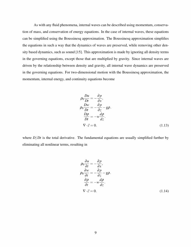
momentum, internal energy, and continuity equations become

ρ0DuDt

=−∂ p∂x

,

ρ0DwDt

=−∂ p∂ z−gρ.

DρDt

=−wdρdz

.

∇ ·�c = 0. (1.13)

where D/Dt is the total derivative. The fundamental equations are usually simplified further by

eliminating all nonlinear terms, resulting in

ρ0∂u∂ t

=−∂ p∂x

,

ρ0∂w∂ t

=−∂ p∂ z−gρ.

∂ρ∂ t

=−wdρdz

.

∇ ·�c = 0. (1.14)

9

CHAPTER 2. LITERATURE REVIEW

2.1 General Background

Internal waves were first reported in the early twentieth century in the form of fluctuations

of velocity and temperature in mean oceanic flows [16]. Preliminary studies began in the 1950’s

and 1960’s which added to the interest of internal waves until momentum was really gained in

the 1970’s. In the mid-1970’s Briscoe [17] described a conglomeration of internal wave papers

in the Journal of Geophysical Research as a kind of birthday for internal waves. Arguably one

of the greatest contributions to the study of internal waves was made by Garrett and Munk who

numerically calculated the distribution of oceanic internal wave energy in wave number–frequency

space [4]. This model has been universally named by the internal wave community as the Garret

and Munk spectrum and was later revised to be more accurate [18].

Rattray [19] published one of the early articles on the generation of internal waves. He

developed equations describing the generation of propagation of internal waves due to tides along

an idealized coast. Baines [20] shortly followed suite but focused on a numerical model for the

generation of internal waves due to tides over continental shelfs. This work was bolstered by

Lee and Beardsley [21] performing laboratory experiments on the generation of internal waves

by ocean ridges and comparing the laboratory results to numerical models. From the time of

these early publications, there have been an innumerable about of internal wave studies trying to

describe the how internal waves are formed [22, 23]. The majority of these studies focus on the

generation of internal waves by some form of rough topography. Observational data from the

ocean and atmosphere confirms that there is a large increase in internal wave activity around rough

topography [24,25]. Figure 2.1 shows internal waves represented by the dark and light bands being

formed by rough topography [26].

Early laboratory internal wave experiments were mainly qualitative due to a lack of means

to capture quantitative information [27, 28]. Only in the last 15 years have laboratory experiments

11

Figure 2.1: The image on the left shows dark and light bands representing internal waves capture

by synthetic aperture radar in the Gulf of California. The image on the right is the bathometry for

the same location and labels eight separate wave groups found in the SAR image [26]. The internal

wave group associated with the ‘D’ label is pointed out by the arrow.

produced many quantitative results. Many numerical studies have been made on internal waves,

especially simplified linear studies using ray theory [29]. Nonlinear models have recently become

increasingly popular as computational power increases [8, 30, 31]. Given the scope of this study,

this literature review will focus on studies relating to the experimental setup, generation, and inter-

action of internal waves.

2.2 Experimental Setup

Oster [12] is likely one of the most cited articles in internal wave experimental setups

because of his description of how to create a stratified fluid. Oster introduced three ways of creating

12

a linearly stratified fluid in an experimental tank. The first method was to fill the tank first with

a dense fluid and then add a less dense fluid on the surface of the dense fluid. If the fluids are

miscible, over a long period of time the boundary between the to layers will gradually spread until

a linear density gradient is formed. The major draw back of this method is the large amount of

time required for the fluids to diffuse into the stratification. The second method consisted of using a

centrifuge to distribute denser fluid to the outside of spinning tank and less dense fluid to the center.

The disadvantage to this method is that the fluid must be spinning at the time of any experiment,

which makes it largely unusable in internal wave experiments. The third method, which has been

termed the “double bucket” method, was the most viable for internal wave experiments. This

method consisted of adding increasingly dense fluid to the bottom of the tank. A modified “double

bucket” is used in our study which adds decreasingly dense fluid to the surface of the experimental

tank as described in detail in §3. Variations to the “double bucket” method have more recently

been created that allows for nonlinear stratification to be created [32, 33].

Dalziel et al. [14] reviewed early internal wave visualization methods and presented the

fundamentals for the synthetic schlieren method. Classical schlieren was the first method used to

visualize internal waves. Classical schlieren utilized a large parabolic mirror and a light source to

create a field of parallel light rays passing through the experimental tank. The rays bend toward

areas of higher refractive index as they pass through the tank. By using a second parabolic mirror,

a knife edge, and a lens the resulting ray field creates an images on a screen. This method required

very large expensive parabolic mirrors and considerable care to setup. The Moir fringe method

consisted of multiple horizontally lined masks behind and in front of the experimental tank. When

the fluid is not perturbed, the masks line up one behind the other, appearing as if there is only one

mask. As the stratification is perturbed, the masks differential themselves causing the perturbation

to become visible. The major draw back to this visualization method is that the spacing in the

horizontally lined masks must be customized to the exact stratification currently in the tank. This

made the Moir fringe method highly impractical. The synthetic schlieren visualization method

was considerably simpler than previous methods and allowed quantitative results to be found.

Variations of the synthetic schlieren method included the use of horizontal lines as a background

pattern or a random pattern of dots.

13

Because of the finite size of experimental tanks, damping undesirable internal waves due to

reflection or other sources has been a challenge in internal wave experiments. McEwen [5] used a

combination of what was described as a “horizontal slotted absorber” and brass wire mesh, but still

recorded reflecting waves. Other damping methods consisted of trapping the waves in unused parts

of the experimental tank as done by Baines [27]. More recently, Peacock et al. [34] and Zhang et

al. [35] have successfully damped unwanted waves using Blocksom filter matting. Blocksom filter

matting is a HVAC filter material that is made from strands of interwoven fibers.

2.3 Wave Generation

An estimated 30% of the 3.7 TW of tidal energy is thought to generate ocean internal waves

according to Garrett and Kunze [36]. The primary site of internal wave generation in the ocean is

along rough topography on the ocean floor. In addition to topography generated waves, Fritts and

Alexander [37] described convective generation, shear generation, geostrophic adjustment, and

wave-wave interactions as other sources for internal wave generation.

The majority of previous laboratory experiments have focused on internal wave generation

over different types of topography. Sutherland and Linden [38] analyzed internal wave generation

as a stratified fluid flowed over a thin barrier or “knife edge”. Aguilar et al. [39] characterized

internal wave generation for flow over sinusoidal topography. Similarly, Echeverri et al. [40] os-

cillated a single Gaussian ridge in a stratified fluid to simulate internal wave generation due to

tidal motions. There have also been a number of laboratory experiments involving internal wave

generation not due to topography. Examples include Anson and Sutherland’s [41] study involving

internal wave generated by convective plumes and Flynn and Sutherland’s [42] study on internal

wave generation by gravity currents. Anson and Sutherland found that approximately 4% of the

energy within the plume was partitioned to the formation of internal waves. Flynn and Sutherland

found the internal waves are formed by the head of the intrusion forcing through the fluid.

For all experiments that do not focus on internal wave generation, but on some other aspect

of the propagation and dissipation of the wave, an internal wave must still be generated. Typical

means for this type of wave generation have been oscillating cylinders, paddle-like generators,

and wave motion generators. Oscillating cylinders are one of the earliest internal wave generation

methods and was used by Mowbray and Rarity [28], Dauxois et al. [43], and Peacock and Tabaei

14

[44]. Paddle-like generators consist of multiple blades that traverse back and forth excite a wave.

Teoh et al. [7] used two of these wave generators when analyzing internal wave interactions and

Gostiaux et al. [45] used this type of wave generator to analyze waves reflecting from slopes.

The most recent internal wave generation method was proposed by Gostiaux et al. [11]. Their

study described limitations of the oscillating cylinder and paddle-like generators. Some of these

limitations include the generation of multiple waves and strong harmonics by the generators. The

proposed generator consisted of plates being driven so that their profile created a wave motion (see

3.1). Further studies by Mercier et al. [46] supported that this newly proposed wave generation

method is superior to previous methods.

2.4 Interactions

Once internal waves have been generated, there are a myriad of phenomena with which they

can interact. For example, Mathur and Peacock [47] performed a numerical and experimental study

where internal waves interact with nonlinear stratifications. Such an interaction caused the wave to

be amplified, some to the point of overturning and breaking, or dissipated to the background flow.

Reflection also occurred when a wave collided with quickly changing density gradients. If the

changing density gradient caused the buoyancy frequency to equal the frequency of an approaching

wave, the wave’s energy was dissipated. This location in a density gradient is termed the critical

layer.

Another disturbance with which an internal wave can interact is a vortex and has been

studied by Godoy-Diana et al. [48]. They found that as the wave interacts with the vortex, the

wave acts as if it reached either a turning point, where the wave is completely reflected, or a critical

layer. Blackhurst [49] extended this work by creating a three-dimensional model of the interaction.

He used ray theory to simulate a wave approaching the vortex for a variety of situations, and his

results compared well to those by Godoy-Diana et al.

A popular interaction to study is internal waves colliding with solid boundaries. Peacock

and Tabaei [44] visualized waves colliding with slopes at a variety of angles representing topog-

raphy or a continental shelf. Strong reflections were reported in most cases and harmonics were

found propagating from the interaction site. Gostiaux et al. [45] continued the investigation by

finding quantitative results such as amplitudes. The energy within the second harmonic was found

15

in Fourier space. They were even able to detect an evanescent harmonic. Rodenborn et al. [50] did

a similar study and compared the reflected harmonic wave characteristics with theories presented

by Thorpe and Haines [51] and Tabaei et al. [10]. For some situations one or both of the theories

compared well to the experimental results. For other situation, neither theory could accurately

predict the observed outcome.

As mentioned previously, resonant wave-wave interactions have received a great deal of

attention. Phillips [3] is responsible for first bringing resonant interactions to the attention of

geophysicists. He identified the frequency combinations the make up resonant interactions. Muller

et al. [31] reviewed the general approach to find nonlinear resonant interaction solutions. McComas

and Bretherton [52] classified three forms of resonant interactions as induced diffusion, elastic

scattering, and parametric subharmonic instability. Induced diffusion consists of a low-frequency

wave interacting with a wave of much larger wavenumber and frequency. Elastic scattering is

when two waves of nearly the same horizontal wavenumbers, opposite vertical wavenumbers, and

close to identical frequencies interact. Parametric subharmonic instability is when two waves of

opposite wavenumber and equal frequencies resonate. Very few laboratory experiments have been

performed on these resonant interactions.

Resonant internal wave interactions became the center of attention when Garrett and Munk

formulated a model predicting resonant interactions to dominate internal wave energy transfer

within the ocean [4, 18]. Many researchers since have found evidence to support the Garrett and

Munk model but others are not so sure. Lvov, Polzin, and Yokoyama [53] have identified inconsis-

tencies concerning resonant interactions that put aspects of the Garrett and Munk model at serious

risk.

Martin, Simmon, and Wunsch [54] performed one of the early resonant interaction lab-

oratory experiments. Their goal was simply to experimental show that two waves theoretically

capable of creating a resonant interaction, would indeed resonate. The experiments used conduc-

tivity probes to measure density fluctuations. They not only showed that resonant interaction do

exist but found that the resulting waves were remarkably Strong.

As far as nonresonant wave-wave interaction studies, there have been relatively few. The

first notable record of a nonresonant interaction was performed by McEwan [5] as he tried to find

how wave-wave interactions affected the fluid density gradient. He reported observing harmonic

16

waves that were stronger than expected. Challenges in the laboratory setup and lack of advanced

visualization techniques leaves the results of this study to be vague. However, it was clear that

nonlinear internal wave interactions can lead to overturning and turbulence in the flow.

Over a decade and a half later, Chashechkin and Neklyudov [6] performed experiments

on nonlinear nonresonant interactions of internal waves in exponentially stratified fluid. Their

visualization techniques were also extremely limited so most of their data was recorded by inserting

a conductivity probe into regions in and around the interaction. The conductivity probes were used

to record density fluctuations within the fluid. Although proven to be fairly accurate, conductivity

probes are an intrusive measurement and only provide information at a single point. Spectral

analysis of the conductivity probes’ results indicated the presence of harmonic waves at frequencies

ω1−ω2, 2ω1−ω2, ω1−2ω2, and 3ω1−2ω2. Much more could be learned by visualizing the entire

flow field of the interaction.

Teoh et al. [7] developed an experiment that analyzed two symmetric colliding nonresonant

waves. Symmetric in this instance means the two colliding waves had the same frequency, and

thus approached each other at the same angle. The authors did a very good job at describing the

evolution of the interaction in terms for density gradient, velocity field, and turbulence. The flow

field was visualized using classical schlieren techniques. Due to the symmetry of the interaction,

the harmonic at frequency ω1−ω2 did not exist and all harmonics containing the addition of

the colliding waves’ frequencies were above the buoyancy frequency of the fluid, making them

evanescent. The build up of energy in these harmonics is what eventually led to turbulence within

the interaction. Javam et al. [8] followed up on Teoh’s experiment by doing a numerical simulation

on a symmetric and nonsymmetric wave-wave interaction. The symmetric case showed similar

results to Teoh. When the waves were nonsymmetric, harmonics at the expected frequencies were

formed. Because energy within the harmonics could propagate away, the interaction did not lead

to turbulence. Additional experiments with nonsymmetric waves would be useful.

The only theory this author found that predicts that outcome of two colliding nonresonant

waves was presented by Tabaei et al. [10]. In this theory, the authors assumed weakly nonlinear

waves were colliding, in other words, only the first few nonlinear terms were used to find the

solution. A detailed method was presented that describes the generated second harmonics. Also,

the third harmonic is shortly discussed, but the solution method was largely the same as finding

17

the second harmonics. Diagrams were shown that illustrate the generated harmonics for all two-

dimensional collision configurations. There were up to six second harmonics generated for each

configuration. Each generated harmonic traveled in up to four different directions away from

the interaction site. A solution method was also shown for when evanescent harmonics were

produced. As with many theories, this theory used approximations to arrive at a solution. For

example, inviscid principles were applied and only lower order nonlinear terms were included.

Most theories presented in the internal wave community have been compared with experimental

results; however, this theory has not been exposed to such a study. It would be advantageous to

compare these theoretical results to findings in a laboratory study.

The most recent study of note concerning interaction waves was published by Huang et

al. [9]. This is a fully nonlinear numerical study of two enveloped waves interacting. The particular

goal of the authors was to analyze the second sum harmonic (ωharmonic = ω1 +ω2). The study

examined the waves before, during, and after the interaction. A considerable amount of energy

was transfered to the harmonic. Therefore, the authors suggested that nonresonant wave-wave

interactions may be compared in importance to resonant wave-wave interactions. They found that

the energy of the produced harmonic is highly dependent on the orientation of the colliding waves.

2.5 Summary

The above review is a complete compilation of all articles found by the author concerning

nonresonant interactions, which indicates that the depth of understanding nonresonant interactions

is rather limited. Laboratory experiments have been performed and harmonics have been observed

[6]. These harmonics have only been analyzed using conductivity probes which only collect data

at a single point and are intrusive. Nonintrusive measurement methods have been used to observe

the flow field but only when evanescent harmonics are generated [7]. No laboratory experiments

have been performed to visualize and analyze the entire flow field when colliding waves generate

propagating harmonics. Furthermore, no experiments have corroborated the predictions by Tabaei

et al. [10]. This is the void this study seeks to fill within the scientific community.

18

CHAPTER 3. METHODS

The methods of this thesis are categorized in the following sections: wave generator, ex-

perimental setup, acquiring data, data processing, and uncertainty analysis.

3.1 Wave Generator

The basic design for the wave generator was inspired by descriptions of wave generators

used in previous experiments. Gostiaux et al. [11] originally proposed this type of wave generation

which consists of horizontal plates stacked on each other with a rotating camshaft traversing ver-

tically through the center (Figure 3.1). The rotating camshaft causes the plates to move back and

forth horizontally in a sinusoidal motion, which creates an internal wave beam. Recent studies on

this type of wave generator have shown it is ideal for studying nonlinear wave-wave interactions

because of its spatial and temporal monochromaticity [11, 46]. Another advantage to this form of

wave generation is that it ideally only creates one internal wave beam, although, as will be seen,

this is not necessarily true. Previous means of wave generation create multiple strong wave beams.

Any additional wave beams would need to dampened, which can often be difficult. Without the

detailed designs of these wave generators and because this experiment had different requirements

than any previously performed experiments, a new wave generator was designed.

3.1.1 Preliminary Design

Initial design considerations were centered around the spatial constraints of the experimen-

tal tank. The wave generator needs to fill the whole experimental thickness to ensure the resulting

waves were as two-dimensional as possible. The height of the generated wave beam can not be too

large or the interaction region would be too large to capture. The wave generator also needs to be

able to reach the bottom of the tank while being driven by a motor above the surface.

19

Figure 3.1: The left side of the image shows cams attached to a rotating shaft which drives hori-

zontal plates in a sinusoidal motion. The right side shows how an internal wave generated by the

motion of the plates [46]. In this figure vθ is the phase velocity and vg is the group velocity.

The next design considerations focused on the functionality, manufacturability, and assem-

bly of the wave generator. All the components of the wave generator need to be able to withstand

salt water conditions for an extended period of time and be easy to manufacture and assemble.

Aluminum has already proven to not corrode in our tank during previous experiments. However, a

wave generator made completely out of aluminum would be excessively heavy. Acrylic does not

corrode in salt water, is relatively light (especially in water), and is extremely easy to cut using a

laser cutter. It was decided that acrylic would work perfectly for the moving plates of the generator

and the structural components would be made out of aluminum.

The main concern with regards to the functionality of the wave generator was how to make

the plates move easily. One previously manufactured wave generator consisted of plates made out

of PVC with lead weights added to each plate until they were neutrally buoyant and would not

rub each other [11]. This design seemed needlessly difficult. With limited information about other

previously manufactured wave generators, a novel method needed to be independently conceptual-

ized. Glass balls placed between each plate in groves parallel to the motion direction would allow

each plate to easily move independently. However, this concept needed to be tested before the

complete wave generator was made.

The greatest manufacturing issue was how to manufacture and assemble the cams. It was

initially planned to manufacture the cams out of aluminum. Each cam would have a set screw to

20

hold it at a 45 degree angle rotation around the shaft from the cam directly below it (45 degree

rotations of the cams create a full wave period over nine plates). However, the time required

to machine nine identical cams and then orient them correctly on the shaft seemed tedious and

time consuming. Upon rethinking the design, an alternative solution was found that simplified the

manufacturing and assembly considerably. Along the length of the shaft where the cams were to

be attached, the side of the shaft could be milled down so the cross section of the shaft resembled a

semicircle. The cams could easily be cut out of 1/8 inch thick acrylic on the laser cutter. The shaft

hole in the cams could be cut to the same shape and size as the semicircular profile of the shaft.

The shaft hole in each of the cams could be rotated by 45 degrees (Figure 3.2(a)). The cams could

then slide onto the shaft and already be rotated 45 degrees from the adjacent cams (Figure 3.2(b)).

It was hoped that very close tolerances between the cams and shaft would keep the cams in place.

(a) (b)

Figure 3.2: Four cam designs ready for the laser printer (a). A 45 degree rotation has been applied

to each of the holes in the cams. The finish cams spiraling down the shaft (b).

This design is significantly easier than machining each cam by hand and manually setting

the angles. The laser cutter can cut all the cams in a few minutes and the rotation of the shaft hole

is easily done in any drawing program. If the new design worked, considerable time would be

saved in manufacturing.

One of the major advantages to the overall wave generator design is that it can easily be

altered in the future. Plates can be added or taken away, the plates can be switched out for larger or

21

thinner plates, and the amplitude of the plate motion can be altered. This creates great versatility

for future use of these wave generators in other experiments. Complete drawings of the wave

generator can be found in Appendix A.

3.1.2 Prototyping

The part of the wave generator design that was most in question was whether the glass beads

would allow the plates to move independently and a large force would not be required to move the

plates. Two acrylic plates were first made and tested using the beads. One plate was placed on the

other place with four beads in shallow channels along the desired direction of movement between

the plates. The upper plate proved to move easily over the beads with little force. It is interesting

to note that in most cases the beads did not actually role but the friction between the acrylic plates

and the glass beads was low enough that the plates slid across the beads. Nevertheless, the test was

a success and plans were made to manufacture a complete wave generator.

3.1.3 Manufacturing

The acrylic plates and cams were manufactured first. The laser cutter proved very efficient

in cutting the acrylic. A CNC mill was utilized to cut the channels for the beads in the acrylic

plates. The top and bottom casing plates were manufactured out of aluminum. The four support

beams were also manufactured out of aluminum. Holes were drilled every couple of inches along

the length of the support beams. These holes allowed a rod to be through the front and back beams.

The rod then sat on the top of the walls of the tank. The rod could be moved up and down through

the different holes so the wave generator can sit at different depths in the tank. At the top of the

beams an addition aluminum plate was used as a motor mount. The shaft extends from the plates

up to the motor. A sleeve with set screws was manufactured to attach the motor to the shaft. As

planned, the cams fit tightly around the shaft by friction. As a precaution, water resistant glue was

also used to keep the cams from moving. A completed wave generator is illustrated in Figure 3.3.

22

Figure 3.3: Left: The completed wave generator. The nine acrylic plates are at the bottom of the

generator and 4 supports extent up to the top motor mount plate. A shaft extends from the motor

to the cams within the plates. Top Right: Close up image of the nine plates creating a sinusoidal

profile. Bottom Right: Transparent depiction of a wave generator allowing the cams inside the

plates to be seen.

3.1.4 Testing

When the wave generator was near completion preliminary testing was performed. It was

quickly found that the size of the holes through the plates did not allow the cams to complete

their full revolution as the shaft turned. Although this was a potentially huge issue, only a slight

modification to the plates was required. The already manufactured plates were altered by widening

the width of the hole (Figure 3.4(b)). With the modified plates the wave generator worked without

incident. A step motor allowed the plates to be driven at a wide range of speeds. The plates moved

in and out of the wave generator to create one full wave length. With the success of the first wave

generator, a second wave generator was manufactured.

The next step to testing was ensuring the wave generators worked in a stratified fluid to

create internal waves. Figure 3.5 shows an image during preliminary testing of two colliding wave

23

(a) Original Plates (b) Modified Plates

Figure 3.4: Changes made to the plates after testing (not to scale).

Pixels

Pixels

100 200 300 400 500 600 700 800

100

200

300

400

500

600

700

Figure 3.5: A false color image of two wave beams colliding during initial testing. The wave beams

originate just off the image on the lower right and lower left side, and propagate in the direction of

the arrows.

beams. This false color image, as well as all false color images following, represents density

perturbations within the flow field. The wave beams originate just off the image in the bottom

left and right, and propagate in the directions shown by the arrows. The waves then collide at the

center of the image and continue out of the field of view. The phases of the waves can easily be

24

seen as the strands of color along the length of each beam. The wave generators clearly create well

defined internal wave beams.

3.1.5 Characteristics of Waves Created by Wave Generators

Although a comprehensive study of the wave generator is not the purpose of this study, it

is important to understand how different aspects of the wave generator affect characteristics of the

generated wave. An in depth study has previously been performed on similar wave generators by

Mercier at al. [46]. Their study explored the effects of changing the amplitude, frequency, angle

of emission, and discretization of the wave generator ( of plates used). Results showed that over

a range of amplitudes and frequencies, the wave generators produced waves that matched very

closely to numerical predictions.

Mercier at al. showed that the quality of the generated wave is directly dependent on the

angle of emission. Angle of emission refers to the angle that the wave comes off the wave generator

with respect to the oscillating plates as shown in Figure 3.6. This figure shows a wave generator

laid over a flow field at the wave generator’s approximate actual location. The angle of emissions

is labeled, as well as, other secondary and tertiary disturbance caused by the wave generator which

will be discussed shortly.

The angle of emission can be altered by changing the forcing frequency of the generated

wave or by changing the orientation of the wave generator. An ideal experimental setup would

change the angle of the wave generator to coincide with the angle of the propagating wave, causing

the angle of emission to be zero. However, the authors concluded that the quality of the generated

wave diminishes minimally for angles of emission up to 45 degrees. Therefore, considering the

waves in this study are only at shallow angles from the horizontal, there was no need to deal with

the tediousness of tilting the wave generators.

Discretization of the wave generators was also an issue addressed by Mercier et al. Dis-

cretization of the wave generator refers to the number of plates used to create each wave length of

the generated wave, M. They specifically studied two cases were M = 4 and M = 12. For both

cases, and despite the coarse discretization of the M = 4 case, the generated waves were smooth

and compared well to theory. However, the most notable difference was the presence of a sec-

ondary wave for the M = 4 case. The presence of this secondary wave is not wanted. In another

25

Primary Wave

Secondary Wave

Tertiary Wave

Angle of Emission

Figure 3.6: Flow field produced by the wave generator. Schematic of wave generator at approxi-

mate location is overlaid on the flow field. Multiple wave beams are emitted by the wave generator

at a given angle of emission.

study by Rodenborn et al. [50] a wave generator with M = 5 was used with no indication that

a secondary wave was generated. Our wave generators were manufactured with nine oscillating

plates (M = 9). It was hoped that nine plates would provide enough discretization to eliminate

the presence of the secondary wave but a secondary wave still existed. This secondary wave can

be seen in Figure 3.6 propagating away from the wave generator at the same angle as the primary

wave but in the opposite vertical direction. However, it is obvious that this secondary wave is very

weak compared to the primary wave.

No previous studies have mentioned other disturbances being generated by the wave gen-

erator; although, in Figure 3.6 it is apparent that other small disturbance are being created. An

example is the tertiary wave beam being formed between the upper-most oscillating plating and

the top stationary casing plate. Another similar wave beam is being emitted from the bottom of

the wave generator. Both of these wave beams are obviously very small even compared to the

secondary wave. The tertiary waves are generated at twice the frequency of the primary wave.

Figure 3.7 sheds additional information on the quality of the wave field created by the wave

generator. Figure 3.7(a) compared the energy within the secondary wave to the energy within the

primary wave for different angles of emission by plotting the ratio of energy within the secondary

26

0 10 20 30 40 50 600.005

0.01

0.015

0.02

0.025

0.03

0.035

0.04

Angle of Emission (Degrees)

E seco

ndar

y/EP

rimar

y

(a)

0 10 20 30 40 50 60

0.65

0.7

0.75

0.8

0.85

0.9

0.95

1

Angle of Emission (Degrees)

E Prim

ary/E

Tota

l

(b)

0 10 20 30 40 50 600

0.51

1.52

2.53

3.54

4.55

5.56

6.5

Angle of Emission (Degrees)

Per

cent

Ene

rgy

Loss

/cm

(c)

0 0.05 0.1 0.15 0.2 0.25−3

−2

−1

0

1

2

3

4

5x 10−4

Position (m)

Hor

izon

tal V

eloc

ity (m

/s)

(d)

Figure 3.7: Characteristics of the waves produced by the generator. The energy within the sec-

ondary wave (a), the primary wave (b), and the energy lost during propagation (c). Figure (d)

shows the horizontal velocity profile of a wave.

wave and energy within the primary wave. While the angle of emission is relatively low, the

ratio appears to stay around 0.01. This means that the secondary wave contains around 1 % of the

energy that the primary wave contains. For higher angles of emission the relative energy within the

secondary wave increases but not dramatically. The energy contained within each wave is found

by finding the energy going through planes at an equal distances from the wave generator. This

concept is explained more thoroughly in section §3.4.1.

Using this same energy analysis method, the ratio of energy in the primary wave and total

energy of all disturbances caused by the wave generator is plotted in Figure 3.7(b). This ratio does

27

not seem to be substantially affected by the angle of emission, at least up to 50 degrees. On average,

around 75 to 80 % of all energy released by the wave generator is found within the primary wave.

Viscous dissipation is expected as the wave travels through the fluid. It is important to

know how much the energy within the wave is dissipated per distance the wave propagates. Figure

3.7(c) shows how much energy is lost with respect to the angle of emission. The higher angle of

emission the more energy is lost. This is not necessarily caused directly by the angle of emissions,

but due to the fact that waves generated at a steeper angle are given much more energy because

they are forced at a higher frequency. Therefore, the larger the amount of energy a wave contains,

the higher the dissipation rate. The dissipation rate decreases as the wave loses energy.

In order to visualize the quality of the wave produced by the wave generator, it is helpful

to examine just a cross section of the wave. Figure 3.7(d) depicts a vertical cross section of the

horizontal velocity of the primary wave in Figure 3.6 at approximately 10 cm from from the wave

generator. It is apparent that the produced wave is very smooth, especially in the center of the wave

where it is being forced. As the wave dies off toward the edges, the horizontal velocity expectedly

goes to zero.

3.1.6 Wave Generator Design in Review

Over the duration of this study, the wave generators have worked but not without occasional

issues. More consideration should have been made when choosing the material of the screws used

to hold the assembly together. A number of different screws were used in the initial assembly.

However, it was found that a few of the steel screws fused to the aluminum in the corrosive salt

water environment. This resulted in the screws shearing off while making some adjustments to the

assembly. This problem never hindered the functionality of the wave generators but reduced the

generators structural strength.

Another unforeseen issue was the moving acrylic plates getting stuck due to the plates being

in compression between the top and bottom casing plates. During the assembly of the generator,

the top aluminum plate was fixed in place while resting on the acrylic plates. At this time the

acrylic plates had the freedom to move back and forth without much resistance. However, over a

period of time the plates would begin having difficulty moving. Upon inspection, it was found the

the acrylic plates were under a compressive force between the top and bottom aluminum casing

28

plates. After readjusting the top aluminum plate slightly above the top acrylic plate, no issues later

arose. It is hypothesized that thermal expansion within the acrylic plates caused them to become

compressed. A redesign of the wave generator would place the top aluminum plate a millimeter

above the top acrylic plate.

3.2 Experimental Setup

BYU’s Stratified Flow Lab has been specifically designed to generate and image internal

waves. The “double bucket” method [12] is used to create the linearly stratified density gradient in

an experimental tank measuring 36 H X 4.5 W X 96 L (inches). Behind the tank is an illuminated

surface with a patterned mask covering the surface as explained in §3.2.2. A camera (JAI, model

CV-M4+CL) is positioned on the front side of the tank to focus on the illuminated mask through

the tank (Figure 3.8). The wave generators are positioned in the tank according to one of eight

configurations tested. Given the geometry of the tank, the flow field within the tank is always

assumed to be two-dimensional. Assuming two-dimensional flow is common practice in internal

wave experiments, because waves are only generated in two dimensions and any disturbances in

the third dimension are quickly damped through reflections [27, 38, 39, 55].

Light Source

Mask

Tank

Camera

C

T

W

B

Figure 3.8: Lab setup for the relative positions of the camera, tank, and illuminated pattern.

29

The distances indicated in Figure 3.8 are crucial in the experimental setup. T and W re-

spectively represent the tank wall thickness and experimental width. These values are 2 cm and 12

cm, respectively. B represents the distance the patterned mask is behind the tank and C represent

the distance from the tank to the camera. These distances have an impact on the resolution of the

flow field visualization method and are discussed further in §3.2.3.

3.2.1 Experiment Preparation

In order for internal waves to exist, the fluid must be stably stratified, meaning the fluid

becomes more dense with increasing depth. All experiments in this study are run using a linear

stratification. This linear stratification is obtained by using a method presented by Oster [12] which

is commonly referred to as the “double bucket” method. This method consists of two containers

in addition to the experimental tank (Figure 3.9). One container is filled with salt water (Tank B),

and the other tank is filled with fresh water (Tank A). A pump removes water from the salt water

container into the experimental tank. The two containers are connected by a pipe to allow fresh

water to flow into the salt water container as salt water is removed. Slowly the salt water container

becomes more saturated with fresh water, causing the water pumped to the experimental tank to

be less dense. The water pumped to the experimental tank is fed slowly through an irrigational

drip system. The drip system releases the water into sponge boxes that rest on the surface of the

water. The water pumped into the sponge boxes slowly seeps through the sponge onto the surface

of the tank water. This method for filling the experimental tank allows the decreasingly dense

water pumped from the salt water container to be deposited directly on top of the surface of the

experimental tank water, creating a linearly stratified fluid. This process can be modeled by the

differential equationdρB

dt=

QA (ρA−ρB)

VB,0 +(QA−QB) t, (3.1)

where Q represent volume flow rate, ρ represents density, and V represent volume for either tank A

or tank B [32]. Although only linear stratifications are used in this study, variations in the flow rates

from tank A and tank B can create any stably stratified gradient in the experimental tank [32, 33].

30

Experimental Tank

Salt Water Container

Fresh Water Container

Pump

Sponge Boxes

Drip SystemPump Inlet

Pump Outlet

QB

QATank A Tank B

Figure 3.9: Schematic of the double bucket method used to fill the experimental tank with a linear

density gradient.

As shown in Figure 3.9, some of the pumped water is recirculated back into the salt water

container. This is to keep the salt water container continuously mixing as fresh water comes in.

Detailed procedures used to fill the experimental tank are in appendix B.

Before the tank is filled, the wave generators are positioned in the tank and wave damping

material is placed along the bottom of the tank. Once the tank is filled, a minimum of 6 hours is

allowed for the stratification to settle. At the conclusion of this settling time, samples are taken

at various fluid depths and the density gradient is measured using an Anton Paar 4100 density

meter. The Anton Paar density meter is accurate up to 0.1 kg/m3. The density measurement are

plotted and a line is fit to the data points. The R2 value for the curve fit is approximately 0.999

for all experiments, showing a very linear stratification. Knowing the stratification of the fluid,

the buoyancy frequency of the fluid is found using equation 1.7. The buoyancy frequency has a

typical value of N = 1.180±0.005. Using the the natural frequency together with a desired angle

of propagation, equation 1.8 is used to calculate the frequency of the wave. Other characteristics

of the wave such as components of wavenumbers, phase velocity, and group velocity can be found

by

k =(

ω2k2

N2 +ω2

)1/2, (3.2)

31

m =2πλ

, (3.3)

cx =ωk, (3.4)

cy =ωm, (3.5)

cgx =Nm2

(k2 +m2)3/2, (3.6)

cgy =Nkm

(k2 +m2)3/2, (3.7)

where λ represents the wave length of the desired wave. These calculations provide essential

characteristics about the wave that is desired to be generated in the tank. The frequency required

to drive the step motor to create a desired wave is calculated by

fmotor =ω2π

p, (3.8)

where p is the frequency required to turn the motor one revolution per second. For both of the

motors used in this study, p = 2000. Appendix C shows an example of the spreadsheet used to

find the density gradient and make the above calculations. One of these spreadsheets is created for

each experiment performed.

3.2.2 Synthetic Schlieren

Synthetic schlieren is a relatively new visualization technique that is based on classical

schlieren [56] and Moire fringe visualization methods. Synthetic schlieren is primarily used to

capture two-dimensional flow fields and is based upon the fact that light bends toward areas of

greater index of refraction [1,14]. In the experimental setup a patterned mask is placed over a light

source (Figure 3.8). The pattern was created by printing a random pattern of dots on overhead

transparencies. When this pattern is placed over the light source, areas of extreme contrast are

formed where the light passes directly through the transparency compared to where the pattern is

printed. The camera, which is positioned on the other side of the tank, is focused on this pattern

through the fluid filled tank. Because the refraction of light through water depends on the water’s

density, as internal waves cause density perturbations in the water, the pattern of dots appears to

32

move in the view of the camera. Such apparent dot motion is captured by the camera. Each image

frame is then compared to an image of the unperturbed fluid field, in other words, when the dots are

in their original location. Differences in the images show the extent of the density perturbations.

The density perturbation field can then be processed to completely define all characteristics of the

internal waves as described in §3.4.

3.2.3 Preliminary Uncertainty

Without doing a complete uncertainty analysis, a preliminary evaluation of the tank setup

was required to ensure the highest image processing resolution possible. The process used to

maximize the resolution follows that described by Sutherland et al. [1]. The synthetic schlieren

resolution depends upon the vertical distance one pixel covers, and the difference in pixel intensity

between where light passes through the patterned dots and where it does not. Using this informa-

tion we first calculate the minimum dot movement, Δζ , that can be detected by

Δζ =

[(P−P0,0)(P−P0,−1)

(P0,1−P0,0)(P0,1−P0,−1)− (P−P0,0)(P−P0,1)

(P0,−1−P0,0)(P0,−1−P0,1)

]Δz, (3.9)

where P is the pixel intensity at time t and vertical pixel z, P0,0 is the pixel intensity at t-1 and z,

P0,−1 is the pixel intensity at t-1 and z-1, P0,1 is the pixel intensity at t-1 and z+1, and Δz is the

vertical distance one pixel covers. Using data from previous experiments in the lab, Δζ was found

to be approximately 1/50 cm. This result was then used in

ΔN2 =gρ0

∂ρ ′

∂ z� −Δζ g

β

[1

2W 2 +Wnwater

(T

nwall+

Bnair

)]−1, (3.10)

to find the minimum ΔN2 that can be detected, where g is the acceleration of gravity, n is the index

of refraction, and T, B, and W are distances labeled in Figure 3.8. ΔN2 is an important wave field

parameter used to calculate all other aspects of the flow field (see §3.4). β is a constant equal to

0.184 and is dependent upon the index of refraction of water as the density changes. The only

variable in this formula that can be altered to increase resolution is the distance from the tank to

the pattern, B. If equation 3.10 is plotted (Figure 3.10) as a function of B, it is easily seen how the

resolution depends on the distance the tank is from the pattern. This plot indicates that the further

33

0.5 1.0 1.5 2.0 2.5 3.0B

0.005

0.010

0.015

0.020

��N2�min

Figure 3.10: ΔN2min as a function of the distance of the pattern behind the tank

the tank is from the screen the better resolution. However, this is only true up until a certain point.

Parallax error can occur if this distance is too great. Following optimized setups of previously

published experiments [1,39,42] it is found that a tank to pattern distance of 0.75 m provides good

resolution and minimizes error. This gives a preliminary ΔN2min of 0.0076 s−2. These sources also

indicate that a camera distance of 3 meters is appropriate for enhancing resolution and minimizing

error.

3.2.4 Lab Testing

Because of the finite size of the experimental tank, care must be taken that internal waves do

not reflect back into the experimental region. A coarse filtering material was placed along the sides

and bottom of the tank to dampen the waves and prevent wave reflection. Similar filter material

has been used in previous experiments [34, 35, 40]. Although it has been shown that the filtering

material does dampen the waves, it was unclear by how much. An experiment was performed to

verify that the filter material would dampen the waves sufficiently as shown in Figure 3.11. The

wave is generated just off the right side of the image and propagates toward the bottom of the tank

where the filter material is just out of view. A weakly reflected wave can be observed after the

34

Pixels

Pix

els

150 300 450 600

100

200

300

400

Figure 3.11: A false color image of a wave beam being damped by filter material just off the bottom

of the image.

wave interacts with the filter material. By finding the energy going through two planes just before

and after reflecting off the material, similar to the energy analysis described in section §3.4.1, it is

found that approximately 92% of the wave energy is dissipated by the material. This energy loss

is sufficient for the needs of this experiment.

Another area of concern in the experimental setup is the background pattern used in syn-

thetic schlieren. A pattern of horizontal lines had previously been used in the lab. Although a

horizontal line pattern does provide enough information to describe the flow field in the tank, a

pattern of random dots provides a lot more information. Unlike the horizontal line pattern, ran-

dom dots describes the flow in the vertical direction as well as the horizontal direction and helps

prevent aliasing errors. One of the challenges with switching to a random dot pattern is finding

what dot size and density best describe the flow. Intuitively, the smaller and denser the dots, the

more accurately the flow field is described. However, if the dots are too small, the camera can not

resolve changes in apparent dot location. A number of different dot patterns were tested. It was

found that 1.0 mm diameter dots provided detailed flow field information while still being within

the camera’s resolution. Depending on the zoom of the camera, which varied by configuration, 1.4

to 2.5 pixels spanned the diameter of the dots. Comparing Figures 3.11 and 3.6 shows the dramatic

35

resolution increase by switching from lines to dots. The PostScript code used to create the pattern

of dots was modified from a code found in the Digiflow users manual.

3.2.5 Verification of Experimental Setup

BYU’s stratified flow lab is designed following proven procedures and setups from other

labs. Despite this fact, it is still necessary to verify that the labs procedures and setup produce

accurate results. One method of verifying the experimental setup is by recreating a previously

performed accepted experiment and comparing the results with the original results. Variations

of oscillating cylinder experiments are among the most studied simple phenomena in the internal

wave community. It was decided that a recreation of the oscillating experiment by Sutherland et

al. [1] would be the simplest and most straight forward verification method.

Oscillating cylinders produce an interesting array of internal waves. In fact, four internal

waves are emitted in the shape of a cross when a cylinder is oscillated vertically or horizontally in

a stratified fluid. The generation of four symmetrical internal waves is termed the “St Andrew’s

Cross.” The experiment by Sutherland et al. concentrate on one of the four beams emitted by the

cylinder. In the reproduction of their experiment, experimental setup parameters were matched as

closely as possible. Table 3.1 lists the major experimental parameters used by Sutherland et al. and

the parameters used in this study.

As will be discussed further in §3.4, the change in the squared buoyancy frequency field,

ΔN2, and the time-derivative of the squared buoyancy field, N2t , are important flow field calcula-

tions that are instrumental in finding other flow field properties such as velocity and displacement.

Table 3.1: Major experimental setup parameters used in the oscillated cylinder experiment by

Sutherland et al. and used in the verification experiment done in this study.

Study by Sutherland et al. This Study

Distance From Tank to Camera 350 cm 300 cm

Buoyancy Frequency 1.0 rad/s 0.96 rad/s

Cylinder Radius 1.67 cm 1.67 cm

Amplitude of Oscillation 0.32 cm 0.32 cm

Frequency of Oscillation 0.46 rad/s 0.46 rad/s

36

Figure 3.12: ΔN2 (a) and N2t (b) fields for oscillating cylinder experiments performed by Sutherland

et al. [1].

x (m)

z (m

)

ΔN2 [s−2]

0.05 0.1 0.15 0.2 0.25 0.3

0.05

0.1

0.15

0.2−0.1

−0.05

0

0.05

0.1

0.15

(a) ΔN2(s−2)

x (m)

z (m

)

ΔN2t [s−3]

0.05 0.1 0.15 0.2 0.25 0.3

0.05

0.1

0.15

0.2−0.05

0

0.05

(b) N2t (s

−3)

Figure 3.13: ΔN2 (a) and N2t (b) fields for oscillating cylinder experiments performed in BYU’s

stratified flow lab.

Figure 3.12 depicts the resulting ΔN2 and N2t fields for the Sutherland et al. experiment. Compa-

rably, Figure 3.13 shows the results for these same two fields in this verification study. As is made

apparent by a comparison of these results, the procedures and experimental setup used throughout

this study are on par with other acclaimed labs and can be considered credible.

37

3.3 Acquiring Data

One of the goals of this study is to analyze the interaction of two colliding waves for eight

different collision configurations. These configurations are designed to cover the complete spec-

trum of wave collisions possible in a two dimensional plane. Tabaei et al. [10] show that depending

on the configuration of the collision, or the orientation of the colliding waves, different results are

expected. Figure 3.14 shows the configurations examined in this study. All collision configurations

consist of two colliding waves: a primary wave and a secondary wave. For configurations 1-4, the

primary wave approaches the interaction at the same angle, 15 degrees, and from the same direc-

tion, upper left. The secondary wave also approaches the interaction at the same angle, 25 degrees,

but from different directions (Figure 3.14(a)). Similarly, in configurations 5-8 the primary wave

beam always approaches from the same direction at 15 degrees, and the secondary wave beam

approach at 40 degrees but from different directions (Figure 3.14(b)).

Z

X

25°

10°

25°

25°

25°

Primary Wave Configurations 1-4

Secondary Wave

Configuration 1

Secondary Wave

Configuration 4Secondary Wave

Configuration 3

Secondary Wave

Configuration 2

(a) Configurations 1-4

Z

X

40°

15°

40°

40°

40°

Primary Wave Configurations 5-8

Secondary Wave

Configuration 5

Secondary Wave

Configuration 8

Secondary Wave

Configuration 7

Secondary Wave

Configuration 6

(b) Configurations 5-8

Figure 3.14: Wave interaction setups for all 8 configurations, where the origin is the interaction

location. For configurations 1-4 (a) the primary wave is approaching the interaction at 15◦ from

the horizontal and always from the same direction. The secondary wave always approaches at 25◦from the horizontal but from different directions for each configuration as labeled. Configurations

5-8 are similar as shown in (b).

Approximately 15 data sets were collected for each configuration. Actual numbers de-

pended on the quality of the results. If the results of a configuration contained unusual patterns or

38

Table 3.2: Number of data sets collected for each configuration.

Configuration

1 2 3 4 5 6 7 8

Data Sets 16 14 19 16 16 20 21 24

had large spreading, more data was taken. In an effort to be conservative, initial data collection

was slow. Only a couple sets of data were collected for each tank filling over concerned that the

density stratification may be disturbed during the runs. This resulted in only a few data sets col-

lected each week due to the tank filling process requiring around 36 hours. However, it was later

determined that the interaction did not destroy the density gradient, so multiple data sets could be

collected during each tank filling. Although this greatly expedites the data collection process, it

also leads to difficulties in randomizing the experimental process. In order to compensate for this

lack of randomization, further experiments were required to reach satisfying results. The resulting

number of data sets collected for each configuration is found in Table 3.2.

For each experimental run, 3 minutes of data is taken at 24 fps and a resolution of 1380 X

1030 pixels. Data acquisition does not begin until the colliding wave interaction reached steady

state. A minimum of five minutes is given for the interaction to reach steady state.

3.3.1 Acquiring Data in Review

As already lamented, some results showed unfavorable patterns that would have been

avoided with in increase in randomization of the data collection. Large numbers of data sets should

not be collected for the same configuration in a row in order to eliminate any bias caused by abnor-

malities in that particular setup. Instead, the configurations should be randomized to provide the

most accurate results.

Another data acquisition aspect that would have provided better results is an increase in

the duration of time captured by the camera. Increasing the duration of time captured would

have increased the resolution of the Fourier transformed timeseries which are discussed in section

§3.4.1. At the beginning of this study, only the labs equipment was only capable of capturing

39

around a minute of data. Resources were applied to increase the capability of the computer to

collect three minutes which greatly increased the quality of the results. However, a further increase

in the duration of data collection would provide far more detailed results.

3.4 Data Processing

As described previously, the raw experimental data consists of pictures of the perturbed

density field. In synthetic schlieren, these images are compared with an image of the known,

unperturbed density field. A program called Digiflow has been developed specifically for this

purpose. The resulting Digiflow fields represent(1/

ρo)

∇ρ ′ and have the units of 1/length, where

ρo is a reference density and ρ ′ is the density perturbation. MATLAB is then used to perform all

remaining data processing. Multiplying the resulting digiflow fields by gravity gives the change

in the squared buoyancy frequency field, ΔN2. By using two ΔN2 fields within a short period of

time, the time-derivative of the squared buoyancy field, N2t , can be found using the expression

[ΔN2(t)−ΔN2(t−dt)]/dt. Any change in time can be used as long is it is significantly less than

the period of the excited waves and long enough to get a measurable change. With the ΔN2 and N2t

fields, Sutherland et al. [1] showed that the density perturbation, displacement, horizontal velocity

and vertical velocity fields can be found by

ρ ′(x,z) =−ρo

g

∫ΔN2 dz, (3.11)

ζ (x,z) =− 1

N2

∫ΔN2 dz, (3.12)

u(x,z) =1

N2

∫ (N2

)t dx, (3.13)

w(x,z) =− 1

N2

∫ (N2

)t dz. (3.14)

The velocity and displacement fields can then be used to find the kinetic energy and potential

energy fields

KE =1

2ρo

(u2 + v2

), (3.15)

PE =1

2ρoN2ζ 2. (3.16)

40

The above results are relatively easy to find. However, they are only useful in finding the

properties of internal waves at a given time. One of the challenges to processing the data is to find

any of the above results over a period of time, for example, how much energy propagates in a wave

every second? This issue can be addressed by the use of a timeseries.

A timesseries is found by selecting a plane of interest and extracting the resulting values at

that plane over time. For example, if the energy of a wave over time is desired, a plane is selected

that the wave propagates through. The energy values at that plane are extracted from a group of

energy field results that span a period of time. The resulting figure plots distance vs time as shown

in Figure 3.16. The total energy over time can then be found by summing the energy over the entire

timeseries.

3.4.1 Energy Analysis

One of the main objectives to this research is to find the energy partition. In other words,

how much energy is distributed to the harmonic frequencies as a result of the interaction? This

energy analysis is carried out by creating a control volume around the interaction and analyzing the

energy in each frequency that crosses the control volume boundaries. A variety of control volume

shapes and sizes were tested. However, a control volume tightly around the interaction region

in the shape of a parallelogram, as illustrated in Figure 3.15, proves to be the most useful. This

control volume is preferable because it borders the interaction region equidistant on all sides and

isolates the incoming energy from the primary and secondary wave beams across single planes. As

will be shown later, this greatly simplified knowing what energy is coming into the control volume

versus what energy is leaving.

Due to symmetry, the control volume for configurations 1 and 3 is exactly the same size

and shape. Likewise, the control volume is exactly the same for configurations 2 and 4. Figure

3.15 labels the four vertices that make up the control volume for all the configurations. Defining

vertex 1 to be the origin, Table 3.3 defines the vertices for all the configurations. Vertex 1 is always

the far left vertex and the remaining vertices are numbered going clockwise around the control

volume. It should be noted that the actual size of the interaction region varies considerably for

each configuration. For example, the area within the control volume for configurations 1 and 3 is

0.0564 m2. Whereas the control volume for setup 2 and 4 is 0.0323 m2.

41

(a) (b)

Figure 3.15: Control volumes for configuration 1 and 3 (a), and configurations 2 and 4 (b). Config-

urations 5-8 have similar parallelogram control volumes that encase the interaction region. Vertex

1 is always the far left vertex and the remaining vertices are numbered going clockwise around

the control volume. The planes labeled in (b) correspond to the timeseries and energy spectra in

Figures 3.16 and 3.17.

In order to find how much energy is coming through each of the control volumes four

planes, a timeseries is created for each plane. Figure 3.16 shows the four timeseries corresponding

the four plans found in Figure 3.15(b) depicting the ΔN2 field. In these timeseries, time is along

the abscissa and distance, representing the distance along the plane, is along the ordinate. Each

timeseries is made using the complete duration of images captured, 3 minutes. The timeseries

themselves have wave-like characteristics. Notice the oscillations in the secondary wave timeseries

(subfigures (b) and (d)) have a much higher frequency than the primary wave timeseries (subfigures

(a) and (c)).

Table 3.3: Coordinates of vertices to define control volumes. The origin is defined to be at vertex

1 (Figure 3.15).

Setup 1 and 3 Setup 2 and 4 Setup 5 and 7 Setup 6 and 8

x (m) y (m) x (m) y (m) x (m) y (m) x (m) y (m)

Vertex 1 0 0 0 0 0 0 0 0

Vertex 2 0.465 -0.065 0.190 0.095 0.260 -0.055 0.120 0.110

Vertex 3 0.850 -0.240 0.450 0.055 0.480 -0.230 0.280 0.070

Vertex 4 0.385 -0.175 0.260 -0.040 0.220 -0.175 0.160 -0.040

42

Met

ers

Seconds0 50 100 150

0

0.05

0.1

0.15

0.2

0.25

0.3−0.25

−0.2

−0.15

−0.1

−0.05

0

0.05

0.1

0.15

0.2

0.25

(a)

Met

ers

Seconds0 50 100 150

0

0.05

0.1

0.15

0.2

0.25

0.3

0.35

0.4−0.5

−0.4

−0.3

−0.2

−0.1

0

0.1

0.2

0.3

(b)

Met

ers

Seconds0 50 100 150

0

0.05

0.1

0.15

0.2

0.25

0.3−0.25

−0.2

−0.15

−0.1

−0.05

0

0.05

0.1

0.15

0.2

0.25

(c)

Met

ers

(m)

Seconds0 50 100 150

0

0.05

0.1

0.15

0.2

0.25

0.3

0.35

0.4−0.2

−0.1

0

0.1

0.2

0.3

(d)

Figure 3.16: Timeseries of the planes for the control volume in Figure 3.15(b) depicting the ΔN2

field. Timeseries (a) and (b) correspond to the planes where the primary and secondary waves

enter the control volume. Timeseries (c) and (d) are the primary and secondary waves leaving the

control volume.

The frequencies within each ΔN2 timeseries can be further analyzed by taking their Fourier

transform (Figure 3.17) to create energy spectra. These energy spectra are so called because they

show where energy is concentrated along a spectrum of frequencies. This is made evident by notic-

ing the energy spectra corresponding the primary wave beam have large peaks around a frequency

of 0.2, which is the approximate frequency of the phase propagation of the primary wave. Like-

wise, the secondary wave energy spectra contain the most energy at the frequency of the secondary

wave beam, approximately 0.48. By examining these energy spectra, and knowing that the only

43

0 0.2 0.4 0.6 0.8 1 1.20

0.2

0.4

0.6

0.8

1

Frequency (rad/s)

Nor

mal

ized

Ene

rgy

(a)

0 0.2 0.4 0.6 0.8 1 1.20

0.2

0.4

0.6

0.8

1

Frequency (rad/s)

Nor

mal

ized

Ene

rgy

(b)

0 0.2 0.4 0.6 0.8 1 1.20

0.2

0.4

0.6

0.8

1

Frequency (rad/s)

Nor

mal

ized

Ene

rgy

(c)

0 0.2 0.4 0.6 0.8 1 1.20

0.2

0.4

0.6

0.8

1

Frequency (rad/s)

Nor

mal

ized

Ene

rgy

(d)

Figure 3.17: Energy spectra of the timeseries in Figure 3.16. Energy spectra (a) and (b) correspond

to the planes where the primary and secondary waves enter the control volume. Energy spectra (c)

and (d) are the primary and secondary waves leaving the control volume.

energy entering the control volume is from the primary and secondary waves which are entering

at known frequencies and planes, the energy entering and leaving the control volume can be deter-

mined. This allows the energy within the harmonic frequencies leaving the interaction site to be

found.

44

3.4.2 Harmonic Flow Field

To continue with the analysis of harmonic waves generated within the interaction, a flow

field containing only the harmonic frequencies is required. There were a number of methods

attempted to meet this goal. In the raw results from synthetic schlieren, traces of the harmonic

waves can be seen at times but are largely masked by the much larger amplitude colliding waves.

Adjusting of the scales provides little worth. The camera resolution is not high enough to cause

two-dimensional Fourier filtering of the flow field to adequately filter the harmonics. Instead, a

three-dimensional Fourier filter is required to visualize the flow field of the harmonic frequencies.

This method requires tremendous computer power but provides the added benefit of observing the

filtered frequency flow field over time.

This three-dimensional Fourier filtering is performed by loading 270 images, covering 3

minutes, into MATLAB to create a three-dimensional array. The resulting array has two dimen-

sions in space and the final dimension in time. This then undergoes a three-dimensional Fourier

transform. A band pass filter is applied which zeros all entries with the exception of the entries

corresponding to the desired frequency range, usually the predicted harmonic frequency ±0.025

rad/s. Following an inverse Fourier transform, the array again contains 270 images that now show

only waves propagating at the desired frequency.

3.5 Uncertainty Analysis

No measurement is perfect. Invariably there must always be some uncertainty in any mea-

surement. In this study, there are many areas in which uncertainty can arise. The quality of the

equipment, variations in the tank setup, the robustness of data processing procedures, and lab envi-

ronment changes are just a few aspects that contribute to uncertainty. It is impossible to accurately

quantify the uncertainty of every aspect of an experiment. However, a few techniques may be used

to estimate uncertainty, namely: processing uncertainty, measurement uncertainty, and statistical

uncertainty.

45

3.5.1 Processing Uncertainty Analysis

In this case, processing uncertainty refers to the uncertainty found within processing the

captured images to produce the ΔN2 field. One cause for uncertainty in the ΔN2 field is the propa-

gation of uncertainty from inputs to the calculation of the field. For example, in the calculation of

the ΔN2 field, the distance from the tank to the dot pattern is important. However, there is uncer-

tainty in the measurement of that distance. This uncertainty is propagated through the calculation

of the ΔN2 field, and therefore, contributes to the uncertainty of the ΔN2 field. This effect is termed

error propagation.

The total uncertainty, uR, in the calculation of some result, R, due to error propagation of

any number of variables can be found by

uR =±[

V

∑i=1

(θiuxi)2

]1/2, (3.17)

where θi =∂R∂xi

for dependent variable i= 1,2, ...,V , and uxi is the associated uncertainty. According

to the software manual for Digiflow, the program used to process the images, the ΔN2 field is

calculated by

ΔN2 =−2Δζ g

βW(

W +2nwaternair

∗B+2nwaternwall

T)⎛⎝ L−

(1− nair

nwater

)W −2

(1− nair

nwall

)T

L−B−(

1− nair2∗nwater

)W −2

(1− nair

2∗nwall

)T

⎞⎠ , (3.18)

where Δζ can be found using

Δζ =

[(P−P0,0)(P−P0,−1)

(P0,1−P0,0)(P0,1−P0,−1)− (P−P0,0)(P−P0,1)

(P0,−1−P0,0)(P0,−1−P0,1)

]Δz, (3.19)

which describes the vertical displacement of apparent dot movement, and all remaining variables

are described in Table 3.4. The software manual refers to equation 3.19 as an elementary method

for calculated the vertical displacement for a simplified variation of synthetic schlieren. The ac-

tual method is able to track a dot displacement on a two-dimensional plane and is much more

sophisticated and accurate. However, the actual method is not given so equation 3.19 is used as an

approximation.

46

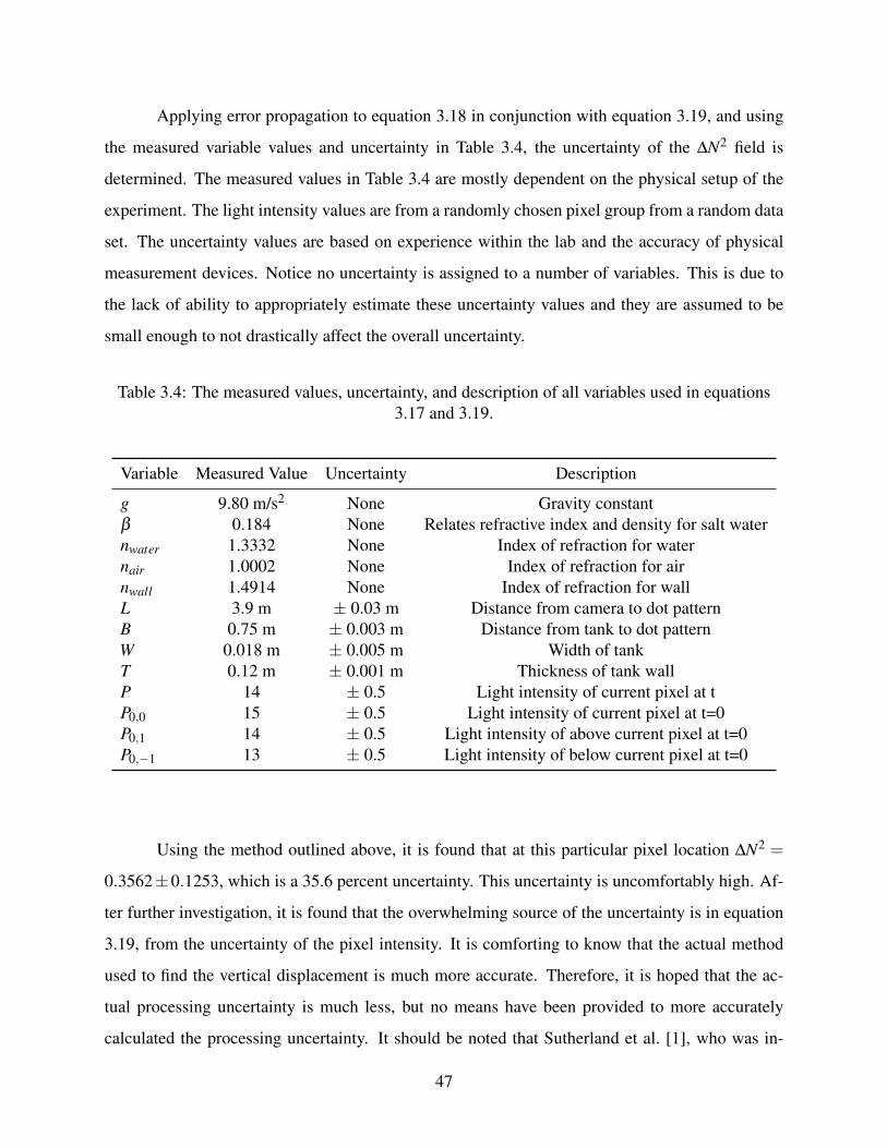
Applying error propagation to equation 3.18 in conjunction with equation 3.19, and using

the measured variable values and uncertainty in Table 3.4, the uncertainty of the ΔN2 field is

determined. The measured values in Table 3.4 are mostly dependent on the physical setup of the

experiment. The light intensity values are from a randomly chosen pixel group from a random data

set. The uncertainty values are based on experience within the lab and the accuracy of physical

measurement devices. Notice no uncertainty is assigned to a number of variables. This is due to

the lack of ability to appropriately estimate these uncertainty values and they are assumed to be

small enough to not drastically affect the overall uncertainty.

Table 3.4: The measured values, uncertainty, and description of all variables used in equations

3.17 and 3.19.

Variable Measured Value Uncertainty Description

g 9.80 m/s2 None Gravity constant

β 0.184 None Relates refractive index and density for salt water

nwater 1.3332 None Index of refraction for water

nair 1.0002 None Index of refraction for air

nwall 1.4914 None Index of refraction for wall

L 3.9 m ± 0.03 m Distance from camera to dot pattern

B 0.75 m ± 0.003 m Distance from tank to dot pattern

W 0.018 m ± 0.005 m Width of tank

T 0.12 m ± 0.001 m Thickness of tank wall

P 14 ± 0.5 Light intensity of current pixel at t

P0,0 15 ± 0.5 Light intensity of current pixel at t=0

P0,1 14 ± 0.5 Light intensity of above current pixel at t=0

P0,−1 13 ± 0.5 Light intensity of below current pixel at t=0

Using the method outlined above, it is found that at this particular pixel location ΔN2 =

0.3562±0.1253, which is a 35.6 percent uncertainty. This uncertainty is uncomfortably high. Af-

ter further investigation, it is found that the overwhelming source of the uncertainty is in equation

3.19, from the uncertainty of the pixel intensity. It is comforting to know that the actual method

used to find the vertical displacement is much more accurate. Therefore, it is hoped that the ac-

tual processing uncertainty is much less, but no means have been provided to more accurately

calculated the processing uncertainty. It should be noted that Sutherland et al. [1], who was in-

47

strumental in developing the synthetic schlieren method and who had a very similar experimental

setup, reported a uncertainty of around 5 percent.

A number of other factors are important in calculating the ΔN2 field, which were not in-

cluded in the above analysis, including: dot size, dot density, and thermal noise. The dot density

and size affect the interpolating algorithms used create a smooth ΔN2 field images from discrete

dot movements. Thermal noise is thought to be one of the largest factors in the uncertainty be-

cause it can drastically affect the refraction of light through air. Luckily, BYU’s stratified lab is

in an isolated location and does not have any major sources of thermal noise such as heating and

air conditioning. The only noticeable thermal source within the lab is the computer collecting the

data. In order to reduce the effects of this noise, a barrier is placed between the computer and the

line of sight of the camera. No noticeable thermal effects from the computer have been found with

this barrier in place.

3.5.2 Measurement Uncertainty Analysis

When forming the control volume around the interaction region, there is variability on

the precise location of the control volume. In other words, the control volume can be slightly

moved up, down, left, and right, and still contain the interaction region. This creates uncertainty

when measuring the energy crossing the control volume boundaries. In order to quantify this

uncertainty, the control volume around configuration 4, run 6, was moved five pixels up, down,

left, and right. Differences between the energy crossing the boundaries of the moved control

volume were compared with the energy crossing the boundaries of the original control volume.

Table 3.5 gives the percent change for the energy crossing the four boundaries one and

five pixels from the original control volume location in each direction. Boundaries one, two, and

four have little variation with the movement of the boundaries. Boundary three, where the primary

wave leaves, exhibits a greater uncertainty. This is likely due to the much smaller amount of energy

crossing this control volume when compared to the energy crossing boundaries one, two and four,

so any variation in energy will cause a larger percent change. Even though boundary three has

more variation than the other boundaries, it never changes by more than 3 percent, which is well

within reason.

48

Table 3.5: Percent change in the energy crossing the four boundaries of a control volume when

moved 1 and 5 pixels left, right, up, and down.

Boundary 1 Boundary 2 Boundary 3 Boundary 4

CV moved left 5 pixels -0.04 -0.14 -1.53 -0.10

CV moved left 1 pixel -0.01 -0.37 -0.30 -0.02

CV moved right 5 pixels -0.01 -0.74 1.41 0.10

CV moved right 1 pixel -0.04 -0.50 0.29 0.02

CV moved up 5 pixels 0.33 -2.77 -2.75 0.95

CV moved up 1 pixel 0.07 -0.83 -0.52 0.19

CV moved down 5 pixels -0.47 1.20 2.43 -0.84

CV moved down 1 pixel -0.08 -0.07 0.51 -0.18

From these results it can be concluded that measurement uncertainty from the positioning

of the control volumes is not a major source of uncertainty. In should be noted that any uncer-

tainty contained within the placement of the control volume is likely random and not systematic.

Therefore, the statistical uncertainty analysis will take into account the measurement uncertainty.

3.5.3 Statistical Uncertainty Analysis

As made apparent by the previous two sections, there is uncertainty in the experimental

results. This uncertainty can be classified in two categories: systematic or random. Systematic

uncertainty can be described as an offset or bias. It is where all the results are offset from the

actual values. Random uncertainty varies in repeated measurements. Random uncertainty causes

scatter in the results even when experimental conditions remain constant and is often impossible

to measure. Instead, a statistical analysis is used to approximate an actual value from repeated

measurements.

Statistical uncertainty analysis is based on three inputs: the spread or standard deviation of

the measured values (Sx), the confidence level (P), and the number of measured values (N). The

confidence level, usually 95%, is used in conjuction with the number of data points to find the t

value in the Student’s t distribution. The t value is then used to find the confident interval by

u =±tN−1,PSx (3.20)

49

where Sx is the standard deviation of the means found by Sx =Sx√

N.

At a 95% confidence level, the interval represented by u represents the numerical range

at which one can be 95% sure the actual value lies. In this study, statistical uncertainty analysis

is performed on the measurements of the energy partitioned to the harmonic frequencies. This

uncertainty will be represented as error bars in the results.

50

CHAPTER 4. RESULTS

Due to the nature of this study, there are a tremendous number of results that could be

shown. A total of eight configurations were analyzed; however, not all results for each configu-

ration need to be portrayed, largely due to their similarity. Any unique findings for a particular

configuration are explicitly shown. The results section is divided into qualitative and quantitative

results.

4.1 Qualitative Results

Figures 4.1 and 4.2 illustrate ΔN2 fields of the interaction for each configuration. Configu-

rations 1-4 are in Figure 4.1 and configurations 5-8 are in Figure 4.2 (recall that Figure 3.14 defines

the eight configurations). When looking at the interactions, it may helpful to recall how internal

waves propagate. As described more fully in section §1.3, the energy and phases of internal waves

propagate orthogonal to each other. The red and blue represent the phases of the internal waves

and can be thought of as crests and troughs. Dotted arrows show the direction the phases are prop-

agating, and solid arrows show the direction the energy is propagating or the direction the colliding

waves are approaching each other. Dashed lines show any harmonics generated by the interaction

that are visible without any filtering. However, the visualization of most harmonics requires the

images to be filtered. Notice harmonics are particularly visible in configurations 4 and 8. As will

be confirmed by the energy analysis, these two configurations create stronger harmonics than the

other configurations.

The filtered results for configurations 1-4 are found in Figures 4.3 and 4.4. These results

were found using the method described in §3.4.2 and have been filtered for the sum (| ω1 +ω2 |)and difference (| ω1−ω2 |) second-harmonic frequencies. All colormaps have been placed on the

same scale for easy magnitude comparison. Although the interaction can not be seen, the solid

lines represent the control volume surrounding the interaction region. Dashed lines show where

51

harmonics are seen propagating away from the interaction region and are predicted to be present

by Tabaei et al. [10]. In some cases, such as Figure 4.3(b), these waves are only visible at much

smaller scales and are not explicitly seen in these figures. The dotted lines are where harmonics

should be propagating from the interaction region according to Tabaei et al. but are not seen. This

can be caused by three possible explanations. One, harmonics do not exists at these locations.

Two, these harmonics are so small that they can not be resolved. Or finally, they are not seen due

to other disturbances in the fluid covering them up.

It is rather apparent from these figures that there are other disturbances at the second har-

monic frequencies. This is not completely unexpected. The wave beams created by the wave

generators are spatially finite. Therefore, despite being generated at a single frequency, these wave

beams must encapsule traces of other frequencies to create their finite structure. Also, it seems

that at the wave generation site, the harmonic frequencies are being excited to such an extent that

it appears that an actual wave at the harmonic frequency is being generated. An example of this

is seen in Figures 4.3(a) and 4.3(b). One of the wave generators is located just off the left of the

image between 0.1 and 0.2 meters on the ordinate. In both of these figures it appears the a wave

at each of the harmonic frequencies is being generated from this location. It is apparent that this

excitation is at the harmonic frequencies due to the angle at which these waves appear to be prop-

agating. Remember that internal wave propagation angle is directly dependent on the excitation

frequency (Equation 1.8). The fact that these disturbances are present will be an obstacle in the

energy analysis to follow.

Table 4.1 summarizes the comparison of the qualitative results with the predictions by

Tabaei et al. ‘No’ indicates where Tabaei et al. predicted harmonics to be present but were not seen.

‘Yes’ indicates a harmonic was predicted and seen. ‘–’ means that no harmonic was predicted. In

no case was a harmonic seen where Tabaei et al. did not predict a harmonic to be.

52

Meters

Met

ers

0.1 0.2 0.3 0.4 0.5 0.6 0.7 0.8 0.9

0.05

0.1

0.15

0.2

0.25

0.3

0.35

0.4

0.45

(a) Configuration 1

Meters

Met

ers

0.1 0.2 0.3 0.4 0.5 0.6

0.05

0.1

0.15

0.2

0.25

0.3

0.35

0.4

(b) Configuration 2

Meters

Met

ers

0.1 0.2 0.3 0.4 0.5 0.6 0.7 0.8 0.9

0.05

0.1

0.15

0.2

0.25

0.3

0.35

0.4

0.45

(c) Configuration 3

Meters

Met

ers

0.1 0.2 0.3 0.4 0.5 0.6

0.05

0.1

0.15

0.2

0.25

0.3

0.35

(d) Configuration 4

Figure 4.1: ΔN2 fields of the internal waves interacting for configuration 1-4. Solid arrows show the

direction the waves are approaching each other or the direction of energy propagation, and dotted

arrows show the direction of phase propagation. Dash lines represent any visible harmonics.

53

Meters

Met

ers

0.1 0.2 0.3 0.4 0.5

0.05

0.1

0.15

0.2

0.25

0.3

0.35

0.4

(a) Configuration 5

Meters

Met

ers

0.05 0.1 0.15 0.2 0.25 0.3 0.35 0.4 0.45

0.05

0.1

0.15

0.2

0.25

0.3

(b) Configuration 6

Meters

Met

ers

0.1 0.2 0.3 0.4 0.5

0.05

0.1

0.15

0.2

0.25

0.3

0.35

0.4

(c) Configuration 7

Meters

Met

ers

0.05 0.1 0.15 0.2 0.25 0.3 0.35 0.4 0.45

0.05

0.1

0.15

0.2

0.25

0.3

0.35

(d) Configuration 8

Figure 4.2: ΔN2 fields of the internal waves interacting for configuration 5-8. Solid arrows show the

direction the waves are approaching each other or the direction of energy propagation, and dotted

arrows show the direction of phase propagation. Dash lines represent any visible harmonics.

54

Meters

Met

ers

0.1 0.2 0.3 0.4 0.5 0.6 0.7 0.8 0.9

0.05

0.1

0.15

0.2

0.25

0.3

0.35

0.4

0.45

0.5

0.55

(a) Configuration 1, | ω1 +ω2 |

Meters

Met

ers

0.1 0.2 0.3 0.4 0.5 0.6 0.7 0.8 0.9

0.05

0.1

0.15

0.2

0.25

0.3

0.35

0.4

0.45

0.5

0.55

(b) Configuration 1, | ω1−ω2 |

Meters

Met

ers

0.1 0.2 0.3 0.4 0.5 0.6

0.05

0.1

0.15

0.2

0.25

0.3

0.35

0.4

(c) Configuration 2, | ω1 +ω2 |

Meters

Met

ers

0.1 0.2 0.3 0.4 0.5 0.6

0.05

0.1

0.15

0.2

0.25

0.3

0.35

0.4

(d) Configuration 2, | ω1−ω2 |

Figure 4.3: ΔN2 fields of the interaction filtered for the sum (|ω1+ω2 |) and difference (|ω1−ω2 |)second-harmonics for configurations 1 and 2. Solid lines are the control volumes surrounding the

interaction region. Dotted lines are locations where harmonics are expected but are not seen.

Dashed lines are where harmonics are expected and seen.

55

Meters

Met

ers

0.1 0.2 0.3 0.4 0.5 0.6 0.7 0.8 0.9

0.05

0.1

0.15

0.2

0.25

0.3

0.35

0.4

0.45

0.5

0.55

(a) Configuration 3, | ω1 +ω2 |

Meters

Met

ers

0.1 0.2 0.3 0.4 0.5 0.6 0.7 0.8 0.9

0.05

0.1

0.15

0.2

0.25

0.3

0.35

0.4

0.45

0.5

0.55

(b) Configuration 3, | ω1−ω2 |

Meters

Met

ers

0.1 0.2 0.3 0.4 0.5 0.6

0.05

0.1

0.15

0.2

0.25

0.3

0.35

0.4

0.45

(c) Configuration 4, | ω1 +ω2 |

Meters

Met

ers

0.1 0.2 0.3 0.4 0.5 0.6

0.05

0.1

0.15

0.2

0.25

0.3

0.35

0.4

0.45

(d) Configuration 4, | ω1−ω2 |

Figure 4.4: ΔN2 fields of the interaction filtered for the sum (|ω1+ω2 |) and difference (|ω1−ω2 |)second-harmonics for configurations 3 and 4. Solid lines are the control volumes surrounding the

interaction region. Dotted lines are locations where harmonics are expected but are not seen.

Dashed lines are where harmonics are expected and seen.

56

Table 4.1: Summary of whether a harmonic is seen propagating away from the interaction within

the two-dimensional quadrants, where the center of the interaction is at the origin. ‘ – ’ indicates

no harmonic is predicted to be present by Tabaei et al. [10].

Quadrant 1 Quadrant 2 Quadrant 3 Quadrant 4

Configuration 1

| ω1 +ω2 | No – – No

| ω1−ω2 | Yes No No No

Configuration 2

| ω1 +ω2 | No No No No

| ω1−ω2 | – No Yes –

Configuration 3

| ω1 +ω2 | – Yes No –

| ω1−ω2 | No Yes Yes No

Configuration 4

| ω1 +ω2 | Yes Yes No No

| ω1−ω2 | Yes – – Yes

Configuration 5

| ω1 +ω2 | No – – No

| ω1−ω2 | Yes No Yes No

Configuration 6

| ω1 +ω2 | No No No No

| ω1−ω2 | – No No –

Configuration 7

| ω1 +ω2 | – Yes No –

| ω1−ω2 | No Yes Yes No

Configuration 8

| ω1 +ω2 | Yes No No No

| ω1−ω2 | Yes – – Yes

57

4.2 Quantitative analysis

4.2.1 Harmonic Wavenumbers

In all waves, the wavenumbers are a critical component in defining the structure of the

waves. The wavenumbers are most easily visualized by creating a power spectrum of the flow

field. The power spectra of a lone primary and secondary wave for configuration 1 are found in

Figure 4.5. Power spectra are created by performing a two-dimensional Fourier transform on the

x-z flow field and show at which wavenumbers energy is concentrated. The white circle on the

power spectra represent the theoretical wavenumbers generated by the wave generator. Although

not perfect, the peaks of the power spectra are close to these points. One difficulty in using power

spectra to analyze a flow field is having enough resolution within the power spectra. This is ob-

viously an issue in these power spectra. The resolution of a power spectrum can only be refined

by increasing the size of the viewing window of the physical image captured, while maintaining

the same pixel-to-area resolution. In these power spectra, the viewing window is already near the

maximum for the lab setup.

k

m

−100 −50 0 50 100

−200

−150

−100

−50

0

50

100

150

200 0

0.2

0.4

0.6

0.8

1

1.2

1.4

1.6

(a) Primary Wave

k

m

−100 −50 0 50 100

−200

−150

−100

−50

0

50

100

150

200 0

1

2

3

4

5

(b) Secondary Wave

Figure 4.5: Power spectrum of the lone primary (a) and secondary (b) wave fields.

Figure 4.6 shows the power spectrum for the interaction of configuration 1. This power

spectrum has lines overlaying where energy within the primary (red), secondary (black), difference

harmonic (white), and sum harmonic (green) should lay along. These lines can be easy determined

58

due to the relationship between frequency and wavenumber in the dispersion relation (equation

1.9). The energy within the primary and secondary waves dominate this energy spectrum and no

energy within the harmonic frequencies can be seen. As a crude method to seeing if the interaction

truly is exciting the second-harmonics, the energy spectra of the lone primary and secondary waves

can be subtracted from the interaction energy spectrum. This results in the modified interaction

energy spectrum shown in Figure 4.7. The lines in this spectrum have the same meaning as those

in Figure 4.6. It is apparent that most of the energy within the primary and secondary waves is

now gone, especially in the secondary wave (along the black line). It is easy to see a concentration

of energy in the sum harmonic (green line). There is also energy that appears to coincide with the

difference harmonic (white line), although its proximity to the white and black lines makes this

argument questionable. These results would be more certain with greater resolution.

−200 −100 0 100 200

−200

−150

−100

−50

0

50

100

150

200 0

1

2

3

4

5

Figure 4.6: Power spectrum of the interaction for configuration 1. The lines are where energy

within the primary (red), secondary (black), difference harmonic (white), and sum harmonic

(green) should lay along.

59

−200 −100 0 100 200

−200

−150

−100

−50

0

50

100

150

200 0

0.05

0.1

0.15

0.2

0.25

0.3

0.35

Figure 4.7: Power spectrum of the interaction for configuration 1 with the power spectra for the

primary and secondary waves subtracted. The lines are where energy within the primary (red),

secondary (black), difference harmonic (white), and sum harmonic (green) should lay along.

The most effective method found to find the wavenumber for the generated harmonic is to

do a two-dimensional Fourier Transform on the already frequency filtered flow fields in 4.3 and

4.4. This resulted in power spectra that clearly showed the wavenumbers of the harmonics. This

process could only reasonably be done on filtered flow fields that were dominated by interaction

generated harmonics, not other disturbances. Therefore, configurations 3, 4, 7, and 8 are the only

candidates.

Following the Fourier Transform of these configurations, the horizontal and vertical wavenum-

bers with the greatest energy were recorded. Figure 4.8 shows these wavenumbers, as well as the

wavenumbers for the colliding waves. Figure 4.8(a) compares the wavenumber from configura-

tions 3 and 7. Recall that in these configurations, the colliding waves approach from the same

direction but at different angles. Configuration 7, which approaches at steeper angles than config-

uration 3, has higher horizontal wavenumbers in the colliding waves. The vertical wavenumbers

of the colliding waves are constant and constrained by the wave generators’ structure. As seen

60

in Figure 4.8(a), the harmonics resulting from the interaction in configuration 7 also have higher

horizontal harmonics and the vertical wavenumbers are relatively constant. A similar trend is seen

in Figure 4.8(b), between configurations 4 and 8. The main difference between the configurations

in Figure 4.8(a) and 4.8(b) is the slope between the given configuration’s harmonic wavenumbers.

Notice the slope between the harmonics for configurations 3 and 7 is positive, and the slope be-

tween the harmonics for configurations 4 and 8 is negative. This is likely due to the different

directions that the colliding waves are propagating when they collide.

0 20 40 60 80 1000

50

100

150

k

m

Config 3 colliding wavesConfig 7 colliding wavesConfig 3 harmonicsConfig 7 harmonics

(a)

0 20 40 60 80 1000

50

100

150

k

m

Config 4 colliding wavesConfig 8 colliding wavesConfig 4 harmonicsConfig 8 harmonics

(b)

Figure 4.8: Wavenumbers of colliding and second-harmonic waves for configuration 3 and 7 (a),

and 4 and 8 (b).

Unfortunately, more configurations with similar wave collision directions were not ana-

lyzed. An increase in configurations with similar wave collision directions may allow for a corre-

lation to be made between the colliding waves’ wavenumbers and their harmonics’ wavenumbers.

Such a correlation would be a large step in predicting the harmonics’ structure.

4.2.2 Energy Partition

As energy within the colliding waves enters the control volume, the energy will meet one of

two ultimate ends. It will be dissipated to the background by viscous forces within the interaction

region, or it will propagate out of the interaction within the colliding waves or harmonics. In order

to find either of these two outcomes, it is necessary to distinguish how much energy is entering

61

and leaving the control volume, and at what frequencies. Section §3.4.1 provides a method for

finding the energy within each frequency that crosses a control volume boundary. This enables

energy spectra to be formed depicting all the energy entering and exiting the control volume as

shown in Figure 4.9. The energy within the energy spectra is normalized by the total energy

entering the control volume and the frequency is normalized by the buoyancy frequency, ω =ω/N.

In these plots, the frequencies of the colliding waves are very apparent, and the energy within

these frequencies noticeably decreases from the time it enters the control volume to the time it

leaves. Also, on the outgoing energy spectrum there are two additional spikes around ω = 0.23

and 0.58 that represent the energy within the second harmonics. As expected, the frequencies of

the additional spikes are at the sum and difference of the colliding waves’ frequencies. These

energy spectra correspond to configuration 4. All other configurations have very similar incoming

and outgoing energy spectra.

0 0.2 0.4 0.6 0.8 10

0.1

0.2

0.3

0.4

0.5

0.6

0.7

Nor

mal

ized

Ene

rgy

Normalized Frequency

(a) Incoming Energy

0 0.2 0.4 0.6 0.8 10

0.1

0.2

0.3

0.4

0.5

0.6

0.7

Nor

mal

ized

Ene

rgy

Normalized Frequency

(b) Outgoing Energy

Figure 4.9: Energy spectrums of incoming (a) and outgoing (b) energy for configuration 4.

Energy Remaining in Colliding Waves

By knowing the energy at each frequency and whether the energy is entering or leaving

the control volume, the energy within each wave can be determined. Figure 4.10 illustrates the

energy within the primary and secondary waves entering and leaving the control volume for all 16

runs of configuration 1. The energy is again normalized by the total energy entering the interaction.

62

These plots provide the ability to compare all the runs simultaneously, and show that energy within

each wave is fairly consistent for all runs. Also, it is easily seen how much energy remains in the

colliding waves after the interaction. Although not shown, the results for all configuration are

similar.

0 5 10 150

0.2

0.4

0.6

0.8

1Primary Wave Energy In

Nor

mal

ized

Ene

rgy

0 5 10 15

Secondary Wave Energy In

0 5 10 150

0.2

0.4

0.6

0.8

1Primary Wave Energy Out

Run

Nor

mal

ized

Ene

rgy

0 5 10 15

Secondary Wave Energy Out

Run

Figure 4.10: Energy within the primary and secondary waves as they enter and leave the control

volume for all 16 runs of configuration 1.

Energy Partitioned to Harmonics

One of the main objectives in this study is to find how much energy is partitioned to the

second-harmonic. Figures 4.11 and 4.12 provide these results for each run in each configuration.

The results are again normalized by the total energy entering the interaction for each run. Each

configuration’s results distinguish between the energy partitioned to the sum second-harmonic

63

(ω1 +ω2) and the difference second-harmonic (ω1−ω2). Generally, the results are fairly con-

sistent; although, it does not take much to find a few anomalies. These outliers may be caused by

any number of uncertainties within the experiment. If any data point is outside the 95% percent

confidence interval as determined by all the points in the given run, then this point was thrown out

of any further results. The upper and lower bounds of this confidence interval are shown by the

dash lines.

0 100

0.01

0.02

0.03

0.04

0.05

0.06

0.07

0.08ω1+ω2

Run

Nor

mal

ize

Ene

rgy

(Eha

rmon

ic/E

tota

l)

0 10

ω1−ω2

Run

(a) Configuration 1

0 5 10 150

0.01

0.02

0.03

0.04

0.05

0.06

0.07

0.08ω1+ω2

Run

Nor

mal

ize

Ene

rgy

(Eha

rmon

ic/E

tota

l)

0 5 10 15

ω1−ω2

Run

(b) Configuration 2

0 10 200

0.01

0.02

0.03

0.04

0.05

0.06

0.07

0.08ω1+ω2

Run

Nor

mal

ize

Ene

rgy

(Eha

rmon

ic/E

tota

l)

0 10 20

ω1−ω2

Run

(c) Configuration 3

0 100

0.01

0.02

0.03

0.04

0.05

0.06

0.07

0.08ω1+ω2

Run

Nor

mal

ize

Ene

rgy

(Eha

rmon

ic/E

tota

l)

0 10

ω1−ω2

Run

(d) Configuration 4

Figure 4.11: Energy, normalized by the total energy entering the interaction, within the sum

second-harmonic (| ω1 +ω2 |) and the difference second-harmonic (| ω1−ω2 |) for each exper-

imental run. Dashed lines are the upper and lower bounds for the 95% confidence interval. Figure

includes configurations 1-4.

64

0 100

0.01

0.02

0.03

0.04

0.05

0.06

0.07

0.08ω1+ω2

Run

Nor

mal

ize

Ene

rgy

(Eha

rmon

ic/E

tota

l)

0 10

ω1−ω2

Run

(a) Configuration 5

0 10 200

0.01

0.02

0.03

0.04

0.05

0.06

0.07

0.08ω1+ω2

Run

Nor

mal

ize

Ene

rgy

(Eha

rmon

ic/E

tota

l)

0 10 20

ω1−ω2

Run

(b) Configuration 6

0 10 200

0.02

0.04

0.06

0.08

0.1ω1+ω2

Run

Nor

mal

ize

Ene

rgy

(Eha

rmon

ic/E

tota

l)

0 10 20

ω1−ω2

Run

(c) Configuration 7

0 10 200

0.01

0.02

0.03

0.04

0.05

0.06

0.07

0.08ω1+ω2

Run

Nor

mal

ize

Ene

rgy

(Eha

rmon

ic/E

tota

l)

0 10 20

ω1−ω2

Run

(d) Configuration 8

Figure 4.12: Energy, normalized by the total energy entering the interaction, within the sum

second-harmonic (ω1 +ω2) and the difference second-harmonic (ω1−ω2) for each experimen-

tal run. Dashed lines are the upper and lower bounds for the 95% confidence interval. Figure

includes configurations 5-8.

Notice that some configurations have more runs than others. If a configuration conveyed

an unusual trend within the first 15 runs, more runs were taken in order to dispel or confirm these

trends. Take the difference harmonic in configuration 6 for example (Figure 4.12(b)). In the initial

15 runs, there seemed to be a consistent decrease of energy within this harmonic. It was unsure

whether the first runs were unusually high, or the latter runs were unusually low, or some proce-

dural change caused energy to appear to decrease with each run. After completing six additional

65

experiments, it was easily seen that the apparent decrease was nothing more than coincidence, and

all experiments seemed to surround a common value.

The results in Figures 4.11 and 4.12 can be summarized in two plots as illustrated in Figure

4.13 for the two harmonics. The error bars represent the 95% confidence interval of the means.

This confidence interval is different than the interval used in the previous plots and represents the

interval that contains the actual value as described in section §3.5.

These plots display an interesting pattern. Notice that the trend of the energy partitioned

in configurations 1-4 is repeated for configuration 5-8. Recall that the only difference between

configurations 1-4 and 5-6 is the angle at which the waves approach each other. In other words,

in configuration 1 and 5 the primary and secondary waves approach from the same direction but

at different angles. Same with configuration 2 and 6, and so forth. By noticing this repeated trend

between configurations 1-4 and 5-8, it becomes clear that the direction from which the waves ap-

proach is more important to how much energy is partitioned to the harmonics, than the actual angle

at which the waves approach. From this trend, it would not be difficult to predict an approximate

value of energy dispersed to the second-harmonics of any other two waves colliding from similar

directions.

The difference harmonic has relatively little energy partitioned to it for all of the config-

urations. Configurations 4 and 8 partition the most energy to this harmonic at around 2%. The

sum harmonic has a much larger amount of energy partitioned to it for configurations 3, 4, 7, and

8. Notice that all these configurations have one wave colliding from the top of the interaction and

one wave colliding from the bottom. This leads to the conclusion that a larger amount of energy

is partitioned to the sum second-harmonic when the colliding waves have opposite signed vertical

wavenumbers.

This study focuses only on the second-harmonic, which is usually the strongest harmonic

excited by the interaction. However, in reality each interaction produces a myriad of harmonics,

all at the sum and difference of multiples of the colliding waves’ frequencies, according to equa-

tion 1.3. Despite each interaction exciting many harmonic frequencies, no interaction produced a

noticeable spike in the outgoing energy spectrum at any additional harmonic frequency with the

exception of configurations 4 and 8. Interestingly, these interactions generated a relatively strong

third-harmonic at a frequency of | 2ω1 +ω2 |. The energy partitioned to this harmonic is found

66

0 2 4 6 80

0.01

0.02

0.03

0.04

0.05

0.06

0.07

0.08

Configuration

Nor

mal

ized

Ene

rgy

(a) (ω1 +ω2)

0 2 4 6 80

0.01

0.02

0.03

0.04

0.05

0.06

0.07

0.08

Configuration

Nor

mal

ized

Ene

rgy

(b) (ω1−ω2)

Figure 4.13: Normalized energy partitioned to the sum harmonic (a) and difference harmonic (b).

Error bars represent the statistical 95% confidence interval of the mean.

in Figure 4.14. The presence of this harmonic reaffirms how dependent the response of internal

waves colliding is on the direction from which the waves collide. This harmonic is nearly equal in

strength to the difference second-harmonic, although it is obvious that configuration 8 partitions

more energy to this harmonic. Tabaei et al. [10] also found some higher-order harmonics of equal

or even greater strength than lower-order harmonics.

0 5 10 150

0.01

0.02

0.03

0.04

0.05

0.06

0.07

0.08

Run

Nor

mal

ized

Ene

rgy

(a) Configuration 4

0 5 10 15 200

0.01

0.02

0.03

0.04

0.05

0.06

0.07

0.08

Run

Nor

mal

ized

Ene

rgy

(b) Configuration 8

Figure 4.14: Energy partitioned to a third-harmonic, | 2ω1+ω2 |, in configurations 4 (a) and 8 (b).

67

Adjusted Energy Partitioned to Harmonics

When filtering for the harmonic frequencies from the wave fields, it was found that the

primary and secondary waves contained traces of the harmonic frequencies. The presence of this

energy invariably effects how much energy is perceived to be partitioned to the harmonic frequen-

cies. This begs the question, how much energy found within the harmonic frequencies is a result

of the finite structure of the primary and secondary waves? Although there is no perfect way to

find the answer to this question, there are means to predict the answer.

To illustrate how this problem is solved consider Figure 4.15(a), which shows the energy

spectrum for a plane where a secondary wave leaves the control volume. The most energy is

concentrated at approximately ω = 0.4, the frequency of the secondary wave, and exponentially

decreased on either side. It is obvious that the energy from the secondary wave has not decayed to

zero before reaching the harmonic frequencies at approximately ω = 0.22 and 0.57. This further

demonstrates the fact that the secondary wave, and similarly the primary wave, is contributing to

the energy found within the harmonics.

0 0.2 0.4 0.6 0.8 10

0.05

0.1

0.15

0.2

0.25

Normalized Frequency

Nor

mal

ized

Ene

rgy

(a) Configuration 4

0.1 0.2 0.3 0.4 0.5 0.6 0.70

0.02

0.04

0.06

0.08

0.1

Normalized Frequency

Nor

mal

ized

Ene

rgy

(b) Configuration 8

Figure 4.15: Energy spectrum for the secondary wave leaving the control volume for configuration

4. The presents of the secondary wave contributes to the energy found in the harmonic normalized

frequencies, ω = 0.22 and 0.57. Figure (b) is a zoomed up representation of (a) with a curve fit

formed from the ‘x’ marker points.

To estimate the energy contributed to the harmonics from the colliding waves, an exponen-

tial curve fit is created along the decaying energy before the harmonic frequencies. Figure 4.15(b)

68

demonstrates how this curve fit can be formed from 3 points as indicated by the ‘x’ marker. This

figure is a zoomed in version of Figure 4.15(a). The curve fit is performed on both sides of the

decaying energy spectrum. Other curves fit were attempted, including a Gaussian and exponential

curve fit including the peak points. Both of these curve fits had much larger residuals than the

simple curve shown in the figure. This curve fit is then used to estimate how much energy within

the harmonic frequency is present as a results of the secondary wave. In this case, a relatively sub-

stantial portion of the energy within the ω = 0.57 harmonic is due to the secondary wave compared

to the ω = 0.22 harmonic. A similar curve fit can be formed from the primary wave and at all four

control volume borders. The resulting energy from the curve fit at the harmonic frequencies is then

subtracted from the energy found at those frequencies. This results in an adjusted energy partition

to the harmonics that should more accurately represent the energy partitioned to the harmonics as

a result of the interaction. Figure 4.16 shows the results after excluding outliers and finding the

95% confidence interval of the means. The results are on average 10% lower than those previously

found. The larges change happened to the difference second-harmonic in configuration 2, which

lowered by 25%. The difference second-harmonic in configuration 7 lowered the least, at 1%.

0 2 4 6 8 100

0.01

0.02

0.03

0.04

0.05

0.06

0.07

0.08

Configuration

Nor

mal

ized

Ene

rgy

(a) (ω1 +ω2)

0 2 4 6 80

0.01

0.02

0.03

0.04

0.05

0.06

0.07

0.08

Configuration

Nor

mal

ized

Ene

rgy

(b) (ω1−ω2)

Figure 4.16: Adjusted energy partitioned to the sum harmonic (a) and difference harmonic (b).

Error bars represent the statistical 95% confidence interval of the mean.

The overall harmonic energy partition conclusion discussed before are still valid after the

adjustments. There is still a general repeating trend between configurations 1-4 and 5-8, and a great

deal more energy is partitioned to the sum harmonic for configurations where the secondary wave

69

is approach the interaction from the opposite vertical direction than the primary wave. However,

these adjusted results should be more accurate.

Energy Dissipated

By extending the energy analysis one step further, the energy lost to viscous dissipation

can be found. As seen previously, all the energy entering and exiting the interaction has been

accounted for. By taking the difference of the energy entering and leaving the control volume,

an estimation for the energy dissipated results. Using the average energy leaving in each colliding

wave, partitioned to the second harmonic, and dissipated, a bar plot representing the outcome of all

energy entering the interaction is created as shown in Figure 4.17. The interaction region for each

configuration is not the same; therefore, some interactions lose a great deal more energy to viscous

dissipation. This is made clear in configurations 1, 3, 5, and 7, which have the largest interaction

regions.

The large amount of energy shown dissipated in the bar plot may seem alarmingly high.

These amounts were corroborated by finding the amount of energy dissipated by individual waves

propagating through the control volumes used around the configurations. These results show a

similar amount of energy being dissipated over the same region.

Any energy that did not leave the interaction in one of the colliding waves or second-

harmonics, or get dissipated, is referred to as energy with an unknown outcome. The most plausible

theory for the outcome of this energy is it is dispersed to other higher-order harmonics, such as

those found in configurations 4 and 8. It is even possible that energy is dispersed to harmonics that

would cause evanescent waves. This frequency range was not explored in this study, so this remains

only as a possible outcome of this energy. Javam et al. [8], Teoh et all. [7], and Chashechkin and

Neklyudov [6] all found evanescent frequencies excited in their colliding internal wave studies.

The energy with unknown outcome stays fairly consistent for all configuration from 5 to 8 percent.

Overall, the majority of the energy entering the interaction is either dissipated within the

interaction region or exits the interaction within the colliding waves. Only 2 to 8 percent of the

energy is partitioned to one of the second harmonics, with configuration 3, 4, 7, and 8 partitioning

the most. This leaves the remaining 5 to 8 percent of the energy being partitioned to all other

higher-order harmonics.

70

1 2 3 4 5 6 7 80

20

40

60

80

100

Configuration

Per

cent

of E

nerg

y E

nter

ing

Inte

ract

ion

Energy with unknown outcomeEnergy partitioned to harmonicsEnergy leaving in colliding wavesEnergy dissipated

Figure 4.17: Estimated outcome of all energy entering the interaction.

71

CHAPTER 5. CONCLUSIONS

Internal waves are ubiquitous phenomena that occur in both the atmosphere and ocean. As

they propagate, they may encounter a myriad of other fluid phenomena, including other internal

waves. Internal waves interactions may be classified in one of two categories: resonant and non-

resonant. Non-resonant interactions, the focus of this research, have not been a major focus in

previous research. When two non-resonant internal waves collide, harmonics are formed at the

sum and difference of multiples of the colliding waves’ frequencies. The goal of this study is

to visualize the flow field, compare qualitative results to Tabaei et al., and determine the energy

partition to the second-harmonic for two interacting non-resonant internal waves at eight unique

configurations.

In order to create a wave-wave interaction, two identical wave generators were designed.

Although not perfect, the wave generators create temporally and spatially monochromatic waves

that have vertical and horizontal wavenumbers reasonable close to the user’s specifications. The

lab is setup to provide as accurate results as possible and procedures are standardized to limit

variability. Results from the lab are proven to be both accurate and repeatable.

When the interaction results are compared with predictions by Tabaei et al., not all the

expected harmonic waves can be seen. This, however, does not necessarily mean that the har-

monics do not exist. Other harmonic frequency disturbances may be masking the presences of the

harmonics. No harmonics were seen where they were unexpected. The wavenumbers of the har-

monics seem to have a direct correlation to the wavenumbers of the colliding waves. An increase in

the horizontal wavenumbers of the colliding waves leads to an increase in the second-harmonics’

horizontal wavenumbers.

An energy analysis is also performed to find the energy partitioned to the second-harmonic.

The original results must be adjusted due to other harmonic frequency disturbances causing a bias.

An exponential curve is is used to estimate the extent of this bias for each run. The adjusted results

73

lower the original results by an average of 10 percent. It is found that between 0.5 and 7 percent of

the colliding waves’ energy is partioned to the second-harmonics, depending on the configuration.

This energy analysis indicates that the relative direction in which the colliding waves approach

each other has much more of an effect on the partition of energy to the second-harmonic than

the angles at which the colliding waves propagate. These results are compelling enough that a

reasonable estimation of the energy partitioned to second-harmonics could be approximated for

similar configurations. It is also found that when internal waves that have opposite signed vertical

wavenumbers collide, a much larger amount of energy to the sum second-harmonic.

When energy within the colliding waves enters the interaction region, very little of the

energy is actually partitioned to harmonics. Most of the energy is dissipated by viscous forces or

leaves the interaction within the colliding waves. For configurations 1, 3, 5, and 7, approximatly

50 percent of the energy entering the interaction is dissipated. The remaining configurations lost

around 30 percent to dissipation. These configurations lost less energy to dissipation becuase of

their smaller interaction region. For all eight configurations studied, 5 to 8 percent of the energy

entering the interaction has an unknown fate. It is hypothesized that this energy is likely partitioned

to higher-order harmonics. For configurations 4 and 8, it is seen that a relatively large amount of

energy is partitioned to the higher-order, third-harmonic, between 1 to 3 percent.

5.1 Contributions

The following list enumerates the unique contributions made by this research to the scien-

tific community.

• A novel method to analyze energy entering and exiting a control volume when studying

internal waves.

• The visualization of the complete flow field for a variety of internal wave nonresonant inter-

actions.

• An estimate of the energy partitioned to the second-harmonic for nonresonant interactions

within the two-dimensional plane.

74

• Understanding that the energy partition to the second-harmonics is much more dependent on

the colliding wave’s direction that angle.

• Support, but not verification, of the theory presented by Tabaei et al.

5.2 Future Work

There are a number of directions this research can take. One of the most natural directions

it can take is to continue the comparison between laboratory results and predictions by Tabaei et

al., but now compare quantitative results. This work can also be easily extended by analyzing

additional harmonic frequencies, including evanescent frequencies. There may be some other

harmonic that has been partitioned a substantial amount of energy.

The wavenumber analysis opened up another door that could be explored. Additional inter-

action configurations could be studied with waves colliding from similar directions while changing

the vertical and horizontal wavenumbers independently. Relating the resulting colliding waves’

wavenumber and the harmonics’ wavenumber could lead to a correlation. Therefore, the wave

structure of harmonics could be predicted by the wave structure of the colliding waves.

Additional work could also be done by extending the collision configurations into the third

dimension. Also, the transient startup of colliding waves could be analyzed.

75

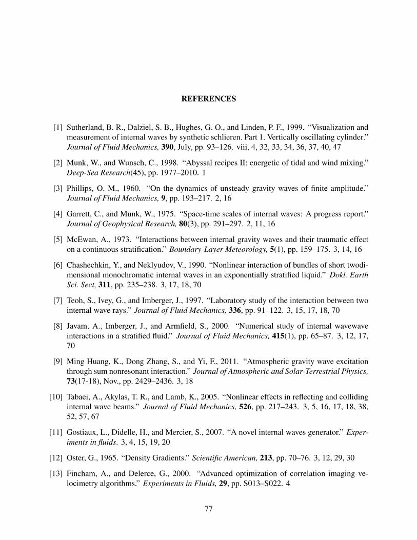
REFERENCES

[1] Sutherland, B. R., Dalziel, S. B., Hughes, G. O., and Linden, P. F., 1999. “Visualization and

measurement of internal waves by synthetic schlieren. Part 1. Vertically oscillating cylinder.”

Journal of Fluid Mechanics, 390, July, pp. 93–126. viii, 4, 32, 33, 34, 36, 37, 40, 47

[2] Munk, W., and Wunsch, C., 1998. “Abyssal recipes II: energetic of tidal and wind mixing.”

Deep-Sea Research(45), pp. 1977–2010. 1

[3] Phillips, O. M., 1960. “On the dynamics of unsteady gravity waves of finite amplitude.”

Journal of Fluid Mechanics, 9, pp. 193–217. 2, 16

[4] Garrett, C., and Munk, W., 1975. “Space-time scales of internal waves: A progress report.”

Journal of Geophysical Research, 80(3), pp. 291–297. 2, 11, 16

[5] McEwan, A., 1973. “Interactions between internal gravity waves and their traumatic effect

on a continuous stratification.” Boundary-Layer Meteorology, 5(1), pp. 159–175. 3, 14, 16

[6] Chashechkin, Y., and Neklyudov, V., 1990. “Nonlinear interaction of bundles of short twodi-

mensional monochromatic internal waves in an exponentially stratified liquid.” Dokl. EarthSci. Sect, 311, pp. 235–238. 3, 17, 18, 70

[7] Teoh, S., Ivey, G., and Imberger, J., 1997. “Laboratory study of the interaction between two

internal wave rays.” Journal of Fluid Mechanics, 336, pp. 91–122. 3, 15, 17, 18, 70

[8] Javam, A., Imberger, J., and Armfield, S., 2000. “Numerical study of internal wavewave

interactions in a stratified fluid.” Journal of Fluid Mechanics, 415(1), pp. 65–87. 3, 12, 17,

70

[9] Ming Huang, K., Dong Zhang, S., and Yi, F., 2011. “Atmospheric gravity wave excitation

through sum nonresonant interaction.” Journal of Atmospheric and Solar-Terrestrial Physics,73(17-18), Nov., pp. 2429–2436. 3, 18

[10] Tabaei, A., Akylas, T. R., and Lamb, K., 2005. “Nonlinear effects in reflecting and colliding

internal wave beams.” Journal of Fluid Mechanics, 526, pp. 217–243. 3, 5, 16, 17, 18, 38,

52, 57, 67

[11] Gostiaux, L., Didelle, H., and Mercier, S., 2007. “A novel internal waves generator.” Exper-iments in fluids. 3, 4, 15, 19, 20

[12] Oster, G., 1965. “Density Gradients.” Scientific American, 213, pp. 70–76. 3, 12, 29, 30

[13] Fincham, A., and Delerce, G., 2000. “Advanced optimization of correlation imaging ve-

locimetry algorithms.” Experiments in Fluids, 29, pp. S013–S022. 4

77

[14] Dalziel, S. B., Hughes, G. O., and Sutherland, B. R., 2000. “Whole-field density measure-

ments by ’synthetic schlieren’.” Experiments in Fluids, 28(4), Apr., pp. 322–335. 4, 13,

32

[15] Sutherland, B. R., 2010. Internal Gravity Waves. 6, 7, 9

[16] Staquet, C., and Sommeria, J., 2002. “Internal Gravity Waves: From Instabilities to Turbu-

lence.” Annual Review of Fluid Mechanics, 34, pp. 559–593. 11

[17] Briscoe, M. G., 1975. “Internal waves in the ocean.” Reviews of Geophysics and SpacePhysics, 13, pp. 591–598. 11

[18] Munk, W. H., 1981. “A survey of internal waves and small-scale processes.” Evolution ofPhysical Oceanography, pp. 264–291. 11, 16

[19] Rattray, M., 1960. “On the Coastal Generation of Internal Tides.” Tellus, 12(1), pp. 54–62.

11

[20] Baines, P. G., 1974. “The Generation of Interanl Tide over Steep Continental Slopes.” Phili-sophical Transactions of the Royal Society of London, 277(1263), pp. 27–58. 11

[21] Lee, C.-Y., and Beardsley, R. C., 1974. “The Generation of Long Nonlinear Internal Waves

in a Weakly Stratified Shear Flow.” Journal of Geophysical Research, 79(3), pp. 453–462.

11

[22] Hibiya, T., 1986. “Generation Mechanism of Internal Waves by Tidal Flow Over a Sill.”

Journal of Geophysical Research, 91(6), pp. 7697–7708. 11

[23] Bell, T. H., 1975. “Topographically Generated Internal Waves in the Open Ocean.” Journalof Geophysical Research, 80(3), p. 320. 11

[24] Rudnick, D. L., 2003. “From Tides to Mixing Along the Hawaiian Ridge.” Science,301(5631), July, pp. 355–357. 11

[25] Merrifield, M. a., Holloway, P. E., and Johnston, T. M. S., 2001. “The generation of internal

tides at the Hawaiian Ridge.” Geophysical Research Letters, 28(4), p. 559. 11

[26] Helfrich, K. R., and Melville, W. K., 2006. “Long Nonlinear Internal Waves.” Annual Reviewof Fluid Mechanics, 38(1), Jan., pp. 395–425. 11, 12

[27] Baines, P., 1985. “Stratified Flow over Two-Dimensional Topography in Fluid of Infinite

Depth: A Laboratory Simulation.” Journal of the atmospheric sciences, 42(15), pp. 1614–

1630. 11, 14, 29

[28] Mowbray, D. E., and Rarity, D. S. H., 1967. “A theoretical and experimental investigation

of the phase configuration of internal waves of small amplitude in a density stratified liquid.”

Journal of Fluid Mechanics1, 28(1), pp. 1–16. 11, 14

[29] Broutman, D., Rottman, J. W., and Eckermann, S. D., 2004. “Ray Methods for Internal Waves

in the Atmosphere and Ocean.” Annual Review of Fluid Mechanics, 36(1), Jan., pp. 233–253.

12

78

[30] Helfrich, K. R., and Melville, W. K., 2006. “Long Nonlinear Internal Waves.” Annual Reviewof Fluid Mechanics, 38(1), Jan., pp. 395–425. 12

[31] Muller, P., Holloway, G., Henyey, F., and Pomphrey, N., 1986. “Nonlinear Interactions

Among Internal Gravity Waves.” Reviews of Geophysics, 24(3), pp. 493–536. 12, 16

[32] Economidou, M., and Hunt, G. R., 2008. “Density stratified environments: the double-tank

method.” Experiments in Fluids, 46(3), Oct., pp. 453–466. 13, 30

[33] Hill, D. F., 2002. “General density gradients in general domains : the two-tank method

revisited.” Experiments in Fluids, 32, pp. 434–440. 13, 30

[34] Peacock, T., and Echeverri, P., 2008. “An Experimental Investigation of Internal Tide Genera-

tion by Two-Dimensional Topography.” Journal of Physical Oceanography, 38, pp. 235–242.

14, 34

[35] Zhang, H. P., King, B., and Swinney, H. L., 2007. “Experimental study of internal gravity

waves generated by supercritical topography.” Physics of Fluids, 19(9), p. 096602. 14, 34

[36] Garrett, C., and Kunze, E., 2007. “Internal Tide Generation in the Deep Ocean.” AnnualReview of Fluid Mechanics, 39, pp. 57–87. 14

[37] Fritts, D. C., and Alexander, M. J., 2003. “Gravity wave dynamics and effects in the middle

atmosphere.” Reviews of Geophysics, 41(1), pp. 1–64. 14

[38] Sutherland, Bruce R.; Linden, P., 1998. “Internal wave excitation from stratified flow over a

thin barrier.” Journal of Fluid Mechanics, 377, pp. 223–252. 14, 29

[39] Aguilar, D. A., Sutherland, B. R., and Muraki, D. J., 2006. “Laboratory generation of internal

waves from sinusoidal topography.” Deep-Sea Research, 53, pp. 96–115. 14, 29, 34

[40] Echeverri, P., Flynn, M. R., Winters, K., and Peacock, T., 2009. “Low-mode internal tide

generation by topography : an experimental and numerical investigation Accessed.” Journalof Fluid Mechanics, 636, pp. 91–108. 14, 34

[41] Anson, J., and Sutherland, B. R., 2010. “Internal gravity waves generated by convective

plumes.” Journal of Fluid Mechanics, 648, pp. 405–434. 14

[42] Flynn, M. R., and Sutherland, B. R., 2004. “Intrusive gravity currents and internal gravity

wave generation in stratified fluid.” Journal of Fluid Mechanics, 514, pp. 355–383. 14, 34

[43] Dauxois, T., Didier, A., and Falcon, E., 2004. “Observation of near-critical reflection of

internal waves in a stably stratified fluid.” Physics of Fluids, 16, p. 1936. 14

[44] Peacock, T., and Tabaei, A., 2005. “Visualization of nonlinear effects in reflecting internal

wave beams.” Physics of Fluids, 17(6), p. 061702. 15

[45] Gostiaux, L., Dauxois, T., Didelle, H., and Sommeria, J., 2006. “Quantitative laboratory

observations of internal wave reflection on ascending slopes.” Physics of Fluids. 15

[46] Mercier, M., Martanand, D., Mathur, M., Gostiaux, L., Peacock, T., and Dauxois, T., 2010.

“New wave generation.” Journal of Fluid Mechanics, 657, pp. 308–334. 15, 19, 20, 25

79

[47] Mathur, M., and Peacock, T., 2009. “Internal wave beam propagation in non-uniform strati-

fications.” Journal of Fluid Mechanics, 639, pp. 133–152. 15

[48] Godoy-Diana, R., Chomaz, J.-M., and Donnadieu, C., 2006. “Internal gravity waves in a

dipolar wind: a wavevortex interaction experiment in a stratified fluid.” Journal of FluidMechanics, 548, Feb., pp. 281–308. 15

[49] Blackhurst, T., 2012. “Numerical Investigation of Internal wave-vortex interactions.” Mas-

ter’s thesis, Brigham Young University. 15

[50] Rodenborn, B., Kiefer, D., Zhang, H. P., and Swinney, H. L., 2011. “Harmonic generation by

reflecting internal waves.” Physics of Fluids, 23. 16, 26

[51] Thorpe, S., and Haines, A., 1987. “On the reflection of a train of finite-amplitude internal

waves from a uniform slope.” Journal of Fluid Mechanics, 178, Apr., pp. 279–302. 16

[52] McComas, H., and Bretherton, F., 1977. “Resonant Interaction of Oceanic Internal Waves.”

Journal of Geophysical Research, 82(9). 16

[53] Lvov, Y., Polzin, K., and Yokyama, N., 2007. “Resonant and Near-Resonant Internal Wave

Interactions.” Arxiv preprint arXiv:0706.3712. 16

[54] Martin, S., Simmons, W. F., and Wunsck, C. I., 1969. “Resonant internal wave interactions.”

Nature, 224, pp. 1014–1016. 16

[55] Sutherland, B. R., and Linden, P. F., 2002. “Internal wave excitation by a vertically oscillating

elliptical cylinder.” Physics of Fluids, 14(2), p. 721. 29

[56] Burton, R., 1949. “A modified schlieren apparatus for large areas of field.” Journal of theOptical Society of America, 39, pp. 907–909. 32

80

APPENDIX A. WAVE GENERATOR DRAWING PACKAGE

The following pages contain the drawing package for the wave generator designed in this

study.

81

82

83

6,000

1,750

5,500

1,000

4,500

4,0

00

0,2

50

3,7

50

0,1

00

0,3

00

0,125

0,325

0,1

00

0,3

00

1,000

4,500 0

.05 X

3

TA

P 6

-32

0.5

X 4

2,5

2,0

C A

4

2

B

3

D

3

C

B

A

4

1/5

/2012

5

1

6

Inches

Alu

min

um

56

D

To

p C

asin

g P

late

21

0,2

84

0,100

0,300

4,0

00

1,000

4,500

0,500

1,500

2,750

3,750

6,000

0,0

96

0,2

96

0,5

00

0,6

00

0,2

50

0.0

625 X

4

0,2

50

3,7

50

0.0

2 X

4

5,5

2,0

1,5

TA

P 6

-3

2

0.5

X 6

B

Alu

min

um

112

33

44

55

66

AA

BCC

DD

2

1/5

/2012

Bo

tto

m C

asin

g P

late

Inches

85

4,4

0

0,9

0

1,0

0

1,50

0,2

5

3,4

0

3,5

0

0,5

0

3,4

0

0,50

1,50

3,50

4,50

6,00

0.0

625 X

4

0,5

2,9

C A

4

2

B

3

D

3

C

B

A

4

1/5

/2012

5

1

6

Inches

Acrylic

56

D

Pla

te

21

86

35

,50

0

2,7

50

0,250

0,2

00

0,075

1

43

5

1/5

/2012

3

D

CC

Alu

min

um

6

5

AD

1

4

Sh

aft

B

6

2

B

2

Inches

A

87

1,5

00

0,0

75

0,2

00

0,3

94

0.2

50 *

See N

ote

1/5

/2012

D

4

25

1 1

C

4

Inches

6

B

Ca

ms

2

Acrylic

AA

3

B

53

D C

6

Note

: S

haft h

ole

is s

em

icircula

r w

/ specifie

d g

eom

etr

y.

Each s

haft h

ole

is r

ota

ted e

xactly 4

5 d

egrees from

previo

us c

am

.

88

89

90

APPENDIX B. LAB PROCEDURES

The following pages contain lab procedures for the filling and emptying the tank, and taking

density measurement to determine the stratification.

91

Emptying the Tank or Barrels Diagram of Setup

1. Place the end of the hose in the Tank/Barrels. (Image 1)

2. Make sure the open end of the “T” on the hose is securely directed into the black drain pipe (you may need to hold it there for the duration of emptying the tank). Note: If the hose isn’t secure, it will likely come out of the drain pipe and shoot water everywhere.

3. Turn the knob on the “T” of the hose to be parallel with the open end. This opens the valve so water will come out of the “T”. (Image 2)

4. Turn the water on. Water will now flow out the open end of the “T”. A low pressure is created within the flow of the hose which essentially creates a siphon that will now empty the tank. (Image 3)

5. As the water level in the tank approaches the bottom, hold the hose so the end is located just barely above the bottom of the tank. This ensures the hose will continue to drain water and not get stuck on the bottom of the tank.

6. When the tank is empty (you won’t be able to get all the water, a few millimeters will always remain), turn off the water.

Image 1

Image 2

Image 3

92

Filling the Tank The method used to fill the tank is traditionally called the “double-bucket” method. More information can be found concerning this method from the following sources.

Oster G (1965) Density gradients. Science America 213: 70–76

Hill D (2002) General density gradients in general domains: the “two-tank” method revisited. Experiments in Fluids 32:434-440

Diagram of Setup

Part A: Preparation Determine how much water and salt is required

1. Using the MATLAB m-file “double_bucket.m”, determine the amount of water and salt required by adjusting the desired buoyancy frequency (line 35 of the code), and desired water height (line 36). When you run the code, the required salt and water levels for each barrel will be printed to the command window. The water level for the salt tank will be slightly lower than the fresh water tank.

Note: The m-file “NaCl.m” must be in the same folder for the program to work.

93

Setting up drip system in the tank

Note: It is assumed that the tank was previously emptied. Note: Setting up the drip system may be done before the barrels are filled or during step 12, part B of filling the barrels.

1. Put the foam sponge boxes in the tank with the sponge side down. Disperse evenly.

2. Close each drip nozzle cap until tight and then loosen one full turn.

3. Put each drip nozzle in a separate foam sponge box. (Image

4) Part B: Filling the Barrels

1. Turn the knob on the “T” of the hose so that it is perpendicular to the free end of the “T”. This closes the valve so water doesn’t come out the “T”. (Image 5)

2. Turn the knob beneath the barrels so that it is parallel with the pipe. This opens the valve so water can freely flow between both tanks. (Image 6)

3. Place the free end of the hose in the fresh water barrel and turn the water on. Both barrels will begin to fill.

4. Close the valve beneath the tank when the salt water tank reaches its required level from part A. This will happen before the fresh water tank reaches its required level. (Image 7)

5. When the fresh water tank has reached its appropriate level turn the water off.

6. Drop the aluminum plate in the salt bucket such that it covers the hole in the bottom. This is to prevent salt from accumulating in the connecting pipe.

7. Add the predetermined amount of salt, from part A) to the

salt barrel.

8. Close the valve on the pump outlet hose (the knob will be perpendicular to the hose line). (Image 8)

Image 4

Image 5

Image 6

Image 7

94

9. Remove the plugs on the bends of the 1” and ½” diameter pump hoses. (Image 9)

10. Cover the end of the 1” diameter hose with one hand so no water can get through. With the other hand, prime the pump by dumping water from the salt water barrel into the “T” of the 1” diameter intake hose. Completely fill the hose. (Image 10 and 11) Note: Priming the pump is an important step to conserve the life of the pump. If the pump is full of air, the pump won’t pump water and will possibly be damaged. Note: If the tank is sufficiently full (above half way), you won’t need to worry about putting your hand over the end of the intake hose. This step is only to ensure the enough of the air gets out of the hose for the pump to work correctly. If the tank is mostly full, then there isn’t enough hose line out of the water to create a problem.

11. While still keeping the end of the hose covered with your hand, screw on the caps on the bends of the two hoses. You will likely need to tighten these plugs again with a wrench after step 12.

12. Put the tip of the intake hose under the surface of the salt water without letting air into the hose. (Image 12)

13. Plug in the pump. Water will start flowing through the

pump and then back into the salt water barrel. The water movement generated by the pump will dissolve the salt. The water is ready to be pumped into the tank once all salt has been dissolved, approximately 1 hour. Note: The water flowing back into the barrel will shoot out with considerable force. Make sure the ½ inch hose is secured so the hose doesn’t come out of the tank, shooting water everywhere.

14. Remove the aluminum plate from the bottom of the tank.

Part C: Filling the Tank

Note: The following instructions assume the pump has not been turned off following step 12 of part B. If the pump has been turned off, the pump will need to be reprimed and started (steps 8-11, Part B).

Image 8

Image 9

Image 10

Image 11

Image 12

95

1. Open the valve beneath the barrels. This allows fresh water

to slowly enter the salt barrel. The salt barrel’s salinity will slowly decrease. (Image 13)

2. Open the valve on the pump outlet hose (the knob will be

parallel to the hose line). This allows water to start flowing through the drip system. (Image 14)

3. Monitor the water level within the tank. When the water is

at the desired level, unplug the pump. Note: The drip lines will start to droop into the water as the tank fills, periodically pull the lines upward to make sure all parts are out of the water.

4. Carefully remove drip lines and foam sponge boxes from the tank. Use extreme care to not disturb the water.

Image 13

Image 14

96

Determining Density Profile

Note: The density meter is an extremely expensive piece of equipment. The following instructions should be followed exactly to avoid damaging it. Warning: The needles used in this process are actual medical needles and are extremely sharp. Careless handling can seriously injure yourself or others.

Equipment needed

� 24 inch needle � 12 inch needle � Density meter � Syringe for each density measurement (around 5) � Syringe to flush 24 inch needle (1) � Syringe to flush density meter (1) � Distilled water

Part A: Preparation

1. Turn the density meter on by flipping the switch on its back. This will need to be done a good 15 minutes before taking your first measurement to allow the temperature inside the meter to reach its operating temperature.

Part B: Extract Fluid

Note: A new syringe should be used at each depth that you extract fluid from the tank.

1. Attach a new syringe to the end of the 24 inch needle.

2. Put the point of the 24 inch needle just under the surface of

the water at the end of the tank and extract around 1.5 ml of water. (Image 15)

3. Remove the needle from the syringe.

4. With the tip of the syringe pointed up, push any air out of the syringe. If any air remains in the syringe, even at the very tip, the density meter won’t be able to determine the density.

Image 15

97

Part C: Take Density Reading

1. Unplug the air tube to the density meter intake. On the right side of the density meter, there are 3 openings (refer to figure). The bottom most opening is labeled “AIR” and has a tube running from it to the front most opening. The opening directly behind the front most opening has a tube in it that runs to a waste container. We will refer to these opening using the names given in the figure to the right. (Image 16)

2. Plug the syringe into the density meter intake (until it is snug, do not force the syringe into the opening) and push the water into the density meter. (Image 17)

3. Press start on the density meter. It will take a minute for the density to be determined.

4. Record the depth the fluid was extracted from and the density reading.

5. Remove the syringe and immediately plug the air tube back into the density meter intake opening. This prevents contaminates from entering the density meter. This hose should be plugged into the density meter at all times except when putting a fluid into the density meter. Damage to the density meter can occur even if dust enters the density meter, so keep the hose plugged in.

6. Discard syringe

Part D: Clean the 24 inch Needle

Note: You can use the same syringe every time you do this part. Just be sure you don’t us the same syringe as in part C.

1. Attach the 24 inch needle to a fresh-water syringe.

2. Clean the fluid out of the needle by sucking 2 ml of

distilled water into the syringe (Image 18). Then push water back out through the needle into a waste container (trash or some other container). Pull air in and out of the syringe a number of times to get all remaining fluid out of the needle.

Intake

Air

Outlet

Image 16

Image 17

Image 18

98

Part E: Flush Density Meter

Note: Another fresh-water syringe should be used to flush the density meter; however, the same syringe can be used each repetition. This shouldn’t be the same syringe as used in part C or D.

1. With the 12 inch needle attached to a clean syringe, fill the

syringe with 2 ml of distilled water. (Image 19)

2. Unplug air hose on density meter intake.

3. Plug the syringe into the density meter intake and push all of the distilled water into the density meter. (Image 20)

4. Immediately reattach the air hose.

5. Press the fan button on the density meter screen to turn on the fan. This fan will blow air into the density meter intake opening to flush all remaining liquid into the waste container.

6. After a couple minutes, turn off the fan.

Part F: Repeat

1. Repeat parts B through E for every few centimeters of fluid in the tank.

2. Before turning off the density meter for the day, allow the fan to run for a full 7-10 minutes to dry out and clean the meter.

Part G: Plot Density Profile

1. Plug recorded data into graphical software to produce the density profile curve.

2. From the slope of the density profile, you can determine the buoyancy frequency of the fluid using the equation:

� = ���� ����

Troubleshooting

Image 19

Image 20

99

If the density meter cannot determine the density of the fluid, you likely got air into the system. Flush the density meter, re-extract fluid from the tank, and try again.

Imaging Setup

1. Attach the black coaxial cable from the computer to the camera. (Image 21)

2. Open the program “Biflow” from the computer applications menu.

3. When the menu that appears, enter the number of images

you would like to save. The maximum number of images you can save is shown on the menu.

Note: The computer will save approximately 24 images per second. You can determine how many images you would like to save by the number of seconds you want to film. Also, don’t save within 150 images of the maximum or the computer will likely crash.

4. Preview the camera image by clicking on the “Preview” tab on the top menu and select “start preview.”

5. Focus the image on the dots and change the field of view

by rotating the lens and moving the camera backward or forward.

6. Stop previewing by clicking on the “Preview” tab on the

top menu and selecting “stop preview.”

7. Setup acquiring images by clicking the “Setup Image

Acquisition” button.

8. Start acquiring images by selecting the “Start Recording”

button.

9. After all the images are acquired, the image array can be saved by pressing the save button, or viewed by pressing the play button. You can still view the images after you same them.

Image 21

100

APPENDIX C. EXPERIMENT WORKSHEET

The following page contains the Excel worksheet used to determine the denisty gradient

from denisty measurement at various depths in the experimental tank. From the density gradient,

the buoyancy frequency is calculated. Other wave and experimental properties are found based

upon the desired wave angle and vertical wavelength.

101

Depth(m) Density1 0.05 1045.3 kg/m³

2 0.1 1052 kg/m³

3 0.15 1060.2 kg/m³

4 0.2 1066.9 kg/m³

5 0.25 1075.3 kg/m³

6 0.3 1083 kg/m³

7 0.35 1090.7 kg/m³

8 0.4 1099 kg/m³

9 0.45 1106.3 kg/m³

10 0.5 1114.9 kg/m³

this are inputs. Pay attention to units!

dρ/dz 155.103 ω 0.501776 rad/s

λ 0.067 m ± dρ/dz 1.148929 speed 0.005351 m/s

β 65 derees ρo 1079.36 motor freq 159.7202 hertz

N 1.187303 rad/s k 43.72981 rad/s

± N 0.004389 rad/s m 93.77889 rad/s

cx 0.011474 m/s

ω1 0.609 cy 0.005351 m/s

ω2 0.211 cgx 0.009425 m/s

ω1+ω2 0.82 cgy 0.004395 m/s

ω1-ω2 0.3982ω1+ω2 1.4292ω1-ω2 1.007ω1+2ω2 1.031ω1-2ω2 0.187

Harmonics

λ-wave length, β-energy prop. From vertical

Experiment WorksheetDensity Profile Measurements

Input Bouyancy Frequency Output

All cells colored like

y = 155.1x + 1036.7 R² = 0.9996

1040

1050

1060

1070

1080

1090

1100

1110

1120

0 0.1 0.2 0.3 0.4 0.5 0.6

Density Profile

102