Labor Market Conditions and Wage Determination: The …org.elon.edu/ipe/burdick.pdf · Labor Market...

Labor Market Conditions and Wage Determination: The Job-Loss Augmented Wage Curve

Daniel J. Burdick1

Princeton University

For much of the mid- to late-1990s, economists have wondered at the

simultaneously low unemployment and inflation rates in the United States. Since the

fourth quarter of 1991, the Consumer Price Index has barely risen above three percent

annually, falling below two percent for all of 1998.2 Further, while wage inflation has

increased slightly throughout the 1990s, it remained below four percent for 1998.3 This

despite the fact that the civilian unemployment rate in the US has fallen steadily from a

high of 7.8 percent in June 1992 to 4.3 at the end of 1998.4 This combination of a tight

labor market with modest wage inflation and almost non-existent price inflation has led

many to the conclusion that the Non-Accelerating Inflation Rate of Unemployment

(NAIRU – alternatively known as the natural rate of unemployment) has fallen, allowing

a permanent inward shift of the Phillips and wage-Phillips curves. A number of possible

explanations for this shift have been suggested, including the increased use of temporary

workers and increased price competition resulting from the abundance of information

now available on the Internet. Each of these surely has some merit, but this paper

1 I must thank my advisor, Marianne Bertrand, without whose help the thesis from which this article is drawn would not have been possible. Any errors or shortcomings contained herein remain, of course, my responsibility. I would also like to extend personal thanks to my roommate, Scott Matteucci, for his patience, and to my family for their support throughout my time at Princeton. Email [email protected]. 2 Federal Reserve Bank of New York web site: http://www.ny.frb.org/pihome/mktrates/indicators/cpi.pdf 3 Bureau of Labor Statistics web site: http://146.142.4.24/cgi-bin/dsrv, Series ID: EES00500006 4 Bureau of Labor Statistics web site: http://146.142.4.24/cgi-bin/surveymost, Series ID: LFS21000000

examines another possibility: that changes in job stability, as measured by job-loss rates

within an industry, can explain the muted response of wages to low unemployment.

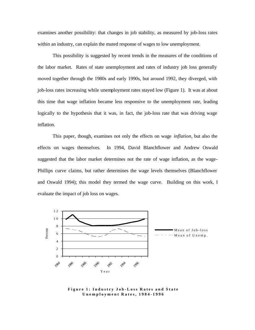
This possibility is suggested by recent trends in the measures of the conditions of

the labor market. Rates of state unemployment and rates of industry job loss generally

moved together through the 1980s and early 1990s, but around 1992, they diverged, with

job-loss rates increasing while unemployment rates stayed low (Figure 1). It was at about

this time that wage inflation became less responsive to the unemployment rate, leading

logically to the hypothesis that it was, in fact, the job-loss rate that was driving wage

inflation.

This paper, though, examines not only the effects on wage inflation, but also the

effects on wages themselves. In 1994, David Blanchflower and Andrew Oswald

suggested that the labor market determines not the rate of wage inflation, as the wage-

Phillips curve claims, but rather determines the wage levels themselves (Blanchflower

and Oswald 1994); this model they termed the wage curve. Building on this work, I

evaluate the impact of job loss on wages.

F i g u r e 1 : I n d u s t r y J o b - L o s s R a t e s a n d S t a t e U n e m p l o y m e n t R a t e s , 1 9 8 4 - 1 9 9 6

0

2

4

6

8

1 0

1 2

1984

1986

1988

1990

1992

1994

1996

Y e a r

Perc

ent M e a n o f J o b - l o s s

M e a n o f U n e m p .

An intuitive mechanism for the connection between job loss and wage levels or

wage inflation may be set forth immediately. It could easily be the case that low

unemployment is found with high rates of job loss: if an industry or firm suffers, it may

displace a large number of workers, but if other areas of the economy are strong enough

to absorb these workers, the overall unemployment rate will remain low (the “Declining-

Industry” hypothesis). The same conditions may be similarly found if the labor market

becomes more volatile for any reason, with people switching jobs frequently (the

“Employee-Turnover” hypothesis). However, if workers have a high cost associated with

losing a job, the possibility of job loss may outweigh the ease of obtaining another job in

the event of job loss in a tight labor market. In other words, workers may not want to or

be able to change jobs for personal reasons even if it’s fairly easy to do so, so in an

environment of high job loss and low unemployment, they will not be as willing to

demand a higher wage as they might when both unemployment and job loss are low.

My empirical findings seem to support this view. Using data from the Displaced

Workers Surveys of 1984 through 1996, I find that, although job loss does not

significantly improve the wage-Phillips curve’s ability to predict or determine rates of

wage inflation, job loss both improves the significance of unemployment and is strongly

significant itself in the wage curve model, its two effects being to lower wage rates and

weaken the sensitivity of wages to the rate of unemployment. Additionally, I find that

the rate of industry job loss is a more consistent predictor of wages than is the rate of

state unemployment, having a “job-loss elasticity of pay” at zero unemployment of –0.3

and an average job-loss elasticity of pay of –0.05 across several demographic variables.

Thus, while augmenting the wage-Phillips curve with job loss appears unnecessary, the

job-loss augmented wage curve appears to be the correct model for assessing the wage-

determining effects of the conditions of the labor market.

I. Job Loss and the Wage-Phillips Curve

Since my initial interest was in the combination of low unemployment and modest

wage inflation, I present my findings on the effects of job-loss rates on the wage-Phillips

curve first. My results show that these effects are not statistically significant: it cannot be

said that job loss alters either wage inflation or the slope of the wage-Phillips curve. The

presentation of these results is preceded by a description of my data and method.

A. Data and Method

To test the hypothesis that the rate of job loss lowers wage inflation and lessens

the sensitivity of wage inflation to the unemployment rate (i.e., lowers the value of the

slope of the wage-Phillips curve), I combine data from three different sources: the web

site of the Bureau of Labor Statistics (BLS), the Annual Earnings File extract of the

Current Population Survey (CPS), and the Displaced Workers Survey (DWS). The BLS

web site provided seasonally adjusted unemployment rates for every state in every month

from January 1978 to October 1998.5 The unemployment rate obtained from the BLS

web site is the standard definition: the number of unemployed at the time of the survey

over the total size of the labor force. To avoid random noise in the data, I use the annual

5 These data may be found at http://stats.bls.gov/sahome.html, selecting “Local Area Unemployment Statistics,” and proceeding with appropriate formatting choices (seasonally adjusted, state-level).

unemployment rate, calculated as the average of the 12 monthly rates for each state.

Job-loss rates are somewhat imprecise, being computed over a three-year period,

because they are calculated from the Displaced Workers Survey. The DWS was a

supplement to the January CPS in every second year from 1984 until 1994, when it was

moved to the February CPS in every second year. The DWS asks a number of questions

pertaining to job loss, but the two most important to this study are the questions asking if

the respondent has lost a job in the previous three years and, if the answer is positive,

from what industry the worker was displaced. Only those who have involuntarily lost a

job are considered displaced workers by the DWS; displacement due to reasons specific

to an individual, such as poor performance or voluntary departure, are not counted. By

virtue of this fact, the rate of job loss that I use is more accurately indicative of the state

of the labor market.

The industry from which the job was lost is recorded according to the Census

Bureau’s three-digit classification system,6 a fact that allows job-loss rates to be

calculated for every industry in every year of the survey. To reduce noise in the data, I

calculate rates of job loss at a two-digit level, using only the first two digits of the three-

digit classification.

In the actual calculation of rates of industry job loss, I adopt the definition used by

Henry Farber in most of his work on rates of aggregate job loss (Farber 1998a, 1998b).

Specifically, job loss is calculated as the number of people who report losing a job in the

previous three years divided by the total number of people currently (that is, at the time

of the survey) in the industry from which the job was lost. I use this method because it is

6 See, for example, http://www.census.gov/apsd/techdoc/cps/mar97/append_a.html.

not computationally difficult and, as Farber notes (1998a, footnote 4), current employees

represent “the pool of workers at risk to be displaced” and the very people whose wages

are likely to be affected by job loss. Further, for the majority of the industry-year cells,

the number of displaced workers is small relative to the current employment pool, in

which case this method provides a good approximation of the risk facing current workers.

Throughout this study, job-loss rates in excess of 100 percent were considered outliers

and excluded from the analysis; in the wage-Phillips curve analysis, there were no such

outliers.

The Annual Earnings File extract from the CPS forms the informational backbone

of my study. The CPS is particularly useful for a study of this sort because of its size and

comprehensiveness. It surveys approximately 60,000 households every month, providing

a concise source of information on earnings, hours worked, and demographics. Further,

with appropriate weighting, it is a representative sample of the U.S. population. For this

study, AEF data for the years 1983 through 1996 were used and limited to males older

than 16 years.

Once the earnings data from the thirteen CPSs are compiled, each observation is

assigned a rate of job loss according to the year and two-digit industry category in which

the worker is employed and a rate of unemployment according to the year and state in

which the worker lives. Specifically, the relevant year is taken to be the year in which

the job-loss and unemployment rates were calculated. Thus, a CPS observation from

1984 is assigned the change in his log wages from 1983 to 1984; the job-loss rate from

the 1984 DWS, which was calculated using displacement over the years 1981 through

1983; and the unemployment rate calculated in 1984. This was done in part to

compensate for an informational lag: job-loss rates are calculated after the fact, but wages

or wage inflation is, if determined by this variable, affected by a similar lag. A worker in

1983 is most likely to have his wages, or the increase in his wages, in 1984 affected by

the job-loss rate that prevails in 1983 but that is calculated in 1984. In the case of odd

years – in which the DWS is not conducted and so rates of job loss not calculated –

observations are assigned a job-loss rate equal to the mean of the job-loss rates of the

years on either side. This is done in an effort to reflect the continuity of the changes in

the labor market.

B. Results and Interpretations

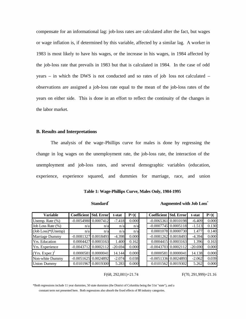
The analysis of the wage-Phillips curve for males is done by regressing the

change in log wages on the unemployment rate, the job-loss rate, the interaction of the

unemployment and job-loss rates, and several demographic variables (education,

experience, experience squared, and dummies for marriage, race, and union

Table 1: Wage-Phillips Curve, Males Only, 1984-1995

Standard* Augmented with Job Loss*

Variable Coefficient Std. Error t-stat P>|t| Coefficient Std. Error t-stat P>|t|Unemp. Rate (%) -0.0054980 0.0007412 -7.418 0.000 -0.0065361 0.0010198 -6.409 0.000Job Loss Rate (%) n/a n/a n/a n/a -0.0007745 0.0005118 -1.513 0.130(Job Loss)*(Unemp) n/a n/a n/a n/a 0.0001078 0.0000730 1.477 0.140Marriage Dummy -0.0081327 0.0018493 -4.398 0.000 -0.0081262 0.0018493 -4.394 0.000Yrs. Education 0.0004427 0.0003163 1.400 0.162 0.0004415 0.0003163 1.396 0.163Yrs. Experience -0.0043712 0.0002112 -20.694 0.000 -0.0043703 0.0002112 -20.690 0.000

(Yrs. Exper.)2 0.0000581 0.0000041 14.144 0.000 0.0000581 0.0000041 14.138 0.000Non-white Dummy -0.0051625 0.0024892 -2.074 0.038 -0.0051336 0.0024893 -2.062 0.039Union Dummy 0.0101967 0.0019300 5.283 0.000 0.0101562 0.0019302 5.262 0.000

F(68, 292,001)=21.74 F(70, 291,999)=21.16

*Both regressions include 11 year dummies, 50 state dummies (the District of Columbia being the 51st "state"), and a

constant term not presented here. Both regressions also absorb the fixed effects of 88 industry categories.

membership). Additionally, dummies for every year but the first (to avoid collinearity)

and every state but one are included to control for the fixed effects of those variables, and

the fixed effects of industry category are absorbed in the regression. The standard wage-

Phillips curve with demographic variables is first estimated, and then terms for job loss

and the interaction of job loss and unemployment are added. The statistics of both

regressions are presented in Table 1.

The results are not definitive, but are also not promising. Adding job loss to the

equation increases the magnitude of the coefficient on unemployment. This result is

consistent with the expectation that job loss lessens the sensitivity of males’ wage

inflation to the unemployment rate: the coefficient on unemployment in the augmented

regression is the effect of unemployment on wage inflation when job loss is zero (a one

percentage point increase in unemployment leads to a 0.6 percent increase in wage

inflation when there is no job loss), whereas the coefficient in the standard model is the

average effect of unemployment on wage inflation for all levels of job loss. Since the

latter is smaller in absolute value, it stands to reason that job loss reduces the sensitivity

of wage inflation to unemployment. Indeed, the direct evidence of this is the positive

coefficient on the interaction term: as the rate of industry job loss increases, the effect of

unemployment on wage inflation becomes less negative; the wage-Phillips curve is

flattened by job-loss. Specifically, according to these results, a one percentage point

increase in the job-loss rate will reduce the magnitude of the effect of unemployment by

about 0.01 percentage points per percentage point of unemployment. Also in accord with

expectations is the slightly negative coefficient on job-loss rate; a one percentage point

increase in the rate of job loss will lower wage inflation directly by almost 0.08 percent.

However, the coefficients on job-loss rate and the interaction term have t-values of about

1.5 in absolute value; this means that there is a probability of 14 percent that job loss has

no effect on wage inflation or the sensitivity of wage inflation to unemployment. While

14 percent is not especially bad, it is not as low as is standard to reject the null hypothesis

– hence my statement that my results in adding job loss to the wage-Phillips curve are

suggestive, but not definitive. I proceed to an analysis of the wage curve, which offers

more promising results.

II. Job Loss and the Wage Curve

Initial results of my analysis of job loss and the wage curve are strongly

supportive of a negative relationship between rates of industry job loss and males’ wages.

These initial results, which are further analyzed in Section III, are presented here, after a

brief description of the data and method used for this analysis.

A. Data Summary

The data used for the wage curve analysis is essentially the same as that used in

the wage-Phillips curve analysis. Data from 1984 through 1996 were used to compile a

data set of over 953,000 observations.

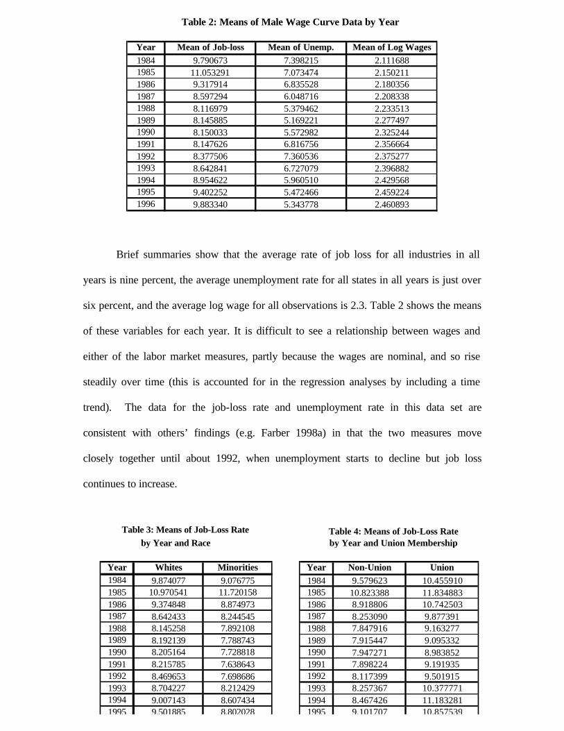
Brief summaries show that the average rate of job loss for all industries in all

years is nine percent, the average unemployment rate for all states in all years is just over

six percent, and the average log wage for all observations is 2.3. Table 2 shows the means

of these variables for each year. It is difficult to see a relationship between wages and

either of the labor market measures, partly because the wages are nominal, and so rise

steadily over time (this is accounted for in the regression analyses by including a time

trend). The data for the job-loss rate and unemployment rate in this data set are

consistent with others’ findings (e.g. Farber 1998a) in that the two measures move

closely together until about 1992, when unemployment starts to decline but job loss

continues to increase.

Table 2: Means of Male Wage Curve Data by Year

Year Mean of Job-loss Mean of Unemp. Mean of Log Wages1984 9.790673 7.398215 2.1116881985 11.053291 7.073474 2.1502111986 9.317914 6.835528 2.1803561987 8.597294 6.048716 2.2083381988 8.116979 5.379462 2.2335131989 8.145885 5.169221 2.2774971990 8.150033 5.572982 2.3252441991 8.147626 6.816756 2.3566641992 8.377506 7.360536 2.3752771993 8.642841 6.727079 2.3968821994 8.954622 5.960510 2.4295681995 9.402252 5.472466 2.4592241996 9.883340 5.343778 2.460893

Table 3: Means of Job-Loss Rate by Year and Race

Year Whites Minorities1984 9.874077 9.0767751985 10.970541 11.7201581986 9.374848 8.8749731987 8.642433 8.2445451988 8.145258 7.8921081989 8.192139 7.7887431990 8.205164 7.7288181991 8.215785 7.6386431992 8.469653 7.6986861993 8.704227 8.2124291994 9.007143 8.6074341995 9.501885 8.802028

Table 4: Means of Job-Loss Rate by Year and Union Membership

Year Non-Union Union1984 9.579623 10.4559101985 10.823388 11.8348831986 8.918806 10.7425031987 8.253090 9.8773911988 7.847916 9.1632771989 7.915447 9.0953321990 7.947271 8.9838521991 7.898224 9.1919351992 8.117399 9.5019151993 8.257367 10.3777711994 8.467426 11.1832811995 9.101707 10.857539

Trends in the rate of industry job loss are also summarized by demographics.

Table 3 shows job-loss rates for minorities and whites. In every year except 1985, whites

have higher job-loss rates than minorities. This does not necessarily mean that whites are

more frequently displaced than minorities, but it does mean that either whites work more

frequently in industries that have high rates of job loss or minorities tend to concentrate

in industries with lower rates of job loss. Union workers have higher rates of job loss for

all years in the data set, as seen in Table 4. This is clearly expected, as it has already

been seen that the industries with the highest rates of job loss are the “heavy” industries,

which are also the industries that have the highest rate of unionization. The high job loss

is almost surely a function of the industry and not of unionization. Both also follow the

trend seen generally over time, although union workers have a slight decline in their rate

of job loss in the last couple of years. This may be associated with the strong demand for

manufactures in the boom economy of the middle 1990s, though even with this slight

decline, the job-loss rate for union workers in the middle 1990s remains significantly

higher than it was in the weak economy of 1990 and 1991.

C. Results and Interpretations

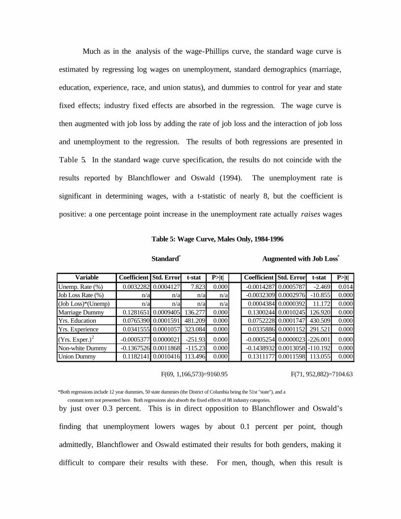
Much as in the analysis of the wage-Phillips curve, the standard wage curve is

estimated by regressing log wages on unemployment, standard demographics (marriage,

education, experience, race, and union status), and dummies to control for year and state

fixed effects; industry fixed effects are absorbed in the regression. The wage curve is

then augmented with job loss by adding the rate of job loss and the interaction of job loss

and unemployment to the regression. The results of both regressions are presented in

Table 5. In the standard wage curve specification, the results do not coincide with the

results reported by Blanchflower and Oswald (1994). The unemployment rate is

significant in determining wages, with a t-statistic of nearly 8, but the coefficient is

positive: a one percentage point increase in the unemployment rate actually raises wages

by just over 0.3 percent. This is in direct opposition to Blanchflower and Oswald’s

finding that unemployment lowers wages by about 0.1 percent per point, though

admittedly, Blanchflower and Oswald estimated their results for both genders, making it

difficult to compare their results with these. For men, though, when this result is

Table 5: Wage Curve, Males Only, 1984-1996


Variable Coefficient Std. Error t-stat P>|t| Coefficient Std. Error t-stat P>|t|Unemp. Rate (%) 0.0032282 0.0004127 7.823 0.000 -0.0014287 0.0005787 -2.469 0.014Job Loss Rate (%) n/a n/a n/a n/a -0.0032309 0.0002976 -10.855 0.000(Job Loss)*(Unemp) n/a n/a n/a n/a 0.0004384 0.0000392 11.172 0.000Marriage Dummy 0.1281651 0.0009405 136.277 0.000 0.1300244 0.0010245 126.920 0.000Yrs. Education 0.0765390 0.0001591 481.209 0.000 0.0752228 0.0001747 430.509 0.000Yrs. Experience 0.0341555 0.0001057 323.084 0.000 0.0335886 0.0001152 291.521 0.000

(Yrs. Exper.)2 -0.0005377 0.0000021 -251.93 0.000 -0.0005254 0.0000023 -226.001 0.000Non-white Dummy -0.1367526 0.0011868 -115.23 0.000 -0.1438932 0.0013058 -110.192 0.000Union Dummy 0.1182141 0.0010416 113.496 0.000 0.1311177 0.0011598 113.055 0.000

F(69, 1,166,573)=9160.95 F(71, 952,882)=7104.63



combined with the strong results of unemployment’s effects on wage inflation, the

findings suggest support of the traditional Phillips curve over the standard wage curve.

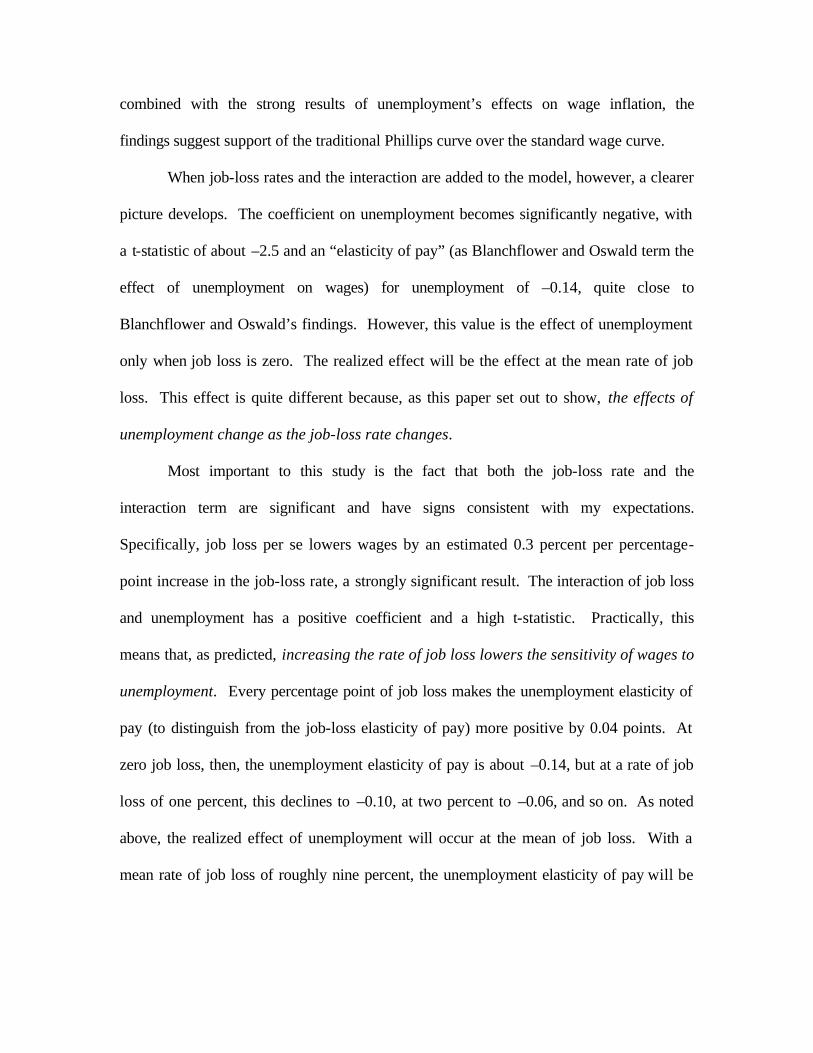
When job-loss rates and the interaction are added to the model, however, a clearer

picture develops. The coefficient on unemployment becomes significantly negative, with

a t-statistic of about –2.5 and an “elasticity of pay” (as Blanchflower and Oswald term the

effect of unemployment on wages) for unemployment of –0.14, quite close to

Blanchflower and Oswald’s findings. However, this value is the effect of unemployment

only when job loss is zero. The realized effect will be the effect at the mean rate of job

loss. This effect is quite different because, as this paper set out to show, the effects of

unemployment change as the job-loss rate changes.

Most important to this study is the fact that both the job-loss rate and the

interaction term are significant and have signs consistent with my expectations.

Specifically, job loss per se lowers wages by an estimated 0.3 percent per percentage-

point increase in the job-loss rate, a strongly significant result. The interaction of job loss

and unemployment has a positive coefficient and a high t-statistic. Practically, this

means that, as predicted, increasing the rate of job loss lowers the sensitivity of wages to

unemployment. Every percentage point of job loss makes the unemployment elasticity of

pay (to distinguish from the job-loss elasticity of pay) more positive by 0.04 points. At

zero job loss, then, the unemployment elasticity of pay is about –0.14, but at a rate of job

loss of one percent, this declines to –0.10, at two percent to –0.06, and so on. As noted

above, the realized effect of unemployment will occur at the mean of job loss. With a

mean rate of job loss of roughly nine percent, the unemployment elasticity of pay will be

positive – about 0.22, not dissimilar from the result obtained by estimating the wage

curve without controlling for job loss.

These results imply, in fact, that for any industry job-loss rate over roughly 3.5

percent, the unemployment elasticity of pay will be positive in that industry. Whereas the

result found by Blanchflower and Oswald predicts that wages will be higher in periods of

low unemployment, the result found here predicts that wages will be higher in periods of

low unemployment only if the job-loss rate is also low. With high rates of job loss, not

only are wages lowered by the job loss directly, but the effect of low unemployment

(which would tend to raise wags) is lessened. Indeed, with sufficiently high rates of job

loss, the unemployment-wage relationship becomes positive, so that a decline in

unemployment will serve to lower wages further, reinforcing the wage-decreasing effect

of high job loss.

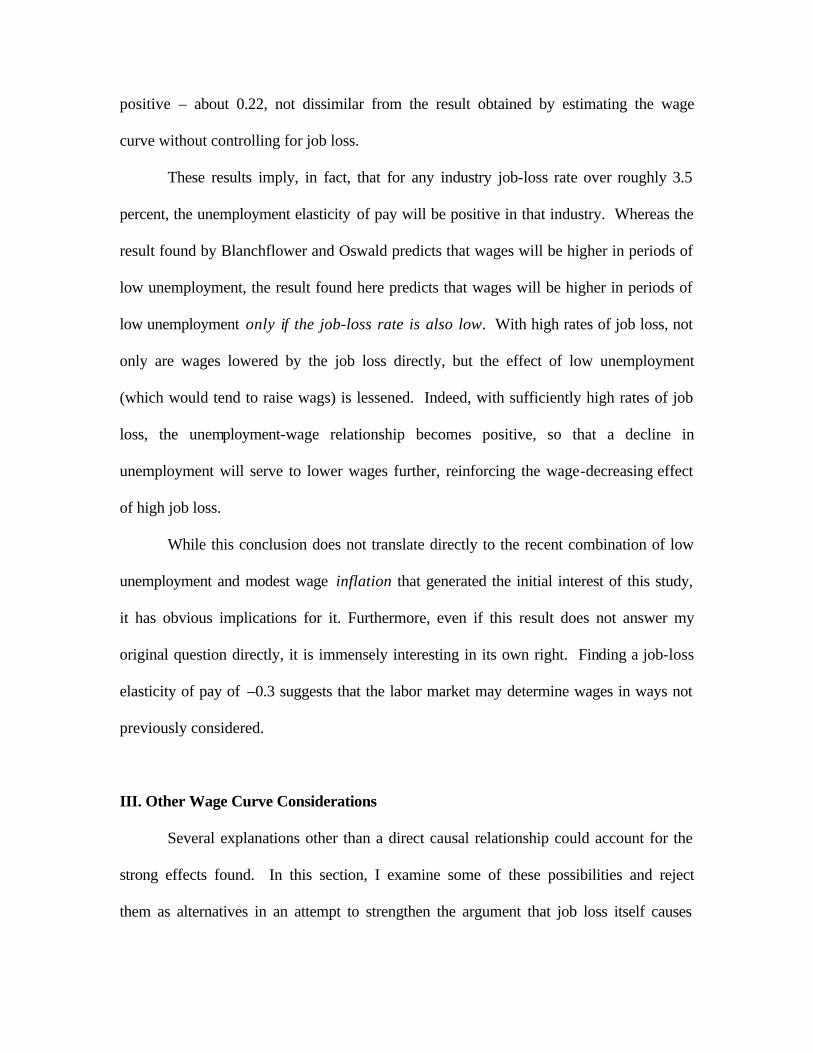
While this conclusion does not translate directly to the recent combination of low

unemployment and modest wage inflation that generated the initial interest of this study,

it has obvious implications for it. Furthermore, even if this result does not answer my

original question directly, it is immensely interesting in its own right. Finding a job-loss

elasticity of pay of –0.3 suggests that the labor market may determine wages in ways not

previously considered.

III. Other Wage Curve Considerations

Several explanations other than a direct causal relationship could account for the

strong effects found. In this section, I examine some of these possibilities and reject

them as alternatives in an attempt to strengthen the argument that job loss itself causes

wages to be lower and less sensitive to unemployment. This is done with respect to the

following: first, compositional biases, the notion that the demographic composition of the

labor force in an industry will affect its wages; second, declining industries, as opposed to

employee turnover (see p. 3); third, inaccurate standard errors; and fourth, variations in

the specification of the job-loss augmented wage curve.

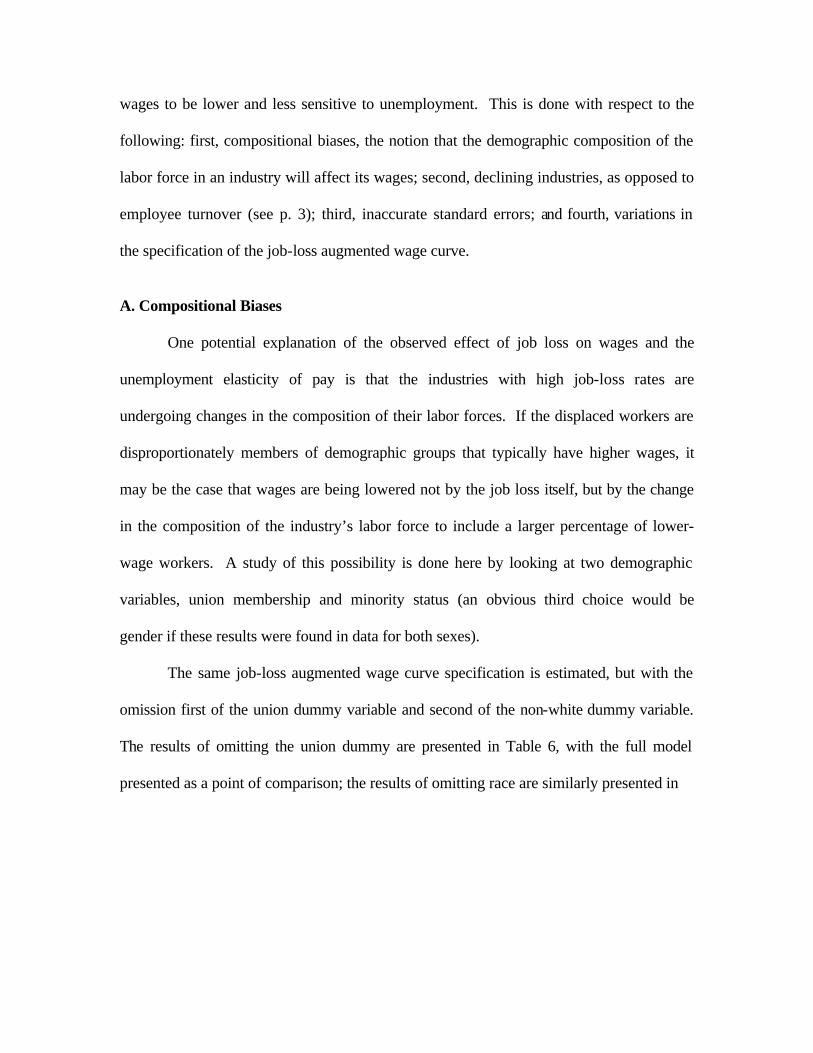
A. Compositional Biases

One potential explanation of the observed effect of job loss on wages and the

unemployment elasticity of pay is that the industries with high job-loss rates are

undergoing changes in the composition of their labor forces. If the displaced workers are

disproportionately members of demographic groups that typically have higher wages, it

may be the case that wages are being lowered not by the job loss itself, but by the change

in the composition of the industry’s labor force to include a larger percentage of lower-

wage workers. A study of this possibility is done here by looking at two demographic

variables, union membership and minority status (an obvious third choice would be

gender if these results were found in data for both sexes).

The same job-loss augmented wage curve specification is estimated, but with the

omission first of the union dummy variable and second of the non-white dummy variable.

The results of omitting the union dummy are presented in Table 6, with the full model

presented as a point of comparison; the results of omitting race are similarly presented in

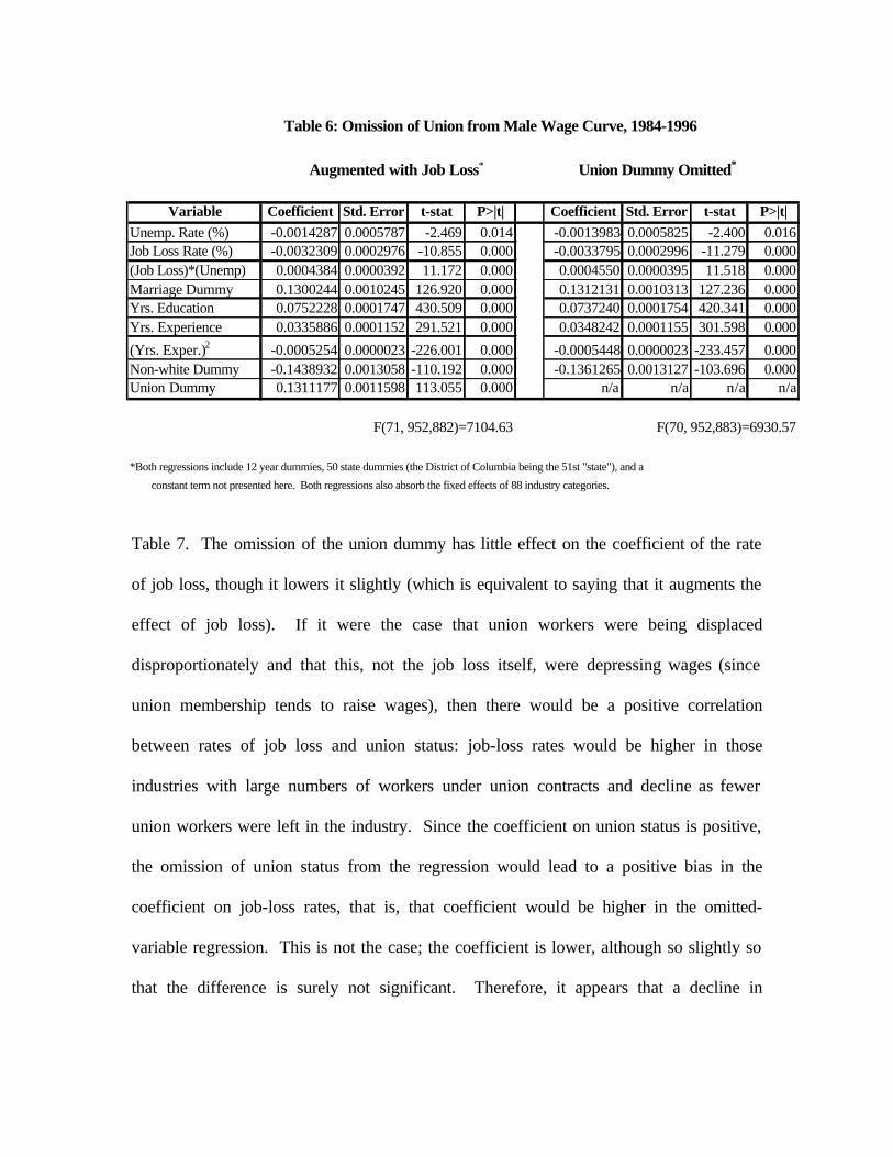
Table 7. The omission of the union dummy has little effect on the coefficient of the rate

of job loss, though it lowers it slightly (which is equivalent to saying that it augments the

effect of job loss). If it were the case that union workers were being displaced

disproportionately and that this, not the job loss itself, were depressing wages (since

union membership tends to raise wages), then there would be a positive correlation

between rates of job loss and union status: job-loss rates would be higher in those

industries with large numbers of workers under union contracts and decline as fewer

union workers were left in the industry. Since the coefficient on union status is positive,

the omission of union status from the regression would lead to a positive bias in the

coefficient on job-loss rates, that is, that coefficient would be higher in the omitted-

variable regression. This is not the case; the coefficient is lower, although so slightly so

that the difference is surely not significant. Therefore, it appears that a decline in

Table 6: Omission of Union from Male Wage Curve, 1984-1996

Augmented with Job Loss* Union Dummy Omitted*

Variable Coefficient Std. Error t-stat P>|t| Coefficient Std. Error t-stat P>|t|Unemp. Rate (%) -0.0014287 0.0005787 -2.469 0.014 -0.0013983 0.0005825 -2.400 0.016Job Loss Rate (%) -0.0032309 0.0002976 -10.855 0.000 -0.0033795 0.0002996 -11.279 0.000(Job Loss)*(Unemp) 0.0004384 0.0000392 11.172 0.000 0.0004550 0.0000395 11.518 0.000Marriage Dummy 0.1300244 0.0010245 126.920 0.000 0.1312131 0.0010313 127.236 0.000Yrs. Education 0.0752228 0.0001747 430.509 0.000 0.0737240 0.0001754 420.341 0.000Yrs. Experience 0.0335886 0.0001152 291.521 0.000 0.0348242 0.0001155 301.598 0.000

(Yrs. Exper.)2 -0.0005254 0.0000023 -226.001 0.000 -0.0005448 0.0000023 -233.457 0.000Non-white Dummy -0.1438932 0.0013058 -110.192 0.000 -0.1361265 0.0013127 -103.696 0.000Union Dummy 0.1311177 0.0011598 113.055 0.000 n/a n/a n/a n/a

F(71, 952,882)=7104.63 F(70, 952,883)=6930.57



unionization is not responsible for the observed effect of job-loss rates on wages and the

unemployment elasticity of pay.

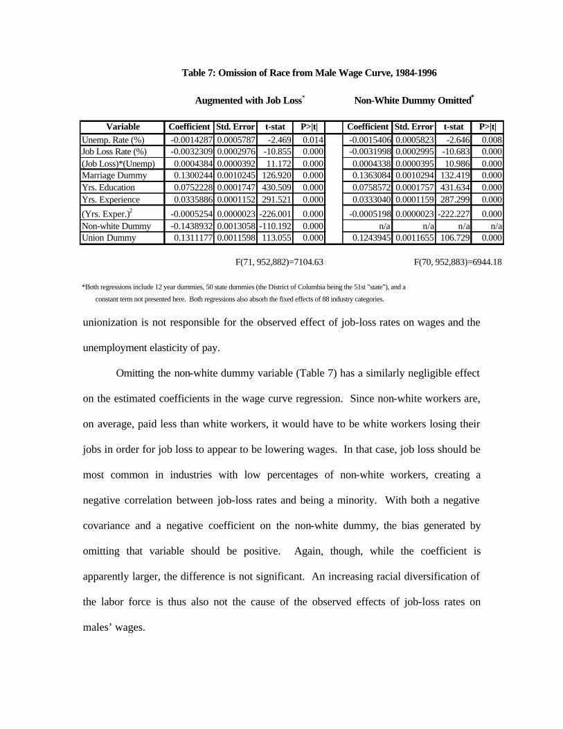
Omitting the non-white dummy variable (Table 7) has a similarly negligible effect

on the estimated coefficients in the wage curve regression. Since non-white workers are,

on average, paid less than white workers, it would have to be white workers losing their

jobs in order for job loss to appear to be lowering wages. In that case, job loss should be

most common in industries with low percentages of non-white workers, creating a

negative correlation between job-loss rates and being a minority. With both a negative

covariance and a negative coefficient on the non-white dummy, the bias generated by

omitting that variable should be positive. Again, though, while the coefficient is

apparently larger, the difference is not significant. An increasing racial diversification of

the labor force is thus also not the cause of the observed effects of job-loss rates on

males’ wages.

Table 7: Omission of Race from Male Wage Curve, 1984-1996

Augmented with Job Loss* Non-White Dummy Omitted*


(Yrs. Exper.)2 -0.0005254 0.0000023 -226.001 0.000 -0.0005198 0.0000023 -222.227 0.000Non-white Dummy -0.1438932 0.0013058 -110.192 0.000 n/a n/a n/a n/aUnion Dummy 0.1311177 0.0011598 113.055 0.000 0.1243945 0.0011655 106.729 0.000

F(71, 952,882)=7104.63 F(70, 952,883)=6944.18



While many other potential compositional biases that could be driving this result

surely exist, these two – unionization and race – are two of the most likely, given their

plausibility under recent trends in the labor force and their significant effects on wages

(again, the third likely factor, gender, was deliberately eliminated at the beginning of the

study). With these two possibilities eliminated, it is much safer to say that the negative

effect of job loss is not due to a systematic shift in the composition of the labor force.

B. Declining Industries v. Employee Turnover

As suggested earlier, high rates of job loss may indicate one of two conditions:

either the labor demand in an industry as a whole is declining, so that workers are being

displaced without being replaced; or the industry is characterized by high employee

turnover, so that workers are replaced with new workers as they are displaced. If the

former case dominates, then my results are somewhat less interesting, since displaced

workers would have to find employment in different industries and most likely in

industries in which they have less expertise – which would naturally depress wages. Job

loss would not be directly responsible for the wage decline.

This could be an argument for the use of a measure of industry-specific training or

experience, rather than the general experience measure used here, but such an industry-

specific measure is not available from the CPS. Instead, I estimate trends in turnover by

looking at employment levels in each industry based on males’ CPS responses from 1984

through 1996. If employment levels decline significantly, this is evidence that the

industry is declining, or at least in the trough of a cyclical employment pattern, which

would have the same effects. Hence, to say as I want that the job-loss rate is directly

responsible for the effect on wages, such a decline must be ruled out as a general pattern.

Employment in an industry was calculated both as an absolute figure – the number of

people who reported being employed and working in that industry – and as a percentage

of all employed people in the labor force, providing a measure of relative decline.

If I were to find a strong correlation between the rate of job loss and either of the

measures of industry employment, then I would have to say that job loss could be

indicating a declining industry rather than employee turnover. This is not the case,

though. The rate of job loss is, in fact, only weakly correlated with either measure, if at

all. The coefficient of correlation between the rate of job loss and the number of

employees in an industry is found to be 0.1139, and the coefficient between the rate of

job loss and the employment percentage in an industry is found to be only 0.1217. With

these figures, it is safe to conclude that job loss does not move closely with industry

employment. It is not capturing the effects of an industry’s decline.

It is also possible to judge the effects of declining industries on the job-loss

augmented wage curve by excluding those industries from the regression analysis. The

employment percentage is used as the evaluative statistic for this purpose because only

relative declines would affect the impact of job loss on wages; if all industries are

declining, as could be captured by levels of employment, either unemployment is

increasing, which has an effect on wages that is not the point of this study, or the labor

force is shrinking, which should lead to higher wages, not the lower wages that are

correlated with a higher rate of job loss. It can be found that the largest declines over the

period in question came in Machinery and Computing Equipment and Mining. Results of

the regression that excludes these declining industries are shown in Table 8, again with

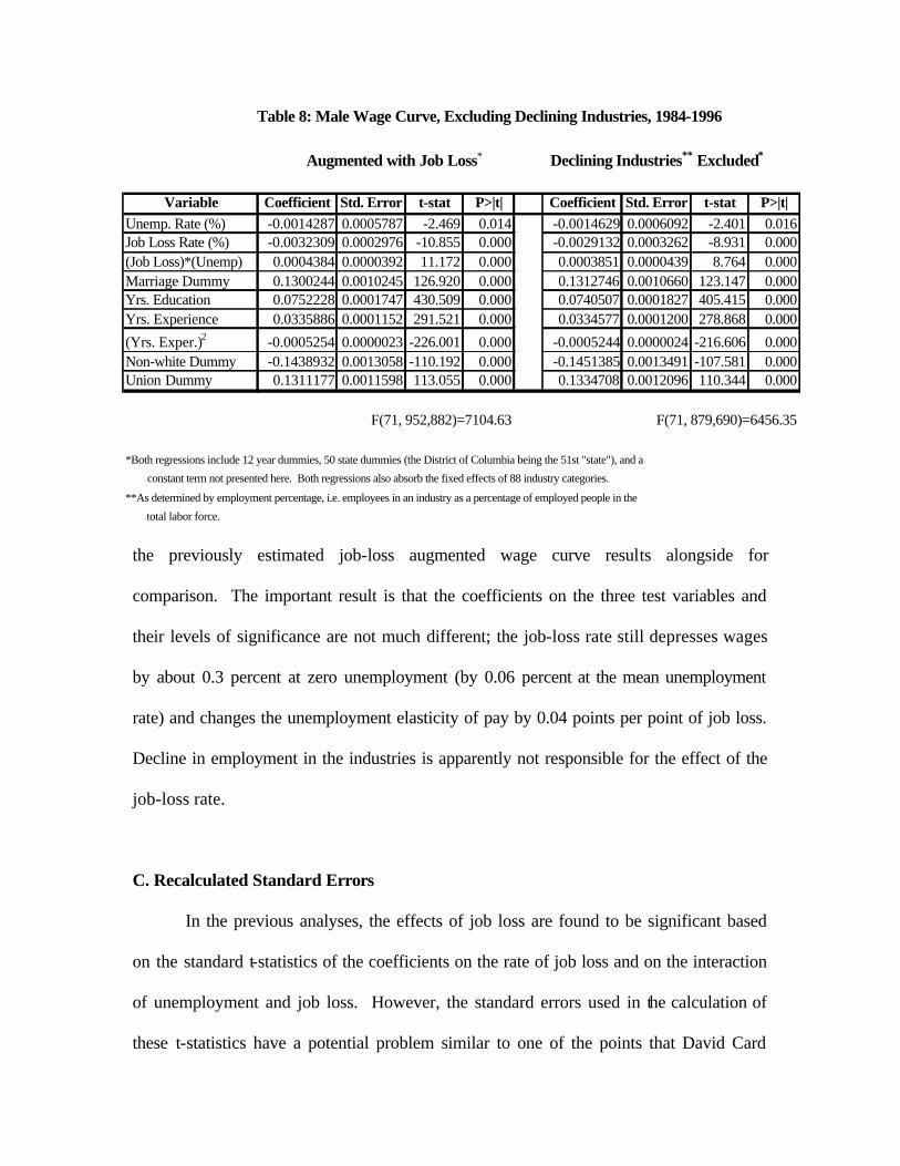
the previously estimated job-loss augmented wage curve results alongside for

comparison. The important result is that the coefficients on the three test variables and

their levels of significance are not much different; the job-loss rate still depresses wages

by about 0.3 percent at zero unemployment (by 0.06 percent at the mean unemployment

rate) and changes the unemployment elasticity of pay by 0.04 points per point of job loss.

Decline in employment in the industries is apparently not responsible for the effect of the

job-loss rate.

C. Recalculated Standard Errors

In the previous analyses, the effects of job loss are found to be significant based

on the standard t-statistics of the coefficients on the rate of job loss and on the interaction

of unemployment and job loss. However, the standard errors used in the calculation of

these t-statistics have a potential problem similar to one of the points that David Card

Table 8: Male Wage Curve, Excluding Declining Industries, 1984-1996

Augmented with Job Loss* Declining Industries** Excluded*



F(71, 952,882)=7104.63 F(71, 879,690)=6456.35



**As determined by employment percentage, i.e. employees in an industry as a percentage of employed people in the

total labor force.

notes in his (1995) review of Blanchflower and Oswald’s book, The Wage Curve. These

standard errors are based on the number of individual observations, but as Card writes,

“the actual ‘degrees of freedom’ involved in the estimation of the wage curve elasticity is

far less than the number of individual wage observations. Indeed, the relevant dimension

for the estimation of the unemployment coefficient is the number of regional labor

markets times the number of time periods” (p. 7). In other words, standard errors must be

calculated at the smallest level of variation in the relevant variable. In this study, all

individuals in the same year and industry have the same rate of job loss, all in the same

year and state have the same rate of unemployment, and all in the same year-state-

industry cell have the same value for the interaction term. Calculating standard errors at

the individual level will therefore lead to a large downward bias in those errors, which

leads to t-statistics that will overstate the significance of those variables.

One solution to this problem – and the one adopted here – is to collapse the data

onto the mean of the variables within the state-industry-year cell. This aggregation

method is quite similar to Blanchflower and Oswald’s approach to this problem, and is

good in that it accounts for most of the bias in the standard errors and is fairly simple to

do. It is not ideal, though, since this method can lead to imprecise estimates of the

coefficients on the control variables. It will also alter the coefficients of the test variables

if the cells are not weighted by the number of observations in each; cells with many

observations will have the same impact on the results as cells with few observations if

they are merely collapsed onto their means without weighting. This weighting is not

difficult, and is used here, so all coefficients presented in the tables are valid for analysis.

Some discrepancy between the aggregated-data and individual-data coefficients remains,

but this method works well for judging the bias in the standard errors of the variables this

study is most interested in.

Using this aggregation method on the standard wage curve and the job-loss

augmented wage curve leads to the results presented in Table 9 (next page). For

comparison, I have reproduced beside it Table 5, which shows the same results for the

original, uncollapsed data. In the case of the standard wage curve, observations are

aggregated over the larger state-year cells, rather than state-year-industry cells, since no

variation occurs across industry categories. This leads to insignificance in some of the

demographic variables, but this may be due to the imprecision in the control variables

that Card noted. This also accounts for the fact that the standard errors of the augmented

model are smaller than in the standard wage curve model. Note, though, that the standard

errors for the collapsed data are larger in all cases than the corresponding figures for the

uncollapsed data (comparing the standard errors in Table 9, which uses collapsed data,

with those in Table 5).

The result that is consequential to this study is the fact that both the job-loss rate

and the interaction are still significant at less than one percent, even with the larger

standard errors. They also still have the expected sign, and the effects, as they should be,

are roughly the same. An additional percentage point in the job-loss rate still lowers

wages by about 0.3 percent at zero unemployment (again, the effect at the mean

unemployment rate is about 0.06 percent) and lowers the magnitude of the

unemployment elasticity of pay by about .04 percentage points. The same result holds

for the unemployment rate in the job-loss augmented model, as it is significant and

consistent with the idea of the wage curve at zero job loss, though the unemployment

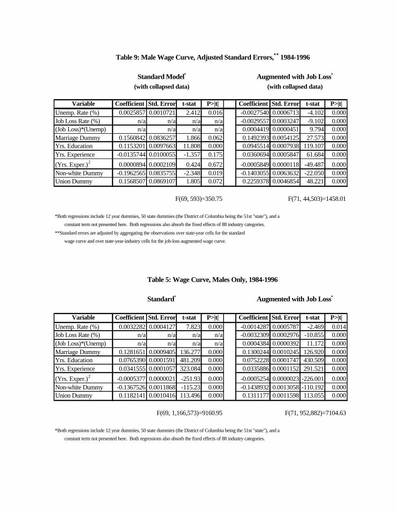
Table 9: Male Wage Curve, Adjusted Standard Errors,** 1984-1996

Standard Model* Augmented with Job Loss*

(with collapsed data) (with collapsed data)

Variable Coefficient Std. Error t-stat P>|t| Coefficient Std. Error t-stat P>|t|Unemp. Rate (%) 0.0025857 0.0010721 2.412 0.016 -0.0027540 0.0006713 -4.102 0.000Job Loss Rate (%) n/a n/a n/a n/a -0.0029557 0.0003247 -9.102 0.000(Job Loss)*(Unemp) n/a n/a n/a n/a 0.0004419 0.0000451 9.794 0.000Marriage Dummy 0.1560842 0.0836257 1.866 0.062 0.1492393 0.0054125 27.573 0.000Yrs. Education 0.1153201 0.0097663 11.808 0.000 0.0945514 0.0007938 119.107 0.000Yrs. Experience -0.0135744 0.0100055 -1.357 0.175 0.0360694 0.0005847 61.684 0.000

(Yrs. Exper.)2 0.0000894 0.0002109 0.424 0.672 -0.0005849 0.0000118 -49.487 0.000Non-white Dummy -0.1962565 0.0835755 -2.348 0.019 -0.1403055 0.0063632 -22.050 0.000Union Dummy 0.1568507 0.0869107 1.805 0.072 0.2259378 0.0046854 48.221 0.000

F(69, 593)=350.75 F(71, 44,503)=1458.01



**Standard errors are adjusted by aggregating the observations over state-year cells for the standard

wage curve and over state-year-industry cells for the job-loss augmented wage curve.

Table 5: Wage Curve, Males Only, 1984-1996


Variable Coefficient Std. Error t-stat P>|t| Coefficient Std. Error t-stat P>|t|Unemp. Rate (%) 0.0032282 0.0004127 7.823 0.000 -0.0014287 0.0005787 -2.469 0.014Job Loss Rate (%) n/a n/a n/a n/a -0.0032309 0.0002976 -10.855 0.000(Job Loss)*(Unemp) n/a n/a n/a n/a 0.0004384 0.0000392 11.172 0.000Marriage Dummy 0.1281651 0.0009405 136.277 0.000 0.1300244 0.0010245 126.920 0.000Yrs. Education 0.0765390 0.0001591 481.209 0.000 0.0752228 0.0001747 430.509 0.000Yrs. Experience 0.0341555 0.0001057 323.084 0.000 0.0335886 0.0001152 291.521 0.000


F(69, 1,166,573)=9160.95 F(71, 952,882)=7104.63



elasticity of pay here is somewhat larger than that estimated by Blanchflower and Oswald

(1994). With a positive and significant coefficient on the interaction term, this observed

negative effect of the unemployment rate will get smaller as the rate of industry job loss

increases, so that at the mean rate of job loss, the effect of unemployment is zero or

positive, which is not consistent with the wage curve.

The significance of the test variables in this analysis is a crucial result. Even with

the upwardly adjusted standard errors, the effects of the rate of job loss on both wages

and the unemployment elasticity of pay are strongly significant, a fact that makes my

conclusion – that the rate of industry job loss is as important a measure of the state of the

labor market as the state unemployment rate is – much stronger.

D. Variations in the Effects of the Job-Loss Rate

The effects of the rate of job loss on males’ wages may be altered by a number of

variables. This section presents some descriptive data (descriptive in that the differences

are not rigorously tested in most cases) of the differences in those effects across several

demographic variables. It must be noted beforehand that, in investigating the differences

across demographic groups, other demographic variables are excluded. This omission

has at most a negligible bearing on this discussion.

D.1. MINORITY V. WHITE

When the data are divided on the basis of minority status, we see that the effects

of the job-loss rate are roughly the same for whites and minorities, but the wages of

minorities are much more responsive to the unemployment rate than are those of white

workers (Table 10). Also, the job-loss elasticity of pay at zero unemployment is again

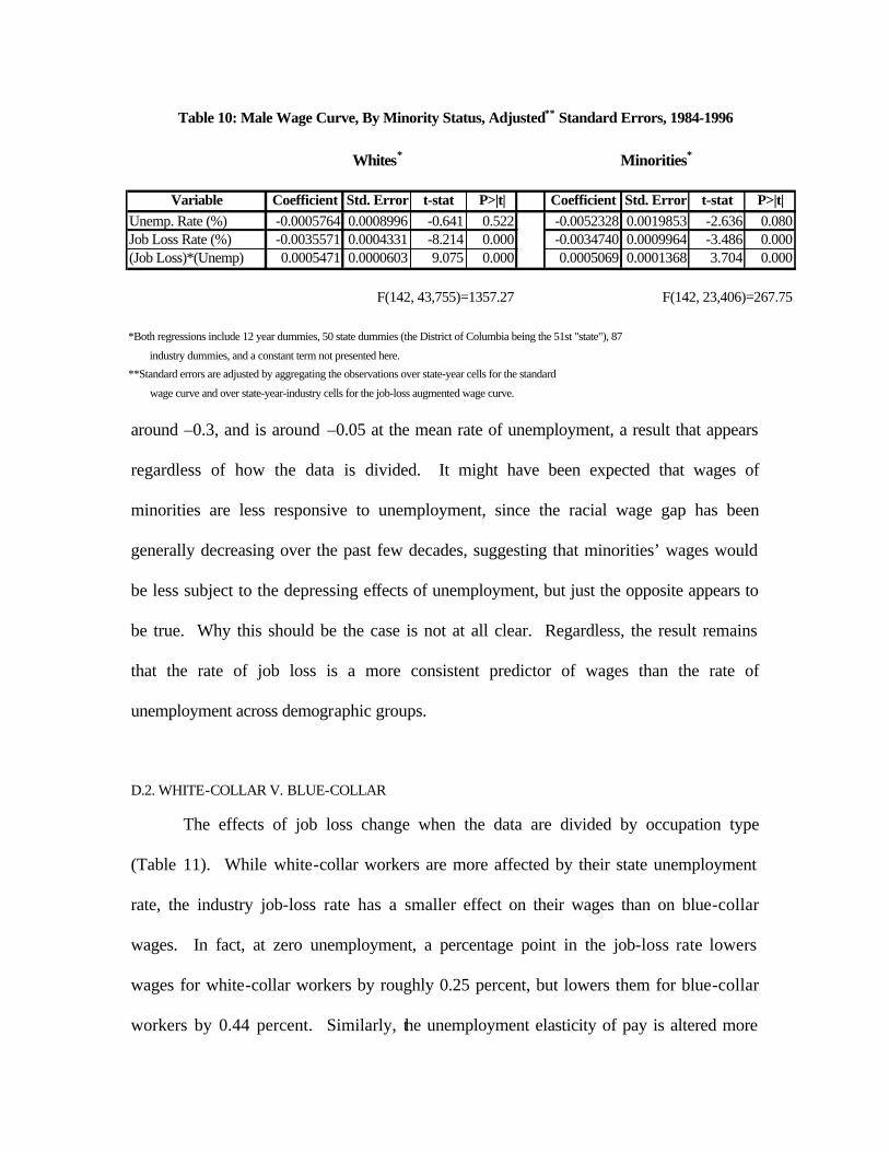
around –0.3, and is around –0.05 at the mean rate of unemployment, a result that appears

regardless of how the data is divided. It might have been expected that wages of

minorities are less responsive to unemployment, since the racial wage gap has been

generally decreasing over the past few decades, suggesting that minorities’ wages would

be less subject to the depressing effects of unemployment, but just the opposite appears to

be true. Why this should be the case is not at all clear. Regardless, the result remains

that the rate of job loss is a more consistent predictor of wages than the rate of

unemployment across demographic groups.

D.2. WHITE-COLLAR V. BLUE-COLLAR

The effects of job loss change when the data are divided by occupation type

(Table 11). While white-collar workers are more affected by their state unemployment

rate, the industry job-loss rate has a smaller effect on their wages than on blue-collar

wages. In fact, at zero unemployment, a percentage point in the job-loss rate lowers

wages for white-collar workers by roughly 0.25 percent, but lowers them for blue-collar

workers by 0.44 percent. Similarly, the unemployment elasticity of pay is altered more

Table 10: Male Wage Curve, By Minority Status, Adjusted** Standard Errors, 1984-1996

Whites* Minorities*

Variable Coefficient Std. Error t-stat P>|t| Coefficient Std. Error t-stat P>|t|Unemp. Rate (%) -0.0005764 0.0008996 -0.641 0.522 -0.0052328 0.0019853 -2.636 0.080Job Loss Rate (%) -0.0035571 0.0004331 -8.214 0.000 -0.0034740 0.0009964 -3.486 0.000(Job Loss)*(Unemp) 0.0005471 0.0000603 9.075 0.000 0.0005069 0.0001368 3.704 0.000

F(142, 43,755)=1357.27 F(142, 23,406)=267.75

*Both regressions include 12 year dummies, 50 state dummies (the District of Columbia being the 51st "state"), 87

industry dummies, and a constant term not presented here.



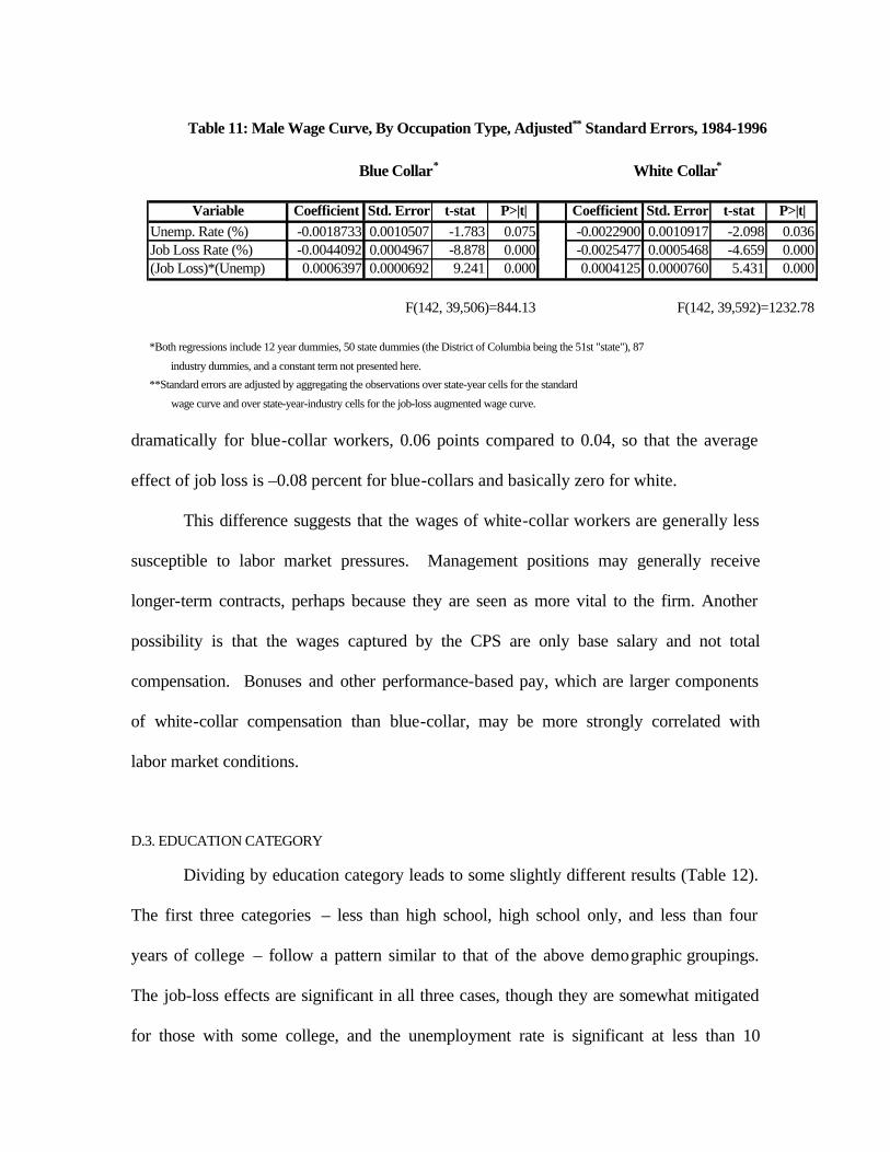
dramatically for blue-collar workers, 0.06 points compared to 0.04, so that the average

effect of job loss is –0.08 percent for blue-collars and basically zero for white.

This difference suggests that the wages of white-collar workers are generally less

susceptible to labor market pressures. Management positions may generally receive

longer-term contracts, perhaps because they are seen as more vital to the firm. Another

possibility is that the wages captured by the CPS are only base salary and not total

compensation. Bonuses and other performance-based pay, which are larger components

of white-collar compensation than blue-collar, may be more strongly correlated with

labor market conditions.

D.3. EDUCATION CATEGORY

Dividing by education category leads to some slightly different results (Table 12).

The first three categories – less than high school, high school only, and less than four

years of college – follow a pattern similar to that of the above demographic groupings.

The job-loss effects are significant in all three cases, though they are somewhat mitigated

for those with some college, and the unemployment rate is significant at less than 10

Table 11: Male Wage Curve, By Occupation Type, Adjusted** Standard Errors, 1984-1996

Blue Collar* White Collar*


F(142, 39,506)=844.13 F(142, 39,592)=1232.78

*Both regressions include 12 year dummies, 50 state dummies (the District of Columbia being the 51st "state"), 87




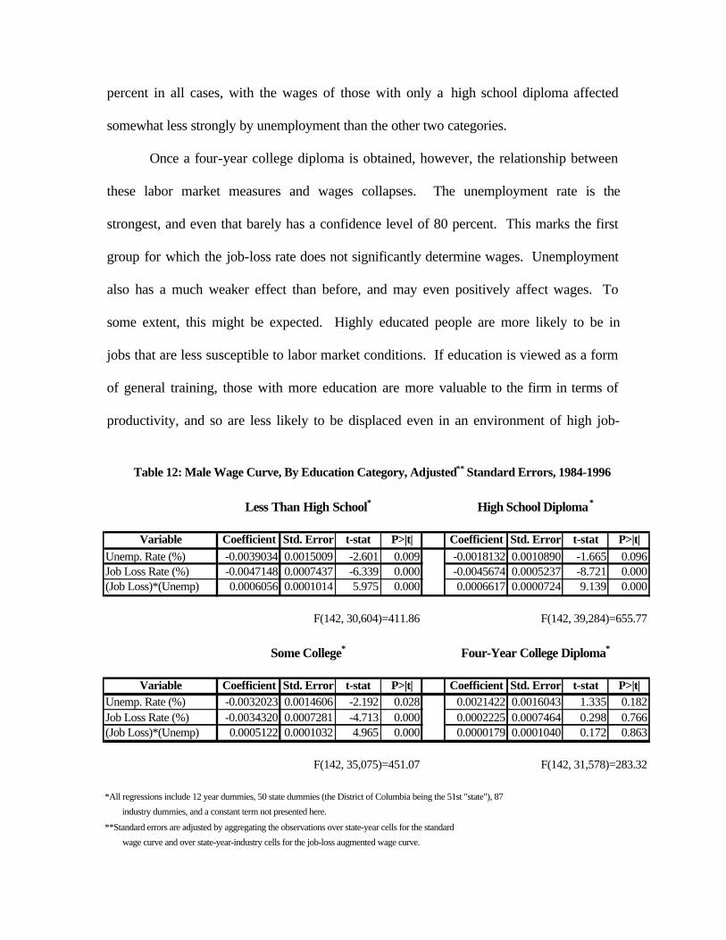
percent in all cases, with the wages of those with only a high school diploma affected

somewhat less strongly by unemployment than the other two categories.

Once a four-year college diploma is obtained, however, the relationship between

these labor market measures and wages collapses. The unemployment rate is the

strongest, and even that barely has a confidence level of 80 percent. This marks the first

group for which the job-loss rate does not significantly determine wages. Unemployment

also has a much weaker effect than before, and may even positively affect wages. To

some extent, this might be expected. Highly educated people are more likely to be in

jobs that are less susceptible to labor market conditions. If education is viewed as a form

of general training, those with more education are more valuable to the firm in terms of

productivity, and so are less likely to be displaced even in an environment of high job-

Table 12: Male Wage Curve, By Education Category, Adjusted** Standard Errors, 1984-1996

Less Than High School* High School Diploma*


F(142, 30,604)=411.86 F(142, 39,284)=655.77

Some College* Four-Year College Diploma*

Variable Coefficient Std. Error t-stat P>|t| Coefficient Std. Error t-stat P>|t|Unemp. Rate (%) -0.0032023 0.0014606 -2.192 0.028 0.0021422 0.0016043 1.335 0.182Job Loss Rate (%) -0.0034320 0.0007281 -4.713 0.000 0.0002225 0.0007464 0.298 0.766(Job Loss)*(Unemp) 0.0005122 0.0001032 4.965 0.000 0.0000179 0.0001040 0.172 0.863

F(142, 35,075)=451.07 F(142, 31,578)=283.32

*All regressions include 12 year dummies, 50 state dummies (the District of Columbia being the 51st "state"), 87




loss rates. With less risk, their wages will not suffer the same negative effects of a slack

labor market. Indeed, because they are more valuable to the firm, employers will be

more willing to give longer-term contracts specifically because the value to the firm of

highly trained workers will not change with the cycles of the economy, whereas a worker

who is only marginally beneficial in a strong economy is at great risk if the firm finds it

necessary to cut costs in a weak economy. With longer-term contracts, then, the wages of

highly educated people will be less procyclical, which is precisely the result obtained

here.

IV. Conclusion

This study has attempted to redefine the wage-Phillips curve and the wage curve,

as first proposed by Blanchflower and Oswald (1994), by augmenting both models with

a second measure of the prevailing conditions in the labor market: the rate of job loss

within an industry. Success for the wage-Phillips curve is little if any, but the wage curve

results are much stronger. Surely, my results can only be regarded as preliminary, but

they are definitive within the scope of this study, and seem to support expanding the

scope. The major results found here may be summarized as follows:

1. The job-loss augmented model of the wage-Phillips curve cannot be supported, as the

rate of industry job loss does not appear to determine or predict wage inflation. Job-

loss rates are only weakly, if at all, significant in a wage-Phillips curve for males.

2. The job-loss augmented model of the wage curve is strongly supported. The rates of

industry job loss have a significant and negative effect on males’ wages and a

significant and positive effect on the unemployment elasticity of pay (as defined by

Blanchflower and Oswald (1994)). As the unemployment elasticity of pay is

negative, this means that industry job loss weakens the negative sensitivity of males’

wages to state unemployment.

3. The estimated job-loss elasticity of pay at zero unemployment is consistently around

–0.3. The average effect of job loss, that is, the job-loss elasticity of pay at the mean

rate of unemployment, is consistently around –0.05. This is true across several

demographic variables, including union status, race, and marital status.7

4. Across these demographic variables, the rate of industry job loss is a much more

consistent predictor of wages than is the rate of state unemployment, as the job-loss

elasticity of pay remains about the same in all cases, while the unemployment

elasticity of pay varies greatly.

5. The job-loss elasticity of pay does vary across education levels, experience levels,

occupation types, and industry categories.7 Specifically, those with more education

or more experience are insulated from the effects of both industry job loss and state

unemployment on their wages, consistent with the hypothesis that the accumulation

of human capital lessens the susceptibility of one’s wages to labor market conditions.

White-collar workers are also less affected in their wages by the tightness of the labor

market, though the effects on other types of compensation, such as bonuses, are not

studied here.

6. The effects of job loss, both on wages and on the unemployment elasticity of pay,

remain significant at less than 0.1 percent (a confidence level of 99.9 percent

associated with t-statistics of over nine in both cases) and the coefficients change

7 To conserve space, the analysis of some of these demographic variables has not been included. For full results, contact the author.

little when standard errors are adjusted by collapsing the data on to means within

state-year-industry cells.

7. The observed effects of rates of industry job loss do not appear to be caused by

changes in the racial composition (looking at whites versus non-whites) of the labor

force within an industry or by changes in an industry’s rate of unionization.

8. The observed effects of rates of industry job loss also do not appear to be caused by a

decline in the size of an industry’s labor force, suggesting that the measured rate of

job loss is instead correlated with employee turnover.

Future studies may endeavor to examine the differences between actual rates of

industry job loss, which I have used here, and perceptions of job security. While actual

job loss produces strong results in a wage curve model, it may be that perceptions of job

security come closer to explaining the observation I originally sought to understand, the

combination of low rates of unemployment and modest wage inflation. Some work in

this area has already been done by Daniel Aaronson and Daniel G. Sullivan (1999), who

conclude in a study published just before the completion of this one that “variations in

displacement rates and anxiety levels” may be sufficient to explain “all or most of the

puzzle of slow wage growth in the 1990s” (p. 39). Even if Aaronson and Sullivan’s work

is not definitive on the subject, it may be as close as we get to the answer to a question

that involves such amorphous variables as worker anxiety. That, of course, is the benefit

of using job-loss rates alone. While they do not appear to explain changes in the wage-

Phillips curve without including measures of anxiety, they clearly have a strong impact

on the wage curve.

References

Aaronson, Daniel, and Daniel G. Sullivan. “The Decline of Job Security in the

1990s: Displacement, Anxiety, and their Effect on Wage Growth.” Economic

Perspectives, Federal Reserve Bank of Chicago, 1999, 17-39.

Akerlof, George, and Janet Yellen. “The Fair Wage-Effort Hypothesis and

Unemployment.” Quarterly Journal of Economics, 1990, 105:2, 255-284.

Blanchard, Olivier, and Lawrence F. Katz. “What We Know and Do Not

Know About the Natural Rate of Unemployment.” Journal of Economic

Perspectives, Winter 1997, 11:1, 51-72.

Blanchflower, David, and Andrew Oswald. The Wage Curve. Cambridge, MA

and London: Massachusetts Institute of Technology Press, 1994.

Card, David. “The Wage Curve: A Review.” Journal of Economic Literature, 1995, 33,

285-299.

Card, David, and Dean Hyslop. “Does Inflation ‘Grease the Wheels of the Labor

Market’?” National Bureau of Economic Research Working Paper No. 5538,

1996.

Diamond, Peter. “Wage Determination and Efficiency in Search Equilibrium.”

Review of Economic Studies, 1982, 49, 217-227.

Farber, H. S. “Are Lifetime Jobs Disappearing? Job Duration in the United States,

1973-93.” Princeton University Industrial Relations Section Working Paper No.

341, 1995.

________. “Trends in Long Term Employment in the United States, 1979-96.”

Princeton University Industrial Relations Section Working Paper No. 384, 1997.

________. “Has the Rate of Job Loss Increased in the Nineties?” Princeton

University Industrial Relations Section Working Paper No. 394, 1998a.

________. “Mobility and Stability: The Dynamics of Job Change in Labor

Markets.” Princeton University Industrial Relations Section Working Paper No.

400, 1998b.

Galbraith, James K. “Time to Ditch the NAIRU.” Journal of Economic

Perspectives, 1997, 11:1, 93-108.

Hall, Robert. “A Theory of the Natural Rate of Unemployment and the Duration

of Unemployment.” Journal of Monetary Economics, 1979, 5, 153-169.

Juhn, Chinhui, Kevin M. Murphy, and Robert Topel. “Why Has the Natural Rate

Increased Over Time?” Brookings Papers on Economic Activity, 1991, 2, 75-142.

Phillips, A. W. “The Relation Between Unemployment and the Rate of Change of

Money Wage Rates in The United Kingdom, 1861–1957.” Economica, 1958, 25,

283-299.

Samuelson, Paul A., and Robert M. Solow. “Analytical Aspects of Anti-Inflation

Policy.” American Economic Review, 1960, 50, 177-194.

Shapiro, Carl, and Joseph Stiglitz. “Equilibrium Unemployment as a Discipline

Device.” American Economic Review, 1984, 74, 433-444.

Staiger, Douglas, James H. Stock, and Mark W. Watson. “The NAIRU,

Unemployment, and Monetary Policy.” Journal of Economic Perspectives, 1997,

11:1, 33-49.

Stiglitz, Joseph. “Reflections on the Natural Rate Hypothesis.” Journal of

Economic Perspectives, 1997, 11:1, 3-10.

Labor Market Conditions and Wage Determination: The …org.elon.edu/ipe/burdick.pdf · Labor Market...

Documents

Transcript of Labor Market Conditions and Wage Determination: The …org.elon.edu/ipe/burdick.pdf · Labor Market...