The author(s) shown below used Federal funds provided by the U.S. Department of Justice and prepared the following final report: Document Title: Labor Force Participation, Labor Markets, and

Crime Author(s): Robert D. Crutchfield ; Tim Wadsworth ; Heather

Groninger ; Kevin Drakulich Document No.: 214515 Date Received: June 2006 Award Number: 2000-IJ-CX-0026 This report has not been published by the U.S. Department of Justice. To provide better customer service, NCJRS has made this Federally-funded grant final report available electronically in addition to traditional paper copies.

Opinions or points of view expressed are those

of the author(s) and do not necessarily reflect the official position or policies of the U.S.

Department of Justice.

EXECUTIVE SUMMARY

Final Report: “Labor Force Participation, Labor Markets, and Crime”1

Grant number 2000-IJ-CX-0026

May 12, 2006 Robert D. Crutchfield

University of Washington

Tim Wadsworth University of New Mexico

Heather Groninger

University of Washington

Kevin Drakulich University of Washington

1 The authors would like to thank Randall J. Olsen, Director of the Center For Human Resources Research at The Ohio State University and members of his staff, and Jay Meisenheimer of the Bureau of Labor Statistics for assistance on this project. We are especially indebted to Alita Nandi and Patricia Reagan of CHRR. We would also like to thank anonymous NIJ reviewers for helpful and very careful and specific reviews of an earlier draft of this report. And finally, we are very appreciative of Akiva Liberman of NIJ for substantive and very patient suggestions, direction, and monitoring.

Introduction:

The intent of this project was to exam the relationship between labor market

experience and crime. In particular it is a study how individuals’ employment and

educational circumstance affects the likelihood of engaging in acts of common crime.

We also study how the characteristics of residential neighborhoods interact with

individual characteristics to affect criminal involvement.

This research is based on the labor stratification and crime thesis that argues that

it is not simply work vs. unemployment that matters in determining if crime is more

likely but also the quality of jobs that are important. Central to this thesis is the idea that

those without work or with intermittent employment, low income, and little chance for

improving their lot will have diminished "stakes in conformity." Without stakes in

conformity that actively discourage deviant behavior, individuals are more likely to

engage in criminal or socially unacceptable behavior. This approach does not portray

involvement in crime as necessarily utilitarian; we suspect that, for many people, the

route to crime is not very calculated. While financial struggles associated with

unemployment may in some cases encourage a person to engage in profit oriented crime,

it is also possible that the lack of structured activity and personal investment associated

with good employment may create a situation lacking the necessary informal deterrents to

deviant or criminal behavior.

This thesis also argues that when parents or adults in a community are out of work

or marginally employed that children will not be as likely to invest in or do well in

school; consequently they are more likely to become delinquent. That is, children invest

less in education when the evidence in front of them, the work experience of parents and

2

other adults, suggests that “playing by the rules” offers little hope for advancement or

material wealth. When adults struggle in the labor market, children are not likely to have

much faith in the power of education in their lives. Conversely children whose parents’

and neighbors’ whose investment in education has obviously paid off have more

affirming examples before them.

Finally, the labor market stratification thesis suggests that crime and delinquency

preventing bonding processes do not work in isolation. While no job or a bad job may be

criminogenic for some individuals, there is no clear evidence that this is the case for

most. We hypothesize that a social process entailing others who face the same kind of

intermittent employment in “bad jobs” encourages the conditions that may transform

individual potential into actual criminal involvement.

The Study:

The goal of this project is to answer the following questions about the relationship

between employment, crime and delinquency:

1. How do employment and job qualities effect individual young adults’

involvement in crime?

2. How do neighborhood characteristics effect young adults’ involvement in

criminal behavior and how is the relationship between individuals’ employment

and criminal involvement conditioned by neighborhood characteristics?

3. How are juvenile employment and education related to delinquency?

4. How do parents’ labor market and education experiences affect juvenile

delinquency?

5. Which, if any, neighborhood characteristics are associated with juveniles’

3

involvement in crime? And, how are the relationships between juveniles’

employment and educational experiences conditioned by characteristics of the

neighborhoods that they live in?

The data used in this project are the “Children and of the NLSY” and the “NLSY97”

data sets that are collected and housed at the Center For Human Resources Research at

The Ohio State University. The data collection and maintenance is funded by the Bureau

of Labor Statistics in the U.S Department of Labor.

To summarize the findings of the project we refer back to the five general

research questions. Regarding question one; there is a modest relationship between

employment and criminal involvement for young adults. Those who were working were

less likely to have reported that they had engaged in criminal behavior in the year prior to

their interview. Also, young adults who are employed in secondary sector jobs, those

positions that are more marginal to the labor market, are more likely to have committed

criminal violations. We found these effects in urban areas but not among the rural sub-

samples. There employment appears to be unrelated to young adult criminality.

Regarding question two we found that neighborhood characteristics had little

consequential direct influence on the criminality of young adults living within a census

tract. And, that contrary to our hypothesis, the influence of employment (again if the

respondent is employed and whether the job is a secondary sector occupation) is not

conditioned by the level of disadvantage of the neighborhood in which respondents live.

This non-finding appears to be counter to early research (Crutchfield and Pitchford,

1997) that reported that the unemployment rate of counties conditioned the effects of

individuals’ employment on criminality. We believe that these findings are not contrary,

4

but rather that neighborhoods are far less important for young adults than local labor

markets in influencing their economic and criminal lives.

The analyses for question three found that when other factors are taken into

account, the employment of juveniles has no measurable effect on delinquency. By

contrast, the educational experience, most notably attachment to school, and to lesser

extent respondents’ grades, does modestly predict who engages in illegal activity.

Adolescents who report being more attached to school report less delinquency and those

who do not do as well in school are more likely to have been law violators. Also, family

poverty is positively related to delinquency.

Question four focuses on the influence of adult employment on juvenile

delinquency. Parental work status does not appear to have a direct influence on

delinquency, but it influences it indirectly through youth school experience. Also,

parental involvement in their child’s school, which is incidentally positively related to

maternal education, indirectly affects delinquency through educational attachment and

grades.

Question five is about the influence on juveniles of living where adult marginal

labor market participation is higher. Neighborhood disadvantage negatively influences

mothers’ employment. But the other neighborhood variables have no measurable effects

on delinquency.

Our analyses did find several notable conditional effects. The influence of grades

on delinquency is conditioned by neighborhood disadvantage, the proportion of residents

who are marginal to the labor market, and the proportion of adults who hold high school

diplomas. Children who get better grades experience less insulation from delinquency

5

when they live in difficult neighborhoods as measured by these variables. Parental

involvement is also conditioned by the educational achievement of neighbors. Where

fewer finished high school, parental involvement in their children’s school is less of a

protective factor against delinquency than in more educated communities. Finally,

mothers’ employment, a significant influence on respondents’ school experience, is

conditional on neighborhood disadvantage. Her employment has greater value on

delinquency prevention in distressed residential areas.

Conclusions:

We offer the following suggestions for research and public policy. Regarding

research, the current quest by a number of researchers to find, identify, and understand

the effects of social context on criminality should be encouraged. This search is going

on, but these effects when they are found have been modest and frequently researchers

have found no effect. We should not prematurely abandon the search, nor should we

conclude that the lack of direct effects means that context does not help to explain crime,

or is of little importance. To the contrary, our finding modest contextual effects using the

NLSY, which is notorious for yielding small effects in studies of crime, should be seen as

affirmation that context matters and should continue to be a focus of study.

This research was not designed to primarily study public policy, but the

implications of our results for public policy are worth considering. First, some have

posited that the way to combat juvenile delinquency is to make sure that jobs for young

people are available. We are not prepared to say that this is not true to some extent;

rather we want to emphasize the primacy of school and educational experience as

delinquency prevention. If youth employment programs are used perhaps they should be

6

designed so that they encourage school performance rather than serve as a competitor

with schools for a young person’s energies and focus.

This research also suggests that working against forces that are now reducing the

number of “family wage jobs” is potentially an important way to reduce crime.

Employing mothers and fathers in good jobs has a positive effect on their children and on

their communities. It is easier to suggest this policy than to deliver on it. But our work

may serve as a warning that to continue on the path toward the reduction of

manufacturing jobs, with their primary sector character, and the shift towards service

sector jobs, with their secondary sector characteristics, may well work against

maintaining the relatively low levels of crime and delinquency that the US has

experienced in recent decades.

7

1

Final Report:

“Labor Force Participation, Labor Markets, and Crime”1

Grant number 2000-IJ-CX-0026

May 12, 2006

Robert D. Crutchfield University of Washington

Tim Wadsworth

University of New Mexico

Heather Groninger University of Washington

Kevin Drakulich

University of Washington

1 The authors would like to thank Randall J. Olsen, Director of the Center For Human Resources Research at The Ohio State University and members of his staff, and Jay Meisenheimer of the Bureau of Labor Statistics for assistance on this project. We are especially indebted to Alita Nandi and Patricia Reagan of CHRR. We would also like to thank anonymous NIJ reviewers for helpful and very careful and specific reviews of an earlier draft of this report. And finally, we are very appreciative of Akiva Liberman of NIJ for substantive and very patient suggestions, direction, and monitoring.

2

Table of Contents page Introduction 1 Goals and Objectives 1 The Research Literature 3 Economics and Crime 3 Work and Crime 6 Labor Market Stratification and Crime 9 Labor Markets, Education, and Crime 14 Data and Methods 15 Research Design and Analytical Strategy 16 The Study Design 16 Data Sources 16 Analytic Strategy 19 Variables 22 Results 24 Labor Markets, Employment and Young Adult Criminality 24 Summary 33 Labor Markets, School, and Delinquency 35 Indirect Effects and Interactions 40 Summary 49 Discussion and Conclusions 50 References 56

3

Tables 61 Figures 89 Appendix A: Source Variables and Descriptions for All Variables

in the Analyses 93 Appendix B: Source Variables and Descriptions for All Variables

in the Analyses, NLSY79 (Mother and Child Data set) 95 Appendix C: Means and Standard Deviations for All Variables 97

1

INTRODUCTION

The intent of this project was to exam the relationship between labor market

experience and crime. In particular it is a study of how individuals’ employment and

educational circumstance affects the likelihood of engaging in acts of common crime.

We also study how the characteristics of the local labor market interact with individual

characteristics to affect criminal involvement.

This is an old criminological topic but this research studies work and crime in

several ways that have only begun to be examined in the current research literature. Key

differences between this project and “traditional” studies of work and crime are: (1) this

study goes beyond simply considering the relationship between unemployment and

crime. (2) This research examines how the characteristics of some types of jobs are

related to heightened levels of criminal involvement. (3) This study examines both micro

and macro factors effecting criminality. The project builds on recent research, which

suggests that employment, and labor market experience may be critical lynchpins that

will help us to understand the seemingly elusive relationship between economic

circumstance and crime.

GOALS AND OBJECTIVES

The goal of this project is to answer a set of questions about the relationship

between work and crime. Because one of our major concerns is how economics and

labor market variation affect juvenile delinquency, we also focus on educational

experience. The logic of including education in this study will be described in detail

below. The questions, which are listed below, are framed by the “labor stratification and

crime” thesis (Crutchfield, 1989; 1995; Crutchfield and Pitchford, 1997; Crutchfield,

2

Glusker and Bridges, 1999).

Research questions:

1. How do employment and job qualities effect individual (both adult and juvenile)

involvement in crime?

2. How do neighborhood characteristics effect young adults’ involvement in

criminal behavior and how is the relationship between individuals’ employment

and criminal involvement conditioned by neighborhood characteristics?

3. How are juvenile employment and education related to delinquency?

4. How do parents’ labor market and education experiences affect juvenile

delinquency?

5. Which, if any, neighborhood characteristics are associated with juveniles’

involvement in crime? And, how are the relationships between juveniles’

employment and educational experiences conditioned by characteristics of the

neighborhoods that they live in?

We will elaborate the logic of these questions and the theoretical basis for our predictions

below.

There are two objectives for this project. The first is to test the “labor

stratification and crime” thesis. The second is more important. We believe that public

policy has not been sufficiently informed by knowledge about how the economy affects

crime. This is so because we have had a very incomplete understanding of this

relationship. We will not dare to suggest that this project will yield a complete

understanding, but we believe that a more developed elaboration of this relationship may

improve on the “everybody knows that…” (they steal because they’re hungry, they’re

violent because they’re drug dealers, etc.) perspectives that have dominated public

3

discussion. So, our second objective is to provide an analytically rigorous assessment of

means by which the economy, in the form of jobs, affects individuals’ criminality, and

how the neighborhood, and local labor markets interact with individuals’ experience to

effect crime.

THE RESEARCH LITERATURE

In recent years there has been much public and academic discussion about how

changes in the American labor market, most notably the decline in low skilled blue collar

jobs, has led to a host of urban problems, including crime (Wilson, 1987; 1997). What

has not been as clear is exactly how this change or how other factors related to work

affects crime. Nevertheless, there persists a belief that the economy, economic position,

and in particular employment, affects crime

Economics and Crime

Economic factors have long been a major focus in attempts to explain crime and

delinquency. From the empirical work of Guerry and Quetelet in nineteenth century

France (Vold et al., 1998) to the social disorganization theory of the Chicago School

(Shaw and McKay 1942) to the more recent adaptations of control theory (Hagan, Gillis

and Simpson, 1985) economic stratification has played a pivotal role in criminological

theory. Shaw and McKay’s (1942) social disorganization theory looks to the weakness of

institutions of social control in poor urban areas caused by a lack of resources and

constant mobility. Sutherland’s (1947) differential association theory claimed that poor

youths would have a higher frequency of association with definitions favorable to law

violation because they are more likely to be living in disorganized areas, or areas with

illegitimate opportunity structures. Merton’s strain theory (1938) assumed that

frustration among lower class youth as a result of blocked opportunities to culturally

4

defined goals would be the catalyst for delinquent behavior. Hirschi’s (1969) social

control theory claimed that lower class youth would have weaker bonds to family, school

and conforming activities that would act to inhibit deviant behavior. A variety of the

more contemporary theories tend to be outgrowths of the earlier perspectives just

mentioned.

Despite a vast body of research in all of these theories, the evidence for a direct

relationship between socioeconomic status and crime and delinquency has been

inconsistent, and therefore inconclusive (Tittle and Meier, 1990). While we have support

for this relationship at the aggregate level (Blau and Blau, 1982; Messner and Golden,

1992) we do not see consistent results in studies focusing on individual behavior (Tittle et

al., 1978). While some have suggested that this disparity in results from individual level

research is caused by the difference between using official records and self-report data

(Kleck, 1982; Nettler, 1978), Hindelang et al. (1979) have made a strong argument

against this suggestion. Looking beyond measurement issues to theoretical

conceptualization, this lack of consistent empirical support may be related to difficulties

in conceptualizing the independent variable in a manner that captures the causal element

(i.e. the mediating process) connecting the exogenous variables with crime rates or

individual involvement in law-violating behavior.

Three trends have dominated much of the sociological research on economics and

crime. The first perspective stems from the work of Durkheim (1950) followed by

Merton (1938) and looks at aggregate level data in examining the relationship between

socioeconomic factors such as poverty, employment opportunities or economic inequality

and criminal behavior (Blau and Blau, 1982). This research, which are drawn from the

ideas of strain and relative deprivation theories, has discovered relationships at the macro

5

level that have been useful in the development of criminological theory, and in

suggesting directions for further research. However, due to its level of measurement and

the difficulty in the operationalization of the mediating processes (feelings of frustration

and relative deprivation), this area of research cannot empirically tell us much about

motivation and proximate causes of crime and delinquency at the individual level.

The second line of work focuses on the process through which socioeconomic

factors, such as joblessness, quality of employment, and social and industrial composition

encourage higher crime rates and individual criminal behavior (Crutchfield, 1989;

Crutchfield and Pitchford, 1997; Larzelere and Patterson, 1990; Sampson and Laub,

1993; Wadsworth, 1997; Bellair, Roscigno, and McNulty, 2003). While researchers

taking this approach have conceptualized the importance of work in a number of different

ways (bonds to conformity, economic opportunity, routine activities) emphasis on

employment, and how it affects lifestyles, has been a common denominator among them.

This theoretical and empirical focus, and the labor stratification and crime perspective

that has emerged from it, will be discussed more thoroughly below.

The third line of work, proposed by Banfield (1968) and Murray (1984), also

focuses on employment, or lack thereof, but views this phenomenon as the result of

cultural factors that also influence criminal behavior. This perspective suggests that

many of the inhabitants of poor urban communities (and hence persons with intermittent

and/or low paid employment) are the carriers of a set of norms and values that discourage

legal employment and encourage involvement in deviant behavior. Once developed,

these norms and attitudes give rise to a subculture of poverty that will regenerate attitudes

and norms conducive to crime and deviance independent of structural forces. While this

perspective enjoyed a renewed popularity among politicians and a variety of social

6

scientists in the 1980’s, we believe that it is not without serious shortcomings. The

processes by which these particular norms and values were initially established in poor

urban communities remain obscure, and the means by which the vast majority of law

abiding residents of these communities escape the influence of this culture remain

unspecified. Further, the critical variables for this perspective, such as pro-violence

norms and values, are notoriously difficult to measure. Hence, this form of these kinds of

explanations seems to provide limited insight into the link between work, or social class,

and criminality.

A variant on cultural explanations though emphasize how oppositional or

subcultural values emerge from structured inequality and marginalization. These

perspectives have been supported by good ethnographic work that clearly links criminal

behavior, and values and belief systems conducive to criminal involvement, to segments

of communities where residents are subject to chronic employment problems and the

resultant poverty (Anderson, 1999, Bourgois, 1995; Pattillo-McCoy, 1999; Sullivan,

1989; Venkatesh, 2000).

Work and Crime

Most sociological discussions of work, from all three of the trends discussed above,

have focused on the relationship between unemployment and crime. In looking at

aggregate level data, we can conclude that there is not a consistent relationship between

the unemployment rate and crime rates (Freeman, 1983, Cantor and Land, 1985; Parker

and Horwitz, 1986; Box, 1987; Chiricos, 1987). Gillespie (1975) reports that before

1975 there was no significant relationship between unemployment and crime, while in a

later review Box (1987) concludes that while the evidence is mixed, the weight of the

evidence suggests a modest positive association between unemployment and crime.

7

Chiricos’s meta-analysis (1987) suggests a positive and frequently significant

relationship between unemployment and crime, especially property crime, and that this

effect was stronger after 1970. He also suggests that that the positive relationship

between unemployment and crime is likely to be stronger when the geographic units of

analysis are smaller and more homogenous. In more diverse or stratified locations,

particular areas within the larger unit of analysis may not be affected by general

economic conditions. While also using aggregate level data, but employing a more

encompassing routine activities perspective, Cantor and Land (1985) uncovered further

complexity in the relationship between unemployment and crime. They found that the

relationship is strongest for property crime, and argue that unemployment increases the

demand for crime (motivated actors); at the same time, however, it reduces the supply of

available victims (target households are more likely to have someone who can serve as a

guardian at home when a resident is unemployed). Hale and Sabbagh (1991) take issue

with Cantor and Land's model specification, but they do not disagree that the

unemployment and crime relationship is complex and in some instances significant. A

decade ago Britt (1994) reported that youth crime is positively related to unemployment,

but that this relationship is affected by changes in annual levels of youth unemployment.

Allan and Steffensmeier’s research (1989) suggests that youth crime may have an inverse

relationship with the availability of low skilled, low wage jobs while adult crime may be

unrelated to the availability of such jobs while being inversely related to the availability

of higher quality jobs that pay better and require more skill.

Thornberry and Christenson's (1984) and Hagan's (1993) findings would suggest

that a problem with much of the literature in this area is that it assumes that

unemployment causes crime. Both of these papers show that we need to consider the

8

reciprocal effects of criminal behavior on employment as well. Staley, (1992) in his book

on drug policy and U.S. cities, argues that the illegal drug trade, and the criminality it

engenders, has created an environment inhospitable to the growth of legitimate business

endeavors which depend on rule adherence, long term planning, the power of law, and

reciprocal agreements. By fostering an environment in which economic endeavors are

less likely to succeed, legitimate economic opportunity is further diminished through loss

of potential jobs and community investment. Sullivan’s (1989) study of the adaptation of

young men to marginal communities suggests similar patterns. How these young men

adapted was predicated on real and perceived economic opportunities in their

environment. At a minimum, we should be aware that simplistic notions about the

relationship between unemployment and crime have limited utility, but that the

connection between work and crime is of substantial criminological importance.

When our consideration is broadened to examine not simply unemployment rates

but also patterns of employment, as well as the quality of jobs that individuals hold, as

evidenced in Allan and Steffensmeier’s work (1989), the picture becomes even more

complex. A number of researchers have argued that the quality of work can affect

propensity toward crime through attachments to legitimate work and "stakes in

conformity" (Votey and Phillips, 1974; Cook, 1975; Jeffery, 1977; Orsagh and Witte,

1981; Crutchfield, 1989). Duster (1987) and Auletta (1983) have both argued that

employment discrimination reduces attachment to the labor market, which theoretically

can lead to higher crime rates. There are consequences for communities, also, when

people have low quality and unstable employment. McGahey (1986) reports that

persistent unemployment among adults weakens informal social controls in

neighborhoods, which in turn leads to increased delinquency among the young. Wilson,

9

(1987, 1997) argues that the stability and routinization2 that accompany regular work are

very positive forces at both the individual and family level. These forces, he contends,

discourage deviance among parents while increasing the likelihood of supervision and

pro-social child development. Wadsworth (2000) found support for this claim in his

research focusing on the influence of parental job characteristics on levels of parental

supervision and children’s attitudes. It is important to note, however, that unemployment

and secondary sector employment should not be seen as variables that are necessarily

directly criminogenic; they, along with other employment characteristics, should be

viewed as important determinants of the context in which the effects of other social

forces will be played out (see also Kohfeld and Sprague, 1988).

Labor Market Stratification and Crime

Our perspective on the link between work and crime is that those with intermittent

employment, low income, and little chance for improving their lot will have diminished

"stakes in conformity" (Toby, 1957; Hirschi, 1969; Crutchfield, 1989; Sampson and

Laub, 1990). Without these forces actively discouraging deviant behavior, individuals

are more likely to engage in criminal or socially unacceptable behavior. This approach

does not portray involvement in crime as necessarily utilitarian; we suspect that, for many

people, the route to crime is not very calculated. While financial struggles associated

with unemployment may in some cases encourage a person to engage in profit oriented

crime, it is also possible that the lack of structured activity and personal investment

associated with employment may create a situation lacking the necessary informal

deterrents to deviant or criminal behavior.

2 Wilson (1987, 1995) uses “routinization” to discuss the importance of regular and stable work that provides a structure which is beneficial to the organization of family functions such as child care, supervision and family activities. His conception of routinzation should not be confused with that Of Kohn (1986) who uses the term to describe the mundane and repetitive nature of certain types of labor.

10

The labor stratification and crime perspective, which is based upon labor market

segmentation arguments, suggests that while it is unlikely that unemployment has a direct

causal relationship with crime, both unemployment and poor quality employment (jobs in

the secondary sector of the economy), can indirectly affect crime rates, because of their

destabilizing effects on communities (Auletta, 1983; Duster, 1987; Crutchfield, 1989). It

is our argument that marginal and unstable employment exposes people to, and gives

them little incentive to avoid, circumstances that are likely to lead to crime. At the

individual level this increases the likelihood of participation in criminal behavior, and at

the aggregate level it suggests a positive relationship between unemployment and/or low

quality employment and crime rates.

Secondary sector jobs are unstable and poorly paid (Gordon, 1971; Andrisani,

1973; Bosanquet and Doeringer, 1973; Rosenberg 1975). In contrast, primary sector

jobs— including the good blue collar jobs associated with manufacturing, tend to be

more stable, pay better, and include substantial benefits. Workers in secondary sector

jobs experience frequent turnover (Rosenberg 1975), and those employed in these types

of jobs are less likely to have strong ties to coworkers or place of employment (Piore,

1975; Kalleberg, 1977).3 These characteristics of secondary sector jobs are not the traits

that bind an individual, provide stakes in conformity, or cause him to view going to work

the next morning as important in the face of attractive offers to socialize with similarly

employed or unemployed friends. So, the first part of the mechanism linking work to

crime is the stake in conformity that comes from having a good job.

3 Crutchfield (1989) presents a brief bivariate analysis of General Social Survey (GSS) data that indicates that those in secondary sector occupations are more likely to be unemployed, to expect to lose their jobs, were less satisfied with their job than primary sector workers, and defined their jobs as less important to them than did primary sector workers. Secondary sector workers interviewed for the GSS were more likely to spend social evenings with neighborhood friends and young males in this group were more likely than their contemporaries to go to bars and taverns.

11

The second, more macro, aspect of the labor market stratification and crime

perspective suggests that this bonding process does not work in isolation. While no job

or a bad job may be criminogenic for some individuals, there is no clear evidence that

this is the case for most. The process that we are describing in which marginal

employment is potentially criminogenic is more likely to occur when the unemployed or

secondary sector worker is in the proximity of similarly marginalized individuals. We

hypothesize that a social process entailing others who face the same kind of intermittent

employment in “bad jobs” encourages the condition that may transform individual

potential into actual criminal involvement.

Whether explicitly stated or not, most discussions of the link between work and

criminality take a very different tact than that just described. More often than not, the

linkages rest on the assumption that involvement in crime is either a substitute way of

making a living for those with low chances for success in legitimate employment or a

way of supplementing income for those with low income from legitimate employment.

To use Merton's well-known terminology, crime is thus perceived as a form of

"innovation" for those whose chances for success by legitimate means are limited. This

perspective remains common even though much crime is clearly "non-instrumental" (e.g.

vandalism, many acts of violence), and even though, for many law violators, the chances

for illegitimate pecuniary success are probably not much better than the chances for

pecuniary success by approved and legitimate means. Clearly some elect to pursue

illegal income producing activity (Bourgois, 1995; Sullivan, 1989), but this explains a

relatively small sub-set of those who engage in crime.

The labor market stratification and crime perspective, in which the effects of

individual level factors interact with geographic composition and structural variables, fits

12

into a broader sociological literature which has shown the effects of labor market changes

on rates of other social phenomena and measures of well being (Wilson, 1987; 1997;

Massey and Denton, 1993; Kasarda, 1990). Crutchfield (1989) demonstrated that Seattle

census tract violent crime rates were positively related to “labor instability,” a

combination of the unemployment rate and the portion of workers in secondary sector

jobs in each tract. Borrowing from dual labor market theory, Crutchfield argued that the

stratification of labor into primary and secondary sector jobs not only could be used to

explain why some portions of populations were chronically disadvantaged in the labor

market, but also in resulting spheres influenced by economic well being, including crime.

Explaining chronic disadvantage, especially for racial and ethnic minorities, was one of

the objectives of dual labor market theorists (Doeringer and Piore, 1971; Piore, 1975;

Kalleberg and Sorensen, 1979).

According to these theorists, marginalized groups are frequently over-represented

in secondary sector jobs which are characterized by low pay, high turnover, poor benefits,

and limited prospects for the future. Primary sector jobs, those well paid (“family wage”

jobs is the current vernacular), good-benefits jobs where employees have a reasonable

expectation of future employment and perhaps even promotion, are more open to

majority group members. This theoretical connection between race, labor markets and

crime was established empirically by Crutchfield’s analysis of National Longitudinal

Survey of Youth data (1995) in which he found that that the effect of unemployment, as

well as the effect of working in the secondary sector in an area dominated by secondary

sector employment on involvement in both property and violent crime was stronger for

minority group members than whites. This may be because minorities not only are

frequently employed in the service sector, but they are also more likely to be employed

13

on the margins of this marginal sector of the labor market. Thus when industrial shifts

and economic downturns occur, minorities are less likely to get bumped from the primary

sector to the secondary sector, but rather from the secondary sector out of the work force

to unemployment. The hypothesized mechanisms connecting secondary sector

employment and unemployment rates to crime rates were the social bonds specified in

control theory (Hirschi, 1969). Secondary sector workers were less likely to bond to jobs

that offered them little to lose, and those who were unemployed will obviously have no

stake in keeping a nonexistent job. Crutchfield (1989 and 1995) and Crutchfield and

Pitchford (1997) found support for this hypothesis.

Crutchfield and Pitchford (1997) found that young adults who spend more time

out of the labor force and who are not confident that their jobs would last into the future,

two characteristics of secondary sector employment, are more likely to have committed

crimes. This was especially the case for people who live in counties with higher than

average levels of labor force non-participation by adults. The implication of

Crutchfield’s (1989) and Crutchfield and Pitchford’s (1997) findings is that the existence

of a critical mass of people who are not working, or who are marginally employed, has

additional criminogenic effects, beyond the effect of individual employment status.

An important aspect of dual labor market theory could not be investigated in

Crutchfield’s initial analysis of Seattle census tracts. In addition to the sector distribution

of individual workers, variations in types of industry and the structure of the local labor

market should affect crime rates. Crutchfield and Pitchford reinforce this notion in

finding that the effects of job characteristics on crime rates were significant where labor

market participation was low, but were insignificant where participation was relatively

high. The argument used to interpret this finding relied on the concentration of

14

marginally employed people in neighborhoods. But, the analysis was of county

unemployment rates. Clearly the thesis needed to be tested at smaller units of analysis,

ideally something akin to neighborhoods such as census tracts or even block groups.

Crutchfield, Glusker and Bridges (1998) found mixed support for the labor market

and crime hypothesis in their analysis of labor instability and homicide rates in Seattle,

Washington D.C. and Cleveland. While there was a positive relationship between labor

instability and homicide rates Seattle and Cleveland, the explanatory power of the percent

black living in a census tract was so strong in Washington that all other indicators were

insignificant. In Washington it was impossible, using 1990 data, to separate the effects of

percent black and the percent residing in a tract who were unemployed or working in

secondary sector jobs.

Labor Markets, Education, and Crime

It is important to consider how aggregate education level and individual

educational experience fit into theories that explain how the economy influences crime

because many of those directly affected by economic changes, like job-loss, are adults,

while much urban crime is committed by juveniles. An important issue is whether labor-

market shifts in employment opportunities are likely to affect youth in the same way they

affect adults. The only jobs available to most teenagers are secondary sector jobs. While

there is evidence that unstable work is positively related to criminal involvement for

young adults (Crutchfield and Pitchford, 1997), the thesis is strengthened to the extent

that it can also show whether and if they do, how labor market changes affect teenagers.

Three studies (Crutchfield, Rankin, and Pitchford, 1993; Wadsworth, 2000 Bellair,

Roscigno, and McNulty, 2003) have found that the work experience of parents can affect

the school performance of their children, which in turn affects their probability of

15

delinquency involvement. Crutchfield, Rankin and Simpson, (1993) found a small but

significant indirect effect on delinquency of marginal parental involvement, and

relatively high local joblessness through the academic performance of juveniles.

Wadsworth (2000) found that this link was caused in part by children’s diminished

academic expectations, lower feelings of efficacy and less adult supervision when the

parent was employed in a marginal setting. Bellair, Roscigno, and McNulty (2003),

using the Add-Health data, found that parents’ labor market experience did indirectly

influence delinquency through school performance. These findings have been interpreted

to mean that children invest less in education when the evidence in front of them, the

work experience of parents and other adults, suggests that “playing by the rules” -- or, to

use Merton’s (1949) term, “conformity” -- offers little hope for advancement or material

wealth. For instance, children who grow up in an inner-city neighborhood where few

adults are legally employed may be less likely to believe that getting good grades will

really make a difference for their future. While there are certainly young people who rise

above this dismal image, it is not difficult to believe that children in this circumstance

will have less faith in the power of education in their lives than will children whose

parents’ and neighbors’ investments in education has obviously paid off.

DATA AND METHODS

The data for this project come from two data sets collected and managed by the

Center For Human Resources Research (CHR) at The Ohio State University. The two

data sets, popularly referred to as the “Children of the NLSY,” and the “NLSY97,” were

combined with the 2000 census data collected by the Bureau of the Census. As is the

case with the original NLS and NLSY data collection efforts used by many researchers,

16

the Children of the NLSY and the NLSY97 are funded by and through the Bureau of

Labor Statistics (BLS). BLS also maintains proprietary control of these data, which had

implications for this project.

Research Design and Analytical Strategy

The Study Design

The project had two phases, and utilizes two different data sources of the NLSY.

In the first, the research team analyzed the NLSY data for the cohort of young adults who

began being followed in 1997. The second phase involved an analysis of two data

sources originating from the NLSY 1979 cohort – the “main file” of respondents, and the

”children of the NLSY” data file. Using the most current full sample year available to us,

1998, as cross-sectional data, a merged file of mother (and spouse if available) and her

child(ren) was created. In both phases of this project we used the same basic analysis

strategy and analytical tools. The variables used in phase two differed somewhat from

those used in phase one to reflect the greater information about parents’ work experience

that is available when the focus is on the children of the initial NLSY sample.

Data Sources

The analysis includes data from three distinct samples of the NLSY surveys. We

began by studying young adults from the NLSY 1997 cohort. This cohort is the newest

sample of the larger set of surveys called the National Longitudinal Surveys (NLS). The

NLSY97 cohort of young men and women is a nationally representative sample of

approximately 9,000 youths, ages 12-16, initially assessed in 1997 and followed every

year thereafter. It is designed to be representative of the youths living in the United

States in 1997 and born during the years 1980-1984. The respondents used in our

analyses were between the ages of eighteen and twenty when last interviewed. The

17

results from these interviews are used as cross-sectional data here.

For our adolescent sample, we used data from two distinct data sources of the

NLSY 1979 cohort; both the main file of respondents and their children. We used data

from the most current sample year available (1998) for both the main file respondents

(NLSY79) and the “Children of the NLSY” sample. These data files were merged in

order to gather as much data on both mother and adolescent as possible. The NLSY79

data are taken from an annual longitudinal survey that has followed a sample of about

12,000 males and females that were between the ages of 14 and 21 in the initial year of

the survey (1979). This data collection began after the long-term effort to track four

cohorts of adults, which began in 1966. The earlier effort, the National Longitudinal

Survey of Labor Market Experience (NLS), consisted of cohorts of mature men and

women and younger men and women. Respondents used in these analyses are between

the ages of fourteen and eighteen years old.

Several features of the NLSY make it appropriate for our purposes. The NLS,

and specifically the NLSY79 and NLSY97, were collected to obtain detailed personal

and work histories of those in the samples. This detail can be used to try to move beyond

the dichotomous characterization of primary and secondary sector jobs (we have used

these data for this purpose in previous research—Crutchfield, Rankin and Pitchford,

1993; Crutchfield, 1995; and Crutchfield and Pitchford, 1997). Thus in our analysis we

are able to consider characteristics of the job, the respondents' work history, and other

personal characteristics. The NLSY79 and the NLSY97 over-sampled Blacks, Latinos

and low income Whites to ensure that there were sufficient numbers of them for analyses,

but it is possible to weight the sample so that it is representative of the U.S. population.

We have not used the weights in the present analyses.

18

Another feature of the NLSY surveys that made them advantageous for our

research purposes is the availability of geo-coded data. All respondents are matched with

geo-coded data, at both the county and tract level. Thus, county or tract level census data

can be matched to cases as measures of the macro forces that may affect work or crime.

In previous work (Crutchfield, Rankin and Pitchford, 1993; Crutchfield, 1995;

Crutchfield and Pitchford, 1997) we used county data to test the linkage between macro

labor market forces, individual work experience and crime. We recognized then that, in

our earlier work, given the thesis we were testing, it would have been ideal to use

neighborhood data to examine macro effects rather than county of residence. Due to the

fact that census tract data for NLSY respondents are now available, albeit under very

controlled circumstances, it was possible to use tract level data for these analyses. These

data were not used previously because The Center for Human Resource Research does

not release them, even with the confidentiality assurances that they use with the county

data. Their justifiable concern is that with the geo-coded data it would be possible to

identify respondents. Clearly this concern is magnified when the aggregate data

appended to individual respondents is census tract data. Consequently these data can

only be used on site at The Center.

We recognize that even census tract data are not ideal for our purposes because

they have arbitrarily drawn boundaries, which do not necessarily coincide with

communities or neighborhoods, as they are understood by local residents (Messner and

Tardiff, 1986). However, while they are approximately the right size, census tracts,

though not perfect, provide the opportunity to study the multilevel influence of the labor

market on crime (Elliot, 1999). By using census tracts as proxies for neighborhoods we

can study the effects of individual labor market experience imbedded in neighborhoods.

19

We believe that a complete understanding of how employment affects crime requires this

type of in-depth approach.

As noted above, we also used data from the “NLSY Young Adults” project (a

subset of the Children of the NLSY). This project, which began in 1994, has been

collecting detailed information on the school experiences, work histories and criminal

behavior of the children of female NLSY79 respondents. Many of the questions

concerning school, job training, employment, and criminal behavior are very similar to

those used in the original NLSY79 questionnaire. These data allowed us to connect the

delinquent behavior of individuals not just to their own work and school experiences, but

to those of their parents. These interviews are conducted every two years, however, for

our purposes we only used the most current wave of data available for both mother and

adolescents – which is the 1998 data wave.

Analytic strategy

The analytic strategy was governed by the two distinguishing characteristics of

the proposed research. First we took advantage of the detailed employment history and

occupational characteristics in the NLSY. This means that we attempted to move beyond

the simplified models used by Crutchfield and Pitchford (1997), to measure occupational

characteristics. Towards this end a large number of occupational characteristics and

work history variables were used individually in preliminary analyses and they were also

used to develop scales. Our intent was to use these measures in a series of Ordinary

Least Squares (OLS) regressions, path models, and OLS regressions with interaction

terms included. The second distinguishing characteristic of the work is the linking of

20

individual or micro level analysis, with aggregate analyses, at the macro level.4

The present research improved on the Crutchfield and Pitchford (1997) analysis in

two important ways. First, we used the census tract-level data rather than the county

data. Our reason for doing this is that the theory, the labor stratification perspective,

makes a more compelling argument for the importance of the neighborhood

characteristics as determinants of the style patterns of residents than does the county in

which they lived. This is not to say that macro processes at the county level, such as the

distribution of types of industries that characterize local labor markets, are not important,

but the understanding that we get from including that larger aggregate (Crutchfield and

Pitchford, 1997) is enhanced by consideration of the neighborhood. Elliot (1999)

demonstrates the reasonableness of using census tracts to study neighborhood processes.

The NLSY county data can be used off site (away from the CHR) when

researchers have approval of the Bureau of Labor Statistics (BLS). However, use of the

census tract data is more restricted to protect the anonymity of respondents. Therefore,

the census tract geo-codes can only be used at the offices of CHR at Ohio State

University in Columbus. This regulation has been put in place by BLS. Members of this

research team made two trips to Columbus to work with the CHR staff and to develop a

plan for using these data. The research team agreed to pay to have a research assistant

(RA) employed at CHR to work with us to ready the data for our analyses. As a member

of the CHR staff, that RA had access to the geo-coded data. The University of

Washington research team used the individual level data sets (in Seattle) to construct

4 The research team recognizes that many scholars studying multiple level processes today use Hierarchical Linear Modeling (HLM) rather than OLS. Had we not had the (reasonably imposed) data access restrictions that are described below we no doubt would have considered using HLM. We recognize that some of our results could possibly be biased by violation of the OLS independence assumption. In recognition of this potential we endeavor to interpret our data conservatively. Also, while multiple respondents live in some census tracts, the number of respondents living in any particular tract is small, limiting the degree of any bias in our results.

21

scales and indices and conducted preliminary analyses. We purchased copies of the 2000

U.S. Census of the Population on CD –Rom from Geolytics Inc. a list of census tract

variables, lists of the individual (NLSY) variables, and the SPSS syntax to construct new

scales and indices was then sent to the RA at CHR. She then created the new variables,

and merged the census tract data to the two individual data sets using CHR’s NLSY geo-

codes for respondents. The RA then computed eight sets of correlation matrices. There

were sets for matrices for each of the two NLSY data sets (the Children of the NLSY and

the NLSY97) and for each of those data sets there were matrices for respondents who

lived within SMSAs, those who resided in the Central Cities of SMSAs, and respondents

who lived outside of SMSA. Each of the eight correlation matrices, in addition to

descriptive data for the two full data sets was then sent to BLS for approval. In order for

the research team to have access to the matrices, all output has to be approved by BLS to

guarantee that the anonymity of the NLSY’s respondents was not compromised. After

receiving BLS approval, the matrices were sent to the University of Washington research

team and the matrices were used to conduct this research.

We felt that this elaborate procedure was the best option because the census tract

data provide an important opportunity to test the labor stratification thesis. An important

part of that thesis argues that when neighborhoods have relatively high proportions of

marginally employed people it negatively affects the community which in turn increases

the likelihood of crime in that community. This notion is consistent with the arguments

of Wilson (1987; 1997) and research by criminologists (Sampson and Groves, 1989;

Allen and Steffensmeier, 1989). Also, using census tract data permitted us to study how

the extent to which neighborhoods had high percentages of one racial group (Massey and

Denton, 1993) interacts with individuals’ work and occupational characteristics to

22

influence criminality. These analyses can be conceptualized as nesting individual

characteristics, in neighborhood (census tract) characteristics, which in turn are nested in

the larger settings of metropolitan areas, central cities, and non-metropolitan areas.

Variables

It is most useful to describe sets of concepts that were used as data in each level

of the analysis. In much of the analysis multiple indicators are used to measure these

concepts. Below we describe the major concepts that were used. We used the wealth of

data in the NLSY, to select the specific variables to be used in the measurement models.

Separate dependent variables were constructed for the two samples, young adult

and youth, which we used in this study. The young adult crime/delinquency scale used

the following items. Respondents were asked to answer yes or no as to whether they had

engaged in each of these items since the last interview (the past year). There was one

exception which asked if they ever had engaged in a behavior. This item is noted below.

The items included are: carried a gun, purposely destroy property, steal anything $50 or

less in value, steal anything greater than $50 in value including cars, commit other

property crimes, attack anyone to hurt or fight, sell illegal drugs, been arrested, and ever

belonged to a gang. Respondents’ mean score on these items was used as our young

adult dependent variable if they answered at least eight of the items.

The following items were used to create the delinquency index for the juvenile

analyses: skipped school without permission, damaged property of others on purpose,

gotten into fight at work or school, taken something without paying for it, taken

something worth under $50 not from a store, used force to get money from someone,

hit/seriously threatened someone, attacked someone to hurt/kill, tried to con someone,

taken a vehicle without permission of the owner, broke into a building/vehicle to

23

steal/look, knowingly held/sold stolen goods, helped in a gambling operation, hurt

someone enough to need a doctor, lied to parents about something important, and parent

had to come to school. All of these items asked about the behaviors in the past year. The

mean of respondents’ answers to these questions was used as their delinquency score if

they answered at least eight of the questions (were not missing values).

Data for individual respondents include: current job characteristics (e.g.

occupation, income, subjective assessment of the job, employment benefits), family

income, academic history (including current status, school performance, and highest

grade completed), social-demographic characteristics (age, sex, race, marital status,

number of children), parents’ marital status, family structure (with a focus on who the

respondent lives or lived with), family’s poverty status, family’s welfare receipt, parents’

education, and parents’ occupations and employment characteristics. There were

significant missing values for many of the variables of theoretical interest. When that

was the case, values were imputed using the most conservative option. In most instance,

the mean was imputed, which works against obtaining statistically significant results (all

imputed values are noted in Appendices A and B). In instances we imputed values other

than the mean when it could be substantively justified. For example if fathers’ or step

fathers’ education was omitted we imputed this value based on mothers’ education.

Where variables with imputed values are used, a dummy variable indicating the cases

with imputed values was included in the analyses to control for any bias introduced.

Census tract data including unemployment rate, occupational distribution, median

family income, and median income for major race and ethnic groups was also used. Also

in the data set are census tract labor market participation, age structure, racial

composition, crowding, percent below poverty, percent on welfare, high school drop out

24

rate, high school graduation rate, home ownership, percent renting, and residential

mobility.

RESULTS

Labor Markets, Employment and Young Adult Criminality

The first part of our analyses uses the portion of the NLSY97 data with

respondents who are eighteen years old who had left high school by the time of their

interview, and respondents who are nineteen or older. Specifically, eighteen year olds

who are still in high school are not included in this analysis. They are represented in the

analyses below using the Children of the NLSY data (those analyses are designed for

school aged “children,” while the present focus is on young “adults”). Respondents who

are nineteen and older have been kept in the analyses even if they continue in secondary

school. The reason for this inclusion decision is that many, perhaps even most, eighteen

year olds who have not yet graduated are continuing in a pre-adult status that begins to

change when they leave school. Nineteen year olds who are still in high school are in a

more ambiguous status; of the age of an adult, should have left school, but have not. We

elected to study them with young adults because of this ambiguity and we will control for

their school status throughout.

Table 1 presents the results from two Ordinary Least Squares Regression (OLS)

models.5 Model one contains sets of individual variables. Model two adds a set of

neighborhood characteristics to the individual variables. The individual variables

included in these analyses are; background or socio-demographic characteristics—sex,

age, race, ethnicity, and marital status; parental or family of origin social class

indicators—father’s highest grade completed and parental income; respondents’

25

education—a dummy variable indicating if they are currently in high school, and if they

were ever suspended from school.6

The final set of individual level variables is of primary interest for this study,

characteristics of respondents’ employment. The first of these variables is a measure of

the number of weeks worked in the year preceding the interview. There are two

measures of job quality; “marginal employment” is a combination of two variables of

interest, if they are employed in a secondary sector job and if they were unemployed at

the time of the interview. Secondary sector jobs are differentiated from primary sector

jobs. The former tend to be low skill, low paid jobs, with limited or no employment

benefits (such as health care or paid vacations). Secondary sector jobs also tend to be

unstable and those who have them have a high likelihood of employment instability.

Primary sector jobs, by contrast, are the “family wage jobs” that are frequently mentioned

during political campaign seasons. Though these jobs too may require only limited skills

(e.g. some low level factory work), workers are, relative to secondary sector workers,

well compensated and there is a degree of employment stability. Here secondary sector

employment and unemployment are combined into a single indicator because the former

are frequently in and out of the labor force and whether they are coded as secondary

sector workers or unemployed is for many simply a matter of which status they happen to

be when interviewed. We have combined them in this way to be consistent with research

on neighborhoods that studied the relationship of labor instability (the proportion of adult

residents who were marginally employed—unemployed and secondary sector work) and

census tract violent crime rates (Crutchfield, 1989). In subsequent tables we present OLS

5 The means and standard deviations for all variables in these analyses are presented in Appendix C. 6 In previous work (Crutchfield and Pitchford, 1997) school suspension was included as a control variable to take into account prior involvement in deviant behavior. We include this variable here for the same

26

results that include unemployed and secondary sector employment rather than marginal

employment variable so that maximum information on individuals’ work status is

available.

The second job quality measure is the occupational status of respondents’ current

employment. This is a categorical variable ranging from 1 for executives to 5 for the

unemployed (farm workers were coded as the lowest employed category, a 4).7

We experimented with a great many possibilities for measuring the quality of

employment including measures of benefits, job satisfaction, income, type of pay (hourly

versus salaried), etc.8 These alternatives, which were invariably highly correlated with

secondary sector employment and occupational status, were used individually and in

combination as scales. We also included them in early stages of the analyses, but they (1)

did not perform as well as the two measure of quality that we retained, and (2) were too

highly collinear.

Three neighborhood variables are retained in the final analyses (more were used

in early stages of this project), the percent black, the percent Hispanic, and neighborhood

disadvantage. The last variable, which was described above in detail, is included to

capture the extent to which a census tract displays the qualities frequently referred to as

“underclass neighborhoods.” A number of interaction terms that were designed to assess

the extent to which the individuals’ employment circumstances influence their crime

involvement in conjunction with influences of neighborhoods’ economic and social

conditions were included in earlier phases of the analysis. None of these interactions

reason, but we will also note its effects on delinquency because of the potential policy implications for school administrators. 7 The unemployed were given a score for the occupational status variable so that they could be kept in the analyses. 8 Other characteristics that were examined were: benefits—health care, vacations, paid sick leave; job autonomy; respondents’ characterizations of job responsibility, job satisfaction, and length of employment.

27

were significant. These non-findings are important when considered with the results of

previous research (Crutchfield and Pitchford, 1997) and with the results of the juvenile

analyses, and these results disconfirm one of our hypotheses. What we believe these

contradictory findings mean will be discussed below.

Table 1 presents the models for analyses of the full sample (minus eighteen year

olds who are still in high school). Table 2 repeats this analysis except that the combined

variable, marginal employment is replaced by its two component variables, unemployed

and secondary sector employment. Tables 3 through 5 are tables with identical structures

as Table 2 (includes unemployment and secondary sector employment) except they are

for three sub-samples of the NLSY97 respondents. Table 3 includes the analyses using

respondents who reside in census tracts that are located within Standard Metropolitan

Statistical Areas (SMSAs). Table 4 present analyses of respondents who live in the

Central Cities of SMSAs. Here central city should not be confused with “inner city.” All

SMSAs have one or more core cities within them. Central City refers to these core cities,

not to the ghettos, slums, and barrios popularly referred to as the inner city. Table 5

displays the results for the 525 respondents who live outside of SMSAs. These

individuals do not necessarily live in rural areas, but we will refer to them that way for

the sake of brevity and because these tracts are relatively more rural than those within

metropolitan areas.

The results of these analyses are modest, but they are also, for the most part,

consistent with the hypothesized link between labor market participation and criminal

involvement, with a notable exception. In the analyses of the full sample (Table 1) the

coefficient for the variable of primary interest, marginal employment, is significant in the

predicted direction. Those who are in this marginal employment circumstance are more

28

involved in criminal behavior. Neither the number of weeks worked, nor occupational

status are significant in any of the models, but theoretically we would expect both of

these indicators to be linked to employment in the secondary sector and both are in fact

correlated with job sector.

Contrary to our predictions, neighborhood disadvantage is not significantly

associated with criminal behavior after individual characteristics and circumstances are

taken into account. Neither is the percent Hispanic who live in neighborhoods. Notably

as the percent of African Americans residing in neighborhoods increases respondents are

significantly less likely to have engaged in crime. While the strength of this association

is weak it is important because of ongoing debates about race and crime. Individuals’

circumstance appears more important than the racial composition of neighborhoods. We

should be careful though because this linear measure may mask what happens in

communities that are hyper-segregated (Massey and Denton, 1993).

The results for two of the other sets of variables are worthy of note. Respondents

who continue as high school students are marginally less likely to have been involved in

crime. Readers should remember that the typical eighteen year old, high school senior is

not included in this sample, so the high school students are nineteen or older. One might

reasonably expect that these students are people who had academic difficulty somewhere

along the way. These results are interesting because in spite of this earlier “educational

difficulty,” their continued involvement in secondary education is linked to lower levels

of criminal involvement. Also, those who have ever been suspended from school are

substantially more likely to be involved in crime. School suspension, is in fact the

strongest predictor of criminal involvement for the respondents in this sample (stronger

even than sex). This is important for two reasons. First, the net effect of the employment

29

variables’ relationship to crime should be seen in the context that this measure of

previous bad behavior, suspension, has been taken into account. So, we can be

reasonably assured that the observed effects of employment are not simply the spurious

results of those with low self-control being both less likely to maintain employment and

to be more likely to engage in crime. Second, when considered with the more modest,

but significant negative association between continuing as a high school student and

crime among this group, a serious question should be raised about the policy of

suspending unruly students. These results suggest that even for students who have had

some difficulty (that are still in high school past age eighteen), keeping them involved,

which would seem to be antithetical to suspension as a punishment, appears to be more

effective as a crime prevention strategy. We acknowledge that keeping troublesome

students in school is a problem for teachers and administrators, but for the communities

in which these students live, as well as for the student, it may be for the best. We will

explore the nature of school attachment and involvement among school aged children

below.

The other set of variables that we should take substantive note of are those

measuring the respondents’ family SES. Scholars and policy makers who focus on

cultures of poverty explanations of crime, to the exclusion (or minimization) of the

individual’s social circumstance or community structural conditions, would argue that

many who come out of low SES families will carry with them values of the lower class

making them more likely to become involved in crime. The lack of significant results for

our two measures of familial social class, fathers’ educational attainment and parental

income, when education and employment are taken into account, are inconsistent with

this argument. We are not saying that values, or growing up in “underclass

30

neighborhoods” do not have an effect on crime and delinquency, but these results call

into question the simpler expressions of the culture and income arguments about the

etiology of crime. Consistent with this doubt, the interaction term, individual

employment with neighborhood disadvantaged, was not as we predicted significant in the

analyses of the full sample.

Finally a few words about the background variables are in order. Sex and age are,

as is usually observed, significantly associated with crime. Males and younger

respondents are more likely to commit crimes. Neither the race nor ethnicity measures

matter much in the prediction of crime for this sample. Being African American is

marginally significant (p < .1), but in the opposite direction most frequently observed.

We should not make much, if anything, at this level of significance.

As one would expect the results displayed in Table 2 are essentially unchanged

except where marginal employment has been replaced by variables indicating that

respondents were either unemployed or working in a secondary sector job. There are

some minor, inconsequential coefficient changes. The results for the two broken out

employment variables are consistent with the arguments made earlier but provide

somewhat stronger support for the labor stratification and crime thesis than the combined

marginal employment variable. Young adults who are out of work and those who are

employed in secondary sector jobs are significantly more likely to have been involved in

crime. For those who may think that some job is better than no job, these results indicate

that, at least for crime protection, that is only part of the story. Unemployment has a

slightly stronger relationship to criminal involvement than employment in the secondary

sector (primary sector employment is the omitted variable), but for our purposes it is

important that both are significantly positively related to criminal behavior.

31

Tables 3 through 5 present the results of similarly structured analyses for the sub-

samples. The general patterns of results are similar to those for the full sample, but there

are notable and important differences. The relationships between the two employment

variables, unemployment and secondary sector employment, and crime are negligibly

stronger in the SMSA sample (Table 3) than in the full sample, but they are substantially

stronger for respondents living in Central City (Table 4) neighborhoods (central city

unemployment, b = .060 vs. b = .036 in the full sample; and .030 and .013 respectively

for secondary sector employment). In rural tracts (Table 5) neither unemployment nor

secondary sector employment predicts criminal involvement. Marginal employment’s

effect on criminality appears to be an urban phenomenon. The strongest association is in

the Central City and the work variables are unrelated to crime in non-metropolitan census

tracts.

Neighborhood disadvantage significantly predicts individual criminality in the

Central City sub-sample (p < .1). Obviously this is not the traditional .05 level of

significance, but the N for this sub-sample is relatively small (927) and this is an

aggregate variable in an individual level analysis so we believe it is worthy of note. This

effect, net of individual circumstance, is important because it points to the negative

influences on the behavior of young adults when they reside where many are relegated to

the margins of the society and economy. It is also important because so few studies have

found any significant influence of neighborhood context on individual involvement in

crime.

While the results that were just discussed support the labor stratification and

crime thesis (except in rural areas), the analyses of the interaction between individuals’

work circumstance and neighborhood disadvantage was not, as predicted, related to crime

32

in any of the samples. This is also contrary to results reported by Crutchfield and

Pitchford (1997) who found that young adults who were out of work more often had

higher criminal involvement when they lived in counties that had higher than average

unemployment rates, but marginally employed people living in counties with low rates of

unemployment were no more likely to engage in crime than other similarly situated (e.g.

educational attainment, sex, race, age) individuals. The results reported here, when

considered along with those reported by Crutchfield and Pitchford suggests that local

labor market vitality may condition the relationship between individual employment

marginality and crime, but that neighborhood disadvantage does not condition that

relationship. This makes intuitive sense. Adults are not constrained to their

neighborhoods and neither are their life chances and employment opportunities. For

them living where a local labor market provides better or worst employment

opportunities makes the difference.

The neighborhood measures are a bit more important in the urban sub-samples as

well. The negative association between criminal involvement and respondents’ living in

tracts where there are more African Americans is essentially equal in metropolitan areas

(b = -.27) as in the full sample (b = -.29). In the central city neighborhoods though the

negative association is stronger (b = -.44) and it is insignificant in rural tracts. In

metropolitan neighborhoods, respondents who live among more African Americans are

less involved in crime net of other factors, including their family SES, their employment

circumstance, and of the individual’s race or ethnicity. Also, living in a disadvantaged

neighborhood has a net positive influence when the comparison is among those living in

central cities.

The other notable difference for the sub-sample analyses from that of the full

33

sample is in the education variables. While school suspension remains the best predictor

of criminal behavior, the marginal positive influence of continuing in high school after

one is nineteen years old that is observed in the full sample is only present when marginal

employment is in the equation (Table 1) and not when that variable is replaced by

unemployment and secondary sector employment (Table 2). Also, among the sub-

samples this relationship is only marginally significant (b = -.042; p < .1) only in the

SMSA tracts. Obviously not much should be made of these findings, but they do suggest

that it really is the employment circumstance, more so than their continuing status as

students, that inhibits criminal involvement. This may be an area that future research,

focused on school effects, might be able to clarify if, how and when high school

enrollment limits criminality for those beyond traditional school age.

Summary

To summarize we return to our original broad research questions. The two

questions that are relevant for the analyses of the young adult data are:

1. How do employment and job qualities effect individual (both adult and

juvenile) involvement in crime?

2. How do neighborhood characteristics effect individual involvement in

criminal behavior and how is the relationship between individuals’

employment and criminal involvement conditioned by neighborhood

characteristics (both adult and juvenile)?

There is a modest relationship between employment and criminal involvement for

young adults. Those who were working were less likely to have reported that they had

engaged in criminal behavior in the year prior to their interview. Also, young adults who

are employed in secondary sector jobs, those positions that are more marginal to the labor

34

market, are more likely to have committed criminal violations; in rural areas though

employment is unrelated to criminal involvement. In metropolitan census tracts the

opposite is the case. Having a job is important, but so too is the quality of the

employment. Respondents who were unemployed or working in secondary sector jobs

are more likely to have engaged in criminal behavior than those employed in the primary

sector or those who continue as students.

Our analyses designed to answer the second research question found that

neighborhood characteristics had limited direct influence on the criminality of those

living within a census tract. There is a weak negative association between living among

more African Americans and criminal involvement in metropolitan neighborhoods and a

suggestion that living in disadvantaged tracts of central cities might be criminogenic net

of individual characteristics. We hypothesized that employment effects would be

conditioned by neighborhood disadvantage. We did not find this to be the case. While

Crutchfield and Pitchford (1997) observed that employment’s influence on crime depends

on the level of unemployment in the local labor market in which they lived, counties, this

is not the case for neighborhoods. Neighborhood characteristics appear to have less

influence (net of individual characteristics) on young adult criminality than the amount of

work that is available in local labor markets.

One might draw two policy implications from these analyses. First, when

government agencies report on job creation, they should not represent to the public that

all jobs are created equal. Some pay well, have good benefits, and help individuals,

families build for the future and inhibit crime. Others do not pay well or offer benefits,

provide little or no future prospects, and do not appear to have the same crime inhibiting

influence as primary sector jobs. The health of communities and the lives of individuals

35

would be better served by distinguishing between fluctuations in these kinds of jobs.

The second policy implication regards efforts to uplift communities. Some have

stressed the importance of economic development within disadvantaged neighborhoods.

These analyses, combined with earlier findings, suggests that this is not as important as

creating job opportunities in the broader local labor market and making sure that men and

women from distressed neighborhoods have opportunities to get good, primary sector

jobs.

Labor Markets, School, and Delinquency

Table 6 presents the OLS analyses from the Mothers and Children of the NLSY.

This is our juvenile sample. Here respondents’ delinquency is regressed on four

background variables9; sex (male = 0, female = 1), age, race (white = 0, black = 1), and

ethnicity (non-Hispanic = 0, Hispanic = 1); two parental socio-economic status variables,

family poverty (below the poverty line = 0, above the poverty line = 1), and mother’s

education; respondents’ school variables, attachment to school, grades, and parental

involvement; whether the respondent was employed; mother’s employment (no = 0, yes =

1); neighborhood variables, percent black, percent Hispanic, neighborhood disadvantage,

percent marginal work force (a combination of percent of adults unemployed and the

percent of adults employed in secondary sector occupations), and the percent of the

population over 25 without a high school diploma. It was our hope to evaluate the nature

of parents’ work, but with too few fathers present in the homes of respondents it was not

possible to fully examine their work circumstance; in primary or secondary sector jobs.

And given the continued gendered nature of the work place we are not at all certain that a

mother working in a secondary sector job will have the same meaning for the household

and for children. Many of the jobs traditionally occupied by women are considered

36

secondary sector jobs, especially for the women, disproportionately poor and working

class, overrepresented in the NLSY samples.

The first model in Table 6 (and in the tables that follow) is the analysis with

individually measured variables. The second model introduces the neighborhood

variables. Later we will present models that include interaction terms (between

individual level and neighborhood variables). This table is of the full sample.

Subsequent tables (Tables 7 through 9) present similar analyses for sub-samples of

respondents who live in metropolitan areas, the central cities of metropolitan areas (as

described in the description of the young adult analyses this is not a euphemism for

“ghettos,” but rather the core cities of SMSAs), and respondents outside of metropolitan

areas. Again, the latter respondents do not all technically reside in “rural areas,” but we

use that term for ease of discussion to indicate those residing in relatively non-urban

places. Many of the initial results for each of the sub-samples do not differ appreciably

from those in the full sample, but we find in the analyses of interaction terms notable

differences. So, the results of the sub-samples will be described only where they diverge

substantively from the full sample.

To begin we should note that here too the results are modest. The R2 for Model 1

is .08 and goes up to only .084 when the neighborhood variables are added. We would

note that frequently analyses of crime using the NLSY do not report a large R2,10 but

there are significant results worthy of reporting. First we should note that juvenile

employment is unrelated to delinquency when other factors, notably those having to do

9 See appendix A and B for detailed descriptions of variables. 10 The NLSY probably yields very modest results in criminological research for several reasons. The most obvious possibilities are: even though these are reasonably large samples crime is a rare event, the crime measures are highly skewed, many of the theoretically important explanatory variables have significant numbers of missing cases (have been coded conservatively, usually imputing the mean) and as is the case with such surveys, the proximate causes of criminal events are not measured by the survey.

37

with school, are a part of the analysis. This finding is important for two reasons. Earlier

research has reported a positive relationship between youth employment and delinquency

(e.g. Greenberger and Steinberg, 1986) and many have wondered about this relationship.

Warren, LePore and Mare (2000) have argued and presented data that suggests that the

previous research did not adequately take into account how much a child was working

and their relationship to school prior to employment. When they took these factors into

account they report that juveniles who were already not attached to school and those who

worked longer hours were more likely to be involved in delinquency, but that those who

had good grades and worked more modest hours were actually less likely to be involved

in criminal behavior. Our results, while not as detailed as Warren’s and his colleagues’,

are consistent with their findings. We find no measurable relationship between youth

employment and delinquency when school attachment and grades are taken into account.

The second reason that this result is notable is that this does suggest that youth

employment is not necessarily the panacea for dealing with delinquency, but rather it is

school attachment and getting good grades that are important protective factors that

inhibit delinquency. Youth who are working do not appear to be less likely to be

involved in delinquency than those who do not work.

Another non-finding that is important is the absence of a direct relationship

between mother’s employment and juvenile delinquency. Contrary to some popular

arguments, a working mother does not appear to lead to her child’s delinquency.

Presumably a lack of adequate supervision is a by-product of maternal employment

resulting in juvenile criminal behavior. We cannot here measure the level of parental

supervision, but the lack of a direct relationship between maternal employment and crime

can be conservatively interpreted to mean that we might want to worry less about the

38

effects of her work and focus instead on the amount or quality of parental involvement

(as well as the family’s poverty status as will be discussed below).

What does matter as predictors of criminal involvement for the juveniles in this

sample is, not surprisingly, family poverty and school. Both respondents’ attachment to

school (b = -.225, p < .001) and grades (b = -.023, p<.01) are significant direct predictors

of delinquency. Neither of these results is surprising. Control theorists have long argued

and demonstrated empirically that both of these variables lead to “school bonding,”

which makes it less likely that students with good grades and who feel an attachment to

school will become delinquents (Hirschi, 1969; Jenkins, 1997).

Family poverty also significantly predicts delinquency. Others (Tittle, et al;

1978) have argued that delinquency is not related to SES, especially when self-report data

are used (Hindelang, et al; 1979). We do not think that our results are necessarily

contradictory. Here we have found that those in poor families are more likely to be

involved in delinquency. It may well be that the poor have higher levels of delinquency

than others, but that there is not a linear relationship between crime and social class.

Working class children probably are no more criminal than those from the middle and

upper classes. Perhaps only with the substantial disadvantage that comes from being

poor, is delinquency more likely. The question that remains for this project, and which

we will take up shortly, is what if any indirect effects do parental employment and

neighborhood characteristics have on delinquency through these two important school

variables.

It is no surprise that the neighborhood variables have little direct effect on

delinquency. Others have found the same results. The only direct relationship is with the

percent of the census tracts population that are Hispanic. In those tracts that have

39

relatively larger proportions of Latino residents the respondents report less involvement

in delinquency. This effect is small but statistically significant. We expect that other

neighborhood effects will show up in the analyses of interaction effects and as indirect

influences through other individual characteristics. Both the analyses of interactions and

path models will be presented below.

The results of the sub-samples (Table 7—SMSA, Table 8—Central City, and

Table 9—Rural) are very similar to the results from analyses of the complete sample.

The smaller sample sizes for the sub-samples likely accounts for respondents’ grades

dropping out as a significant predictor of delinquency in the SMSA and Central City

analyses. We do not believe that this insignificance should be over-interpreted to mean

that grades are unimportant, because “attachment to schools,” which is correlated with

grades (r = .064, p < .05) remains significant even where the Ns are considerably smaller.

Grades remains significant in the rural sub-sample, where it is a notably stronger

predictor of delinquency (b = -.047, p < .05) than in the full sample (b = -.023),

suggesting that in these neighborhoods grades are in fact a better determinant of who is

likely to become involved in illegal activity than in metropolitan settings.

There are two other modest, but notable differences in the analyses of the sub-

samples from that of the full sample. The first is the weak negative relationship of

mothers’ education (b = -.043, p < .1)11 in census tracts that lie within SMSAs. The

second is that family poverty is insignificant in the Central City sub-sample. In that sub-

sample the coefficient (b = .145) is not appreciably lower than the that from the analyses

of the full sample (b = .166, p< .01), and slightly larger than the coefficient for the

metropolitan tracts (b = .127, p < .05), but with the much smaller N (475) this variable

11 We felt that the small sample size justified using the less-traditional, more liberal standard of significance of .1.

40

fails to achieve significance, even at the .1 level in the analyses of Central City tracts.

More importantly, family poverty is a much stronger predictor of delinquency in rural

tracts than in metropolitan tracts when other factors are taken into account (b = .426, p <

.01). This finding is at variance with popular images of impoverished poor inner-city

families being the spawning grounds of a sub-culture of poverty leading to delinquency.

These non-urban places are where poverty is more observable as a direct cause of crime.

Readers should though remember that these and other results should be interpreted

conservatively since we have used OLS rather than HLM, but in general we have

confidence that familial poverty is an important predictor of delinquency no matter where

a juvenile lives.

Of the aggregate variables, percent Hispanic is joined by percent black as weak

negative predictors of individual criminality, but both are only significant in the SMSA

and Central City sub-samples, and not in the rural tracts.

Indirect Effects and Interactions

Figures 1 through 4 present path models that have been generated by a series of

OLS analyses. The models are based on the regression analyses described above. We

felt that it was useful to conduct and display path models, in addition to the interaction

effects analyses, for the juvenile sample because our initial hypotheses emphasized the

indirect effects of parental and neighborhood employment and education through the

respondents’ educational experiences. All of the variables included in the regressions

results reported above were included in these analyses, but two variables, age and sex, are

not displayed here to simplify presentation of the models. The exogenous variables;

mother’s education, race and ethnicity, if a spouse was present in the home, and family

poverty, are placed to the left in the model because these are factors that frequently

41

influence the type of neighborhood that a family will be able to live in. The next group

of variables is the census tract measures that were included in the initial OLS models.

We hypothesized that the exogenous variables and neighborhood variables would predict

mothers’ employment and parental involvement in school. The reason for the first

prediction is straightforward, but our reasons for the second should be elaborated. We

are arguing that parental involvement in their child’s school will be influenced by

community ecological conditions, not because of cultural values in those

neighborhoods,12 but because of demands and stresses on those who live in

disadvantaged places. This is not to say that we believe that values are unimportant in

determining parental school involvement. In fact we do expect that such values will exist

and will have an influence. But, such belief systems are not measured in the NLSY.

When interpreting our results we will speculate about how we think that structural

circumstance will influence belief systems and in turn actions that are important in many

of these communities. The final grouping of predictor variables in the models is grades,

school attachment, and youth employment.

The structure of these figures is a bit unorthodox. We have adopted a

presentation strategy designed to facilitate comparisons between the analyses of the full

sample (Figure 1) and the three sub-samples. Also, because of the number of variables

and paths, we represent positive associations with solid lines and negative relationships

with doted lines. In Figures 2 through 4, red lines indicate changes from the full-sample

analyses. Red lines with a ball, rather than an arrow at the end indicate that the path was

12 Again, we are not arguing that such values are not present in some parents and more broadly in some neighborhoods, but they are not measured in the NLSY, and the authors believe that the existence of and importance of such values tend to be too frequently overstated in research that can not measure them. Value orientations have been observed and discussed in a number of ethnographic studies that are discussed elsewhere in this report.

42

significant in the full-sample model, but is insignificant in the present one. Red lines

with arrows indicate a significant relationship in the analysis of a sub-sample that was not

observed in the full-sample.

The direct relationships have been described above; here we will focus on indirect

influences on delinquency. Although we find some significant relationships predicting

endogenous variables; the very modest results are disappointing. Mothers’ employment

and parental involvement in the school have measurable indirect effects on criminal

involvement. Mothers who worked were more likely to have children employed (Beta =

.069, p < .01) and their children are likely to have lower grades (Beta = -.063, p < .05),

but the indirect effects of mother’s employment on delinquency through grades is only

.004. Most test of stratification theories use the occupational circumstance of the father.

We have not done that here since this NLSY sample follows the mothers who were

respondents in the original NLSY and detailed information on too many of the fathers or

step fathers is not available. This is in part because too many of the fathers are not with

the mothers and their children. Had we been able to consider more fully both parents’

occupational circumstance it would have been a better test of the labor stratification and

crime thesis. While mothers’ employment predicts juvenile employment the latter does

not affect delinquency. Even though the indirect effect of mother’s employment on

delinquency is modest we should note here that this means that when mothers are

employed outside of the home their children’s grades suffer so mothers’ employment

does have a very small indirect effect increasing the delinquency of their children through

school performance. But, before tempting anyone to get carried away with interpreting

this observation we should acknowledge that the mothers who are employed tend not to

live in disadvantaged neighborhoods, are better educated, and are less likely to be in poor

43

households. Children who are poor are more delinquent, but not because their mothers

are working. Their mothers are less likely to be in the labor market which is in fact

consistent with the labor stratification thesis prediction. Family poverty also depresses

grades (Beta = -.089, p < .001), so it has a total effect on delinquency of .085.

The net positive effect of parental involvement in their child’s school increases

grades (Beta = .087, p < .001) and child’s attachment to school. (Beta =. 237, p < .001)

and has a total effect on delinquency of .049. Parents’ school involvement is

significantly predicted by mothers’ education (Beta = .134, p < .001), if a spouse is

present in the home (Beta = .060, p < .05), and the race of the juvenile where these results

indicate that net of other variables in the model, minority parents are more likely to be

involved (Black—Beta = .141, p < .001; Hispanic—Beta = .089, p < .05).

The combination of the findings for mothers’ employment and parental

involvement in school may mean that any negative effects on grade performance of a

mother’s employment might be mitigated by her school involvement. The increased

employment of the children of working mothers may be because these children of “better

off” mothers may be more likely to work because where they live jobs for teenagers are

more plentiful. Less well off youths, particularly those living in the most blighted inner-

city neighborhoods have fewer employment opportunities. The working women are more

educated, less likely to be in impoverished families, less likely to live in disadvantaged

neighborhoods. One must remember though that because of the NLSY’s initial sampling

design that women in lower SES categories were over-represented so the mothers who

are the basis of the “Children of the NLSY” data set disproportionately are drawn from

more humble backgrounds. So, in all likelihood, we are not talking about a lot of highly

educated women when we say that they are relatively more educated. Parental

44

involvement, itself a function of mother’s education, race and ethnicity, and the presence

of a spouse, influences delinquency through both grades and the school attachment of

respondents.

In general, neighborhood characteristics matter little once individual

characteristics have been taken into account, with one notable exception. The level of

neighborhood disadvantage, a measure that combines measures of census tracts economic

and social distress, depresses the employment of mothers (Beta = -.168, p < .001), which

in turn influences grades and youth employment. But, since mother’s employment leads

to lower grades, it actually appears that disadvantage has a very weak, distant indirect,

positive relationship on grades.

We should note the influence of the exogenous variables. Being black or

Hispanic has a positive net effect on school attachment and black juveniles are more

likely to work. As might be expected, the presence of a spouse in the home diminishes

the chances that the family will live in predominantly black, disadvantaged

neighborhoods, with high dropout rates, and where a relatively large proportion of

workers are marginally employed. Those with spouses are more likely to live in tracts

with a relatively larger percentage of Latino residents. Family poverty, which has a

direct effect on delinquency, also has an indirect effect by depressing grades and making

it less likely that the mother is employed.13 The total net effect of family poverty should

be noted.

The results for the sub-samples reflect what is seen in the original OLS analyses

13 Obviously there is a link between the family’s poverty status and the employment of the mother and the latter will influence the former. We elected to pursue this ordering with poverty predicting employment for several reasons. First, the initial sample of the NLSY over sampled low-income respondents. Second, by making mother’s education exogenous we felt that to some extent that this controlled for the direction of the influence. Finally, we felt that the best representation of the theory suggested that employment would be influenced by the location where a mother lived which was in turn influenced by where they could afford to live.

45

of juveniles in the models based on the full sample. Some of the significant paths drop

out, we suspect due to smaller Ns. Some significant effects on employment patterns

though appear and the array of these results in particular sub-samples is interesting.

Notably in the portion of the sample living in SMSA tracts, in urban areas as the percent

black increases, the number of mothers who are employed increases. We cannot make

too much of this, because the indirect effect of mother’s employment and delinquency

disappears because the observable association between grades and delinquency is

insignificant at the .05 level (likely because of the smaller N), but it leads us to speculate

about how much of the higher youth crime and lower achievement that has been observed

in black neighborhoods is a result of higher levels of employment among these women.

Of course it may be that these women are adapting to the tough choice of working for

their families’ sustenance and leaving their children less supervised in problematic

environments.

In the model for Central City tracts having a spouse present is positively

associated with mother’s employment (as is her education), and that employment is

negatively associated with family poverty and neighborhood disadvantage. While the

result described in the above paragraph would seem an indictment of working moms, this

pattern suggests that such a conclusion may be too hasty. This pattern suggests central

city families with two parents, at least one of which is employed after having achieved a

relatively higher level of education and avoiding disadvantaged neighborhoods, are

maximizing what they are doing for their families. This picture is more complicated than

we hypothesized and suggested by some other scholars. We will try to sort some of this

out below with the analyses of interaction terms.

The Rural tracts model is interesting for what is not there. Moms’ employment

46

has no real effect on either crime or school and while it is positively associated with

mothers’ education, it is negatively related to the presence of a spouse in the home. Here

we have a much simpler picture. In these tracts mothers are more likely to work when

they are single parents and children are more likely to be delinquent when they are poor

and not doing well in school.

It is interesting to compare the results of the simpler pattern observed in the rural

tracts with the more complex picture displayed for those in the central city. In the former

the presence of a man in the house means that women are less likely to be employed

outside the home, but just the opposite is the case in central city neighborhoods.

Obviously these observations are insufficient to make much of them, but when you

consider that the initial NLSY sample disproportionately sampled the economically

disadvantaged (along with over-samples of blacks and Latinos) the picture starts to

emerge of strong families; traditional one employed parent households outside of the city

and hard working, probably two career families in the cities.

In general, the results of both the OLS analyses and the path analyses of the

juvenile sample suggest rather limited support for the labor stratification thesis. As

predicted, school matters in predicting the criminal involvement of school aged youth,

but the neighborhood variables, with the exception of descriptors for racial and ethnic

composition, and in a small way neighborhood disadvantage, matter little, and while

mother’s employment matters for grades it does not for the more reliable predictor of

delinquency, school attachment. But, we are convinced by the analyses of interaction

effects that to dismiss the thesis at this point would be premature. We turn now to those

results.

The next series of tables (Tables 10 through Table 14) present analyses of the

47

same models described above, but with the addition of key interaction terms. The

interaction terms selected for inclusion were constructed to test the labor stratification

and crime argument that employment and disadvantage in the neighborhood and parents’

work circumstance affect delinquency through school variables that have a direct

influence. These tables are structured the same as those for the initial OLS analyses

(Model 2 in the earlier tables—includes the neighborhood variables). The differences are

that the sub-samples are included on the same page and the last variable in each table is

the interaction variable included in each particular test.14

Table 10 includes an interaction term for grades and living in a disadvantaged

neighborhood. This interaction is positively correlated with delinquency. This means

that in more disadvantaged neighborhoods the effect of having grades as a protective

factor against delinquency is muted. Presumably the negative social environment of

these communities causes good students there to be more involved in delinquency than

good students elsewhere. Also, poor students in disadvantaged neighborhoods are, again

likely as a result of a more criminogenic environment, still more likely to be involved in

delinquency then good or average students in their own neighborhoods or elsewhere.

Conversely, children who do poorly in school but live in more affluent neighborhoods

have a more heightened likelihood of becoming delinquent than classmates with good

grades, but there poor school performance does not hurt them as much as it does students

in disadvantaged communities. Here, as we will see below, the quality of the

neighborhood does matter. This effect is somewhat stronger in the SMSA sub-sample,

and even more pronounced among Central City neighborhoods. But, we do not see a

significant interaction effect in rural communities. Again, the story of delinquency seems

14 We tested a large number of interaction effects that were theoretically justified. We have selected from the statistically significant effects the ones that we believe are substantively most interesting. We did not

48

to be a bit simpler and straightforward there.

A similar set of analyses is presented in Tables 11 and 12. Here the interaction

terms are computed using grades and the percentage of marginal workers (the sum of the

percent unemployed and the percent employed in secondary sector jobs) who reside in

neighborhoods; and grades and the percentage of the population without a high school

diploma. These effects are similar to that described above (for grades and disadvantage),

but the interactions are significant only in the full sample and in the SMSA sub-sample.

They are insignificant in the Central City and Rural tract sub-samples, but the

unstandardized coefficients are similar to that for the full-sample, suggesting that perhaps

they are sinignificant because of small sample sizes. What is notable is the stronger

effect of this interaction in SMSA tracts. Doing well in school does not insulate students

from delinquency in those communities where a relatively large proportion of workers

are marginally employed or without a high school education. Conversely, in

neighborhoods that are not characterized by these problems, children who are not

performing well in school mitigate some of the positive influences of living in non-

disadvantaged neighborhoods where adults have more stable employment, and are more

likely to have finished at least secondary school.

The final two interaction terms focus on how parental behavior is conditioned by

neighborhood context. Table 13 displays the results from an analysis that adds an

interaction term computed by multiplying parental involvement in their child’s school

and the percent of the population without a high school diploma. Our results indicate that

the positive effects of parental involvement are diminished when families live among

more adults who have not successfully completed high school. Perhaps if the

neighborhood undervalues education the parents’ efforts to be involved in their children’s

select these interactions based on the strength of the association.

49

schools are mitigated.

Table 14 presents the analysis of an interaction term that combines mothers’

employment and neighborhood disadvantage. Readers should remember that in the

earlier analyses there was the suggestion that mother’s employment had an indirect

positive influence on delinquency because it seemed to be associated with lower grades.

This interaction term is not significant in three of the models, but it is for the Central City

analysis. Meaning that in the urban core, just the opposite of that suggestion is the case.

Working mothers mitigate some of the negative effects of growing up in disadvantaged

neighborhoods. This adds additional support for the interpretation that we offered above

that the households with workingwomen in the city seemed to be families striving to

overcome a problematic situation.

Summary

Here again, we will use our research questions to guide the summary of the results

described above. The three research questions (questions 3, 4, and 5) that focus on

juvenile delinquency are:

3. How are juvenile employment and education related to delinquency?

4. How do parents’ labor market and education experiences affect

juvenile delinquency?

5. Which, if any, neighborhood characteristics are associated with

juveniles’ involvement in crime? And, how are the relationships

between juveniles’ employment and educational experiences

conditioned by characteristics of the neighborhoods that they live in?

When other factors are taken into account, the employment of juveniles has no

measurable effect on delinquency. By contrast, the educational experience, most notably

50

attachment to school, and to a lesser extent respondents’ grades, does modestly predict

who engages in illegal activity. Adolescents who report being more attached to school

report less delinquency and those who do not do as well in school are more likely to have

been law violators. Also, family poverty is positively related to delinquency.

Parental employment does not have a direct influence on delinquency, but it

influences it indirectly through young peoples’ school experience. Also, parental

involvement in their child’s school, which is incidentally positively related to maternal

education, indirectly affects delinquency through educational attachment and grades.

Neighborhood disadvantage negatively influences mother’s employment. But the

other neighborhood variables do not have real substantive effects on delinquency of

children in the sample.

Our analyses did find several notable conditional effects. The influence of grades

on delinquency is conditioned by neighborhood disadvantage, the proportion of residents

who are marginal to the labor market, and the proportion of adults who hold high school

diplomas. Children who get better grades experience less protection from delinquency

when they live in difficult neighborhoods as measured by these variables. Parental

involvement is also conditioned by the educational achievement of neighbors. Where

fewer finished high school, parental involvement in their children’s schools is less likely

to prevent delinquency. Finally, mothers’ employment, a significant influence on

respondents’ school experience is conditional on neighborhood disadvantage. Her

employment has greater value on delinquency prevention in distressed residential areas.

DISCUSSION and C ONCLUSIONS

These results indicate that the structure of the labor market does influence

51

individual criminality. More generally, the structure of disadvantage influences the

likelihood that both young adults and juveniles will engage in law violating behavior.

We should be careful to recognize that the results of these analyses are modest, but this is

not a surprise. Past analyses using NLSY data to study crime (as well as some other

outcomes) have also been modest.

Three general results from this research should be emphasized. First, the

employment circumstance of young adults, and the educational circumstance of juveniles,

matter as determinants of their criminality. Second, the educational circumstance of

children is, in part, modestly influenced by their parents’ educational, employment, and

economic circumstance. Third, the influence of school on juveniles’ delinquency is

conditioned by where they live, both by the character of their neighborhood and their

place of residence vis-à-vis urban areas, but neighborhood circumstances do not appear to

condition the effect of work on young adult criminality.

This project was undertaken in part to gain an understanding of how labor market

processes influence crime and delinquency. A number of scholars, perhaps most notably

William Julius Wilson, have argued that the substantial deindustrialization that took place

in the U.S. during the 1970s and ‘80s, and which continues today albeit at a slowed rate,15

caused a number of social problems, including increased crime. Wilson and others

argued that these crime increases would occur in neighborhoods that were characterized

by relatively large numbers of people excluded from meaningful work, but the

mechanisms that would lead to increased crime in this circumstance were not elaborated.

Criminologists know that adult blue collar workers laid-off from traditional

manufacturing jobs in the steel, auto, and other manufacturing industries are not likely to

15 With lowered levels of industrial activity and employment the decreases of either could not obviously continue at the rates of several decades ago.

52

turn to crime. Most of those who were laid-off during the economic downturns of earlier

decades, and those who today are put on the streets by the struggles of industries such as

aircraft manufacturing, are past the age when crime is likely. We have argued that

changes in the labor market will not mean that the laid-off will necessarily have a

heightened probability of becoming involved in crime, but rather that those of succeeding

generations, without the prospects of high quality, stable employment, are in some

circumstances more crime prone. Here we have found that having a job, and a higher

quality job, makes a difference in determining who is likely to break the law.

For younger people, it is school that matters. We have known this from past

research. But what we have learned here is that the labor market, social, and economic

contexts in which children live and study (or, perhaps too frequently, do not study)

conditions how their school experience inoculates them from delinquency, and in the case

of disadvantaged neighborhoods inoculates them less, in much the same way that quality

employment protects young adults. Children who live in economically distressed

neighborhoods are more at risk of delinquent involvement even when they are performing

well in school. This too is consistent with Wilson. Without adults in their community

who are doing well in the labor market as models these children are more at risk then

they would be otherwise.

The interaction effects that we observe are reason for real concern. Juveniles in

disadvantaged neighborhoods already labor under considerable life burdens. Their

families cannot provide materially for them in the way that other children are provided

for, their schools are likely to be of lower quality, and they are less likely to graduate into

adult networks that will facilitate good (primary sector) job opportunities. Now we find

that one of the most stable predictors of lower delinquent involvement, good school

53

performance, does less to inhibit delinquency by the children of disadvantaged places.

There individual disadvantage is compounded by the disadvantage of their communities.

Finally, a word is in order about the differences we have seen in urban versus

more rural settings. The factors we have focused on, jobs and education, matter in both

settings, but how they matter is more straightforward outside of the metropolis. This

should come as no surprise. There, except perhaps in cases such as Appalachia and some

Native American reservations, the poor and marginalized are not as concentrated as they

are in large cities. The contextual effects will be minimized without such concentrations.

This is not to say that rural poverty does not matter in the production of criminality;

clearly it does. But in these settings it appears to be the poverty of a person’s family that

matters, rather than the situation of the community around them.

It is important to recognize that in urban areas, even though the effects are

modest, context matters. These neighborhoods, whether segregated by race, or having

large numbers of the marginally employed or generally disadvantaged people, do not

have independent direct effects on crime and delinquency. But such living circumstances

do contextualize the effects of juveniles’ educational experience on their law breaking

behavior. With adults it seems that neighborhoods matter far less then the local labor

market in which they find themselves. Past research reported that the quality of work

was conditioned by the level of unemployment in counties. People who spent more time

out of work and living where unemployment was relatively high were more crime prone,

but individuals spending just as much time out of work were not participating in more

crimes then others where unemployment was low. This difference between

neighborhoods’ effects on juveniles and young adults may seem curious, but we think it

is understandable, even if we did not predict it. The community that matters for children,

54

because of restrictions on their mobility, is the neighborhood they live in (and perhaps the

one they may be bussed to for school). For adults on the other hand, especially when

they are looking for work, the community that matters is the larger local labor market.

For them this might be the city, the county, or even larger geographical areas, but they

are not as constrained as children to the neighborhood. So, place matters differently for

adults and children as a contributor to their criminality. Work matters, school matters,

and so too does the character of the places where people live and with whom they live.

To conclude, we would like to offer the following suggestions for research and

public policy. Regarding research, the current quest by a number of researchers to find,

identify, and understand the effects of social context on criminality should be

encouraged. This search is going on, but these effects when they are found have been

modest and frequently researchers have found no effect. We should not prematurely

abandon the search, nor should we conclude that the lack of direct effects means that

context does not help to explain crime, or is of little importance. To the contrary, our

finding modest contextual effects using the NLSY, which is notorious for yielding small

effects in studies of crime, should be seen as affirmation that context matters and should

continue to be a focus of study.

Because context appears to matter, we should be aware in future studies on

relationships between work and crime that the nature of this relationship, and even

whether it will exist or not, may well be dependent on where a study takes place. Our

results suggest that the effects of work on crime will be more observable in some places

(cities) than in others (non-metropolitan areas), and in some settings (where there are

high levels of unemployment) but less so elsewhere (where there is more relative

affluence).

55

We have not studied public policies here, but the implications of our results for

policy may be worth considering. First, some have posited that the way to combat

juvenile delinquency is to make sure that jobs for young people are available. We are not

prepared to say that this is not true to some extent; rather we want to emphasize the

primacy of school and educational experience as delinquency prevention. If youth

employment programs are used, perhaps they should be designed so that they encourage

good school performance rather than serve as a competitor with schools for a young

person’s energies and focus.

This research also suggests that working against forces that are now reducing the

number of “family wage jobs” is potentially an important way to reduce crime.

Employing mothers and fathers in good jobs has a positive affect on their children and on

their communities. It is easier to suggest this policy than to deliver on it. But our work

may serve as a warning that to continue on the path toward the reduction of

manufacturing jobs, with their primary sector character, and the shift towards service

sector jobs, with their secondary sector characteristics, may well work against

maintaining the low levels of crime and delinquency (compared to some earlier decades)

currently experienced in the United States. Perhaps creative policy minds can discover

means to encourage service sector employers and the leaders of the burgeoning

“information economy” to convert jobs and create new positions with more primary

sector characteristics, that is jobs that adults and families can live and thrive on.

56

REFERENCES

Allan and Steffensmeier 1989.”Underemployment, and Property Crime: Differential Effects of Job Availability and Job Quality on Juvenile and Young Adult Arrest Rates.” American Sociological Review 54:1:107-123.

Althauser, Robert P. and Arne L. Kalleberg. 1981. “Firms, Occupations, and the Structure of Labor

Markets: A Conceptual Analysis.” In Sociological Perspectives on Labor Markets, edited by Ivar Berg. Academic Press.

Anderson, Elijah. 1990. Street Wise: Race, Class and Change in an Urban Community. Chicago:

University of Chicago Press. Anderson, Elijah. 1999. Code of the Street : Decency, Violence, and the Moral Life of the Inner City.

New York: W.W. Norton. Andrisani, Paul J. 1973. An Empirical Analysis of the Dual Labor Market Theory. Unpublished Ph.D.

dissertation. Ohio State University. Auletta,Ken. 1982. The Underclass. New York: Random House. Banfield, Edward C. 1968. The Unheavenly City. Boston: Little Brown and Company. Bellair, Paul E., Vincent J. Roscigno, and Thomas L. McNulty. 2003. "Linking Local Labor Market

Opportunity to Violent Adolescent Delinquency". Journal of Research in Crime and Delinquency 40(1): 6-33.

Blau, Judith and Peter Blau. 1982. “The Cost of Inequality: Metropolitan Structure and Violent Crime.”

American Sociological Review 47:114-128. Bryk, Anthony s. and Stephen W. Raudenbush. 1992. Hierarchical Linear Models: Applications and Data

Analysis Method. Newbury Park: Sage Publications. Bourgois, Philippe. 1995. In Search of Respect: Selling Crack in El Barrio. Cambridge: Cambridge

University Press. Bosanquet, Nicholas, and Peter B. Doeringer. 1973. "Is There a Dual Labor Market in Great Britain?"

Economic Journal 83:421-35. Box, Steven. 1987. Recession, Crime and Punishment. Totowa, N.J.: Barnes and Noble. Britt, Chester L. 1994. "Crime and Unemployment Among Youths in the United States, 1958-1990: A

Time Series Analysis." American Journal of Economics and Sociology 53:99-109. Cantor, David, and Kenneth C. Land. 1985. “Employment and Crime Rates in the Post-World War II

United States: A Theoretical and Empirical Analysis.” American Sociological Review 50:317-32.

Chiricos, Theodore G. 1987. “Rates of Crime and Unemployment: An Analysis of Aggregate Research

Evidence.” Social Problems 34:187-211. Cohen, Lawrence, and Marcus Felson. 1979. “Social Changes and Crime Rate Trends: A Routine Activity

Approach.’ American Sociological Review 44:588-608. Cook, Philip J. 1975. "The Correctional Carrot: Better Jobs for Parolees," Policy Analysis 1:11-54. Crutchfield, Robert D. 1989. “Labor Stratification and Violent Crime.” Social Forces 68(2):489-512.

57

Crutchfield, Robert D. 1995. “Ethnicity, Labor Markets, and Crime.” In Ethnicity, Race, and Crime. edited by Darnell F. Hawkins. Albany N.Y.: State University of New York Press.

Crutchfield, Robert D., Ann Glusker, and George S. Bridges, 1999. “A Tale of Three Cities: Labor

Markets and Homicide.” Sociological Focus 32(1):65-83. Crutchfield, Robert D. and Susan R Pitchford. 1997. “Work and Crime: The Effects of Labor

Stratification.” Social Forces. 76:93-118. Crutchfield, Robert D., Margaret Ann Rankin, and Susan R. Pitchford.1993. “Inheriting Stakes in

Conformity: Effects of Parents’ Labor Market Experience on Juvenile Violence.” Annual Meeting of the American Society of Criminology. Phoenix Arizona.

Doeringer, Peter B., and Michael J. Piore. 1971. Internal Labor Markets and Manpower Analysis. New

York: Heath. Durkheim, Emile. 1951 Suicide trans. John A. Spaulding and George Simpson. New York. The Free

Press. Duster, Troy. 1987. “Crime, Youth Unemployment, and the Black Underclass.” Crime and Delinquency

33:300-16. Elliot, James R. 1999. "Social Isolation and Labor Market Insulation: Network and Neighborhood Effects

on Less Educated Workers". Sociological Quarterly. Vol. 40, Number 2:199-216. Freeman, Richard B. 1983. “Crime and Unemployment.” In James Q. Wilson, ed., Crime and Public

Policy, ICS Press, San Francisco. Garner, Catherine L. and Stephen Raudenbush. 1991 “Neighborhood Effects on Educational Attainment:

A Multilevel Analysis.” Sociology of Education 64:4:251-262. Gillespie, Robert W. 1975. Economic Factors in Crime and Delinquency: A Critical Review of the

Empirical Evidence. Washington, D.C.,: National Institute of Law Enforcement and Criminal Justice, Department of Justice.

Gordon, David M. 1971. Class, Productivity, and Class: A Study of Labor Market Stratification.

Unpublished Ph.D. dissertation. Harvard University. Greenberger, Ellen and Laurence Steinberg. 1986. When Teenagers Work: Psychological and Social Cost

of Adolescent Employment. New York. Basic Books. Hagan, John, 1993. “The Social Embeddedness of Crime and Unemployment.” Criminology 31:465-491. Hagan, John, A.R. Gillis, and John Simpson, 1985. "The Class Structure of Gender and Delinquency:

Toward a Power-Control Theory of Common Delinquent Behavior." American Journal of Sociology 90: 1151-1175.

Hale, Chris, and Dima Sabbagh. 1991. “Testing the Relationship between Unemployment and Crime: A

Methodological comment and Empirical Analysis Using Time Series Data from England and Wales.” Journal of Research in Crime and Delinquency 28:400-17.

Hindelang, Michael J., Trais Hirschi, and Joseph G. Weis. 1979. “Correlates of Delinquency: The Illusion

of Discrepancy Between Self-Report and Official Data.” American Sociological Review 44:995-1014.

Hirschi, Travis. 1969. Causes of Delinquency. Berkeley: University of California Press.

58

Hoyle, Rich H. ed. 1995 Structural Equation Modeling. Thousand Oaks, CA. Sage Publications. Jeffery, C. R. 1977. Crime Prevention through Environmental Design, rev. ed. Beverly Hills, Calif: Sage

Publications. Jenkins, Patricia H. 1997. “School Delinquency and the School Social Bond.” Journal of Research in

Crime and Delinquency 34:337-367. Kalleberg, Arne L. 1977. "Work Values and Job Rewards: A Theory of Job Satisfaction." American

Sociological Review 42:124-43. Kalleberg, Arne L., and Aage B. Sorensen. 1979. “The Sociology of Labor Markets.” Annual Review of

Sociology. 5:351-79. Kasarda, John D. 1990. “Structural Factors Affecting the Location and Timing of Urban Underclass

Growth.” Urban Geography. 11:234-64. Kleck, Gary, Travis Hirschi, Michael J. Hindelang, and Joseph Weis. 1982. “On the Use of Self-Report

Data to Determine the Class Distribution of Criminal and Delinquent Behavior.” American Sociological Review. 47:427-433.

Knight, Robin. 1994. “Gender, Jobs and Economic Survival.’ U.S. News and World Report. September 19.

Kohfeld, Carol W. and John Sprague. 1988. “Urban Unemployment Drives Urban Crime.” Urban Affairs Quarterly. 24:215-21.

Lazelere, Robert E. and Patterson, Gerald R. 1990. “Parental Management: Mediator of the Effect of

Socioeconomic Status on Early Delinquency.” Criminology 28:301-24. Lee, Valerie E. and Anthony s.Bryk. 1989. “a Multilevel Model of the Social Distribution of High School

Achievement.” Sociology of Education 62:3:172-192. Massey, Douglas S. and Nancy A Denton. 1993 American Apartheid: Segregation and the Making of the

Underclass. Cambridge: Harvard University Press. McGahey, Richard M. 1986. "Economic Conditions, Neighborhood Organization, and Urban Crime," In

Albert J. Reiss, Jr. and Michael Tonry, eds., Communities and Crime. Chicago: University of Chicago Press.

Merton, Robert K. 1949. Social Theory and Social Structure: Toward the Codification of Theory and

Research. New York. The Free Press. Messner, Steven f. and Golden, Reid M. 1992. “Racial Inequality and Homicide Rates: An Assessment of

Alternaive Theoretical Explanations.” Criminology 30:421-447. Murray, Charles. 1984. Losing Ground: American Social Policy 1950-1980. Basic Books. U.S.A. Nettler, Gwynn. 1978. “Social Status and Self-Reported Criminality.” Social Forces 57:304-305. Orsagh, Thomas, and Ann Dryden Witte, 1981. "Economic Status and Crime: Implications for Offender

Rehabilitation," Journal of Criminal Law and Criminology 72:1055-71. Pattillo-McCoy, Mary. 1999. Black Picket Fences: Privilege and Peril Among The Black Middle Class.

Chicago: University of Chicago Press.

59

Parker, Robert Nash, and Allan V. Horwitz. 1986. “Unemployment, Crime, and Imprisonment: A Panel Approach.” Criminology 24:751-73.

Piore, Michael J. 1975. “Notes for a Theory of Labor Market Stratification.” In Labor Market

Segmentation, edited by Richard C. Edwards, Michael Reich, and David M. Gordon. New York: Heath.

Rosenberg, S. 1975. The Dual Labor Market: Its Existence and Consequences. Unpublished Ph.D.

dissertation. University of California at Berkeley. Sampson, Robert and John Laub, 1993. Crime in the Making. Cambridge: Harvard University Press. Sampson, Robert and John Laub, 1993. Structural Variations in Juvenile Court Processing: Inequality, the

Underclass, and Social Control.” Law and Society Review285-311. Sampson, Robert d. and Walter Groves. 1989. “Community Structure and Crime: Testing Social

Disorganization Theory.” American Journal of Sociology. 94:774-802. Sampson, Robert J. and William Julius Wilson. 1995. “Toward a Theory of Race, Crime, and Urban

Inequality.” In Crime and Inequality, edited by John Hagan and Ruth D. Peterson. Stanford CA: Stanford University Press.

Staley, Sam. 1992. Drug Policy and the Decline of American Cities. Transaction Publishers, U.S.A. Sullivan, Mercer L. 1989. Getting Paid: Youth Crime and Work in the Inner City. Ithaca, N.Y.: Cornell

University Press. Sutherland, Edwin H. 1947. Principles of Criminology. 4th ed. Philadelphia: Lippincott. Thornberry, Terence P. and R.L. Christenson. 1984. "Unemployment and Criminal Involvement: An

Investigation of Reciprocal Causal Structures." American Sociological Review 49:398-411. Tittle, Charles R. and Robert F. Meier. 1990. “Specifying the SES-Delinquency Relationship.”

Criminology. 28:271-300. Tittle, Charles R. Wayne J. Villemez, and Douglas A. Smith. 1978. “The Myth of Social Class and

Criminality: An Empirical Assessment of the Empirical Evidence.” American Sociological Review. 43:643-656.

Toby, Jackson, 1957. “The Differential Impact of Family Disorganization.” American Sociological

Review. 22: 505-12. Venkatesh, Sudhir Alladi. 2000. American Project: The Rise and Fall of A Modern Ghetto. Cambridge,

MA: Harvard University Press. Vold, George B., Thomas J. Bernard and Jeffrey B. Smipes. 1998. Theoretical Criminology 4th ed. New

York: Oxford University Press. Votey, Harold L., Jr., and Llad Phillips. 1974. "The Control of Criminal Activity: An Economic Analysis,"

in Daniel Glaser, ed., Handbook of Criminology. Chicago: Rand McNally. Wadsworth, Tim. 1997. "Labor Markets, Delinquency and Social Control: An Empirical Assessment of the

Mediating Process." Social Forces. Forthcoming. Warren, John Robert, Paul C. LePore, and Robert Mare (2000). "Employment During High

School: Consequences for Students' Academic Achievement." American Educational Research Journal, 37, 943-969.

60

Wilson, William Julius. 1987. The Truly Disadvantaged: The Inner City, The Underclass, and Public Policy. Chicago: University of Chicago Press.

Wilson, William Julius. 1997. When Work Disappears: The World of the Urban Poor. New York:

Alfred A. Knopf.

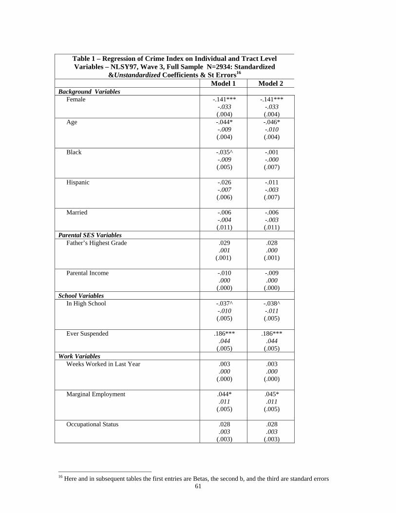
61

Table 1 – Regression of Crime Index on Individual and Tract Level Variables – NLSY97, Wave 3, Full Sample N=2934: Standardized

&Unstandardized Coefficients & St Errors16

Model 1 Model 2 Background Variables Female

-.141*** -.033 (.004)

-.141*** -.033 (.004)

Age

-.044* -.009 (.004)

-.046* -.010 (.004)

Black

-.035^ -.009 (.005)

-.001 -.000 (.007)

Hispanic

-.026 -.007 (.006)

-.011 -.003 (.007)

Married

-.006 -.004 (.011)

-.006 -.003 (.011)

Parental SES Variables Father’s Highest Grade

.029

.001 (.001)

.028

.000 (.001)

Parental Income

-.010 .000

(.000)

-.009 .000

(.000) School Variables In High School

-.037^ -.010 (.005)

-.038^ -.011 (.005)

Ever Suspended

.186*** .044

(.005)

.186*** .044

(.005) Work Variables Weeks Worked in Last Year

.003

.000 (.000)

.003

.000 (.000)

Marginal Employment

.044* .011

(.005)

.045* .011

(.005)

Occupational Status

.028

.003 (.003)

.028

.003 (.003)

16 Here and in subsequent tables the first entries are Betas, the second b, and the third are standard errors

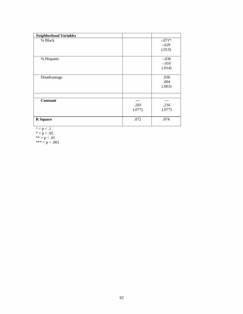
62

Neighborhood Variables % Black

-.071* -.029 (.013)

% Hispanic -.030

-.016 (.014)

Disadvantage

.036 .004

(.003)

Constant

--- .203

(.077)

--- .216

(.077)

R Square

.072 .074

^ = p < .1 * = p < .05 ** = p < .01 *** = p < .001

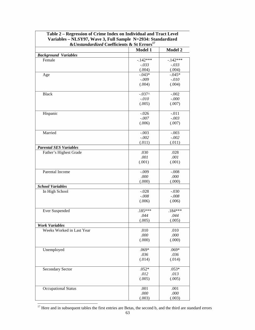
63

Table 2 – Regression of Crime Index on Individual and Tract Level Variables – NLSY97, Wave 3, Full Sample N=2934: Standardized

&Unstandardized Coefficients & St Errors17

Model 1 Model 2 Background Variables Female

-.142*** -.033 (.004)

-.142*** -.033 (.004)

Age

-.043* -.009 (.004)

-.045* -.010 (.004)

Black

-.037^ -.010 (.005)

-.002 -.000 (.007)

Hispanic

-.026 -.007 (.006)

-.011 -.003 (.007)

Married

-.003 -.002 (.011)

-.003 -.002 (.011)

Parental SES Variables Father’s Highest Grade

.030

.001 (.001)

.028

.001 (.001)

Parental Income

-.009 .000

(.000)

-.008 .000

(.000) School Variables In High School

-.028 -.008 (.006)

-.030 -.008 (.006)

Ever Suspended

.185*** .044

(.005)

.184*** .044

(.005) Work Variables Weeks Worked in Last Year

.010

.000 (.000)

.010

.000 (.000)

Unemployed

.069* .036

(.014)

.069* .036

(.014)

Secondary Sector

.052* .012

(.005)

.053* .013

(.005)

Occupational Status

.001

.000 (.003)

.001

.000 (.003)

17 Here and in subsequent tables the first entries are Betas, the second b, and the third are standard errors

64

Neighborhood Variables % Black

-.071* -.029 (.013)

% Hispanic -.031

-.017 (.014)

Disadvantage

.035 .004

(.003)

Constant

--- .208

(.077)

--- .221

(.077)

R Square

.074 .076

^ = p < .1 * = p < .05 ** = p < .01 *** = p < .001

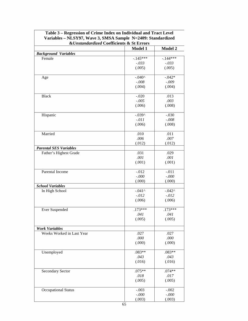
65

Table 3 – Regression of Crime Index on Individual and Tract Level Variables – NLSY97, Wave 3, SMSA Sample N=2409: Standardized

&Unstandardized Coefficients & St Errors Model 1 Model 2

Background Variables Female

-.145*** -.033 (.005)

-.144*** -.033 (.005)

Age

-.040^ -.008 (.004)

-.042* -.009 (.004)

Black

-.020 -.005 (.006)

.013

.003 (.008)

Hispanic

-.039^ -.011 (.006)

-.030 -.008 (.008)

Married

.010

.006 (.012)

.011

.007 (.012)

Parental SES Variables Father’s Highest Grade

.031

.001 (.001)

.029

.001 (.001)

Parental Income

-.012 -.000 (.000)

-.011 -.000 (.000)

School Variables In High School

-.041^ -.012 (.006)

-.042^ -.012 (.006)

Ever Suspended

.173*** .041

(.005)

.173*** .041

(.005)

Work Variables Weeks Worked in Last Year

.027

.000 (.000)

.027

.000 (.000)

Unemployed

.083** .043

(.016)

.083** .043

(.016)

Secondary Sector

.075** .018

(.005)

.074** .017

(.005)

Occupational Status

-.003 -.000 (.003)

-.002 -.000 (.003)

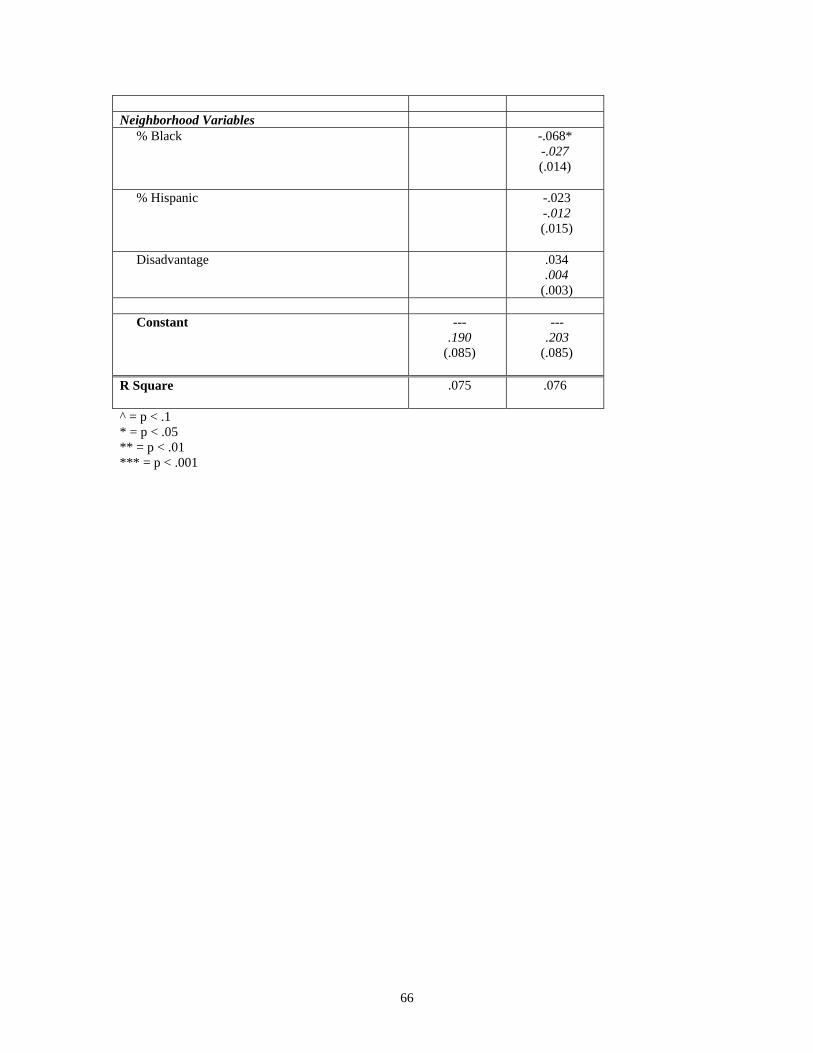
66

Neighborhood Variables % Black

-.068* -.027 (.014)

% Hispanic -.023

-.012 (.015)

Disadvantage

.034 .004

(.003) Constant

--- .190

(.085)

--- .203

(.085)

R Square

.075 .076

^ = p < .1 * = p < .05 ** = p < .01 *** = p < .001

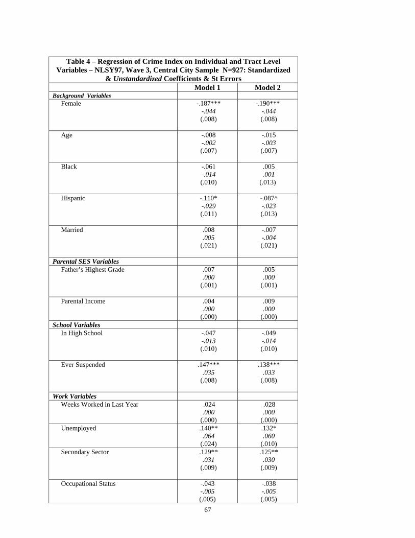
67

Table 4 – Regression of Crime Index on Individual and Tract Level

Variables – NLSY97, Wave 3, Central City Sample N=927: Standardized & Unstandardized Coefficients & St Errors

Model 1 Model 2 Background Variables Female

-.187*** -.044 (.008)

-.190*** -.044 (.008)

Age

-.008 -.002 (.007)

-.015 -.003 (.007)

Black

-.061 -.014 (.010)

.005

.001 (.013)

Hispanic

-.110* -.029 (.011)

-.087^ -.023 (.013)

Married

.008

.005 (.021)

-.007 -.004 (.021)

Parental SES Variables Father’s Highest Grade

.007

.000 (.001)

.005

.000 (.001)

Parental Income

.004

.000 (.000)

.009

.000 (.000)

School Variables In High School

-.047 -.013 (.010)

-.049 -.014 (.010)

Ever Suspended

.147*** .035

(.008)

.138*** .033

(.008)

Work Variables Weeks Worked in Last Year .024

.000 (.000)

.028 .000

(.000) Unemployed

.140** .064

(.024)

.132* .060

(.010) Secondary Sector

.129** .031

(.009)

.125** .030

(.009)

Occupational Status

-.043 -.005 (.005)

-.038 -.005 (.005)

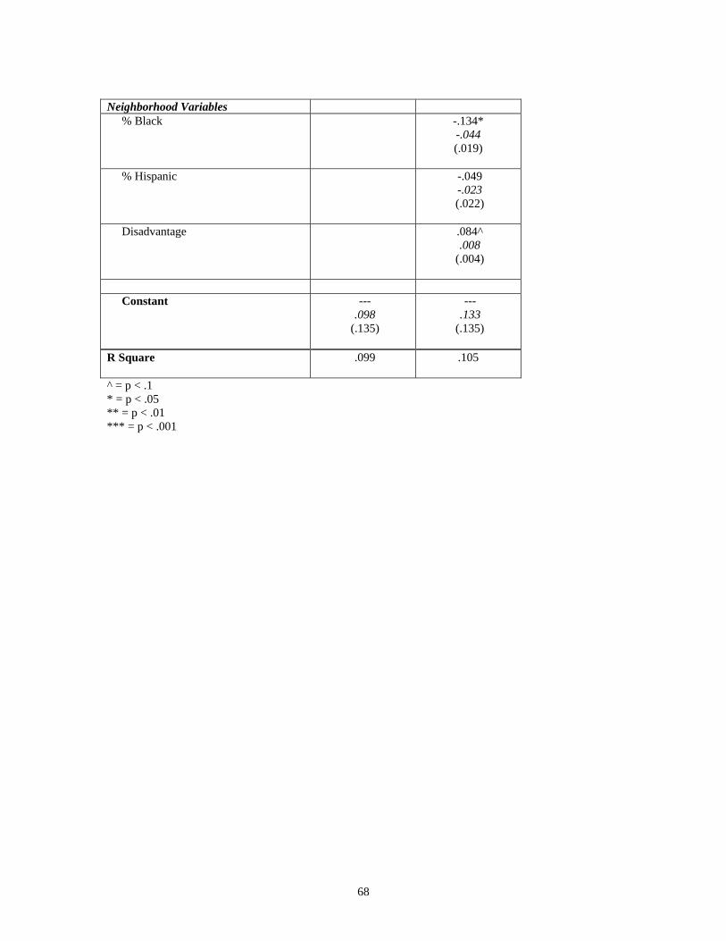
68

Neighborhood Variables % Black

-.134* -.044 (.019)

% Hispanic -.049

-.023 (.022)

Disadvantage

.084^ .008

(.004)

Constant

--- .098

(.135)

--- .133

(.135)

R Square

.099 .105

^ = p < .1 * = p < .05 ** = p < .01 *** = p < .001

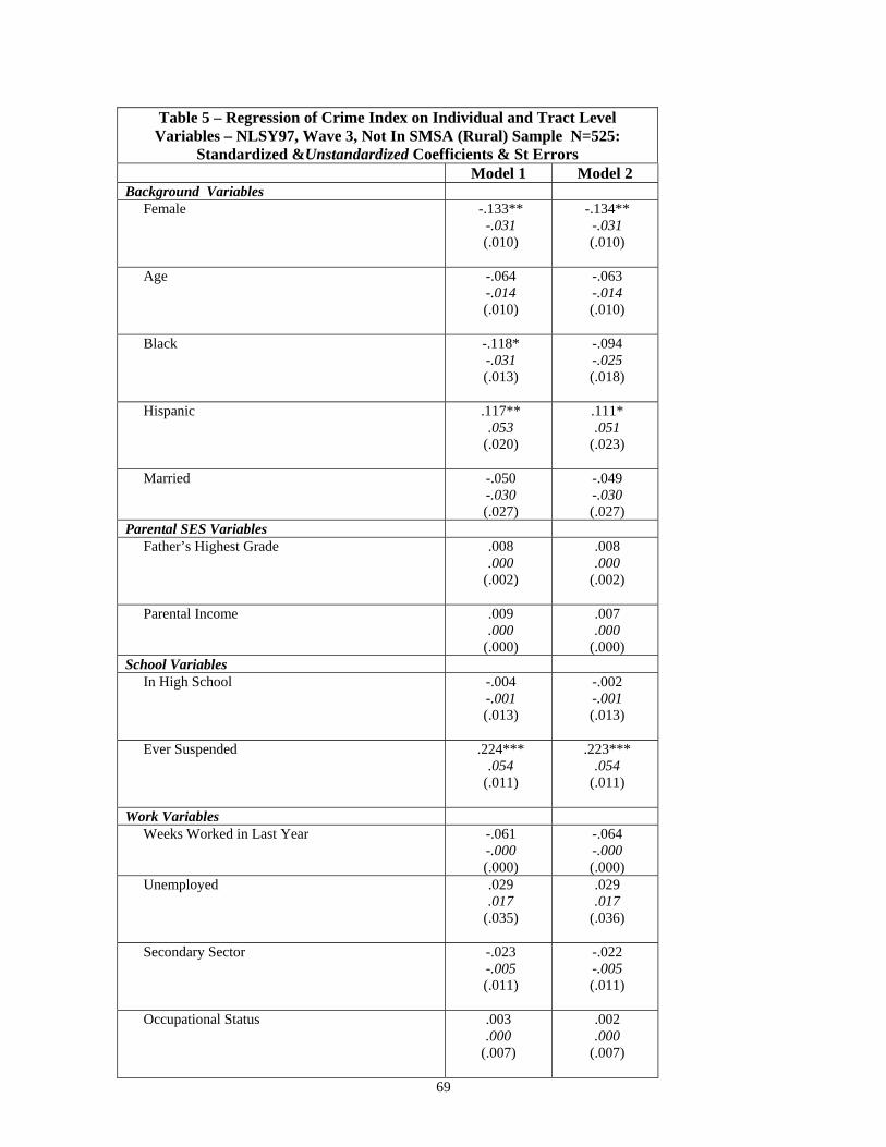
69

Table 5 – Regression of Crime Index on Individual and Tract Level Variables – NLSY97, Wave 3, Not In SMSA (Rural) Sample N=525:

Standardized &Unstandardized Coefficients & St Errors Model 1 Model 2

Background Variables Female

-.133** -.031 (.010)

-.134** -.031 (.010)

Age

-.064 -.014 (.010)

-.063 -.014 (.010)

Black

-.118* -.031 (.013)

-.094 -.025 (.018)

Hispanic

.117** .053

(.020)

.111* .051

(.023)

Married

-.050 -.030 (.027)

-.049 -.030 (.027)

Parental SES Variables Father’s Highest Grade

.008

.000 (.002)

.008

.000 (.002)

Parental Income

.009

.000 (.000)

.007

.000 (.000)

School Variables In High School

-.004 -.001 (.013)

-.002 -.001 (.013)

Ever Suspended

.224*** .054

(.011)

.223*** .054

(.011)

Work Variables Weeks Worked in Last Year

-.061 -.000 (.000)

-.064 -.000 (.000)

Unemployed

.029

.017 (.035)

.029

.017 (.036)

Secondary Sector

-.023 -.005 (.011)

-.022 -.005 (.011)

Occupational Status

.003

.000 (.007)

.002

.000 (.007)

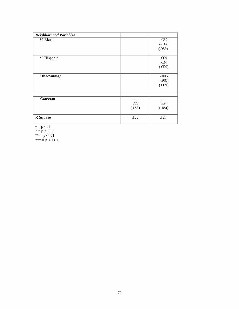
70

Neighborhood Variables % Black

-.030 -.014 (.039)

% Hispanic .009

.010 (.056)

Disadvantage

-.005 -.001 (.009)

Constant

--- .322

(.183)

--- .320

(.184)

R Square

.122 .123

^ = p < .1 * = p < .05 ** = p < .01 *** = p < .001

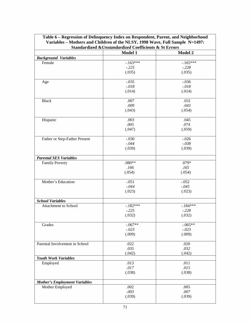
71

Table 6 – Regression of Delinquency Index on Respondent, Parent, and Neighborhood

Variables – Mothers and Children of the NLSY, 1998 Wave, Full Sample N=1497: Standardized &Unstandardized Coefficients & St Errors

Model 1 Model 2 Background Variables Female

-.163*** -.225 (.035)

-.165*** -.228 (.035)

Age

-.035 -.018 (.014)

-.036 -.018 (.014)

Black

.007 .009 (.043)

.031 .043 (.054)

Hispanic

.003 .005

(.047)

.045 .074

(.059)

Father or Step-Father Present -.030 -.044 (.039)

-.026 -.038 (.039)

Parental SES Variables Family Poverty

.080** .166

(.054)

.079* .165

(.054)

Mother’s Education

-.051 -.044

(.023)

-.052 -.045

(.023)

School Variables Attachment to School

-.182*** -.225 (.032)

-.184*** -.228 (.032)

Grades

-.067** -.023 (.009)

-.065** -.023 (.009)

Parental Involvement in School

.022

.035 (.042)

.020

.032 (.042)

Youth Work Variables Employed

.013

.017 (.038)

.011

.015 (.038)

Mother’s Employment Variables Mother Employed

.002

.003 (.039)

.005

.007 (.039)

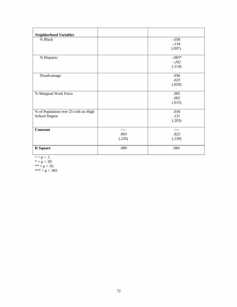
72

Neighborhood Variables

% Black

-.058 -.134 (.097)

% Hispanic -.083*

-.262 (.114)

Disadvantage

.036 .023

(.029)

% Marginal Work Force

.005 .002

(.015)

% of Population over 25 with no High School Degree

.018 .131

(.203)

Constant

---- .803

(.226)

---- .822

(.228)

R Square

.080 .084

^ = p < .1 * = p < .05 ** = p < .01 *** = p < .001

73

Table 7 – Regression of Delinquency Index on Respondent, Parent, and Neighborhood

Variables – Mothers and Children of the NLSY, 1998 Wave, In SMSA Sample N=1167: Standardized &Unstandardized Coefficients & St Errors

Model 1 Model 2 Background Variables Female

-.150*** -.203 (.039)

-.154*** -.209 (.039)

Age

-.025 -.013 (.016)

-.024 -.012 (.015)

Black

.002 .003 (.049)

.049 .068 (.059)

Hispanic

-.008 -.013 (.051)

.042 .065

(.064)

Father or Step-Father Present -.065 * -.092 (.043)

-.058^ -.083 (.044)

Parental SES Variables Family Poverty

.065* .127

(.059)

.063* .123

(.059)

Mother’s Education

-.051^ -.043

(.025)

-.055^ -.042

(.026)

School Variables Attachment to School

-.157*** -.194 (.037)

-.159*** -.197 (.037)

Grades

-.048 -.016 (.010)

-.045 -.015 (.010)

Parental Involvement in School

.007

.011 (.047)

.004

.006 (.047)

Youth Work Variables Employed

.031

.043 (.042)

.019

.069 (.043)

Mother’s Employment Variables Mother Employed

.008

.012 (.044)

.012

.018 (.044)

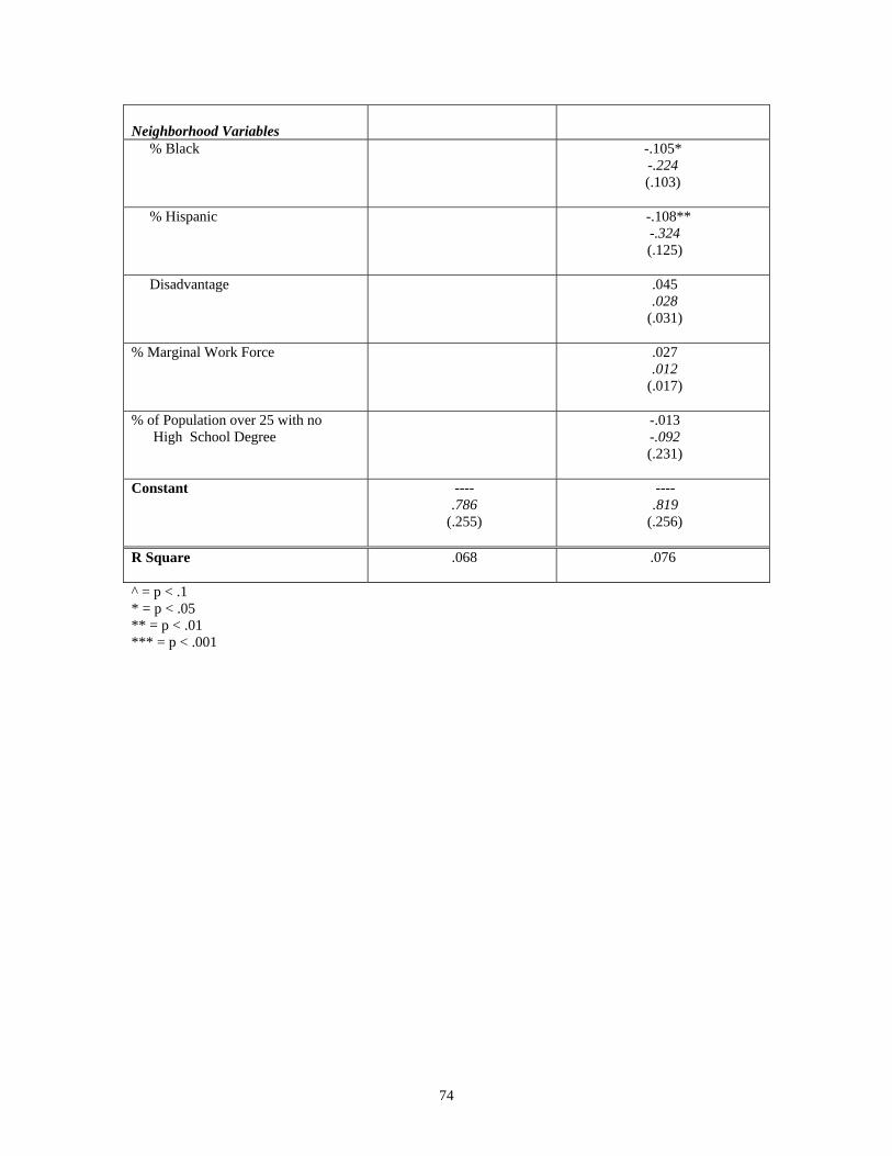
74

Neighborhood Variables

% Black

-.105* -.224 (.103)

% Hispanic -.108**

-.324 (.125)

Disadvantage

.045 .028

(.031)

% Marginal Work Force

.027 .012

(.017)

% of Population over 25 with no High School Degree

-.013 -.092 (.231)

Constant

---- .786

(.255)

---- .819

(.256)

R Square

.068 .076

^ = p < .1 * = p < .05 ** = p < .01 *** = p < .001

75

Table 8 – Regression of Delinquency Index on Respondent, Parent, and Neighborhood

Variables – Mothers and Children of the NLSY, 1998 Wave, Central City Sample N=475: Standardized &Unstandardized Coefficients & St Errors

Model 1 Model 2 Background Variables Female

-.163*** -.232 (.065)

-.173*** -.247 (.065)

Age

-.045 -..023 (.026)

-.046 -.024 (.026)

Black

-.036 -.052 (.089)

.025 .036 (.107)

Hispanic

.009 .014

(.098)

.089 .143

(.118)

Father or Step-Father Present -.102 -.147 (.069)

-.090 -.130 (.070)

Parental SES Variables Family Poverty

.076

.145 (.091)

.071 .103

(.093)

Mother’s Education

-.024 - .021

(.041)

-.024 - .021

(.042)

School Variables Attachment to School

-.129** -.169 (.062)

-.136** -.178 (.062)

Grades

-.031 -.011 (.016)

-.024 -.008 (.016)

Parental Involvement in School

.042 .067 (.078)

.032 .051 (.079)

Youth Work Variables Employed

.097^ .138

(.071)

.087^ .125

(.073)

Mother’s Employment Variables Mother Employed

.027

.041 (.072)

.034

.052 (.073)

76

Neighborhood Variables

% Black

-.138^ -.265 (.146)

% Hispanic -.157*

-.467 (.198)

Disadvantage

.093 .049

(.042)

% Marginal Work Force

-.025 -.011 (.030)

% of Population over 25 with no High School Degree

.026 .169

(.339)

Constant

---- .967

(.424)

---- 1.013 (.427)

R Square

.073 .087

^ = p < .1 * = p < .05 ** = p < .01 *** = p < .001

77

Table 9 – Regression of Delinquency Index on Respondent, Parent, and Neighborhood

Variables – Mothers and Children of the NLSY, 1998 Wave, Rural Sample N=330: Standardized &Unstandardized Coefficients & St Errors

Model 1 Model 2 Background Variables Female

-.166** -.241 (.078)

-.172** -.249 (.079)

Age

-.056 -.029 (.030)

-.059 -.031 (.030)

Black

.016 .025 (.104)

- .104 -.163 (.142)

Hispanic

.016 .035

(.120)

.054 .120

(.155)

Father or Step-Father Present .085 .133

(.096)

.082

.127 (.096)

Parental SES Variables Family Poverty

.159** 4265

(.144)

.158* .425

(.145)

Mother’s Education

-.069 -.067

(.053)

-.064 -.062

(.058)

School Variables Attachment to School

-.276*** -.342 (.067)

-.284** -.351 (.068)

Grades

-.118* -.047 (.022)

-.114* -.046 (.022)

Parental Involvement in School

.065

.111 (.092)

.065

.109 (.093)

Youth Work Variables Employed

-.047 -.068 (.084)

-.041 -.059 (.085)

Mother’s Employment Variables Mother Employed

.003

.004 (.084)

.005

.008 (.084)

78

Neighborhood Variables

% Black

.149 .506

(.326)

% Hispanic -.047 -.198 (.325)

Disadvantage

.005 .004

(.092)

% Marginal Work Force

-.024 -.014 (.043)

% of Population over 25 with no High School Degree

.02834 .203

(.445)

Constant

---- .753

(.495)

---- .738

(.507)

R Square

.166 .177

^ = p < .1 * = p < .05 ** = p < .01 *** = p < .001

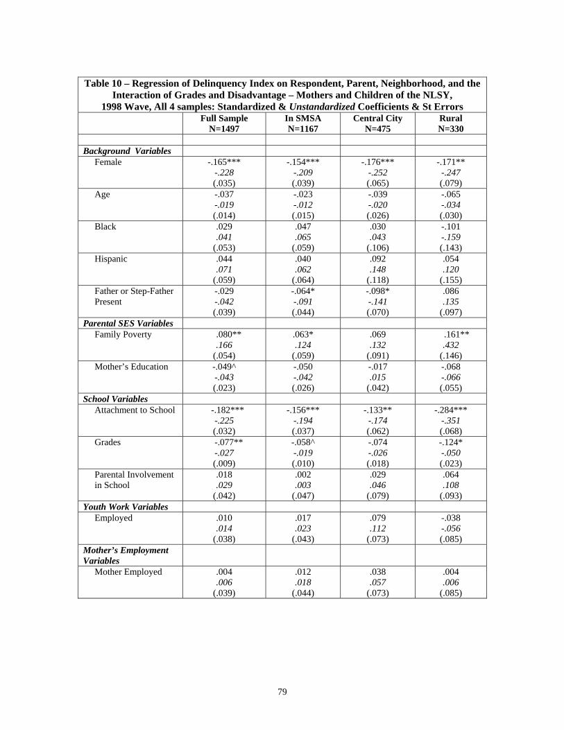
79

Table 10 – Regression of Delinquency Index on Respondent, Parent, Neighborhood, and the

Interaction of Grades and Disadvantage – Mothers and Children of the NLSY, 1998 Wave, All 4 samples: Standardized & Unstandardized Coefficients & St Errors

Full Sample N=1497

In SMSA N=1167

Central City N=475

Rural N=330

Background Variables Female

-.165*** -.228 (.035)

-.154*** -.209 (.039)

-.176*** -.252 (.065)

-.171** -.247 (.079)

Age

-.037 -.019 (.014)

-.023 -.012 (.015)

-.039 -.020 (.026)

-.065 -.034 (.030)

Black

.029

.041 (.053)

.047

.065 (.059)

.030

.043 (.106)

-.101 -.159 (.143)

Hispanic

.044

.071 (.059)

.040

.062 (.064)

.092

.148 (.118)

.054

.120 (.155)

Father or Step-Father Present

-.029 -.042 (.039)

-.064* -.091 (.044)

-.098* -.141 (.070)

.086

.135 (.097)

Parental SES Variables Family Poverty

.080** .166

(.054)

.063* .124

(.059)

.069

.132 (.091)

.161** .432

(.146) Mother’s Education

-.049^ -.043 (.023)

-.050 -.042 (.026)

-.017 .015

(.042)

-.068 -.066 (.055)

School Variables Attachment to School

-.182*** -.225 (.032)

-.156*** -.194 (.037)

-.133** -.174 (.062)

-.284*** -.351 (.068)

Grades

-.077** -.027 (.009)

-.058^ -.019 (.010)

-.074 -.026 (.018)

-.124* -.050 (.023)

Parental Involvement in School

.018

.029 (.042)

.002

.003 (.047)

.029

.046 (.079)

.064

.108 (.093)

Youth Work Variables Employed

.010

.014 (.038)

.017

.023 (.043)

.079

.112 (.073)

-.038 -.056 (.085)

Mother’s Employment Variables

Mother Employed

.004

.006 (.039)

.012

.018 (.044)

.038

.057 (.073)

.004

.006 (.085)

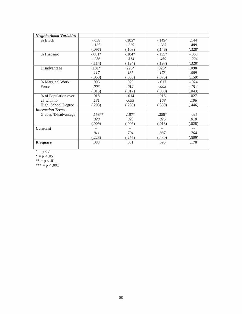
80

Neighborhood Variables % Black

-.058 -.135 (.097)

-.105* -.225 (.103)

-.149^ -.285 (.146)

.144

.489 (.328)

% Hispanic

-.081* -.256 (.114)

-.104* -.314 (.124)

-.155* -.459 (.197)

-.053 -.224 (.328)

Disadvantage

.181* .117

(.050)

.225* .135

(.053)

.328* .173

(.075)

.098

.089 (.159)

% Marginal Work Force

.006

.003 (.015)

.029

.012 (.017)

-.017 -.008 (.030)

-.024 -.014 (.043)

% of Population over 25 with no High School Degree

.018

.131 (.203)

-.014 -.095 (.230)

.016

.108 (.339)

.027

.196 (.446)

Interaction Terms Grades*Disadvantage

.158** .020

(.009)

.197* .023

(.009)

.258* .026

(.013)

.095 .018

(.028) Constant

-- .811

(.228)

-- .794

(.256)

-- .887

(.430)

-- .764

(.509) R Square

.088 .081 .095 .178

^ = p < .1 * = p < .05 ** = p < .01 *** = p < .001

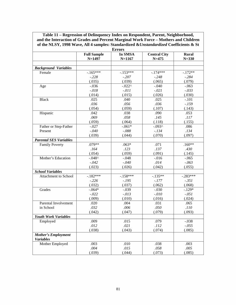
81

Table 11 – Regression of Delinquency Index on Respondent, Parent, Neighborhood,

and the Interaction of Grades and Percent Marginal Work Force – Mothers and Children of the NLSY, 1998 Wave, All 4 samples: Standardized &Unstandardized Coefficients & St

Errors Full Sample

N=1497 In SMSA N=1167

Central City N=475

Rural N=330

Background Variables Female

-.165*** -.228 (.035)

-.153*** -.207 (.039)

-.174*** -.248 (.065)

-.172** -.284 (.079)

Age

-.036 -.018 (.014)

-.022^ -.011 (.015)

-.040 -.021 (.026)

-.063 -.033 (.030)

Black

.025

.036 (.054)

.040

.056 (.059)

.025

.036 (.107)

-.101 -.159 (.143)

Hispanic

.042

.069 (.059)

.038

.058 (.064)

.090

.145 (.118)

.053

.117 (.155)

Father or Step-Father Present

-.027 -.040 (.039)

-.061* -.088 (.044)

-.093^ -.134 (.070)

.086

.134 (.097)

Parental SES Variables Family Poverty

.079** .164

(.054)

.063* .123

(.059)

.071

.137 (.091)

.160** .430

(.145) Mother’s Education

-.048^ -.042 (.023)

-.048 -.040 (.026)

-.016 .014

(.042)

-.065 -.063 (.055)

School Variables Attachment to School

-.182*** -.226 (.032)

-.158*** -.195 (.037)

-.135** -.177 (.062)

-.283*** -.351 (.068)

Grades

-.064* -.022 (.009)

-.039 -.013 (.010)

-.030 -.010 (.016)

-.129* -.051 (.024)

Parental Involvement in School

.020

.032 (.042)

.004

.006 (.047)

.031

.050 (.079)

.065

.110 (.093)

Youth Work Variables Employed

.009

.012 (.038)

.015

.021 (.043)

.079

.112 (.074)

-.038 -.055 (.085)

Mother’s Employment Variables

Mother Employed

.003

.004 (.039)

.010

.015 (.044)

.038

.058 (.073)

.003

.005 (.085)

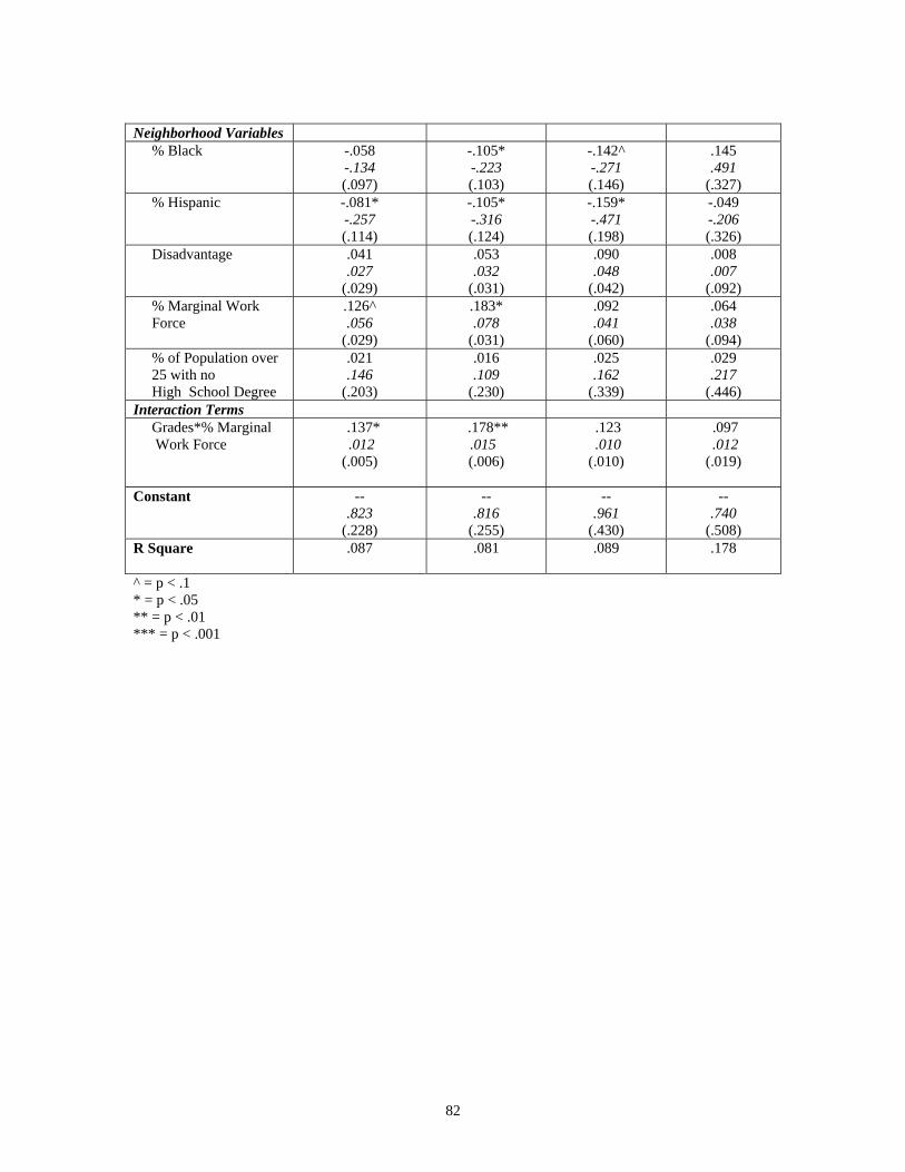
82

Neighborhood Variables % Black

-.058 -.134 (.097)

-.105* -.223 (.103)

-.142^ -.271 (.146)

.145

.491 (.327)

% Hispanic

-.081* -.257 (.114)

-.105* -.316 (.124)

-.159* -.471 (.198)

-.049 -.206 (.326)

Disadvantage

.041

.027 (.029)

.053

.032 (.031)

.090

.048 (.042)

.008

.007 (.092)

% Marginal Work Force

.126^ .056

(.029)

.183* .078

(.031)

.092

.041 (.060)

.064

.038 (.094)

% of Population over 25 with no High School Degree

.021

.146 (.203)

.016

.109 (.230)

.025

.162 (.339)

.029

.217 (.446)

Interaction Terms Grades*% Marginal Work Force

.137* .012 (.005)

.178** .015 (.006)

.123 .010 (.010)

.097 .012 (.019)

Constant

-- .823

(.228)

-- .816

(.255)

-- .961

(.430)

-- .740

(.508) R Square

.087 .081 .089 .178

^ = p < .1 * = p < .05 ** = p < .01 *** = p < .001

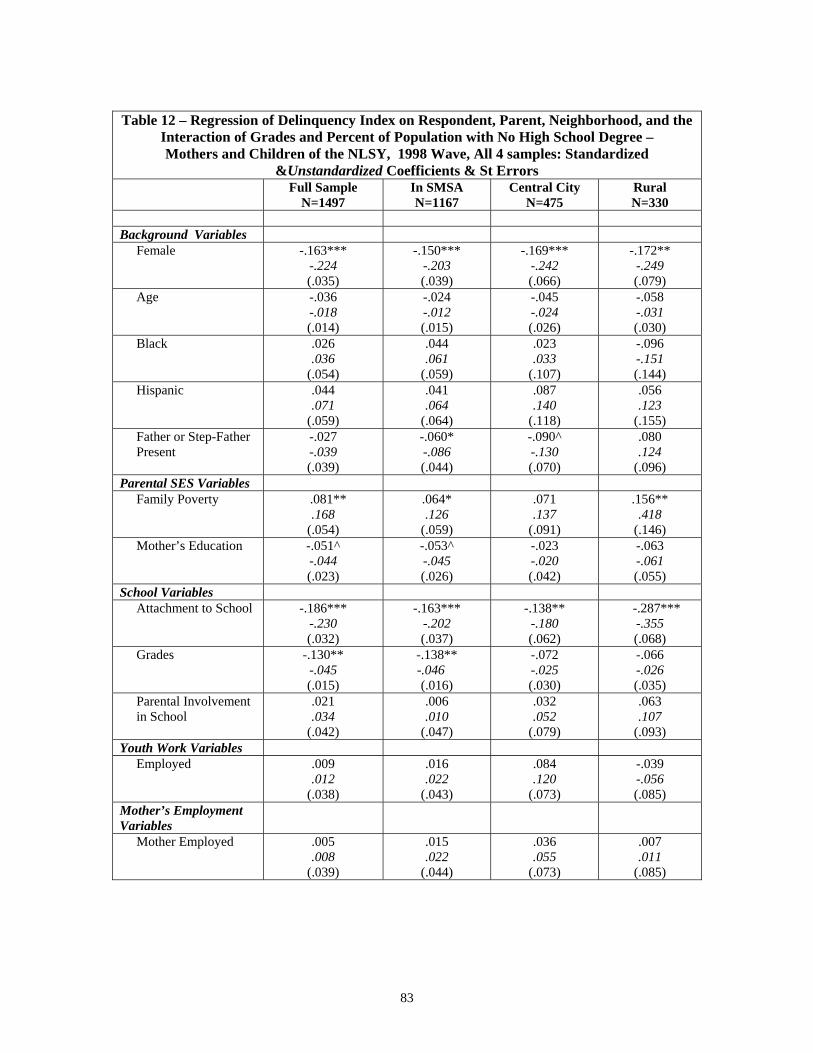
83

Table 12 – Regression of Delinquency Index on Respondent, Parent, Neighborhood, and the

Interaction of Grades and Percent of Population with No High School Degree – Mothers and Children of the NLSY, 1998 Wave, All 4 samples: Standardized

&Unstandardized Coefficients & St Errors Full Sample

N=1497 In SMSA N=1167

Central City N=475

Rural N=330

Background Variables Female

-.163*** -.224 (.035)

-.150*** -.203 (.039)

-.169*** -.242 (.066)

-.172** -.249 (.079)

Age

-.036 -.018 (.014)

-.024 -.012 (.015)

-.045 -.024 (.026)

-.058 -.031 (.030)

Black

.026

.036 (.054)

.044

.061 (.059)

.023

.033 (.107)

-.096 -.151 (.144)

Hispanic

.044

.071 (.059)

.041

.064 (.064)

.087

.140 (.118)

.056

.123 (.155)

Father or Step-Father Present

-.027 -.039 (.039)

-.060* -.086 (.044)

-.090^ -.130 (.070)

.080

.124 (.096)

Parental SES Variables Family Poverty

.081** .168

(.054)

.064* .126

(.059)

.071

.137 (.091)

.156** .418

(.146) Mother’s Education

-.051^ -.044 (.023)

-.053^ -.045 (.026)

-.023 -.020 (.042)

-.063 -.061 (.055)

School Variables Attachment to School

-.186*** -.230 (.032)

-.163*** -.202 (.037)

-.138** -.180 (.062)

-.287*** -.355 (.068)

Grades

-.130** -.045 (.015)

-.138** -.046

(.016)

-.072 -.025 (.030)

-.066 -.026 (.035)

Parental Involvement in School

.021

.034 (.042)

.006

.010 (.047)

.032

.052 (.079)

.063

.107 (.093)

Youth Work Variables Employed

.009

.012 (.038)

.016

.022 (.043)

.084

.120 (.073)

-.039 -.056 (.085)

Mother’s Employment Variables

Mother Employed

.005

.008 (.039)

.015

.022 (.044)

.036

.055 (.073)

.007

.011 (.085)

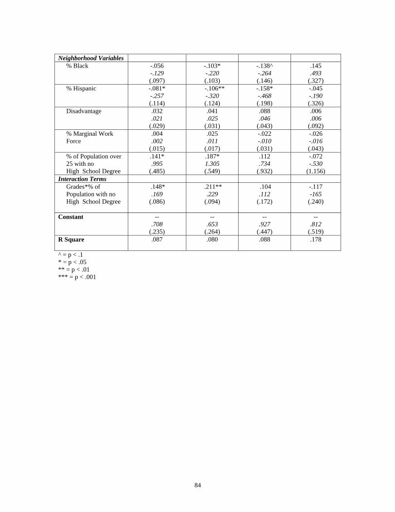
84

Neighborhood Variables % Black

-.056 -.129 (.097)

-.103* -.220 (.103)

-.138^ -.264 (.146)

.145

.493 (.327)

% Hispanic

-.081* -.257 (.114)

-.106** -.320 (.124)

-.158* -.468 (.198)

-.045 -.190 (.326)

Disadvantage

.032

.021 (.029)

.041

.025 (.031)

.088

.046 (.043)

.006

.006 (.092)

% Marginal Work Force

.004

.002 (.015)

.025

.011 (.017)

-.022 -.010 (.031)

-.026 -.016 (.043)

% of Population over 25 with no High School Degree

.141* .995

(.485)

.187* 1.305 (.549)

.112

.734 (.932)

-.072 -.530

(1.156) Interaction Terms Grades*% of Population with no High School Degree

.148* .169

(.086)

.211** .229

(.094)

.104 .112

(.172)

-.117 -165

(.240)

Constant

-- .708

(.235)

-- .653

(.264)

-- .927

(.447)

-- .812

(.519) R Square

.087 .080 .088 .178

^ = p < .1 * = p < .05 ** = p < .01 *** = p < .001

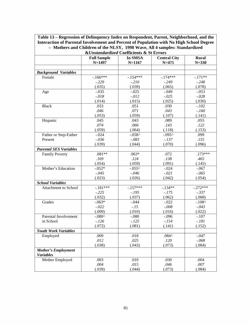
85

Table 13 – Regression of Delinquency Index on Respondent, Parent, Neighborhood, and the Interaction of Parental Involvement and Percent of Population with No High School Degree

– Mothers and Children of the NLSY, 1998 Wave, All 4 samples: Standardized &Unstandardized Coefficients & St Errors

Full Sample N=1497

In SMSA N=1167

Central City N=475

Rural N=330

Background Variables Female

-.166*** -.229 (.035)

-.154*** -.210 (.039)

-.174*** -.249 (.065)

-.171** -.248 (.078)

Age

-.035 -.018 (.014)

-.025 -.012 (.015)

-.049 -.025 (.025)

-.053 -.028 (.030)

Black

.033

.046 (.053)

.051

.071 (.059)

.030

.043 (.107)

-.102 -.160 (.141)

Hispanic

.045

.074 (.059)

.043

.066 (.064)

.089

.143 (.118)

.055

.122 (.153)

Father or Step-Father Present

-.024 -.036 (.039)

-.058^ -.083 (.044)

-.095^ -.137 (.070)

.099

.155 (.096)

Parental SES Variables Family Poverty

.081** .169

(.054)

.063* .124

(.059)

.072

.138 (.091)

.173*** .465

(.145) Mother’s Education

-.052* -.045 (.023)

-.055^ -.046 (.026)

-.024 -.021 (.042)

-.067 -.065 (.054)

School Variables Attachment to School

-.181*** -.225 (.032)

-.157*** -.195 (.037)

-.134** -.175 (.062)

-.272*** -.337 (.068)

Grades

-.063* -.022 (.009)

-.044 -.15

(.010)

-.022 -.008 (.016)

-.108^ -.043 (.022)

Parental Involvement in School

-.080^ -.126 (.072)

-.080 -.125 (.081)

-.096 -.154 (.141)

-.107 -.181 (.152)

Youth Work Variables Employed

.009

.012 (.038)

.018

.025 (.043)

.084^ .120

(.073)

-.047 -.068 (.084)

Mother’s Employment Variables

Mother Employed

.003

.004 (.039)

.010

.015 (.044)

.030

.046 (.073)

.004

.007 (.084)

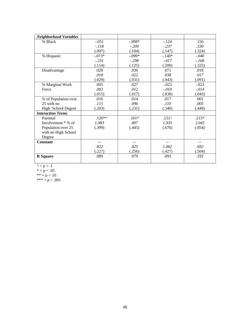
86

Neighborhood Variables % Black

-.051 -.118 (.097)

-.098* -.209 (.104)

-.124 -.237 (.147)

.156

.530 (.324)

% Hispanic

-.073* -.231 (.114)

-.099* -.298 (.125)

-.140* -.417 (.200)

-.040 -.168 (.323)

Disadvantage

.028

.018 (.029)

.036

.022 (.031)

.071

.038 (.043)

.018

.017 (.091)

% Marginal Work Force

.005

.002 (.015)

.027

.012 (.017)

-.023 -.010 (.030)

-.023 -.014 (.043)

% of Population over 25 with no High School Degree

.016

.115 (.203)

.014

.096 (.231)

.017

.110 (.340)

.001

.005 (.449)

Interaction Terms Parental Involvement * % of Population over 25 with no High School Degree

.120** 1.083 (.399)

.101* .897

(.445)

.151^ 1.935 (.676)

.215* 2.045 (.854)

Constant

-- .822

(.227)

-- .825

(.256)

-- 1.062 (.427)

-- .692

(.504) R Square

.089 .079 .093 .192

^ = p < .1 * = p < .05 ** = p < .01 *** = p < .001

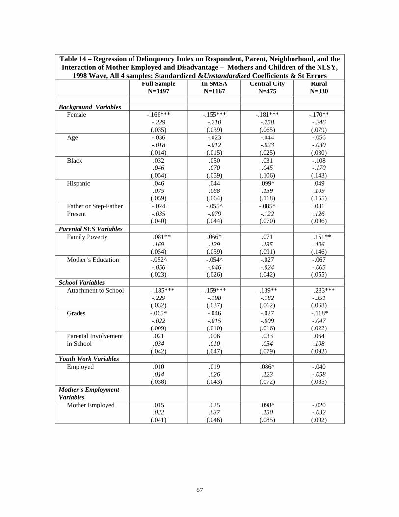
87

Table 14 – Regression of Delinquency Index on Respondent, Parent, Neighborhood, and the Interaction of Mother Employed and Disadvantage – Mothers and Children of the NLSY,

1998 Wave, All 4 samples: Standardized &Unstandardized Coefficients & St Errors Full Sample

N=1497 In SMSA N=1167

Central City N=475

Rural N=330

Background Variables Female

-.166*** -.229 (.035)

-.155*** -.210 (.039)

-.181*** -.258 (.065)

-.170** -.246 (.079)

Age

-.036 -.018 (.014)

-.023 -.012 (.015)

-.044 -.023 (.025)

-.056 -.030 (.030)

Black

.032

.046 (.054)

.050

.070 (.059)

.031

.045 (.106)

-.108 -.170 (.143)

Hispanic

.046

.075 (.059)

.044

.068 (.064)

.099^ .159

(.118)

.049

.109 (.155)

Father or Step-Father Present

-.024 -.035 (.040)

-.055^ -.079 (.044)

-.085^ -.122 (.070)

.081

.126 (.096)

Parental SES Variables Family Poverty

.081** .169

(.054)

.066* .129

(.059)

.071

.135 (.091)

.151** .406

(.146) Mother’s Education

-.052^ -.056 (.023)

-.054^ -.046 (.026)

-.027 -.024 (.042)

-.067 -.065 (.055)

School Variables Attachment to School

-.185*** -.229 (.032)

-.159*** -.198 (.037)

-.139** -.182 (.062)

-.283*** -.351 (.068)

Grades

-.065* -.022 (.009)

-.046 -.015 (.010)

-.027 -.009 (.016)

-.118* -.047 (.022)

Parental Involvement in School

.021

.034 (.042)

.006

.010 (.047)

.033

.054 (.079)

.064

.108 (.092)

Youth Work Variables Employed

.010

.014 (.038)

.019

.026 (.043)

.086^ .123

(.072)

-.040 -.058 (.085)

Mother’s Employment Variables

Mother Employed

.015

.022 (.041)

.025

.037 (.046)

.098^ .150

(.085)

-.020 -.032 (.092)

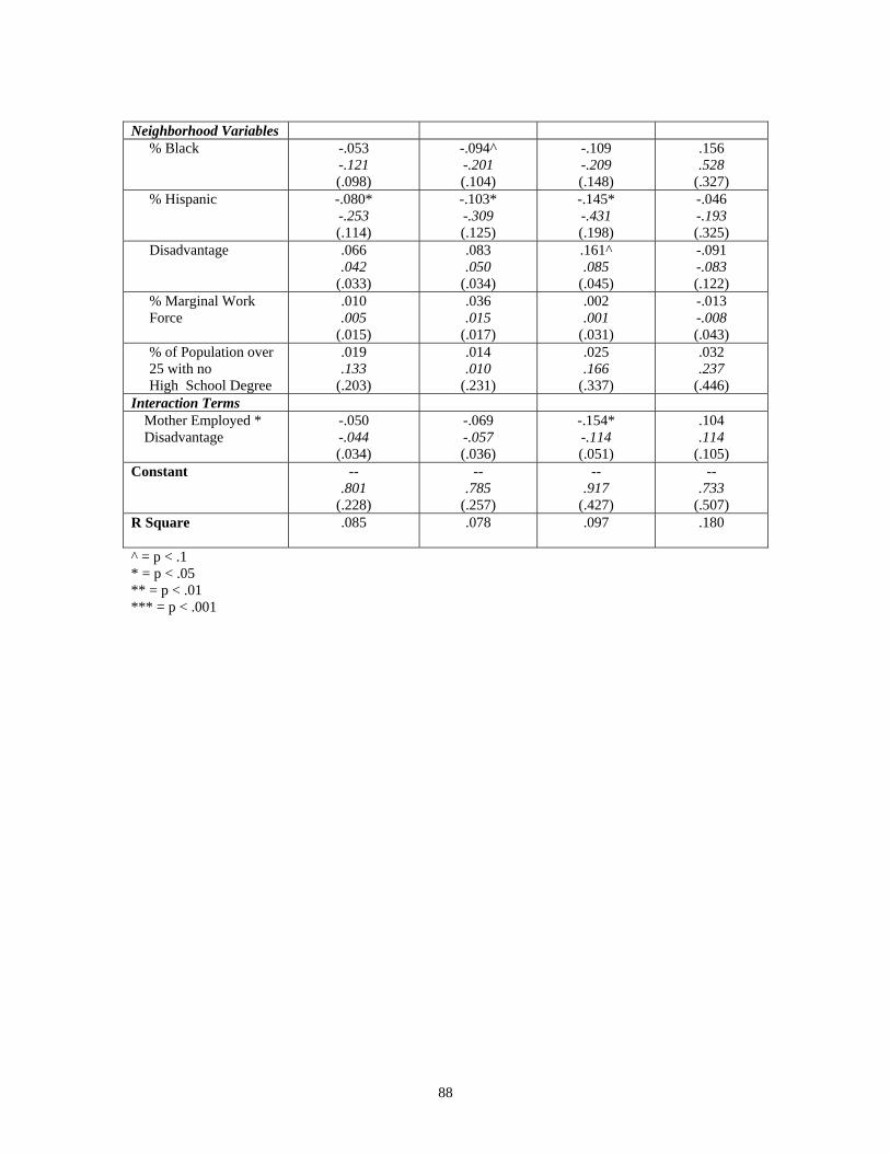
88

Neighborhood Variables % Black

-.053 -.121 (.098)

-.094^ -.201 (.104)

-.109 -.209 (.148)

.156

.528 (.327)

% Hispanic

-.080* -.253 (.114)

-.103* -.309 (.125)

-.145* -.431 (.198)

-.046 -.193 (.325)

Disadvantage

.066

.042 (.033)

.083

.050 (.034)

.161^ .085

(.045)

-.091 -.083 (.122)

% Marginal Work Force

.010

.005 (.015)

.036

.015 (.017)

.002

.001 (.031)

-.013 -.008 (.043)

% of Population over 25 with no High School Degree

.019

.133 (.203)

.014

.010 (.231)

.025

.166 (.337)

.032

.237 (.446)

Interaction Terms Mother Employed * Disadvantage

-.050 -.044 (.034)

-.069 -.057 (.036)

-.154* -.114 (.051)

.104

.114 (.105)

Constant

-- .801

(.228)

-- .785

(.257)

-- .917

(.427)

-- .733

(.507) R Square

.085 .078 .097 .180

^ = p < .1 * = p < .05 ** = p < .01 *** = p < .001

89

FIGURES HERE

90

93

Appendix A: Source Variables and Descriptions for All Variables in the Analyses

Variable Name

Source Variable

from NLSY97 Variable Description

Individual: Age R3876300 Age of Respondent at Interview Date Sex R3828700 Sex/Gender of Respondent. Recoded to 0=male, 1=female Race R1482600 Combined Race and Ethnicity of respondent.

Recoded to dummy variables indicating race: Black and Hispanic. Father’s Highest Grade R1302400 or

R1302500 Father’s Highest Grade Completed. Used biological father, or resident father if biological father was missing. Recoded the “ungraded” responses to the mean, and used mother’s education to estimate father’s if father’s was missing.

Father’s Highest Grade (flag for imputed data)

Created A dummy variable used in the analyses to indicate if father’s highest grade was imputed. 0=not imputed, 1=imputed.

Parental Income Sum of: R0492500 R0609800 R0610100 R0610500 R0610800 R0611100 R0611400 R0611700 R0612000 R0612400 R0612700

Our own created yearly income estimate consisting of a sum of the answers to the following 11 questions asked of the respondent’s parent on the parental retrospective questionnaire. 1. Total income received from rental property in 1996? 2. During 1996, how much income did you receive from wages, salary, commissions, or tips from all jobs, before deductions for taxes or anything else? 3. During 1996, how much income did you receive from your own farm, business, partnership or professional practice AFTER EXPENSES? 4. During 1996, how much income did your [spouse/partner] receive from wages, salary, commissions, or tips from all jobs, before deductions for taxes or anything else? 5. During 1996, how much did your [spouse/partner] receive from [his/her] own farm, business, partnership or professional practice AFTER EXPENSES? 6. What was the total amount of interest and dividend payments [you/you or your spouse/partner] received during 1996, including even small amounts and amounts reinvested or credited to the accounts? 7. What was the total amount of income [you/you and your spouse/partner] received from AFDC or ADC last year? 8. What was the total value of the food stamps [you/you and your spouse/partner] received during 1996? 9. What was the total amount [you/you and your spouse/partner] received from SSI? 10. How much did [you/you or your spouse/partner] receive in child-support during 1996? 11. What was the total amount [you/you and your spouse/partner] received from all other sources (e.g., friends, relatives, royalties or any other regular or periodic source of income) during 1996?

Parental Income (flag for imputed data)

Created A dummy variable used in the analyses to indicate if parent’s income was imputed. 0=not imputed, 1=imputed.

Enrollment in High School R3881500 Respondent’s enrollment in school. Recoded to 1=enrolled in grades 1-12. 0=not enrolled in school, or

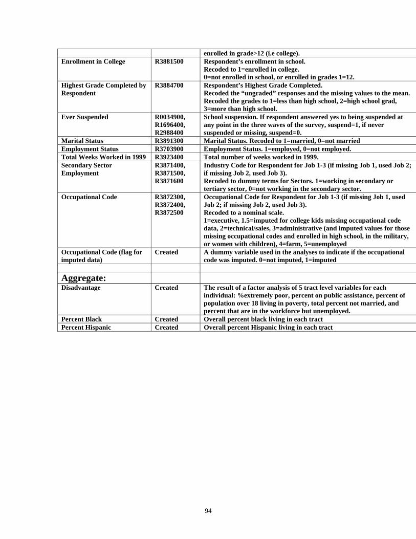
94

enrolled in grade>12 (i.e college). Enrollment in College R3881500 Respondent’s enrollment in school.

Recoded to 1=enrolled in college. 0=not enrolled in school, or enrolled in grades 1=12.

Highest Grade Completed by Respondent

R3884700 Respondent’s Highest Grade Completed. Recoded the “ungraded” responses and the missing values to the mean. Recoded the grades to 1=less than high school, 2=high school grad, 3=more than high school.

Ever Suspended R0034900, R1696400, R2988400

School suspension. If respondent answered yes to being suspended at any point in the three waves of the survey, suspend=1, if never suspended or missing, suspend=0.

Marital Status R3891300 Marital Status. Recoded to 1=married, 0=not married Employment Status R3703900 Employment Status. 1=employed, 0=not employed. Total Weeks Worked in 1999 R3923400 Total number of weeks worked in 1999. Secondary Sector Employment

R3871400, R3871500, R3871600

Industry Code for Respondent for Job 1-3 (if missing Job 1, used Job 2; if missing Job 2, used Job 3). Recoded to dummy terms for Sectors. 1=working in secondary or tertiary sector, 0=not working in the secondary sector.

Occupational Code R3872300, R3872400, R3872500

Occupational Code for Respondent for Job 1-3 (if missing Job 1, used Job 2; if missing Job 2, used Job 3). Recoded to a nominal scale. 1=executive, 1.5=imputed for college kids missing occupational code data, 2=technical/sales, 3=administrative (and imputed values for those missing occupational codes and enrolled in high school, in the military, or women with children), 4=farm, 5=unemployed

Occupational Code (flag for imputed data)

Created A dummy variable used in the analyses to indicate if the occupational code was imputed. 0=not imputed, 1=imputed

Aggregate:

Disadvantage Created The result of a factor analysis of 5 tract level variables for each individual: %extremely poor, percent on public assistance, percent of population over 18 living in poverty, total percent not married, and percent that are in the workforce but unemployed.

Percent Black Created Overall percent black living in each tract Percent Hispanic Created Overall percent Hispanic living in each tract

95

Appendix B: Source Variables and Descriptions for All Variables in the Analyses, NLSY79 (Mother and Child Dataset)

Variable Name

Source Variable

from NLSY97 Variable Description

Individual: All variables are from sample year 1998 and are either from the mother’s main file dataset or the “children of the NLSY – young adults” dataset. All source variables that begin with “R” derive from the mother’s main file. Those that begin with “Y” derive from the young adult’s datafile.

Age Y0974800 Age of Adolescent at Interview Date Sex Y0677400 Sex/Gender of Adolescent. Recoded to 0=male, 1=female Race Y0677500 Combined Race and Ethnicity of adolescent.

Recoded to dummy variables indicating race: Black and Hispanic. Family Income R6478700 Total family income from the mother’s main file. Mean income was

imputed for the cases missing this variable. Family Poverty R6478800 Family Poverty Status in 1998. 1=in poverty, 0=not in poverty. Number of Children R6198600 Number of biological children the mother has in 1998. Numerical. Enrollment Status Y0706900 Enrollment Status of Adolescent. Recoded into dummy terms and used

“those not enrolled in school, and highest grade completed is less than 12”=1, otherwise=0.

Dropout Status Y0708700 Dropout status of Adolescent. Recoded a few missing values to 0. 1=adolescent dropped out at least once, 0=never dropped out.

Repeated a Grade Y0709300 Repeated a grade. Recoded a few missing values to 0. 1=adolescent has repeated a grade, 0=never repeated a grade.

Grades Y0715100 Grades received in High School for adolescents. Numerical scale that corresponds to letter grades (1=A, 12=F) in the initial NLSY coding. We reversed coded this variable to make it more consistent with intuitive conceptions of grades (12=A, 1=F). Recoded all missing values to the specific means of group. .

Highest Grade think will complete

Y0720300 Highest Grade Adolescent thinks they will complete. Numerical. Recoded missing values to mean.

School Attachment Scale Y0707300 Y0707400 Y0707600 Y0707800 Y0707900 Y0708000

A created scale to measure the attachment of the adolescent to his/her school environment. Categorical scale. Recoded all variables so that higher numbers indicate positive school values. Created z-scores for all 6 variables and then summed (conditional on 3 of the 6 variables). Alpha =.673 for scale.

Parental Involvement Scale Y0712700-Y0714500

A created scale to measure the parental involvement of the parents of the adolescents in the sample. Created z-scores for all 19 variables, and then summed. Alpha =.812 for scale.

Adolescent Employment Y0748100 Employment of Adolescent. Dummy term 1=adolescent is employed, 0=not employed.

Aggregate:

Disadvantage The result of a factor analysis of 5 tract level variables for each

96

individual: %extremely poor, percent on public assistance, percent of population over 18 living in poverty, total percent not married, and percent that are in the workforce but unemployed.

Percent Black Created Overall percent black living in each tract Percent Hispanic Created Overall percent Hispanic living in each tract

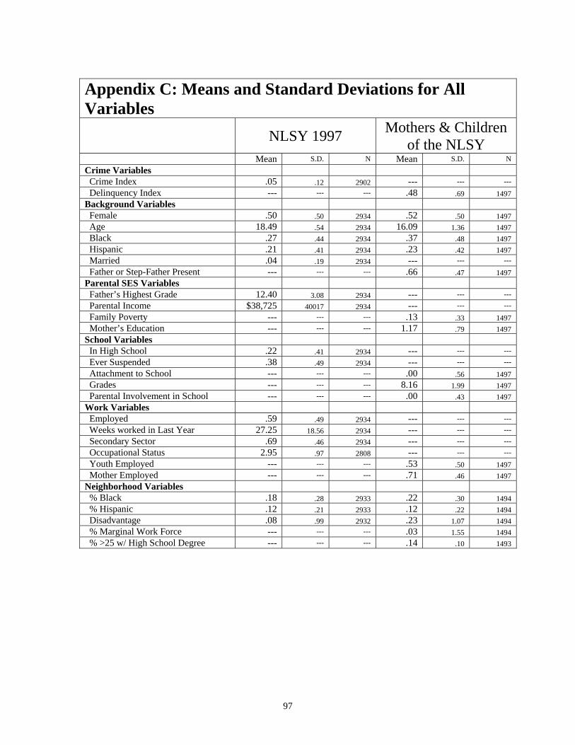
97

Appendix C: Means and Standard Deviations for All Variables

NLSY 1997 Mothers & Children of the NLSY

Mean S.D. N Mean S.D. N Crime Variables Crime Index .05 .12 2902 --- --- --- Delinquency Index --- --- --- .48 .69 1497 Background Variables Female .50 .50 2934 .52 .50 1497 Age 18.49 .54 2934 16.09 1.36 1497 Black .27 .44 2934 .37 .48 1497 Hispanic .21 .41 2934 .23 .42 1497 Married .04 .19 2934 --- --- --- Father or Step-Father Present --- --- --- .66 .47 1497 Parental SES Variables Father’s Highest Grade 12.40 3.08 2934 --- --- --- Parental Income $38,725 40017 2934 --- --- --- Family Poverty --- --- --- .13 .33 1497 Mother’s Education --- --- --- 1.17 .79 1497 School Variables In High School .22 .41 2934 --- --- --- Ever Suspended .38 .49 2934 --- --- --- Attachment to School --- --- --- .00 .56 1497 Grades --- --- --- 8.16 1.99 1497 Parental Involvement in School --- --- --- .00 .43 1497 Work Variables Employed .59 .49 2934 --- --- --- Weeks worked in Last Year 27.25 18.56 2934 --- --- --- Secondary Sector .69 .46 2934 --- --- --- Occupational Status 2.95 .97 2808 --- --- --- Youth Employed --- --- --- .53 .50 1497 Mother Employed --- --- --- .71 .46 1497 Neighborhood Variables % Black .18 .28 2933 .22 .30 1494 % Hispanic .12 .21 2933 .12 .22 1494 Disadvantage .08 .99 2932 .23 1.07 1494 % Marginal Work Force --- --- --- .03 1.55 1494 % >25 w/ High School Degree --- --- --- .14 .10 1493

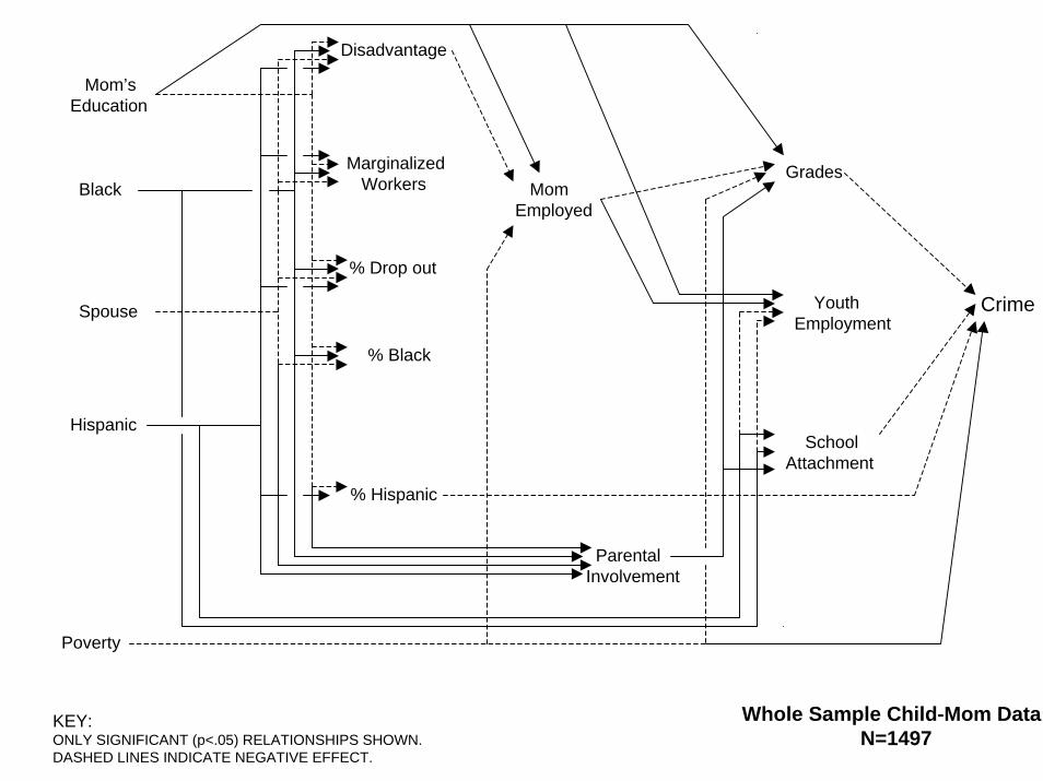
Mom’s Education

Hispanic

Poverty

Disadvantage

Marginalized Workers

% Hispanic

% Drop out

GradesMom

Employed

Parental Involvement

Youth Employment

Crime

Black

Spouse

% Black

School Attachment

Whole Sample Child-Mom Data N=1497

KEY:ONLY SIGNIFICANT (p<.05) RELATIONSHIPS SHOWN. DASHED LINES INDICATE NEGATIVE EFFECT.

Mom’s Education

Hispanic

Poverty

Disadvantage

Marginalized Workers

% Black

% Hispanic

% Drop out

GradesMom

Employed

Parental Involvement

Youth Employment

Crime

Black

Spouse

School Attachment

In SMSA Child-Mom Data N=1167

KEY:ONLY SIGNIFICANT (p<.05) RELATIONSHIPS SHOWN. DASHED LINES INDICATE NEGATIVE EFFECT.

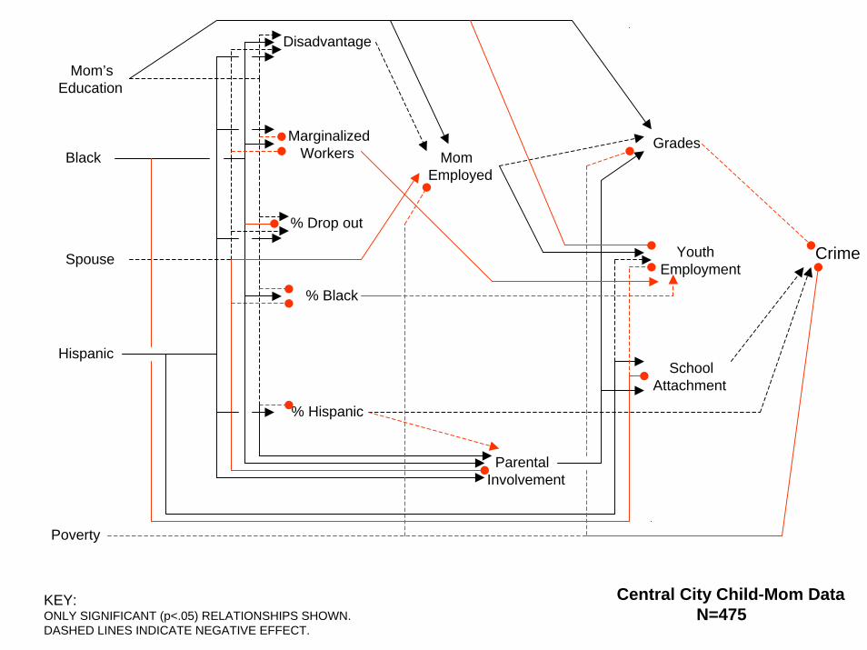
Mom’s Education

Hispanic

Poverty

Disadvantage

Marginalized Workers

% Black

% Hispanic

% Drop out

GradesMom

Employed

Parental Involvement

Youth Employment

Crime

Black

Spouse

School Attachment

Central City Child-Mom Data N=475

KEY:ONLY SIGNIFICANT (p<.05) RELATIONSHIPS SHOWN. DASHED LINES INDICATE NEGATIVE EFFECT.

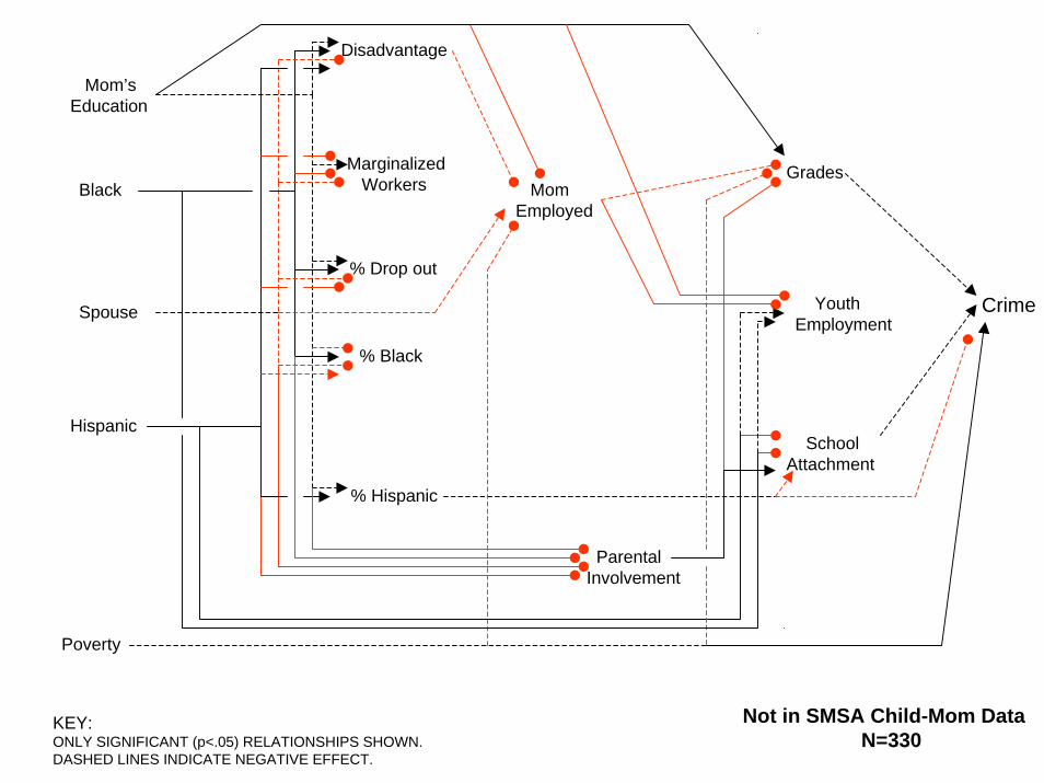
Mom’s Education

Hispanic

Poverty

Disadvantage

Marginalized Workers

% Black

% Hispanic

% Drop out

GradesMom

Employed

School Attachment

Parental Involvement

Youth Employment

Crime

Black

Spouse

Not in SMSA Child-Mom Data N=330

KEY:ONLY SIGNIFICANT (p<.05) RELATIONSHIPS SHOWN. DASHED LINES INDICATE NEGATIVE EFFECT.