Labor Cost and Technology Adoption: Real Options Approach for the Case of Sugarcane Mechanization in Florida

Nobuyuki Iwai International Agricultural Trade & Policy Center

Food and Resource Economics Department PO Box 110240, University of Florida

Gainesville, FL 32611 niwai@ufl.edu

Robert D. Emerson International Agricultural Trade & Policy Center

Food and Resource Economics Department PO Box 110240, University of Florida

Gainesville, FL 32611 remerson@ufl.edu

Lurleen M. Walters International Agricultural Trade & Policy Center

Food and Resource Economics Department P.O. Box 110240, University of Florida

Gainesville, FL 32611 lwalters@ufl.edu

Abstract Specialty crop farmers have expressed concern about labor shortages and cost increases which may arise with immigration reform. The large-scale mechanization of the Florida sugarcane harvest during the 1970s/80s serves as an historical example of how technologies evolved due to changes in local labor market conditions.

Selected Paper prepared for presentation at the Southern Agricultural Economics Association Annual Meeting, Dallas, Texas, February 2-6, 2008.

Copyright 2008 by Nobuyuki Iwai, Robert D. Emerson, and Lurleen M. Walters. All rights reserved. Readers may make verbatim copies of this document for non-commercial purposes by any means, provided that this copyright notice appears on all such copies.

1

Labor Cost and Technology Adoption: Real Options Approach for the Case of Sugarcane Mechanization in Florida

Introduction

The prospect of immigration reform has renewed farmers’ concerns of serious labor shortages

and cost increases, given that a large percentage of the workforce is unauthorized for U.S.

employment (Preston 2007, Wall Street Journal 2007). Clearly, this is more of a concern for

specialty crop agriculture that is highly labor intensive. In addition to the large labor

requirements, labor use is often concentrated in a very short period, particularly at harvest time

(Emerson 2007). This concern about labor-cost-increase seems quite legitimate if, as implied by

the recent immigration reform proposals, only legal workers would be available for employers.

This is because existing literature suggests a significant wage gap between legal and illegal

workers (Taylor 1992; Ise and Perloff 1995; Iwai et al. 2006).

There are several ways in which agricultural employers could deal with increased labor

cost, but the most likely ones in the mid- to long-term would be the adoption of a technology

with less labor use, and termination of current crop production if an alternative technology is not

available (Emerson 2007). Mechanical harvesting is a typical example of the former option,

whereas the latter option may involve changes to the cropping mix such that less labor is

required. The large-scale mechanization of the Florida sugarcane harvest during the 1970s/80s

serves as an historical example of how technologies evolved due to changes in local labor market

conditions. Anecdotally, it is said that increases in labor cost forced sugarcane farmers to switch

to mechanical harvesting.1

Several studies of Florida sugarcane production have compared the cost and returns from

mechanically harvested operations with those of hand cutting operations for the relevant period

(Zepp and Clayton 1975, Zepp 1975). Based on data for the 1972-73 season, Zepp and Clayton

2

1 Zepp (1975) reports that the average hourly wage of workers hired for sugarcane production and harvesting in Florida was 1.348 dollars for 1964-65 season, but it went up to 2.465 dollars for 1972-73 season for which period 15 percent of the Florida sugarcane crop was harvested mechanically.

(1975) found that the direct expenses (such as those for machinery and labor) were less per ton of

cane when mechanical harvesting was used. However, these lower costs were more than offset

by reduced revenue due to large field losses and higher trash content with mechanical harvesting,

resulting in $40.70 lower net returns per acre in comparison to hand-cut cane. If projected

1974-75 machinery operating rates had been used, the net returns per acre would have been

about equal for the two harvesting methods, and the additional 10% labor cost increase would

have been sufficient to overturn the net returns advantage (Zepp 1975).

Another important study on cost structure of Florida sugarcane farmers is Walker (1972)

which estimates the production cost for all activities including harvesting for the model farmer,

but does not distinguish the mode of harvesting.2 All of these previous studies calculated and

compared the cost and returns from two technologies for a single individual season. By contrast,

our analysis develops the dynamic decision-making process of farmers. There are two main

approaches for that purpose: net present value (NPV) approach and real options approach

(ROA).

The NPV approach simply assumes that the producer invests if the NPV of the

investment is greater than zero. In the case of Florida sugarcane, the farmer will switch to

mechanical harvesting if the discounted future cash flow less the investment cost for mechanical

operation is higher than the discounted future cash flow from the current operation. The ROA,

which applies financial option theory for investment in real assets, assumes that the producer has

the option to invest or wait, called “investment flexibility”. However, once the producer makes

an irreversible investment, he exercises, or “kills” the option to invest and gives up the value of

keeping the investment option alive. Hence the producer does not invest until the NPV of

mechanical harvesting operation less the option value is greater than the NPV of hand cut

3

2 Zepp and Clayton (1975) and Zepp (1975) use the cost estimate other than harvesting from Walker (1972), and use it as “production (growing) cost”.

operation (Dixit and Pindyck 1994, Trigeorgis 1996). The consideration for flexibility and

irreversibility of investment in the real options approach often yields a much higher trigger value

of the return (or cash flow) from mechanized harvesting operation than that calculated from NPV

approach, delaying the investment decision until higher profit is more likely.3 Although we do

not have an a priori preference over either method, the ROA is supposed to yield more

reasonable results.4 Since sugarcane farmers obviously have the ability to postpone their decision

on investment, and, in general, investment in agriculture is at least partially irreversible

(Napasintuwong and Emerson 2004),5 the consideration for these aspects of investment is

important.

In the current study, we use these two methods to analyze the decision of the average

sugarcane farmer in Florida as to mechanization of harvesting at the time of the 1972-3 season.

We also compute the adoption thresholds for the labor cost that triggered investment in

mechanical harvesting for sugarcane in Florida. These methods also can incorporate another

source of uncertainty which is said to be the other important factor causing the shift to

mechanized harvesting: yield and price of sugarcane, and costs other than labor. We use these

variables in our model.

There are several ways this study contributes to the literature of agricultural economics.

First, although there are studies which use the real options approach for the analysis of

technology adoption in agriculture (Seo et al. 2006, Engel and Hyde 2003, Carey and Zilberman

2002), none focuses on the impact of labor market conditions on technology adoption. Given the

3 Real options approach can handle partially reversible investment decision. In our case this means that sugarcane farmer can turn back to hand cutting harvesting with some cost. 4 Some studies on technology adoption in agriculture support the validity of the ROA over the NPV approach (Seo et al. 2006, Engel and Hyde 2003, Carey and Zilberman 2002). These studies generally show that farmers would not invest in an alternative technology until the present value of investment exceeds the investment cost by a potentially large hurdle rate. 5 Napasintuwong and Emerson (2004) show that it is harder to substitute labor for capital when capital becomes expensive than it is to substitute capital for labor when labor becomes expensive.

4

current heated debate over proposed immigration reform, this is a crucial issue which should be

analyzed. The current study analyzes the decision of the average sugarcane farmer in Florida as

to mechanization of harvesting at the time of 1972-3 season, and computes the threshold value

for labor costs which triggered the mechanical harvesting. Second, the current study builds the

foundation for forecasting the possible effect of labor cost increases on the adoption of less

labor-intensive operations. The study of the Florida sugarcane harvesting case helps us to

forecast the timing and scale of adoption of mechanization for certain crops for which

mechanized operation technology has already been developed, but not widely adopted (such as

citrus).

Methodology

We use the NPV and real options approach (ROA) to analyze the mechanization decision of

Florida sugarcane farmers and compute the adoption thresholds for labor cost that triggered

investment in mechanical harvesting for sugarcane in Florida. The NPV approach compares the

present value of forecasted free cash flow (FCF) less the investment cost for the mechanical

operation, with the present value of forecasted free cash flow for the current operation. The most

important part of the NPV approach is to forecast the future free cash flows for each operation.

We model and estimate the stochastic process for yield, price, labor cost and other costs, and run

the Monte Carlo simulation to have the FCF forecast.

In the real options approach, the value of the investment opportunity (the value of the

option to invest) as well as the present value of discounted FCF from each technology has to be

computed. In general, the value of the investment opportunity does not have a closed form

solution, except for the case with a single source of uncertainty that follows a basic stochastic

process (such as the geometric Brownian motion). Since there are four sources of uncertainty in

the current study we use a numerical method called consolidation approach which we explain in

5

detail in the following sections.

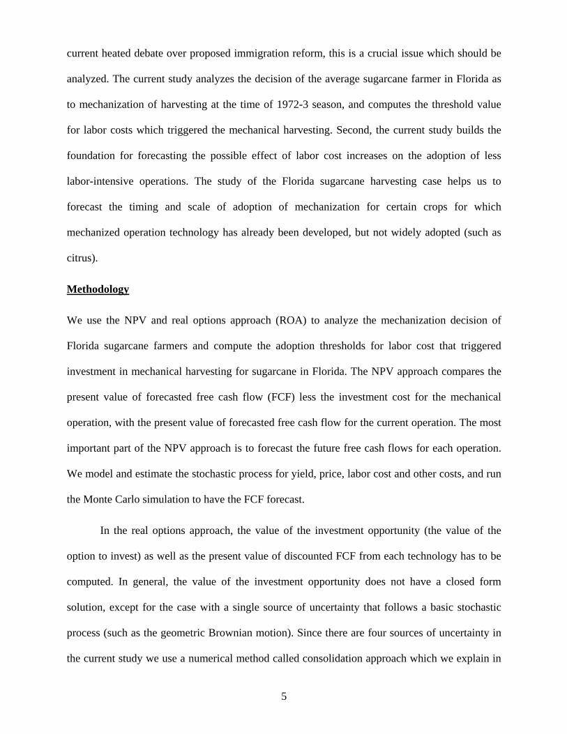
Data

The most important source of data is cost for growing sugarcane from Walker (1972) and

revenue and cost for harvesting sugarcane from Zepp and Clayton (1975). The second column of

Table 1 shows activity-base cost for growing sugarcane for the model farm with 640 acres in

total and 408 acres harvested in south Florida 1971-2 season, and the third column shows the

forecasted value for each item provided by Walker (1972).

Table 1. Activity-base cost for growing sugarcane for the model farm with 640 acres in total and 408 acres harvested ($ per 408 acres harvested) Season 1971-2 1972-3 Land preparation 6,131.35 6,437.92Planting 13,816.94 14,507.79Cultivate plant cane 4,970.96 5,219.51Cultivate stubble cane 8,480.96 8,905.01Overhead expense 14,351.94 15,069.54Overhead taxes 7,648.00 8,030.40Cost of land 53,760.00 56,448.00Total 109,160.15 114,618.16

Source: Walker (1972).

We convert the above table to cost-item base. The result is shown as Table 2.

Table 2. Cost for growing sugarcane for a model farm with 640 acres in total and 408 acres harvested ($ per 408 acres harvested) Season 1971-2 1972-3 Labor 11,352.66 11,920.29Depreciation 7,044.24 7,396.45Interest 4,514.51 4,740.24Other costs 86,248.74 90,561.18Total 109,160.15 114,618.16

Source: Authors calculated from Walker (1972).

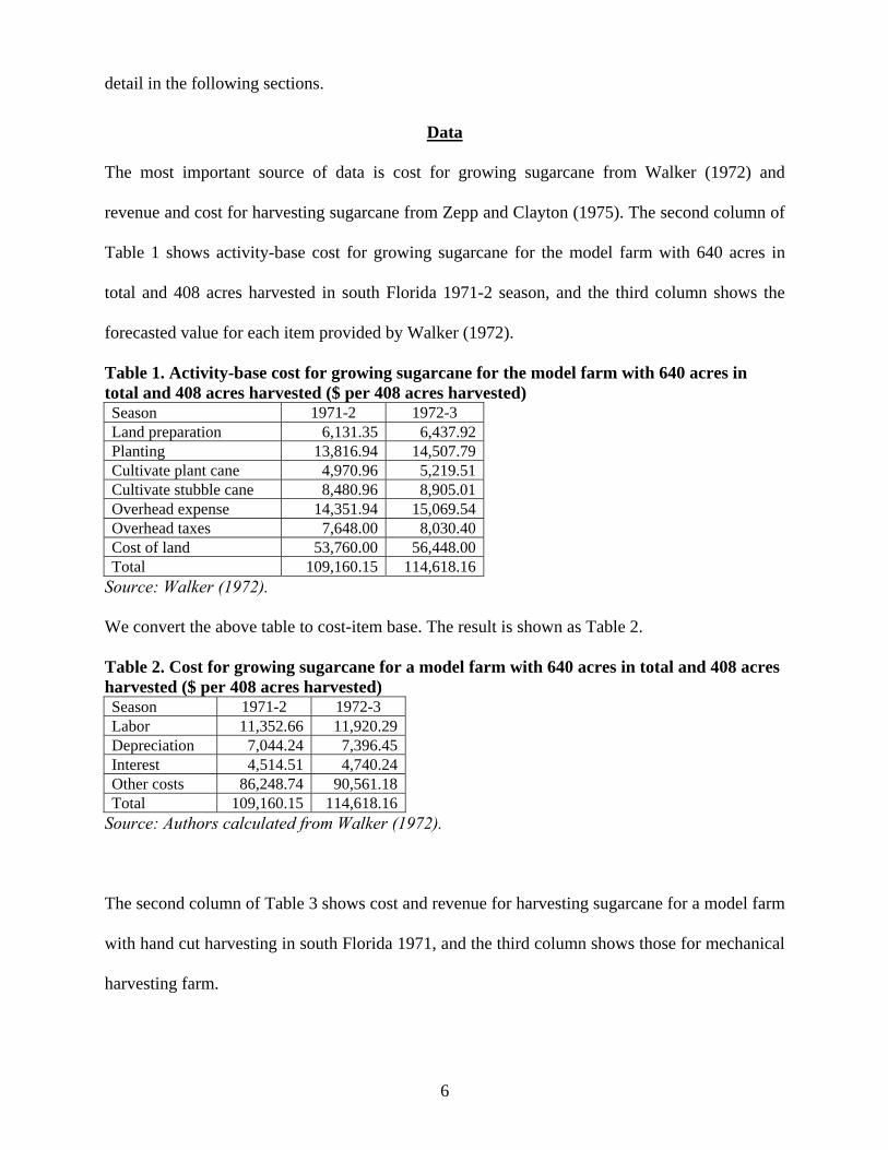
The second column of Table 3 shows cost and revenue for harvesting sugarcane for a model farm

with hand cut harvesting in south Florida 1971, and the third column shows those for mechanical

harvesting farm.

6

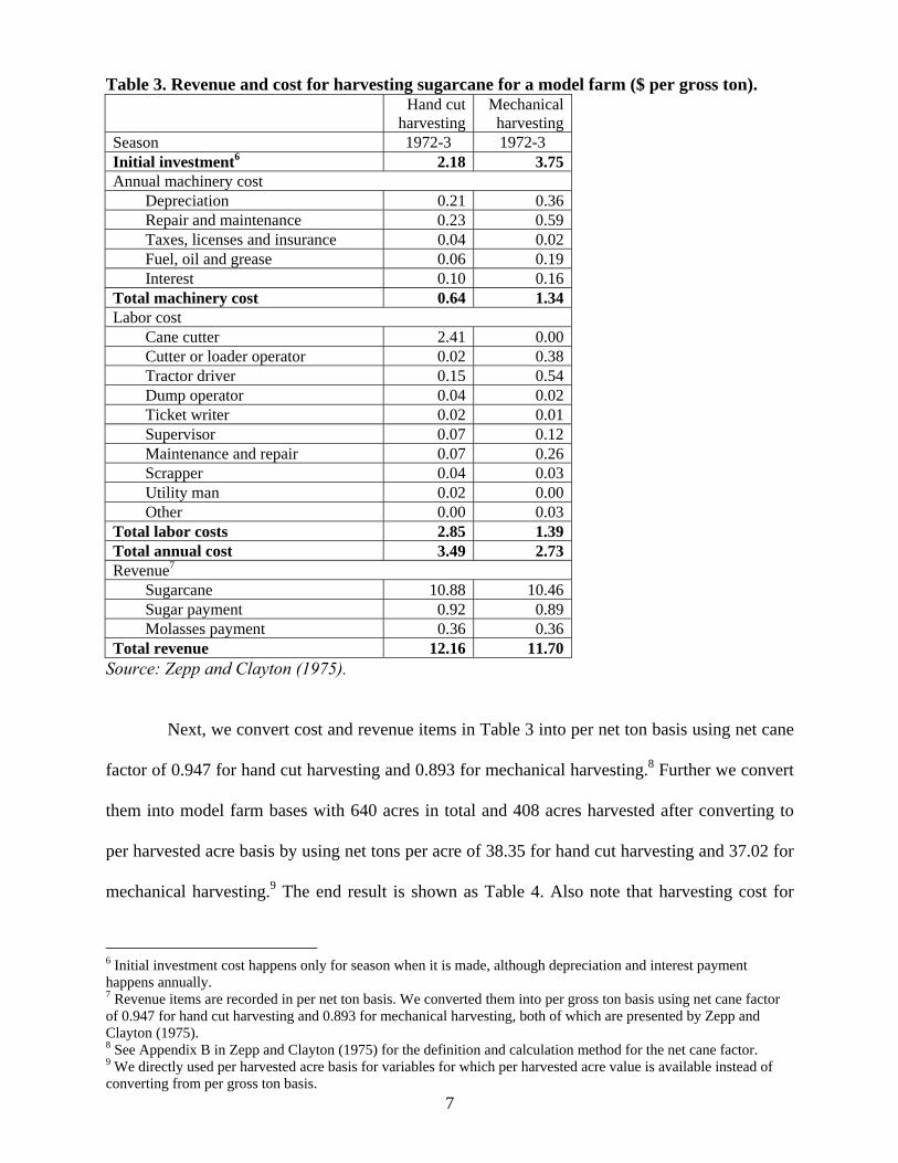
Table 3. Revenue and cost for harvesting sugarcane for a model farm ($ per gross ton).

Hand cut

harvestingMechanical harvesting

Season 1972-3 1972-3 Initial investment6 2.18 3.75Annual machinery cost Depreciation 0.21 0.36 Repair and maintenance 0.23 0.59 Taxes, licenses and insurance 0.04 0.02 Fuel, oil and grease 0.06 0.19 Interest 0.10 0.16Total machinery cost 0.64 1.34Labor cost Cane cutter 2.41 0.00 Cutter or loader operator 0.02 0.38 Tractor driver 0.15 0.54 Dump operator 0.04 0.02 Ticket writer 0.02 0.01 Supervisor 0.07 0.12 Maintenance and repair 0.07 0.26 Scrapper 0.04 0.03 Utility man 0.02 0.00 Other 0.00 0.03Total labor costs 2.85 1.39Total annual cost 3.49 2.73Revenue7

Sugarcane 10.88 10.46 Sugar payment 0.92 0.89 Molasses payment 0.36 0.36Total revenue 12.16 11.70

Source: Zepp and Clayton (1975).

Next, we convert cost and revenue items in Table 3 into per net ton basis using net cane

factor of 0.947 for hand cut harvesting and 0.893 for mechanical harvesting.8 Further we convert

them into model farm bases with 640 acres in total and 408 acres harvested after converting to

per harvested acre basis by using net tons per acre of 38.35 for hand cut harvesting and 37.02 for

mechanical harvesting.9 The end result is shown as Table 4. Also note that harvesting cost for

6 Initial investment cost happens only for season when it is made, although depreciation and interest payment happens annually. 7 Revenue items are recorded in per net ton basis. We converted them into per gross ton basis using net cane factor of 0.947 for hand cut harvesting and 0.893 for mechanical harvesting, both of which are presented by Zepp and Clayton (1975). 8 See Appendix B in Zepp and Clayton (1975) for the definition and calculation method for the net cane factor.

7

9 We directly used per harvested acre basis for variables for which per harvested acre value is available instead of converting from per gross ton basis.

73-4 and 74-5 season are revised according to forecast from Zepp and Clayton (1975). They

forecast no change in all other items.

Table 4. Revenue and cost for growing and harvesting sugarcane for a model farm ($ per 408 acres harvested)

Hand cut harvesting

Mechanical harvesting

Mechanical harvesting

Mechanical harvesting

Season 72-5 72-3 73-4 74-5 Revenue Sugarcane 190,597.20 176,896.56 176,896.56 176,896.56 Sugar payment 16,169.04 15,026.64 15,026.64 15,026.64 Molasses payment 6,238.32 6,022.08 6,022.08 6,022.08 Total revenue 213,004.56 197,945.28 197,945.28 197,945.28 Cost Growing Labor 11,920.29 11,920.29 11,920.29 11,920.29 Depreciation 7,396.45 7,396.45 7,396.45 7,396.45 Interest expenses 4,740.24 4,740.24 4,740.24 4,740.24 Other costs 90,561.18 90,561.18 90,561.18 90,561.18 Total 114,618.16 114,618.16 114,618.16 114,618.16 Harvesting Labor 47,095.44 23,863.92 17,767.27 11,670.63 Depreciationa 3,459.15 6,172.75 6,172.75 6,172.75 Interest expenses 1,588.31 2,788.27 2,788.27 2,788.27 Other costs 5,434.06 13,695.23 12,107.01 10,518.79 Total 57,576.96 46,520.16 38,835.29 31,150.43 Total cost 172,195.12 161,138.32 153,453.45 145,768.58 Return 40,809.44 36,806.96 44,491.83 52,176.70

Source: Authors calculated from Zepp and Clayton (1975). a Both Zepp and Clayton (1975) and Walker (1972) assume that depreciation and interest expenses are based on the initial investment value. Here we assume that the farmer is currently using hand cut harvesting so that depreciation and interest expenses are fixed on the current level for the hand cut harvesting, and they are fixed on the level of 72-3 season for the mechanical harvesting since we analyze the decision in that season.

Other data we need to use for the current study are those to forecast the revenue and cost

after 1974-5 season since Zepp and Clayton (1975) have explicit forecasts up to only the 1974-5

season. We use market data for time series of sugarcane yield, price, labor cost and other costs.

We use the sugarcane yield and price data from the Florida Field Crops Summary (Florida

Agricultural Statistics). The labor cost data are from unpublished U.S. Department of Labor

administrative records pertaining specifically to labor employed in Florida sugarcane; the other

cost data is similarly from unpublished U.S. Department of Agriculture administrative records.

We use the time series of sugarcane yield and price as long as possible but still in the relevant

8

period: 1960-95. On the other hand, the time series of labor cost and other costs have many

missing periods so that we use the following more restricted period to estimate the stochastic

process: 1960-81.

Traditional NPV approach

In this section we analyze the mechanization decision by Florida sugarcane farmers using the

NPV approach, which is the single, most widely used tool for large investments made by U.S.

corporations (Copeland and Antikarov 2003). Although the implementation of the approach

involves many steps, the basic concept of it is rather simple: the farmer would invest in

mechanization if the discounted future free cash flow (FCF) forecasted for the

mechanical-harvesting-operation less the investment cost is greater than that from the

hand-cut-operation. Therefore, the first step of the approach is to estimate future FCF for each

operational mode using estimates from Zepp and Clayton (1975) and Walker (1972). Then, we

model and estimate the stochastic process of sugarcane yield, price, labor cost and other costs

and run the Monte Carlo simulation to forecast FCF for the years after 1975. The forecasted FCF

from each operation (the entity value) should be discounted at the opportunity cost of capital that

is consistent with riskiness of these cash flows. We compute this discount rate which is called

“Weighted Average Cost of Capital (WACC)”. The straightforward calculation of discounted

free cash flow for each operational mode follows the above steps.10

Estimating FCF

The value of operation equals the discounted value of future FCF which is equal to the after-tax

operating earnings of the farm, plus non-cash charges, less investments in operating working

capital, property, and other assets (Copeland et al. 1994). This is the correct cash flow for this

valuation model since it reflects the cash flow that is generated by a farm’s operation and

available to all capital providers, both debt and equity.

9

10 This method called entity DCF model is mathematically equivalent to equity DCF model in which free cash flows to equity is discounted at the cost of equity.

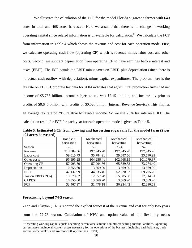
We illustrate the calculation of the FCF for the model Florida sugarcane farmer with 640

acres in total and 408 acres harvested. Here we assume that there is no change in working

operating capital since related information is unavailable for calculation.11 We calculate the FCF

from information in Table 4 which shows the revenue and cost for each operation mode. First,

we calculate operating cash flow (operating CF) which is revenue minus labor cost and other

costs. Second, we subtract depreciation from operating CF to have earnings before interest and

taxes (EBIT). The FCF equals the EBIT minus taxes on EBIT, plus depreciation (since there is

no actual cash outflow with depreciation), minus capital expenditures. The problem here is the

tax rate on EBIT. Corporate tax data for 2004 indicates that agricultural production firms had net

income of $5.756 billion, income subject to tax was $2.151 billion, and income tax prior to

credits of $0.646 billion, with credits of $0.020 billion (Internal Revenue Service). This implies

an average tax rate of 29% relative to taxable income. So we use 29% tax rate on EBIT. The

calculation result for FCF for each year for each operation mode is given as Table 5.

Table 5. Estimated FCF from growing and harvesting sugarcane for the model farm ($ per 404 acres harvested)

Hand cut

harvesting Mechanical harvesting

Mechanical harvesting

Mechanical harvesting

Season 72-5 72-3 73-4 74-5 Revenue 213,004.56 197,945.28 197,945.28 197,945.28Labor cost 59,015.73 35,784.21 29,687.56 23,590.92Other costs 95,995.25 104,256.41 102,668.19 101,079.97Operating CF 57,993.59 57,904.66 65,589.53 73,274.40Depreciation 10,855.60 13,569.20 13,569.20 13,569.20EBIT 47,137.99 44,335.46 52,020.33 59,705.20Tax on EBIT (29%) 13,670.02 12,857.28 15,085.90 17,314.51CAPEX 10,855.60 13,569.20 13,569.20 13,569.20F F C 33,467.97 31,478.18 36,934.43 42,390.69

Forecasting beyond 74-5 season

Zepp and Clayton (1975) reported the explicit forecast of the revenue and cost for only two years

from the 72-73 season. Calculation of NPV and option value of the flexibility needs

10

11 Operating working capital equals operating current assets minus noninterest bearing current liabilities. Operating current assets include all current assets necessary for the operations of the business, including cash balances, trade accounts receivables, and inventories (Copeland et al. 1994).

longer-period forecasts beyond two years which reflect the future cash flow process the farmers

were facing at the decision time. A common approach often used in simulation studies is the

Monte Carlo simulation in which all stochastic series are generated for future periods using the

estimated parameters and distributions of these series (Kobayashi 2003, Copeland and Antikarov

2003). Therefore, modeling and estimating the stochastic process for time series is a crucial step

for the Monte Carlo simulation. Here we follow the approach suggested by Brockwell and Davis

(1991, 2002). The first step suggested is creating a stationary process by transforming the time

series of interest.12

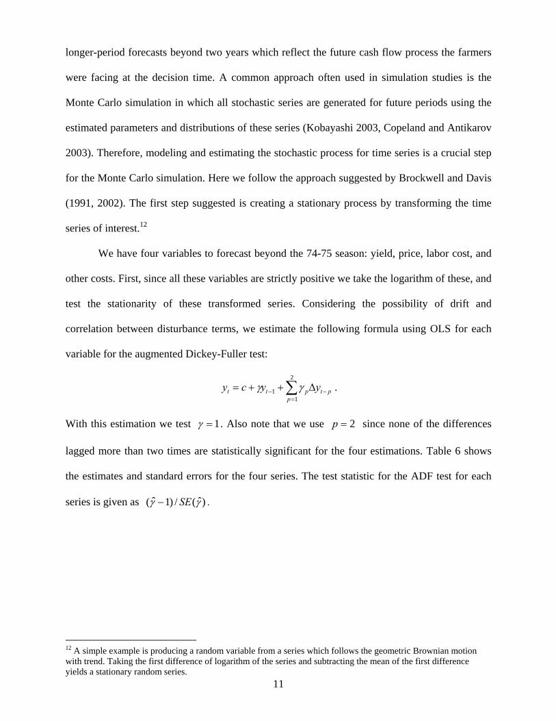
We have four variables to forecast beyond the 74-75 season: yield, price, labor cost, and

other costs. First, since all these variables are strictly positive we take the logarithm of these, and

test the stationarity of these transformed series. Considering the possibility of drift and

correlation between disturbance terms, we estimate the following formula using OLS for each

variable for the augmented Dickey-Fuller test:

∑=

−− ∆++=2

11

pptptt yycy γγ .

With this estimation we test 1=γ . Also note that we use 2=p since none of the differences

lagged more than two times are statistically significant for the four estimations. Table 6 shows

the estimates and standard errors for the four series. The test statistic for the ADF test for each

series is given as )ˆ(/)1ˆ( γγ SE− .

11

12 A simple example is producing a random variable from a series which follows the geometric Brownian motion with trend. Taking the first difference of logarithm of the series and subtracting the mean of the first difference yields a stationary random series.

Table 6. Estimated coefficients, standard errors, and ADF test statistics Yield Price Labor cost Other costs

c 3.49 (1.15)

0.35 (0.23)

-0.10 (0.34)

-1.18 (0.98)

γ -0.0045 (0.33)

0.90 (0.08)

1.05 (0.09)

1.15 (0.11)

1γ -0.0051 (0.25)

0.12 (0.16)

-0.28 (0.25)

-0.55 (0.27)

2γ -0.18 (0.18)

-0.44 (0.16)

-0.43 (0.24)

-0.47 (0.28)

Observations 33 33 19 19 ADF test -3.03 -1.32 0.56 1.34

Since the critical value with 5 % level of significance is approximately -3.00 for 19

observations, and -2.97 for 33 observations, we can barely reject the null hypothesis of a unit

root for the log of yield, but cannot reject the null hypothesis for all others. Then we take the first

difference of each series and repeat the same test procedure for the transformed data.13 The

results are shown in Table 7. The test results show that the first difference is enough to produce

the stationary process from each series. We further subtract the sample mean of the transformed

series from the transformed series.14

Table 7. Estimated coefficients, standard errors, and ADF test statistics after taking the first difference Yield Price Labor cost Other costs

c 0.00 (0.01)

0.053 (0.041)

0.09 (0.04)

0.13 (0.05)

γ -1.18 (0.25)

-0.40 (0.22)

-0.62 (0.35)

-0.65 (0.39)

1γ 0.54 (0.15)

0.48 (0.16)

0.39 (0.23)

0.27 (0.24)

No. of observation 33 33 19 19ADF test -8.63 -6.37 -4.66 -4.24

The next step is to model the generated residuals obtained by differencing the series and

subtracting the sample mean of the difference. If there is no dependence among these residuals,

we can regard them as observations of independent random variables. However, if there is

13 We use p=1 since the only statistically significant lagged difference is the first one.

12

14 If the series follows the geometric Brownian motion with trend, these steps are enough to produce an iid random series with zero mean.

significant dependence among the residuals, we need to look for a more complex stationary time

series model to account for the dependence. This will be to our advantage since dependence

means that past observations of the residual sequence can assist in predicting future values. Here

we implement some tests for the hypothesis that the residuals generated above are observations

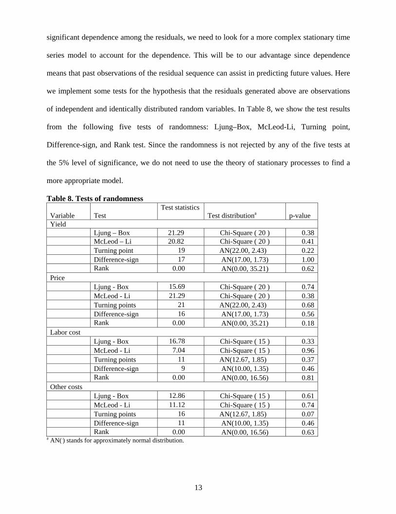
of independent and identically distributed random variables. In Table 8, we show the test results

from the following five tests of randomness: Ljung–Box, McLeod-Li, Turning point,

Difference-sign, and Rank test. Since the randomness is not rejected by any of the five tests at

the 5% level of significance, we do not need to use the theory of stationary processes to find a

more appropriate model.

Table 8. Tests of randomness

Variable

Test Test statistics

Test distributiona p-value Yield Ljung – Box 21.29 Chi-Square ( 20 ) 0.38 McLeod – Li 20.82 Chi-Square ( 20 ) 0.41 Turning point 19 AN(22.00, 2.43) 0.22 Difference-sign 17 AN(17.00, 1.73) 1.00 Rank 0.00 AN(0.00, 35.21) 0.62 Price Ljung - Box 15.69 Chi-Square ( 20 ) 0.74 McLeod - Li 21.29 Chi-Square ( 20 ) 0.38 Turning points 21 AN(22.00, 2.43) 0.68 Difference-sign 16 AN(17.00, 1.73) 0.56 Rank 0.00 AN(0.00, 35.21) 0.18 Labor cost Ljung - Box 16.78 Chi-Square ( 15 ) 0.33 McLeod - Li 7.04 Chi-Square ( 15 ) 0.96 Turning points 11 AN(12.67, 1.85) 0.37 Difference-sign 9 AN(10.00, 1.35) 0.46 Rank 0.00 AN(0.00, 16.56) 0.81 Other costs Ljung - Box 12.86 Chi-Square ( 15 ) 0.61 McLeod - Li 11.12 Chi-Square ( 15 ) 0.74 Turning points 16 AN(12.67, 1.85) 0.07 Difference-sign 11 AN(10.00, 1.35) 0.46 Rank 0.00 AN(0.00, 16.56) 0.63

a AN(.) stands for approximately normal distribution.

13

However, further consideration is needed about the potential interdependence between

residuals. That is, multivariate time series {Xt} may have not only serial dependence within each

component series but also interdependence between the different component series {Xti} and

{Xtj}, i ≠ j. In the current case, the interdependence between cost series and between yield and

price is tested because of the mismatch in the number of observations. The second-order

properties of the multivariate time series {Xt} are specified by the mean vector µt = and

covariance matrix

⎥⎦

⎤⎢⎣

⎡

2

1

t

t

µµ

Γ(t+h,t) , ⎥⎦

⎤⎢⎣

⎡++++

=),(),(),(),(

2221

1211

thtthtthttht

γγγγ

where ),cov() ,( ,, jhtihtij XXtht ++=+γ , but )() ,( htht ijij γγ =+ for stationary series so that

Γ(t+h,t) = Γ(h) and µt = µ.

Since the random white noise assumption is not rejected by the test of randomness for all

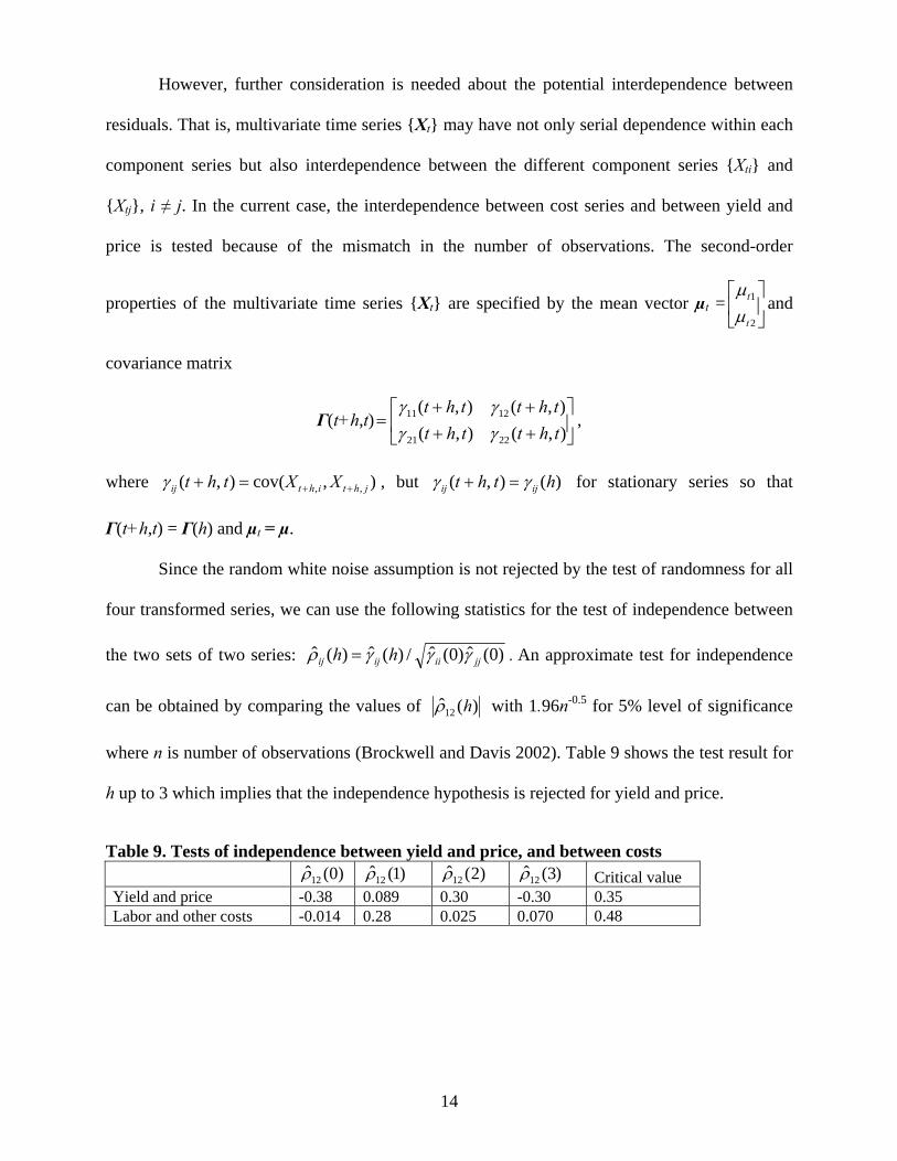
four transformed series, we can use the following statistics for the test of independence between

the two sets of two series: )0(ˆ)0(ˆ/)(ˆ)(ˆ jjiiijij hh γγγρ = . An approximate test for independence

can be obtained by comparing the values of )(ˆ12 hρ with 1.96n-0.5 for 5% level of significance

where n is number of observations (Brockwell and Davis 2002). Table 9 shows the test result for

h up to 3 which implies that the independence hypothesis is rejected for yield and price.

Table 9. Tests of independence between yield and price, and between costs )0(ˆ12ρ )1(ˆ12ρ )2(ˆ12ρ )3(ˆ12ρ Critical value Yield and price -0.38 0.089 0.30 -0.30 0.35 Labor and other costs -0.014 0.28 0.025 0.070 0.48

14

Since the test of independence is rejected for the former, we need to model for interdependence

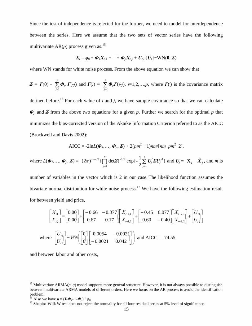
between the series. Here we assume that the two sets of vector series have the following

multivariate AR(p) process given as.15

Xt = φ0 + Φ1Xt-1 + … + ΦpXt-p + Ut, {Ut}~WN(0, Σ)

where WN stands for white noise process. From the above equation we can show that

Σ = Γ(0) ΦΣ=

p

j 1p Γ(-j) and Γ(i) = ΦΣ

=

p

j 1pΓ(i-j), i=1,2,…,p, where Γ(.) is the covariance matrix

defined before.16 For each value of i and j, we have sample covariance so that we can calculate

Φp and Σ from the above two equations for a given p. Further we search for the optimal p that

minimizes the bias-corrected version of the Akaike Information Criterion referred to as the AICC

(Brockwell and Davis 2002):

AICC = 2lnL(Φ1,…, Φp, Σ) + 2(pm2 + 1)nm/[nm pm2 2],

where L(Φ1,…, Φp, Σ) = detΠ=

−n

j

nm

1

2/ {)2( π Σ}-1/2 exp{- Σ=

n

j 121 Uj

’ΣUj-1} and Uj = , and m is

number of variables in the vector which is 2 in our case.

jj X̂−X

The likelihood function assumes the

bivariate normal distribution for white noise process.17 We have the following estimation result

for between yield and price,

⎥⎦

⎤⎢⎣

⎡+⎥

⎦

⎤⎢⎣

⎡⎥⎦

⎤⎢⎣

⎡−

−+⎥

⎦

⎤⎢⎣

⎡⎥⎦

⎤⎢⎣

⎡ −−+⎥

⎦

⎤⎢⎣

⎡=⎥

⎦

⎤⎢⎣

⎡

−

−

−

−

2

1

2,2

1,2

2,1

1,1

2

1

40.060.0077.045.0

17.067.0077.066.0

00.000.0

t

t

t

t

t

t

t

t

UU

XX

XX

XX

where and AICC = -74.55, ⎟⎟⎠

⎞⎜⎜⎝

⎛⎥⎦

⎤⎢⎣

⎡−

−⎥⎦

⎤⎢⎣

⎡⎥⎦

⎤⎢⎣

⎡042.00021.00021.00054.0

,00

~2

1 WNUU

t

t

and between labor and other costs,

15 Multivariate ARMA(p, q) model supports more general structure. However, it is not always possible to distinguish between multivariate ARMA models of different orders. Here we focus on the AR process to avoid the identification problem. 16 Also we have µ = (I-Φ1-…-Φp)-1 φ0.

1517 Shapiro-Wilk W test does not reject the normality for all four residual series at 5% level of significance.

⎥⎦

⎤⎢⎣

⎡+⎥

⎦

⎤⎢⎣

⎡=⎥

⎦

⎤⎢⎣

⎡

2

1

2

1

00.000.0

t

t

t

t

UU

XX

where and AICC = -38.65. ⎟⎟⎠

⎞⎜⎜⎝

⎛⎥⎦

⎤⎢⎣

⎡−

−⎥⎦

⎤⎢⎣

⎡⎥⎦

⎤⎢⎣

⎡027.000052.000052.0020.0

,00

~2

1 WNUU

t

t

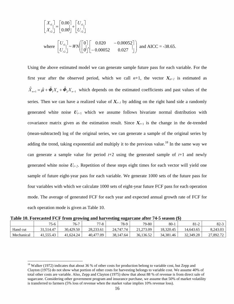
Using the above estimated model we can generate sample future pass for each variable. For the

first year after the observed period, which we call n+1, the vector Xn+1 is estimated as

which depends on the estimated coefficients and past values of the

series. Then we can have a realized value of X

1211ˆˆˆˆ

−+ ++= nnn XXX ΦΦµ

t+1 by adding on the right hand side a randomly

generated white noise Ut+1 which we assume follows bivariate normal distribution with

covariance matrix given as the estimation result. Since Xt+1 is the change in the de-trended

(mean-subtracted) log of the original series, we can generate a sample of the original series by

adding the trend, taking exponential and multiply it to the previous value.18 In the same way we

can generate a sample value for period t+2 using the generated sample of t+1 and newly

generated white noise Ut+2. Repetition of these steps eight times for each vector will yield one

sample of future eight-year pass for each variable. We generate 1000 sets of the future pass for

four variables with which we calculate 1000 sets of eight-year future FCF pass for each operation

mode. The average of generated FCF for each year and expected annual growth rate of FCF for

each operation mode is given as Table 10.

Table 10. Forecasted FCF from growing and harvesting sugarcane after 74-5 season ($) 75-6 76-7 77-8 78-9 79-80 80-1 81-2 82-3

Hand cut 31,514.47 30,429.50 28,233.61 24,747.74 21,273.09 18,320.45 14,643.65 8,243.03 Mechanical 41,555.43 41,624.24 40,477.09 38,147.64 36,136.52 34,381.46 32,349.28 27,892.72

16

18 Walker (1972) indicates that about 36 % of other costs for production belong to variable cost, but Zepp and Clayton (1975) do not show what portion of other costs for harvesting belongs to variable cost. We assume 40% of total other costs are variable. Also, Zepp and Clayton (1975) show that about 88 % of revenue is from direct sale of sugarcane. Considering other government program and insurance purchase, we assume that 50% of market volatility is transferred to farmers (5% loss of revenue when the market value implies 10% revenue loss).

From Tables 5 and 10 we calculate the expected growth rate of FCF for each mode: -12.06% for

hand cut harvesting, and -0.80% for mechanical harvesting operation.19

Weighted Average Cost of Capital

Now that we have estimated future free (entity) cash flows, the next step is to discount the FCF

by the appropriate discount rate. The discount rate we use is the weighted average cost of capital

(WACC) which is the time value of money used to convert the expected FCF into a present value

for all investors. Since entity cash flows are available for payment to both sources of capital, debt

and equity, the discount rate must comprise a weighted average of the marginal costs of both

sources of capital. In our application WACC is given by

SBSk

SBBTkWACC sb +

++

−= )1( ,

where kb is the pretax market expected yield to maturity on debt, T is the marginal tax rate for the

entity, which is 29% in our application, B is the market value of interest-bearing debt, and S is

the market value of equity, and ks is the market-determined opportunity cost of equity capital.

We take kb=8% directly from Zepp and Clayton (1975), and Walker (1972). We calculated the

debt to asset ratio for the fruitful rim for “other field crops” (includes sugar) averaged for the

years 1996-2005 (ARMS). The result is 0.12 so that we estimate B/(B+S)=0.12, and

S/(B+S)=0.88.20

Finally we estimate ks, the market-determined opportunity cost of equity capital. Here we

use the most widely used estimation method: capital asset pricing model (CAPM). The equation

for the cost of equity from the CAPM is given as

[ ] jfmfs rrErk β−+= )( ,

19 Expected growth rate calculation also uses estimated FCF for three seasons before 75-6 season (Table 5) which is based on the forecast provided by Zepp and Clayton (1975).

17

20 There are many other approaches to estimate the market value of equity. Especially, Copeland et al. (1994) suggests iteration method to deal with the circularity problem involved in estimating WACC and the market value of equity. However, we simply use the market average debt/asset ratio, since the necessary information is not available to implement the more involved method for our case study.

where rf is the risk-free rate of return, E(rm) is the expected rate of return on the overall market

portfolio, so that [E(rm)-rf ] is the market risk premium. jβ is the systematic risk of the equity

which is defined as COV(rj, rm)/VAR(rm) where rj is the rate of return from the equity to be

evaluated. We calculated geometric average of annual rate of return from Treasury bills for years

1960-95, and use it for the risk-free rate of return (rf =6.11%). We also calculated geometric

average of annual rate of return from stock using S&P 500 for the same period, and use it for the

overall market portfolio (E(rm )=10.67% and the risk premium=4.55%).21 We use the industry

beta for food and kindred products of 1.04 from Copeland et al. (1994), because this is the

industry with risk closest to the sugar industry. Using these figures we estimate for the WACC

approximately 10.23%.

NPV calculation

PV for year t is given as ( ) ( )( )gWACCWACC

FCFgWACC

FCFEPV tt

tt −++

++

= −+=

−∑ 19821982

1982

1 )1(1

)1(ττ

τ for t<1982.

( )( )gWACC

FCFgPV−

+= 1982

19821 . The latter is continuing value after the explicit forecast period estimated

using growing FCF perpetuity formula in which g is the expected growth rate in FCF in

perpetuity (-12.06% for hand cut harvesting, and -0.80% for mechanical harvesting operation). 22

NPV for year t simply adds FCF of that year to PV: ttt PVFCTNPV += ( It if the investment is

made in that year). We also calculate FCF as percentage of NPV for each year to be used for

ROA later. We show these figures in Table 11.

21 We calculated from dataset provided by Damodaran which is available at http://pages.stern.nyu.edu/~adamodar/pc/datasets/histretSP.xls.

18

22 Changing the assumption that the farmer continues to hold the operation after 82-3 season does not affect the value of PV, but the summation is taken over infinite future.

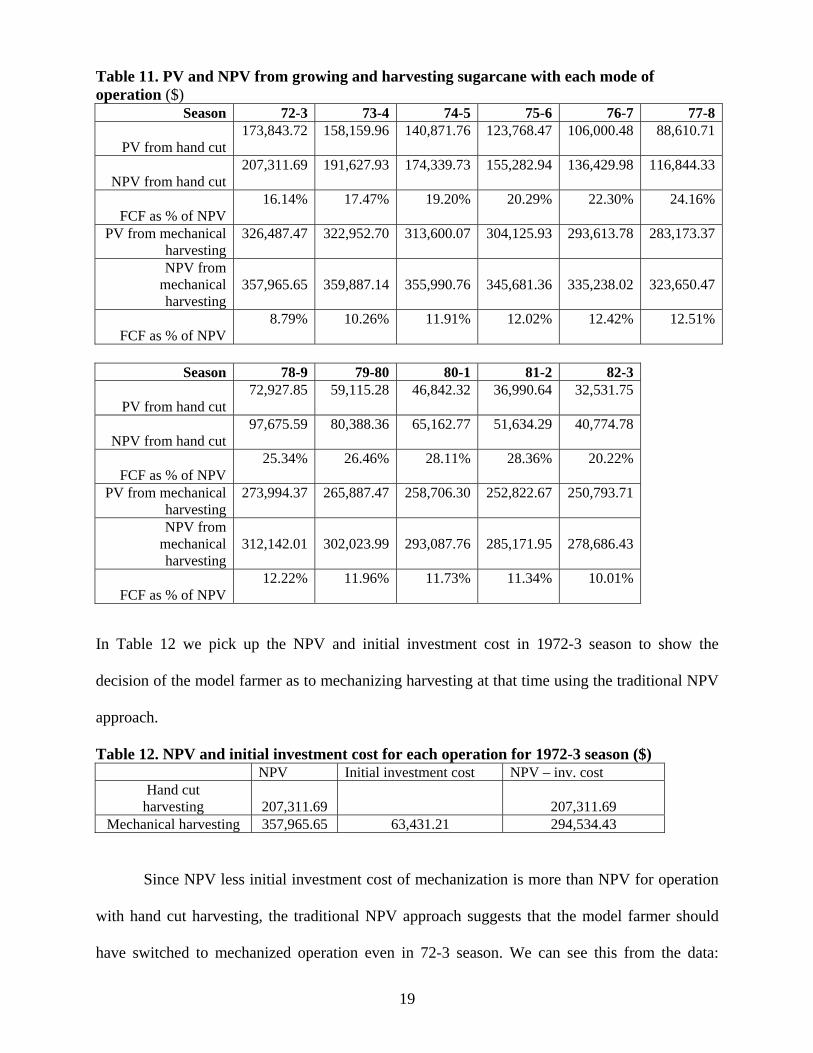
Table 11. PV and NPV from growing and harvesting sugarcane with each mode of operation ($)

Season 72-3 73-4 74-5 75-6 76-7 77-8

PV from hand cut 173,843.72

158,159.96 140,871.76 123,768.47 106,000.48

88,610.71

NPV from hand cut 207,311.69

191,627.93 174,339.73 155,282.94 136,429.98

116,844.33

FCF as % of NPV 16.14%

17.47% 19.20% 20.29% 22.30%

24.16%

PV from mechanical harvesting

326,487.47

322,952.70 313,600.07 304,125.93 293,613.78

283,173.37

NPV from mechanical harvesting

357,965.65

359,887.14 355,990.76 345,681.36 335,238.02

323,650.47

FCF as % of NPV 8.79%

10.26% 11.91% 12.02% 12.42%

12.51%

Season 78-9 79-80 80-1 81-2 82-3

PV from hand cut 72,927.85

59,115.28 46,842.32 36,990.64 32,531.75

NPV from hand cut 97,675.59

80,388.36 65,162.77 51,634.29 40,774.78

FCF as % of NPV 25.34%

26.46% 28.11% 28.36% 20.22%

PV from mechanical

harvesting 273,994.37

265,887.47 258,706.30 252,822.67 250,793.71

NPV from

mechanical harvesting

312,142.01

302,023.99 293,087.76 285,171.95 278,686.43

FCF as % of NPV 12.22%

11.96% 11.73% 11.34% 10.01%

In Table 12 we pick up the NPV and initial investment cost in 1972-3 season to show the

decision of the model farmer as to mechanizing harvesting at that time using the traditional NPV

approach.

Table 12. NPV and initial investment cost for each operation for 1972-3 season ($) NPV Initial investment cost NPV – inv. cost

Hand cut harvesting 207,311.69 207,311.69

Mechanical harvesting 357,965.65 63,431.21 294,534.43

Since NPV less initial investment cost of mechanization is more than NPV for operation

with hand cut harvesting, the traditional NPV approach suggests that the model farmer should

have switched to mechanized operation even in 72-3 season. We can see this from the data:

19

negative growth rate of FCF (12.05 %) and relatively high FCF/PV ratio (over 20%), that is,

growing and harvesting with hand cut operation generates relatively high FCF, but its expected

growth is negative in the future. In comparison the FCF of mechanized operation has relatively

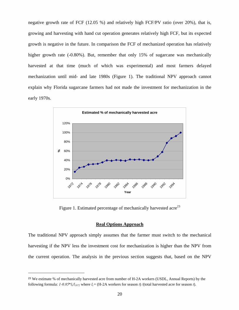
higher growth rate (-0.80%). But, remember that only 15% of sugarcane was mechanically

harvested at that time (much of which was experimental) and most farmers delayed

mechanization until mid- and late 1980s (Figure 1). The traditional NPV approach cannot

explain why Florida sugarcane farmers had not made the investment for mechanization in the

early 1970s.

Estimated % of mechanically harvested acre

0%

20%

40%

60%

80%

100%

120%

1972

1974

1976

1978

1980

1982

1984

1986

1988

1990

1992

1994

Year

%

Figure 1. Estimated percentage of mechanically harvested acre23

Real Options Approach

The traditional NPV approach simply assumes that the farmer must switch to the mechanical

harvesting if the NPV less the investment cost for mechanization is higher than the NPV from

the current operation. The analysis in the previous section suggests that, based on the NPV

23 We estimate % of mechanically harvested acre from number of H-2A workers (USDL, Annual Reports) by the following formula: 1-0.85*lt/l1972 where lt = (H-2A workers for season t) /(total harvested acre for season t).

20

approach, farmers should have already switched to mechanical harvesting in 1972-3 season.

However, only 15% of sugarcane was mechanically harvested at that time and most farmers

delayed mechanization until mid- and late 1980s; the NPV approach cannot offer an explanation

for this delay. The real options approach (ROA), which applies financial option theory for

investment in real assets, assumes that the producer has the option to invest or wait, called

“investment flexibility”. However, once the producer makes an irreversible investment, he

exercises the option to invest and gives up the option value of investment. Hence the producer

does not invest until the NPV less investment cost is greater than the NPV for the current

operation by the margin of the option value of investment. Therefore calculating the option value

of investment is the most important part of the ROA.

One problem with applying the ROA in our case study is that there are four sources of

uncertainty, sugarcane yield, price, labor cost and other costs which make it difficult solving the

problem analytically. However, a numerical solution of the problem with more than two separate

sources of uncertainty is not common either (using method such as lattice solver and partial

differential equation). The most common approach for the case of many sources of uncertainty is

the consolidated approach suggested by Copeland and Antikarov (2003). The consolidated

approach, a very widely used approach in real business applications, combines many

uncertainties into one through the Monte Carlo simulation. The approach is based on the

following theorem attributable to Samuelson (1965): regardless of the pattern of cash flows that

the project is expected to generate in the future, the changes in its present value will follow a

random walk, as long as investors have rational expectations about the cash flow. The

assumption made for this theorem is quite general: all the information about the expected future

cash flows is already backed into the current PV in such a way that, if expectations are met,

21

investors will earn exactly their expected cost of capital. We assume that this assumption is met

for our case study.24

Another question is how far forward to extend the horizon for our application. Copeland

and Antikarov (2003) note that “the present value of their expected cash flows that are

reasonably far out in time, is discounted by a present value factor rapidly diminishes toward

zero.” and conclude “A rule of thumb worth considering is to ignore options beyond about 15

years out.” (p. 239).25 Considering the changing business environment including the technology

of harvesting and production, we assume that the current option is available for farmers for 11

years.

Methodology to calculate the value of option to invest

Here we show the formula to calculate the option value of mechanization investment for the

farmer. After harvesting in year t∈[0,T] a farmer has two options in the action set: ={0, 1}

where 0 if he does not invest, 1 if he invests. The feasible control set is that the farmer can

exercise the investment option one time in t

ta

∈[0,T]. Given the action in this year, the cash flow

function for the next year is given as,

( )⎩⎨⎧

=−

==+

+

+

1, if

,0 if ,1

1

1

ttmech

t

tttt aINPV

aFCFFCFatf

mechtNPV 1+ is the net present value of cash flow from year t+1 from the mechanized operation.

After exercising the investment option, the cash flow becomes zero.26 The farmer’s objective

function is given as

( )( )

⎥⎥⎦

⎤

⎢⎢⎣

⎡

+

+= ∑

=+

T

tt

f

CttC

rFCFatf

EFCFV0

10 )1(,1~ ,

24 See Copeland et al. (2003) for empirical evidence supporting Samuelson’s theorem. 25 Our calculation of option value also shows that including cash flows after 11 years from the current year makes negligible change in the value.

22

26 Actually there is cash flow from mechanized operation, but they are included in . This is made just for calculation convenience, but the result is the same.

mechtPV 1+

where is the FCF in year t given the actions up to year t, CtFCF E~ is the expectation operator

with the risk neutral probability which is the martingale measure of the uncertain cash flow

(Kijima 1994). The farmer chooses the control among the feasible control set to

maximize the objective function so that,

)( 0FCFCa

)(max)( 0)(00

FCFVFCFV C

FCFCC a∈= .

Note that the above is the net present value of the manual operation plus the option

value of mechanization investment when the optimum control is taken. The Bellman equations of

the optimization problems are given as

)( 0FCFV

]./V ),1

)((~max[)(

],/V ,/max[)(

111

11

tmecht

f

ttttt

Tmech

TTTT

IWACCNPr

FCFJEFCFJ

IWACCNPWACCFCFFCFJ

−+

=

−=

+++

++

Note that , , include the perpetuity value of each operation. Solving

the above equations iteratively results in , which is the value of the objective function

resulting from the optimum control. In the following sections, we follow the above method and

calculate the NPV of the manual operation and the option value of mechanization investment.

mechtNPV 1+

mechTNPV 1+ 1+TFCF

)( 0FCFV

Monte Carlo simulation to combine uncertainties

The regular first step for the consolidated approach is to model and estimate the stochastic

process for the sources of uncertainty, the four time series in our case. Next we use these

estimates to generate sample future pass for each variable, and calculate sample future pass for

FCF. We have already taken these steps in the NPV section and generated 1000 sets of eight-year

future pass of FCF. We use the generated sample FCF to calculate the standard deviation of the

annual rate of return from operation with hand cut harvesting. The annual rate of return is

defined as 10

11 −+

=PV

PVFCFz . We use the present value for 74-5 season as PV0, which is fixed

23

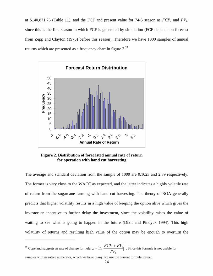
at $140,871.76 (Table 11), and the FCF and present value for 74-5 season as FCF1 and PV1,

since this is the first season in which FCF is generated by simulation (FCF depends on forecast

from Zepp and Clayton (1975) before this season). Therefore we have 1000 samples of annual

returns which are presented as a frequency chart in figure 2.27

Forecast Return Distribution

05

101520253035404550

-7 -5.8 -4.6 -3.4 -2.2 -1 0.2 1.4 2.6 3.8 5 6.2

Annual Rate of Return

Freq

uenc

y

Figure 2. Distribution of forecasted annual rate of return for operation with hand cut harvesting

The average and standard deviation from the sample of 1000 are 0.1023 and 2.39 respectively.

The former is very close to the WACC as expected, and the latter indicates a highly volatile rate

of return from the sugarcane farming with hand cut harvesting. The theory of ROA generally

predicts that higher volatility results in a high value of keeping the option alive which gives the

investor an incentive to further delay the investment, since the volatility raises the value of

waiting to see what is going to happen in the future (Dixit and Pindyck 1994). This high

volatility of returns and resulting high value of the option may be enough to overturn the

24

27 Copeland suggests as rate of change formula: ⎥⎦

⎤⎢⎣

⎡ +=

0

11lnPV

PVFCFz . Since this formula is not usable for

samples with negative numerator, which we have many, we use the current formula instead.

conclusion from the NPV approach, that is, the farmer should have already switched to

mechanized operation in 72-3 season.

Option value computation

In this section we calculate value of the mechanization option for the Florida sugarcane farmer.

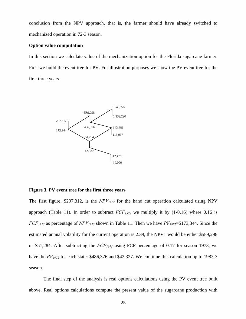
First we build the event tree for PV. For illustration purposes we show the PV event tree for the

first three years.

207,312

10,090

12,479

115,937

143,481

1,332,220

1,648,725

486,376

589,298

51,284

173,844

42,327

Figure 3. PV event tree for the first three years

The first figure, $207,312, is the NPV1972 for the hand cut operation calculated using NPV

approach (Table 11). In order to subtract FCF1972 we multiply it by (1-0.16) where 0.16 is

FCF1972 as percentage of NPV1972 shown in Table 11. Then we have PV1972=$173,844. Since the

estimated annual volatility for the current operation is 2.39, the NPV1 would be either $589,298

or $51,284. After subtracting the FCF1973 using FCF percentage of 0.17 for season 1973, we

have the PV1972 for each state: $486,376 and $42,327. We continue this calculation up to 1982-3

season.

The final step of the analysis is real options calculations using the PV event tree built

above. Real options calculations compute the present value of the sugarcane production with

25

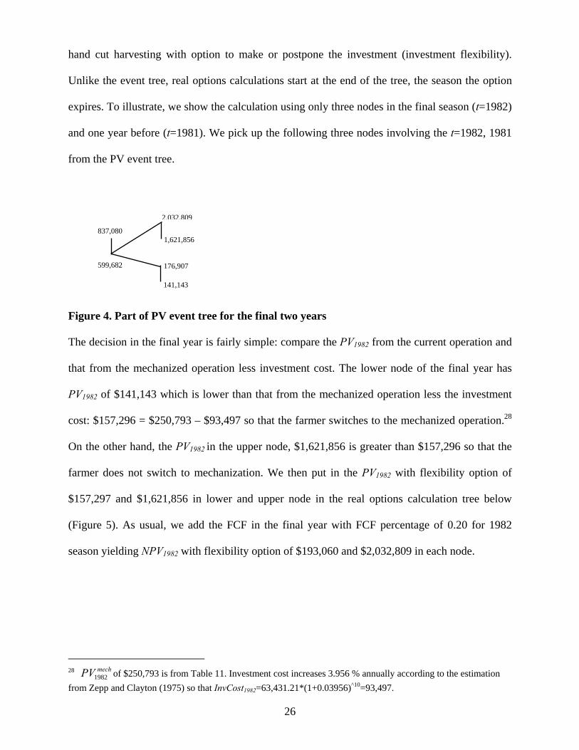
hand cut harvesting with option to make or postpone the investment (investment flexibility).

Unlike the event tree, real options calculations start at the end of the tree, the season the option

expires. To illustrate, we show the calculation using only three nodes in the final season (t=1982)

and one year before (t=1981). We pick up the following three nodes involving the t=1982, 1981

from the PV event tree.

141,143

176,907

1,621,856

2,032,809

599,682

837,080

Figure 4. Part of PV event tree for the final two years

The decision in the final year is fairly simple: compare the PV1982 from the current operation and

that from the mechanized operation less investment cost. The lower node of the final year has

PV1982 of $141,143 which is lower than that from the mechanized operation less the investment

cost: $157,296 = $250,793 – $93,497 so that the farmer switches to the mechanized operation.28

On the other hand, the PV1982 in the upper node, $1,621,856 is greater than $157,296 so that the

farmer does not switch to mechanization. We then put in the PV1982 with flexibility option of

$157,297 and $1,621,856 in lower and upper node in the real options calculation tree below

(Figure 5). As usual, we add the FCF in the final year with FCF percentage of 0.20 for 1982

season yielding NPV1982 with flexibility option of $193,060 and $2,032,809 in each node.

28 of $250,793 is from Table 11. Investment cost increases 3.956 % annually according to the estimation from Zepp and Clayton (1975) so that InvCost

mechPV1982

1982=63,431.21*(1+0.03956)^10=93,497.

26

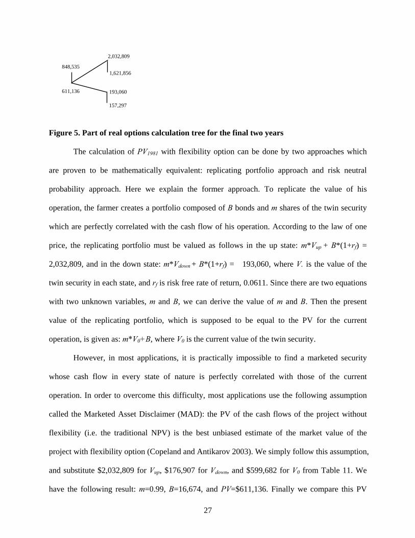
2,032,809

157,297

193,060

1,621,856

611,136

848,535

Figure 5. Part of real options calculation tree for the final two years

The calculation of PV1981 with flexibility option can be done by two approaches which

are proven to be mathematically equivalent: replicating portfolio approach and risk neutral

probability approach. Here we explain the former approach. To replicate the value of his

operation, the farmer creates a portfolio composed of B bonds and m shares of the twin security

which are perfectly correlated with the cash flow of his operation. According to the law of one

price, the replicating portfolio must be valued as follows in the up state: m*Vup + B*(1+rf) =

2,032,809, and in the down state: m*Vdown + B*(1+rf) = 193,060, where V. is the value of the

twin security in each state, and rf is risk free rate of return, 0.0611. Since there are two equations

with two unknown variables, m and B, we can derive the value of m and B. Then the present

value of the replicating portfolio, which is supposed to be equal to the PV for the current

operation, is given as: m*V0+B, where V0 is the current value of the twin security.

However, in most applications, it is practically impossible to find a marketed security

whose cash flow in every state of nature is perfectly correlated with those of the current

operation. In order to overcome this difficulty, most applications use the following assumption

called the Marketed Asset Disclaimer (MAD): the PV of the cash flows of the project without

flexibility (i.e. the traditional NPV) is the best unbiased estimate of the market value of the

project with flexibility option (Copeland and Antikarov 2003). We simply follow this assumption,

and substitute $2,032,809 for Vup, $176,907 for Vdown, and $599,682 for V0 from Table 11. We

have the following result: m=0.99, B=16,674, and PV=$611,136. Finally we compare this PV

27

and PV for mechanized operation less investment cost: PV1981 = Max[$611,136,

$252,823-$89,939] = $611,136 so that the farmer retains the current operation. As usual we add

FCF1981 for the year to compute NPV1981, yielding the NPV1981 with flexibility option of

$848,535 for this node. We repeat these steps for other nodes of season 82-3 and 81-2, and up to

season 72-3, and computed the NPV1972 with option value = $396,009.

Then the option value is simply calculated as: (NPV1972 with option value) - NPV1972 =

$396,009 - $207,312 = $188,697 = OptValue1972 which is the value of option to make or

postpone the investment (investment flexibility). Since making investment at that time means

exercising the option to invest, the farmer loses the option value of flexibility at the same time.

The farmer would not make an investment until it is profitable enough to overcome the loss of

option value to wait. Therefore the decision rule of investment for the farmer is “invest if NPV of

mechanized operation less investment cost and option value is greater than NPV of the current

operation”. The calculation is given as: $357,966 -

$63,431 - $188,697 = $105,837 < $207,312 = .

=−− 197219721972 OptValueInvCostNPV mech

1972NPV

The conclusion from the ROA is that the farmer must not switch to mechanized operation

in 72-3 season, which is the exact opposite conclusion to that suggested by the traditional NPV

approach. Since the sugarcane farmers in Florida are exposed to highly volatile FCF, the value of

keeping the flexibility option alive is very high, enough to overturn the conclusion from the

traditional NPV approach. As the theory of ROA shows, high volatility of FCF gives the

investors incentive to wait until the uncertainty resolves. The ROA correctly predicts that

average farmers would not have invested in mechanization in 72-3 season.

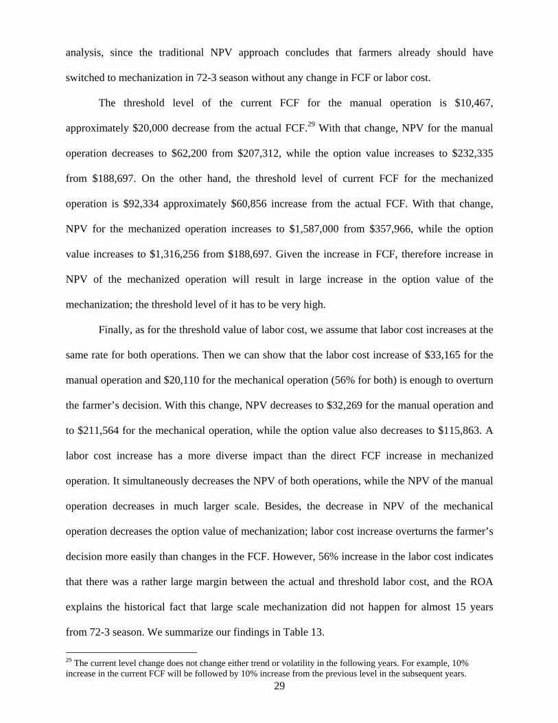
Threshold value of FCF and labor cost

The final question for the current study is how much FCF decrease (FCF decrease in hand

harvesting or FCF increase in mechanical harvesting) and labor cost increase would have been

enough to force average farmers to switch to mechanization in 72-3 season. We use ROA for this

28

analysis, since the traditional NPV approach concludes that farmers already should have

switched to mechanization in 72-3 season without any change in FCF or labor cost.

The threshold level of the current FCF for the manual operation is $10,467,

approximately $20,000 decrease from the actual FCF.29 With that change, NPV for the manual

operation decreases to $62,200 from $207,312, while the option value increases to $232,335

from $188,697. On the other hand, the threshold level of current FCF for the mechanized

operation is $92,334 approximately $60,856 increase from the actual FCF. With that change,

NPV for the mechanized operation increases to $1,587,000 from $357,966, while the option

value increases to $1,316,256 from $188,697. Given the increase in FCF, therefore increase in

NPV of the mechanized operation will result in large increase in the option value of the

mechanization; the threshold level of it has to be very high.

Finally, as for the threshold value of labor cost, we assume that labor cost increases at the

same rate for both operations. Then we can show that the labor cost increase of $33,165 for the

manual operation and $20,110 for the mechanical operation (56% for both) is enough to overturn

the farmer’s decision. With this change, NPV decreases to $32,269 for the manual operation and

to $211,564 for the mechanical operation, while the option value also decreases to $115,863. A

labor cost increase has a more diverse impact than the direct FCF increase in mechanized

operation. It simultaneously decreases the NPV of both operations, while the NPV of the manual

operation decreases in much larger scale. Besides, the decrease in NPV of the mechanical

operation decreases the option value of mechanization; labor cost increase overturns the farmer’s

decision more easily than changes in the FCF. However, 56% increase in the labor cost indicates

that there was a rather large margin between the actual and threshold labor cost, and the ROA

explains the historical fact that large scale mechanization did not happen for almost 15 years

from 72-3 season. We summarize our findings in Table 13.

29

29 The current level change does not change either trend or volatility in the following years. For example, 10% increase in the current FCF will be followed by 10% increase from the previous level in the subsequent years.

Table 13. The threshold level of FCF and labor cost ($) Threshold level

(actual level)Resulting NPV

(actual NPV)Resulting option value

(actual option value)FCF decrease for

manual op. 10,467

(30,467)62,200

(207,312)232,335

(188,697)FCF increase for mechanical op.

92,334 (31,478)

1,587,000 (357,966)

1,316,256 (188,697)

92,181 (59,016)

for manual op.

32,269 (207,312)

for manual op.56% labor cost

increase for both operations 55,894

(35,784) for mechanical op.

211,564 (357,966)

for mechanical op.

115,863 (188,697)

Concluding remarks

Previous studies of Florida sugarcane production, which compared the cost and returns

from mechanically harvested operations with those of hand cutting operations (Zepp and Clayton

1975, Zepp 1975, Walker 1972), found the cost advantage of the former as early as 1972-3

season. Although this cost advantage is offset by reduced revenue due to large field losses and

higher trash content with mechanical harvesting for 1972-3 season, projected 1974-75 machinery

operating rates and additional 10% labor cost increase would have been sufficient to give the net

returns advantage to the mechanical operation (Zepp 1975). However, the historical fact shows

that the large scale mechanization investment did not happen until mid- and late 1980s, as long

as 15 years from 1972-3 season. Using the data provided by these authors, the current study

analyzes the dynamic decision making process of farmers with the two methodologies: net

present value (NPV) approach and real options approach (ROA).

The NPV approach supports the views of previous researches: NPV less initial

investment cost of mechanization ($294,534) exceeds the NPV for operation with hand cut

harvesting ($207,312), suggesting that the model farmer should have switched to mechanized

operation even in 72-3 season. Then again, the methodology fails to explain the fact that only

15% of sugarcane was harvested by machine for 1972-3 season. The conclusion from the ROA is

exactly opposite to that from the NPV approach. Since the sugarcane farmers in Florida are

30

exposed to highly volatile FCF (volatility of annual rate of return = 2.39), the value of keeping

the flexibility option alive is very high, enough to overturn the NPV conclusion. Our calculation

shows that the option value of investment opportunity is $188,697. As a result, NPV less

investment cost and option value is $105,837 which is lower than NPV for the manual operation

($207,312).

Threshold level analysis shows, for the immediate investment, it takes more than $20,000

decrease in the current FCF for the manual operation or $60,000 increase in the current FCF for

the mechanical operation. The analysis also shows that a 56% increase in the labor cost for both

operations is also enough for the immediate mechanization. All three figures indicate that there

was a rather large margin between the actual and threshold level, and the ROA explains the

historical fact that large scale mechanization did not happen for as long as 15 years from 72-3

season.

References

ARMS, Economic Research Service, U.S. Department of Agriculture, Washington, DC. http://www.ers.usda.gov/Data/ARMS/app/Farm.aspx. Brockwell, J. B. and R. A. Davis. Time Series: Theory and Methods. Springer-Verlag (1991). Brockwell, J. B. and R. A. Davis. Introduction to Time Series and Forecasting. Springer-Verlag (2002). Carey J. M. and D. Zilberman, “A Model of Investment under Uncertainty: Modern Irrigation Technology and Emerging Markets in Water,” American Journal of Agricultural Economics, 84(1) (2002): 171-83. Copeland, T. and V. Antikarov. Real Options: A Practioner’s Guide. Texere (2003). Copeland, T., T. Koller, and J. Murrin. Valuation: Measuring and Managing the Value of Companies. John Wiley and Sons (1994). Dixit, A.K., and R.S. Pindyck. Investment under Uncertainty. Princeton University Press (1994). Emerson, R.D. “Agricultural Labor Markets and Immigration.” Choices. 22(1),1st Qtr, 2007. Engel, P. D. and J. Hyde “A Real Options Analysis of Automatic Milking Systems,” Agricultural and Resource Economics Review, 32(2) (2003): 282-94. Florida Agricultural Statistics. Field Crops Summary. NASS, U.S. Department of Agriculture, (various years).

31

Internal Revenue Service. Statistics of Income – 2004. Corporate Income Tax Returns, Washington, DC. (2007). Iwai, N., R. D. Emerson, and L. M. Walters. “Legal Status and U.S. Farm Wages.” Southern Agricultural Economics Association Annual Meeting, Orlando, Florida, (February 2006). Ise, S. and J.M. Perloff. “Legal Status and Earnings of Agricultural Workers,” American Journal of Agricultural Economics, 77 (1995): 375-86. Kijima, M. Introduction to Financial Engineering II: Theory of Derivatives Pricing. Nikkagiren (1994). Kobayashi, Y. Derivatives and Real Option. Chuo Keizai Sha (2003). Napasintuwong, O. and R.D. Emerson. “Labor Substitutability in Labor Intensive Agriculture and Technological Change in the Presence of Foreign Labor,” Selected Paper, American Agricultural Economics Association Annual Meeting, Denver, Colorado (August 2004). Preston, Julia. “Short on Labor, Farmers in U.S. Shift to Mexico,” The New York Times, September 5, 2007. Samuelson, P. “Proof that Properly Anticipated Prices Fluctuate Randomly,” Industrial Management Review 6(2) (1965): 41-9. Taylor, J.E. “Earnings and Mobility of Legal and Illegal Immigrant Workers in Agriculture,” American Journal of Agricultural Economics, 74 (1992): 889-96. Trigeorgis, L. Real Options: Managerial Flexibility and Strategy in Resource Allocation. MIT Press (1996). U.S. Department of Agriculture. Florida Sugarcane Production Costs. Administrative Records. Washington, DC. U.S. Department of Labor. Florida Sugarcane Labor Costs. Administrative Records. Washington, DC. U.S. Department of Labor. Annual Reports. OWS, ETA. Washington, DC. (various years). Walker, C. Cost and Returns from Sugarcane in South Florida. University of Florida Cooperative Extension Service Cir. 374 (1972). Wall Street Journal. “Immigration Non-Harvest,” editorial, New York. July 20, 2007. Zepp, G.A. and J.E. Clayton. A Comparison of Costs and Returns for Hand Cutting and Mechanically Harvesting Sugarcane in Florida, 1972-73 Season. Food and Resource Economics Dept., University of Florida (1975).

Zepp, G.A. Effects of Harvest Mechanization on the Demand for Labor in Florida Sugarcane Industry. Food and Resource Economics Dept., University of Florida (1975).

32