Exporting  data  from  DataStudio  

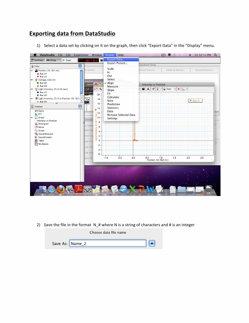
1) Select  a  data  set  by  clicking  on  it  on  the  graph,  then  click  “Export  Data”  in  the  “Display”  menu.  

 

 

 

2) Save  the  file  in  the  format    N_#  where  N  is  a  string  of  characters  and  #  is  an  integer    

 

 

 

 

 

 

 

Graphing  data  in  Igor  Pro  

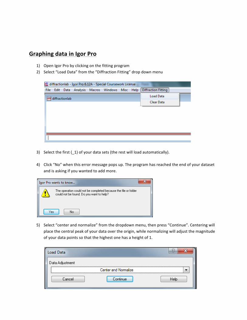
1) Open  Igor  Pro  by  clicking  on  the  fitting  program  2) Select  “Load  Data”  from  the  “Diffraction  Fitting”  drop  down  menu    

 

   

3) Select  the  first  (_1)  of  your  data  sets  (the  rest  will  load  automatically).      

4) Click  “No”  when  this  error  message  pops  up.  The  program  has  reached  the  end  of  your  dataset  and  is  asking  if  you  wanted  to  add  more.    

 

5) Select  “center  and  normalize”  from  the  dropdown  menu,  then  press  “Continue”.  Centering  will  place  the  central  peak  of  your  data  over  the  origin,  while  normalizing  will  adjust  the  magnitude  of  your  data  points  so  that  the  highest  one  has  a  height  of  1.      

 

6) Set  the  parameters  of  your  fit.  If  the  check  box  next  to  a  cell  is  checked,  that  value  will  be  fixed  for  the  fit.  If  the  check  box  is  left  empty,  the  fitting  program  will  use  your  input  as  a  beginning  estimate  but  will  change  it  as  necessary  to  make  a  good  fit.  -­‐ “Number  of  slits”  is  simply  the  number  of  slits  used  for  this  particular  dataset    -­‐ “Intensity0(%)”  is  the  intensity  of  your  lowest  data  point.  Optimistically  this  should  be  zero,  

so  put  “0”  in  the  field  but  leave  the  check  box  unchecked    -­‐ “x0  (cm)”  is  the  distance  of  the  peak  of  your  data  from  the  origin.  This  was  set  to  be  

approximately  0,  but  the  centering  program  is  not  perfect.  Thus,  you  should  set  this  value  to  “0”  but  leave  the  box  unchecked.  

-­‐ “Intensity(%)”  is    the  intensity  of  your  highest  data  point.  Since  we  normalized  this  data,  we  know  this  is  1.  Enter  “1”  in  the  field  and  check  the  box  to  fix  the  value.    

-­‐ “Wavelength(nm)”  is  the  wavelength  of  laser  light  used  in  the  experiment.  Since  we  know  this  value,  enter  it  and  check  the  check  box  to  fix  it.    

-­‐ “Distance(cm)”  is  the  distance  from  the  slits  to  the  aperture  on  the  light  sensor.  Since  we  know  this  value,  enter  it  and  check  the  check  box  to  fix  it.  

-­‐ “Slit  Width(mm)”  is  the  width  between  the  slits  you  are  using.  This  is  the  value  you  are  usually  trying  to  calculate,  so  we  do  not  want  to  fix  it.  However,  entering  a  guess  (perhaps  motivated  by  the  label  on  the  slits  that  tells  you  the  width!)  will  help  the  fitting  program  obtain  a  better  fit.    

-­‐ “Slit  Separation  (mm)”  is  the  separation  between  the  slits  you  are  using.  Similarly  to  the  width,    we  are  often  trying  to  calculate  this  value,  so  input  a  guess  but  do  not  fix  the  value.  

 

   

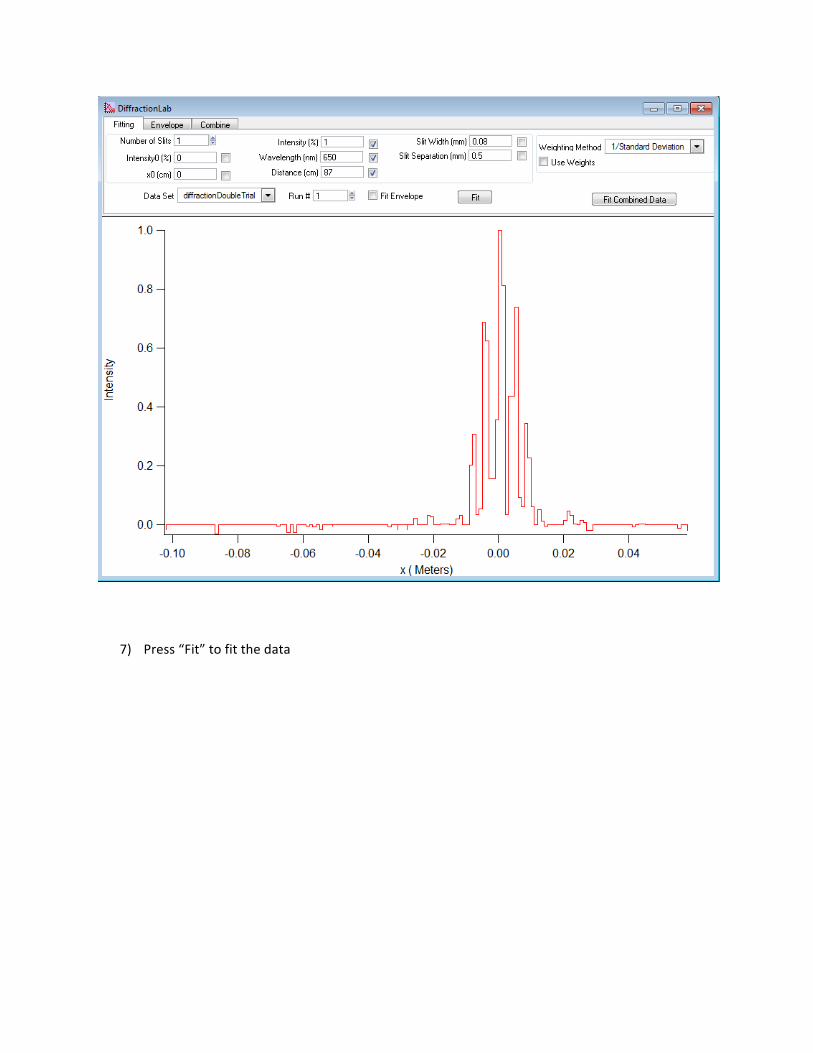
7) Press  “Fit”  to  fit  the  data  

   

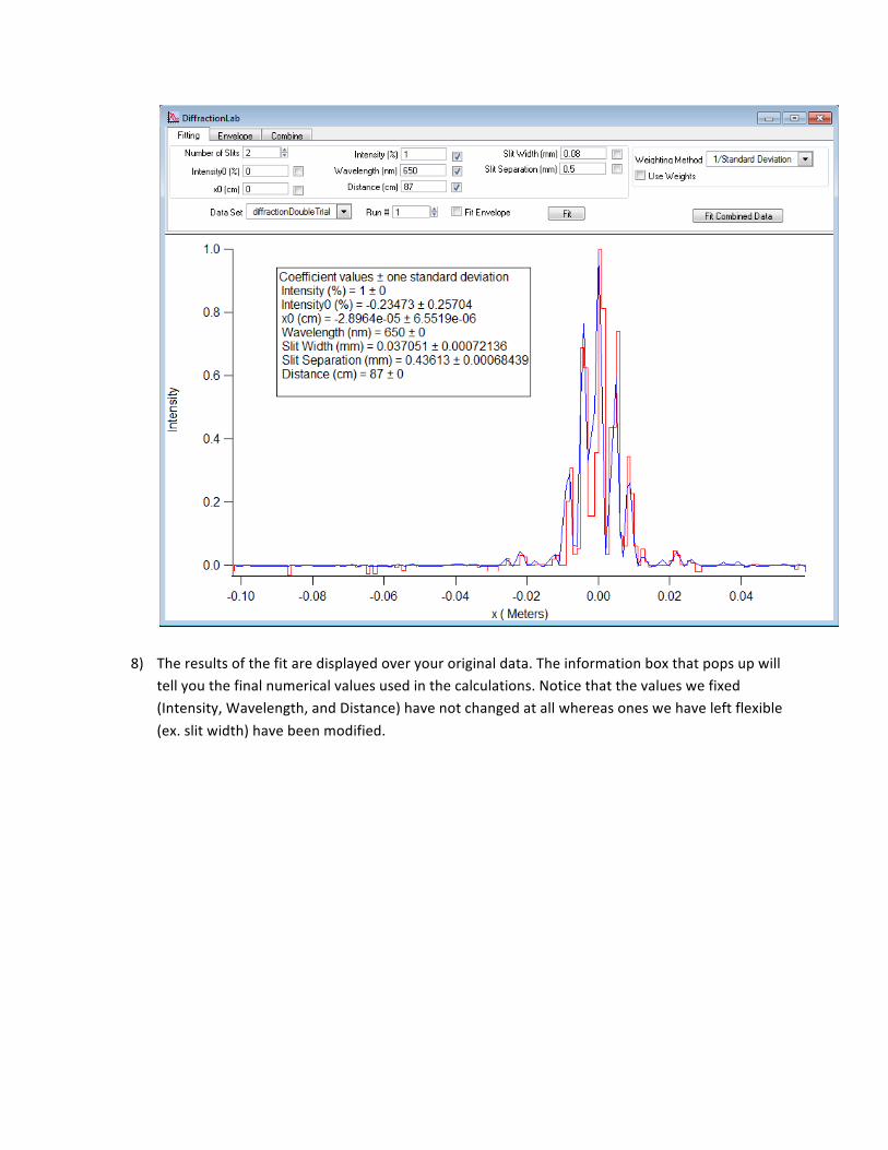
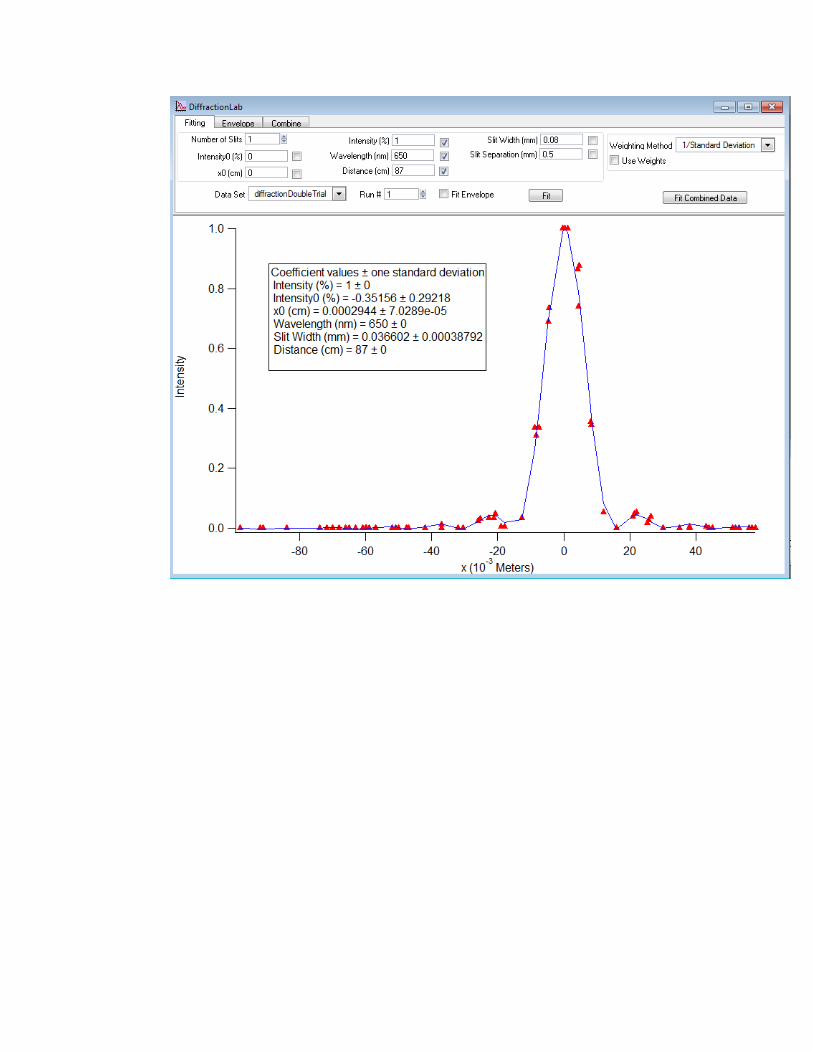
8) The  results  of  the  fit  are  displayed  over  your  original  data.  The  information  box  that  pops  up  will  tell  you  the  final  numerical  values  used  in  the  calculations.  Notice  that  the  values  we  fixed  (Intensity,  Wavelength,  and  Distance)  have  not  changed  at  all  whereas  ones  we  have  left  flexible  (ex.  slit  width)  have  been  modified.    

 

 

 

 

 

 

 

 

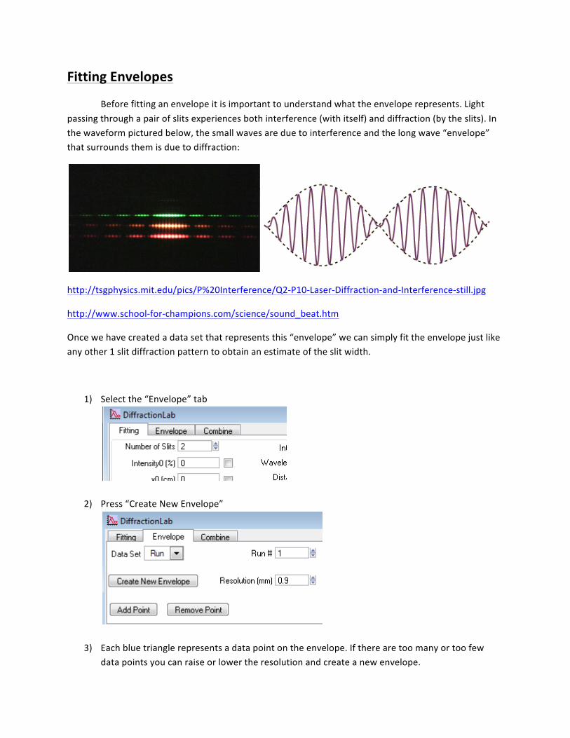
Fitting  Envelopes  

Before  fitting  an  envelope  it  is  important  to  understand  what  the  envelope  represents.  Light  passing  through  a  pair  of  slits  experiences  both  interference  (with  itself)  and  diffraction  (by  the  slits).  In  the  waveform  pictured  below,  the  small  waves  are  due  to  interference  and  the  long  wave  “envelope”  that  surrounds  them  is  due  to  diffraction:  

 

http://tsgphysics.mit.edu/pics/P%20Interference/Q2-­‐P10-­‐Laser-­‐Diffraction-­‐and-­‐Interference-­‐still.jpg  

http://www.school-­‐for-­‐champions.com/science/sound_beat.htm  

Once  we  have  created  a  data  set  that  represents  this  “envelope”  we  can  simply  fit  the  envelope  just  like  any  other  1  slit  diffraction  pattern  to  obtain  an  estimate  of  the  slit  width.    

 

1) Select  the  “Envelope”  tab  

   

2) Press  “Create  New  Envelope”  

   

3) Each  blue  triangle  represents  a  data  point  on  the  envelope.  If  there  are  too  many  or  too  few  data  points  you  can  raise  or  lower  the  resolution  and  create  a  new  envelope.    

   

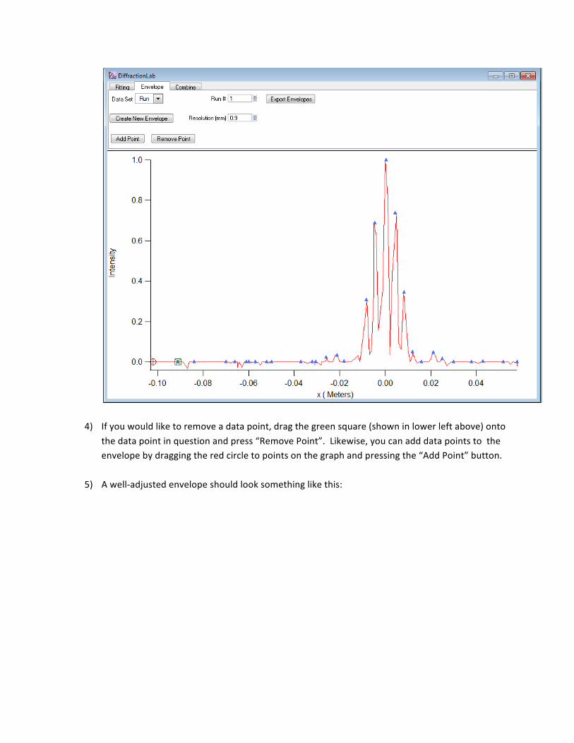
4) If  you  would  like  to  remove  a  data  point,  drag  the  green  square  (shown  in  lower  left  above)  onto  the  data  point  in  question  and  press  “Remove  Point”.    Likewise,  you  can  add  data  points  to    the  envelope  by  dragging  the  red  circle  to  points  on  the  graph  and  pressing  the  “Add  Point”  button.      

5) A  well-­‐adjusted  envelope  should  look  something  like  this:          

   

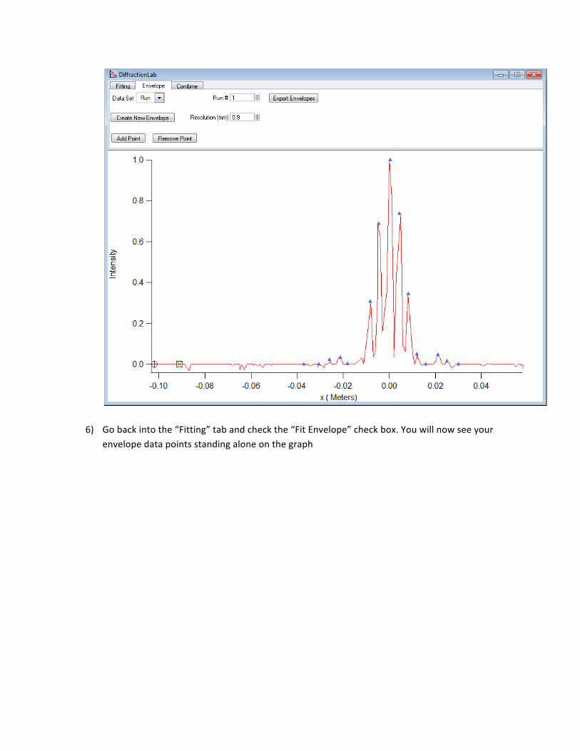
6) Go  back  into  the  “Fitting”  tab  and  check  the  “Fit  Envelope”  check  box.  You  will  now  see  your  envelope  data  points  standing  alone  on  the  graph  

   

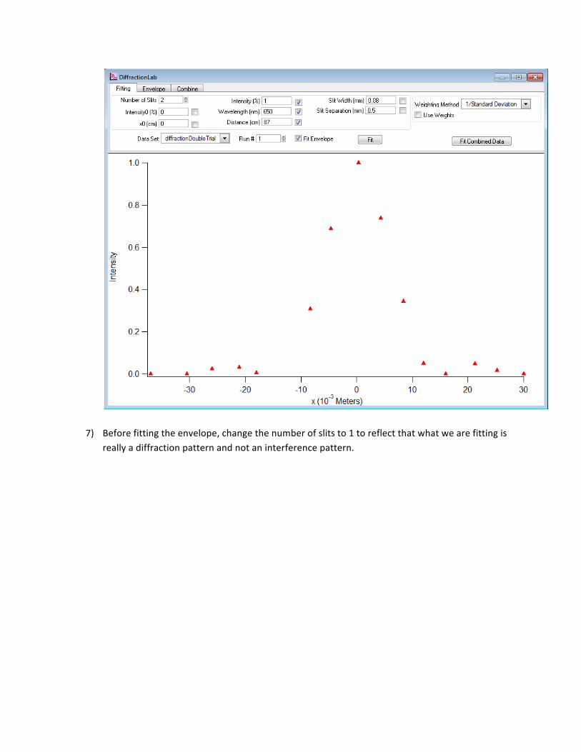
7) Before  fitting  the  envelope,  change  the  number  of  slits  to  1  to  reflect  that  what  we  are  fitting  is  really  a  diffraction  pattern  and  not  an  interference  pattern.      

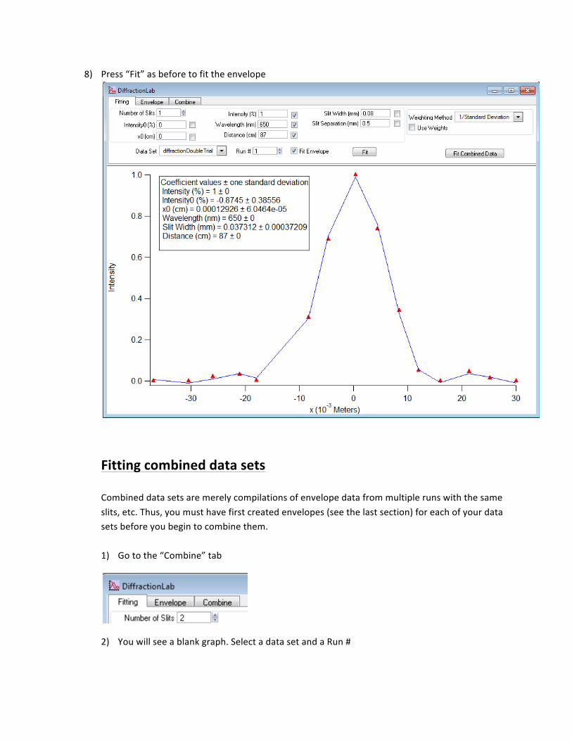
8) Press  “Fit”  as  before  to  fit  the  envelope    

   

 Fitting  combined  data  sets      Combined  data  sets  are  merely  compilations  of  envelope  data  from  multiple  runs  with  the  same  slits,  etc.  Thus,  you  must  have  first  created  envelopes  (see  the  last  section)  for  each  of  your  data  sets  before  you  begin  to  combine  them.      1) Go  to  the  “Combine”  tab    

   

2) You  will  see  a  blank  graph.  Select  a  data  set  and  a  Run  #      

   

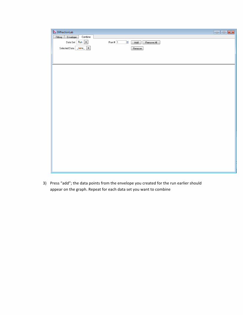
3) Press  “add”;  the  data  points  from  the  envelope  you  created  for  the  run  earlier  should  appear  on  the  graph.  Repeat  for  each  data  set  you  want  to  combine      

   

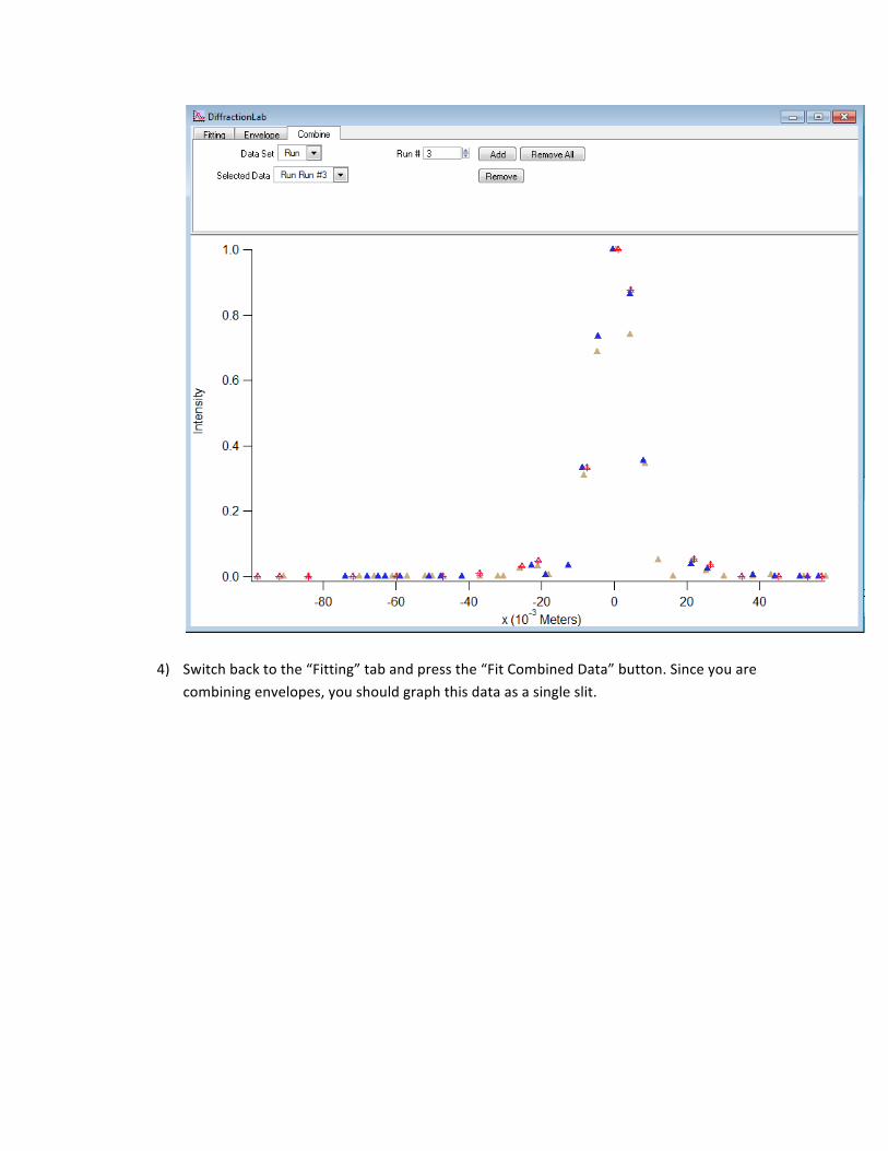
4) Switch  back  to  the  “Fitting”  tab  and  press  the  “Fit  Combined  Data”  button.  Since  you  are  combining  envelopes,  you  should  graph  this  data  as  a  single  slit.