Lab Manual Excel Module - University of...

Lab manual for Peeking into Computer Science 2nd Ed by Jalal Kawash. http://pages.cpsc.ucalgary.ca/~kawash/peeking.html

Lab Manual

Excel Module


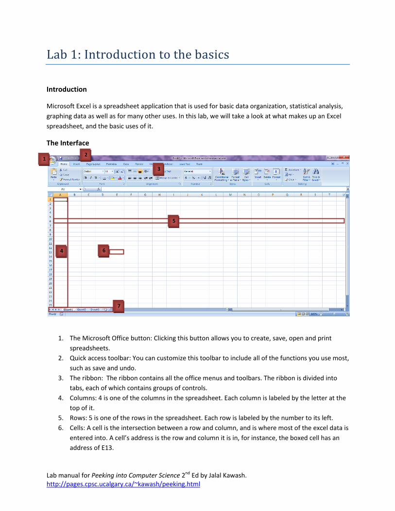
Lab 1: Introduction to the basics

Introduction

Microsoft Excel is a spreadsheet application that is used for basic data organization, statistical analysis,

graphing data as well as for many other uses. In this lab, we will take a look at what makes up an Excel

spreadsheet, and the basic uses of it.

The Interface

1. The Microsoft Office button: Clicking this button allows you to create, save, open and print

spreadsheets.

2. Quick access toolbar: You can customize this toolbar to include all of the functions you use most,

such as save and undo.

3. The ribbon: The ribbon contains all the office menus and toolbars. The ribbon is divided into

tabs, each of which contains groups of controls.

4. Columns: 4 is one of the columns in the spreadsheet. Each column is labeled by the letter at the

top of it.

5. Rows: 5 is one of the rows in the spreadsheet. Each row is labeled by the number to its left.

6. Cells: A cell is the intersection between a row and column, and is where most of the excel data is

entered into. A cell’s address is the row and column it is in, for instance, the boxed cell has an

address of E13.

1 2

3

6

5

4

7

s


7. The worksheet toolbar: This toolbar allows you to move between the different sheets in a

workbook. It also allows you to create new worksheets.

Exercise 1

1. Enter the data “Sunday” into cell A1 and “Monday” into cell B2.

2. Type in “17/08” into cell E8.

3. Type in “2” into cell I8 and “4” into cell I9.

Auto-complete

Your worksheet should now look like this:

Notice how Excel automatically detected that 17/08 was a date and converted it into 17-Aug. We

will discuss formatting data later on in this lab.

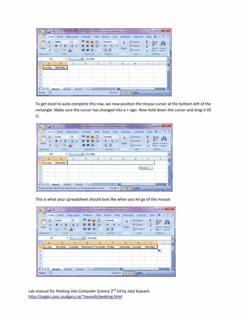
Now we want to select both cells A1 and B1 together. To do this, click on A1 and without releasing

the mouse button, move over cell B2. Now there should be a rectangle around both cells as shown

below.


To get excel to auto-complete this row, we now position the mouse cursor at the bottom-left of the

rectangle. Make sure the cursor has changed into a + sign. Now hold down the cursor and drag it till

I1.

This is what your spreadsheet should look like when you let go of the mouse:


Exercise 2

1. Auto-complete cells I8 and I9 all the way to I14.

2. Auto-complete cell E8 all the way to E12.

Formatting

Excel allows you to format your data so that it shows up in the way you need it to. Let us start with

number formatting. Select cells I8 and I9. If you take a look at the Number group in the Home tab

on the ribbon, you will notice that the current number format is “General”.

Selecting that drop down box shows you some of the available number formats, shown below.


Select currency from the drop down menu. Now you will notice that the two numbers have a $ sign

preceding them, and have two decimal places. Let us change the currency symbol to a Euro. Select

the Euro symbol from the currency format menu.

Exercise 3

Modify cells I8 and I9 by removing the 2 decimal places.

Exercise 4

Format cell E8 so that it looks like August 17, 2010.

Basic Calculations

When working on a spreadsheet, you will almost definitely need to perform some calculations on

the data you have. The first thing you need to remember about Excel calculations is that formulas

always start with an = sign. Let us begin with a very simple calculation. Type “=3+5” into cell A5 as

shown below.


Press Enter. Excel automatically replaces the formula with the result of the equation. Note that Excel

formulas follow the order of operations.

Now let us calculate the sum of the numbers in I8 and I9. In cell J10, type “=I8+I9”. One other option

is to type in “=”, then select cell I8. After than type in “+” then select I9.


Pressing Enter will give you the result of the calculation. Double-clicking on the cell with the formula

allows you to edit the formula.

Excel has built-in functions that make your life easier. One of them is the SUM function. In cell J11,

type “=sum(“. Now select both cells I8 and I9.

Pressing Enter gives you the same result as the plus operation we did in cell J10. Try changing cell I8

and notice how the change is reflected in both formulas.

Exercise 5

1. Open Sheet 2 in your workbook.

2. In cells A1 and A2, type in 1000 and 1500 respectively.

3. Use auto-complete to fill in cells A3 to A8.

4. Format the numbers so that they show the 1000 separator (1,000) and have one decimal place.

5. Calculate the following values for cells A1 to A8 using built-in Excel functions:

a. Sum

b. Maximum

c. Minimum

d. Average

e. Median

f. Standard deviation

6. Enter the number 5000 into cell A9 and modify all the above formulas to include it.

7. Calculate the sum of the Maximum and Minimum, and then divide this number by the standard

deviation.

Lab Manual Excel Module - University of...

Documents

Transcript of Lab Manual Excel Module - University of...