Distributed Intelligent Systems and Algorithms Laboratory EPFL

JNP, Lab 7: Introduction to Webots and Sensor Modeling 1

Lab 7: Introduction to Webots and Sensor Modeling

This laboratory requires the following software: • Webots simulator • C development tools (gcc, make, etc.) The laboratory duration is approximately 3 hours. Although this laboratory is not

graded, we encourage you to take your own personal notes as the final verification test might leverage results acquired during the laboratory session. For any questions, please contact us at sis-ta@groupes.epfl.ch.

1.1 Information In this assignment, you will find several exercises and questions. • Sx means that the question can be solved using only additional simulation. • Qx means that the question can be answered theoretically, without any

simulation. • Ix means that the problem has to be solved by implementing some code and

performing a simulation. • Bx means that the question is optional and should be answered if you have

enough time at your disposal.

1.2 Getting Started (Short reminder) To start with this lab, you will need to boot to Ubuntu and download the material

available on Moodle. Download lab07.tar.gz in your personal directory. Now, extract the lab archive (you can type in the terminal: tar xvfz lab07.tar.gz.)

2 Introduction

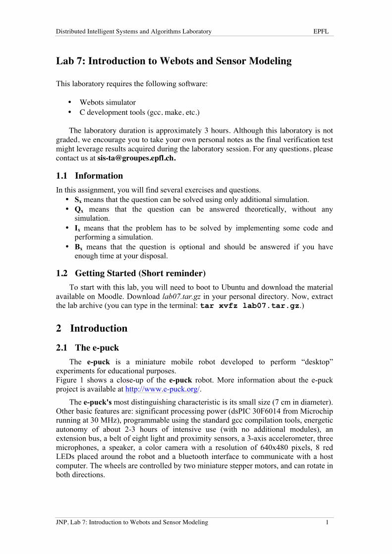
2.1 The e-puck The e-puck is a miniature mobile robot developed to perform “desktop”

experiments for educational purposes. Figure 1 shows a close-up of the e-puck robot. More information about the e-puck project is available at http://www.e-puck.org/.

The e-puck's most distinguishing characteristic is its small size (7 cm in diameter). Other basic features are: significant processing power (dsPIC 30F6014 from Microchip running at 30 MHz), programmable using the standard gcc compilation tools, energetic autonomy of about 2-3 hours of intensive use (with no additional modules), an extension bus, a belt of eight light and proximity sensors, a 3-axis accelerometer, three microphones, a speaker, a color camera with a resolution of 640x480 pixels, 8 red LEDs placed around the robot and a bluetooth interface to communicate with a host computer. The wheels are controlled by two miniature stepper motors, and can rotate in both directions.

Distributed Intelligent Systems and Algorithms Laboratory EPFL

JNP, Lab 7: Introduction to Webots and Sensor Modeling 2

Figure 1: Close-up of an e-puck robot.

The simple geometrical shape along with the positioning of the motors allows the e-puck to negotiate any kind of obstacle or corner.

Modularity is another characteristic of the e-puck robot. Each robot can be extended by adding a variety of modules. A follow-up lab on the real e-puck (next week) will allow you to further understand the e-puck hardware platform.

2.2 Webots Webots is a fast prototyping and simulation software developed by Cyberbotics

Ltd., a spin-off company ofEPFL. Webots allows the experimenter to design, program, and simulate virtual robots which act and sense in a 3D environment.

Webots can either simulate the physics of the world and the robots (nonlinear friction, slipping, mass distribution, etc.) or simply kinematic laws. The choice of the level of simulation is a trade-off between simulation speed and simulation realism. However, all sensors and actuators are affected by a realistic amount of noise so that the transfer from simulation to the real robot is usually quite smooth.

Many types of robots can be simulated with Webots, including wheeled, legged, flying, and swimming robots. Some interesting examples can be found in the Webots Guided Tour (menu: Help->Webots Guided Tour).

The image cannot be displayed. Your computer may not have enough memory to open the image, or the image may have been corrupted. Restart your computer, and then open the file again. If the red x still appears, you may have to delete the image and then insert it again.

Distributed Intelligent Systems and Algorithms Laboratory EPFL

JNP, Lab 7: Introduction to Webots and Sensor Modeling 3

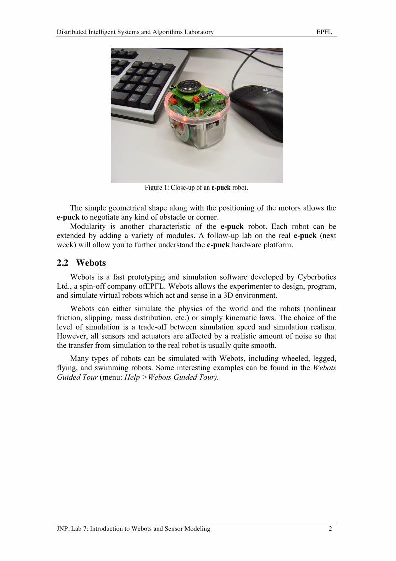
Figure 2:. Webots simulation of the e-puck robot.

A simulated model of the e-puck robot is provided with Webots (see Figure 2). The current version of the e-puck model simulates the differential-drive system with physics (including friction, collision detection, etc.), the distance sensors, the leds, the accelerometer, the light sensors, and the camera. In the future, this model will be further refined to simulate more of the e-puck's functionality. During this laboratory we will perform experiments exclusively with simulated e-puck models.

There are two Webots help sources available online as a PDF and HTML: Webots User Guide and Webots Reference Manual. You can access them at the following link: http://www.cyberbotics.com/documentation.php or directly from the Help menu of Webots.

3 Webots mini-tutorial

3.1 Starting Webots 1. Launch Webots from a terminal by entering this command:

webots --mode=pause &

2. If you're opening Webots for the first time, the Welcome screen will show up: you can have a look at the Guided Tour if you want. Otherwise, just click on the close button.

3. From the menu, select File->Open World, and choose the e-puck.wbt file from the lab_07/worlds directory structure that was just created.

4. At this point the e-puck model should appear in Webots main window.

5. Now you can build the project by clicking on the Build button:

Distributed Intelligent Systems and Algorithms Laboratory EPFL

JNP, Lab 7: Introduction to Webots and Sensor Modeling 4

6. Now you can hit the Run button and the simulation will start. Note that the robot is not supposed to move at this point.

You can Stop, Run and Revert the simulation with the corresponding buttons in the

Webots toolbar. Please try pressing all these buttons to see what they do:

§ Revert: Reloads the world (.wbt file) and restarts the simulation from the beginning

§ Step: Executes one simulation step

§ Pause: Stops at the current simulation step

§ Run real-time: Runs the simulation

§ Run: Runs the simulation

§ Run fast: Runs the simulation at the maximal CPU speed (Only visual rendering is disabled for better performance)

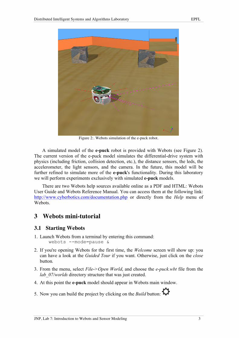
Next to these buttons you will see two numerical indicators (see Figure 3): The left

indicator (a clock like 0:02:48:320) shows the simulation elapsed time as Hours:Minutes:Seconds:Milliseconds. Note that this is simulated time (rather than the wall-clock time) emulating faithfully the potential real time progress that would be expected if the experiment was carried out in reality. It stops when the simulation is stopped.

Figure 3: Elapsed time indicator and speedometer

The right indicator (3.11x) is the speedometer which indicates how fast the simulation is currently running with respect to real time (wall-clock time). See how the elapsed time and speedometer are affected by the Run and Fast buttons.

3.2 Manipulating objects Learn how to navigate in the 3D view using the mouse: try to drag the mouse

while pressing all possible mouse buttons (and the wheel) combinations.

Various objects can be manipulated with the mouse: This allows you to change the initial configuration, or to interact with a running simulation. In order to move an object: § Select the object and drag the green, red and blue arrows to move and rotate the

object in different axis § Select the object, hold the Shift key and drag the mouse while pressing the left

mouse button to shift an object in the xz-plane (parallel to the ground) § Select the object, hold the Shift key and drag the mouse up and down, while

pressing simultaneously the left and right mouse buttons (or the middle button), to lift and lower the object (alternatively you can also use the mouse wheel)

The image cannot be displayed. Your computer may not have enough memory to open the image, or the image may have been corrupted. Restart your computer, and then open the file again. If the red x still appears, you may have to delete the image and then insert it again.

Distributed Intelligent Systems and Algorithms Laboratory EPFL

JNP, Lab 7: Introduction to Webots and Sensor Modeling 5

§ To apply a force to an object, place the mouse pointer where the force will apply (without the object being selected), hold down the Alt and Control key and left mouse button together while dragging the mouse

§ To apply a torque to an object, place the mouse pointer on it (without the object being selected), hold down the Alt and Control key and right mouse button together while dragging the mouse.

§ Applying force and torque works only for objects with mass. In the case of the world where you are working now, only the e-puck has mass (not the boxes).

Now, if you want, you may try all of the above manipulations with the e-puck and the obstacles both while the simulation is stopped or running. The mini-tutorial is finished.

4 Simulating sensors

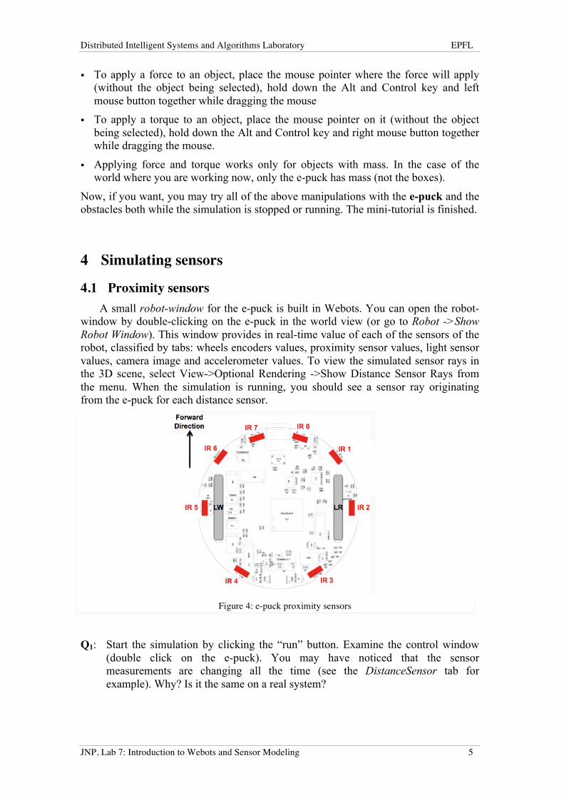
4.1 Proximity sensors A small robot-window for the e-puck is built in Webots. You can open the robot-

window by double-clicking on the e-puck in the world view (or go to Robot ->Show Robot Window). This window provides in real-time value of each of the sensors of the robot, classified by tabs: wheels encoders values, proximity sensor values, light sensor values, camera image and accelerometer values. To view the simulated sensor rays in the 3D scene, select View->Optional Rendering ->Show Distance Sensor Rays from the menu. When the simulation is running, you should see a sensor ray originating from the e-puck for each distance sensor.

Q1: Start the simulation by clicking the “run” button. Examine the control window

(double click on the e-puck). You may have noticed that the sensor measurements are changing all the time (see the DistanceSensor tab for example). Why? Is it the same on a real system?

The image cannot be displayed. Your computer may not have enough memory to open the image, or the image may have been corrupted. Restart your computer, and then open the file again. If the red x still appears, you may have to delete the image and then insert it again.

Figure 4: e-puck proximity sensors

Distributed Intelligent Systems and Algorithms Laboratory EPFL

JNP, Lab 7: Introduction to Webots and Sensor Modeling 6

S2: By moving objects around the e-puck, draw the response of the proximity sensor as a function of the distance to an obstacle. Note that the range of the e-puck’s distance sensors is fairly short.

Q3: What happens if an obstacle and the robot are interpenetrating? What are the proximity sensor measurements in this case (hint: you can use F11 and F12 in order to switch between wireframe and normal mode in order to see what is happening inside bodies, the step-by-step mode is also more convenient in order to study what is happening)?

4.2 Light sensors The e-puck robot can be used to detect sources of light. In the following exercise, you will use your simulated e-puck to conduct a virtual experiment, collect data, and finally display it in MATLAB.

S4: Load the world e-puck_light_sensor.wbt. Do not forget to compile the controller of the e-puck (in the text editor, click on the e-puck_ls.c tab and then on the Build button). And exceptionally in this world you will have to compile another controller, which is called the supervisor controller (in the text editor, click on the lights_supervisor.c tab and then on the Build button). The supervisor controller is a special controller that is not used to control the robot but to influence the environment (e.g., modify the world’s lighting conditions). When you begin the simulation, you should see two pulsing light sources of different colors (if you cannot see the lights, make sure the following option is checked: View-> Optional Rendering -> Show Light Positions). Move the e-puck around the scene and observe the light sensor readings in the robot-window.

Q5: The light sensor readings are being written to a file (controllers/e-puck_ls/ls_values.txt, the absolute path is given in the Webots console, leave the simulation running for some time in order to gather enough data). Open MATLAB, set the current directory to lab_07, then run the ReconstructionWebots.m file. As provided, this script loads the signal sampled in the Webots simulation and performs a linear interpolation. Take a look at the FFT of the interpolated signal. How many frequency components do you observe?

4.3 Accelerometer Q6: Another useful sensor of the e-puck robot which can be simulated in Webots is

the 3-axis accelerometer. Load and run the world e-puck_slope.wbt. Open the robot control window and go to the accelerometer tab. In the world, select the big box on which the robot is standing. As you saw in the mini-tutorial, rotate the big box by dragging the blue and green circular arrows on the object. Examine the values in the control window. Identify which color represents each of the axis of the accelerometer.

Distributed Intelligent Systems and Algorithms Laboratory EPFL

JNP, Lab 7: Introduction to Webots and Sensor Modeling 7

5 Simulating mobile robots

5.1 Braitenberg vehicles Now we will do some experiments with moving robots. In particular, you will

implement a basic robot controller that reacts to its environment in order to avoid obstacles.

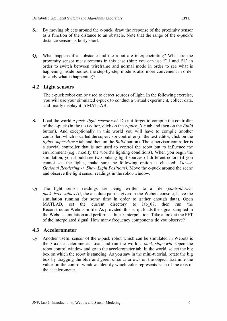
Valentino Braitenberg presented in his book “Vehicles: Experiments in Synthetic Psychology” (The MIT Press, 1984) several interesting ideas for developing simple, reactive control architectures and obtaining several different behaviors. In this lab, we want to see what we can achieve if e-pucks are programmed as Braitenberg vehicles. Figure 5 shows four different Braitenberg vehicles.

Figure 5: Four Braitenberg vehicles. Plus signs correspond to excitatory connections, minus signs to inhibitory ones. Vehicle 2a avoids light by accelerating away from it. Vehicle 2b exhibits a light approaching and following behavior, accelerating more and more as approaches the source. Vehicle 3a avoids light by braking and accelerating away toward darker areas. Finally, vehicle 3b approaches light but brakes and stops in front of it.

Q7: Which vehicle depicted in Figure 5 do you expect to be most effective at avoiding obstacles if light sensors were to be replaced by proximity sensors, and why?

In the remainder of this lab, we are going to tune the parameters of a Braitenberg controller on distance sensors (instead of light sensors) and exclusively using a linear perception-to-action map (i.e., essentially an 8x2 coefficient matrix, because we have 8 inputs and 2 outputs).

The principle of a Braitenberg controller is to directly compute the wheel speeds from the sensor values using a simple linear combination of parameters and sensor values:

speed!"#$ = α!"#$,!!

!!!(1−

ps_value!ps_range)

speed!"#$% = α!"#$%,!!

!!!(1−

ps_value!ps_range)

where ps_value! is the value of the i-th proximity sensor, ps_range is the acceptable range of sensor values, and α!"#$,! and α!"#$%,! are two design parameters.

The image cannot be displayed. Your computer may not have enough memory to open the image, or the image may have been corrupted. Restart your computer, and then open the file again. If the red x still appears, you may have to delete the image and then insert it again.

Distributed Intelligent Systems and Algorithms Laboratory EPFL

JNP, Lab 7: Introduction to Webots and Sensor Modeling 8

S8: Open the world e-puck_braitenberg.wbt, and look at the controller e-

puck_braitenberg.c. Observe the structure of the controller and identify the part of the code to be completed or modified. How does the code implement the Braitenberg controller described above?

Q9: What is the influence of the parameter, say, α!"#$,! on the speed of the left wheel? Hint: explain what happens if α!"#$,! is large or small when an obstacle is detected by the proximity sensor ps0 (recall Figure 4).

I10: Modify the parameters of the controller e-puck_braitenberg.c so that you achieve

these behaviors (see note in code): 1. The robot is moving forward while smoothly avoiding obstacles.

2. The robot is moving forward while being attracted by obstacles.

Remember to “Build” your controller after you make a change: Hint: To tune Braitenberg parameters, start with all coefficients at zero. Use only the two proximity sensors at the front, before completing the solution using all proximity sensors.

5.2 The role of noise in robotics simulations It is possible to configure the noise on sensor readings and motor outputs in the

Webots simulator in order to model what happens in the real world. Real-world noise can cause poor performance on many algorithms which perform very well theoretically. However, if treated correctly, noise can also be used to positive effect in some systems. In some cases, noise can even become an important ingredient of the algorithm. Hereafter, you will investigate the role of noise for escaping deadlocks in an obstacle avoidance situation.

S11: Open and run the e-puck_no_noise.wbt world; in this example the noise of all the

proximity sensors is set to 0 and the robot must avoid the V-shaped obstacle without remaining stuck. Run this simulation several times. Report the number of runs and the success rate of the robot.

Q12: What happens? Why?

S13: Now, open and run the e-puck_medium_noise.wbt world, which is exactly the same as e-puck_no_noise.wbt, except for the noise of the proximity sensors of the e-puck. Run this simulation as many times as the previous experiment without noise. Report the number of runs and the success rate of the robot. Discuss briefly the differences with the previous experiment without noise.

Distributed Intelligent Systems and Algorithms Laboratory EPFL

JNP, Lab 7: Introduction to Webots and Sensor Modeling 9

Q14: What is the noise on the proximity sensors of the e-puck in the e-puck_medium_noise.wbt world (hint, try to expand the model of the e-puck in the scene tree and look for the lookup table of the distance sensors)?

Consult the following Reference Manual page to find out how to interpret the proximity sensor lookup table: http://www.cyberbotics.com/reference/section3.23.php

S15: Now, open and run the e-puck_huge_noise.wbt world. Run this simulation as

many times as the previous experiment without noise. Report the number of runs and the success rate of the robot.

Q16: What happens now? What does it tell us about noise in robotics experiments?