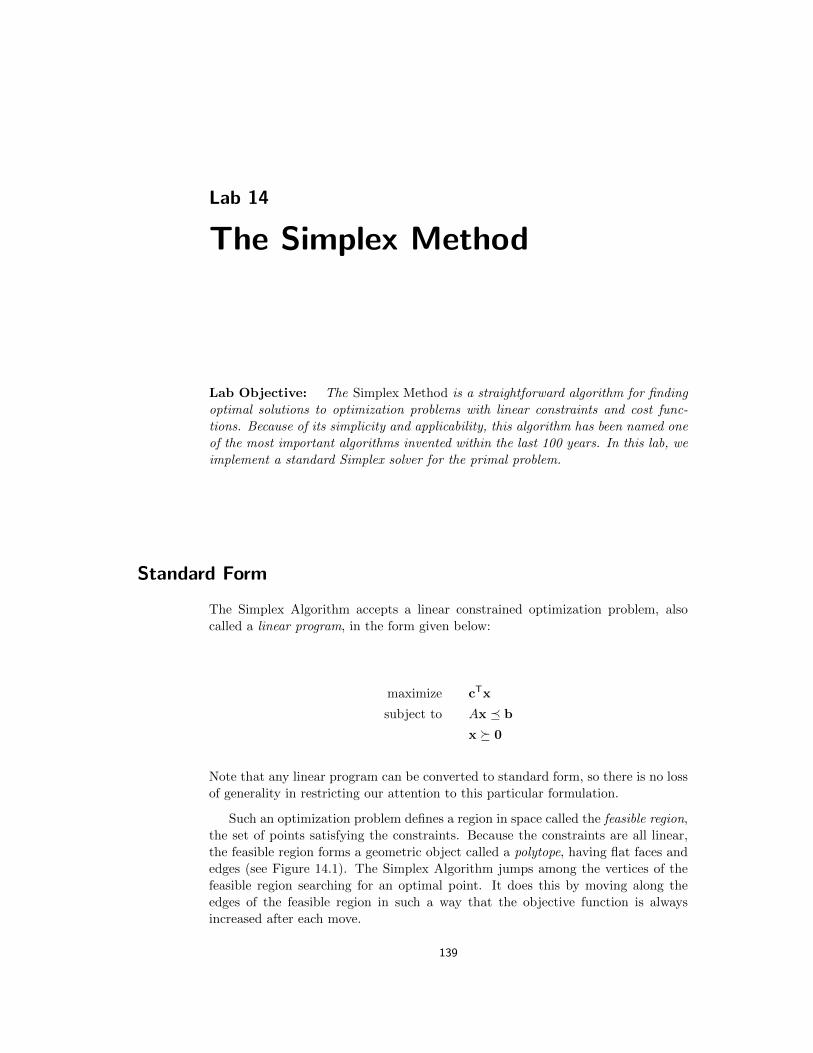
Lab 14

The Simplex Method

Lab Objective: The Simplex Method is a straightforward algorithm for findingoptimal solutions to optimization problems with linear constraints and cost func-tions. Because of its simplicity and applicability, this algorithm has been named oneof the most important algorithms invented within the last 100 years. In this lab, weimplement a standard Simplex solver for the primal problem.

Standard Form

The Simplex Algorithm accepts a linear constrained optimization problem, alsocalled a linear program, in the form given below:

maximize cTx

subject to Ax � b

x ⌫ 0

Note that any linear program can be converted to standard form, so there is no lossof generality in restricting our attention to this particular formulation.

Such an optimization problem defines a region in space called the feasible region,the set of points satisfying the constraints. Because the constraints are all linear,the feasible region forms a geometric object called a polytope, having flat faces andedges (see Figure 14.1). The Simplex Algorithm jumps among the vertices of thefeasible region searching for an optimal point. It does this by moving along theedges of the feasible region in such a way that the objective function is alwaysincreased after each move.

139

140 Lab 14. The Simplex Method

(a) The feasible region for a linear program

with 2-dimensional constraints.

x⇤

(b) The feasible region for a linear program

with 3-dimensional constraints.

Figure 14.1: If an optimal point exists, it is one of the vertices of the polyhedron.The simplex algorithm searches for optimal points by moving between adjacentvertices in a direction that increases the value of the objective function until it findsan optimal vertex.

Implementing the Simplex Algorithm is straightforward, provided one carefullyfollows the procedure. We will break the algorithm into several small steps, andwrite a function to perform each one. To become familiar with the execution of theSimplex algorithm, it is helpful to work several examples by hand.

The Simplex Solver

Our program will be more lengthy than many other lab exercises and will consist of acollection of functions working together to produce a final result. It is important toclearly define the task of each function and how all the functions will work together.If this program is written haphazardly, it will be much longer and more di�cult toread than it needs to be. We will walk you through the steps of implementing theSimplex Algorithm as a Python class.

For demonstration purposes, we will use the following linear program.

maximize 3x0

+ 2x1

subject to x0

� x1

2

3x0

+ x1

5

4x0

+ 3x1

7

x0

, x1

� 0.

Accepting a Linear Program

Our first task is to determine if we can even use the Simplex algorithm. Assumingthat the problem is presented to us in standard form, we need to check that thefeasible region includes the origin.

141

Problem 1. Write a class that accepts the arrays c, A, and b of a linearoptimization problem in standard form. In the constructor, check that thesystem is feasible at the origina. That is, check that Ax � b when x = 0.Raise a ValueError if the problem is not feasible at the origin.

aFor now, we only check for feasibility at the origin. A more robust solver sets up the

auxiliary problem and solves it to find a starting point if the origin is infeasible.

Adding Slack Variables

The next step is to convert the inequality constraints Ax � b into equality con-straints by introducing a slack variable for each constraint equation. If the con-straint matrix A is an m⇥ n matrix, then there are m slack variables, one for eachrow of A. Grouping all of the slack variables into a vector w of length m, theconstraints now take the form Ax+w = b. In our example, we have

w =

2

4

x2

x3

x4

3

5

When adding slack variables, it is useful to represent all of your variables, boththe original primal variables and the additional slack variables, in a convenientmanner. One e↵ective way is to refer to a variable by its subscript. For example,we can use the integers 0 through n�1 to refer to the original (non-slack) variablesx0

through xn�1

, and we can use the integers n through n+m�1 to track the slackvariables (where the slack variable corresponding to the ith row of the constraintmatrix is represented by the index n+ i� 1).

We also need some way to track which variables are basic (non-zero) and whichvariables are nonbasic (those that have value 0). A useful representation for thevariables is a Python list (or NumPy array), where the elements of the list areintegers. Since we know how many basic variables we have (m), we can partitionthe list so that all the basic variables are kept in the first m locations, and all thenon-basic variables are stored at the end of the list. The ordering of this list isimportant. In particular, if i m, the ith element of the list represents the basicvariable corresponding to the ith row of A. Henceforth we will refer to this list asthe index list.

Initially, the basic variables are simply the slack variables, and their valuescorrespond to the values of the vector b. In our example, we have 2 primal variablesx0

and x1

, and we must add 3 slack variables. Thus, we instantiate the followingindex list:

>>> L = [2, 3, 4, 0, 1]

Notice how the first 3 entries of the index list are 2, 3, 4, the indices representingthe slack variables. This reflects the fact that the basic variables at this point areexactly the slack variables.

142 Lab 14. The Simplex Method

As the Simplex Algorithm progresses, however, the basic variables change, andit will be necessary to swap elements in our index list. For example, suppose thevariable represented by the index 4 becomes nonbasic, while the variable representedby index 0 becomes basic. In this case we swap these two entries in the index list.

>>> L[2], L[3] = L[3], L[2]

>>> L

[2, 3, 0, 4, 1]

Now our index list tells us that the current basic variables have indices 2, 3, 0.

Problem 2. Design and implement a way to store and track all of the basicand non-basic variables.

Hint: Using integers that represent the index of each variable is usefulfor Problem 4.

Creating a Tableau

After we have determined that our program is feasible, we need to create the tableau(sometimes called the dictionary), a data structure to track the state of the algo-rithm. You may structure the tableau to suit your specific implementation. Re-member that your tableau will need to include in some way the slack variables thatyou created in Problem 2.

There are many di↵erent ways to build your tableau. One way is to mimic thetableau that is often used when performing the Simplex Algorithm by hand. Define

A =⇥

A Im

⇤

,

where Im

is the m⇥m identity matrix, and define

c =

c

0

�

.

That is, c 2 Rn+m such that the first n entries are c and the final m entries arezeros. Then the initial tableau has the form

T =

0 �cT 1b A 0

�

(14.1)

The columns of the tableau correspond to each of the variables (both primaland slack), and the rows of the tableau correspond to the basic variables. Using theconvention introduced above of representing the variables by indices in the indexlist, we have the following correspondence:

column i , index i� 2, i = 2, 3, . . . , n+m+ 1,

androw j , L

j�1

, j = 2, 3, . . . ,m+ 1,

143

where Lj�1

refers to the (j � 1)th entry of the index list.

For our example problem, the initial index list is

L = (2, 3, 4, 0, 1),

and the initial tableau is

T =

2

6

6

4

0 �3 �2 0 0 0 12 1 �1 1 0 0 05 3 1 0 1 0 07 4 3 0 0 1 0

3

7

7

5

.

The third column corresponds to index 1, and the fourth row corresponds to index4, since this is the third entry of the index list.

The advantage of using this kind of tableau is that it is easy to check the progressof your algorithm by hand. The disadvantage is that pivot operations require carefulbookkeeping to track the variables and constraints.

Problem 3. Add a method to your Simplex solver that will create the initialtableau as a NumPy array.

Pivoting

Pivoting is the mechanism that really makes Simplex useful. Pivoting refers to theact of swapping basic and nonbasic variables, and transforming the tableau appro-priately. This has the e↵ect of moving from one vertex of the feasible polytope toanother vertex in a way that increases the value of the objective function. Depend-ing on how you store your variables, you may need to modify a few di↵erent partsof your solver to reflect this swapping.

When initiating a pivot, you need to determine which variables will be swapped.In the tableau representation, you first find a specific element on which to pivot,and the row and column that contain the pivot element correspond to the variablesthat need to be swapped. Row operations are then performed on the tableau sothat the pivot column becomes an elementary vector.

Let’s break it down, starting with the pivot selection. We need to use somecare when choosing the pivot element. To find the pivot column, search from leftto right along the top row of the tableau (ignoring the first column), and stop onceyou encounter the first negative value. The index corresponding to this column willbe designated the entering index, since after the full pivot operation, it will enterthe basis and become a basic variable.

Using our initial tableau T in the example, we stop at the second column:

T =

2

6

6

4

0 �3 �2 0 0 0 12 1 �1 1 0 0 05 3 1 0 1 0 07 4 3 0 0 1 0

3

7

7

5

144 Lab 14. The Simplex Method

We now know that our pivot element will be found in the second column. Theentering index is thus 0.

Next, we select the pivot element from among the positive entries in the pivotcolumn (ignoring the entry in the first row). If all entries in the pivot column arenon-positive, the problem is unbounded and has no solution. In this case, the algo-rithm should terminate. Otherwise, assuming our pivot column is the jth columnof the tableau and that the positive entries of this column are T

i1,j , Ti2,j , . . . , Tik,j ,we calculate the ratios

Ti1,1

Ti1,j

,Ti2,1

Ti2,j

, . . . ,Tik,1

Tik,j

,

and we choose our pivot element to be one that minimizes this ratio. If multipleentries minimize the ratio, then we utilize Bland’s Rule, which instructs us to choosethe entry in the row corresponding to the smallest index (obeying this rule is impor-tant, as it prevents the possibility of the algorithm cycling back on itself infinitely).The index corresponding to the pivot row is designated as the leaving index, sinceafter the full pivot operation, it will leave the basis and become a nonbasic variable.

In our example, we see that all entries in the pivot column (ignoring the entryin the first row, of course) are positive, and hence they are all potential choices forthe pivot element. We then calculate the ratios, and obtain

2

1= 2,

5

3= 1.66...,

7

4= 1.75.

We see that the entry in the third row minimizes these ratios. Hence, the elementin the second column, third row is our designated pivot element, and our leavingindex is L

2

= 3:

T =

2

6

6

4

0 �3 �2 0 0 0 12 1 �1 1 0 0 05 3 1 0 1 0 07 4 3 0 0 1 0

3

7

7

5

Problem 4. Write a method that will determine the pivot row and pivotcolumn according to Bland’s Rule.

Definition 14.1 (Bland’s Rule). Choose the nonbasic variable with thesmallest index that has a positive coe�cient in the objective function as theleaving variable. Choose the basic variable with the smallest index among allthe binding basic variables.

Bland’s Rule is important in avoiding cycles when performing pivots.This rule guarantees that a feasible Simplex problem will terminate in afinite number of pivots.

The next step is to swap the entering and leaving indices in our index list. Inthe example, we determined above that these indices are 0 and 3. We swap these

145

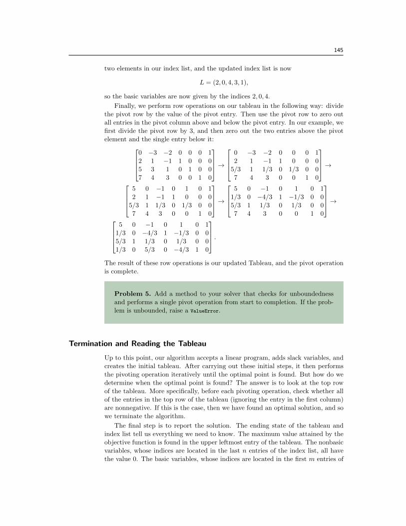
two elements in our index list, and the updated index list is now

L = (2, 0, 4, 3, 1),

so the basic variables are now given by the indices 2, 0, 4.

Finally, we perform row operations on our tableau in the following way: dividethe pivot row by the value of the pivot entry. Then use the pivot row to zero outall entries in the pivot column above and below the pivot entry. In our example, wefirst divide the pivot row by 3, and then zero out the two entries above the pivotelement and the single entry below it:

2

6

6

4

0 �3 �2 0 0 0 12 1 �1 1 0 0 05 3 1 0 1 0 07 4 3 0 0 1 0

3

7

7

5

!

2

6

6

4

0 �3 �2 0 0 0 12 1 �1 1 0 0 05/3 1 1/3 0 1/3 0 07 4 3 0 0 1 0

3

7

7

5

!

2

6

6

4

5 0 �1 0 1 0 12 1 �1 1 0 0 05/3 1 1/3 0 1/3 0 07 4 3 0 0 1 0

3

7

7

5

!

2

6

6

4

5 0 �1 0 1 0 11/3 0 �4/3 1 �1/3 0 05/3 1 1/3 0 1/3 0 07 4 3 0 0 1 0

3

7

7

5

!

2

6

6

4

5 0 �1 0 1 0 11/3 0 �4/3 1 �1/3 0 05/3 1 1/3 0 1/3 0 01/3 0 5/3 0 �4/3 1 0

3

7

7

5

.

The result of these row operations is our updated Tableau, and the pivot operationis complete.

Problem 5. Add a method to your solver that checks for unboundednessand performs a single pivot operation from start to completion. If the prob-lem is unbounded, raise a ValueError.

Termination and Reading the Tableau

Up to this point, our algorithm accepts a linear program, adds slack variables, andcreates the initial tableau. After carrying out these initial steps, it then performsthe pivoting operation iteratively until the optimal point is found. But how do wedetermine when the optimal point is found? The answer is to look at the top rowof the tableau. More specifically, before each pivoting operation, check whether allof the entries in the top row of the tableau (ignoring the entry in the first column)are nonnegative. If this is the case, then we have found an optimal solution, and sowe terminate the algorithm.

The final step is to report the solution. The ending state of the tableau andindex list tell us everything we need to know. The maximum value attained by theobjective function is found in the upper leftmost entry of the tableau. The nonbasicvariables, whose indices are located in the last n entries of the index list, all havethe value 0. The basic variables, whose indices are located in the first m entries of

146 Lab 14. The Simplex Method

the index list, have values given by the first column of the tableau. Specifically, thebasic variable whose index is located at the ith entry of the index list has the valueTi+1,1

.

In our example, suppose that our algorithm terminates with the tableau andindex list in the following state:

T =

2

6

6

4

5.2 0 0 0 .2 .6 1.6 0 0 1 �1.4 .8 01.6 1 0 0 .6 �.2 0.2 0 1 0 �.8 .6 0

3

7

7

5

L = (2, 0, 1, 3, 4).

Then the maximum value of the objective function is 5.2. The nonbasic variableshave indices 3, 4 and have the value 0. The basic variables have indices 2, 0, and 1,and have values .6, 1.6, and .2, respectively. In the notation of the original problemstatement, the solution is given by

x0

= 1.6

x1

= .2.

Problem 6. Write an additional method in your solver called solve() thatobtains the optimal solution, then returns the maximum value, the basic vari-ables, and the nonbasic variables. The basic and nonbasic variables shouldbe represented as two dictionaries that map the index of the variable to itscorresponding value.

For our example, we would return the tuple (5.2, {0: 1.6, 1: .2, 2: .6},

{3: 0, 4: 0}).

At this point, you should have a Simplex solver that is simple to use. Thefollowing code demonstrates how your solver is expected to behave:

>>> import SimplexSolver

# Initialize objective function and constraints.

>>> c = np.array([3., 2])

>>> b = np.array([2., 5, 7])

>>> A = np.array([[1., -1], [3, 1], [4, 3]])

# Instantiate the simplex solver, then solve the problem.

>>> solver = SimplexSolver(c, A, b)

>>> sol = solver.solve()

>>> print(sol)

(5.200,

{0: 1.600, 1: 0.200, 2: 0.600},

{3: 0, 4: 0})

If the linear program were infeasible at the origin or unbounded, we would expectthe solver to alert the user by raising an error.

147

Note that this simplex solver is not fully operational. It can’t handle the caseof infeasibility at the origin. This can be fixed by adding methods to your classthat solve the auxiliary problem, that of finding an initial feasible tableau whenthe problem is not feasible at the origin. Solving the auxiliary problem involvespivoting operations identical to those you have already implemented, so adding thisfunctionality is not overly di�cult.

The Product Mix Problem

We now use our Simplex implementation to solve the product mix problem, whichin its basic form can be expressed as a simple linear program. Suppose that amanufacturer makes n products using m di↵erent resources (labor, raw materials,machine time available, etc). The ith product is sold at a unit price p

i

, and thereare at most m

j

units of the jth resource available. Additionally, each unit of theith product requires a

j,i

units of resource j. Given that the demand for product iis d

i

units per a certain time period, how do we choose the optimal amount of eachproduct to manufacture in that time period so as to maximize revenue, while notexceeding the available resources?

Let x1

, x2

, . . . , xn

denote the amount of each product to be manufactured. Thesale of product i brings revenue in the amount of p

i

xi

. Therefore our objectivefunction, the profit, is given by

n

X

i=1

pi

xi

.

Additionally, the manufacture of product i requires aj,i

xi

units of resource j. Thuswe have the resource constraints

n

X

i=1

aj,i

xi

mj

for j = 1, 2, . . . ,m.

Finally, we have the demand constraints which tell us not to exceed the demandfor the products:

xi

di

for i = 1, 2, . . . , n

The variables xi

are constrained to be nonnegative, of course. We therefore havea linear program in the appropriate form that is feasible at the origin. It is a simpletask to solve the problem using our Simplex solver.

Problem 7. Solve the product mix problem for the data contained in thefile productMix.npz. In this problem, there are 4 products and 3 resources.The archive file, which you can load using the function np.load, contains adictionary of arrays. The array with key 'A' gives the resource coe�cientsai,j

(i.e. the (i, j)-th entry of the array give ai,j

). The array with key 'p'gives the unit prices p

i

. The array with key 'm' gives the available resourceunits m

j

. The array with key 'd' gives the demand constraints di

.

Report the number of units that should be produced for each product.

148 Lab 14. The Simplex Method

Beyond Simplex

The Computing in Science and Engineering journal listed Simplex as one of thetop ten algorithms of the twentieth century [Nash2000]. However, like any otheralgorithm, Simplex has its drawbacks.

In 1972, Victor Klee and George Minty Cube published a paper with severalexamples of worst-case polytopes for the Simplex algorithm [Klee1972]. In theirpaper, they give several examples of polytopes that the Simplex algorithm strugglesto solve.

Consider the following linear program from Klee and Minty.

max 2n�1x1

+2n�2x2

+ · · · +2xn�1

+xn

subject to x1

5

4x1

+x2

25

8x1

+4x2

+x3

125

......

2nx1

+2n�1x2

+ · · · +4xn�1

+xn

5

Klee and Minty show that for this example, the worst case scenario has ex-ponential time complexity. With only n constraints and n variables, the simplexalgorithm goes through 2n iterations. This is because there are 2n extreme points,and when starting at the point x = 0, the simplex algorithm goes through all of theextreme points before reaching the optimal point (0, 0, . . . , 0, 5n). Other algorithms,such as interior point methods, solve this problem much faster because they are notconstrained to follow the edges.