LA-UR- - Data science · LA-UR- Approved for public release; distribution is unlimited. Los Alamos...

Form 836 (7/06)

LA-UR- Approved for public release; distribution is unlimited.

Los Alamos National Laboratory, an affirmative action/equal opportunity employer, is operated by the Los Alamos National Security, LLC for the National Nuclear Security Administration of the U.S. Department of Energy under contract DE-AC52-06NA25396. By acceptance of this article, the publisher recognizes that the U.S. Government retains a nonexclusive, royalty-free license to publish or reproduce the published form of this contribution, or to allow others to do so, for U.S. Government purposes. Los Alamos National Laboratory requests that the publisher identify this article as work performed under the auspices of the U.S. Department of Energy. Los Alamos National Laboratory strongly supports academic freedom and a researcher’s right to publish; as an institution, however, the Laboratory does not endorse the viewpoint of a publication or guarantee its technical correctness.

Title:

Author(s):

Intended for:

LA-UR-07-1953

The Cosmic Code Comparison Project

Katrin Heitmann(1), Zarija Lukic(2), Patricia Fasel(1),Salman Habib(1), Michael S. Warren(1), Martin White(3),James Ahrens(1), Lee Ankeny(1), Ryan Armstrong(4), BrianO’Shea(1), Paul M. Ricker(2,5), Volker Springel(6), JoachimStadel(7), Hy Trac(8)

(1) Los Alamos National Laboratory, Los Alamos, NM 87545(2) University of Illinois, Dept. of Astronomy, Urbana, IL 61801(3) Dept. of Astronomy, University of California Berkeley, CA 94720-3411(4) UC Davis, Dept. of Computer Science, Davis, CA 95616(5) National Center for Supercomputing Applications, Urbana, IL 61801(6) Max-Planck-Institute for Astrophysics, 85741 Garching, Germany(7) University of Zurich, Inst. of Theoretical Physics, 8057 Zurich, Switzerland(8) Princeton University, Dept. of Astrophysical Sciences, NJ, 08544

E-mail: [email protected]

Abstract. Current and upcoming cosmological observations allow us to probestructures on smaller and smaller scales, entering highly nonlinear regimes.In order to obtain theoretical predictions in these regimes, large cosmologicalsimulations have to be carried out. The promised high accuracy from observationsmake the simulation task very demanding: the simulations have to be at least asaccurate as the observations. This requirement can only be fulfilled by carryingout an extensive code validation program. The first step of such a program is thecomparison of different cosmology codes including gravitation interactions only. Inthis paper we extend a recently carried out code comparison project to include fivemore simulation codes. We restrict our analysis to a small cosmological volumewhich allows us to investigate properties of halos. For the matter power spectrumand the mass function, the previous results hold, with the codes agreeing at the10% level over wide dynamic ranges. We extend our analysis to the comparisonof halo profiles and investigate the halo count as a function of local density.We introduce and discuss ParaView as a flexible analysis tool for cosmologicalsimulations, the use of which immensely simplifies the code comparison task.

arX

iv:0

706.

1270

v1 [

astr

o-ph

] 8

Jun

200

7

The Cosmic Code Comparison Project 2

1. Introduction

The last three decades have seen the emergence of cosmology as “precision science”,moving from order of magnitude estimates, to predictions and measurements ataccuracy levels better than 10%. Cosmic microwave background observations andlarge galaxy surveys have led this advance in the understanding of the origin andevolution of the Universe. Future surveys promise even higher accuracy, at the onepercent level, over a considerably wider dynamic range than probed earlier. In order tofully utilize the wealth of upcoming data and to address burning questions such as thedynamical nature of dark energy (specified by the equation of state parameter w = p/ρ,p being the pressure, and ρ the density), theoretical predictions must attain at leastthe same level of accuracy as the observations, even higher accuracy being certainlypreferable. The highly nonlinear physics at the length scales probed, combined withcomplicated gas physics and astrophysical feedback processes at these scales, makethis endeavor a daunting task.

As a first step towards achieving the final goal, a necessary requirement isto reach the desired accuracy for gravitational interactions alone, down to therelevant nonlinear scales. Tests with exact solutions such as pancake collapse [1] arevaluable for this task, but as shown in Ref. [2] the results do not easily translateinto statements about the accuracy of different simulation algorithms in realisticcosmological simulations. Exactly solvable problems are typically highly symmetricand hence somewhat artificial. Codes optimized for realistic situations can break downin certain tests even if their results appear to converge in physically relevant settings.Therefore, in order to evaluate the accuracy of simulation codes, a broad suite ofconvergence and direct code comparison tests must be carried out.

The codes used in this comparison project are all well-established, and have beenkey drivers in obtaining numerous scientific results. They are based on differentalgorithms and employ different methods for error control. The code developershave already carried out careful convergence tests themselves and verified to theirsatisfaction that the codes yield reliable results. But because of the multi-scalecomplexity of the dynamical problem itself, as well as the incompleteness of mostconvergence tests, it is necessary to do much more. Therefore, the aim here is tofocus on comparing results from a suite of different codes for realistic cosmologicalsimulations. In order to avoid uncertainties from statistical sampling, all codes arerun with exactly the same initial conditions, and all results are analyzed using thesame diagnostic tools.

The paper is organized as follows. In Section 2 we describe the ten simulationcodes used for the comparison study. In Section 3 we briefly describe the simulationscarried out for this project. Next, we introduce ParaView in Section 4, one of the mainanalysis tools used in this work. We present our results in Section 5 and conclude inSection 6.

2. The Codes

The ten codes used in this paper cover a variety of methods and application arenas.The simulation methods employed include parallel particle-in-cell (PIC) techniques(the PM codes MC2 and PMM, the PM/AMR codes Enzo and FLASH), a hybridof PIC and direct N-body (the AP3M code Hydra), tree algorithms (the treecodesPKDGRAV and HOT), and hybrid tree-PM algorithms (GADGET-2, TPM, and


TreePM).The PIC method models many-body evolution problems by solving the equations

of motion of a set of tracer particles which represent a sampling of the system phasespace distribution function. A computational grid is used to increase the efficiencyof the self-consistent inter-particle force calculation. To increase dynamic range, localforce computations (e.g., P3M, tree-PM) and AMR are often used. The grid alsoprovides a natural basis for coupling to hydro-solvers.

Treecodes are based on the idea that the gravitational potential of a far-awaygroup of particles is accurately given by a low-order multipole expansion. Particlesare first arranged in a hierarchical system of groups in a tree structure. Computingthe potential at a point turns into a descent through the tree. Treecodes naturallyembody an adaptive force resolution scheme without the overhead of a computationalgrid. Tree-PM is a hybrid algorithm that combines a long-range force computationusing a grid-based technique, with shorter-range force computation handled by a treealgorithm. In the following we give a brief description of each code used in thiscomparison study.

2.1. The Grid Codes

2.1.1. MC2 The multi-species Mesh-based Cosmology Code MC2 code suite includesa parallel PM solver for application to large scale structure formation problems incosmology. In part, the code descended from parallel space-charge solvers for studyinghigh-current charged-particle beams developed at Los Alamos National Laboratoryunder a DOE Grand Challenge [3, 4]. MC2 solves the Vlasov-Poisson systemof equations for an expanding universe using standard mass deposition and forceinterpolation methods allowing for periodic or open boundary conditions with secondand fourth-order (global) symplectic time-stepping and a Fast Fourier Transform(FFT)-based Poisson solver. The results reported in this paper were obtained usingCloud-In-Cell (CIC) deposition/interpolation. The overall computational scheme hasproven to be remarkably accurate and efficient: relatively large time-steps are possiblewith exceptional energy conservation being achieved.

2.1.2. PMM Particle-Multi-Mesh (PMM) [5] is an improved PM algorithmthat combines high mass resolution with moderate spatial resolution while beingcomputationally fast and memory friendly. The current version utilizes a two-levelmesh FFT-based gravity solver where the gravitational forces are separated into long-range and short-range components. The long-range force is computed on the root-level, global mesh, much like in a PM code. To obtain higher spatial resolution, thedomain is decomposed into cubical regions and the short-range force is computed ona refinement-level, local mesh. This algorithm achieves a spatial resolution of 4 timesbetter than a standard one-level mesh PM code at the same cost in memory. In [5],PMM is shown to achieve very similar accuracy to that of MC2 when run with thesame minimum grid spacing.

2.1.3. Enzo Enzo‡ is a publicly available, extensively tested adaptive meshrefinement (AMR), grid-based hybrid code (hydro + N-Body) which was originallywritten by Greg Bryan, and is now maintained by the Laboratory for Computational

‡ http://lca.ucsd.edu/codes/currentcodes/enzo


Astrophysics at UC San Diego [6, 7, 8, 9]. The code was originally designed to dosimulations of cosmological structure formation, but has been modified to examineturbulence, galactic star formation, and other topics of interest. Enzo uses the Berger& Colella method of block-structured adaptive mesh refinement [10]. It couples anadaptive particle-mesh method for solving the equations of dark matter dynamics[11, 12] with a hydro solver using the piecewise parabolic method (PPM), which hasbeen modified for cold, hypersonic astrophysical flows by the addition of a dual-energyformalism [13, 14]. In addition, the code has physics packages for radiative cooling,a metagalactic ultraviolet background, star formation and feedback, primordial gaschemistry, and turbulent driving.

2.1.4. FLASH FLASH [15] originated as an AMR hydrodynamics code designed tostudy X-ray bursts, novae, and Type Ia supernovae as part of the DOE ASCI AlliancesProgram. Block-structured adaptive mesh refinement is provided via the PARAMESHlibrary [16]. FLASH uses an oct-tree refinement scheme similar to [17] and [18]. Eachmesh block contains the same number of zones (163 for the runs in this paper), and itsneighbors must be at the same level of refinement or one level higher or lower (meshconsistency criterion). Adjacent refinement levels are separated by a factor of two inspatial resolution. The refinement criterion used is based upon logarithmic densitythresholds. Numerous extensions to FLASH have been developed, including solversfor thermal conduction, magnetohydrodynamics, radiative cooling, self-gravity, andparticle dynamics. In particular, FLASH now includes a multigrid solver for self-gravity and an adaptive particle-mesh solver for particle dynamics. Together withthe PPM hydrodynamics module, these provide the core of FLASH’s cosmologicalsimulation capabilities. FLASH uses a variable time step leapfrog integrator. Inaddition to other time step limiters, the FLASH particle module requires that particlestravel no more than a fraction of a zone during a time step.

2.2. The Tree Codes

2.2.1. HOT This parallel tree code [19] has been evolving for over a decade on manyplatforms. The basic algorithm may be divided into several stages (the method of errortolerance is described in Ref. [20]). First, particles are domain decomposed into spatialgroups. Second, a distributed tree data structure is constructed. In the main stageof the algorithm, this tree is traversed independently in each processor, with requestsfor nonlocal data being generated as needed. A Key is assigned to each particle,which is based on Morton ordering. This maps the points in 3-dimensional space toa 1-dimensional list, maintaining as much spatial locality as possible. The domaindecomposition is obtained by splitting this list into Np (number of processors) pieces.An efficient mechanism for latency-hiding in the tree traversal phase of the algorithmis critical. To avoid stalls during nonlocal data access, effectively explicit ‘contextswitching’ is done using a software queue to keep track of which computations havebeen put aside waiting for messages to arrive. This code architecture allows HOT toperform efficiently on parallel machines with fairly high communication latencies [21].HOT has a global time stepping scheme. The code was among the ones used forthe original Santa Barbara Cluster Comparison Project [22] and also supports gasdynamics simulations via a smoothed particle hydrodynamics (SPH) module [23].


2.2.2. PKDGRAV The central data structure in PKDGRAV [24] is a tree structurewhich forms the hierarchical representation of the mass distribution. Unlike the moretraditional oct-tree which is used in the Barnes-Hut algorithm [25] and is implementedin HOT, PKDGRAV uses a k-D tree, which is a binary tree. The root-cell of this treerepresents the entire simulation volume. Other cells represent rectangular sub-volumesthat contain the mass, center-of-mass, and moments up to hexadecapole order oftheir enclosed regions. PKDGRAV calculates the gravitational accelerations using thewell known tree-walking procedure of the Barnes-Hut algorithm. Periodic boundaryconditions are implemented via the Ewald summation technique [26]. PKDGRAVuses adaptive time stepping. It runs efficiently on very large parallel computers andhas produced some of the world’s highest resolution simulations of cosmic structures.A hydrodynamics extension called GASOLINE exists.

2.3. The Hybrid Codes

2.3.1. Hydra HYDRA [27] is an adaptive P3M (AP3M) code with additional SPHcapability. In this paper we use HYDRA only in the collisionless mode by switchingoff gas dynamics. The P3M method combines mesh force calculations with directsummation of inter-particle forces on scales of two to three grid spacings. In regionsof strong clustering, the direct force calculations can become significantly expensive.In AP3M, this problem is tackled by utilizing multiple levels of subgrids in these highdensity regions, with direct force computations carried out on two to three spacingsof the higher-resolution meshes. Two different boundary conditions are implementedin HYDRA, periodic and isolated. The time step algorithm in the dark matter-onlymode is equivalent to a leapfrog algorithm.

2.3.2. GADGET-2 The N-body/SPH code GADGET-2 [28, 29] employs a tree method[25], to calculate gravitational forces. Optionally, the code uses a tree-PM algorithmbased on an explicit split in Fourier space between long-range and short-range forces[30]. This combination provides high performance while still retaining the full spatialadaptivity of the tree algorithm, allowing the code to reach high spatial resolutionthroughout a large volume. By default, GADGET-2 expands the tree multipoles onlyto monopole order, in favor of a compact tree storage, a cache-optimized tree-walk,and consistent and efficient dynamic tree updates. The cell-opening criterion used inthe tree walk is based on an estimator for the relative force error introduced by agiven particle-cell interaction, such that the tree force is accurate up to a prescribedmaximum relative force error. The latter can be lowered arbitrarily, if desired, atthe expense of higher calculation times. The PM part of GADGET-2 solves Poisson’sequation on a mesh with standard fast Fourier transforms, based on a CIC massassignment and a four-point finite differencing scheme to compute the gravitationalforces from the potential. The smoothing effects of grid assignment and interpolationare corrected by an appropriate deconvolution in Fourier space. The time-stepping ofGADGET-2 uses a leap-frog integrator which is symplectic in case constant timesteps(in the log of the expansion factor) are employed for all particles. However, thecode is normally run in a mode where individual and adaptive timesteps are usedto speed up the calculation time. To this end, the timesteps for the short-rangedynamics are allowed to freely adapt to any power of two subdivision of the long-range timestep. GADGET-2 is fully parallelized for massively parallel computers withdistributed memory, based on the MPI standard. The code can also be used to simulate


hydrodynamical processes using the particle-based smoothed particles hydrodynamics(SPH) method (e.g. [31]), in an entropy conserving formulation [32], a feature whichis however not exercised in the simulations considered in this paper.

2.3.3. TPM TPM [33, 34] is a publicly-available hybrid code combining a PMand a tree algorithm. The density field is broken down into many isolated high-density regions using a density threshold criterion. These contain most of the massin the simulation but only a small fraction of the volume. In these regions, thegravitational forces are computed with the tree algorithm while for the bulk of thevolume the forces are calculated via a PM algorithm, the PM time steps being largecompared to the time-steps for the tree-algorithm. The PM algorithm uses the CICdeposition/interpolation scheme and solves the Poisson equation using FFTs.The timeintegrator in TPM is a standard leap-frog scheme: the PM time steps are fixed whereastree particles have individual time steps, half of the PM step or smaller.

2.3.4. TreePM The algorithmic structure of the TreePM code [35] is very similarto GADGET-2. The particles are integrated using a second-order leap-frog method,with position and canonical momentum as the variables. The time step is dynamicallychosen as a small fraction (depending on the smoothing length) of the local free-falltime and particles have individual time steps. The force on any given particle iscomputed in two stages. The long-range component of the force is computed usingthe PM method, while the short range component is computed from a global tree. Aspline softened force law is used. The tree expands forces to monopole order only, andcells are opened based upon the more conservative of a geometric and relative forceerror criterion. The PM force is computed by direct FFT of the density grid obtainedfrom CIC mass assignment.

3. The Simulations

A previous code comparison suite [2] considered three cosmological test problems:the Santa Barbara Cluster [22], and two large-scale structure simulations of ΛCDMmodels in a 64h−1Mpc box and a 256h−1Mpc box. In the latter two cases, the primarytarget of this previous work was to investigate results in a medium resolution regime,addressing statistical quantities such as the two-point correlation function, the densityfluctuation power spectrum, and the dark matter halo mass function.

In this paper we focus further attention on one of these tests, the smaller of theΛCDM boxes. Due to the small box size, the force resolution of all codes – includingthe pure mesh codes – is in principle sufficient to analyze properties of individual halosthemselves. This allows us to extend the dynamic range of the code comparison tohigher resolution than studied earlier. In this new regime, we expect to see a muchbroader divergence of results because of the more demanding nature of the test. (Evenin the previous analysis [2], the power spectrum was unexpectedly deviant at the largerwavenumbers considered.) Our aim is to characterize the discrepancies and attemptto understand the underlying causes.

All codes were given exactly the same particle initial conditions at a redshiftzin = 50. The initial linear power spectrum was generated using a fit to the transferfunction [36], a modification of the BBKS fit [37]. This fit does not capture baryonoscillations but takes baryonic suppression into account (these details are of only


Table 1. Softening lengths measured in h−1kpc. The different smoothing kernelshave been converted into Plummer softening equivalents by matching the potentialat the origin. While this procedure is only approximate, it makes a comparisonof the different force resolutions more meaningful. For details on the conversionsee the main text.

MC2 PMM Enzo FLASH HOT PKDGRAV Hydra GADGET-2 TPM TreePM

62.5 62.5 62.5 62.5 7.1 1.6 28.4 7.1 5.1 5.7

limited relevance for the test). The cosmology underlying the simulations is given byΩCDM = 0.27, Ωb = 0.044, ΩΛ = 0.686, h = 0.71, σ8 = 0.84, and n = 0.99. Thesimulation was run with 2563 particles, which leads to an individual particle mass ofmp=1.362·109h−1M.

While performing a comprehensive code comparison study which involves verydifferent algorithms – such as grid and particle-based methods in the present case – acentral and difficult question immediately arises: what is the most informative way tocompare the codes and learn from the results? The difficulty is compounded by thefact that codes are often optimized under different criteria and controlling numericalerror is a complex multi-parameter problem in any case, even for codes that share thesame general underlying algorithm.

As a case in point, let us consider the choice of force resolution for each code.(Since the volume and number of particles are fixed, the mass resolution is the samefor each run.) One option would be to run all codes with the same formal forceresolution but this, aside from wasting resolution for the high-resolution codes, alsosuffers from the problem that it is not easy to compare resolutions across differentalgorithms; moreover, time-stepping errors also must be folded into these sorts ofestimates. Finally, such a comparison would be rather uninteresting, because realisticcosmological simulations are run with higher resolutions than would be possible in aconservative test of this type: Interesting effects on small scales would be missed. Amore uncontrolled, but nevertheless useful option is to allow every simulator to run heror his code with close to the optimal settings they would also use for a scientific run(given the other restrictions imposed by the test problem). In this case, a more realisticcomparison can be performed in which we can access the robustness of conclusionsfrom cosmological simulations. Here, while our approach adheres more closely to thesecond strategy, we do try to assess at what length scales one should expect a specificcode to break down assuming that the resolution of the code is accurately estimatedby the simulator.

The nominal resolutions for the different codes for the performed runs are as givenin Table 1. We have converted the different softening kernels into Plummer equivalentsfollowing the normalization conventions of Ref. [38]. We have matched the differentsoftening kernels φ at zero and compared them at this point. With the normalizationconventions in Ref. [38], we find:

φPlummer(0) ∝ 1ε, (1)

φSpline(0) ∝ 75

1ε, (2)

φK3(0) ∝ 2079512

1ε, (3)


where ε is the softening length. The grid resolution of the PM and AMR codes isroughly equivalent to the Plummer softening. HOT and Hydra have Plummer forcekernels implemented, PKDGRAV uses Dehnen’s K3 kernel [38] and the three tree-pmcodes use spline kernels. With the above definitions, it is easy to convert the splineand K3 kernels into Plummer via

εSpline = 1.4εPlummer, (4)εK3 = 4.06εPlummer, (5)

which we used to standardize the force resolution quotes in Table 1. We note thatsome of the codes below could have been run at higher resolution, and the valuesbelow should not be thought of as resolution limits. In fact, the choices of these valuesrepresent compromises due to run time considerations as well as a (loosely) pre-plannedscatter to try and determine the effects of force resolution on the simulation results.

4. Analysis Framework and Tools

Broadly speaking, the major aim of our code comparison project is to characterizedifferences in results from large cosmological simulation codes, identify the causesunderlying these differences, and, if possible, develop strategies to reduce or eliminatethe differences in order to obtain reliable results over large length and mass scales.If it is not possible to eliminate some of the differences, e.g. due to insufficient forceresolution in grid codes, it is still important to provide robust criteria that correctlydetermine the scales at which the code can be trusted, and with what accuracy.

The identification and characterization of differences in code results is not asstraightforward as it first appears. Certainly we may, and do, compare standardstatistical quantities such as low-order correlation functions. However, there is muchmore information in the data beyond this, e.g., large-scale structure morphology,substructure in the density field, and subtle features such as the variation in halobias as a function of the local environment. For these reasons, it is often very useful tosimply look at the region or object of interest in the simulation and compare it acrossthe different codes. Following this qualitative comparison – perhaps even inspired byit – the aim is to construct a hypothesis about the cause for the perceived differencewhich then has to be carefully tested with quantitative measures.

It is very desirable to have a framework which combines these two steps in aconvenient, and eventually seamless, manner. The framework should allow differencesand anomalies picked up by eye from data sets to be immediately queried andquantified using a programmable toolkit. An example relevant to cosmologicalsimulations is the following. Suppose we “see” fewer halos in one simulation comparedto another. The analysis tool should then provide quantitative information of thefollowing type: in what areas is the difference larger, what is the exact number countof the halos in this region, what is the difference in the environment (e.g. by comparingthe local density in the two codes), what is the halo history in the region, and so on.

As part of this paper we include an introduction of ParaView [39] § to thecosmology and the wider computational communities. ParaView has some of thefeatures discussed above built in and allows the user to implement additional analysistools. ParaView is an open-source, scalable visualization tool which is designed as a

§ We use ParaView 2.6 throughout this paper. This is the latest stable release which can bedownloaded at http://www.paraview.org/HTML/Download.html

http://www.paraview.org/HTML/Download.html


Figure 1. Screenshot of the comparative visualization manager in ParaView.Upper row: results from four different codes, zoomed into a dense region of thesimulations. Particles are displayed as arrow glyphs, colored with respect to theirvelocity magnitude. Lower row: same region, the particles now displayed simplyas dots.

layered architecture. The foundation and first layer of ParaView is the visualizationtoolkit (VTK). VTK provides data representations, algorithms, and a mechanism tointerconnect these to form a working program. The second layer is a parallel extensionto the visualization toolkit which supports streaming of all data types and parallelexecution on shared and distributed memory machines. The third layer is ParaViewitself. ParaView provides a graphical user interface and transparently supports thevisualization and rendering of large datasets via hardware acceleration, parallelism,and level-of-detail techniques.

For the code comparison project we have implemented a particle reader whichworks with the data format used throughout this paper. This allows other simulatorswho wish to test their codes against our results to use exactly the same analysis tool.As explained later, we have also implemented a diverse set of diagnostic tools relevantfor cosmological simulations. These help to ease the analysis of large simulation datasets and make it more efficient. We plan to extend the set of available analysis featuresin the near future.

5. Results

5.1. Results for the Full Simulation Box

As an initial test, a simple view of the simulation output at z = 0 proves to be veryuseful. ParaView offers a comparative visualization option in which the results fromdifferent simulations can be shown simultaneously. Manipulation on any one outputin this mode results in the same manipulation for all the others. ParaView allows


Figure 2. A subset of the 20,000 particles at z = 0 from the GADGET-2simulation (left) and the Enzo simulation (right). The particles are shown withvector arrow glyphs which are sized and colored by their velocity magnitude (blue:slowest, red: fastest).

fly-ins, rotation of the box, projections, and has many more features which make itconvenient to inspect the outcome of the simulation. A screenshot of the comparativevisualization manager is displayed in Figure 1 – a zoom into an arbitrary region of thesimulation box showing simultaneous results from four different codes. In the upperrow a subset of the particles is shown as arrow glyphs, colored by velocity magnitude,the lower row shows the particles as dots with the same coloring scheme. A quickinspection of these snapshots reveals that the code 2 run had a problem with thevelocities and code 4 had slightly incorrect boundary conditions (the whole picturebeing shifted upward). (Of course these initial bugs were fixed before going on to thefinal results discussed below!)

Figure 2 shows a comparison of the final GADGET-2 and Enzo outputs. We showa subsample of 20,000 particles, each displayed with vector arrow glyphs, sized andcolored by their velocity magnitude. The arrow glyphs nicely represent the flows inthe box to the major mass concentrations. As to be expected, particles in the fieldare slow (blue), while the particles in the halos have the largest velocities (yellow tored). While the overall appearance of both simulations shown is very similar, subtledifferences can be seen (e.g., there are no small structures in the flow regions in theEnzo simulations), indicating the higher resolution employed in the GADGET-2 run.(Five of the biggest halos in the simulation will be examined in more detail below, theresolution differences becoming significantly more apparent.)

5.2. Dark Matter Halos

The halo paradigm is central to any large-scale structure analysis; dark matter insimulations, discretized in the form of heavy collisionless particles, forms clearlyvisible filaments (stripes) and halos (clumps of dark matter) through the process ofgravitational instability. Figure 2 shows these structures clearly for the simulations


studied in this paper. This picture agrees well with observations of galaxy rotationcurves, and velocity dispersions of galaxies in clusters which favor scenarios whereluminous, baryonic matter is embedded in massive, extended, and close to sphericalconglomerates of dark matter. In simulations, dark matter halos can be identified and“weighed” in different ways. We can measure overdensities (see e.g. [40]) or use groupfinding algorithms such as friend-of-friend (FOF) algorithms [41] to find halos.

A remarkable feature of halos was found by Navarro, Frenk, and White [42]: darkmatter halos of all masses, from dwarf galaxies to the largest clusters of galaxies, havespherically-averaged density profiles that are well-described by a single, “universal”formula

ρ(r) =ρcδc

r/rs (1 + r/rs)2 . (6)

The scaling radius, rs, and characteristic overdensity, δc, are free parameters of themodel, while ρc is the critical density for closure of the Universe. Even though atheoretical explanation for this universal profile has not been found, the nature ofthe profile itself has received extensive support from simulations carried out by manydifferent groups [43] (there do remain questions about the behavior at very small radii,but these are not relevant here).

Here we are interested in the variation of the profiles produced by the differentcodes, tending towards the outer region of the halo. This variation may be significantfor determining halo masses via the often used FOF algorithm. The mass that thehalo finder will “see”, strongly depends on the density and density gradient close tothe virial radius (R200) of a halo. On the other hand, accurately reproducing theinner slope of a halo profile is the prime test of the code’s force resolution. On scalesbelow this resolution limit, particle positions get randomized, resulting in a flatteneddensity profile (numerical errors can also lead to a sharpening of the profile due to anassociated unphysical damping).

We first compare the five heaviest halos from the simulations; their masses rangebetween approximately 2 to 5 · 1014h−1M, thus each halo is sampled with 150,000or more particles. The individual halo masses (as found by the FOF algorithm) arein agreement within 3% for all ten codes. Note that the FOF masses found for thegrid codes are slightly higher. This is presumably due to their lower resolution inthis comparison, resulting in less tight halos. The FOF halo finder can identify moreparticles in the fuzzier outskirts of lower resolution simulations as belonging to thehalo than in the high resolution runs. The centers of the halos are defined by theminimum of the local potential of the halo. Here the agreement among the codes iseven better than for the masses – the difference is less than 0.5% of the box size. InTable 2 we show the center and mass of one of the halos, Halo 3. This halo (alsoshown in Figure 7) has the size and mass of a group of galaxies. The dispersion inthe mass and position of the center is similar for the other halos, whose profiles weinvestigate next.

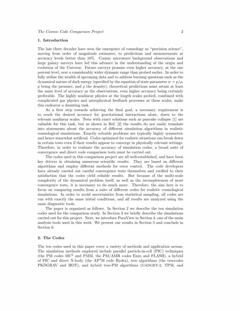
In Figure 3 we present the spherically averaged density profiles for the five heaviesthalos in the simulation. As an arbitrary reference, the black line represents the bestNFW fit (Equation 6) for the TPM data. The fit is shown up to the inner 10 h−1kpcof each halo. In addition, we show two residual panels for each halo profile. The upperpanel shows the ratio of all codes with respect to GADGET-2, while the lower panelshows only the four grid codes and ratios with respect to MC2.


Figure 3. Halo profiles for the five heaviest halos in the simulation. The black lineshows the best-fit NFW profile to the TPM simulation, mainly to guide the eye. In theouter regions all codes agree very well. In the inner regions the fall-off of the grid codesis as expected due to resolution limitations. The fall-off point can be predicted from thefinite force resolution and agrees well with the results. The middle panel in each plotshows the ratio of the different codes with respect to GADGET-2. The lower panelsshow only the four grid codes and the ratio with respect to MC2.


Table 2. Halo 3 data: distance of the center from the mean value for all codes,and the mass of the halo from different simulations.

Code ∆Xc [kpc/h] ∆Yc [kpc/h] ∆Zc [kpc/h] Mass [1014 M/h]

MC2 -86.23 158.81 -14.68 2.749

PMM 201.68 33.90 10.24 2.757

Enzo -21.36 45.16 11.36 2.745

FLASH -41.66 -22.56 -23.10 2.726

HOT -30.02 -120.54 43.99 2.720

PKDGRAV 38.58 52.19 -43.98 2.679

Hydra 19.91 -28.29 0.77 2.721

GADGET-2 -27.08 -59.00 -0.70 2.705

TPM -36.37 -35.09 1.04 2.697

TreePM -17.45 -24.62 13.63 2.727

The agreement in the outer part of the halos is excellent. As expected, the codesexhibit different behaviors on small scales (depending on their force resolution andtime-stepping), thus the inner parts of halos are not always the same. While the highresolution codes successfully track the profile all the way in to the plotting limits ofFigure 3, the profiles from the mesh codes depart much earlier (60-100 h−1kpc), withapproximately constant density in the core. The onset of the flattening is consistentwith the nominal resolution of the grid codes, which is given in Table. 1. Note thatamong the mesh codes there is no significant difference between the fixed mesh codeswhich ran at the highest resolution throughout the whole simulation volume, and theAMR codes whose base mesh spacing is a factor of 4 times lower.

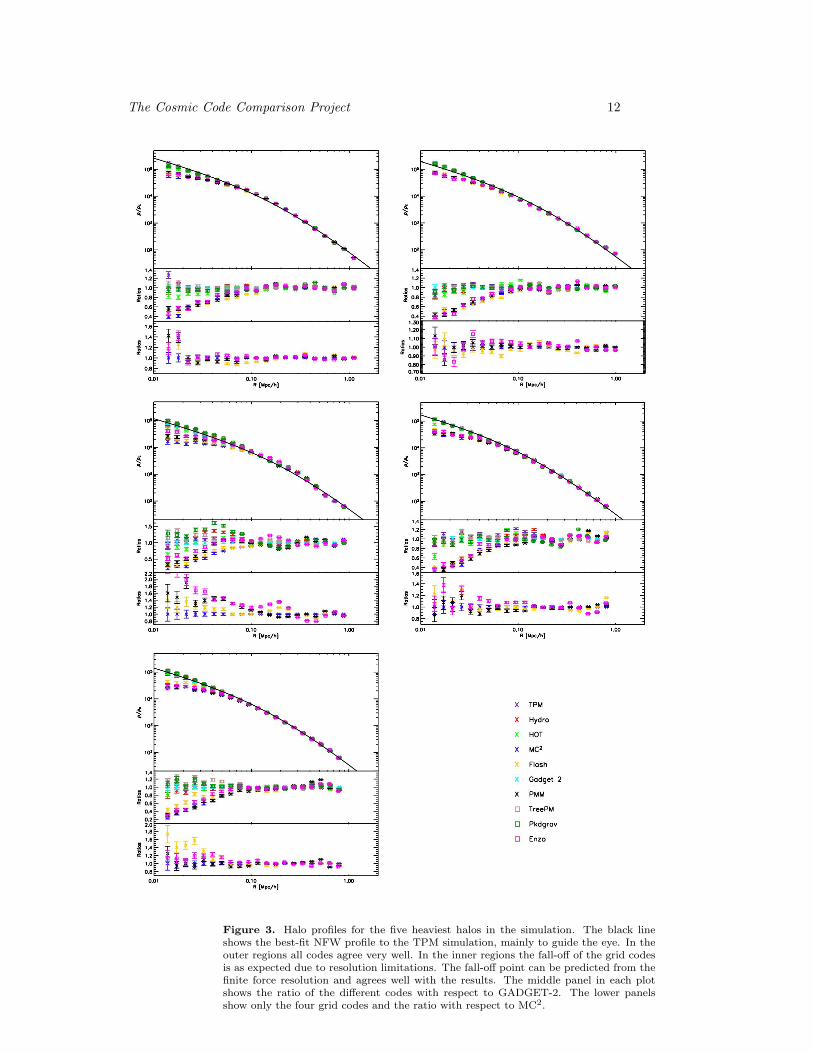
We now study three of the five halos in more detail, restricting attention toparticles within a sphere of radius 2 · R200. The profiles of the largest halo, Halo 1,shown in Figure 3, agree well down to R = 0.06h−1Mpc; at smaller scales the finiteresolution of the grid codes becomes apparent. Nevertheless, the grid codes and thehigh-resolution codes among themselves yield very consistent results. Figure 4 showsthe density of Halo 1 for the lower resolution code PMM and the higher resolution codeTreePM in two-dimensional projection. The two-dimensional density field is computedon a 100×100 grid within the 2 ·R200 region, projected onto the z-direction (anotherprojection along the x-direction is also shown). The projected density field has beennormalized by dividing out the mean density in this area. The mean density is veryclose across the different codes, hence the normalization allows for direct comparisonsof the projected density fields. As mentioned earlier, the positions of the halo centers(density peaks) are in remarkably good agreement. Due to its higher resolution, thedensity in the center of the halo from the TreePM run is slightly higher (as to beexpected from the profiles). In addition, TreePM shows slightly more substructureon the outskirts of the halo, displayed by the small “hills”. Overall, the halo is verysmooth and well defined, which is reflected in the good agreement of the profiles. Thedensity plots for the four grid codes are very similar. The small structures aroundthe halo in the other codes also show only very minor variations, thus the PMM andTreePM results can be considered to be representative.


Figure 4. Projected and normalized two-dimensional density for Halo1 from PMM (left) and TreePM (right). TreePM has a slightly higherdensity in the inner region of the halo than PMM, as to be expected fromthe different force resolutions. Overall the agreement is very good.

The profiles of Halo 3 show substantially more variation among the different codesin the inner region, relative to the other four halos. Studying it in more detail, wefirst investigate a subset of four codes: MC2, FLASH, GADGET-2, and HOT, coveringa wide range of force resolutions. In Figure 5 we show a zoom into the center of thehalo. The particles are shown in white. Superimposed on the particle distributionis a 2-dimensional density contour evaluated on a 100×100 grid and smoothed witha Gaussian filter, projected along the z-direction. (The contouring and filtering areintrinsic functions in ParaView.‖)

The overall appearance of the halo is remarkably similar between the codes,a major feature of the halo being its irregular shape. The left side of the halo iselongated and a second major peak has developed on the right, leading o a triangularshape in this projection. This irregularity (seen also very clearly in Figure 6) is mostlikely the reason for the disagreement in the inner part of the profiles. The halo hasprobably undergone a recent merger or is in the process of merging. Comparing thelower resolution runs from MC2 and FLASH with GADGET-2 and HOT, the effect offorce resolution is very apparent, the high resolution runs producing significantly moresubstructure. GADGET-2 shows slightly more substructure than HOT, which couldbe due to the adaptive time stepping used in the GADGET-2 run relative to HOT’sglobal time-step.

‖ ParaView provides a Gaussian filter called vtkGaussianSplatter. This is a filter that injects inputpoints into a structured points (volume) dataset. As each point is injected, it “splats” or distributesvalues to nearby voxels. Data is distributed using an elliptical, Gaussian distribution function.The distribution function is modified using scalar values (expands distribution) or normals (createsellipsoidal distribution rather than spherical). In general, the Gaussian distribution function f(x)around a given splat point p is given by f(x) = ScaleFactor·exp(ExponentFactor((r/Radius)2)) wherex is the current voxel sample point; r is the distance |x− p|, ExponentFactor ≤ 0.0, and ScaleFactorcan be multiplied by the scalar value of the point p that is currently being splatted. If points normalsare present (and NormalWarping is on), then the splat function becomes elliptical (as comparedto the spherical one described by the previous equation). The Gaussian distribution function thenbecomes: f(x) = ScaleFactor∗exp(ExponentFactor∗(((rxy/E)2 +z2)/R2)) where E is a user-definedeccentricity factor that controls the elliptical shape of the splat; z is the distance of the current voxelsample point along normal N ; and rxy is the distance of x in the direction perpendicular to N . Thisclass is typically used to convert point-valued distributions into a volume representation. The volumeis then usually iso-surfaced or volume rendered to generate a visualization. It can be used to createsurfaces from point distributions, or to create structure (i.e., topology) when none exists.


Figure 5. Two-dimensional contour plot of the projected density for Halo 3 fromMC2, FLASH, GADGET-2, and HOT (left upper to right lower plot). White:particles, black: contour smoothed with a Gaussian Filter.

Figure 6. Same as in Figure 5: MC2, FLASH, GADGET-2, and HOT.


48.8 49 49.2 49.4 49.6 49.8 50 50.2 50.4 59

59.5

60

60.5

61

0

10

20

30

40

50

60

70

PMM: Halo 3

48.8 49 49.2 49.4 49.6 49.8 50 50.2 50.4 59

59.5

60

60.5

61

0

10

20

30

40

50

60

70

Enzo: Halo 3

48.8 49 49.2 49.4 49.6 49.8 50 50.2 50.4 59

59.5

60

60.5

61

0

10

20

30

40

50

60

70

Hydra: Halo 3

0 10 20 30 40 50 60 70

48.8 49 49.2 49.4 49.6 49.8 50 50.2 50.4 59

59.5

60

60.5

61

0

10

20

30

40

50

60

70

PKDGRAV: Halo 3

48.8 49 49.2 49.4 49.6 49.8 50 50.2 50.4 59

59.5

60

60.5

61

0

10

20

30

40

50

60

70

TreePM: Halo 3

48.8 49 49.2 49.4 49.6 49.8 50 50.2 50.4 59

59.5

60

60.5

61

0

10

20

30

40

50

60

70

TPM: Halo 3

Figure 7. Two-dimensional densities from PMM, Enzo, Hydra, PKDGRAV,TreePM, and TPM for Halo 3. The panel on the top of each graph shows theprojected density. The color coding is the same for each plot, shown in the resultfor PKDGRAV.


Figure 8. Two-dimensional density profile of Halo 4 for MC2, GADGET-2,PKDGRAV, and HOT. MC2 shows less substructure and is less dense in theinner region.

Figure 7 shows Halo 3 from the remaining six runs. As in Figure 4, thetwo-dimensional density is shown on a 100×100 grid. The three-dimensional viewunderlines the rather complicated structure of the halo. PMM and Enzo show theelongated structure with two maxima, whereas the Hydra and PKDGRAV resultsdiffer somewhat from the other codes. They have a more well defined peak and do notexhibit much of the second structure. TreePM and TPM are very similar to GADGET-

2 and HOT. Overall, Halo 3 has much more interesting features than Halo 1, whichleads to slight discrepancies in the halo profiles among the codes.

Last, we study Halo 4 from a subset of the codes: MC2, GADGET-2, PKDGRAV,and HOT, covering the grid, tree-PM, and tree codes. The results are shown inFigure 8. As before, the lower density of the PM code is due to its restricted resolution.Overall, the agreement is again very satisfying. The centers of the halos are in excellentagreement, and all four runs show a smaller structure on the left of the main halo. Theexact details of the smallest structures are different which could be due to inaccuratetime-stepping and discrepancies in the codes’ output redshifts.

Overall, the comparison of the largest halos in the box is very satisfactory. Thehalo profiles agree on the scales expected from the code resolutions. Differences of theinner parts can be explained due to very irregular shapes as in Halo 3. The readershould keep in mind that we did not resimulate the halos with higher resolution,and that these halos ere extracted straight out of a cosmological volume simulation.Therefore, the level of agreement is in accord with theoretical expectations.


Figure 9. Mass function at z = 0, simulation results and the Warren fit (redline). Lower panel: residuals with respect to the Warren fit. For clarity we onlyshow the error bars for one code. The dashed line indicates the threshold for 40particles (force resolution limit for the PM codes, according to Equation (8)), thedotted-dashed line for 2500 particles (force resolution limit for the base grid ofthe AMR codes).

5.3. The Mass Function and Halo Counts as a Function of Density

5.3.1. The Mass Function An important statistic in cosmology is the number countof halos as a function of mass, the so-called mass function. The mass function ofclusters of galaxies from ongoing and upcoming surveys can provide strong constraintson dark energy [44]. Numerous studies have been carried out to predict the massfunction theoretically [45, 46, 47]. Because halo formation is a strongly nonlineardynamical process, the approximations underlying analytic predictions limit theattainable accuracy for constraining cosmological parameters. Nevertheless, some ofthese analyses can help to understand the origin and qualitative behavior of the massfunction.

In order to obtain more precise predictions, several groups have carried out largeN-body simulations to find accurate fits for the mass function [48, 49, 50, 51, 52]. Inaddition, the evolution of the mass function has been studied in detail [51, 53, 52, 54].The numerical study of the mass function poses several challenges to the simulationcode, especially if one wants to obtain reliable results at the few percent accuracy level:the number of particles in a halo has to be sufficient in order to prevent systematicbiases in determinations of the halo mass [50], the force resolution has to be adequateto capture the halos of interest [53, 54], the simulation has to be started at sufficientlyhigh redshift [53, 54], and finite box corrections might have to be considered if thesimulation box is small [54, 55, 56] (for a comprehensive study of possible systematicerrors in simulating the mass function and its evolution, see [54]).

In this paper we study the mass function at z = 0. We identify halos with afriends-of-friends (FOF) algorithm [41] with linking length of b = 0.2. The smallesthalo we consider has 10 particles, not because this is physically reasonable (usually the


minimum number of particles is several times bigger), but because we are interestedin cross-code comparison. We follow the suggestions by Warren et al. [50] and correctthe halo mass for possible undersampling via:

ncorrh = nh

(1− n−0.6

h

), (7)

where nh is the number of particles in a halo. This correction lowers the masses ofsmall mass halos considerably.

In order for small halos to be resolved, both mass and force resolution must beadequate. In Ref. [54], resolution criteria for the force resolution are derived:

δf∆p

< 0.62[nhΩm(z)

∆

]1/3

, (8)

with δf being the force resolution, ∆p being the interparticle spacing, and Ωm(z) thematter content of the Universe at a given redshift. Equation (8) predicts that all thenon-grid codes have enough force resolution to resolve the smallest halos considered,while the two PM codes, MC2 and PMM, have sufficient force resolution to resolvehalos with more than 40 particles, and that the base grid of the two AMR codesrestricts them to capturing halos with more than 2500 particles. Of course this is onlya rough estimate in principle since the AMR codes increase their local resolution asa function of density threshold, the question is whether the criteria used for this issufficient to resolve halos starting at 40 particles/halo.

We have indicated the resolution restrictions in Figure 9 by vertical lines (dashed:40 particles, dashed-dotted: 2500 particles). The predictions are good indicators ofactual code results. The AMR codes fall off at slightly lower masses than given by2500 particles. This shows that the resolution which determines the smallest halosbeing captured is dictated by the base grid of the AMR codes and not by the highestresolution achieved after refinement. Thus, for the AMR codes to achieve good results,significantly more aggressive density thresholding appears to be indicated. (Similarresults were found in Refs. [2, 9].) As predicted, the mass functions of the PM codesstart to deviate at around 40 particles from the other codes.

Overall the agreement among the codes is very good. For comparison, we showthe Warren fit [50] in red. Due to limited statistics imposed by the small box-size,the purpose here is not to check the accuracy of the fitting function. At the highmass end, the scatter is as expected due to the rareness of high-mass halos. In themedium mass range between 1012.3 and 1013.4h−1M all codes agree remarkably well,down to the percent level. In the small halo regime with as low as 40 particles, theagreement of the codes – besides the AMR codes as explained above – stays at thislevel. This indicates that the halo mass function is a very robust statistic and thesimple resolution arguments given above can reliably predict the halo mass limits ofthe individual simulations.

The comparison yields one surprising result, however: the TPM code simulationhas far fewer halos in the regime below 40 particles per halo than the other highresolution codes. This finding was already pointed out in Ref. [2]. In order tounderstand this deficit of halos in more detail we investigate the halo count as afunction of environment in the following.

5.3.2. Halo Count and Density In this section we use ParaView again as the mainanalysis tool. One very attractive feature of ParaView is a suite of filter functions.These filters allow direct manipulation of the data that is visualized. They include


Figure 10. Small halos (10 particles) in the HOT, MC2, and TPM simulation.Red points: halos, white dots: subset of the simulation particles. The distributionand number count of the small halos is different in all three codes.

functions such as Fast Fourier Transforms, smoothing routines via Gaussian filtering(which we used in the previous section), and tesselation routines, to name a few. Wehave implemented additional routines to find halos (a fully parallel FOF halo finderintegrated into ParaView is under development) and to calculate densities from theparticle distribution in order to cross-correlate density with halo counts. We have alsoadded an interface to the plotting program gnuplot.¶

In the last section we investigated the mass function and discovered a discrepancyof small halos in the two AMR codes and TPM. The hypothesis for the halo deficitin the AMR codes is, as discussed above, that the base grid resolution is too low andallows us only to catch halos with more than 2500 particles accurately. The coarsebase grid in the initial state of the simulation does not allow for small halos to formand these halos cannot be recovered in the end. This would imply that the AMRsimulations should have a deficit of small halos more or less independent of density:small halos should be missing everywhere, even in the highest refinement regions. Apossible explanation for the missing halos in the TPM simulation could be a hand-overproblem between the PM and the tree code. In this case, the number of small halos inhigh density regions should be correct. A qualitative comparison of three codes (HOT,MC2, and TPM) is shown in Figure 10. The red points show halos with 10 particles,the white dots are a subset of the simulation particles. It is immediately obvious, thatthe halo counts in different environments, close to the large halo on the right, or onin the lower density regions on the left, are different. After this qualitative result, wehave to quantify this finding in order to come to a reliable conclusion about the causefor the halo deficits.

We use the VTK toolkit to implement a routine that calculates the density fieldon a (variable) grid from the particle distribution via a nearest grid point (NGP)algorithm. The grid size for the density field is usually set by the requirement thatthe density field be not too noisy. As a first check we compare the density probabilitydistribution function (PDF) for the different codes. It is clear that, if the grid forcalculating the density is chosen coarse enough, details should be smoothed out andthe PDFs for the different codes should be in good agreement. In Figure 11 we show thePDFs for all codes calculated on a 323 grid (left panel) corresponding to a smoothingscale of 2h−1Mpc and a 643 grid (right panel) corresponding to a smoothing scale of1h−1Mpc. In both cases all codes agree extremely well, as to be expected since the

¶ These new routines are not yet available in the public version of ParaView but we plan to releasethem in the near future.


1

10

100

1000

10000

1 10 100 1000 10000 100000 1e+06

Nu

mb

er

of

Grid

s

Number of Particles Per Grid Block

Particle Distribution (32^3 Grid)

EnzoFLASH

Gadget-2HOT

HydraMC2

PKDGRAVPMMTPM

TreePM

1

10

100

1000

10000

100000

1 10 100 1000 10000 100000 1e+06

Num

ber o

f Grid

s

Number of Particles Per Grid Block

Particle Distribution (64^3 Grid)

EnzoFLASH

Gadget-2HOT

HydraMC2

PKDGRAVPMMTPM

TreePM

Figure 11. Probablity distribution function of the densities. Left panel: calculation ofthe density on a 323 grid, right panel: calculation of the density on a 643 grid.

smoothing scales are well beyond the code resolutions. We confirmed that this resultholds also for finer grids, up to 2563, which corresponds to the lowest resolution inthe AMR codes Enzo and FLASH. The average number of particles in a grid cell ρon the left panel is 512 particles per cell, in the right panel 64 particles per cell. If wedefine the density contrast δ = (ρ− ρ)/ρ and define void (highly underdense) regionsas regions with a density contrast δVoid = −0.8, we find ρVoid ' 100 for the left paneland ρVoid ' 13 for the right panel. In both cases, this threshold is on the right of themaximum of the curves – a large fraction of the simulation volume is underdense.

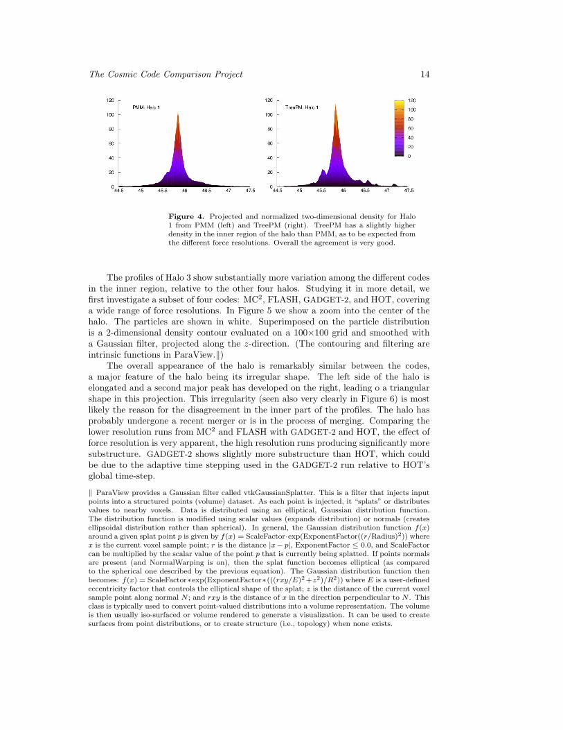
Next we investigate the correlation of the numbers of halos with density (measuredby the number of particles per grid cell on a 323 grid). The results for six codes areshown in Figure 12. The results for the four other codes are very similar comparedto the codes using the same algorithm (e.g. the FLASH result is very close to theEnzo result). The scatter plots show three different mass bins: very light halos (10-40particles) in red, medium mass halos (41-2500 particles) in green, and the heaviesthalos in the simulations (2500 and more particles) in blue. These thresholds werechosen because, as discussed earlier, the force resolution of MC2 and PMM shouldbe sufficient to resolve halos with more than 40 particles, while Enzo’s and FLASH’sbase grid set this limit to more than 2500 particles. The green and blue crosses areslightly shifted upward to make all points visible. The cut-offs on the left of the scatterplots are easy to understand: a certain minimum density is required to have a haloof a certain size and a certain number of halos, e.g. 50 small halos cannot live inan underdense cell. Enzo and TPM show the largest deficit of halos, confirming themass function results. The small halos in Enzo are mainly missing in the low densityregions, and below δVoid there are almost no halos. TPM has a very large deficitbetween 1,000-10,000 particles per cell, corresponding to a density contrast δ between1 and 20. This confirms the visual impression from Figure 10. The overall agreementespecially for the larger halos is very good. The largest halo (blue cross on the farright) seems to be surrounded by a large number of small halos, consistent among allcodes.

To cast the results from Figure 12 in a more quantitative light, Figure 13 displaysthe distribution of halos with respect to density for the two lower mass bins. From


Figure 12. Correlation between the particle density (calculated on a 323 grid)and the numbers of halos in a certain density regime. The smallest halos (10-40particles) are marked in red, medium size halos (41-2500 particles) are shown ingreen, and the biggest halos (more than 2500 particles) are shown in blue. Thegreen crosses are shifted by 0.15 and the blue crosses by 0.3 upwards to make allpoints visible.


1

10

100

1000

Num

ber o

f Hal

os

MC2PMMEnzo

FLASHHOT

PKDGRAVHydra

Gadget-2TPM

TreePM 1

10

100

1000

Num

ber o

f Hal

os

MC2PMMEnzo

FLASHHOT

PKDGRAVHydra

Gadget-2TPM

TreePM

0

0.2

0.4

0.6

0.8

1

1.2

1.4

100 1000 10000 100000

Ratio

s

Number of Particles per Grid Block

0

0.2

0.4

0.6

0.8

1

1.2

1.4

1.6

1.8

10 100 1000 10000 100000

Ratio

s

Number of Particles per Grid Block

Figure 13. Number of halos as a function of density. Left panel: halos with10 - 40 particles, right panel: halos with 41 - 2500 particles. The lower panelsshow the residuals with respect to GADGET-2. Both panels show the deficit ofsmall halos in Enzo and FLASH over most of the density region – only at veryhigh densities do the results catch up. The behavior of the TPM simulation isinteresting: not only does this simulation have a deficit of small halos but thedeficit is very significant in medium density regions, in fact falling below the twoAMR codes. The slight excess of small halos shown in the TreePM run vanishescompletely if the halo cut is raised to 20 particles per halo and the TreePM resultsare in that case in excellent agreement with GADGET-2.

Figure 12 we can read off the density range of interest for each mass bin, i.e. thedensity range with the largest halo population. We restrict our investigations to adensity threshold of up to 100,000 particles per cell. Figure 13 shows the results for10-40 particle (left panel) and 41-2500 particle halos (right panel). The lower panelsshow the residuals with respect to GADGET-2. (We have verified that the agreementfor larger halos between the ten codes is very good as expected from Figure 12.) Thetwo AMR codes Enzo and FLASH have a deficit for both halo sizes over most of thedensity region. They only catch up with the other codes at around 10,000 particles percell, in agreement with the our previous argument that whether halos are resolvableby the AMR codes or not is dictated by the size of the base grid. In terms of capturingsmaller halos, the refinement only helps in very high density regions.

The result for the TPM simulation is somewhat paradoxical: in the low density


region the result for the small halos agrees well with the other high-resolution codes,however, TPM misses a very large number of small halos in the region between 200 and10,000 particles per cell, the curve falling even below the AMR codes. This suggeststhat the problem of the TPM code is not due to the threshold criterion for the tree butperhaps due to a hand-over problem between the grid and the tree. The two PM codeshave slightly lower numbers of very small halos, in good agreement with the predictionthat they only resolve halos with more than 40 particles. The agreement between MC2

and PMM itself is excellent. The TreePM code shows a slight excess of small haloscompared to the other high-resolution codes. This excess vanishes completely if the cutfor the small halos is chosen to be 20 particles instead of 10 particles for the smallestallowed halo. This indicates a slightly higher force resolution in the TreePM runcompared to the other runs. The agreement for the medium size halos (left panel) isvery good, except for the AMR codes. For the medium size halos, the TPM code againshows a slight deficit of halos in the medium density regime, but far less pronouncedthan for the small halos. The overall agreement of the high-resolution codes is verygood, as is to be expected from the mass function results.

5.4. The Power Spectrum

The matter power spectrum is one of the most important statistics for precisioncosmology. Upcoming weak lensing surveys promise measurements of the powerspectrum at the one percent accuracy level out to length scales of k ∼ 10hMpc−1

(for an overview of the requirements for the accuracy of predictions for future lensingsurveys, see, e.g., Ref. [57]). This poses a severe theoretical challenge: predicting thematter power spectrum at the same level of accuracy. A first step for showing that thisis possible is to investigate how well the matter power spectrum can be predicted frompure dark matter simulations, baryonic physics being included as a second step. Ithas already been shown that at the length scales of interest, hydrodynamic effects canalter the matter power spectrum at up to 10 percent [58]. In this paper we concentrateon the first step and determine how well a diverse set of N-body codes agree with eachother for the prediction of the matter power spectrum. In future work we aim topredict the dark matter power spectrum at k ∼ 1hMpc−1 at the level of one percentaccuracy or better. This will include a detailed analysis of the accuracy of the initialconditions as well as of the nonlinear evolution, a task beyond the scope of the currentpaper.

We determine the matter power spectrum by generating the density field from theparticles via a Cloud-in-Cell (CIC) routine on a 10243 spatial grid and then obtain thedensity in k-space by applying a 10243 FFT. The square of the k-space density yieldsthe power spectrum: P (k) = 〈|δ(k)2|〉. The CIC routine introduces a filter at smalllength scale. We compensate for this filtering artifact by deconvolving the k-spacedensity with a CIC window function.

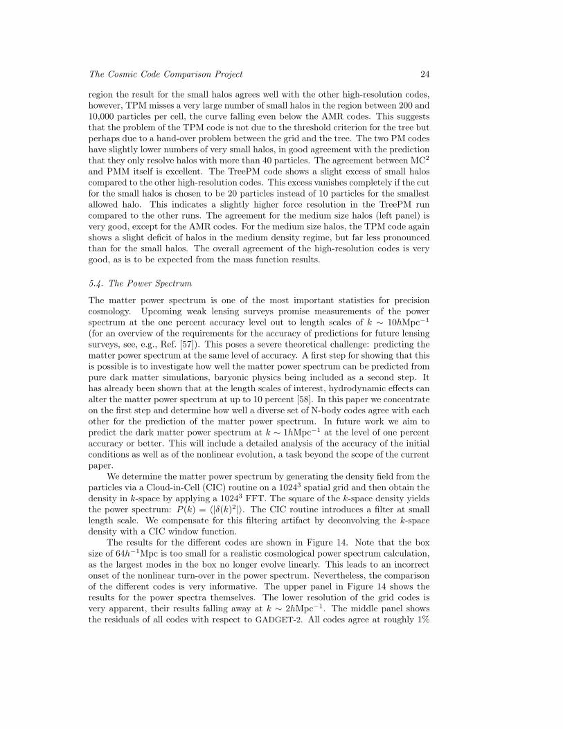
The results for the different codes are shown in Figure 14. Note that the boxsize of 64h−1Mpc is too small for a realistic cosmological power spectrum calculation,as the largest modes in the box no longer evolve linearly. This leads to an incorrectonset of the nonlinear turn-over in the power spectrum. Nevertheless, the comparisonof the different codes is very informative. The upper panel in Figure 14 shows theresults for the power spectra themselves. The lower resolution of the grid codes isvery apparent, their results falling away at k ∼ 2hMpc−1. The middle panel showsthe residuals of all codes with respect to GADGET-2. All codes agree at roughly 1%


Figure 14. Power spectrum results and the residuals for the different codes.Upper panel: comparison of the different power spectra. Middle panel: residualsof all codes with respect to GADGET-2. Lower panel: Residuals of the meshcodes with respect to MC2.

out to k ∼ 1hMpc−1. PKDGRAV shows small scatter in the linear regime. Thismight be caused by imprecise periodic boundary conditions, which are not as easy toimplement in tree codes as they are for grid codes. The high-resolution codes agreeto better than 5% out to k ∼ 10hMpc−1. At that point HOT and Hydra lose power,while PKDGRAV, TPM, and TreePM show slightly enhanced power compared to theGADGET-2 run. The formal force resolutions of the codes would suggest that thedifferent runs (including the grid runs) should agree much better at the wavenumbersshown.

The 10243 FFT used to generate the power spectra is far below the resolutionof the non-grid codes and at the resolution limit of the AMR and PM codes. Thediscrepancy might be due to several reasons: the number of time steps, the accuracy ofthe force solvers, the accuracy of reaching z = 0 at the end of each run, just to suggesta few. A more detailed study of the power spectrum including larger simulation boxesis certainly required to obtain the desired accuracy for upcoming surveys. In the lowerpanel we show a comparison of the grid codes only, with respect to MC2. The twopure PM codes, MC2 and PMM agree remarkably well over the whole k-range underconsideration, the difference being below 1%. The two AMR codes, Flash and Enzo,deviate considerably, most likely due to different refinement criteria. It is somewhatsurprising that Enzo has larger power than the two PM codes, which have the sameresolution in the whole box that Enzo has only in high density regions. This could bethe result of an algorithmic artifact in the AMR implementation.


To summarize, the agreement for the matter power spectrum is at the 5% levelover a large range in length scale. The early deviation of the grid codes is surprising, asthe nominal resolution of all codes should have been sufficient to generate agreementover a wider k-range. In order to be able to obtain more cosmologically relevantresults at k ∼ 1hMpc−1, much larger simulation boxes have to be compared. Athigher wavenumbers, baryonic effects become important leading to the necessity of amuch more involved comparison set-up.

6. Conclusion and Discussion

The new era of precision cosmology requires new standards for the reach andaccuracy of large cosmological simulations. While previously, qualitative answers andquantitative results at the 20% accuracy level were sufficient, we now need to robustlypredict nonlinear physics at the 1% accuracy level. This demanding task can only beachieved by rigorous code verification and error control.

In this paper we have carried out a comprehensive code comparison project with10 state-of-the-art cosmological simulation codes. ParaView was introduced as apowerful analysis tool which should make it more convenient for code developersto compare results. In particular, results from the current suite of simulations canfunction as a good database for reference purposes and benchmarking. The initialconditions are publicly available+.

The results from the code comparisons are satisfactory and not unexpected, butalso show that much more work is needed in order to attain the required accuracy forupcoming surveys. The halo mass function is a very stable statistic, the agreementover wide ranges of mass being better than 5%. Additionally, the low mass cutoff forindividual codes can be reliably predicted by a simple criterion.

The internal structure of halos in the outer regions of ∼ R200 also appears to bevery similar between different simulation codes. Larger differences between the codesin the inner region of the halos occur if the halo is not in a relaxed state: in thiscase, time stepping issues might also play an important role (e.g. particle orbit phaseerrors, global time mismatches). For halos with a clear single center, the agreement isvery good and predictions for the fall-off of the profiles from resolution criteria holdas expected. The investigation of the halo counts as a function of density revealed aninteresting problem with the TPM code, the simulation suffering from a large deficitin medium density regimes. The AMR codes showed a large deficit of small halos overalmost the entire density regime, as the base grid of the AMR simulation set too lowa resolution limit for the halos.

The power spectrum measurements revealed definitely more scatter among thedifferent codes than expected. The agreement in the nonlinear regime is at the 5-10%level, even on moderate spatial scales around k = 10hMpc−1. This disagreement onsmall scales is connected to differences of the codes in the inner regions of the halos.

Acknowledgments

The calculations described herein were performed in part using the computationalresources of Los Alamos National Laboratory. A special acknowledgment is due+ http://t8web.lanl.gov/people/heitmann/arxiv


to supercomputing time awarded to us under the LANL Institutional ComputingInitiative.

References

[1] Zel’dovich, Y.B. 1970, A&A, 5, 84; Shandarin, S. and Zel’dovich, Y.B. 1989, Rev. Mod. Phys.61, 185.

[2] Heitmann, K., Ricker, P.M., Warren, M.S., & Habib, S. 2005, ApJS, 160, 28.[3] Ryne, R.D., Habib, S., Qiang, J., Ko, K., Li, Z., McCandless, B., Mi, W., Ng, C.-K., Saparov, M.,

Srinivas, V., Sun, Y., Zhan, X., Decyk, V., & Golub, G. 1998, The US DOE Grand Challengein Computational Accelerator Physics, Proceedings LINAC98 (Chicago, IL).

[4] Qiang, J., Ryne, R.D., Habib. S., and Decyk, V. 2000, J. Comp. Phys., 163, 434.[5] Trac, H. and Pen, U.-L. 2006, New Astron., 11, 273.[6] Bryan, G.L. and Norman, M.L. 1996, 12th Kingston Meeting on Theoretical Astrophysics,

proceedings of meeting held in Halifax; Nova Scotia; (ASP Conference Series # 123), D.A.Clarke. and M. Fall.

[7] Bryan, G.L. and Norman, M.L. 1999, Workshop on Structured Adaptive Mesh Refinement GridMethods, ed. N. Chrisochoides (IMA Volumes in Mathematics No. 117)

[8] O’Shea, B.W., Bryan, G., Bordner, J., Norman, M.L., Abel, T., Harkness, R. and Kritsuk,A. 2004, Adaptive Mesh Refinement - Theory and Applications, T. Plewa, T. Linde and G.Weirs, Springer-Verlag.

[9] O’Shea, B.W., Nagamine, K., Springel, V., Hernquist, L., and Norman, M.L. 2005, ApJS, 160,1.

[10] Berger, M.J. and Colella, P. 1989, 82, 64.[11] Efstathiou, G., Davis, M., White, S.D.M., and Frenk, C.S. 1985, ApJS, 57. 241.[12] Hockney, R.W. and Eastwood, J.W. 1988, Computer Simulation Using Particles, Institute of

Physics Publishing.[13] Woodward, P.R. and Colella, P. 1984, J. Comp. Phys., 54, 174.[14] Bryan, G.L., Norman, M.L., Stone, J.M., Cen, R., and Ostriker, J.P. 1995, Comp. Phys. Comm.,

89, 149.[15] Fryxell, B., et al. 2000, ApJS, 131, 273.[16] MacNeice, P., Olson, K.M., Mobarry, C., de Fainchtein, R., and Packer, C. 2000, CPC, 126, 330.[17] Quirk, J.J. 1991, PhD thesis, Cranfield Institute of Technology.[18] de Zeeuw, D. and Powell, K.G. 1993, JCP, 104, 56.[19] Warren, M.S. and Salmon, J.K. 1993, in Supercomputing ’93, 12, Los Alamitos IEEE Comp.

Soc.[20] Salmon, J.K. and Warren, M.S. 1994, J. Comp. Phys., 111, 136.[21] Warren, M.S, Fryer, C.L., and Goda, M.P. 2003, in Proceedings of the ACM/IEEE SC2003

Conference (ACM Press, New York).[22] Frenk, C.S., et al. 1999, ApJ, 525, 554.[23] Fryer, C.L., and Warren, M.S. 2002, ApJ, 574, L65.[24] Dikaiakos, M.D. and Stadel, J. 1996, ICS Conference Proceedings.[25] Barnes, J. and Hut, P. 1986, Nature, 324, 446.[26] Hernquist, L., Bouchet, F., and Suto Y. 1991, ApJS, 75, 231.[27] Couchman, H.M.P. 1999, J. Comp. App. Math., 109, 373.[28] Springel, V., Yoshida, N., and White, S.D.M. 2001, New Astronomy, 6, 79.[29] Springel, V. 2005, MNRAS, 364, 1105.[30] Bagla, J.S. 2002, J. of Astrophysics and Astronomy, 23, 185.[31] Monaghan, J.J. 1992, Ann. Rev. Astron. Astrophys.30, 543.[32] Springel, V. and Hernquist, L. 2002, MNRAS, 333, 649.[33] Xu, G. 1995, ApJS, 98, 355.[34] Bode, P., Ostriker, J.P., and Xu, G. 2000, ApJS, 128, 561.[35] White, M. 2002, ApJS, 143, 241.[36] Klypin, A.A. and Holtzman, J. 1997, astro-ph/9712217.[37] Bardeen, J.M., Bond, J.R., Kaiser, N., and Szalay, A.S. 1986, ApJ, 304, 15.[38] Dehnen, W. 2001, MNRAS, 324, 273.[39] Ahrens J., Geveci B., and Law C., “ParaView: An End-User Tool for Large Data Visualization”,

in C. Hansen and C. Johnson, editors, The Visualization Handbook, pages 717-731, AcademicPress, 2005.

[40] Lacey, C. and Cole, S. 1994, MNRAS, 271, 676.

http://arXiv.org/abs/astro-ph/9712217


[41] Davis, M., Efstathiou, G., Frenk, C.S. 1985, ApJ, 292, 371.[42] Navarro, J.F., Frenk C.S., & White, S.D.M. 1995, MNRAS, 267, 401.[43] Bullock, J.S. et al. 2001, MNRAS, 321, 559, and references therein.[44] Majumdar S. and Mohr J.J. 2004, ApJ, 613, 41 and references therein.[45] Press, W.H. and Schechter, P. 1974, ApJ, 187, 425.[46] Lee, J. and Shandarin, S. 1998, ApJ, 500, 14[47] Sheth, R.K., Mo, H.J., and Tormen, G. 2001, MNRAS, 323, 1.[48] Sheth, R.K. & Tormen, G. 1999, MNRAS, 308, 119.[49] Jenkins, A. et al. 2001, MNRAS 321, 372.[50] Warren, M.S., Abazajian, K., Holz, D.E., and Teodoro, L. 2006, ApJ, 646, 881.[51] Reed, D. et al. 2003, MNRAS, 346, 565.[52] Reed, D., Bower, R., Frenk, C., Jenkins, A. and Theuns T. 2007, MNRAS, 374, 2.[53] Heitmann, K., Lukic, Z., Habib, S., and Ricker, P.M. 2006, ApJ, 642, L85.[54] Lukic, Z., Heitmann, K., Habib, S., Bashinsky, S., and Ricker, P.M. 2007, astro-ph/0702360.[55] Barkana, R. & Loeb, A. 2004, ApJ, 609, 474.[56] Bagla, J.S. and Prasad, J. 2006, MNRAS, 370, 993.[57] Huterer, D. and Takada, M. 2005, Astropart. Phys., 23, 369.[58] Zhan, H. and Knox, L. 2004, ApJL, 616, L75; White, M. 2004, Astropart. Phys., 22, 211; Jing,

Y.P., Zhang, P., Lin, W.P., Gao, L., and Springel, V. 2006, ApJL, 640, 119; Rudd, D.H.,Zentner, A.R., and Kravtsov, A. 2007, astro-ph/0703741.



LA-UR- - Data science · LA-UR- Approved for public release; distribution is unlimited. Los Alamos...

Documents

Transcript of LA-UR- - Data science · LA-UR- Approved for public release; distribution is unlimited. Los Alamos...