La Dottora Ricer in Ingegneria Inf orma tica XIV Ciclodottoratoii/media/students/... ·...

Universit�a degli Studi di Roma \La Sapienza"

Dottorato di Ricerca in Ingegneria Informatica

XIV Ciclo { 2001

Scheduling Algorithms and Localization Tools

for

Wireless Networks

Andrea Vitaletti


Dottorato di Ricerca in Ingegneria Informatica

XIV Ciclo - 2001

Andrea Vitaletti

Scheduling Algorithms and Localization Tools

for

Wireless Networks

Thesis Committee

Prof. Alberto Marchetti Spaccamela (Advisor)

Prof. Stefano Leonardi

Prof. Giancarlo Bongiovanni

Author's address:

Andrea Vitaletti

Dipartimento di Informatica e Sistemistica


Via Salaria 113, I-00198 Roma, Italy

e-mail: [email protected]

www: http://www.dis.uniroma1.it/�vitale

i

Preface

I started my Ph.D. mainly for one reason and with two objectives in mind. The reason was

that I like science, particularly in its technological implications, and I love to be free of studying

and exploring what I like. \Personalmente amo investigare liberamente la verit�a di quelle a�er-

mazioni che mi arrecano piacere"1. This phrase by Sagredo, a good friend of Galileo, e�ectively

expresses what I mean. The objectives were to learn as many things as possible while explor-

ing new solutions, and to show that a stronger cooperation between industry and university is

possible. Now, after three years, I can say that the reason was a good one, and that I achieved,

in my own small way, both my objectives. This is somehow testi�ed by some publications

[26, 59, 54, 75, 69, 51] and three United States provisional patent applications [72, 74, 73].

Acknowledgments

Many friends supported me during these Ph.D. years; I love to say that it is always better to

work with friends rather than simply with colleagues.

First I wish to thank Alberto Marchetti-Spaccamela and Stefano Leonardi, I learned a lot

from them. I met both of them during the last year in my computer science classes.

I still remember when Alberto during the last lesson of his course in networking said, \... no

matter who is the professor and which is the subject of your thesis, it is more important you do

something you like ...". Simply the truth.

Stefano is a brilliant computer scientist, and his door has been always open for encouragement

and suggestions. More importantly, we had great time eating and drinking 2 together. Wherever

you are in the world, he always knows which is the best dish and the appropriate wine.

Thanks also to Luca Becchetti, because the musketeers are always three ... Alexander Dumas

docet.

I am grateful to Giorgio Ausiello and Bruno Errico. Both of them, from a di�erent perspective

(academic Giorgio and industrial Bruno) gave me the same suggestion when I was dubious in

starting my Ph.D., \... It is up to you, but for sure Ph.D. is a great experience ...".

1\Personally I love to freely investigate the truth of those assertions that enjoy myself", from \Galileo. A life",

James Reston Jr, Harper Collins Publishers, New York, 1994 .2Romans said: \in vino veritas", \In wine the truth".

ii

Thanks to Etnoteam, the company for which I still work, because it gave me enough freedom

to do my Ph.D. ... not usual for an Italian company.

Thanks to my AT&T friends Muthu, Rittwik, Ted and Suhas. My stay in the AT&T research

labs was really a great experience. In particular thanks to Muthu, for giving me this opportunity

and for his infectious joy of living.

Thanks to Camil and Luigi, my roommates. It is not easy to have me and my confusion in

the same room.

I thank Stefano, Alberto and Giancarlo Bongiovanni, for serving on my Ph.D. committee.

Thanks to the reviewers Danny Raz, Kirk Prhus and Vincenzo Liberatore, for their sugges-

tions and comments.

I wish to thank also my family and all the other friends for their constant encouragement

and moral support.

Finally thanks to Chiara, my wife, because she helps me to be what I am.

Contents

1 Introduction 1

1.1 Wireless Internet Applications . . . . . . . . . . . . . . . . . . . . . . . . . . . . . 2

1.2 Quality of Services for new wireless applications . . . . . . . . . . . . . . . . . . 4

1.3 Wireless Scheduling . . . . . . . . . . . . . . . . . . . . . . . . . . . . . . . . . . 5

1.4 Overview of the Thesis . . . . . . . . . . . . . . . . . . . . . . . . . . . . . . . . . 7

1.4.1 Suited: A Prospect of QoS Enabled Wireless Communication and Services 7

1.4.2 Scheduling problems . . . . . . . . . . . . . . . . . . . . . . . . . . . . . . 8

1.4.3 System architecture for location based services . . . . . . . . . . . . . . . 11

2 Suited: A Prospect of QoS Enabled Wireless Communication and Services 13

2.1 Suited and the GMBS . . . . . . . . . . . . . . . . . . . . . . . . . . . . . . . . . 14

2.1.1 Wireless Technologies . . . . . . . . . . . . . . . . . . . . . . . . . . . . . 14

2.1.2 Internet Service Requirements . . . . . . . . . . . . . . . . . . . . . . . . 18

2.1.3 Federated ISP and the nowadays Internet . . . . . . . . . . . . . . . . . . 22

2.2 Suited System Architecture . . . . . . . . . . . . . . . . . . . . . . . . . . . . . . 23

2.2.1 Edge Network . . . . . . . . . . . . . . . . . . . . . . . . . . . . . . . . . . 24

2.2.2 Core Network . . . . . . . . . . . . . . . . . . . . . . . . . . . . . . . . . . 25

2.2.3 Mobility . . . . . . . . . . . . . . . . . . . . . . . . . . . . . . . . . . . . . 26

3 Downlink Scheduling for Multirate Wireless Networks 29

3.1 Problem Formulation . . . . . . . . . . . . . . . . . . . . . . . . . . . . . . . . . . 30

3.1.1 Wireless Network Model . . . . . . . . . . . . . . . . . . . . . . . . . . . . 30

3.1.2 Communication Channel Model . . . . . . . . . . . . . . . . . . . . . . . . 31

3.1.3 Overview of Next Generation Wireless Multirate Data Networks . . . . . 32

iii

iv CONTENTS

3.1.4 Abstract Scheduling Problem . . . . . . . . . . . . . . . . . . . . . . . . . 35

3.2 Understanding the Scheduling Problems . . . . . . . . . . . . . . . . . . . . . . . 37

3.2.1 Some Structural Observations . . . . . . . . . . . . . . . . . . . . . . . . . 37

3.2.2 Computational Hardness. . . . . . . . . . . . . . . . . . . . . . . . . . . . 39

3.2.3 O�ine scheduling problem . . . . . . . . . . . . . . . . . . . . . . . . . . . 40

3.3 Online Heuristics . . . . . . . . . . . . . . . . . . . . . . . . . . . . . . . . . . . . 44

3.3.1 The discrete case . . . . . . . . . . . . . . . . . . . . . . . . . . . . . . . . 49

3.4 Simulation Study . . . . . . . . . . . . . . . . . . . . . . . . . . . . . . . . . . . . 55

3.4.1 Experiments . . . . . . . . . . . . . . . . . . . . . . . . . . . . . . . . . . 57

3.5 Related Work . . . . . . . . . . . . . . . . . . . . . . . . . . . . . . . . . . . . . . 61

3.6 Conclusions . . . . . . . . . . . . . . . . . . . . . . . . . . . . . . . . . . . . . . . 62

4 Bandwidth and Storage Allocation Problems under Real Time Constraints 63

4.1 The RP problem . . . . . . . . . . . . . . . . . . . . . . . . . . . . . . . . . . . . 66

4.2 A LP based approximation algorithm . . . . . . . . . . . . . . . . . . . . . . . . 66

4.2.1 The LP formulation . . . . . . . . . . . . . . . . . . . . . . . . . . . . . . 67

4.2.2 The algorithm for obtaining a stable solution . . . . . . . . . . . . . . . . 68

4.2.3 Constructing a feasible solution . . . . . . . . . . . . . . . . . . . . . . . . 71

4.2.4 A strongly polynomial time algorithm . . . . . . . . . . . . . . . . . . . . 74

4.3 A combinatorial algorithm . . . . . . . . . . . . . . . . . . . . . . . . . . . . . . . 76

4.4 The multiple channel case . . . . . . . . . . . . . . . . . . . . . . . . . . . . . . . 78

4.5 Conclusions . . . . . . . . . . . . . . . . . . . . . . . . . . . . . . . . . . . . . . . 78

5 Randomized Lower Bounds for Online Path Coloring 79

5.1 A lower bound for online interval graph coloring . . . . . . . . . . . . . . . . . . 82

5.1.1 The probability distribution . . . . . . . . . . . . . . . . . . . . . . . . . . 83

5.1.2 The proof of the lower bound . . . . . . . . . . . . . . . . . . . . . . . . . 83

5.2 A lower bound for online path coloring on trees . . . . . . . . . . . . . . . . . . . 89

5.3 Conclusions . . . . . . . . . . . . . . . . . . . . . . . . . . . . . . . . . . . . . . . 95

6 System Architecture for Location Based Services 97

6.1 Localization Technology . . . . . . . . . . . . . . . . . . . . . . . . . . . . . . . . 98

6.2 CDPD Architecture . . . . . . . . . . . . . . . . . . . . . . . . . . . . . . . . . . 100

CONTENTS v

6.3 The MSCI Protocol . . . . . . . . . . . . . . . . . . . . . . . . . . . . . . . . . . 101

6.4 The GEOPROXY Architecture . . . . . . . . . . . . . . . . . . . . . . . . . . . . 103

6.5 Accuracy . . . . . . . . . . . . . . . . . . . . . . . . . . . . . . . . . . . . . . . . 105

6.5.1 GPS measurement . . . . . . . . . . . . . . . . . . . . . . . . . . . . . . . 106

6.5.2 Average distance . . . . . . . . . . . . . . . . . . . . . . . . . . . . . . . . 107

6.5.3 Service Accuracy . . . . . . . . . . . . . . . . . . . . . . . . . . . . . . . . 109

6.6 Techniques to improve BSIC method accuracy . . . . . . . . . . . . . . . . . . . . 112

6.6.1 Accuracy improvement using multiple cells . . . . . . . . . . . . . . . . . 112

6.6.2 Accuracy improvement using RSSI . . . . . . . . . . . . . . . . . . . . . . 114

6.7 Conclusions and Future Works . . . . . . . . . . . . . . . . . . . . . . . . . . . . 117

vi CONTENTS

Chapter 1

Introduction

The Internet protocol architecture was originally conceived with the main objective of creating

a robust and scalable infrastructure able to support the deployment of a number of applications.

The Internet users were assumed to be in a steady state, at the oÆce, at home etc., and

accessing the network by means of wired links. Moreover services and applications, mostly

required a reliable end-to-end data transfer, satisfactorily supported by a best e�ort service

model. The Internet network described above is no more suitable to face the emerging needs

of a new population of Internet nomadic users (see Figure 1.1), such as travellers on wheels,

on water or in the air, who desire to gain access to multimedia services regardless of their

location and, if possible, while in motion. The deployment of a system capable to support

the ubiquitous Internet, may bene�t from the cooperation of a variety of wireless technologies,

such as Wireless Lan, cellular network (GSM/GPRS/UMTS) and satellite networks. In fact

neither wireless terrestrial networks nor satellite systems operating by themselves are able to

serve the high diversi�ed environments foreseen in the ubiquitous Internet, such as the open

rural environment, the suburban/urban environment and the indoor and low-range outdoor

environment. The design of a network architecture capable of exploiting and integrating the

characteristics of the above wireless technologies is one of the most challenging objective of next

generation wireless networks (see Chapter 2).

1

2 CHAPTER 1. INTRODUCTION

Today Ubiquity

Reachability

Security

Convenience

Tomorrow Localization

Instant Connectivity

Personalization

Table 1.1: Attributes of Mobile Communication

1.1 Wireless Internet Applications

A recent study [56] indicates the attributes in Table 1.1 as the key drivers for the increasing

sophistication of the mobile market.

In the following we give a brief explanation of these attributes. Ubiquity: it is the most

obvious advantage of a wireless terminal. A mobile terminal in the form of a smart phone

or a communicator can ful�ll the need both for real-time information and for communication

anywhere, independent of the users location. Reachability: with a mobile terminal a user can

be contacted anywhere anytime. Security: mobile security technology is already emerging in

the form of SSL (Secure Socket Layer) technology. Furthermore the smartcard within the

terminal, the SIM (Subscriber Identi�cation Module) card, provides authentication of the owner

and enables a higher level security than currently is typically achieved in the �xed internet

environment. Convenience: it is an attribute that characterizes a mobile terminal. Devices

store data, are always at hand and are increasingly easy to use. Instant Connectivity: instant

connectivity to the internet from a mobile phone is becoming a reality already and will fast-

forward with the introduction of GPRS services. With WAP or any other microbrowser over

GSM, a call to the internet has to be made before applications can be used. Using GPRS it

will be easier and faster to access information on the web without booting a PC or connecting

a call. Personalisation: personalisation is, to a very limited extent, already available today.

However, the emerging need for payment mechanisms, combined with availability of personalised

information and transaction feeds via mobile portals, will move customisation to new levels,

leading ultimately to the mobile device becoming a real life-tool.

Finally Localization: the ability to locate the position of a mobile device is considered crucial

1.1. WIRELESS INTERNET APPLICATIONS 3

Figure 1.1: Source: Dataquest, Mobile Commu-

nications International.

Figure 1.2: Data application are critical. Source:

Microsoft.

for providing geographically speci�c value-added information. Applications using mobile location

service technologies include eet management, vehicle tracking for security, tracking for recovery

in event of theft, telemetry, emergency services, location identi�cation, navigation, location

based information services and location based advertising. The largest push for localization

technology is coming from the US. There, mobile telephone operators have been forced by the

FCC to provide emergency 911 services by October 2001 in such a way that the location of

the caller could be determined within a radius of 125 meters in 67% of all cases. There are

three major localization techniques: 1) Triangulation can be done via lateration, which uses

multiple distance measurements between known points, or via angulation, which measures angle

or bearing relative to points with known separation; 2) Proximity measures nearness to a known

set of points; 3) Scene analysis examines a view from a particular vantage point, such as antennae

or mobile terminals. Implementation of location systems generally uses one or more of these

techniques to locate objects and people. Furthermore location systems can be either terminal

based or network based. In terminal based systems, it is the mobile device itself that determines

the location. Normally these systems are less accurate but they do not require signi�cant network

upgrade. Network based systems provide more accurate localization information, but require a

signi�cant upgrade of the network. In chapter 6 of this thesis we present our terminal based

localization technique. This technique is protected by three United States provisional patent

applications ([72], [74], [73]).


1.2 Quality of Services for new wireless applications

With mobile communications reaching the mass market, network operators are facing decreasing

ARPU (Average Revenue Per User, See Figure 1.2). The network operators must then contin-

uously implement new services on their network. These new services (mainly data services)

often require a suitable Quality of Services (QoS). Nowadays users are not simply satis�ed by

the availability of the service itself, they want to experience a good QoS. A real time appli-

cation, such as for example video conference, not only imposes strict requirements in terms of

bandwidth, but also in terms of packet delay (normally should be less than 400ms) and jitter

(jitter is the variation of delay and should be almost constant). On the contrary, a File Transfer

application, has mainly requirements in terms of bandwidth, being extremely tolerant to high

delay and variable jitter. The heterogeneous nature of the Internet applications, requires an

e�ort in developing a network infrastructure capable of addressing such requirements.

The best e�ort QoS currently available over the Internet, is unable to e�ectively cope with these

requirements. From a best e�ort point of view, each IP packet is handled in the same way,

independently if it has been generated from a real time application, rather than from a simple

FTP. All the IP packets scheduled by a router, are queued in the same queue and are typically

served according to a FIFO policy; thus Real time traÆc may be delayed because of the presence

of a huge number of FTP packets. In a best e�ort network, the only way to guarantee the QoS

is over-dimensioning network links, in order to avoid traÆc congestion.

A �rst solution proposed to address the above problems is the introduction of the Di�Serv ar-

chitecture. In Di�Serv, each packet is classi�ed according to a speci�c classi�cation policy, for

example distinguishing among real time packets and FTP packets. Each packet in a speci�c

class is handled according to a particular scheduling algorithm. For example, real time packets

can have a priority over FTP packets. In such a way the delay accumulated by real time packets

is not anymore in uenced by the presence of FTP packets. Note however that this architecture

does not avoid the generation of delay within the real time class itself. In other words, if the

number of real time sessions become too high, it is still possible the accumulation of a huge

delay. Although Di�Serv is a simple and scalable solution o�ering a \better than best e�ort"

QoS, it potentially su�ers of the same problem of congestion of best e�ort. A further solution

capable of addressing this problem, is the IntServ architecture. The IntServ architecture, ex-

pects that each new communication ow reserves in advance (for example through the RSVP

1.3. WIRELESS SCHEDULING 5

protocol) the resources for providing a suitable QoS. In other words, the system checks if it has

enough resources to manage the new communication and to simultaneously maintain a suitable

QoS for the ongoing communications. If those resources are available, the new communication

is accepted, on the contrary it is refused or it is accepted with a reduced QoS compatible with

the available resources. Although IntServ e�ectively provide an \hard QoS" to the accepted

communications, because of its per- ow orientation is extremely resource consuming and can

be applied only within small scale networks. For this reason, it has been proposed an hybrid

approach taking advantage from the cooperation of IntServ and Di�Serv (see Chapter 2).

In this thesis we mainly focus on network layer QoS, nevertheless similar issues arise at link

layer. Cooperation between network and link layers to achive overall QoS is in part still an open

problem.

1.3 Wireless Scheduling

A relevant part of the above cited QoS mechanisms is taken by traÆc scheduling policies, at

which is dedicated a considerable part of this thesis (see Chapters 3, 4 and 5). A scheduling

algorithm allocates resources to communication requests in order to minimize/maximize an ob-

jective function that normally describes the QoS experienced by the users. As we have seen

above, it is a scheduling algorithm that, according to a speci�c scheduling policy (from the sim-

ple FIFO in best e�ort to the more complicated priority queuing in Di�Serv enabled routers),

schedules the next packet to be served in a router.

In the following we introduce the main characteristics of scheduling algorithms focusing on the

peculiarity of the wireless environment. We have seen that the demand for wireless commu-

nication systems is continuously growing (see Figure 1.1). Since wireless frequency is a scarce

resource, eÆcient frequency utilization is a relevant issue; although new wireless technology

greatly increase the bandwidth availability of wireless systems, this is still a limited fraction of

the bandwidth available in wireline networks. Resource allocation schemes and scheduling poli-

cies are critical to optimize frequency utilization. However, resource allocation and scheduling

schemes from the wireline domain cannot be directly applied to wireless system, since wireless

channels have unique characteristics, such as limited bandwidth, time-varying and location-

dependent channel condition and channel-condition-dependent throughput. In particular, if we


consider the radio propagation, it can be roughly characterized by three nearly independent

phenomena: path-loss variation with distance (path losses vary with the movement of mobile

stations), slow log-normal shadowing and fast multipath-fading. The last two characteristic are

time-varying and they imply that users perceive time-varying service quality. For voice users,

better channel conditions may results in better voice quality. For data users, better channel

condition can be used to provide higher data rates. A good scheduling scheme should be able

to exploit the time-varying channel conditions of users to achieve higher utilization of wireless

resources. Nevertheless the potential to exploit higher data throughput introduces the trade-o�

problem between wireless resource eÆciency and fairness among users. Since wireless spectrum

is a scarce resource, improving the eÆciency of spectrum utilization is a crucial issue. However

a scheme designed only to maximize the overall throughput could be unfair among users. For

example allowing only users with good channel condition to transmit with high transmission

power may result in a very high throughput, but it is unfair to other users. In this thesis we

will mainly consider objective functions that express user satisfaction. For example we will con-

sider minimizing the maximum or average response time (the response time is the time elapsed

between the release of a request and its completion). Other possible objective functions are

minimizing the total weighted response time, or minimizing maximum or total stretch (whereas

the stretch of a job is the ratio between its ow time and its processing time or size).

The scheduling problem that we consider are NP-hard optimization problems and, therefore, we

do not expect to solve them exactly in polynomial time. For this reason we are interested in

algorithms that provide us an approximate solution in polynomial time. We will measure the

quality of the approximate solution using both an experimental approach and/or evaluating the-

oretically the performance obtained by the algorithms. Scheduling algorithms can be considered

in two main variants, namely o�ine and online. The o�ine version of a scheduling problem

assume that all requests are known in advance before being served. Hence the o�ine algorithm

has a full knowledge of the future requests and can schedule them in the most appropriate way

in order to minimize/maximize the objective function. The o�ine case is of theoretical interest

and is mainly useful to quantify the bene�t to be accrued from scheduling, that in most practical

cases must be necessarily online.

In the online version of a scheduling problem, requests arrive over time, and scheduling algo-

rithms have to take their decisions without knowledge of future requests. A standard technique

1.4. OVERVIEW OF THE THESIS 7

used to evaluate the performances of the online algorithms is the competitive analysis, whereby

the quality of an online algorithm on each input sequence is measured by comparing its perfor-

mance to that of an optimal o�ine algorithm. In our work we will also use resource augmenta-

tion analysis, a di�erent technique to evaluate the performance of an online algorithm. Resource

augmentation allows the online algorithm to schedule the input requests, possibly less resource

demanding with respect to the original input, having more system resources available. Why

should one compare the performance of an algorithm to an adversary (the o�ine algorithm),

if the algorithm is given more resources than the adversary? First, this technique allows us to

analyze algorithms that would be hard to analyze using competitive analysis. Secondly resource

augmentation based analysis gives an indication of the amount of extra resources needed in or-

der to obtain a certain, guaranteed QoS. This information can be used during system design to

better dimension network links and devices. Finally, resource augmentation provides a tool to

design new algorithms that perform well in practice, whereas worst case analysis would suggest

that they have a poor behaviour in theory.

1.4 Overview of the Thesis

This thesis is structured in three main parts: 1) Suited: A Prospect of QoS Enabled Wireless

Communication and Services (Chapter 2), 2) Scheduling problems (Chapters 3, 4 and 5), 3)

system architecture for location based services (Chapter 6).

1.4.1 Suited: A Prospect of QoS Enabled Wireless Communication and Ser-

vices

Some of the problems that we study in this thesis have been inspired by the participation of

the author to the EU research project Suited (multi-segment System for broadband Ubiquitous

access to InTErnet services and Demonstrator). The main goal of Suited is the design and the

deployment of an architecture able to support multimedia application with a guaranteed QoS,

irrespective of the location of mobile users. Suited represents a valuable opportunity to better

understand the main problems in the emerging areas of wireless communications. Furthermore

the participation to Suited gave the author the great opportunity to place his study in a realistic

context; some of the problems that we present in this thesis, even those ones that received a more

theoretical handle, have been inspired by this participation. This section describes the objectives


of Suited, the main problems that we encountered in the design of the Suited Architecture and

outlines the solutions proposed to address those problems. Hence this chapter can be considered

as an overview of the main problems and possibly architectural solutions of a tomorrow QoS

enabled wireless/wired-integrated Internet.

1.4.2 Scheduling problems

The second part of the thesis is devoted to the study of some interesting scheduling problems.

In the following we brie y describe these scheduling problems and we discuss the main achieved

results.

Downlink Scheduling for Multirate Wireless Networks

There is tremendous momentum in the wireless industry towards next generation (3G and

beyond) systems. These systems will not only migrate the existing voice traÆc to a higher

bandwidth platform, but are also expected to jumpstart large scale data traÆc. Our focus is

on the downlink channel performance, which is likely to be a major focus in emerging systems

since data traÆc is expected to dominate over time and data traÆc typically tends to have

asymmetrically large downlink demand. Next generation 3G/4G wireless data networks, such

as CDMA, allow multiple codes (or channels) to be allocated to a single user, where each code can

support multiple data rates (data rates are function of the channel condition and transmission

power). This results in more exibility than is available in current systems to manage and

modulate the traÆc. Furthermore this gives rise to a new class of scheduling problems. Our

main contributions are threefold.

� We abstract a general downlink scheduling problem which has many novelties. For exam-

ple, we embody channel characteristics guided by communication theoretic considerations,

and the properties of these channels get exploited in our scheduling algorithms. We study

QoS parameters related to per request behavior, in particular, we focus on optimizing

response time per request. In contrast, prior work in wireless systems scheduling has

typically focused on rate optimization metrics.

� The scheduling problems that arise above are hard to solve exactly since we show them

to be NP-complete. However, we use an unusual analysis technique: resource augmented

competitive analysis, to derive simple, online algorithms which are not only practical, but


also have provably good performance in approximating the optimal maximum response

time of a job.

� We present a detailed experimental study of our algorithms. Using real web server request

logs and realistic 3G/4G system parameters, we show experimentally that our online al-

gorithms perform signi�cantly better than our worst-case analyses indicate. Moreover our

results indicate, the proposed scheduling algorithms can pack power and codes e�ectively,

that is, they bene�t from the multiple code, multi-rate feature of 3G/4G systems.

This work combines aspects of combinatorial optimization (convex programming), scheduling

algorithms (analyzing online algorithms with augmented resources), and applies them to general

scheduling problems that arise in next generation wireless systems.

Bandwidth and Storage Allocation Problems under Real Time Constraints

The problem we study has been encountered in the context of the EU research project Euromed-

net on scheduling requests for remote medical consulting on a shared satellite UDP-TCP/IP

channel. Every request asks for a number of contiguous bandwidth slots to provide every re-

quest with a UDP-TCP/IP satellite connection between the users involved in the consulting.

Bandwidth is assigned in slots of 64 kb/sec. The number of slots per end user depends on the

type of service desired (typical values are 64 kb/sec for common internet services { 384 Kb/sec

for audio/video.) At most 48 slots of 64 Kb/sec are available on the channel in this speci�c

application. Requests also specify a duration of the consulting (typical values are from 1/2

hour to 2 hours), to be allocated within a time interval speci�ed in the request. Requests, that

are typically issued a few days in advance, are replied soon by the system with a positive or

a negative answer on the basis of the pending requests and of the resources already allocated.

Every accepted request is allocated starting from a base bandwidth for a contiguous number of

slots along a time duration within the indicated time interval. The total bandwidth assigned

to a single request must be contiguous due to the constraints imposed from FDMA (Frequency

Division Multiple Access) technology. Our main contributions are as follows.

� We abstract an interesting combinatorial problem from the problem encountered in this

application : every accepted request is scheduled on a rectangle in the time/bandwidth

Cartesian space of basis equal to the duration and height equal to the requested bandwidth.


Accepted requests must observe the packing constraint imposing no overlaps between any

two scheduled rectangles. A bene�t associated with every request indicates its relevance

or the economic revenue gained from its acceptance. The objective is to maximize the

overall bene�t obtained from accepted requests.

� We present a constant approximation algorithm for the RP problem; this is currently the

best approximation for the RP problem. This result is obtained by solving a fractional LP

relaxation and applying a novel rounding technique to the optimal solution of the LP. We

also show how to replace the solution of the fractional LP relaxation with a combinatorial

algorithm.

Randomized Lower Bounds for Online Path Coloring

This is the most theoretical problem we study in this thesis. We provide lower bounds for

online interval graph coloring and for online path coloring on tree networks. This abstracts a

set of scheduling problems in wireless communications. Requests arrive over time. Each request

speci�es a contiguous time interval in which it has to be served. According to the FDMA

technology, two overlapping requests must use di�erent frequencies, namely two overlapping

intervals must be colored with di�erent colors. The problem is on-line since the assignment

of frequencies to requests must be done upon arrival even if the requests have to be served

in the future. The goal of the algorithm is to schedule (color) all the input requests using as

few frequencies (colors) as possible. This problem is equivalent to the well known problem of

coloring the vertices of an interval graph. In particular, in this thesis we study the power of

randomization in the design of online path coloring algorithms. Our main contributions are the

following.

� We show that no randomized algorithm for online coloring of interval graphs achieves a

competitive ratio strictly better than the best known deterministic algorithm.

� We also present a �rst lower bound on the competitive ratio of randomized algorithms for

path coloring on tree networks. We prove an (log�) lower bound for trees of diameter

� = O(logn) that compares with the known O(logn)-competitive deterministic algorithm

for the problem.


1.4.3 System architecture for location based services

CDPD has been deployed in North America for providing data services for mobile users. We

present a system architecture whose purpose is extracting location information of a CDPD sub-

scriber from the handheld device and making it available to a location server. The location

server can then be accessed by an Internet Service Provider (ISP) in order to o�er suitable

location based services. The basic localization technique we implemented, i.e. the BSIC local-

ization method, allows us to identify the location of a user within the range of a cell. The main

idea of this method is that through a suitable protocol, the MSCI protocol, we can obtain from

the modem the Base Station Identi�cation Code (BSIC), namely a number that unambiguously

identi�es the antenna to which the user is currently connected. Since an antenna covers a speci�c

region (i.e. a cell), the BSIC also identi�es the cell in which the mobile user is currently located.

The information on location can be packaged in a way to allow the subscribers to download a

web page from a portal customized according to their locations. For example, location infor-

mation can be exploited by Yahoo yellow pages in order to o�er the closest emergency services

or attractions to the mobile users. We have designed and tested a System Architecture cable

to provide location aware service exploiting the localization information obtained by the BSIC

method, and our main contributions are as follows.

� We implemented a simple handset assisted method, i.e. the BSIC method, to localize a

mobile user. This approach, in contrast to the network oriented localization solutions, has

a minimal impact on the telecommunication network and protects privacy (the user has

to explicitly disclose his localization information).

� The BSIC localization technique su�ers from an inherent lack of accuracy, since the dimen-

sions of a cell vary between some meters and some kilometers. We compare and contrast

the accuracy �gures of this technique with those of a global positioning system (GPS) in

order to determine the applicability of the di�erent localization techniques. For example,

in a metropolitan area the use of a CDPD based localization technique can be suÆcient

to the purposes of general directory services. However, if a user wants to be routed to a

speci�c point of interest a GPS is needed since the accuracy derived from a CDPD sys-

tem is not suÆcient. The comparison has been done running some experiments in three

contexts: a metropolitan area, a suburban area and �nally an highway.


� Finally we implemented and tested two further localization techniques, the multiple cells

method and the RSSI method, designed to improve the accuracy of the BSIC method.

Also in this case, the accuracy of these techniques has been tested with respect to the

GPS accuracy running some experiments in di�erent contexts.

Chapter 2

Suited: A Prospect of QoS Enabled

Wireless Communication and

Services

The Internet protocol architecture was originally conceived with the main objective of creating

a robust and scalable infrastructure able to support the deployment of a number of applica-

tions. The Internet users were assumed to be in a �xed location, at the oÆce, at home etc.,

and accessing the network by means of wired links. Moreover, services and applications mostly

required a reliable end-to-end data transfer, satisfactorily supported by a best e�ort service

model. The Internet network described above is no more suitable to face the emerging needs

of a new population of Internet nomadic users, such as travelers on wheels, on water or in the

air, who desire to gain access to multimedia services regardless of their location and, if possible,

while in motion. Moreover, the best e�ort quality of the services currently available over the

Internet network is nowadays becoming unsatisfactory for several users' categories.

The growing needs of these new classes of Internet users requiring to access multimedia appli-

cations irrespective of the location and with the desired Quality of Service (QoS), are addressed

in the Suited (multi-segment System for broadband Ubiquitous access to InTErnet services and

Demonstrator) project [41].

The participation to Suited gave the author the opportunity to better understand the main

problems in the emerging area of wireless communication and to place his study in a realistic

13

14

CHAPTER 2. SUITED: A PROSPECT OF QOS ENABLED WIRELESS

COMMUNICATION AND SERVICES

context. Some of the problems that we present in this thesis, even those ones that received a

more theoretical handle, have been inspired by this participation.

This chapter describes the objectives of Suited, the main problems that we encountered

in the design of the Suited Architecture and outlines the solutions proposed to address those

problems. Observe that a wireless device 1, interacts with the wired infrastructure that physically

provides the connection between wireless mobile users. Furthermore a major goal of Suited is the

provisioning of QoS enabled services. Hence this chapter can be considered as an overview of the

main problems and possibly architectural solutions of a tomorrow QoS enabled wireless/wired-

integrated Internet.

2.1 Suited and the GMBS

Suited aims at contributing to the design and deployment of the Global Mobile Broadband

System (GMBS) [26] , the essential ingredient of the ubiquitous Internet. The service area of

the GMBS system shall be world-wide and available in high diversi�ed environments such as: the

open rural environment, the suburban/urban environment and �nally the indoor and low-range

outdoor environment. Nevertheless, neither wireless terrestrial networks nor satellite systems

operating by themselves are able to serve such a wide range of areas. In order to overcome

this issue, the solution proposed in Suited foresee that a multi-segment access network, whose

components present mutually complementary features (see table 2.1), shall inter-work with the

Federated Internet Service Provider (ISP) network. The Federated ISP network, consists of a

set of ISPs which have agreed peer Service Level Agreement (SLAs). A SLA de�nes the basic

characteristics in terms of connectivity the user needs from the network to provide mobile Qos

sensitive Internet services. From a user perspective, the GMBS system is perceived as a single

network able to support mobile and portable, Qos guaranteed, Internet services.

2.1.1 Wireless Technologies

The multi-segment access network may bene�t from the cooperation of a variety of wireless

technologies. In the following we give a brief description of the main current wireless technologies.

1except in ad-hoc networks.

2.1. SUITED AND THE GMBS 15

Environment Low data rate services Medium data rate services High data rate services

(up to 64Kbps) (up to 150Kbps) (up to 512Kbps)

Indoor/Low range outdoor WLAN, GPRS/UMTS WLAN, GPRS/UMTS WLAN, GPRS/UMTS

Outdoor Urban/suburban SAT, GPRS/UMTS SAT, GPRS/UMTS SAT, GPRS/UMTS

Outdoor Open area/rural SAT, GPRS/UMTS SAT, GPRS/UMTS SAT, GPRS/UMTS

Table 2.1: Segment Availability per Service Rate in Di�erent Service Environments (Suited

context).

� Ka-band satellites Ka-band satellites operates in the range of 18 to 31 GHz. They are

mainly used by multimedia companies because they o�er suÆcient bandwidth (up to

2Mbps for each link) to support multimedia applications. The wide range of frequen-

cies allows data to be transmitted at multiple frequencies simultaneously and allows for

two-way broadband services . In this summary, we focus on two satellites technologies:

Geostationary satellites (GEO) and Low-Earth Orbit (LEO) satellites. GEO satellites

orbit 36000 Km from the Earth, which means they orbit at the same speed of the Earth's

rotation, keeping them above the same spot on Earth. GEO satellites have the best ad-

vantage for reaching the largest amount of the Earth's surface. The long response time is

the greatest disadvantage of these systems; the round-trip propagation delay for a GEO

transmission is about 260 ms while a LEO (Low-Earth Orbit) transmission only has a 10

ms delay (LEO's latency is comparable to that of wide area terrestrial links). LEO satel-

lites orbit closest to Earth's atmosphere (700-1400 Km). Being the closest satellites to

Earth they can only reach a relatively small area; this means providing world-wide service

requires more satellites than those in GEO orbit. Furthermore the relative position of a

LEO satellite with respect to a ground user is constantly changing. In addition, satellites

in this orbit cost less to get started, but they only last 5-8 years. The small round trip of

LEO satellites is very attractive when providing service for real time applications since the

users will notice the delay from a GEO link, but may not even be aware of a delay on a

LEO link. The answer to propagation delay for GEO satellite data networks is the use of

advanced protocols, such as High Level Data Link Control (HDLC) and Synchronous Data

Link Control (SDLC), and/or delay compensators. They provide acknowledgments locally

before data is transmitted over the satellite, thus eliminating the lag time for protocol

handshakes.

16



� GSM GSM (Global System for Mobile Communication) operates in the 900 MHz and the

1800 MHz (1900 MHz in the US) frequency band and is the prevailing mobile standard in

Europe and most of the Asia-Paci�c region. GSM is used by more than 215 million people

(October 1999), i.e. representing more than 50% of the world's mobile phone subscribers.

North America has only about 5 million GSM users in late 1999, while the majority of

subscribers are using a variety of technologies for mobile communications, including pagers

and a high percentage of analogue devices.

� HSCSD HSCSD (High Speed Circuit Switched Data) is a circuit switched protocol based

on GSM. It is able to transmit data up to 4 times the speed of the typical theoretical

wireless transmission rate of 14.4 Kbit/s, i.e. 57.6 Kbit/s, simply by using 4 radio channels

simultaneously. In total there are only 18 GSM operators worldwide who intend to o�er

HSCSD service, before they introduce GPRS (the de�nition is forthcoming in the next

section). The key problem in the emergence of this market is that there is currently

only Nokia who can provide PCMCIA modem cards (CardPhone 2.0) for HSCSD clients,

which o�ers a transmission speed of 42.3 Kbit/s downstream and 28.8 Kbit/s upstream.

The typical terminal for HSCSD is a mobile PC rather than a smartphone. Call set-up

time is still 40 seconds needed for the handshake of the modem.

� GPRS GPRS (General Packet Radio Service) is a packet switched wireless protocol as

de�ned in the GSM standard that o�ers instant access to data networks. It will permit

burst transmission speeds of up to 115 Kbit/s (or theoretically even 171 Kbit/s) when it

is completely rolled out. The real advantage of GPRS is that it provides an always on

connection (i.e. instant IP connectivity) between the mobile terminal and the network.

Network capacity is only used when data is actually transmitted. The actual speed of

GPRS will be initially a lot less than the above dream �gures: 43.2 Kbit/s downstream

and 14.4 Kbit/s upstream up to 56 Kbit/s bi-directional some time thereafter.

� EDGE Enhanced Data Rates for Global Evolution (EDGE) is a higher bandwidth version

of GPRS permitting transmission speeds of up to 384 Kbit/s. It is also an evolution of

the old GSM standard and will be available in the market for deployment by existing

GSM operators during 2002. Deploying EDGE will allow mobile network operators to

o�er high-speed, mobile multimedia applications. Furthermore EDGE allows a migration


path from GPRS to UMTS.

� 3G 3rd generation (3G) is the generic term for the next big step in mobile technology devel-

opment. The formal standard for 3G is the IMT-2000 (International Mobile Telecommuni-

cations 2000). This standard has been pushed by the di�erent developer communities: W-

CDMA as backed by Ericsson, Nokia and Japanese handset manufacturers and cdma2000

as backed by the US vendors Qualcomm and Lucent. The goal of being able to have one

single network standard (CDMA) and use one handset throughout the world seems to be

capable of being reached. But within the one standard there will be 3 optional, harmonized

modes (W-CDMA for Europe and the Asian GSM countries, Multicarrier CDMA for North

America and TDD/CDMA for the Chinese). UMTS (Universal Mobile Telephone System)

is the third generation mobile phone system that will be commercially available from 2003

in Europe. Although many people associate UMTS with a speed of 2 Mbit/s, this will be

reached only within a networked building and indeed only with some further development

to the technology. Realistic expectations suggest a maximum capacity in metropolitan

areas of 384 Kbit/s , at least until 2005. This is in fact the same transmission rate that

can be realized much earlier with EDGE.

� Wireless LAN (WLAN) segmentWe just consider the IEEE 802.11 standard. IEEE 802.11

makes provisions for data rates up to 11 Mbps (802.11b), and calls for operation in the

2.4 - 2.4835 GHz frequency band (in the case of spread-spectrum transmission), which

is an unlicensed band for industrial, scienti�c, and medical (ISM) applications. There

are two di�erent ways to con�gure a wireless network: ad-hoc and infrastructure. In

the ad-hoc network, computers are brought together to form a network \on the y".;

there is no structure to the network, there are no �xed points, and usually every node

is able to communicate with every other node. A good example of this is a meeting

where employees bring laptop computers together to communicate and share design or

�nancial information. The infrastructure architecture uses �xed network access points

through which mobile nodes can communicate. These network access points, coordinate

the communications, and normally are linked to the corporate LAN connecting wireless

nodes to other wired nodes. A wireless LAN normally provides a short range connectivity

mainly used for indoor connections.

18



As far as Suited multi-segment access network concerns, it bene�ts from the cooperation

(see table 2.1)of WLAN, GPRS/UMTS and the EuroSkyWay M-ESW (i.e., a constellation of

Ka LEO and GEO satellites).

2.1.2 Internet Service Requirements

Suited is intended to support a wide set of ISP services; in the following we just mention the

main of them:

� best e�ort: the traditional Internet services such as Web browsing, e-mail, telnet, ftp.

� playback: audio and video streaming over IP (radio webcasting, TV webcasting, etc.)

� real-time: audio and video real time over IP (i.e. video, audio, data conferencing based

on the T.120, H.323 and SIP standards)

� support services: Directory Services (to share resources and to improve searching features),

location based services etc.

All these services, to satisfy the new demands of the Internet users, must be deployed in a

QoS enabled system, namely a system capable to guarantee a suitable QoS. While there has

been signi�cant progress in the design of Quality of Services (QoS) architecture to improve the

present best e�ort Internet, there are a still number of QoS aspects that appear to need further

investigation. In particular it remains to de�ne a suitable, common adopted framework for the

de�nition and evaluation of the QoS Internet requirements. Nowadays Internet applications are

extremely heterogeneous in terms of QoS requirements. For example if we limit our attention to

bandwidth requirements (see Figure 2.1), we can observe: 1) some applications show an asym-

metry between the uplink and downlink bandwidth requirements, 2) the bandwidth required by

the applications may vary from some Kbps to some Mbps.

A new approach for evaluating the Internet Service Requirements. In Suited we pro-

posed a quite innovative approach [59] for evaluating the Internet service requirements. This

approach is derived from the 3x3 matrix evaluation approach described in the ITU-T [42],

with the addition of the fourth column, i.e. the security. QoS parameters, and their relevant

requirements, are obtained considering the four performance criteria (Speed, Accuracy, Depend-

ability, Security) applied to each communication functions (Access User Information Transfer,


TV ( V C R Q U A L ITY )

F IL E S , D OC U ME N T S

V O IC E A N D SO U N D

M E SS A GE B RO A D C A ST IN G

V ID EOG RA P HY

R ES TR IC TE D D IG IT A LIN F O R MA T I ON TR A N S M I SS IO N

V ID E O T E LE P HO N Y

V ID E O C ON F E R E N C E

D IGI T A L TE LE P HO N Y

HI G H R E SO L U T IO N IM A GE ,

D O C U M E N T R ET R IE V A L

V ID E OT E X T

D OC U M E N T M A IL

V I D EO S U R VE I L L AN C E

1 K 4 K 1 0 K 6 4 K 1 0 0 K 1 M 2 M

D IF FU SION( IN TE R A C TIV E )

U SE RC O N TR O L L ED

D IS T R IBU T I O N

C O N V ER S A T I ON A L

R ET RI EV A L

M ES S A G IN G

= F or w a rd link

= Re t ur n lin k

S E R V ICES E R V ICE

C AT E G O RY

b it/ s

Figure 2.1: Multimedia Bandwidth Requirements.

Disengagement). In Table 2.2 we summarized the main QoS concepts involved in the ITU-T

performance framework. For example, the access function requirements concerning a web brows-

ing session can be evaluated in terms of requirements relevant to access speed, access accuracy,

access dependability and access security while accessing a nominal web page. There are not spe-

ci�c suggestions to determine the �gures for the ITU-T performance criteria in the IP context

(i.e. speed, accuracy and dependability), hence, in [59] we suggest to determine those values

according to the following criteria:

� C1) Current QoS performances, achieved on best e�ort IP networks through a 56Kbps

dial-up connection, must represent a lower bound to GMBS QoS requirements;

� C2) Application QoS requirements; e.g. to support a audio/video conference with a 6

inches picture size, a frame rate of 30 fps (frame per second) and audio toll quality, we

need at least 384Kbps;

� C3) Wireless technologies limits impose an upper bound on QoS performances, e.g. a

GPRS link can support at most about 150Kbps, while a satellite link can support up to

2Mbps;

� C4) User expected performances are subjective wishes that should be taken into account

20



Communication functions

Access The access function begins upon issuance of an access request signal or its implied equivalent at the interface

between a user and the communication network. It ends when either:1) a ready for data or equivalent signal

is issued to the calling users; or2) at least one bit of user information is input to the network (after connection

establishment in connection-oriented services). It includes all activities traditionally associated with physical

circuit establishment (e.g. dialing, switching, and ringing) as well as any activities performed at

higher protocol layers.

User information transfer The user information transfer begins on completion of the access function, and ends when the

\disengagement request" terminating a communication session is issued. It includes all formatting,

transmission, storage, error control and media conversion operations performed on the user information

during this period, including necessary retransmission within the network.

Disengagement There is a disengagement function associated with each participant in a communication session:

each disengagement function begins on issuance of a disengagement request signal. The disengagement

function ends, for each user, when the network resources dedicated to that user's participation in

the communication session have been released. Disengagement includes both physical circuit disconnection

(when required) and higher-level protocol termination activities.

Performance criteria

Speed Speed is the performance criterion that describes the time interval that is used to perform the function

or the rate at which the function is performed. (The function may or may not be performed with the

desired accuracy.)

Accuracy Accuracy is the performance criterion that describes the degree of correctness with which the function

is performed. (The function may or may not be performed with the desired speed.)

Dependability Dependability is the performance criterion that describes the degree of certainty (or surety) with which

the function is performed regardless of speed or accuracy, but within a given observation interval.

Security Security is the performance criterion that describes the degree of con�dentiality (or secrecy) with which

the function is performed regardless of speed or accuracy and dependability.

Table 2.2: QoS and Performance concepts in ITU-T Framework (I.350 Serie)

in the de�nition of QoS requirements.

To clarify the above concepts, lets consider a video streaming session. Suppose we would o�er

a video streaming with a 6 inches picture size, 30fps and audio toll quality, this implies that

we need at least a 384Kbps link (C2). This means that in this case, the Speed of the User

information transfer function would be 384Kbps. For some users, a video streaming with a 6

inches picture size, 15fps and audio toll quality may be adequate. In this case we reduce the

bandwidth requirements to 128Kbps (C4). In any case, a video streaming on GPRS cannot

support connection speed greater than 150Kbps, while satellite can support up to 2Mbps speed

connection (C3). Let consider another scenario, i.e. an ftp session to download a 3MB mp3

�le. If we consider a 56Kbps wired connection, it allows to download the �le in about 6 minutes

(C1). If on the contrary, we consider a 2Mbps satellite connection, the �le can be downloaded

in only 12 seconds (C3). For a common user may be acceptable to download the mp3 �le in 3

minutes, which means a download speed of 128Kbps (C4).


Service Level Agreement Now that we have de�ned a framework to evaluate the service

requirements, we need a contract to enforce those requirements. In the Internet, this contract

is the Service Level Agreement (SLA). A SLA speci�es how a given sub-network must handle

the traÆc that receives from an upstream one. The typical SLA that is currently stipulated

between ISPs (Internet Service Providers) and end-users speci�es only two QoS parameters, i.e.

bandwidth and availability.

A Bandwidth Guarantee SLA guarantees the Client that the ISP network will not be a

bottleneck for communications with the Client. In particular, in a typical contract the ISP

guarantees a minimum bandwidth of 95% of the nominal speed of the access port. An Availability

Guarantee SLA guarantees the Client that the service will be available for a minimum of 99.9%

of the contractual period.

This kind of SLA is the only possible in the current Internet where best-e�ort is the dominant

service model. In fact best e�ort does not provide any mechanism to guarantee QoS. The only

way to respect the SLA is over dimensioning the network links. Moreover this kind of SLAs is

often inadequate to support a suitable QoS.

In Suited we outline a possible SLA migration path that starting from the current \SLA

situation" evolves towards a more structured and powerful Internet Service application platform.

We �rst observe that the basic SLA described above does not provide any requirement in terms of

delay and packet loss. The evolution of the SLA must consider these requirements, in particular

packet delay that represents one of the most important factor that in uences the performances

experienced by the users (especially in real time applications) . Observe that delay is strictly

related to packet loss. In several applications, like real time applications, in which a delay

guarantee is the critical part of QoS experienced by the user, packets that do not obey the

delay requirements are discarded. A further extension of the SLA is the introduction of jitter

guarantee. Jitter is the variation of delay over time and highly a�ects the quality of real time

application. A constant jitter is very important to guarantee a good quality of audio and video

real time application.

Up to now we have considered SLAs that do not distinguish between di�erent kinds of traÆc,

namely Web traÆc, e-mail traÆc, ftp traÆc or real time traÆc is handled at the same way.

Requirements in terms of bandwidth, availability, delay, packet loss or jitter, are applied without

any distinction to all the IP packets. This makes the contract less exible and also may lead

22



to overcharging traÆc with low QoS requirements. For instance packet delay and packet loss

are of great relevance for real time applications while are much less relevant for data transfer.

On the other hand applications like e-mail and telnet are much less bandwidth demanding than

video and voice. A possible extension of the SLA dealing with the above considerations consists

in the agreement of separate SLAs for di�erent type of traÆc. The user speci�es by a traÆc

descriptor (TD) the traÆc that he will generate. 2 If the user injects into the network a traÆc

compliant with the TD, then the network is capable to guarantee the QoS parameters in terms

of bandwidth, delay, packet loss and jitter. On the contrary, if the user injects into the network

non-compliant traÆc, the network limits the accepted traÆc in accordance with the speci�ed

TD (for example discarding packets belonging to misbehaving ows or assigning those packets

to a lower service level).

A �nal extension of the SLA is the support of user mobility while guaranteeing a suitable

QoS. The mobility SLA may be specialized in two main basic mobility scenarios: Inter-segment

handover and Intra-segment handover. The inter-segment handover is between two link of the

same wireless segment. A classical example is handover between two wireless LAN access points

within a building or a campus, or handover between two di�erent cellular cells. Intra-segment

handover is handover between di�erent wireless segment . For instance the handover from a

cellular link to a satellite link. We foresee two main level of QoS handover: QoS-aware handover

and smooth handover. The Qos-aware handover is performed without degradation of the QoS. In

smooth handover, users accept a momentary degradation of performances during the handover,

but the session remains active and the QoS levels are quickly restored.

2.1.3 Federated ISP and the nowadays Internet

Best e�ort is the dominant paradigm in the current Internet. Although most of the commer-

cial routers support sophisticated service models capable to improve the QoS through suitable

mechanisms (i.e. Di�Serv, Intserv), nevertheless only few ISPs exploit these functionality in

a commercial environment. As far as mobility concerns, it is becoming a need with the 3G

wireless network spreading, nevertheless most of the current ISPs do not implement any speci�c

mechanism to facilitate mobile users. In fact, normally mobile users access Internet by means

2Dual Leaky Bucket parameters represent a standard way to describe the network traÆc in terms of Peak Cell

Rate (PCR) and its tolerance, and Sustainable Cell Rate (SCR, i.e. the average rate) and its tolerance.

2.2. SUITED SYSTEM ARCHITECTURE 23

of the access gateway of a single national provider (typically the GSM/GPRS provider), thus

they do not need any speci�c mobile IP features. Indeed users gain an IP address belonging

to the GSM/GPRS provider domain, and this address and the access point to Internet, remain

always the same during the session, regardless of user location. This restriction will become

unacceptable in a fully mobile environment, in which users will be free to move over countries.

RFC2002 [65] has been released to support mobility in IPv4, while Perkins and Johnson [66]

proposed an IPv6 based solution, however there is not yet a commonly adopted standard. The

above considerations show that today Internet is unable to meet the emerging needs in terms of

mobility and QoS. This justify the development of a new environment designed to be a �rst step

toward the QoS aware mobile Internet. This is the main goal of the Federated ISP, a federation

of Service Provider with the common purpose to provide mobility and QoS in a commercial

environment.

2.2 Suited System Architecture

Suited must allow mobile Internet users to access multimedia applications irrespective of their

location. Moreover mobile users expect to receive from the Federated ISP QoS assurances;

at least the same performances o�ered by current wired Internet must be guaranteed. To

reach these objectives, the main features required to the Suited network architecture can be

summarized in three points: 1) Best e�ort support, 2) Qos support, 3) Mobility support. While

best e�ort support is a standard features of the Internet architecture and it does not require

the developing of new solutions, QoS and Mobility support require a signi�cant research and

development activity to adapt existing solutions to our framework, along with innovative ways

of operation. The Federated ISP is made of two main portions (see Figure 2.2):

� Edge Network. It is the integration of the multi-segment wireless access network and the

Edge terrestrial subnetworks. It allows mobile user to access the Federated ISP in a IntServ

environment.

� Core Network. It provides connectivity between the Edge subnetworks in a Di�Serv envi-

ronment. It also provides connectivity to the Internet.

This architecture is based on a hybrid IntServ-Di�serv approach; IntServ is designed to reserve

resources creating a virtual wire and thus it o�ers quanti�able performances, Di�serv does not

24



assure \hard QoS", but it guarantees scalability. In the following we describe in more detail the

main features of the Edge and Core Networks.

Federated ISPs

CR

CoreDiffserv

MobileNode

WiredHostIntserv

Wireless Segment

CR

ER ER

EdgeIntserv

RSVP

ER

RSVP

RSVP

ER

GRIP

ER ER

EdgeIntserv

Figure 2.2: Federated ISP Network Architecture.

2.2.1 Edge Network

The edge network is the point at which local mobile-users are allowed into the Federated ISP.

In the edge network we adopted the IntServ service model , that allow us to provide \hard QoS

guarantees", namely it can assure suitable levels of QoS to the applications . In IntServ, sender-

receiver pairs reserve (by means of the signalling protocol RSVP [20, 93, 89]) some resources in

each network element in order to guarantee an upper bounded end-to-end queuing delay and no

packet loss for each new application ow. The main advantages of the IntServ approach are the

following: 1) it provides \hard QoS guarantees", 2) it is supported in many commercial Real-time

application (e.g. Microsoft NetMeeting) 3) it is implemented in most of the commercial routers.

Nevertheless the RSVP approach is not scalable. In fact the system resource requirements

for supporting IntServ on routers increase in direct proportion to the number of the allocated

RSVP sessions (i.e. number of application ows). Therefore, supporting a large number of

RSVP reservations could introduce a signi�cant negative impact on router performance. Hence,

mainly due to its per- ow orientation, IntServ is viable within small-scale networks, but it is

not suitable for large scale networks such as the high speed backbone and the Core Network.


2.2.2 Core Network

For the above reasons in the core network a scalable Di�Serv based model is adopted. Di�Serv

[64, 17] is an alternative to IntServ that allows the deployment of di�erent levels of best e�ort.

The generic Di�Serv deployment environment is based on the assumption that the network uses

ingress traÆc policing. TraÆc entering the network, characterized by a traÆc descriptor (TD),

is passed through traÆc shaping pro�le mechanisms, which bound average and peak rates, and

set the packet class and discard criteria in accordance with the traÆc pro�le and the SLA.

Di�Serv allocates network resources according to the packet class, allowing the high speed and

high volume switching components of the network to operate without maintaining per- ow state

information. In this environment, routers do not have to exchange explicit signalling messages

to maintain states and to operate in a coordinate way. On the contrary, each router has only

to apply a speci�c Per Hop Behaviour (PHB), which de�nes how the router must handle each

received packet. Each PHB is executed locally in an independent way. In other words, a PHB

refers to the packet scheduling, queuing, policing, or shaping behaviour of a node on any given

packet belonging to a speci�c class. We just mention the main PHBs: Default PHB (basically

Best E�ort as de�ned in RFC 2474), Class-Selector PHB (as de�ned in RFC 2474), Assured

Forwarding PHB (as de�ned in RFC 2597) and Expedited Forwarding PHB (as de�ned in RFC

2598). The cumulative behaviour of such stateless, local-context and distributed algorithms

can yield the capability of supporting distinguished and predictable service levels in a scalable

architecture. However Di�Serv does not provide \hard QoS guarantees", it tunes traÆc, but it

does not avoid traÆc congestion; the Qos experienced by the users depends again on the overall

network dimensioning.

GRIP: a new Di�Serv based QoS mechanism In order to improve the user perceived

QoS, a novel solution called GRIP [15, 16, 87] is implemented in the core network. The GRIP

protocol introduces the concept of of Admission Control. The main idea is to check the possi-

bility to accept a new connection maintaining a suitable QoS of the ongoing connections. GRIP

takes advantage from the cooperation of Endpoint Admission Control (EAC) [22] and Measured

Based Admission Control (MBAC) techniques [38, 21]. In MBAC, each router measures resource

consumption and the aggregate traÆc that is handling. Admission Control decisions are then

taken on such measurements, rather than on the basis of per ow state information. The driving

26



idea of EAC is that, upon connection set-up, each sender-receiver pair starts a Probing phase

whose goal is to determine whether a new connection can be admitted to the network while

maintaining the QoS requirements of the already admitted connections. To support GRIP, the

routers must simply implement the priority queuing mechanisms that is a standard functionality

of Di�Serv routers.

The inter-operation between IntServ and enhanced Di�Serv [13, 92] takes place within the Border

Routers (i.e. the routers located at the interface betweeen the core and the edge networks)and

requires the implementation of the IntServ/Di�Serv service mapping and the subsequent acti-

vation of the GRIP admission control.

The main advantages of this hybrid IntServ-Di�Serv architecture are twofold: 1)The overall

complexity of the network is limited and the scalability is assured; 2) Backward compatibility

with standard Di�Serv routers; this allows a smooth migration path from the actual best-e�ort

Internet to a Di�Serv architecture and �nally to a GRIP architecture.

2.2.3 Mobility

When IP routing was originally de�ned, mobility of hosts was not considered to be an issue.

Routing methods were built for static networks; the IP address encodes the computers physical

location, and, by default, the location is �xed. Mobile IP de�nes protocols and procedures by

which packets can be routed to a mobile node, regardless of its current point-of-attachment

to the Internet. The research on Mobile IP is based on the results produced by the IETF

activity and reported on RFCs 1853, 2002-2006, 2344, and 2356. Packets destined to a mobile

node are routed �rst to its home network, the network identi�ed by the network pre�x of the

mobile node's (permanent) home address. At the home network, the mobile node's home agent

intercepts such packets and tunnels them to the mobile node's most recently reported care-of

address, namely the address of the network in which the mobile host is currently attached. At

the endpoint of the tunnel, the inner packets are decapsulated and delivered to the mobile node.

IPv6 signi�cantly increases eÆciency of this procedure, mainly for the following reasons:

� Mobile IP has to assign global IP addresses to a mobile node on each point it attaches to

the Internet. Due to the address shortage in IPv4 there may be problems on some links

to reserve enough global IPv4 addresses.

� Using stateless address autocon�guration and neighbor discovery mechanisms Mobile IPv6


neither needs DHCP nor foreign links to con�gure the care-of addresses of mobile nodes.

� IPSec is a standard feature of IPv6.

� To avoid waste of bandwidth due to triangle routing, Mobile IP speci�es the mechanism of

Route Optimization. While Route Optimization is an additional functionality for Mobile

IPv4, it is an integral part of Mobile IPv6. All the nodes of the network (both routers

and hosts that implement IPv6) are aware that it is possible that a Node is assigned an

address for identi�cation (home address) and another one for localization (care-of address).

Then it is possible to improve the overall performances of the network by sending packets

directly to the address used for localization purposes instead of using the intermediate

Home Agent for this job.

Mobility and QoS. This \standard" IP mobility architecture must be integrated with spe-

ci�c entities to allow the Mobile user to maintain suitable levels of QoS. We have seen in section

2.1.2 that we envisage two possible types of handover, Smooth Handover and QoS-Aware Han-

dover [23]. In Smooth Handover, mobile users accept a momentary degradation of QoS during

handover. This is due to the fact that, after establishing a new connection, the QoS on the new

link is just best e�ort and remains in this mode until a new RSVP protocol interaction is begun

by the applications. This allows the integration of mobile IP and QoS without requiring any

speci�c upgrade of network entities.

QoS-Aware Handover has been studied and designed to provide a suitable QoS even during the

handover, at the cost of the introduction in the network of new entities. In particular, we require

to modify the current RSVP architecture. The mobile host, transmits RSVP packets on the

new link in order to reserve enough resources for providing a suitable QoS and simultaneously

transmit RSVP packets on the old link to keep alive the old ones. In other words, the main idea

behind QoS-Aware Handover is that we can test and reserve the resources on the new link before

we actually perform the Handover. This means that even during the Handover, the QoS-Aware

Network Architecture is able to support the expected level of QoS by means of the old link.

After the Handover the packets belonging to the QoS-Sessions will immediately �nd the needed

resources on the new link.

28



Chapter 3

Downlink Scheduling for Multirate

Wireless Networks

There is tremendous momentum in the wireless industry towards next generation (3G and

beyond) systems. These systems will not only migrate the existing voice traÆc to a higher

bandwidth platform, but are also expected to jumpstart large scale data traÆc. Next generation

wireless systems are being designed, standardized, built and deployed aimed at realizing this

vision.

These emerging wireless systems such as CDMA, wideband OFDM and multislot TDMA

allow multiple codes (channels) to be allocated to users, in each of which traÆc can ow in

one of multiple rates. This provides them more exibility than is available in current systems

to manage and modulate the traÆc. This also gives rise to novel scheduling problems that we

study in this section.

Our contributions are threefold.

� We abstract a general downlink scheduling problem which has many novelties. For exam-

ple, we embody channel characteristics guided by communication theoretic considerations,

and the properties of these channels get exploited in our scheduling algorithms. Second,

we study QoS parameters related to per request behavior, in particular, we focus on opti-

mizing response time per request. In contrast, prior work in wireless systems scheduling

has typically focused on rate optimization metrics.

� The scheduling problems that arise above are hard to solve exactly since we show them

29

30CHAPTER 3. DOWNLINK SCHEDULING FOR MULTIRATE WIRELESS NETWORKS

to be NP-complete. However, we use an unusual analysis technique: resource augmented

competitive analysis, to derive simple, online algorithms which are not only practical, but

also provably have good performance in approximating the optimal maximum response

time of a job.

� We present a detailed experimental study of our algorithms. Using real web server request

logs and realistic 3G/4G system parameters, we show experimentally that our online al-

gorithms perform signi�cantly better than our worst-case analyses indicate.

This work combines aspects of combinatorial optimization (convex programming), schedul-

ing algorithmics (analyzing online algorithms with augmented resources), and applies them to

general scheduling problems that arise in next generation wireless systems. As our results in-

dicate, the proposed scheduling algorithms can pack power and codes e�ectively, that is, they

bene�t from the multiple code, multi-rate feature of 3G/4G systems.

The rest of the chapter is organized as follows. We present an overview of the wireless network

and channel characteristics, and abstract our scheduling problem in Section 3.1. In Section 3.2,

we present a theoretical study showing the structure and challenge in these problems. In Section

3.3, we present our main algorithmic results, namely, simple online algorithms and present our

augmented resource based analyses. In Section 3.4, we present our experimental results, and

conclude with related work in Section 3.5.

3.1 Problem Formulation

In this section, we will describe the context of next generation wireless systems where scheduling

problems arise, and abstract them for further study.

3.1.1 Wireless Network Model

We assume a packet cellular architecture in which each cell has a base station and is connected by

a high-speed backbone to the Internet. Cells could be partially overlapping, however, neighboring

cells coordinate on resolving con icts with resource usage and interference. Each base station

handles all requests to and from mobile users within the cell, i.e., it handles both uplink (from

mobile users) and downlink (to mobile users) requests. Our focus here is on the downlink

channel performance, which is likely to be a major focus in emerging systems since data traÆc

3.1. PROBLEM FORMULATION 31

Inter−network cloud

PHY

MAC

IP

TCP

HTTP

RouterEnd hostMobile Hosts

StationBase

TCP

IP

LLP

PHY

HTTP

PHY

MAC

IP

TCP

HTTP

Scheduler

Figure 3.1: Scheduling scenario.

is expected to dominate over time and data traÆc typically tends to have asymetrically large

downlink demand.

Providing consistent quality of service to mobile users in the downlink is clearly important.

However, wireline scheduling and resource allocation algorithms can not be directly applied to

manage the downlink. Wireless networks have unique characteristics, an example being location

dependent channel errors. Users in di�erent regions of a cell experience di�erent error rates,

and hence they may get di�erent data rates on the downlink. Unlike traditional scheduling

scenarios, in a wireless environment, the scheduler must consider channel state in order to

provide reasonable QoS, and wireless systems have a variety of built-in capabilities to gather

channel condition information for this purpose.

In addition, random channel errors may result in poor performance of transport protocols

such as TCP. Link layer retransmissions do not help, but aggravate the situation since they

interfere with TCP's rtt computations [77]. Most solutions to this problem propose intercepting

the connection at the base station, creating two logical connections [77, 4]. The base station

thus acts as a proxy, and interprets the packets up to the transport layer in order to address

random channel errors. Proxy servers store-and-forward data to mobile users, and thus have

information regarding the various requests in the system. We will assume this context and

address the scheduling problems that arise.

3.1.2 Communication Channel Model

In wireless systems, channels have variable attenuation depending on the geographic location of

the users. This is mainly due to multipath impairments and radio propagation losses. Say the

base station (BS) is communicating with n mobile users. The physical channel attenuations of

the users are denoted by �g1; �g2; � � � ; �gn respectively; each �gi is a scalar factor which we call the


physical gain. If the BS transmits power pi to a user i, the signal-to-interference-plus-noise ratio

(SINR) is given by SINR = �gipi�2

; where �2 is the total noise power (including interference) [71].

SINR determines the rate of transmission of packets to the user1. In particular, the rate r(�) as

a function of the SINR is a concave logarithmic function [25, 27],

rbps(x) = �W log2(1 +x

�) (3.1)

where rbps(�) is the rate in bits per second, �W is the spectral bandwidth used, and � is dependent

on the coding gain from the physical layer error-correcting code [25]. Both � and �W are system

parameters, which for our purposes will be constants. Therefore, for a particular user, the service

received over a period of time � , obtained as a function of the power pi allocated to the user on

a single channel (code), is given by

ri(pi) = �W� log2(1 +�gipi

�2�) (3.2)

The rate vs. SINR curves for next-generation wireless systems closely approximate the convex

function described by this equation (see for example [12]). Figure 3.2 shows an instance of rates

from measurements and from the equation above [12]. Note that the rate function is not linear in

its argument and it is in fact concave. This rate function already embodies the e�ect of variable

rate error-correcting coding schemes in the physical layer, as is typical in next generation wireless

systems [25, 12, 63]. Therefore, we will use this equation for rate calculations in our scheduling

problems. For notational convenience we will denote gi =�gi��2

as the channel gain and we will

set W = � �W yielding ri(pi) =W log2(1 + pigi).

3.1.3 Overview of Next Generation Wireless Multirate Data Networks

Our scheduling model abstracts multirate scheduling in many next generation wireless data

systems. Here, we will brie y review two examples, namely, CDMA and and OFDM systems,

and leave other examples such as multislot TDMA (EDGE) out of the discussion.

CDMA In code division multiple access (CDMA) systems [86], all the users share the entire

transmission bandwidth and users are distinguished by the use of signatures (also called codes)

1The SINR is an important parameter for two reasons. This determines the probability of error in transmission

of packets. Also, for a given error probability, we can transmit at higher rates dependent on the SINR. For example,

when we have a higher SINR, we can transmit at a higher information rate for the same error probability [71].


−15 −10 −5 0 5 1010

1

102

103

104

SINR (dB)R

ate

(kbp

s)

Reported Rates Analytical Model

Figure 3.2: Data rates as a function of SINR: x-axis is on a logarithmic scale of decibels (dB)

de�ned as 10 log10(X).

assigned to them. There are two main CDMA proposals competing for the next generation

standards. One is cdma2000 which is an evolution of Qualcomm's IS-95 second generation

CDMA system and is designed to use a frequency spectral bandwidth of 1.25MHz. The other is

the wideband CDMA (WCDMA) which uses a larger frequency spectral bandwidth of 5 MHz and

is being speci�ed in Europe and Japan [63]. Both cdma2000 and WCDMA envisage higher rates

through assigning multiple codes to users (code-aggregation) and variable rates through coding

techniques. These two proposals are intended for both data and voice applications. Another

system of signi�cant interest is a purely data system called the High Data Rate (HDR) system

being designed by Qualcomm [12]. This system is designed with a large range of available data

rates, using sophisticated error-correcting coding schemes with higher latency, making it suitable

for non-real time data traÆc. In all CDMA proposals, there is a pilot signal in the broadcast

control channel that enables the access terminal to measure the link channel conditions and

this is reported back to the base-station. Therefore, the base-station has access to transmission

conditions for users typically at a time-scale of a few milliseconds per measurement.

We brie y describe the physical, networking and systems issues related to the cdma2000

system, though similar issues are addressed in both the HDR and the WCDMA systems. A

physical bandwidth of 1.2288 MHz is occupied by the transmission signal and 16 orthogonal

(non-interfering) codes are used by the system. The physical layer has turbo codes [14] which

are near optimal error-correcting codes, operating close to the fundamental channel rate limits


[27]. The system only allows certain discrete set of rates i.e., f38.4, 76.8, 102.6, 153.6, 204.8,

307.2, 614.4, 921.6, 1228.8, 1843.2, 2457.6g kilobits per second (kbps) over a time-frame of length

1.67 milliseconds. (These discrete rates translate to discrete allowable power assignments.) This

results in rate(kbps)� 1.67 aggregate number of bits per time-slot, if all the codes are given to

a single user. Note that the successive rates available are at most a factor of two apart, a fact

we will use later.

The wireless data system is designed to have large geographic area coverage supporting a

range of mobilities among the users. However, due to limitations in coverage are and interference

management, the geographical areas are broken into cells. Each cell is served by a single base-

station (or wireless access point). Several base-stations together could be connected to a wireless

access network such as an Master Service Station, which serves as a conduit to the internet.

The neighboring cells are typically uncoordinated and therefore their signals are treated as

interference to the cell of interest. Interference management techniques are usually used, such

as transmitting only short control channel information while idling, i.e. when users' queues are

empty. Also, frequency planning and signal processing methods are also used for interference

management [71].

Wideband OFDM Another air-interface which is being actively studied is based on wideband

Orthogonal Frequency Division Multiplexing (OFDM) [24]. Here the wideband channel is divided

into narrow frequency tones in a manner similar to traditional frequency-division multiplexing.

However, there are important di�erences since the transmission frame is assembled using a

Fast Fourier Transform (FFT) in OFDMs. As a result, transmissions become less susceptable

to multipath propagation e�ects [24]. Also, the use of FFT allows one to dynamically assign

di�erent sets of tones to di�erent user. Moreover, using powerful error-correcting codes variable

rates can allocated on the tones. Though this is not among the third generation wireless standard

proposals, it is receiving signi�cant research and industry attention. The idea of OFDM is

already a part of European digital audio broadcast standards the US wireline DSL standards

[82], the HiperLan wireless LAN standard [88] and several wireless local loop systems. [18].

Systems with number of tones ranging from 16 to 256 are being currently studied [24].


3.1.4 Abstract Scheduling Problem

In this section, we abstract a general scheduling problem that arises in multirate, multi-code

next generation wireless data systems such as the ones above. Our focus is on downlink and

non-real time traÆc (such as browsing, downloads, etc.).

Time is assumed to be partitioned into equal width windows called time slots2 (or frames),

whose width is � . The base station has a total power P to transmit in a time slot. We also

assume that there are a total of C codes which can be assigned to users in a time slot. If user

u makes a request i, then we say that the gain of request i is the same as the gain of the user

u, gi = gu. Requests3 arrive in the system over time at the beginning of time slots. The size

si (say in bits) and the channel gain gi of the user who made the ith request are known when

the request arrives at time ai. The arrival time is also known as release time. We will assume

that the channel conditions of the users are constant over the scheduling period. Although

this is a simpli�cation, it holds in some signi�cant cases4 and additionally, this already proves

challenging. We leave the more general problem of time-varying user gains for future study.

The scheduling problem is to determine an assignment of power and codes to each user in

each time slot, that is, to determine Cu(t), the set of codes assigned to user u at time t, and

p(i)u (t), the power assigned to user u at time t to each code i 2 Cu(t). This translates to e�ective

rate per code as given by Equation (3.2). The assignment must satisfy the following conditions.

� Discrete Rate Set : Only a discrete set of rates (equivalently, minimum power per discrete

rate) is allowed. These rates denoted R(1); R(2); : : : have the property5 thatR(i)

R(i�1)� 2.

� Request Completion: All requests get the requested data size, that is, we need

su =Xt

Ru(t) =Xt

Xi2Cu(t)

ri(pi) (3.3)

where Cu(t) is the set of codes assigned to user u in time slot t, and ri(pi) is calculated

using (3.2) for the continuous or discrete cases as needed.2We eill use time and time slot interchangeably when no confusion arises.3The terms: requests, jobs and users, will be used interchangeably4If time scale of the scheduler is several seconds, and if the users do not have very high mobility, then the

channel conditions will be static over this time scale [71].5This relationship holds for existing next generation wireless data system proposals like cdma2000 and HDR,

which has a rate set of f38.4, 76.8, 102.6, 153.6, 204.8, 307.2, 614.4, 921.6, 1228.8, 1843.2, 2457.6g kilobits per

second (kbps). The factor 2 is not sacrosanct. If the discrete rates are more spread out, but bounded by some

constant, all our results will apply with minor changes in the claimed bounds.


QoS Metric

Various quality of service metrics could be optimized. We focus on one metric, namely response

time6 and our criterion is to minimize the maximum response time, where response time for

request i is ci � ai, if request i is completed by time ci. Although our focus is on this metric,

some of our algorithms could be adapted for other metrics, such as minimize total weighted

response time, namelyP

iwi(c1�ai), where arbitrary weights wi are speci�ed for each request i.

If the weight for each job were 1, we have the traditional average response time measure. If the

wi / 1=ti where ti is the time it takes to service the ith request in a completely unloaded system,

that is, when all codes and power assigned to request i. This measure, ci�aiti

, is known as stretch

of a job and it has been used in web server scheduling context for heterogeneous load [60, 61, 62].

We assume requests may be served over several time slots with di�erent sets of codes at each

time slot. In standard scheduling terminology [60], this corresponds to requests being preempted

(i.e., stop processing a request, process other requests, and resume the original request) or being

migrated (i.e., assign sets of codes to a user that di�er from one time slot to another).7

Thus, our goal is to come up with a schedule that minimizes the maximum response time,

given an instance of jobs. There are two basic variants of our problems, namely o�ine or online.

O�ine problem : All request arrivals are known ahead of time. The o�ine case is of theo-

retical interest and is mainly useful to quantify the bene�t to be accrued from scheduling.

Online problem : Requests arrive over time and the scheduling algorithms have to take their

decisions without knowledge of future requests. The performance of the online algorithms are

measured in comparison to the o�ine case.

We will consider variations of our scheduling problems by allowing rate (power) to take on

any value in a range rather than restricting it to a discrete set; we call this the continuous

version of our general problem above which has discrete rate (power) sets. This version proves

very useful for developing the intuition that leads to our scheduling algorithms.

6This is also sometimes called ow time in literature.7A more detailed model may distinguish some codes to be more preferable than the others from one time slot

to another to insure intercell interference avoidance, an issue we do not consider in this paper.

3.2. UNDERSTANDING THE SCHEDULING PROBLEMS 37

P12

P P

<A Bg g <A Bg g

As = 120B

s = 120

0

100 B

A50

Rat

e

0

100 B

50

Rat

e

Power

A

Power

g

g

g

g

Figure 3.3: Example of non-trivial scheduling.

3.2 Understanding the Scheduling Problems

We start providing an example that shows that the assignment of codes and powers in our model

is non-trivial. Assume there are two requests q and r with gains gq and gr respectively, and

aq = ar. Let gq < gr. Let the sizes of both the jobs be sq = sr = 120. There are two codes

available in the system with total power P . Consider the simple code and power allocation

scheme in which all the power and codes are given to one request at a time. This is illustrated in

Figure 3.3(a). Request q gets rate Rq = 200 in each frame, hence it takes 1 frame to complete.

Request r gets rate Rr = 100 in each frame, hence it takes 2 frames to complete. If request q is

served before request r, then cr = 3 and thus the maximum response time is 3 frames. Consider

the optimal schedule shown in Figure 3.3(b). In this schedule, in each time frame, request q is

given one code and power suÆcient to obtain 60 units of data, while request r is given the other

code and the remaining power, which in this case, serves 60 units. This schedule will complete

both the requests in just two time slots giving maximum response time of 2. Observe that the

same arguments can be used to show that schedule shown in Figure 3.3(b) is optimal for this

input also to minimizing total/average response time. A di�erent example can be generated

much like this one, but with the strategy in Figure 3.3(a) being the optimal one. Hence, we can

conclude that the optimal schedule is not simply one of these two extreme schedules, but it is

highly dependent on the input data.

3.2.1 Some Structural Observations

Here, we state and prove some properties of the communication channel. These properties serve

to expose some aspects of the scheduling problems, but they have been helpful to us in designing


scheduling algorithms, and later they will be invoked improving our main results.

Continuous Power (Rate) Case First, we consider the continuous power(rate) case, namely

the case where the rates are not discrete and are a monotonic function of power, as in Equation

(3.2).Concavity of the rate with respect to p in (3.2) implies that if we assign c � 1 codes to

a user u, then it is optimal to divide the total power p allocated to that user equally among the

codes assigned.

Lemma 3.2.1 (Equipartition of power) Given c codes and power p to a user, the rate r is

maximized for pi = p=c; i = 1; : : : ; c.

Proof: Say the user has physical gain �g. The function r(p) = W log(1 + �gp��2

) is concave in p.

Hence,cX

i=1

1

cr(pi) � r(

Pc

i=1 pi

c) (3.4)

due to Jensen's inequality which states that E[f(X)] � f(E[X]) for a concave function f(�) [27].

Using lemma 3.2.1, if we have assign equal power among the codes allocated to the user, we

can write the rate obtained by a user given c codes and p total power as,

R(p; c) =Wc log(1 +gp

c): (3.5)

Discrete Power (Rate) Case When we have a discrete rate set, the actual rate obtained on

each code is given by the highest discrete rate8 which is below W log(1 + gp

c). Therefore, the

di�erence between the continuous rate and the discrete rate case, depends on the discrete rate

set available. Therefore, we can easily see the following fact.

Fact 3.2.1 Denote by fR(i)g the discrete allowable rates, with the property thatR(i+1)R(i)

� 2; 8i.

If for the continuous rate problem R(k) � ri(p) � R(k + 1) , with ri(p) given by equation 3.2,

then the following is true.

1

2R(k) �

1

2ri(p) � R(k): (3.6)

Proof: R(k) � ri(p) � R(k + 1) � 2R(k) ) 12R(k) � 1

2ri(p) � R(k):

8Note that we make a regularity assumption that the user gains are such that the lowest discrete rate R(1) �

W log(1 + gP ), i.e. by allocating all the resources to the user there exists a feasible discrete rate. In practice,

error-correcting codes can be used over a group of codes to increase the dynamic range of user gains that fall into

the feasible region.


3.2.2 Computational Hardness.

In order to understand the challenge of the problem further, let us consider the o�ine complexity

of the scheduling problems. We show that even in very restricted cases, this problem is NP-

complete which means that eÆcient, that is, polynomial time algorithms exist if and only if

P = NP , which is unlikely to be true [33]. If power (rate) values are required to be drawn

from a discrete set, the problem in its simplest instance is the bin packing problem and hence

it is NP-complete [33]. We focus on the more challenging case when code is discrete, as usual,

but the power (and hence rate) is allowed to take any continuous value. In order to prove the

hardness of this problem, we will consider the version of the problem in which ith request has

arrival (release) time ai, deadline di and size si in bytes. Each request must be completed within

its deadline.

Theorem 3.2.2 If the number of codes assigned to each user is integral, then it is NP-complete

to compute a feasible schedule for the problem of meeting deadlines even if all users have the

same channel gain, a common release time, a common deadline and the power assigned to each

code is not restricted to a discrete set of values.

Proof: The theorem is proved by reducing the NP-complete 3-partition problem to the

problem of meeting deadlines. The 3-partition problem is de�ned as follows [33]:

INSTANCE: A set A of 3m elements, a1; a2; : : : ; a3m, a bound B and a size s(aj), aj 2 A, such

thatP3m

j=1 s(aj) = mB.

QUESTION: Can A be partioned into m disjoint sets A1; A2; : : : ; Am such that for 1 � i � m,

Ai has three elements andP

aj2Ais(aj) = B?

The reduction is as follows: given an instance I of 3-partition we de�ne an instance J of the

combinatorial problem of meeting deadlines with 3m users. The request of user j, 1 � j � 3m,

has size sj = s(aj); all requests are released at time 0 and have a common deadline D = m. All

users have the same channel gain g and, therefore, the power that users need to get desired rates

depends only on the number of codes they are assigned and on the size of the request. Let pj

denote the power assigned to user j if only one code is assigned to j over all frames. We assume

that there are 3 codes per frame and that the maximum power of the base station is P whereP3mj=1 pj = mP .


We now show that there is an assignment of users to frames that meets the common deadline

D if and only if I has a feasible solution.

Assume that A1; A2; : : : ; Am is a feasible solution of I. We de�ne a solution of J as follows:

if element aj , j = 1; 2; : : : 3m, is assigned to set Ai then user j is assigned to frame i with the

minimum power that is needed to satisfy the user's request in one code in any one frame. It

is easy to see that this is a feasible solution sinceP

aj2Ais(aj) = B implies that P is the total

power required by users assigned to frame i.

Similarly it is possible to show that given a feasible solution of J that satisfy all users'

request within m frames, it is possible to obtain a feasible solution of I. Namely, it is suÆcient

to assign to set Ai, i = 1; 2; : : : m, the elements that correspond to users assigned to frame i;

since the total power assigned to frame i is P it follows thatP

aj2Ais(aj) = B. That completes

the proof.

The result above in fact shows the problem to be NP-complete in the strong sense (see [33] for

de�nition and signi�cance). Although we have shown this hardness result only for the deadlines

problem, it is easy to see that this immediately gives the hardness of other the scheduling

problems we have, namely, minimizing the maximum and average (weighted) response times.

Finally, notice that the result holds independently of how rates are a�ected by the use of multiple

codes, since the hardness is proved even for the restrictive case when each request gets only one

code over all time slots.

3.2.3 O�ine scheduling problem

We study the o�ine version i.e., when all arrival times are known apriori. Using this, we will get

lower bounds on optimum values of certain QoS metrics which will be a benchmark to compare

against online algorithms.

Deadlines Scheduling Problem We will focus on a particular variant of the problem,

namely, that of meeting of deadlines. Here, each request j has an arrival time aj as well as

a deadline dj . As before, for each request j, at time aj we know its size sj and the channel gain

gj The goal is to merely test feasibility, i.e., determine if there is a valid schedule that meets all

deadlines. This problem is the technical core of many other scheduling problems.

We can write the solution to the deadlines scheduling problem as a combinatorial optimiza-

tion program as shown in Table 3.1. Here, c(j; t) denotes the number of codes assigned to user


Time Indexed Program (integral) Interval Indexed Program (fractional)

maximize 1 maximize 1

subject to subject toPn

j=1c(j; t) � C 8t

Pn

j=1p(j; t) � P; 8t

Pn

j=1c(j; k) � C 8k

Pn

j=1p(j; k) � P; 8kP

dj�1

t=ajWc(j; t) log

�1 +

p(j;t)gj

c(j;t)

�� sj ; 8j

Pdj�1

t=ajW�kc(j; k) log

�1 +

p(j;k)gj

c(j;k)

�� sj ; 8jP

t<aj ;t�djc(j; t) = 0; 8j

Pk<a

�1

j;k>d

�1

j

c(j; k) = 0; 8jPt<aj ;t�dj

p(j; t) = 0; 8jP

k<a�1

j;k>d

�1

j

p(j; k) = 0; 8j

c(j; t); p(j; t) discrete values c(j; k); p(j; k) � 0; 8j; k

Table 3.1: O�ine scheduling programs

j in time slot t and let p(j; t) be the total power assigned to user j in time slot t over all the

codes. This is called as the time indexed program in the table.

It is easy to see the following result.

Lemma 3.2.3 The integral time indexed program has a feasible solution if and only if there

exists a valid schedule for the deadlines problem in which all deadlines are met.

This is a NP-hard problem as proved earlier, since c() and p() take on only discrete values.

Hence, we relax the variables to be continuous and then show that the relaxed problem is

tractable.

Fractional Time Indexed Program We relax the integer program by allowing c(j; t) and

p(j; t) to be fractional.

Theorem 3.2.4 There exists a psuedo-polynomial time algorithm to solve the Fractional Time

Indexed Program.

Proof:

We show that the program is convex and using previously known results, the theorem would

follow. In order to show that the program is convex, we need to show that the constraint set

is convex. Since all but rate constraints are linear, it is not obvious right away that the rate

constraint is convex. This can be shown if Ru(p; c) =Wc log(1+ gp

c), de�ned in (3.5) is concave

in (p; c). This is not obvious because, it needs to be shown that the function is jointly concave


in both its arguments. However, the Hessian H for Ru(p; c) =Wc log(1 + gp

c) is given by

H = �Wg2

(c+ gp)2c

264 c

�p

375�c �p

�: (3.7)

The Hessian is negative semide�nite, and therefore the function is concave (albeit not strictly

concave) [58]. There exist polynomial time solutions for convex programming problems that

test feasibility [58]. Using this on the program above, we obtain an algorithm for the deadlines

scheduling problem that takes psuedo-polynomial time since the running time is polynomial not

in input size (n; log si etc) but rather is polynomial in the number of variables which is bounded

by the size of the numbers in the input (i.e., sj).

Interval Indexed Program Though we have relaxed the integer programming problem to

the pseudo-polynomial time algorithm, the problem size is still too big. In particular, the number

of variables is O(nT ) where n is the number of requests and T is the total length of the schedule

which could be large depending on request sizes (ideally, we would like to have the number of

variables depend only on n, the number of requests). Next we consider decreasing the number

of variables used in the convex program. We will de�ne a new program below called the interval

indexed convex program.

An event is either the arrival or the deadline of a request in the system. Consider the sorted

list of the events t1; : : : ; tK . We divide the time scale into intervals where an interval is the

time period between any two consecutive events, that is interval Ik contains [tk; tk+1). For n

requests, the total number of intervals is at most 2n. We will look for sliver solutions, that is,

ones in which for each interval I, each user j gets power p(j; t) and c(j; t) for t 2 I that remains

constant for all t 2 I, that is, p(j; t1) = p(j; t2) for t1; t2 2 I and likewise for c(). Let c(j; k) be

the fractional number of codes and p(j; k) be the fractional power assigned to job j in interval k

per time slot. Let a�1j

denote the interval at the beginning of which job j arrives in the system,

and d�1j

be the interval at the end of which its deadline lies.

The convex programming formulation for solving the scheduling problem with slivers is given

in the table 3.1.

Theorem 3.2.5 The time indexed convex program has a feasible solution if and only if the

interval indexed convex program has a feasible solution. It can be solved in time polynomial in


n;C using the convex program above.

Proof We will show that if the time indexed convex program has a feasible solution, so does

the interval indexed convex program; the other direction is trivial.

Say p(j; t) and c(j; t) be the power and code assignments respectively at time frame t to user

j in the time indexed convex program. Therefore, these values satisfy all the constraints of the

time indexed convex program. We now claim that p(j; k) =

Pt2k

p(j;t)

�kand c(j; k) =

Pt2k

c(j;t)

�k

are feasible values in the interval indexed convex program for user j in interval k, for all users

and intervals. That is, these values would satisfy the constraints of the interval indexed convex

program. Clearly we can boundP

j p(j; k) as

Xj

Pt2k p(j; t)

�k=Xt2k

Pj p(j; t)

�k�

Xt2k

P

�k� P:

So the power constraint is satis�ed; similarly, the code constraint is satis�ed too. We have

1

�k

Xt2k

c(j; t) log(1 +gjp(j; t)

c(j; t)) � c(j; k) log(1 +

gjp(j; k)

c(j; k))

due to Jensen's inequality for multidimensional functions which states that E[f(X)] � f(E[X])

for a concave function f(�) [27]. Therefore, the demand constraint is satis�ed which completes

the proof.

The result above exposes an interesting structural property of the interval indexed convex

program, �.e., the structure that sliver assignment of power and code to requests is optimal in

the fractional case.

Using the Deadlines Scheduling Problem Using the deadlines scheduling problem, other

scheduling problems can be solved near optimally. For minimizing the maximum response time

(max- ow), we would start by guessing a target response time F , and checking if there is a

schedule in which the maximum ow for any request is at most F . This can be reformulated as

the deadlines scheduling problem since for a job i to have ow at most F , it must have deadline

ai + F . which is the bound on the completion time, and therefore, is a deadline. Now our

deadline scheduling problem can be used to check the feasibility of target F . If the target can

not be met, we choose a larger value of F and continue. Else, we decrease the estimate F and

continue. An eÆcient solution is to perform a binary search with the target ow value. That

gives a eÆcient (polynomial time) algorithm to optimize the maximum response time. Indeed


the same approach works for optimizing quality of service criteria such as maxi f(ci � ai) for

any monotonic increasing function f .

3.3 Online Heuristics

In this section we present our main algorithmic results, namely, a set of online algorithms for

optimizing the metrics of our interest. Recall that, at any instant, an online algorithm has to

take all its scheduling decisions only on the basis of requests that were released in the past,

without any assumption on the requests that will be presented in the future. We measure the

performance of an online algorithm using a quite pessimistic measure. Namely, we consider

the ratio between the value of the objective function achieved by the algorithm and the value

obtained by an ideal adversary that knows the entire input sequence in advance and serves it

optimally (there is no bound on the time the adversary needs to identify the optimal solution).

This kind of analysis is widely known as Competitive Analysis of online algorithms [78].

In our analysis we also use a technique, known as resource augmentation [45]. That is, we

compare the optimum (i.e. the solution found by adversary) with the value of the solution

found by the online algorithm when it is provided with more more resources than the adversary.

Formally, we say that algorithm A for our scheduling problem is an (�; �; ; Æ) approximation if

it provides a � approximation of the optimum when the sizes of user requests are scaled down

by a factor � and the number of codes (the power) used by the algorithm is at most (Æ,

respectively) times the number of codes (the power, respectively) used by the optimum solution

to serve the original input sequence.

This way of analysis may appear unusual: Why should one compare the performance of

an algorithm against an adversary, if the algorithm is given more resources than the adversary

(smaller request sizes, more codes, more power)? A �rst reason for this is conceptual. It is

not very diÆcult to show that the scheduling problems we consider are not only hard to solve

exactly as we did in Section 3.2 but, in fact, it is extremely hard to approximate the optimal

solution (by choosing gain functions, arrival times, request sizes, etc. carefully) online. Given

this negative scenario, resource augmentation based analysis provides a way to understand the

inherent structure of the problem when simple, worst case analysis is of little help. A second

reason concerns system design, since resource augmentation analysis gives an indication of the

amount of extra resources needed in order to obtain a certain, guaranteed QoS. Namely, designers

3.3. ONLINE HEURISTICS 45

can provision the system with an amount X of resources and only guarantee the customer that

(s)he can meet the best performance obtainable with a system that has an amount X � Æ of

resources, without revealing the actual capabilities of the system to the user. This may be an

interesting guarantee in some cases. Finally, resource augmentation provides a tool to design

new algorithms that perform well in practice, whereas worst case analysis would suggest that

they have a poor behavior in theory. All these reasons apply to our work. We �nd new structure

in the scheduling problems we study and we provide novel algorithms, which our experimental

tests show to perform even better than our worst case analysis guarantees. Before proceeding

with our results we give the following proposition.

Proposition 3.3.1 Given an (�; �; ; Æ) approximation algorithm A, it is possible to obtain a

(1; �; � ; �Æ) approximation algorithm A0.

Proof: Algorithm A0 is as follows: �rst apply A to the given instance and let S be the obtained

solution that allocates power and codes to users. For each slot x 2 S, A0 uses � copies of x

and allocates these slots in the same way as x. Clearly the set of new slots allows to answer �

times the demand satis�ed by x. Notice that A0 uses � times more codes and total power than

A. This implies that all results stated for algorithms working on requests of reduced size can

be transformed into results for algorithms working on the original instance of the problem at

the expense of some extra codes and power allocated by the system. Therefore, we will not be

concerned with directly forcing � to be 1 in our algorithms and their analysis, since no generality

is lost in the process.

Minimizing the Maximum Response Time

It is well known in processor scheduling literature [60] that the online algorithm First In First

Out (FIFO),also known as Earliest Release Time (ERT), is optimal for minimizing the maximum

response time. Therefore, it is natural to ask how it would perform in our case. The simple

FIFO strategy in our case allocates all the codes and power to one user at a time till the user

completes the job. Using the \Equipartition of power" lemma (Lemma 3.2.1), this translates

into giving the user a power per code of P=C in consecutive time slots that the user completely

occupies. Therefore, we study the online scheme where each user is given a power P=C per code

and is served by a FIFO scheduling discipline. We call this scheduling discipline FIFO(PC) and


we �rst show a negative result, which demonstrates that such a strategy could be arbitrarily

worse than the optimal strategy.

Theorem 3.3.1 If the maximum response time of the scheduling discipline FIFO(PC), on an

instance I of continuous job arrivals, is denoted by fFIFO(I) and the optimal discipline has a

maximum response time of fOPT (I) then maxI

�fFIFO(I)=fOPT (I)

�> M for any M .

Proof: Let C � 1 jobs arrive in a batch every time slot so that they need P+ÆC

power each

and one code to complete and such that 0 < Æ �P

C�1, which implies that the jobs can be

scheduled in one time slot.9 Such a sequence would be scheduled in two time-slots by FIFO(PC),

since it assigns two codes for each job, and therefore, would need 2C � 2 codes for every C � 1

jobs. Hence, the job batch that arrives at the Mth time-slot is scheduled in the same time slot

by the optimum and therefore has a response time of 1, whereas the online FIFO(PC) serves

this job set only after 2(M � 1) time slots have elapsed. As a consequence, each job in the

set has a response time 2 + 2(M � 1) �M = M , showing that exists an instance I such that�fFIFO(I)=fOPT (I)

�> M for any M .

This problem arises because, for continuous arrivals, jobs may wait in the system for long

periods of time.

In spite of the negative results above, we can show that FIFO(PC) is able to achieve the

optimum if every request is reduced to 12of its original size. To do this we need the following

lemma.

Lemma 3.3.2 Let the optimal discipline on an online job arrivals instance I give a power

assignment pOPTj

(I) and code assignment kOPTj

(I) to the jth job. Let us denote by I0 the

instance where each job size sj in instance I is reduced to sj=2, and denote by kj(I0) the code

assignment to job j by the scheduling discipline FIFO(PC) applied to I 0. Then

kj(I0)

C� max

(pOPTj

(I)

P;kOPTj

(I)

C

)(3.8)

Proof For each job j of size sj on the original instance I, let the pair pGSj

, kGSj

be such that

�pGSj ; kGSj

�= argmin

(pcj;kcj):sj�Wkc

jlog(1+

gjpcj

kcj)

"pcj

P+kcj

C

#(3.9)

9Recall that the maximum power and codes available in a slot are P and C respectively.


where pGSj

, kGSj

are the total power and codes assigned to user j. This solution allocates a

power per code psj= pGS

j=kGS

jto the jth job/user. We now show that allocating power P=C

per code is not much worse in terms of this criterion. For each code which uses power psjwe

allocate rsj=l

psj

P=C

mcodes with power P

Cin each code. Since rs

j�

psj

P=C,

sj(a)

� W log(1 + psjgj) � W log

�1 + rsj

P

Cgj

�(3.10)

� Wrsj log

�1 +

P

Cgj

�:

where (a) is due to (3.9). Hence using this allocation the demand sj of each user j is satis�ed.

As a result we can give kallocj

def= kGS

jdpGSj

=kGSj

P=Ce codes of power P

Cand still complete the job.

Therefore, for the P=C allocation, if we use kallocj

codes for the job j, we obtain,

kallocj

C=kGSj

C

&pGSj=kGS

j

P=C

'�

pGSj

P+kGSj

C

!(3.11)

But we have pallocj

= kallocj

P=C, and hence,

1

2

pallocj

P+kallocj

C

!=kallocj

C�

pGSj

P+kGSj

C

!(3.12)

We now relate this to the optimal solution on the instance I. Let us denote by pj(I) and

kj(I) respectively the total power and the number of codes allocated by the P=C allocation

when applied to the instance I. Therefore10,

kj(I0)

C�

1

2

kj(I)

C(3.13)

�1

2

pGSj

(I)

P+kGSj

(I)

C

!

�1

2

pOPTj

(I)

P+kOPTj

(I)

C

!

� max

(pOPTj

(I)

P;kOPTj

(I)

C

)

10Note that the optimal assignment need not necessarily assign equal power per code across time slots it

schedules the jth user. However, due to the joint concavity of the rate in terms of power and code assignment

(see in proof of Theorem 3.2.4) the rate for a given user can only increase by giving equal power assignment per

code across time-slots, provided the power constraint is satis�ed. Therefore, the optimal solution has a tighter

constraint than the minimization in (3.9) and hence the third inequality in (3.13) is satis�ed.


Theorem 3.3.3 Let the optimal discipline on an online job arrivals instance I have a maximum

response time of fOPT (I). Let us denote by I 0 the instance where each job size si in instance I

is reduced to si=2, and denote the maximum response time of the scheduling discipline FIFO(PC)

applied to I 0 by fFIFO(I 0) then

fFIFO(I 0) � fOPT (I) + 2; 8I: (3.14)

Proof: Consider the request r achieving the maximum ow time for the scheduling discipline

FIFO(PC) applied to instance I 0. W.l.o.g., we assume that request r is the last request presented

to the algorithm. Otherwise, to the purpose of our analysis, the sequence can be stopped when

request r is released. Request r has been released in slot tr and completed in slot Cr(I0) in the

algorithm's solution. Denote by t the last slot in which all requests that have been presented

before time t have been completed by slot t. We can restrict our attention to the subset of user

requests, denoted by J0 = fj 2 J jaj � tg, that have been presented at or after slot t, since

these are the only requests that contribute to the ow time of request r. The completion time

for request r using the FIFO(PC) discipline on instance I 0 is at most

Cr(I0) � t+

&Pj kj(I

0)

C

'(3.15)

where kj(I0) is the number of codes required to complete job j on instance I 0. Denote by s the

user request completed last in the solution of the optimum on instance I. Request s has been

released at some time ts � tr and therefore,

COPT

s (I)� ts � t� ts (3.16)

+max

(&Pj p

OPTj

(I)

P

';

&Pj k

OPTj

(I)

C

');

Now, we have

fFIFO(I 0) = Cr(I0)� tr (3.17)

(a)

� t� tr +

&Pj kj(I

0)

C

'

� t� tr +1

2

&Pj kj(I)

C

'

� t� ts +1

2

&Pj p

GSj

(I)

P

'+

&Pj k

GSj

(I)

C

'!

(b)

� t� ts +max

(&Pj p

OPTj

(I)

P

';

&Pj k

OPTj

(I)

C

')+ 2


(c)

� COPT

s (I)� ts + 2 � fOPT (I) + 2;

where (a) follows from (3.15), (b) follows from Lemma 3.3.2 and (c) from (3.16), giving us the

result.

This result shows that by reducing the demand, we can prove a positive result on FIFO(PC).

As seen in the following theorem (whose proof is similar to Theorem 3.3.3), if we allow for

resource augmentation, a positive result can be shown on FIFO(PC).

Theorem 3.3.4 Let the optimal discipline on an online job arrivals instance I have a maximum

response time of fOPT (I). Denote by fFIFOAug(I) the maximum response time of the scheduling

discipline FIFOAug(P 0

C0) applied to I,where the power and the number of codes per time slot have

been augmented to P' and C' respectively. Then there exists P 0� 2P and C 0

� 2C such that,

fFIFOAug(I) � fOPT (I); 8I: (3.18)

Proof: Let the optimal scheme on instance I allocate power plj(i) to user j, on the ith code

in time slot l. Let us assign rlj(i) = d

plj(i)

P=Ce codes with power P=C per code. Due to the power

constraint we have for the lth time slot:P

j

PC

i=1 plj(i) � P: For every slot l, we can now easily

give an upper bound to the total number of codes needed with the P=C allocation:

Xj

CXi=1

rlj(i) �Xj

CXi=1

"plj(i)

P=C

#+ C � 2C; (3.19)

where the second inequality is due to the power constraint. Therefore, there exists a P=C

allocation which achieves the same schedule as the optimal but using power P 0� 2P and codes

C 0� 2C. The problem of scheduling jobs with P=C power per code is like a single processor

scheduling problem [60], and FIFO is optimal for this problem with respect to maximum response

time, proving the result.

3.3.1 The discrete case

In this section we show how to transform our algorithms for the continuous case into algorithms

for the discrete case. Our transformation preserves the approximation of the algorithms in the

continuous case at the expense of some extra codes and some extra power allocated in each slot.


In the continuous case we assign power P=C to every code, but this may correspond to a non-

feasible transmission rate at the receiver for some speci�c user. To move from the continuous

to the discrete case, we need to round the power assignment to a value that sustains one of the

discrete transmission rates11.

We will implement a rounding scheme that allows to turn a solution for the continuous case

into a solution for the discrete case.

The algorithm for the discrete case works as follows:

1. Apply the continuous case algorithm on the sequence of job in input.

2. For each assignment of power z in a time slot, obtained applying the algorithm for the

continuous case on the sequence of job in input, perform the following rounding scheme:

(a) Round up: If there exists a power z1 2 (z; 2z] corresponding to a discrete rate, then

assign power z1 to the code.

(b) Round down: If there exists a power z2 � z corresponding to a discrete rate, then

assign power z2 per code.

Then for each user we choose the rounding that gives the higher rate, if the user were given

all the resources i.e., all the power and codes. In the continuous scheme described in Subsection

3.3, all codes allocated to user j are assigned with power x = P=C in the continuous solution.

Lemma 3.3.5 The allocation scheme for the discrete case satis�es all users demands.

Proof: User j is allocated with power per code x. For every code allocated with exactly x,

rounding up will increase the transmission rate achieved on a code by a user. Rounding down

will result, by Fact 3.2.1, in a transmission rate that is at least half of the transmission rate in

the continuous case. Therefore, by assigning two codes, the transmission rate for the user does

not decrease. Hence, the demand is satis�ed by the rounding scheme.

Now, we show that the approximations shown for the continuous case can be translated to

the discrete rate by additional resource augmentation.

11For the P=C allocation we impose a further regularity condition that the lowest discrete rate R(1) �W log(1+

gP

C), i.e. there is a feasible discrete rate below this power allocation. Though this is perhaps a little more stringent

than required, it makes the analysis simpler. As before this restriction can be removed in practice by using error-

correcting codes on a group of codes, so that the combined rate is a feasible discrete rate.


Theorem 3.3.6 Let the optimal discipline on an a continuous job arrival instance I have a

maximum response time of fOPT (I). Let us denote by I 0 the instance where each job size si in

instance I is reduced to si=2. Let the scheduling discipline FIFOdisc(P

C) be obtained by taking the

discipline FIFO(PC) and applying the above rounding procedure. Finally, denote by fFIFOdisc(I 0)

the maximum response time of FIFOdisc(P 0

C0) applied to I 0, where the power and number of codes

per time slot have been augmented to P 0 and C 0 respectively. Then there exist P 0� 2P , C 0

� 2C

such that,

fFIFOdisc(I 0) � fOPT (I) + 2; 8I: (3.20)

Proof: Let K1 (K2) denote the number of codes whose associated power was rounded up

(respectively down) in a particular time slot l. Clearly, jK1j+ jK2j � C. Let the power allocated

on each code i after rounding be denoted by prnd(i), and clearly prnd(i) � 2P=C; i 2 K1 and

prnd(i) � P=C; i 2 K2. Now, suppose in each time-slot, for every code i 2 K2 we assign two codes

with power prnd(i), and for each code i 2 K1 (whose power was rounded up) we assign one code.

Clearly such an allocation will meet the same demand as the continuous rate FIFO(PC) schedule.

Hence the schedule is equivalent to the the continuous rate FIFO(PC) schedule. Therefore using

this and Theorem 3.3.3 the result (3.20) can be obtained. The only question that remains is

how much resource augmentation was done to obtain this. In the new allocation we have used

P 0 =Xi2K1

prnd(i) + 2Xi2K2

prnd(i) total power and C 0 = jK1j+ 2jK2j total codes. But we have,

P 0� 2P

CjK1j+

P

C2jK2j � 2P (3.21)

C 0 = jK1j+ 2jK2j � 2C:

Hence the new allocation uses at most a power P 0� 2P and a number of codes C 0

� 2C.

We can also extend the result in Theorem 3.3.4 to the discrete rate with more resource

augmentation.

Theorem 3.3.7 Let the optimal discipline on a continuous job arrivals instance I have a max-

imum response time of fOPT (I). Denote by fFIFOdisc(I) the maximum response time of the

scheduling discipline FIFOdisc(P 0

C0) when applied to I where the power and the number of codes

per time slot have been augmented to P' and C' respectively. Then there exists P 0� 4P and

C 0� 4C such that,

fFIFOdisc(I) � fOPT (I); 8I: (3.22)


Proof: We sketch the proof. Using the same argument of the proof of Theorem3.3.6 we can

prove that using P 0� 4P power and C 0

� 4C codes, the discrete algorithm can meet the same

demand as the continuous rate FIFOAug(I). Therefore using Theorem 3.3.4 the result (3.22)

can be obtained.

Other optimization criteria

Although we focused our attention on minimizing the maximum response time, several of our

ideas could be extended to other optimization criteria such as minimize total weighted response

time,P

iwi(c1 � ai), where arbitrary weights wi are speci�ed for each request i. If wi / 1=ti,

where ti is the time it takes to service the ith request when all codes and power are assigned

to request i, the corresponding metric, i.e. ci�ai

ti, is known as stretch of job i. Stretch has been

used in web server scheduling context for heterogeneous load [60, 61, 62]. While response time

is skewed towards large jobs, since jobs with large service times also tend to have large response

time, the relative response metric is independent of size, resulting in more fairness for all job

classes. Since data requests in the emerging data systems and applications would very likely be

heterogeneous, relative response is an attractive metric to investigate. Other weight functions

may also be useful, although the two above are most common and we will focus on those.

Minimizing the Average Flow Time

Average Flow Time measures the average time spent by each user request in the system between

the frame of release and the frame of completion. Therefore, for a sequence of n user requests

released over time, we seek for optimizing 1n

Pj(Cj � aj). It is a well known result [3] that

Shortest Remaining Processing Time (SRPT), namely the algorithm that at any time t schedules

the pending request with minimum remaining processing time, is an optimal algorithm for the

scheduling problem of minimizing the average ow time on a single machine if job preemption is

allowed, i.e. the execution of a job can be interrupted and resumed later on the same machine.

We will establish the worst case performance of SRPT when the demand of every user is

reduced to 12(1+�)

of the original demand. As commented above in the section, a similar result

can be obtained by providing the system with 2(1 + �) times more power and codes than the

optimum. In particular we will show that under this condition SRPT achieves the optimum

average ow time.


Theorem 3.3.8 Algorithm SRPT achieves the optimum average ow time if every user demand

is reduced to 12(1+�)

of the original demand.

Proof: Consider user j and denote by f redj

and by fOPTj

the number of frames used by the

algorithm working with reduced demands for user j and a lower bound on the number of frames

used by the optimum.

From Equation 3.13 it follows

f redj �

prj

P+krj

C� maxf

pOPTj

P;kOPTj

Cg � fOPTj

We know that SRPT on allocation fOPTj

gives an optimal solution.

Consider the schedule produced by SRPT on fOPTj

and stop processing request j when

request j is allocated for f redj

frames. This new schedule has an average ow time certainly

smaller than SRPT on fOPTj

. On the other hand, this schedule has an average ow time that is

certainly higher than the result of applying SRPT on f redj

for which the theorem follows.

Minimizing Weighted Response Time

We now show a P=C power/code allocation that optimizes the weighted response time of a set of

user requests released over time. Recall that when the objective function to minimize is weighted

response time, every job has an associated weight wj. The goal is to optimizeP

j wj(Cj � aj).

Observe that average stretch and average ow time are special cases of weighted ow time

when respectively wj =1sj

or wj = 1. Finally, minimizing average stretch or average ow time

is clearly equivalent to minimizing the total stretch or the total ow time respectively. The

algorithm we propose is Highest Density �rst (HDF), that at any time t schedules the pending

request with maximum ratio wj=sj , which we henceforth de�ne density. The scheduling of a

user request is preempted in a frame if a request with higher density is released. When a user

request is completed, the pending request with highest density is scheduled.

Theorem 3.3.9 For any � > 0, Highest Density �rst is an 1+��

approximation for minimizing

the weighted ow time if every request is guaranteed for a fraction 12(1+�)


Proof: We denote by f redj

and by fOPTj

respectively the maximum number of frames used by

the algorithm working with reduced demands and a lower bound on the number of frames used

by the optimum. Since demand is reduced to 12(1+�)

of its original size, equation (3.13) implies


that f redj

�1

1+�fOPTj

. The optimum has to allocate at least fOPTj

frames to request j in order

to meet its demand.

For the sake of analysis, we compare HDF with a lower bound on the optimum given by a

fractional version of HDF, denoted in the following by FHDF. HDF and FHDF work the same

way, but FHDF is able to reduce the weight of a job fractionally, as the job is processed. In

particular, if an amount s of job j has already been scheduled by frame t, then the weight of job

j is reduced to wFHDFj

(t) = wj(sj � s)=sj. The size of job j at time t is analogously reduced to

sj(t) = sj � s. Observe wj(t)=sj(t) = wj=sj , hence the density of a job remains constant along

the execution of FHDF. This implies that FHDF schedules jobs in the same order as HDF.

The maximum ratio between the weights not completed by HDF and FHDF at any time t is

an upper bound on the approximation ratio of the two algorithms. Since f redj

�1

1+�fOPTj

, it is

easy to show that the number of frames allocated by FHDF to any request j by time t is never

larger than the number of frames allocated to request j by HDF. It follows that the jobs that

are completed by FHDF at any time t are also completed by HDF within the same time. As

a consequence, the ratio between the uncompleted weight of the two algorithms is given by the

maximum over all jobs j ofwj

wFHDFj

(t). Assume the worst case in which both HDF and FHDF

started job j at the same time. When HDF is about to complete request j, FHDF is still left

with at least �

1+�fOPTj

frames to be allocated to request j, therefore with a fraction at least �

1+�

of the original weight of request j. The ratio between the remaining weight of HDF and FHDF

is then bounded by

wj

wFHDFj

(t)�

�

1 + �;

for which the claim of the theorem holds.

The Highest Density �rst heuristic, when specialized to average stretch and average response

time, becomes the Shortest Processing Time �rst heuristic (SPT), that at any time schedules the

pending request that has shortest processing time. (Note that the selection policy still applies

to the SPT algorithm.)

Corollary 3.3.10 For any � > 0, Shortest Processing Time �rst is an 1+��

approximation for

minimizing the average stretch (and response time) if every request is guaranteed for a fraction

12(1+�)


3.4. SIMULATION STUDY 55

3.4 Simulation Study

In this section, we study the performance of our online and o�ine algorithms experimentally.

The results presented in this section are derived from real datasets from web logs and from

synthetic datasets designed to explore certain features of the algorithms.

Online Algorithms The FIFO(PC) algorithm was described in Section 3.3. We call this

algorithm FIFO-continuous. Essentially, this algorithm allots P=C power to each code, and job

requests are then scheduled in the order of their arrival.

The rounding procedure for converting the continuous power (rate) algorithm to a discrete

power (rate) algorithm was described earlier in Section 3.3 3.3.1. Rounding the rates results in

a di�erent power per code for each job than in the continuous case. As a result, when codes are

assigned to a job in a slot, the packing may not be tight. In other words, some power and/or

codes might be unused in a slot. The goal of a discrete-rate online algorithm is to minimize this

potential waste of resources in order to reduce the maximum response time.

With this goal in mind, we have developed three online discrete-rate algorithms, which we call

FIFO, 2D-FIFO, and 2D-PIKI. Given a job, the power per code corresponding to the discrete

bit rate is the same for all of these algorithms. They di�er only in the way the jobs are selected

for receiving service.

� FIFO: The request i currently in the system that has the earliest release time ai is selected.

No other job in the system is scheduled until this job is completed. This is the traditional

FIFO algorithm.

� 2D-FIFO: The request i currently in the system that has the earliest release time ai has

higher priority over other job requests. However, if this job i leaves power/codes unused

in that time-slot, other jobs j in the system are considered in the non-decreasing order of

their release times aj. FIFO is the focus of our theoretical analysis while 2D-FIFO (and

the following 2D-PIKI) allows us to estimate the performance decrease of FIFO due to its

worst use of resources in the discrete case.

� 2D-PIKI: The request i currently in the system that has the highest value of power per

code pi is selected for scheduling. If this job leaves power/codes unused in that time-slot,

other jobs j in the system are considered in the non-increasing order of the power per code


pj. This scheme aims to achieve a better packing in each time slot, in order to reduce the

completion time.

Due to discrete nature of the rate set, in certain slots FIFO may have some codes kextra

and some power pextra that cannot be assigned to any job in the system, since the power per

code pi > pextra for all jobs i. In such a situation, another scheduler (in particular 2D-FIFO or

2D-PIKI) will choose the �rst ow that received service in the slot and give it the best possible

discrete rate with the remaining power and codes.

Note that no algorithm guarantees that all the power and codes will be used in every slot.

Therefore, we expect to see di�erences between the FIFO-continuous algorithm and the three

discrete-rate algorithms. In the remainder of this section, we will quantify the di�erences through

simulations.

Channel Speci�cations We adopt the channel speci�cations similar to 3G system proposals

[12, 63] for our channel model.12

We perform experiments on a single cell and abstract the e�ect of out-of-cell interferers

into a decrease in SINR values. The peak power available at the base station was chosen to

be P = 40W , while the maximum number of channels was chosen as C = 16. The power

attenuation factor �gu for user u is modeled with two components: (a) shadow loss component

S, which is a log-normal shadowing variable, and (b) path loss components P = 1=d�, where d

is the distance between the base station and the user and � is the distance loss exponent. We

chose � = 3, giving �gu / S=d3u.

The parameters to be used for the rate calculation given in Equation (3.2) were chosen as

follows: � = 1:67 milliseconds, �W = 76:8KHz and � = 4:7dB. We operated over an SINR

range from �15dB/Hz to 15dB/Hz. The discrete rate set used is a set of 15 rates : f 2.4, 4.8, 9.6,

19.2, 38.4, 76.8, 102.6, 153.6, 204.8, 307.2, 614.4, 921.6, 1228.8, 1843.2, 2457.6 g Kbps. Under

these restrictions, the maximum data rate for a mobile user in the cell will range from 10 Kbps

to 2 Mbps.

Data Sets We used web-traces from DEC for generating large representative workloads. The

traces used in the experiments are derived from a single proxy server. For comparing the online

12We would like to emphasize that our algorithms are applicable to all systems that support multiple channels

and multiple rates. Such systems include the various next-generation wireless data networks.


algorithms with the o�ine optimum, we used traces that consist of up to 100 jobs that arrive

over a period of 1 minute. To evaluate the performance of various online algorithms under

heavy demand, we use traces consisting of 1000 jobs arriving over a period of 15 minutes. These

requests are generated by nearly 100 users in the cell. In all of the traces used, the minimum

request size was 40 bytes, the maximum request size was 500 kilobytes, with mean request sizes

ranging from 20 - 34 kilobytes. The average inter-arrival time of requests in the traces is 300 -

400 milliseconds.

Simulation Tools For optimizing the convex programs in the o�ine case, we use an opti-

mization tool called LOQO [68], along with a front-end tool named AMPL [67]. developed at

Bell Labs. LOQO is a program for solving smooth optimization problems, and uses an infeasible

primal-dual interior-point method applied to a sequence of quadratic approximations to a given

problem. AMPL is a popular tool used as an Interface Description Tool for many linear/non-

linear optimization programs. Convex programming is a fairly expensive operation, and our

experiments were often limited by the program running out of memory for moderate amount of

variables (in the order of several hundreds). We used these runs only for benchmarking purposes.

Our online algorithms were evaluated using a custom-built simulator.

3.4.1 Experiments

We performed three types of experiments to evaluate our algorithms. The �rst two experiments

validate our theoretical results and demonstrate some interesting properties of the online algo-

rithms. We use both synthetic datasets and web-log traces for these experiments. The third

experiment was designed to measure the average-case performance of our algorithms.

Online Heuristics In this section, we will evaluate the di�erent online algorithms and com-

pare their performance against the o�ine optimal algorithm. We used small web traces, with 100

jobs arriving over a period of 1 minute, for computing the convex programming lower bound,

which we denote by OPT, for max- ow. The job requests are for users who are distributed

uniformly in the cell. We present the max- ow results for four such traces along with the results

for the online heuristics in Part I of Table 3.3: all max- ow values are in terms of slots.

It can be seen that the online algorithms perform very close to the optimal, on the average.

From the table, we also see that 2D-FIFO performs the best among the three discrete-rate


Trace Id Size Max data rate pi=ki

(in bits) (in Kbps) (discrete)

1 124000 7502.72 0.5501

con�g2 2 400 24.091 4.001

3 650 48.376 4.001

4 650 97.524 4.001

5 650 198.095 4.001

6 1200 408.048 4.001

7 2000 860.529 4.001

8 35000 9000.895 4.001

Table 3.2: Online Heuristics: con�g2Trace OPT Continuous Discrete

(in slots) FIFO FIFO 2D-FIFO 2D-PIKI

Part I: Web traces

con�g3 109257 109891 120682 114054 114587

con�g4 50249 50637 55281 52263 59467

con�g5 36460 36725 40325 38540 46432

con�g6 16224 16254 17280 17210 24711

Part II : Anomalous behavior

con�g2 35 637 2595 69 35

Table 3.3: Online Heuristics: Performance

algorithms and also that 2D-PIKI performs the worst. In addition, the discrete algorithms

always appear to perform worse than the continuous version.

While these inferences continue to hold true in most instances, as we will show in the sub-

sequent examples, they are not always true. Consider the example set of jobs shown in Table

3.2. The trace con�g2 consists of this set of 8 jobs arriving at the same time, every 35 slots, for

1040 time slots. The max- ow results for this trace are presented in Part II of Table 3.3. There

are some interesting observations to be made from this example. The �rst observation is that

2D-PIKI performs as good as the optimal algorithm, deviating from its usual poor behavior.

Moreover, while one might expect the discrete-rate algorithms to do worse than the continuous

case algorithms in all cases, in this particular example, the converse is true. 2D-FIFO and

2D-PIKI perform much better than the FIFO-continuous algorithm.

Practical Scenarios In this experiment, we consider several arrangements of 100 users in a

cell, and evaluate the impact on the performance of the algorithms. In particular, we consider


three scenarios: (a) Uniform distribution, (b) Low gain distribution, and, (c) Cluster distribu-

tions. For each con�guration, we ran the experiments over 100 traces, each with 1000 jobs.

In Figure 3.4, we present the max- ow results for the various online algorithms for the case

where users are uniformly distributed in a cell. The results are represented as a cumulative

distribution of the max- ow obtained from each of the 100 traces. The y-axis represent the

percentage of traces that had a max- ow that is less than x. The curve corresponding to FIFO-

continuous reaches 100% �rst, which implies that the continuous algorithm has lower max- ow

on the average than the other algorithms.

Practical Scenarios: Results

0

20

40

60

80

100

0 200000 400000 600000 800000 1e+06 1.2e+06

% o

f tra

ces

with

Max

flow

<=

x

Maximum Flow

Uniform Gain Distributions

FIFO continuous2D-PIKI

2D-FIFOFIFO

Figure 3.4: Uniform Distribution

0

20

40

60

80

100

0 200000 400000 600000 800000 1e+06

% o

f tra

ces

with

Max

flow

<=

xMaximum Flow

Low Gain Distributions


2D-FIFOFIFO

Figure 3.5: Low Gain Distribution

0

20

40

60

80

100

0 200000 400000 600000 800000 1e+06

% o

f tra

ces

with

Max

flow

<=

x

Maximum Flow

Cluster Distributions


2D-FIFOFIFO

Figure 3.6: Cluster Distribution

In a low gain distribution, 75% of the users are near the edge of the cell, and hence, cannot

achieve data rates more than 40 Kbps. The results for such a con�guration are illustrated in

Figure 3.5.

Finally, we arrange users in clusters around the cell, where some clusters are high gain

clusters, and the others are low gain clusters. We show the results in this case in Figure 3.6.

Across all the traces and geographical distribution of users, the 2D-FIFO algorithm is best

in minimizing the maximum ow among the discrete-rate algorithms.


Resource Augmentation In this set of experiments, we will examine the amount of re-

source augmentation needed for a discrete-rate algorithm to achieve the same max- ow as

FIFO-continuous and compare it to theoretical bounds given in Theorems 3.3.6 and 3.3.7.

We selected 50 web traces (at random) with 1000 jobs each, requested by 100 users, arriving

over a period of 15 minutes. The users requesting the jobs were uniformly distributed over

the region of the cell. The scheduling algorithms were provided with augmented power in

steps fP; 1:25P; 1:5P; 1:75P; 2Pg and augmented number of codes in steps fC; 1:5C; 2C; 2:5Cg.

For each combination of augmented power and codes, we measured the max- ow at 100% of

the demand. The demand was reduced in steps fsi; 0:95si; 0:9si; 0:85si; 0:8si; 0:75si; 0:7si; 0:6sig

until the max- ow for the reduced demand in the discrete case was lesser than or equal to the

max- ow in the continuous case with power P and codes C at 100% of the demand. We tested

the 2D-FIFO algorithm, since it outperforms the other algorithms in the average case.

The lower hull of the the reduced demand for each combination of augmented code and

power was taken. This represents the maximum demand reduction for a given combination of

augmented resources, as shown in Table 3.4. Two observations can be made here.

Augmentation factor Demand

Power Code Reduction (in %)

1.0 1.0 85

1.0 2.5 85

1.25 1.0 90

1.25 2.5 90

1.5 1.0 100

2.0 2.0 100

Table 3.4: Resource augmentation: average case

(a) The average case is vastly better than the worst-case. We see that if power is augmented

1.5 times, then the max- ow in the discrete case equals that of the continuous case with power P .

Thus, a system designed for meeting the QoS needs in the average case needs to over-provision

its resources by an amount much lesser than that implied by the theoretical bounds.

(b) Code augmentation and power augmentation are not the same. As can be seen from the

table, over-provisioning codes is not very eÆcient compared to over-provisioning of power. For

example reducing the demand of 85% and using 2:5 times more codes is equivalent to using only

1:25 times more power and reducing the demand to only 90% of the original one.

3.5. RELATED WORK 61

15

20

25

30

1 1.2 1.4 1.6 1.8 2

Max

imum

flow

tim

e (s

ecs)

Power Increase Factor

Discrete max-flowContinuous max-flow

Figure 3.7: Max- ow with resource augmentation

Another interesting behavior is the variation is max- ow when the algorithm is provided

with augmented resources, at 100% of demand. We illustrate this in Figure 3.7 for one of the

web trace used earlier. The max- ow in the continuous case at 100% of demand without any

augmentation is also shown for reference. This result re ects the asymmetric nature of code

and power augmentation observed in the previous example. The max- ow did not change in

the discrete case upon increasing the number of codes, even by a factor of 4. It was reduced for

the continuous case, but the reduction was less than 0.05% when the number of codes increased

4 times. However, upon increasing power even by a small fraction, the max- ow decreased

signi�cantly, as is clear from the �gure.

In conclusion, our experimental results demonstrate that the discrete-rate algorithms pro-

posed in this section performs close to the optimal in the average case, even though their per-

formance is theoretically unbounded. We also show that resource augmentation, in particular,

power augmentation, will enhance the performance of discrete algorithms.

3.5 Related Work

There has been a signi�cant amount of work on scheduling problems over wireless channels. We

have studied the downlink scheduling problem. The uplink scheduling problem is a complemen-

tary problem where the fundamental issues are quite di�erent. See [5] and references therein for

more details.

Typically resource allocation problems study per-user rate throughput. The rate optimiza-

tion problem has been extensively studied for various wireless system with focus varying from


maximizing overall throughput to providing a minimum throughput guarantee for all users. A

good discussion of related work about throughput optimization and fairness in wireless data

networks can found in [57, 84].

Job scheduling is very popular in the context of processor scheduling, and various algorithms

have been proposed for di�erent QoS metrics such as completion time, maximum response

time and, weighted average response time [28]. In wireless networks, job scheduling has been

addressed in the context of downlink broadcast scheduling [76]. In a recent work, downlink

unicast scheduling in CDMA systems was studied [44]; this is close to our work in spirit. However,

they assume a linear rate model for the physical layer which is not accurate. Also, they do not

have any upper bound on the number of available codes; hence, they study the problem of

packing power only. We have studied the nuances of packing both power and code in this

paper. Finally, we have provided a thorough competitive analysis of the online algorithms, in

particular, using the resource augmented analysis; this is the �rst provable result known for any

of the online scheduling problems, including the ones in [44].

3.6 Conclusions

In this chapter we have formulated new scheduling problems related to multiple rate, multiple

code wireless networks. We focused our attention on the maximum response time criterion for

packet scheduling. However, the formulation and approach can be extended to other criteria

such as (weighted) average ow. More detailed results in this regard can be found in [51].

We proposed online algorithms that utilize the multicode, multirate feature of 3G/4G wireless

networks by e�ectively assigning power and codes to di�erent users and jobs. We performed

experimental results to show that for several cases of practical interest the proposed algorithms

perform much better than our worst case analysis shows. In summary, we have proposed simple

online scheduling algorithms that e�ectively provide �ne-grained QoS to the users by utilizing

the advanced features of 3G/4G wireless networks.

Chapter 4

Bandwidth and Storage Allocation

Problems under Real Time

Constraints

The problem we study has been encountered in the context of the EU research project Euromed-

net on scheduling requests for remote medical consulting on a shared satellite UDP-TCP/IP

channel [29]. Every request asks for a number of contiguous bandwidth slots to provide every

request with a UDP-TCP/IP satellite connection between the users involved in the consulting.

Bandwidth is assigned in slots of 64 kb/sec. The number of slots per end user depends on the

type of service desired (typical values are 64 kb/sec for common internet services { 384 Kb/sec

for audio/video.) At most 48 slots of 64 Kb/sec are available on the channel in this speci�c

application. Requests also specify a duration of the consulting (typical values are from 1/2 hour

to 2 hours), to be allocated within a time interval speci�ed in the request. Requests, that are

typically issued a few days in advance, are replied soon by the system with a positive or a neg-

ative answer on the basis of the pending requests and of the resources already allocated. Every

accepted request is allocated starting from a base bandwidth for a contiguous number of slots

along a time duration within the indicated time interval. The total bandwidth assigned to a

single request must be contiguous due to the constraints imposed from FDMA (Frequency Divi-

sion Multiple Access) technology. Other details regarding this speci�c application are available

to [29].

63

64

CHAPTER 4. BANDWIDTH AND STORAGE ALLOCATION PROBLEMS UNDER REAL

TIME CONSTRAINTS

The problem encountered in this application is a natural interesting combinatorial problem:

every accepted request is scheduled on a rectangle in the time/bandwidth Cartesian space of

basis equal to the duration and height equal to the requested bandwidth. Accepted requests

must observe the packing constraint imposing no overlaps between any two scheduled rectangles.

A bene�t associated with every request indicates its relevance or the economic revenue gained

from its acceptance. The objective is to maximize the overall bene�t obtained from accepted

requests. In the sequel of the chapter we denote this problem by Rectangle Packing (RP ).

RP is related to a number of well studied combinatorial problems. Consider the machine

scheduling problem with real time constraints in which every job asks to be scheduled without

preemption for a given duration between a release time and a deadline. Only one job can be

scheduled at any time on every single machine. A bene�t is associated with every job with the

goal of maximizing the bene�t obtained from scheduled jobs. This is an old NP-hard scheduling

problem [32]. Very recently the �rst constant approximation algorithms have been proposed [8]

both on single and parallel machines.

A second related problem is the Dynamic Storage Allocation problem (DSA) where a set of

requests for a contiguous area of memory along a speci�ed time duration has to be allocated

with the objective of minimizing the maximum storage space that is required. DSA is a classical

problem in computer science [49] whose study backs to the sixties. The rectangle packing

problem can be seen as a maximization version of DSA where storage space is limited and every

process can be allocated within a prescribed time window rather than on a �xed interval. DSA

has been shown to be tightly related to interval graph coloring. This relation has been exploited

by Kierstead and Slusarek [46, 80] to give a 3-approximation algorithm for aligned DSA, i.e. the

version of the problem where the storage space of every request is always a power of 2, that

results in a 6 approximation for DSA. More recently, Gergov [34] proposed in a �rst paper a

5=2 approximation algorithm for aligned DSA, thus a 5 approximation for DSA, and in a second

paper claimed a 3 approximation [35] for DSA.

A third closely related problem is the call control problem on a line network [31, 7] with

capacities associated to every link. Requests are for establishing a connection between a pair of

vertices at at given bandwidth and o�er a given bene�t if accepted. On every link it must be

observed the bandwidth constraint, i.e. the overall bandwidth allocated on a link cannot exceed

the capacity of the link. The objective is to maximize the bene�t from accepted requests. In call

65

control requests are assigned on a �xed interval of the line network and link may have di�erent

capacity, while in RP requests are allocated on one of a set of intervals within a time window

while bandwidth availability is uniform along time. However, the major distinction between RP

and call control is that call control only imposes the bandwidth constraint on every link, rather

than the stronger packing constraint of RP .

We present a 12 approximation algorithm for the RP problem. As a basic step of the

algorithm we solve a fractional LP problem for aligned RP , where bandwidth requests are

power of 2, in which we only enforce the bandwidth constraint and requests can be fractionally

accepted. We then show with a novel technique that the optimal fractional solution is a convex

combination of a set of integral solutions, not yet feasible for RP , but holding a speci�c property

called stability. We select the integral stable solution with highest bene�t that can be partitioned

into three feasible solutions of which we select the best one as the �nal solution of the algorithm.

The approximation ratio we obtain is 6 for aligned RP and 12 in the general case. The proposed

solution runs in pseudopolynomial time. It can be transformed into a strongly polynomial time

algorithm at the expenses of a small increase in the approximation ratio. We also show a

combinatorial algorithm with approximation ratio arbitrarily close to 26 + �. This algorithm

uses as a basic step the combinatorial algorithm devised in Bar-Noy et al. [6]. Independently

from the results proposed in this dissertation, Bar-Noy et al. [6] proposed a 35 approximation

for our problem that they call Bene�t DSA. Their approach is to solve a version of the problem

where requests are either accepted or rejected in an integral sense, while the packing constraint

is relaxed to the milder bandwidth constraint. A solution of this problem is then combined

with an algorithm for DSA. In a later version of their paper they improve the result to a

6 � 1 combinatorial approximation and to a 6 � 3 LP-based approximation, where is the

approximation ratio for DSA. If we consider the 5-approximation for DSA of [34] this yields

respectively a 29 combinatorial and a 27 LP-based approximation. The 3-approximation for

DSA claimed in [35] yields a 17 combinatorial and a 15 LP-based approximation for RP .

We �nally show how to extend our algorithm to the multiple channel case for bandwidth

allocation or, equivalently, to the multiple storage devices case in the DSA problem. The rest

of the chapter is organized as follows. In Section 4.1 we formally describe the RP problem. In

Section 4.2 we describe the LP based approximation algorithm for the RP problem. In section

4.2.4 we show how the algorithm is turned into a strongly polynomial time algorithm. In Section

66


TIME CONSTRAINTS

4.3 we present a combinatorial version of the algorithm. Finally, in Section 4.4 we describe the

extension to multiple channels.

4.1 The RP problem

Given an input set of n requests f< ri; di; bi; li; !i >gn

1 , where ri; di; bi; li; !i are integers, the

generic request asks for a bandwidth interval of size bi in [0; B] along a time interval of length

li in [ri; di]. We will assume bi � 1 and B = 1. A request can be either accepted or rejected. A

request that is accepted is scheduled on a bandwidth interval [f(i); f(i)+ bi] and a time interval

[t(i); t(i) + li] and o�ers bene�t !i. An accepted request is represented with a rectangle of basis

li and height bi on a Cartesian space having the time on the abscissa and the bandwidth on

the ordinate. A feasible schedule must observe the packing constraint imposing no overalap

between any two rectangles. The objective of the algorithm is to maximise the overall pro�t

obtained from accepted requests. The packing constraint will be sometime dropped in favour of

the weaker bandwidth constraint merely imposing that the total bandwidth allocated at a time

t does not exceed B. In the aligned version of RP every bandwidth request is a power of 1=2.

4.2 A LP based approximation algorithm

We present an LP based approximation algorithm for LP . The algorithm is composed of three

steps:

(1.) We �rst solve a fractional LP problem in which we only enforce the bandwidth constraint

derived from an aligned version of RP by rounding all the bandwidth requests to the nearest

higher power of 2.

(2.) We then show that the optimal solution to the fractional LP problem is a convex combi-

nation of a set of integral solutions not yet feasible but holding a property called stability. We

select the best among these stable solutions with a bene�t of at least 1/2 the optimum to the

LP problem.

(3.) In the �nal step of the algorithm we decompose the selected stable solution into three

feasible solution of which we select that with highest bene�t that will be the �nal output of the

algorithm.

The obtained solution is a 6 approximation for aligned RP and a 12 approximation for the

4.2. A LP BASED APPROXIMATION ALGORITHM 67

general problem.

4.2.1 The LP formulation

In this section we present the LP formulation we use as a basic step for the solution of the RP

problem.

We �rst round every bandwidth request to the lowest higher power of 1=2, namely bi =

mink

n12k

: 12k� bi

o.

Variables xit, t = ri; ::; di� li, are associated with request i. Variable xit is ranging in [0; 1], and

denotes the schedule of request i with t(i) = t. We denote by xit both a variable and its value

in the LP relaxation. Constraintdi�liPt=ri

xit � 1 imposes that every request can be fractionally

scheduled along a set of (possibly overlapping) intervals for an overall value at most one. Denote

by T the latest deadline of a request and by T = f1; 2; : : : ; Tg. We also write the bandwidth

constraint at any time t 2 T , namely that the overall bandwidth assigned to the requests frac-

tionally scheduled at time t is at most 1.

max

nXi=1

di�liXt=ri

!ixit

Xi;t0:t2[t0;t0+li)

bixit0 � 1; 8 t

di�liXt=ri

xit � 1; 8 i

xit 2 [0; 1] ; 8 t; i

xit = 0; 8 i; t =2 [ri; di � li]

Lemma 4.2.1 For any instance of RP it holds OPT (LP ) � OPT (RP )=2: For any instance of

aligned RP it holds OPT (LP ) � OPT (RP ):

Proof: Consider a new formulation LP1 obtained from LP by replacing variables bi with

the original bi in the bandwidth constraint, namely

Xi;t0:t2[t0;t0+li)

bixit0 � 1;8t; (4.1)

68


TIME CONSTRAINTS

and by imposing the integrality constraints xit 2 f0; 1g. Since bi � 2bi, if a set of xit is a

solution to LP1 thenxit

2is a solution to LP with bene�t at least 1

2the bene�t of LP1, for which

OPT (LP ) � 12OPT (LP1). We also observe that any solution to RP is a solution to LP1, for

which OPT (LP1) � OPT (RP ). Then OPT (LP ) � OPT (LP1)=2 � OPT (RP )=2.

For the aligned case, we simply obtain OPT (LP ) � OPT (RP ):

4.2.2 The algorithm for obtaining a stable solution

We present the algorithm for �nding a stable integral solution starting from a fractional solution

to the LP problem. We denote by it the request i scheduled at time t and we say that it is a

copy of request i.

De�nition 4.2.1 Given a schedule of requests, the support at time t0, denoted by support(t0), is

the maximum value such that there exists a set of j non-overlapping requests i1; i2; ::; ij scheduled

at time t0 for which f(i1) = 0, f(ik) = f(ik�1) + bik�1 , k = 2; ::; j, f(ij) = support(t0).

Request it is (h; t0) stable if h = support(t0) = maxt002[t;t+li)support(t00).

A schedule of requests is stable if every request i in the schedule is (hi; ti) stable for some hi

and ti.

The geometrical interpretation of a request i (h; t) stable is a rectangle placed on the top of

a pile of non-overlapping rectangles of total bandwidth h (see Figure 4.1). We will say that the

rectangles in the pile form the support of i. Observe that 2 requests in a stable solution can

overlap.

��

t

h

Figure 4.1: The rectangle associated with request i is �lled in the �gure. Request i is (h; t)

stable.

Given a solution xit to the LP problem we denote by � the largest value such that every xit

is an integer multiple of �.

Algorithm Stable selects a stable solution by constructing at most 2=� integral stable so-

lutions and then choosing that one with highest bene�t. Denote by S the set of solutions

constructed by the algorithm and by s the cardinality of S at a generic step of the algorithm.


Algorithm Stable is composed of the following steps:

Algorithm Stable:

Input: the fractional optimal solution to LP

1. Order the non-zero xit by non increasing bi.

2. Consider xit

�copies for every request it.

3. S = ;

4. Assign every copy of it to a solution as follows:

(a) Select those solutions S1; :::; Sm, out of the s solutions constructed until now, not

containing a copy of request i, .

(b) Merge the m solution S1; :::; Sm into a single solution S(m) of bandwidth m.(The

relative order of the solution is not relevant for the algorithm.)

(c) Let the replication of it be (h; t0) stable in S(m).

(d) If h < m, then assign the copy of it to solution Sbhc+1 with f(i

t) = h mod 1; If h = m,

then construct a new solution having it assigned with f(it) = 0 and add it to S.

5. Select the solution in S with highest bene�t that we call Sbest.

Every solution S constructed by the algorithm is clearly stable and veri�es the property

that for each request i S contains at most one copy it. We now show that for every copy of it,

f(it) + bi � 1.

We �rst give a preliminary Lemma.

Lemma 4.2.2 For every request i and every solution S, f(i) = kbi for some integer k.

Proof: The rectangles in the support of i are ordered by non increasing bandwidth. Since the

height of each rectangle is a power of 1=2, we have that hi is a multiple integer of bi.

Lemma 4.2.3 For every copy of a request it, f(it) + bi � 1.

70


TIME CONSTRAINTS

��

��

��

��

��

��

��

.....

.....

.....

.....

The schedule before the placement of i.

Observe that a copy of i is already placed

in S3.

S2

S1

S2

S3

S4

S5

S1

S2

S1 S1

S4

S5

S

S2

S3

S4

S5

S4

S5

S

a copy of request i

Step 3, points (a) and (b).

Step 3, points (c) and (d). The schedule after the placement of i

Figure 4.2: The algorithm for obtaining a stable solution.

Proof: By the de�nition of the algorithm every copy of a it is scheduled at f(it) if (f(it); t0)

stable with f(it) < 1. By the previous Lemma we have that 1� f(it) is a multiple integer of bi

for which the thesis follows.

The following Lemma bounds the number of solutions in S.

Lemma 4.2.4 The number of solutions in S at the end of algorithm Stable is at most s = 2�.

Proof: We prove the claim by showing that every it is (h; t0) stable for a value h < m. Assume

by contradiction h � m. At most 1=� distinct copies of it are allocated for every request i.

Since 2=� solutions are available, at least m � 1=�+1 solutions S1; ::; Sm not containing a copy

of i are available for a single it. If h � m then at some time t0 the whole bandwidth has been

assigned for the whole m solutions, namely for any Sj ,P

it2Sj :t02[t;t+li)

bi = 1.


From the packing constraint in the LP problem, we have that at time t0: �P

i;t:t02[t;t+li)

bixit

��

1:

It follows that at time t0:

1 � �X

i;t:t02[t;t+li)

xitbi

�= �

XSj

Xit2Sj :t02[t;t+li)

bi � m� � 1 + �;

thus a contradiction.

Observe that the simpler alternative would just place every it in the �rst solution where it

�ts, i.e. where it is (h; t) stable with h � 1� bi, if any. However this alternative fails to locate

all the replications into at most 2=� solutions.

Lemma 4.2.5 Algorithm Stable runs in time polynomial in n and 1=�.

Proof: First observe that the overall number of copies of it's associated with non-zero xit's

is polynomial in n and 1=� and that the running time of the algorithm is dominated by step 4.

Steps 4(a) (b) and (d) can be easily implemented to run in time polynomial in n and 1=�.

We are left to show that step 4(d) can be implemented in time polynomial in n and 1=�, i.e. we

can �nd in polynomial time for a copy it values h and t0 such that it is (h; t0) stable in the merge

of m solutions S1; S2; : : : ; Sm denoted in the following by S 0. Let T 0 be the set of time instants

such that every t0 2 T0 is either the starting or the ending time instant of a request scheduled

in S0. The number of time instants in T

0 is bounded by the total number of copies that are

scheduled over all the solutions, and therefore polynomial in n and 1=�. Request it is certainly

(h; t0) stable for a time instant t0 2 T0. Given a time t0, to determine if it is (h; t0) stable can

also be done in polynomial time for which the claim of the lemma follows.

4.2.3 Constructing a feasible solution

In this section we show how the stable solution Sbest can be decomposed into three feasible

solutions to the RP problem. The best among the three solutions has been�t at least 1=3 the

bene�t of Sbest.

We construct the intersection graph of Sbest by assigning a vertex to every rectangle and

connecting with an edge every pair of vertices representing intersecting rectangles. The resulting

graph is shown to be 3-colourable in polynomial time. (This holds not only for Sbest but for

72


TIME CONSTRAINTS

any stable solution.) Every of the three sets of rectangles of same color forms a feasible solution

since the rectangles are non overlapping and every request appears at most once.

The algorithm is as follows:

1. Construct the intersection graph of Sbest;

2. Colour the intersection graph with three colours with the following algorithm:

(i.) Consider rectangles in order of non increasing bandwidth bi;

(ii.) Colour rectangles with same bi and f(i) in order of increasing starting point, every

time using one of the 3 colours not assigned to the intersecting rectangles.

3. Accept those rectangles assigned with same colour with highest total bene�t;

4. Reduce every rectangle's height bi to the original bi.

We need some properties of a stable schedule to prove that the algorithm gives a legal

3-coloring of the graph. The following is a corollary of Lemma 4.2.2.

Corollary 4.2.6 Consider two requests i and j in Sbest with bi � bj, and assume they are

(hi; ti) and (hj ; tj) stable. Request i intersects with request j only if hi � hj < hi + bi.

Lemma 4.2.7 Consider a schedule with two intersecting requests i and j that are respectively

(hi; ti) and (hj ; tj) stable. It holds ti; tj =2 [t(i); t(i) + li) \ [t(j); t(j) + lj).

Proof: The proof is by contradiction. Assume request i placed before j and hence bi � bj. If

ti 2 [t(i); t(i)+ li)\ [t(j); t(j)+ lj ) then i is part of the support of j, hj � hi+ bi, a contradiction

since the two rectangles are overlapping.

Assume tj 2 [t(i); t(i) + li)\ [t(j); t(j) + lj). By Corollary 4.2.6 it must be hj � hi. Since we

are considering the aligned case, at least one rectangle of the support of j in tj, say h, will be

scheduled between hi � bh and hi. Therefore, i is part of the support of j, a contradiction.

The next Lemma states that if the rectangles i and j are intersecting the two associated

time intervals are not nested.

Lemma 4.2.8 For any two intersecting requests i, j, it never holds [t(i); t(i)+ li) � [t(j); t(j)+

lj).


Proof: The proof is by contradiction. If i and j are overlapping and [t(i); t(i)+ li) � [t(j); t(j)+

lj) then for the support of i it holds ti 2 [t(i); t(i)+li)\ [t(j); t(j)+lj), a contradiction to Lemma

4.2.7.

Lemma 4.2.9 The maximum clique size of the intersection graph is 2.

Proof: Assume by contradiction that requests i, j and k form a clique of size 3 and that k is

placed in Sbest after i and j. Assume i is (hi; ti) stable, j is (hj ; tj) stable and ti � tj. Request

k must be completely contained in the interval (ti; tj), otherwise k is either (hi+ bi; ti) stable or

(hj + bj ; tj) stable, thus it does not intersect with i or j.

Therefore [t(k); t(k) + lk) is completely contained in (ti; tj) leading to the fact that either

tk 2 (t(i); t(i) + li) \ (t(k); t(k) + lk) or tk 2 (t(j); t(j) + lj) \ (t(k) + lk). By Lemma 4.2.7 this

is a contradiction to the assumption that k intersects both i and j.

We �nally prove that the algorithm produces a legal 3 colouring of the intersection graph.

Theorem 4.2.10 The algorithm colours the intersection graph with 3 colours.

Proof: By Corollary 4.2.6, requests with same bi and di�erent f(i) are non intersecting. There-

fore they can be coloured independently. Concentrate on a set of requests with same bi and f(i).

They are coloured greedily in order of starting point, i.e. from left to right.

Consider one such request i. By Lemma 4.2.8, every request intersecting i can intersect

either t(i) or t(i) + li, but not both endpoints. If more than one request intersects an endpoint

of i, by Corollary 4.2.6, these all intersect in that point thus creating a clique of size at least 3,

by Lemma 4.2.9 a contradiction. Therefore at most 1 request intersects each endpoint of i, at

most 2 requests intersects i, therefore always leaving one colour available for i.

We �nally show the approximation ratio we obtain.

Theorem 4.2.11 There exists an algorithm for the RP problem that is 12-approximated in the

general case and 6-approximated in the aligned case.

Proof: The algorithm selects a solution Sbest whose bene�t is at least OPT (LP )=2 as it follows

from:

OPT (LP ) =XSl

Xit2Sl

�!i �2

�

Xit2SBest

�!i � 2X

it2SBest

!i:

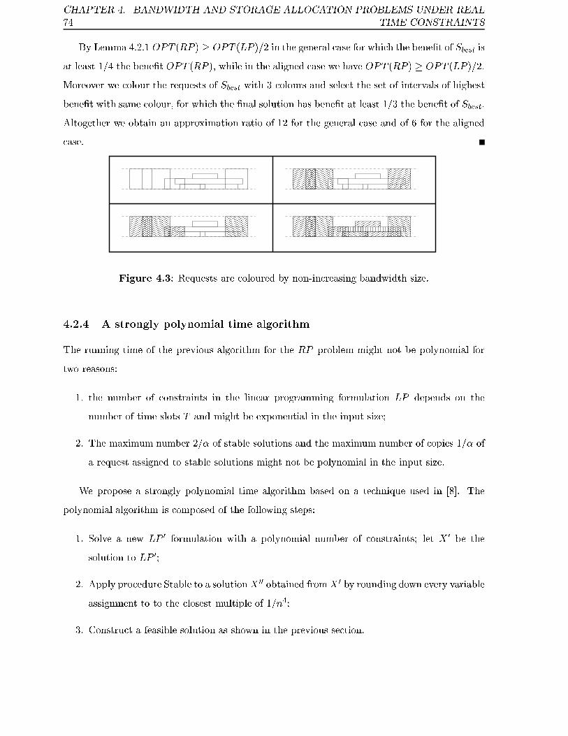
74


TIME CONSTRAINTS

By Lemma 4.2.1 OPT (RP ) � OPT (LP )=2 in the general case for which the bene�t of Sbest is

at least 1=4 the bene�t OPT (RP ), while in the aligned case we have OPT (RP ) � OPT (LP )=2.

Moreover we colour the requests of Sbest with 3 colours and select the set of intervals of highest

bene�t with same colour, for which the �nal solution has bene�t at least 1=3 the bene�t of Sbest.

Altogether we obtain an approximation ratio of 12 for the general case and of 6 for the aligned

case.

��

��

��

��

��

��

��

��

��

��

��

��

��

��

��

��

��

��

��

��

��

��

��

��

��

��

��

��

��

��

��

��

��

��

��

��

��

��

��

��

��

��

��

Figure 4.3: Requests are coloured by non-increasing bandwidth size.

4.2.4 A strongly polynomial time algorithm

The running time of the previous algorithm for the RP problem might not be polynomial for

two reasons:

1. the number of constraints in the linear programming formulation LP depends on the

number of time slots T and might be exponential in the input size;

2. The maximum number 2=� of stable solutions and the maximum number of copies 1=� of

a request assigned to stable solutions might not be polynomial in the input size.

We propose a strongly polynomial time algorithm based on a technique used in [8]. The

polynomial algorithm is composed of the following steps:

1. Solve a new LP 0 formulation with a polynomial number of constraints; let X 0 be the

solution to LP 0;

2. Apply procedure Stable to a solutionX 00 obtained fromX 0 by rounding down every variable

assignment to to the closest multiple of 1=n4;

3. Construct a feasible solution as shown in the previous section.


Since all release times, deadlines and processing times are integral we assume that each

request is processed at an integral point of time. In the LP 0 formulation they are furtherly re-

stricted to a set of integers polynomial in n, thus obtaining a number of variables and constraints

of the linear programming formulation that is polynomially bounded.

The modi�ed linear programming formulation LP 0 de�nes big slack requests and small slack

requests. A request i is big slack if di � ri > n2 � li, small slack otherwise.

A big slack request i is completely scheduled up to 1 in LP 0 for a fraction 1=n2 on each of

n2 disjoint time intervals between ri and di. The bandwidth allocated to big slack request at

any time is then bounded by 1=n.

A small slack request i may be scheduled at one of n2 + 1 time divisors between ri and di.

The distance between two divisors is less than li. The set T0, T 0

� T in the modi�ed LP 0 is the

union of all time divisors for the n requests. T 0 has cardinality O(n3).

Let OPT (LP 0) be the optimal value of the LP 0 relaxation; since at each instant the overall

bandwidth allocated for big slack requests is less than n�1 it follows that OPT (LP ) � (1 +

2n�1)OPT (LP 0).

Note that the bandwidth constraint may be satis�ed in LP 0 at two successive time divisors t1

and t2 but violated in the middle due to the overlap between a request ending at t1 and a request

starting at t2. The �rst one may actually end between t1 and t2 while the second one may start

between t1 and t2. This will lead the procedure stable to construct 3=� stable solutions to place

all the copies of the requests, rather than 2=� as shown in the previous section.

Remind that procedure Stable is applied to a solution X 00 obtained by rounding down the

optimal solution to LP 0. We will apply the following lemmas to solutionX 00 obtained by rounding

down the optimal solution to LP 0 is a fesible solution to LP 0.

Lemma 4.2.12 Given a feasible solution to LP 0 then algorithm Stable constructs at most 3�

stable solutions.

Proof: The proof is similar to the proof of Lemma 4.2.4. At most 1=� distinct copies of it need

to be placed for every request i. Since 3=� solutions are available, at least m � 2=�+1 solutions

S1; ::; Sm not containing a copy of i are available for a single replication of it. By contradiction,

if no stable solution can host the new request, then every solution has allocated at any point a

bandwidth that is at least �=2, for a total over all the solutions bigger than 1.

76


TIME CONSTRAINTS

Theorem 4.2.13 There exists a strongly polynomial algorithm for the RP problem that is 18+

O(n�1) approximated in the general case and 9 +O(n�1) approximated in the aligned case.

Proof: For the running time observe that both the number of constraints in the linear pro-

gramming formulation LP 0 and the value of � are polynomial in n; by Lemma 4.2.5 the running

time of the whole algorithm is also polynomial in n.

The proof of the approximation ratio is similar to the proof of Theorem 4.2.11. Let OPT (LP )

and OPT (LP 0) be the values of the optimal solutions to LP and LP 0 and R(LP 0) be the value

of the solution X 00 obtained by rounding down to the nearest multiple of 1=n4 every variable

assignment in solution X 0 to LP 0. Let !max be the maximum bene�t obtainable by accepting a

single request; clearly OPT (LP ) is at least !max.

Since the number of variables in LP 0 is at most n3 + n and each nonzero variable of X 0 is

rounded to the closest multiple of n�4 it follows that OPT (LP 0)�R(LP 0) � !max(n�1 + n�3)

and, therefore, for suÆciently large n,

OPT (LP 0) � R(LP 0)(1 + 2n�1):

Since OPT (LP ) � (1 + 2n�1)OPT (LP 0) we also have for a large enough n, OPT (LP ) �

R(LP 0)(1 + 5n�1).

Lemma 4.2.12 implies that the bene�t of the solution Sbest obtained by the procedure Stable

is at least R(LP 0)=3 and Lemma 4.2.1 implies that OPT (RP ) � 2OPT (LP ) in the general

case and OPT (RP ) � OPT (LP ) in the aligned case. Since we colour the requests of Sbest

with 3 colours and select the set of intervals with same colour of highest bene�t we obtain an

approximation ratio of 18 +O(n�1) for the general case and of 9 +O(n�1) for the aligned case.

4.3 A combinatorial algorithm

In this section we sketch how to replace the basic step of the approximation algorithm based

on the solution of a fractional LP formulation with a combinatorial algorithm that delivers a

constant approximation solution to the LP problem.

We partition the requests into wide requests, that ask at least 1=2 of the available bandwidth,

and narrow requests whose bandwidth requirement is less than 1=2. We solve the RP problem

4.3. A COMBINATORIAL ALGORITHM 77

separately for wide requests and narrow requests and we choose the best solution. If all requests

are wide then RP is equivalent to interval scheduling for which a 2 approximation algorithm is

known [81].

For narrow requests we replace the basic step of the algorithm based on solving the LP

formulation with a combinatorial algorithm. We divide every request in k identical requests

each one with a fraction 1=k of the bandwidth and of the pro�t of the original request. We

then apply the combinatorial algorithm of [6] for �nding an approximate integral solution to

the problem in which the only bandwidth constraint is imposed. Lemma 3.2 of [6] states the

following:

Lemma 4.3.1 For each integer k there exists a combinatorial algorithm that �nds a 2 + 1=k

approximate solution to the LP formulation if all requests are narrow.

Recall that the algorithm of section 3 can be applied to any feasible solution of the linear

programming relaxation. Therefore the combinatorial algorithm gives a solution that is away

from the optimal LP solution for at most a 2+ 1kfactor thus leading to a 12(2+ 1

k) approximate

solution for narrow requests. Combined with the 2 approximation for wide requests we obtain:

Theorem 4.3.2 For every k there exists a 26+1=k combinatorial approximation algorithm for

the RP problem.

Proof: Given k and an instance of the RP problem, the algorithm consider two problems;

the �rst one is obtained by considering only wide requests and the second one by considering

only narrow requests. We denote with OPT (RPw) and Sw the values of the optimal and of a

2 approximate solution on wide requests; analougously we denote with OPT (RPn) and Sn the

values of the optimal and of a (24 + 1=k) approximate solution for narrow requests. A(RP )

denotes the value of the solution found by the algorithm that is at least max(Sw; Sn).

Clearly the optimal solution OPT (RP ) of the given instance satis�es

OPT (RP ) � OPT (RPw) +OPT (RPn) � 2Sw + (24 +1

k)Sn:

We distinguish two cases: if Sw � Sn then

OPT (RP ) � 2Sw + (24 +1

k)Sn � (26 +

1

k)Sn � (26 +

1

k)A(RP ):

78


TIME CONSTRAINTS

If Sw > Sn then

OPT (RP ) � 2Sw + (24 +1

k)Sn � (26 +

1

k)Sw � (26 +

1

k)A(RP ):

4.4 The multiple channel case

In this section we assume that m channels, each one with a bandwidth Bj � 1, are available. For

the sake of simplicity we assume the Bj 's to be powers of 1=2. We brie y sketch the extension

of known techniques [8], to obtain a c + 1 throughput maximization approximation algorithm

for m parallel unrelated machines provided a c algorithm for a single machine. We consider

a Linear Programming formulation with variables xijt indicating the allocation of request i at

time t on machine j. We set xijt = 0 for those machines j where bi > Bj . We then solve the

LP problem and apply our rounding algorithm in order from channel 1 to channel m while we

disregard on channel j requests already accepted on a previous channel. The analysis shown in

[8] allows to conclude with the following theorem:

Theorem 4.4.1 Provided a c approximation algorithm for the RP problem on a single channel,

there exists a c+ 1 approximation algorithm for the RP problem on multiple channels.

4.5 Conclusions

In this chapter we have presented constant approximation algorithms for the RP problem, a

throughput version of bandwidth and storage allocation problems when real time constraints

are imposed. Our algorithm uses as a basis a solution of a Linear Programming formulation and

partitions it into a convex combination of integral solutions with a novel rounding technique.

We improve the approximation results found independently from our work in [6].

An interesting open problem is to study the problem in the on-line model in which requests

for bandwidth allocation are presented over time. In the on-line setting we also observe that in

reality rejection of the requests may not be allowed if enough bandwidth is available. We �nally

mention the improvement of the approximability of the problem, in particular by exploiting

some of the ideas behind the recent work by Gergov on approximating DSA [34, 35].

Chapter 5

Randomized Lower Bounds for

Online Path Coloring

In this chapter we present randomized lower bounds for on-line path coloring problems on line

and tree networks, a special class of on-line graph coloring problems. The input instance to

an online graph coloring problem is a sequence � = fv1; :::; vj�jg of vertices of a graph. The

algorithm must color the vertices of the graph following the order of the sequence. When the

color is assigned to vertex vi, the algorithm can only see the graph induced by vertices fv1; :::; vig.

The goal of a graph coloring algorithm is to use as few colors as possible under the constraint

that adjacent vertices receive di�erent colors.

Online graph coloring problems have been studied by several authors

[48, 39, 55, 85]. The study of online graph coloring has actually been started even before

the notion of competitive analysis of online algorithms was introduced [79]. Kierstead and Trot-

ter [47] in 1981 considered the online coloring problem for interval graphs. Every vertex of an

interval graph is associated with an interval of the line. Two vertices are adjacent if the two

corresponding paths s are edge-intersecting. Since interval graphs are perfect graphs [37], they

have chromatic number � equal to the maximum clique size !, i.e. the maximum number of

intervals overlapping at a single of the line.

In [47] a deterministic online algorithm that colors an interval graph of chromatic number

! with 3! � 2 colors is presented. They also prove that the 3! � 2 bound is tight: for every

deterministic algorithm there exists an input sequence where the algorithm uses at least 3!� 2

colors.

79

80 CHAPTER 5. RANDOMIZED LOWER BOUNDS FOR ONLINE PATH COLORING

The problem of coloring online an interval graph abstracts a set of scheduling problems in

wireless communication. Consider a set of requests that arrive over time. Each request speci�es

a contiguous time interval in which it has to be served. According to the FDMA technology, two

overlapping requests must use di�erent frequencies, namely two overlapping intervals (vertices

of an interval graph) must be colored with di�erent colors. The problem is on-line since the

assignment of frequencies to requests must be done upon arrival even if the requests have to be

served in the future.

The online coloring of paths on a tree network naturally gives rise to an on-line graph coloring

problem. We assume the tree network known in advance to the algorithm. Every path on the

tree network presented in the sequence is associated with a vertex of the graph. Two vertices

are adjacent in the graph if the two corresponding paths are intersecting. The graph that is

formed is called the intersection graph. This problem has recently received a growing attention

due to its application to wavelength assignment in optical networks [70, 10, 36].

An O(log n) competitive deterministic algorithm for the problem of on-line coloring paths on

a tree network has been shown by several authors (see for instance

[10, 36]). Bartal and Leonardi [10] also show an almost matching (�= log�) deterministic

lower bound on a tree of diameter � = O(logn), where n is the number of vertices of the graph.

In this dissertation we present the �rst lower bounds on the competitive ratio of randomized

algorithms for online interval graph coloring and online coloring of paths on tree networks.

Randomized algorithms for online problems [11] have often been proven to achieve competi-

tive ratios that are strictly better than deterministic online algorithms. The competitive ratio of

a randomized algorithm against an oblivious adversary is de�ned as the maximum over all the

input sequences of the ratio between the expected online cost and the optimal o�ine cost. The

input sequence for a given algorithm is generated by the oblivious adversary without knowledge

of the random choices of the algorithm. However, there is no known randomized on-line coloring

algorithm for any network topology that achieves a competitive ratio that is substantially better

than the best deterministic algorithm for the problem.

In this thesis we present the �rst randomized lower bound, up to our best knowledge, for

online coloring of interval graphs. We show that any randomized algorithm uses an expected

number of colors equal to 3! � 2 � o(1=!) for an interval graph of maximum clique size equal

to !, thus proving that randomization does not allow to substantially improve upon the best

81

deterministic algorithm of [47], answering an open question posed in [19].

Our second result is a �rst randomized (log�) lower bound for online coloring of paths on

a tree network of diameter � = O(logn). There is still a substantial gap between the presented

lower bound and the O(log n) deterministic upper bound known for the problem.

The current status of the online path coloring problem on trees can be compared with the

known results for the dual problem of selecting online a maximum number of edge-disjoint

paths on a tree network, i.e. a maximum independent set in the corresponding intersection

graph. An O(log�)-competitive randomized algorithm is possible for the online edge-disjoint

path problem on trees [2, 53], that compares with a matching (�) deterministic lower bound

obtained on a line network of diameter � = n [1]. Our result still leaves open the question if an

O(log�)-competitive randomized algorithm is possible for the online path coloring problem on

tree networks.

Our result has also implications on on-line coloring of inductive graphs. A graph is d-

inductive if the vertices of the graph can be associated with numbers 1 through n in a way that

each vertex is connected to at most d vertices with higher numbers. Irani [40] shows that any

d-inductive graph can be colored online with O(d log n) colors and presents a matching (logn)

deterministic lower bound. The graph obtained from the intersection of paths on a tree network

has been independently observed to be a (2!� 1) inductive graph by [10] and by Kleinberg and

Molloy as reported in [19]. Our lower bound for online path coloring on trees then implies a �rst

(log log n) lower bound on the competitive ratio of randomized algorithms for online coloring

of inductive graphs.

We conclude this section by mentioning the previous work on randomized online coloring

algorithms for general graphs. Vishwanathan [85] gives an O(n= log n) competitive randomized

algorithm, improving over the O(n= log� n) deterministic bound of Lov�asz, Saks and Trotter

[55]. In [85] it is also presented an ((1=(� � 1)((log n=(12(� + 1)))� 1)��1) randomized lower

bound for coloring on-line a graph of chromatic number �. However, such result is obtained for

the model in which the algorithm does not know in advance a the graph from which a subgraph

is presented. Halld�orson and Szegedy [39] give an (n= log2 n) randomized lower bound for the

problem. Bartal Fiat and Leonardi [9]�rst study the model in which the graph G from which the

vertices to color are drawn is known in advance to the online algorithm. The sequence � may

contain only a subset of the vertices of G. The algorithm must color the subgraph of G induced


by the vertices of �. The authors show that even under this model an (n�) randomized lower

bound, for a �xed � > 0, is possible.

The chapter is structured as follows. Section 5.1 presents the lower bound on online coloring

of interval graphs. Section 5.2 presents the lower bound for path coloring on tree networks.

Conclusions and open problems are in Section 5.3.

5.1 A lower bound for online interval graph coloring

In this section we present a lower bound on the competitive ratio of randomized algorithms for

online interval graph coloring.

The input instance to the online interval graph coloring problem is given by a sequence of

intervals on a line graph. Every interval is denoted by two endpoints of the line. The algorithm

must color the intervals one by one, in the order in which they appear in the sequence. The

goal is to use as few colors as possible under the constraint that any two overlapping intervals

are assigned di�erent colors.

The competitive ratio of an online algorithm for the interval graph coloring problem is given

by the maximum over all the input sequences of the ratio between the expected number of

colors used by the algorithm and the chromatic number of the interval graph, i.e. the maximum

number ! of intervals overlapping at a single point of the line.

A lower bound for randomized algorithms against an oblivious adversary is established us-

ing the application of Yao's Lemma [94] to online algorithms [19, 9]. A lower bound over the

competitive ratio of randomized algorithms is obtained by proving a lower bound on the com-

petitive ratio of deterministic online algorithms on a speci�c probability distribution over the

input sequences for the problem.

We �rst give some notation. We will denote by Pm the speci�c probability distribution

over input sequences of chromatic number ! we use to prove the lower bound. Probability

distribution Pm will be described by a set of input sequences with chromatic number m, with

every input sequence presented with equal probability.

We denote by � 2 P the generic input sequence of probability distribution P . We slightly

abuse notation by denoting with � also the set of intervals fI1; ::::; Ij�jg in the sequence.

Probability distributions P and Q are said independent if for any I1 2 �1 2 P , I2 2 �2 2 Q,

I1 and I2 are disjoint intervals. The set of sequences of probability distribution P [Q is obtained

5.1. A LOWER BOUND FOR ONLINE INTERVAL GRAPH COLORING 83

by the concatenation of every input sequence of P with every input sequence of Q.

5.1.1 The probability distribution

The probability distribution P! used for proving the lower bound is recursively de�ned. We will

resort to a pictorial help to describe the sequence.

Probability distribution P1 is formed by a single input sequence containing a single interval.

P! is the union of � independent and identical probability distributions P1!; ::::; P

�

!, as described

in Figure 5.1. The value of � will be �xed later.

Pj

! is obtained from four independent distributions P 1!�1; P

2!�1; P

3!�1; P

4!�1. The set of input

sequences of Pj

! is obtained by the concatenation of every input sequence of P 1!�1 [ P 2

!�1 [

P 3!�1 [ P 4

!�1 with every of the 10 distinct subsequences T1; ::::; T10, called con�gurations, of at

most 4 intervals described in Figure 5.2. The intervals of every of the 10 di�erent con�gurations

are numbered in Figure 5.2 following the order in which they appear in the sequence. Every

probability distribution P i!�1 is generated by applying the present de�nition for ! � 1.

Observe that every input sequence of Pm has chromatic number m. This can easily be

seen with an inductive argument. Probability distribution P1 contains a single sequence with

chromatic number 1. By induction, every input sequence from P i!�1, i = 1; ::; 4, has chromatic

number ! � 1. Every input sequence � 2 P 1!�1 [ P 2

!�1 [ P 3!�1 [ P 4

!�1 has also chromatic

number m� 1. One can check from Figure 5.2 that the concatenation of � with every of the 10

con�gurations increases the clique size and then the chromatic number by exactly 1. Since Pm

is the union of � independent probability distributions P1!; ::::; P

�

!, every sequence of Pm has

chromatic number m.

P1

m�1P2

m�1P3

m�1P4

m�1

. . . . . .

P�!

P!

P1

!

Figure 5.1: The de�nition of the probability distribution.

5.1.2 The proof of the lower bound

The proof of the lower bound is based on the following lemma:


T1

T9

T7

T5

T3

T2

T10

T8

T6

T4

I2

I3

I4

I1 I1

I4

I3

I2

I3I2I1I1

I3I2

I2

I3I1

I1

I3I2

I2I1

I1

I2

I1I2

I1

Figure 5.2: The 10 con�gurations used to form the probability distribution.

Lemma 5.1.1 Any deterministic online algorithm uses at least 3! � 2 colors with probability

at least 1� e�c on an input sequence drawn from probability distribution Pm, if � �10c

(1�e�c)4.

From the above lemma, choosing constant c large enough, say c = ln3m3, we obtain the

following Theorem:

Theorem 5.1.2 For any randomized algorithm for online interval graph coloring, there exists

an input sequence of chromatic number ! where the expected number of colors used by the

algorithm is at least 3! � 2� o(1=m).

The remaining part of this section is devoted to the proof of Lemma 5.1.1. The proof is by

induction.

The claim of Lemma 5.1.1 holds for ! = 1, since a deterministic algorithm uses one color for

the sequence from probability distribution P1 containing one single interval. Assume the claim

holds for a probability distribution P!�1, i.e. with probability at least 1� e�c, the deterministic


algorithm uses 3(! � 1) � 2 colors for an input sequence drawn from a probability distribution

Pm�1.

As an intermediate step of the proof we will prove a claim that holds for a probability

distributionPj

!, j = 1; ::; �. We denote in the following by P! the generic probability distribution

Pj

!.

Lemma 5.1.3 Consider a probability distribution P!. Assume the deterministic algorithm uses

at least 3(!� 1)� 2 colors for every input sequence �i drawn from probability distribution P i!�1,

i = 1; :::; 4. With probability at least 1=10, the deterministic algorithm uses at least 3!�2 colors

for an input sequence drawn from probability distribution P!.

Proof: Denote by Ci the set of colors used for a generic input sequence �i drawn from probability

distribution P im�1, and let Cm�1 = [

4i=1C

i. Denote by jCj the cardinality of set C. Let Cm be

the set of colors used for an input sequence from probability distribution Pm. We will prove

that jCmj � 3! � 2 with probability at least 1=10.

We distinguish four cases on the basis of the value of d = j[4i=1C

ij�(3(!�1)�2), the number

of colors exceeding 3(!� 1)� 2 used by the algorithm for the four sequences �i, i = 1; :::; 4. We

will separately consider the cases of d = 0; 1; 2 and d � 3.

d=0. In this case the deterministic algorithm uses the same set of colors for every sequence �i,

i = 1; ::; 4. The new intervals presented in any of the 10 con�gurations must be assigned

colors not inCm�1. With probability 2=5, one of con�gurations T1; T2; T3 or T4 is presented.

In all these con�gurations, one among intervals I1 and I2 contains all the intervals of �4,

the other all the intervals of �1. We further distinguish two cases: a.) Intervals I1 and I2

have assigned the same color, say c1; b.) Intervals I1 and I2 have assigned di�erent colors,

say c1 and c2.

a. With probability 1=2, the sequence is completed by intervals I3 and I4 of con�guration

T1 or T2. Interval I4 must be assigned a color di�erent from c1, say c2, since it is

overlapping interval I1. Interval I3 must be assigned a color di�erent from c1 and c2,

say c3, since it is overlapping intervals I4 and I2. Then, with probability 1=5, 3 more

colors are used, and the claim is proved.

b. With probability 1=2, the sequence is completed by interval I3 of con�guration T3 or

T4. Interval I3 is assigned a color di�erent from c1 and c2, say c3, since it overlaps


both I1 and I2. Also in this case, with probability 1=5, 3 more colors are used, thus

proving the claim.

d=1. We prove that with probability at least 1=10, 2 new colors are used by the deterministic

algorithm. Observe that a sequence �i may not use one of the colors of Cm�1 that might

be \re-used" for an interval of a con�guration Tj overlapping �i.

The following simple fact follows since a Ci contains at least jCm�1j � 1 colors:

Claim 5.1.4 For any two sequences �i; �j, i 6= j, if Ci6= Cj then Ci

[ Cj = Cm�1.

We separately consider 4 di�erent cases distinguished on the maximum cardinality s of

a subset S � f�1; �2; �3; �4g such that for every �i; �j 2 S it holds Ci = Cj. We will

separately consider the four di�erent cases, s = 1; 2; 3; 4.

s=1. In this case, every two sequences have assigned a di�erent set of colors. Then, we

have C1[ C2 = C3

[ C4 = Cm�1. With probability 1=10 con�guration T9 is given.

Interval I1 is assigned a color c1 =2 Cm�1, since for any color of Cm�1, interval I1

overlaps an interval assigned that color. For the same reason, a color c2 =2 Cm�1 is

assigned to I2. Color c2 must be distinct from c1 since interval I2 intersects interval

I1. The claim is then proved.

s=2. The case in which there are at most two sequences assigned with same set of colors

is broken in three subcases: A) �1 and �4 or �2 and �3 or �1 and �3 or �2 and �4

are assigned the same set of colors; B) Both �1 and �2 and �3 and �4 are the same

set of colors; C) �1 and �2 are assigned di�erent set of colors while �3 and �4 are

assigned the same set of colors. The symmetric of case C. is proved in an analogous

way. The 3 cases cover all the possibilities: Case A) excludes cases B) and C); If case

A) does not hold then either C1 = C2 or C3 = C4 (case C) or both C1 = C2 and

C3 = C4 (case B).

A Since s = 2, we have C16= C2 and C3

6= C4. The same argument of s=1 applies

here to prove the claim.

B) In this case we know that C1 = C26= C3 = C4. With probability 2=5, corre-

sponding to con�gurations T1, T3, T5 and T7, interval I1 includes all the intervals


of �4. Assume I1 is assigned a color c1 =2 Cm�1. With probability 1=4 con�gura-

tion T7 is given. For every color of C2[C3 = Cm�1, interval I2 of con�guration

T7 overlaps an interval assigned with that color. Since interval I2 intersects I1,

it is assigned a color c2 =2 Cm�1 distinct from c1, then proving the claim.

Otherwise, consider the case in which interval I1 of con�guration T1, T3, T5 or

T7 is assigned a color of Cm�1, say co1. With probability 1=2, corresponding to

con�gurations T1 and T3, interval I2 includes sequence �1. Consider the case in

which I2 is assigned a color c1 =2 Cm�1. With probability 1=2, corresponding to

the selection of con�guration T3, interval I3 overlaps all the intervals of �2 and

�3. For every color of C2[C3 = Cm�1, interval I3 overlaps an interval assigned

with that color. I3 also intersects interval I2 assigned with a color c1 =2 Cm�1.

Interval I3 is then assigned a color c2 =2 Cm�1 thus proving the claim.

We are left to consider the case of I1 and I2 assigned with a color of Cm�1, say

co1 and co2. With probability 1=2, corresponding to con�guration T1, interval I3

includes sequence �2 and interval I4 includes sequence �3. Since C1 = C2 and

C3 = C4, we have C2[ co2 = Cm�1 and C

3[ co1 = Cm�1. Interval I3 that overlaps

�2 and intersects interval I2, must be assigned a color c1 =2 Cm�1. Interval I4,

that includes sequence �3, and intersects interval I1 and I3, must be assigned a

color c2 =2 Cm�1 distinct from c1. The claim is then proved.

C.) In this case C16= C2 and C3 = C4. Thus, from Claim 5.1.4, C1

[ C2 = C!�1.

Since s = 2, C16= C3 and C2

6= C3. With probability 2=5, con�guration T1, T3,

T5 or T7 is given, and interval I1 that includes sequence �4 is presented. Consider

the case in which interval I1 is assigned a color c1 =2 Cm�1. With probability 1=4,

corresponding to con�guration T7, interval I2, that includes �1, �2 and �3, is

presented. For any color of Cm�1, I2 includes an interval assigned with that

color. I2 also intersects interval I1 assigned with color c1. I2 is thus assigned a

color c2 =2 Cm�1 di�erent from c1, thus proving the claim.

We �nally consider the case of I1 assigned with a color co1 2 Cm�1. With prob-

ability 1=4 con�guration T5 is presented. Interval I2 overlaps sequences �1 and

�2. Since C1[ C2 = Cm�1, I2 is assigned a new color, say c1. Since C

3 = C4,

C3[co1 = Cm�1. Interval I3 overlaps all the intervals of �

3, I1 assigned with color


c01 and I2 assigned with color c1. Interval I3 is then assigned a color c2 =2 Cm�1,

thus proving the claim.

s=3 We have two symmetric cases, either C3 = C4 or C1 = C2. If C3 = C4, we have

that either C1 = C3 or C2 = C3, but C16= C2. Under these assumptions, the

same argument used in case C.) of s=2 allows to prove the claim. Case C1 = C2 is

analogous.

s=4 In case C1 = C2 = C3 = C4, all the sequences are assigned the same set of colors.

The same analysis of case d = 0 allows to prove the claim.

d=2. In this case jCm�1j = 3m � 3. To prove the claim, a new color must be used with

probability at least 1=10. With probability 1=10, con�guration T10 is presented. For any

color of Cm�1, interval I1 overlaps an interval assigned with that color. I1 is thus assigned

a new color c1 =2 Cm�1.

d�3. In this case jCm�1j � 3m� 2, the claim is then proved.

We �nally present the proof of Lemma 5.1.1. Let p(m) be the probability that a deterministic

algorithm uses 3m� 2 colors on an input sequence from probability distribution Pm. Consider

a probability distribution Pj

m formed by the union of probability distributions P i

m�1, i = 1; ::; 4.

By induction, we assume that the algorithm uses at least 3(m � 1) � 2 colors with probability

p(m� 1) � (1� e�c) on an input sequence �i drawn from probability distribution P im�1.

With probability p(m�1)4, a deterministic algorithm uses at least 3(m�1)�2 colors for all

the input sequences �i drawn from probability distributions P im�1, i = 1; ::; 4. With probability

p(m � 1)4 we are then under the assumptions of Lemma 5.1.3. We then obtain from Lemma

5.1.3 that with probability at least 110p(m� 1)4, the algorithm uses at least 3m� 2 colors for an

input sequence from Pj

m, j = 1; ::; �.

Since all the Pj

m that form Pm are mutually independent, the probability that a determin-

istic algorithm uses less than 3m � 2 colors on all the input sequences drawn from probability

distributions Pj

m is then upper bounded by

�1�

1

10p(m� 1)4

��

�1�

1

10(1� e�c)4

�� e��

(1�e�c)4

10 :

5.2. A LOWER BOUND FOR ONLINE PATH COLORING ON TREES 89

If � � 10c(1�e�c)4

, the given expression has value less than e�c.

We have then proved that with probability at least (1� e�c), a deterministic algorithm uses

at least 3m�2 colors for a sequence from a probability distribution Pm, thus implying the claim

of Lemma 5.1.1.

5.2 A lower bound for online path coloring on trees

We prove that any randomized algorithm for online path coloring on trees of diameter � =

O(log n) has competitive ratio (log�).

We establish the lower bound using Yao's Lemma [94]. We prove a lower bound on the

competitive ratio of any deterministic algorithm for a given probability distribution on the

input sequences for the problem.

The tree network we use for generating the input sequence is a complete binary tree of L � 4

levels. The root of the tree is at level 0, the leaves of the tree are at level L� 1. The 2l vertices

of level l are denoted by rlj, j = 0; :::; 2l � 1. The direct ancestor of vertex u is denoted by p(u).

We will indicate by [a; b] the path in the tree from vertex a to vertex b.

The input sequence for the lower bound is generated in � = (logL) stages. We will prove

that at stage i = 0; ::; ��1, with high probability, the number of colors used by any deterministic

algorithm is i. An optimal algorithm is shown to be able to color all the paths of the sequence

with only 2 colors, thus proving the lower bound.

At stage i of the input sequence, we concentrate on a speci�c level li = li�1 � d(3i log 16� +

log(16(��i) log n))e�1 of the tree, with l0 = L�1. It turns out that at least (16�)3i

16(��i) log n

vertices of level li�1 are contained in each subtree rooted at a vertex of level li. To simplify

notation, the jth vertex of level li, rlij, is denoted by ri

j.

We de�ne at stage i a set of pairs Ii = f(uij; vi

j); j = 0; :::; 2li �1g, where ui

j; vi

jare two leaves

of the subtree rooted at vertex rijof level li.

Set I0 = f(r0j; r0j); j = 1; :::; 2L � 1g is composed by one degenerated pair for every leaf of

the tree.

Set Ii is formed by selecting at random for every vertex rij, two distinct pairs of Ii�1 in the

subtree rooted at rij. The pair associated with vertex ri

j, in the following often denoted by pair

rij, is formed by the two second vertices of the two selected pairs. More formally:


1. For every vertex rijof level li, j = 0; :::; 2li � 1:

Select uniformly at random two distinct vertices ri�1k1j

; ri�1k2j

of level li�1 in the subtree

rooted at vertex rij. Let (ui�1

k1j

; vi�1k1j

); (ui�1k2j

; vi�1k2j

) 2 Ii�1 be the two pairs associated

with vertices ri�1k1j

and ri�1k2j

.

2. Ii = f(vi�1k1j

; vi�1k2j

) : j = 0; :::; 2li � 1g is the set of pairs at stage i.

The input sequence at stage i is formed for every pair rijof Ii, by a path from the �rst vertex

of the pair to the direct ancestor of vertex rij:

Pi = f[uij; p(ri

j)] : j = 0; :::; 2li � 1g.

We prove in the following that any optimal algorithm serves the input sequence with two

colors. We �rst observe:

Lemma 5.2.1 Every edge of the tree is included in at most two paths of [i�0Pi.

Proof: For every vertex rij, for every stage i, denote by Ei

jthe set of edges in the subtree rooted

at rijwith both endpoints of level between li�1 � 1 and li, plus the edge (r

ij; p(ri

j)). (For a leaf

vertex r0j, E0

jincludes only the edge (r0

j; p(r0

j))). We separately prove the claim for every set of

edges Eij.

Edges of Eijare not included in any path Pi0 , i

0 < i. Every leaf vertex is the endpoint of at

most one path in the sequence and one path from P0. By the construction of the input sequence,

vertices uijand vi

jare the only leaf vertices in the subtree rooted at ri

jthat may be endpoints

of paths in a set Ii0 , i0� i. The claim is then proved.

The following lemma bounds the size of the optimal solution.

Lemma 5.2.2 The optimal number of colors for any input instance from the probability distri-

bution is 2.

Proof: We show a two coloring of an input instance with: (i.) Every path directed from a leaf

to an ancestor of the leaf; (ii.) Every edge of the tree included in at most two paths. We proceed

from the top to the bottom of the tree. Consider an internal vertex v (initially the root), and

let v1 and v2 be the two children of v. Consider edge (v1; v). (A similar argument holds for

edge (v2; v)). If no path of the input sequence includes both (v1; v) and (v; p(v)) (assume this


is the case if v is the root), edge (v1; v) is crossed by at most 2 paths, say p1 and p2, that end

at v. Paths p1 and p2 are assigned the two available colors. If only one path, say p1, includes

both (v1; v) and (v; p(v)), there is at most one path, say p2, including edge (v1; v) that ends at

v. Path p2 is assigned the color not given to p1. If there are two paths, p1 and p2, including

both (v1; v) and (v; p(v)), these have already been colored. The coloring procedure then moves

to consider vertex v1.

In the remainder of the section we show that the expected number of colors used by any

deterministic online algorithm is (logL), thus implying the lower bound.

The following lemma will be used to prove our result.

Lemma 5.2.3 For each pair (uij; vi

j) 2 Ii, path [vi

j; p(ri

j)] intersects a single path in every set

Pj, j � i.

Proof: We prove the claim by induction on the number of stages. The claim is true for pairs

of I0. Path [vij; p(ri

j)] is formed by the union of paths [vi�1

k2j

; p(ri�1k2j

)] and [p(ri�1k2j

); p(rij)].

If the claim holds at stage i� 1, path [vi�1k2j

; p(ri�1k2j

)] intersects one single path for every Pj ,

j � i� 1.

Path [p(ri�1k2j

); p(rij)] includes only edges of level lower than li�1 � 1. Since no path of a set

Pj , j � i� 1, includes edges of level lower than li�1 � 1, path [uij; p(ri

j)] can intersect only path

[uij; p(ri

j)] 2 Pi on edge (ri

j; p(ri

j)). This is also the single path of Pi in the subtree rooted at

vertex rij, thus showing the claim.

We introduce some more notation. Given a pair (uij; vi

j) 2 Ii, let C

ij= fc0; ::::; cig be a set

of i+ 1 colors, where cj is the color assigned to the single path of Pj intersecting [vij; p(ri

j)].

Pair (uij; vi

j) is a good pair if Ci

jis formed by i + 1 distinct colors. We will prove that with

high probability, for any stage i = 0; ::; �, there exists at least one good pair of level i. The

existence of a good pair of level i gives the evidence that at least i+1 colors have been used by

the deterministic algorithm, thus proving the claim.

We also denote by ON the number of colors used by the online deterministic algorithm on

a speci�c input sequence drawn from the probability distribution. Xijis a boolean variable

denoting the event that rijis a good pair.

The following claim gives us a suÆcient condition for a pair of level li to be a good pair.


Lemma 5.2.4 Pair (uij; vi

j) 2 Ii of level i is a good pair if it is obtained from selecting two good

pairs (ui�1k1j

; vi�1k1j

), (ui�1k2j

; vi�1k2j

) with Ci�1k1j

= Ci�1k2j

.

Proof: For every color c 2 Ci�1k1j

= Ci�1k2j

, by Lemma 5.2.3, path [vi�1k1j

; p(ri�1k1j

)] and [vi�1k2j

; p(ri�1k2j

)]

intersect a single path assigned with color c. Path [uij; p(ri

j)] that contains [vi�1

k1j

; p(ri�1k1j

)] is then

assigned with a color ci =2 Ci�1k1j

. Path [vij; p(ri

j)] intersects path [ui

j; p(ri

j)] assigned with color ci

on edge (rij; p(ri

j)). Pair (ui

j; vi

j) is then a good pair with set of colors Ci

j= Ci�1

k2j

[ fcig.

Let ni = (16�)3i

16(� � i) log n be the number of vertices of level li in a subtree rooted at a

vertex of level li+1. Let fi =P

jXijbe the number of good pairs of level li in a subtree rooted at

a vertex of level li+1. Let pi+1 be a value such that let Pr[Xi+1j

jON � � \ fi � nipi=2] � pi+1,

namely a lower bound on the probability of a pair ri+1j

of level li+1 to be a good pair when the

algorithm uses at most � colors along the sequence and there are at least nipi=2 good pairs of

level li in the subtree rooted at vertex ri+1j

.

The next Lemma assigns a value to pi.

Lemma 5.2.5 For a pair ri+1j

of level li+1, Pr[Xi+1j

jON � �\fi � nipi=2] � pi+1 =�

116�

�3i+1.

Proof: We prove the claim by induction. The claim holds for level l0 since pair r0jis

associated with a single color. Assume by induction it holds for level li. For the proof of the

claim we denote i1 = (uik1j

; vik1j

) and i2 = (uik2j

; vik2j

) the two pairs of Ii selected at random in the

subtree rooted at ri+1j

and by Ci

k1j

and Ci

k2j

the two set of colors associated with the two pairs.

In the following we shorten notation by indicating X1 = Xii1, X2 = Xi

i2,C1 = Ci

k1j

, C2 = Ci

k2j

.

By Lemma 5.2.4, we can derive the following equality for the probability of a pair of level

li+1 to be a good pair:

Pr[Xi+1j

jON � � \ fi � nipi=2] = Pr[X1 \X2 \ C1 = C2jON � � \ fi � nipi=2]

Since we are conditioned to those input sequences for which ON � �, every pair of level li is

associated with at most �!(��i)!i!

� �i di�erent set of colors. Let C � �i be the number of distinct

set of colors assigned to the good pairs of level i. To estimate a value for pi+1, we consider the

ratio between the cardinality of the set of positive events and the cardinality of the total set of

events in the random selection of two pairs at step 1 of the probability distribution. We compute

the probability of having a good event conditioned to the existence of at least nipi=2 good pairs


of level li in the subtree rooted at a vertex ri+1j

. The cardinality of the set of positive events is

minimized when the good pairs are equally distributed among the C color classes. We therefore

obtain:

Pr[X1 \X2 \C1 = C2jON � � \ fi � nipi] � Cbmpi

2Cc � b

mpi

2C� 1c

m(m� 1)

� C

�mpi

2C� 1

��mpi

2C� 2

�m(m� 1)

� Cmpi

4Cmpi

4C

m2

=1

16Cp2i

We then apply the inductive hypothesis to obtain

Pr[Xi+1j

jON � � \ fi � nipi=2] �1

16�i

�1

16�

�23i

=

�1

16�

�i+23i

�

�1

16�

�3i+1;

therefore proving the claim.

The claim of the next Lemma is a statement of sharp concentration around the expectation

of the number of good pairs at every stage of the probability distribution.

Lemma 5.2.6 Pr[fi � nipi=2jON � �] � 1� 1n2(��i)�1

:

Proof: We prove the claim by induction. The claim holds for a level l0 since the single pair of

level l0 is a good pair. Assume Claim 5.2.5 for level li+1 and Claim 5.2.6 for level li. We then

prove Claim 5.2.6 for level li+1.

To give a statement of sharp concentration around the expectation of function fi =P

jXij

we should consider that random variables Xj 's are not necessarily independent since the deter-

ministic algorithm may coordinate the coloring of paths in di�erent subtrees. Therefore, we can

use Cherno�-Hoe�ding bounds only if we make additional assumptions on the coloring produced

by the deterministic algorithm until stage i.

Consider all vertices ri+1j

in a subtree rooted at a vertex of level li+2. We restrict our

attention to those input sequences I for which the number of good pairs of level li in a subtree


rooted at every vertex ri+1j

is xj � nipi=2, j = 1; :::; ni+1. By the induction hypotesis, the total

probability of the sequences in I is at least pI ��1� 1

n2(��i)�1

�n�

�1� 1

n2(��i�1)

�.

We prove the claim of sharp concentration for every subset of I that produced the same input

sequence up to stage i. Within every such subset, variables Xi+1j

are independent, for which we

can safely apply Cherno�-Hoe�ding bounds to estimate Pr[fi+1 � ni+1pi+1=2jON � �]. By the

theorem of total probability, this implies the claim for the whole set I.

We apply the following version of Cherno�-Hoe�ding bounds: Let fi+1 =P

j Xi+1j

and let

� =P

j Pr[Xi+1j

= 1]. For every Æ > 0,

Pr[fi+1 < (1� Æ)�] < e(��Æ2=2):

By the inductive hypothesis given by Lemma 5.2.5, a lower bound over the expected number

of good pairs at level li+1 under condition fi � nipi=2, is given by � � � = ni+1pi+1 =�116�

�3i(16�)3

i16(�� i�1) log n = 16(�� i�1) log n. The following expression is easily obtained

from the expression of Cherno�'s bounds:

Pr[fi+1 < (1� Æ)�] � Pr[fi+1 < (1� Æ)�] < e(��Æ2=2)

� e(��Æ2=2):

Setting Æ = 1=2 we obtain:

Pr[fi+1 < ni+1pi+1=2] < exp(�2(�� 1� 1) log n) =1

n2(��i�1):

We therefore have for the probability of sharp concentration:

Pr[fi+1 � ni+1pi+1=2jON � �] � pI Pr[fi+1 � ni+1pi+1=2]

�

�1�

1

n2(��i�1)

�2� 1�

1

n2(��i�1)�1;

thus proving the claim.

The construction of the input sequence is repeated until stage i = � � 1 such that jIij =

2li � (16�)3i16(� � i) log n. Easy computation shows � = (logL). Lemma 5.2.6 shows that

under these assumptions with probability at least (1 � 1n), there exist a large number of good

pairs of level l��1. Then, with probability at least (1 � 1n), a set of � distinct colors is used by

the deterministic algorithm under the condition that ON � �. We therefore obtain:

5.3. CONCLUSIONS 95

E[ON ] � E[ON jON > �] Pr[ON > �] +E[ON jON � �] Pr[ON � �]

� �Pr[ON > �] + �(1�1

n) Pr[ON � �]

� �=2;

where the last inequality follows since n > 2. Lemma 5.2.2 states that the optimal solution

uses two colors on any of these input sequences. Thus, the lower bound over the competitive

ratio of randomized algorithms is given by �=4. We then conclude with the following theorem:

Theorem 5.2.7 There exists a (log�) lower bound on the competitive ratio of randomized

algorithms for online path coloring on a tree of diameter � = O(logn).

5.3 Conclusions

In this chapter we have presented the �rst randomized lower bounds for online interval graph

coloring and online path coloring on tree networks. This line of research is aimed to establish if

there exists a speci�c network topology where randomized online algorithms obtain substantially

better competitive ratios than deterministic algorithms.

A �rst open problem is to close the gap between the randomized lower bound for online path

coloring on trees and the best deterministic upper bound known for the problem.

The lower bound for path coloring on trees is actually obtained on a 2-colorable graph. This

does not preclude the existence of an algorithm that uses �+ O(log�) colors for the problem.

A second open problem, posed in [19], is to establish a multiplicative lower bound rather than

an additive lower bound, i.e. a lower bound on a graph of arbitrary large chromatic number.

Chapter 6

System Architecture for Location

Based Services

CDPD [30] has been deployed in North America for providing data services for mobile users. In

this chapter, we present a system architecture whose purpose is extracting location information

of a CDPD subscriber from the handheld device and making it available to a location server.

The location server can then be accessed by an Internet Service Provider (ISP) in order to

o�er suitable location based services. For example, location information can be exploited by

Yahoo yellow pages to o�er the closest emergency services to the mobile users. The localization

technique we implemented, i.e. the BSIC localization method, allows us to identify the location

of a user within the range of a cell. The main idea of this method is that through a suitable

protocol, the MSCI protocol, we can obtain from the modem the Base Station Identi�cation

Code (BSIC), namely a number that unambiguously identi�es the antenna to which the user is

currently connected. Since an antenna covers a speci�c region (i.e a cell), the BSIC also identi�es

the cell in which the mobile user is currently located. This technique su�ers from an inherent

lack of accuracy, since the dimensions of a cell has a range that goes from some meters to some

kilometers. We discuss methods for improving accuracy that are based on analyzing information

obtained from multiple cells and using readily available system parameters like received signal

strength indicator (RSSI), block error rates (BLER) etc. Furthermore we compare and contrast

the accuracy �gures of these techniques with those of a global positioning system (GPS) in

order to determine the applicability of the di�erent localization techniques. For example, in

a metropolitan area the use of a CDPD based localization technique can be suÆcient to the

97

98 CHAPTER 6. SYSTEM ARCHITECTURE FOR LOCATION BASED SERVICES

purposes of general directory services. However, if a user wants to be routed to a speci�c point

of interest a GPS is needed since the accuracy derived from a CDPD system is not suÆcient.

We stress that we investigate a handset assisted solution to localize a subscriber. This approach,

in contrast to network oriented localization solutions, has a minimal impact on the telecom-

munication network and protects privacy (the user has to explicitly disclose his localization

information).

The rest of the chapter is organized as follows. In section 6.1 we describe the current localization

techniques and their main features. In section 6.2 we introduce the CDPD architecture, namely

the wireless environment in which we developed our localization method. Section 6.3 describes

the Modem Status Con�guration Interface (MSCI) protocol and the BSIC localization method,

while section 6.4 presents a system architecture that allows to map the BSIC into geographic

coordinates, namely latitude and longitude. Finally we show how these coordinates can be

exploited by Service Providers to o�er location based services. In section 6.5 we evaluate the

quality of the accuracy of the BSIC localization method, and we compare it to the the GPS

accuracy. Finally section 6.6.2 presents two methods, the multiple cells method and the RSSI

measurement method, in order to improve the accuracy of the BSIC localization method.

6.1 Localization Technology

The ability to locate the position of a mobile device is crucial for providing geographically speci�c

value-added information, and it has been indicated in a recent study [56] as a key factor for the

development of new wireless application.

Applications using mobile location service technologies include eet management, vehicle

tracking for security, tracking for recovery in event of theft, telemetry, emergency services,

location identi�cation, navigation, location based information services and location based ad-

vertising. The largest push for localization technology is coming from the US. There, mobile

telephone operators have been forced by the FCC to provide emergency 911 services by October

2001 in such a way that the location of the caller could be determined within a radius of 125

meters in 67% of all cases. There are three major localization techniques [83]:

� Triangulation can be done via lateration, which uses multiple distance measurements be-

tween known points, or via angulation, which measures angle or bearing relative to points

with known separation;

6.1. LOCALIZATION TECHNOLOGY 99

� Proximity measures nearness to a known set of points;

� Scene analysis examines a view from a particular vantage point, such as antennae or mobile

terminals.

Implementation of location systems generally uses one or more of these techniques to locate

objects and/or people. Furthermore location systems can be either terminal based or network

based. In terminal based systems, it is the mobile device itself that determines the location.

Normally these systems are less accurate but they do not require signi�cant network upgrade.

Network based systems provide more accurate localization information, but require a signi�cant

network upgrade. In the following we summarize the main features of the current localization

techniques, see [43, 56] for further details.

� GPS GPS (Global Positioning System) is a system that consists of 24 satellites circling the

earth in a particular constellation to each other so that several satellites fall within line of

sight for any GPS receiver on Earth. Because the satellites are continuously broadcasting

their own position and direction, the GPS receiver can calculate its position with an

excellent approximation. Anybody can use the GPS system for free with an appropriate

receiver. GPS has been developed in the US for military use, but from the beginning of the

decade it has been usable (with lower resolution) for civilian purposes. GPS technology

for mobile phones is being currently developed for example by SnapTrack and SiRF and

it is already used in Benefon dual mode GSM/GPS handsets.

� TOA This method uses the Time Of Arrival (TOA) of signals between the mobile phone

and the cellular antenna. TOA is used to capture time di�erence of arrival information

to make calculations to determine an estimate of the mobile terminal position. This

technology requires large network modi�cations and is therefore not cost-e�ective. Rolling

out TOA for an entire network is estimated to cost as much as 10 times the price of an

E-OTD system.

� E-OTD The E-OTD (Enhanced Observed Time Di�erence) system works by using the

existing GSM infrastructure to determine the mobile phones location. When a user calls

selected service providers, E-OTD simultaneously sends data indicating the phones posi-

tion. It works by comparing the relative times of arrival, at the handset and at a nearby

�xed receiver, of signals transmitted by the underlying mobile network base stations. The


E-OTD system overlays the existing mobile network. Suppliers for E-OTD solutions in-

clude CPS, Ericsson and BT Cellnet.

� COO COO (Cell Of Origin) can be used as a location �xing scheme for existing customers

of network operators, but it is not as exact as the other methods. It requires no modi�ca-

tion to the mobile terminal, but normally the network operator has to do some signi�cant

upgrade work. In urban areas COO might be suÆcient to determine location fairly accu-

rately, because the cell size is very small. In rural areas, where the cell radius is larger,

it might not be enough accurate. The solution we present in this work is based on this

approach, but as we will see, it does not require any signi�cant network upgrade.

6.2 CDPD Architecture

The CDPD architecture consists of two essential entities shown in Figure 6.1, the mobile end

station (MS) and the network. A user accesses CDPD network using a Mobile end System

(MS) that establishes a connection to a Mobile Data Base Station (MDBS) on a speci�c radio

channel. The MDBS is responsible for providing the data link for the set of radio channels serving

a cell, i.e. the geographic area covered by a MDBS. A MDBS is controlled by a single Mobile

Data Intermediate System (MDIS). MDISs are networked with other MDISs and �xed networks

through routing and relay elements known as Intermediate Systems (IS) that are unaware of

mobility.

The CDPD forum has speci�ed standards for implementing a Location Service [30]. However,

all proposals are network oriented and heavily impact on the network traÆc because of location

requests. In the following we present our solution, the BSIC localization method. We exploit the

ability of a MS to get location information from the modem, without requiring any signi�cant

network upgrade.

When a CDPD user is connected to a MDBS, the modem is continuously updated with the

information on which cell tower the MS is currently connected to. In particular each cell, is

identi�ed by a unique number, the Base Station Identi�cation Code (BSIC). The MS can get

information on the current BSIC from the modem through the Modem Status Con�guration

Interface (MSCI) protocol ( see section 6.3). Finally, the BSIC can be mapped into geographical

coordinates as appropriate for the provision of location-based services.

6.3. THE MSCI PROTOCOL 101

MDBS

MDBSMDBS

MD-IS

MDBS

MD-IS

IS

IS

IS

MDBS

MD-IS

MS

MS

Cellular Provider X Cellular Provider Y

Cellular Provider Z

MDBS

MDBSMDBS

MD-IS

MDBS

MD-IS

IS

IS

IS

MDBS

MD-IS

MS

MS

MDBS

MDBSMDBS

MD-IS

MDBS

MD-IS

IS

IS

IS

MDBS

MD-IS

MS

MS

Cellular Provider X Cellular Provider Y

Cellular Provider Z

Figure 6.1: CDPD Architecture

For the purposes of a demonstrator, a Compaq handheld Pocket PC (HP3600) was used equipped

with a CDPD Novatel Wireless modem MSCI enabled [91], and AT&T Wireless was used as

the service provider. Note that for all practical purposes, any modem can be interrogated via

the standard serial interface using AT commands. This may however require additional device

drivers to be written to enable simultaneous status request and maintain a TCP connection.

The MSCI protocol alleviates this requirement.

6.3 The MSCI Protocol

MSCI (Modem Status Con�guration Interface) is a protocol which allows the modem param-

eters to be con�gured and monitored using UDP packets over a data connection. The MSCI

Communication model is based on the client-server paradigm (see Figure 6.2). The client sends

a datagram to the server, specifying the function the MSCI Server has to perform and possibly

some arguments, and waits for the answer (see Figure 6.3). The MSCI Server is implemented in

the Novatel wireless modem and it is identi�ed by the private non-routable IP address 10.0.0.1

on port 4950(see [91] for further details). Therefore the MSCI Server runs on the same handset in

which the Novatel wireless modem is installed. Three di�erent kinds of functions are supported

by the MSCI protocol:


Figure 6.2: The MSCI Communication Model.

Function Code Arguments

1 octet n octets

MSCI CLIENT MSCI SEVER

0x03 Arguments

0x02


1 octet n octets


1 octet n octets

MSCI CLIENTMSCI CLIENT MSCI SEVERMSCI SEVER

0x03 Arguments

0x02

Figure 6.3: Client/Server Messages.

� Status information: it allows to gather information on the status of the modem. For

example we can obtain the signal strength indicator (RSSI), the BSIC or the block error

rate (BLER);

� Con�guration information: it allows to gather information on the modem con�guration.

For example we can verify if the modem is con�gured to detect some speci�c events;

� Commands: it allows to send command to the modem. For example we can properly set

the modem registers.

As we have seen in section 6.2 the BSIC unambiguously identi�es a cell, hence knowing the

current BSIC, namely the BSIC of the base station to which the user is currently connected, we

can estimate with some approximation (see Table 6.2) the location of a user. The current BSIC

can be gathered invoking the Status Request Function (Function Code 0x02). This function is

used by the MSCI client to request the modem status information to the MSCI Server; observe

that no arguments are required. The MSCI Server responds with a Status Response (Function

Code 0x03). In table 6.1 we show the arguments of the Status Response function. We just

consider those �elds that we will use to implement our localization methods. The CDPD Status

�eld indicates if the channel is acquired and/or the link is stablished and/or the CDPD device is

registered. Current Channel indicates the channel that is currently used for the communication

between the wireless devices and the antenna. Current RSSI indicates the current signal strength

and �nally Current Cell Site ID is the BSIC.

6.4. THE GEOPROXY ARCHITECTURE 103

Field Octets Description

CDPD Status 1 Mask containing 3 bits

0x01: TRUE if channel acquired

0x02: TRUE if link established

0x04: TRUE if registered

Link Status 1 Contains same information as bit 0x02

in the CDPD Status �eld

Last Registration Error 1 (Block ID 0x40, Parm ID 0x11)

RRM State 1 (Block ID 0x40, Parm ID 0x18)

Current Area Color Code 1 (Block ID 0x40, Parm ID 0x16)

Current Channel 2 MSB �rst (Similar Block ID 0x40, Parm ID 0x14)

Current RSSI 1 (Block ID 0x40, Parm ID 0x12)

Current BLER 1 (Block ID 0x40, Parm ID 0x13)

Reserved 1

Current Power Level 1 (Block ID 0x40, Parm ID 0x19)

Current Service ID 3*2 MSB �rst (Similar Block ID 0x40, ParmID 0x17)

SPI: 0-65535

WASI: 0-65535

SPNI: 0-65535

Current Cell Site ID (BSIC) 2 MSB �rst (Similar Block ID 0x40, Parm ID 0x15)

Current Power Product 1 (Block ID 0x40, Parm ID 0x1a)

Table 6.1: Arguments of the Status Response function

6.4 The GEOPROXY Architecture

The BSIC can be e�ectively used to estimate the approximate location of a MS. The ability to

localize a user just depends on a successful connection to a cell tower.

It remains to explain how this information can be exploited by a service provider. We need

a further component that is capable of communicating to a service provider the approximate

location in a suitable format, possibly latitude and longitude (BSIC could be meaningless).

This is the main goal of the Geoproxy architecture. The overall architecture consists of 5 main

components:

� Browser: the user accesses the localization service by a Browser; it may be Netscape or

Internet Explorer.

� GEOPROXY: A Web server that maps BSIC into geographical coordinates, namely lati-


tude and longitude. The mapping function could have been implemented inside the MS,

without requiring an HTTP connection. Nevertheless we implemented the HTTP based

solution for two main reasons: 1) The BSIC label could change over time, 2) Such a so-

lution allows us to send back a customized HTML page to the user (see step 6 in �gure

6.4).

� LOCALPROXY: is a local daemon, running on the mobile user device, that acts as an

MSCI Client. The Localproxy gets the current BSIC from the modem and it is also

responsible for communicating the BSIC to the GEOPROXY. When a user wants to

access a localization service, he has to connect by the browser to the Localproxy (just by

typing the URL http://localhost:4444).

� The MSCI Server. Recall that the MSCI Server runs on the same MS in which is installed

the Novatel wireless modem.

� Content/Service Provider: it exploits the user geographical coordinates to provide location

based services.

Figure 6.4: The Architecture

In what follows and in Figure 6.4 we outline a description of the procedures to ful�ll a new

request for a location based service:

6.5. ACCURACY 105

1. A user wants to access a location based service. He connects by browser to the LOCAL-

PROXY at the URL http://localhost:4444;

2. LOCALPROXY acts as a MSCI Client. It sends a Status Request to the MSCI Server;

3. The MSCI Server answers by the Status Response function. LOCAL PROXY gets the

BSIC from the arguments of the Status Response;

4. LOCALPROXY sends the BSIC to the GEOPROXY using the HTTP GET

(e.g. http://<GEOPROXY>?BSIC=<BSIC> );

5. GEOPROXY maps the<BSIC> into geographical coordinates <geo coo>, namely latitude

and longitude of the base station;

6. GEOPROXY sends back to the LOCALPROXY the Localized Service Page, an HTML

page with links to the Content/Service Provider; each link provides the <geo coo> to a

Content/Service Provider through an HTTP GET;

7. LOCALPROXY redirects the incoming HTML page to the Browser which displays the

Localization Service Page to the user;

8. The user clicks on a link and connects to a Content/Service Provider;

9. The Content/Service Provider processes the <geo coo> and provides the required service.

6.5 Accuracy

BSIC localization method can be used to provide the approximate location of a user; the main

advantages of this technique is that it is easy to implement, it does not require signi�cant network

upgrade and it is relatively fast in detecting the BSIC and subsequently perform a translation

of the BSIC into geographic coordinates. The main disadvantage, is the lack of accuracy; the

dimension of a cell vary from some meters to some kilometers (see Table 6.2).

In some cases and for some applications that accuracy could be considered insuÆcient. For

this reason, in the next sections we try to better evaluate the accuracy of the BSIC localization

method, and we compare it with the GPS, at present the best location technology. Finally, we

experiment two methods to improve the BSIC localization method.


Cell type Antenna location Cell Dimension (km)

Large macrocell Above rooftop level 3-30

Small macrocell Above rooftop level 1-3

Microcell Below or about rooftop level 0.1-1

Picocell Below rooftop level 0.01-1

Nanocell Below rooftop level 0.01-0.001

Table 6.2: Di�erent Cell Types

6.5.1 GPS measurement

Using the GPS it is possible to accurately measure the position of a MS. Although the GPS

su�ers from some inaccuracy, (accuracy mainly depends on the number of satellites visible in

a particular location) it is normally limited within 10 meters; hence, it is much more accurate

than localization techniques based on cell site boundaries. For this reason, in what follows we

refer to the GPS position being the actual location of the mobile user.

To compare the performances of the localization technique based on the BSIC with respect to

the GPS, we modi�ed the LOCALPROXY to record every 2 seconds all modem information,

namely CDPD status, Received Signal Strength Indication (RSSI), Block Error Rate (BLER),

power level and BSIC. Furthermore, for each record in the log, we append the GPS information

, namely location coordinates, accuracy (estimated horizontal/vertical position error in meters),

velocity and a time stamp. It may happen that some records in the log �le miss the modem

information and/or the GPS information. This is mainly due to insuÆcient channel availability

for CDPD connections or to shadow e�ects in the presence of obstacles (buildings or trees)

preventing a GPS connection. In the following we denote by Total Samples the overall number

of records in the log �le, while we denote by Useful Samples the number of records in the log

�le for which we have both GPS and modem information. Finally, we denote by NO GPS the

number of records in the log �le for which we do not have GPS information or it is useless and

we denote by NO modem the number of records in the log �le for which we do not have modem

information or it is useless (see Figure 6.7). The analysis of the log �les allows us to compare

the BSIC method with the GPS. In Figure 6.5 we give a pictorial representation of some data

in the log �les obtained while driving about New York. Each point in the map represents a

location obtained through the GPS. Di�erent colors of the points correspond to di�erent BSICs.

6.5. ACCURACY 107

Figure 6.5: A NY BSCI/GPS map Figure 6.6: A zoom of the NY map

The isolated points in the map, namely the points that are not part of the path, represent the

location of the MDBS. Zooming the map (see Figure 6.6) one can see that sometimes the path

is not continuous, this is due to lack of GPS connection.

6.5.2 Average distance

A �rst measure to estimate the quality of the BSIC localization method is the computation of

the average distance of the position of a MS with respect to the correspondent MDBS.

Namely if the log �le contains N Useful Samples, and we denote by d(MDBS(i); GPS(i))

the distance between the MDBS (identi�ed by the BSIC in the log �le) and the MS (the exact

location of the MS is obtained through the GPS) of the ith sample, the average distance is

de�ned as �d = 1N

PN

i=1 d(MDBS(i); GPS(i)).

As we have seen in the previous sections, the BSIC localization method su�ers from an

inherent inaccuracy. We can identify the region in which a MS is located, but not its actual

position. Hence, using this localization method, we implicitly assume the likely location of a

MS to be the location of the MDBS . Thus a small �d, with a relatively small variance, gives

the evidence that the MDBS location can well approximate the MS actual location in most of

the cases. However, a large average distance and/or a large variance can lead to non signi�cant

�gures.

We ran the experiment in three di�erent contexts, an urban context (NY metropolitan area), a

sub-urban context (Madison, NJ-Morris Town, NJ) and �nally on a highway context (driving


URBAN.

0

0.2

0.4

0.6

0.8

1

1.2

1.4

1.6

1.8

2

samples

Km

SUBURBAN.

0

0.2

0.4

0.6

0.8

1

1.2

1.4

1.6

1.8

samples

Km

HIGWAY.

0

1

2

3

4

5

6

7

8

9

samples

Km

URBAN SUBURBAN HIGWAY

Total Samples 2237 665 1188

Useful Samples 1840 378 520

�d 0.79Km 0.49Km 2.91Km

Stand. Deviation 0.39Km 0.38Km 2.00Km

Min. 0.02Km 0.11Km 0.95Km

Max. 1.85Km 1.70Km 8.35Km

No GPS 136 0 68

No modem 261 287 600

Figure 6.7: Average distance experiments.

from NY to Madison, NJ ).

The results of the experiments are shown in �gure 6.7 . In the table Min is the minimum

distance of a MS to the corresponding MDBS, namelymin(d(MDBS(i); GPS(i)));8i, Max is the

maximum distance of a MS to the corresponding MDBS, namelymax(d(MDBS(i); GPS(i)));8i.

In the urban area most of the time we have both CDPD and GPS data available (Useful

Samples are about 82% of the Total Samples). The average distance is about 800 meters.

The standard deviation is about 50% of the average distance and about 21% of the maximum

distance. In the suburban area, the average distance (about 500 meters) is even smaller than in

NY samples, but the number of useful samples decreases signi�cantly (about 56% of the Total

Samples). Furthermore the number of useless CDPD samples is a big fraction of the total.

The standard deviation is about 77% of the average distance (the value are more spread with

respect to the urban case) and about 22% of the maximum distance. Finally in the highway, the

average distance is very high, about 3 kilometers. This can be explained with the presence of

big areas without obstacles in the middle between the MT and the MDBS; furthermore higway

cell size is bigger than urban cell size. The useful samples are about 44% of Total Samples and

6.5. ACCURACY 109

the standard deviation is about 69% of the average distance and about 24% of the maximum

distance. Finally observe that the coverage of the CDPD network is better in urban area (only

about 12% of the total samples have useless modem information, while in suburban and higway

areas is about 50%), while the GPS coverage is better in suburban and higway areas (this is

mainly because of the presence of high buildings in the urban area).

6.5.3 Service Accuracy

For speci�c contexts, even a poor quality in accuracy of location method can be suÆciently

reliable to o�er suitable services to the users. An average distance of 2 Kms can be considered

inappropriate in an urban context, but it may be suÆcient in a highway context. For this reason

we introduce the notion of service accuracy. Suppose to know both the MS's actual position,

denoted by GPS, and the BSIC of the cell tower to which the MS is connected, denoted by

BSIC. Denote by SGPS;d

, the set of providers of service S within d Km to GPS and by SBSIC;d

,

the set of providers of service S within d Km to BSIC. The service accuracy A� is a function

of the service S, the distance d, BSIC and GPS, de�ned as follows:

A�(S; d;BSIC;GPS) = jSBSIC;d

\SGPS;d

SGPS;d

j

If we call \good service" the services that are close to user actual location, namely SGPS;d

,

this function counts the fraction of \good services" that we can locate using the BSIC as an

approximate location of the user.

An alternative measure of accuracy can be the fraction of \approximate services", namely

the fraction of services in SBSIC;d

that are also good services. Thus we introduce the following

alternative de�nition of accuracy. The service accuracy A�� is a function of the service S, the

distance d, BSIC and GPS, de�ned as follows:

A��(S; d;BSIC;GPS) = jSBSIC;d

\SGPS;d

SBSIC;d

j

Both measures provide acceptable and complementary estimations of service accuracy and we

refer to both in this work. If a user wants to know which are the closest cafeterias with respect

to his location, a service accuracy close to one means that there are no signi�cant di�erences

between the BSIC localization method and the GPS. Nevertheless, if the user wants to know

how to get to those cafeterias, the GPS may become essential. Moreover, a good \cafeterias"

accuracy does not necessarily imply a good accuracy for other services. In fact, service accuracy


Figure 6.8: Yahoo yellow pages. Figure 6.9: Service Accuracy.

mainly depends on the di�erence between the distribution of speci�c services around the MDBS

and around the actual MS location.

In the following we present some experiments on service accuracy. In Figure 6.9 we have collected

the samples driving on Avenue of the Americas (NY) approximately between Bleecker St. and

24 St., while the CDPD modem was continuously connected to the cell tower located at latitude

40.733 and longitude -73.999 (BSIC 28857 ). The average distance of these samples is about

0:63Km, suÆciently close to the average distance found in the urban area experiment, see Figure

6.7, to consider this set of samples representative of the urban context. We limit our attention

to the samples A,B,C,D. Points A and D are located at the end point of the path, far away

from the cell tower, thus they possibly represent a bound to the service accuracy. Point B is

the closest point with respect to the cell tower. Point C has a distance (0.77Km) very close to

the average urban distance (0.79Km), hence it can be considered as \the average sample" (see

Figure 6.7 and Table 6.3).

In order to determine the set of providers Sx;d that allow us to calculate the service accuracy,

we connect to Yahoo yellow pages as follows:

http://yp.yahoo.com/py/ypResults.py?stx=starbucks&city=New+York&state=NY&

country=us&slt=40.733&sln=-73.999,

where stx is the service provider (Starbucks), slt is x's latitude and sln is x's longitude. The

result are the Starbucks cafeterias close to location x (see Figure 6.8).

6.5. ACCURACY 111

latitude longitude Distance to the Cell Tower (Km)

A 40.729359 -74.002235 0.49

B 40.733372 -73.999657 0.07

C 40.739378 -73.995312 0.77

D 40.743443 -73.992378 1.29

Table 6.3: Distances.

S=Starbucks

BSIC=28857

d

GPS 4.82 Km 3.22 Km 1.6 Kma 0.8 Km

A 80% 80% 84.6% 62.5%

B 100% 100% 100% 100%

C 80% 90% 92.3% 50%

D 65% 65% 53.8% 12.5%

Figure 6.10: Starbucks Accuracy (A�)

a1 mile

S=Starbucks

BSIC=28857

d

GPS 4.82 Km 3.22 Km 1.6 Kma 0.8 Km

A 80% 80% 91.6% 83.3%

B 100% 100% 100% 100%

C 80% 90% 60% 57.1%

D 65% 65% 35% 11.1%

Figure 6.11: Starbucks Accuracy (A��)

a1 mile

In Figures 6.10 and 6.11 we show the result of the service accuracy calculation for di�erent

values of the distance d.

First observe that the �gures of both A� and A�� are very close. Service accuracy is greater

than 50% independently from the distance d, except for the farthest point D. In particular point

C, that represents the average sample, has a service accuracy greater than 50% with d = 0:8

Km. We can conclude that in most cases, half of the Starbucks cafeterias that are considered

close using the MS actual position (GPS location) can be considered close also using the BSIC

localization method. Observe that point B, being so close to the Cell Tower, has a service

accuracy of 100% all the times. Moreover, in almost all cases service accuracy increases with

the distance d, but this is not always true. For example if we consider point C (see Figure 6.10),

service accuracy is 90% if d is 3:22 Km and decrease to 80% when d is 4:82 Km. This can be

explained with the distribution of the Starbucks cafeteria around the MDBS and around point

C that strongly in uences the accuracy values.

In Figures 6.12 and 6.13 we evaluate the service accuracy of Barnes & Noble bookshops.


S=Barnes & Noble

BSIC=28857

d

GPS 4.82 Km 3.22 Km 1.6 Kma 0.8 Km

A 92% 80% 100% 25%

B 100% 100% 100% 100%

C 92% 100% 100% 75%

D 92% 100% 100% 75%

Figure 6.12: Barnes & Noble Accuracy (A�)

a1 mile

S=Barnes & Noble

BSIC=28857

d

GPS 4.82 Km 3.22 Km 1.6 Kma 0.8 Km

A 100% 100% 83.3% 100%

B 100% 100% 100% 100%

C 100% 90.9% 83.3% 75%

D 92.3% 90.9% 83.3% 75%

Figure 6.13: Barnes & Noble Accuracy (A��)

a1 mile

Also in this case the �gures of both A� and A�� are very close and service accuracy is

considerably high in each point also for small values of d. The only exception is the small value

of service accuracy of point A when d is 0:8 Km (see Figure 6.12) . This can be explained with

a relatively high concentration of Barnes & Noble bookshops north of the cell tower.

We did not extend the evaluation of service accuracy in suburban area, or in the highway, since

in these contexts the di�usion of speci�c service providers like Starbucks or Barnes & Noble

is considerably smaller. This means that a query like \which are the closest Barnes & Noble

bookshops" may probably have as an answer that the closest bookshop is within ten kilometers.

With such big distances there are no signi�cant di�erences between BSIC location method and

GPS, unless the question is \How to get to the closest Barnes & Noble bookshop".

6.6 Techniques to improve BSIC method accuracy

6.6.1 Accuracy improvement using multiple cells

The BSIC method allow us to state that the MS is somewhere inside a speci�c region covered

by a cell, however it is not even possible to determine if the user is located north or south of

the MDBS. We simplify and consider the region covered by a cell to be a circle having the

center in the MDBS and a �xed radius (from some meters - nanocells, to some kilometers -

large macrocell, see Table 6.2). By using multiple cells one can greatly enhance the accuracy of

localization. The main idea is as follows: if a MS can connect to multiple cells, this means that

the user is in a region covered by all these cells (assuming overlapping cell boundaries). In what

follows we discuss in more detail the algorithm used for the multiple cells localization method.

6.6. TECHNIQUES TO IMPROVE BSIC METHOD ACCURACY 113

The MSCI protocol allows us to specify the Channel List (CL), the list of channels to be

used for a CDPD connection. If the modem is con�gured to work in the Use Channel List mode

(see MSCI protocol Block ID 0x00 Parm ID 0x05) the connection is established only to those

channels speci�ed in the CL. Each MDBS has a set of channels that can be used to establish a

CDPD connection. The CL allows us to explore this set of channels identifying all the MDBSs

around a MS. The algorithm, is shown in Figure 6.14

1. Set Set use CL mode

2. Set CL = all channels

3. While CL is not empty

4. Start connection

5. The modem connects to MDBS identi�ed by BSIC using channel C

6. Delete C from CL

7. End While

Figure 6.14: The Algorithm

Since each MDBS M uses only a speci�c set of channels S, when at step 6 we delete all the

elements of S from CL, we avoid the reconnection to M. Hence the next possible connection

at step 4 will be to another MDBS or possibly to nobody else. Running this algorithm, and

possibly exploring the whole CL, we can identify all the MDBSs \visible" to a MS.

Figure 6.15: A multiple cells experiment

InTable 6.4 we show the results of an experiment on multiple cells localization method. The


Round BSIC MDBS Location Channel

1 33487 C 674

2 33489 C 677

3 33489 C 667

4 6044 Unknown Location 724

5 6044 Unknown Location 725

6 31406 A 685

7 31406 A 681

Table 6.4: Running the algorithm

MS is located in B (see Figure 6.15), and runs the algorithm. During the �rst three connections

the MS connects to a MDBS located in C (NOTE: BSICs 33487, 33488 , 33489 correspond to

the same location). At this moment we can only assert that the MS is somewhere in the C

region. The �fth and sixth connections are to a cell tower of which we do not know the location.

Finally the last two connections are to the BSIC 31406 corresponding to location A. Since the

MS was able to connect to both the cell towers A and C, we can conclude that it is somewhere

in the region covered by both of them.

Although this method can be considered as an improvement of the BSIC method, it has sev-

eral disadvantages. The algorithm is extremely slow. Performances can be improved by knowing

the association between channels and cells in advance, in this way step 6 of the algorithm could

delete, in just one step, all channels associated to a particular MDBS, avoiding the reconnection

to the same cell more than once. Furthermore if the algorithm connects to just one cell, this

does not necessarily mean that this is the only cell visible by the user. In fact it may happen

that the connection is not allowed due to traÆc congestion. Finally, any insertion/deletion from

the CL requires a shutdown and restart of the modem, and consequently any data ow would

be interrupted. Anyway we think that most of these problems can be addressed by simple

improvements of the MSCI protocol.

6.6.2 Accuracy improvement using RSSI

RSSI measurements can be exploited to improve accuracy of location [90]. Several methods have

been studied to estimate the distance through RSSI [52], but all of them su�er from inaccuracy

6.6. TECHNIQUES TO IMPROVE BSIC METHOD ACCURACY 115

- 12 0

- 10 0

-8 0

-6 0

-4 0

-2 0

0

sa mple s

RS

SI

c b a b c

- 12 0

- 10 0

-8 0

-6 0

-4 0

-2 0

0

sa mple s

RS

SI

c b a b c

Figure 6.16: RSSI measurement driving on route A

due to the di�erences in terrain attenuation. The main problem is that the same value of RSSI

can correspond to dramatically di�erent distances due to the presence of obstacles between the

MS and the MDBS. Jean-Marc Latapy in [50] proposes a new model to determine the distance,

based on the construction of the RSSI interval map. This map identi�es the regions around a

MDBS with values of the RSSI in the same interval. In other words as an isobaric map shows

same pressure layers, and can be used to identify areas with speci�c pressure levels, an RSSI

interval map shows layers with the same RSSI. If we know the value R of the current RSSI,

and the RSSI interval map around the MDBS, then we can identify the interval in the map

containing R, and thus we can better estimate the region in which the MS is located.

The experiments in Figures 6.16 and 6.17 show how to build a simple RSSI map of the region

shown in Figure 6.18.

-12 0

-10 0

-8 0

-6 0

-4 0

-2 0

0

samp les

RS

SI

a b c

-12 0

-10 0

-8 0

-6 0

-4 0

-2 0

0

samp les

RS

SI

a b c

Figure 6.17: RSSI measurement driving on route B


Figure 6.18: Building an RSSI interval map.

Driving on route A, we obtain the values of RSSI 1 showed in Figure 6.16. The peak of the

RSSI (i.e. the lowest RSSI in dB), approximately corresponds to the closest location to the cell

tower. We can identify at least three RSSI intervals (a:[-40db,-60dB],b:[-60dB,-80dB],c:[-80dB,

-120dB]). Using this map we can assert that if a user is connected to the base station MDBS,

and measures an RSSI lower than �60dB (region a), then he/her is reasonably close to the

MDBS, on the contrary if the RSSI is in the region c, then he/her is fairly distant from the

MDBS. Driving on route B we obtain the values of RSSI showed in Figure 6.17. In this case

is not possible to identify an RSSI peak, and furthermore the �gure shows an almost constant

behavior for the �rst half of the samples (region a). So the improvements in accuracy that can

be achieved through RSSI measurements are less accurate than in the previous case (the region

a is too large). The experiment in Figure 6.19 shows the RSSI map while moving along the NJ

transit railway from Hudson Essex (the train left from NY Penn Station) to Maplewood. The

regions a,b,c,d, correspond to points in which the MT is connected to a speci�c cell. Observe

that the RSSI behavior is almost a stair function in proximity of the cell region while it is

more jagged in the boundary region except where no connection is available (�113dB). This

behavior allows us to better localize a user. If we consider region c, we can easily de�ne two

further regions, approximately corresponding to values of RSSI of �77dB and �94dB. Thus for

example, if we know a commuter being connected to the cell tower covering region c, and the

RSSI being close to one of the above values, we can easily assert whether the train is closer to

1The values of the RSSI can be easily gathered through the MSCI protocol, using the Status Request function

6.7. CONCLUSIONS AND FUTURE WORKS 117

Figure 6.19: RSSI measurements on the railroad.

region b or to region d. Furthermore, between the �77dB region and �94dB region, there is

a narrow discontinuity (RSSI = �113dB) that can be used to detect when the train transits

from one region to the other.

6.7 Conclusions and Future Works

In this chapter we have presented a system architecture whose purpose is extracting location

information of CDPD subscribers from a wireless device and making it available to a location

server. Moreover we have discussed the accuracy of this location technique and we have imple-

mented some other techniques to improve such accuracy. The main objective of the future work

will be the implementation of a similar solution in the GSM environment. We are implement-

ing an extension of the PPP protocol that allows us to interact with any modem (not being

restricted to MSCI enabled modem). We are also exploring the location potentialities o�ered by

the SIMToolkit. The SIMToolkit is a tool to program the mobile SIM phone in order to provide

new customized services.

Bibliography

[1] B. Awerbuch, Y. Azar, and S. Plotkin. Throughput-competitive online routing. In Pro-

ceedings of the IEEE Symposium on Foundations of Computer Science, pages 32{40, 1993.

[2] B. Awerbuch, R. Gawlick, T. Leighton, and Y. Rabani. On-line admission control and

circuit routing for high performance computing and communication. In Proceedings of the

35th Annual IEEE Symposium on Foundations of Computer Science, pages 412{423, 1994.

[3] K.R. Baker. Introduction to sequencing and scheduling. Wiley, 1975.

[4] Hari Balakrishnan, Venkata N. Padmanabhan, Srinivasan Seshan, and Randy H. Katz. A

comparison of mechanisms for improving TCP performance over wireless links. IEEE/ACM

Transactions on Networking, 5(6):756{769, 1997.

[5] Nicholas Bambos. Toward power-sensitive network architectures in wireless communica-

tions: concepts, issues, and design aspects. IEEE Personal Communications, 5(3):50{59,

June 1998.

[6] Amotz Bar-Noy, Reuven Bar-Yehuda, Ari Freund, Joseph (SeÆ) Naor, and Baruch Schieber.

A uni�ed approach to approximating resource allocation and scheduling. In Proceedings

of the Thirty-Second Annual ACM Symposium on the Theory of Computing, Las Vegas,

Nevada, 2000.

[7] Amotz Bar-Noy, Ran Canetti, Shay Kutten, Yishay Mansour, and Baruch Schieber. Band-

width allocation with preemption. In Proceedings of the Twenty-Seventh Annual ACM

Symposium on the Theory of Computing, pages 616{625, Las Vegas, Nevada, 29 May{1

June 1995.

119

120 BIBLIOGRAPHY

[8] Amotz Bar-Noy, Sudipto Guha, Joseph (SeÆ) Naor, and Baruch Schieber. Approximating

the throughput of multiple machines under real-time scheduling. In Proceedings of the

thirty-�rst annual ACM symposium on Theory of computing, pages 622{631, Atlanta, GA

USA, 1{4 May 1999.

[9] Y. Bartal, A. Fiat, and S. Leonardi. Lower bounds for on-line graph problems with appli-

cation to on-line circuit and optical routing. In Proceedings of the 28th ACM Symposium

on Theory of Computing, pages 531{540, 1996.

[10] Y. Bartal and S. Leonardi. On-line routing in all-optical networks. In Proceedings of

the 24th International Colloqium on Automata, Languages and Programming, LNCS 1256,

pages 516{526. Springer-Verlag, 1997.

[11] S. Ben-David, A. Borodin, R.M. Karp, G. Tardos, and A. Widgerson. On the power of

randomization in on-line algorithms. In Proceedings of the 22nd Annual ACM Symposium

on Theory of Computing, 1990.

[12] Paul Bender, Peter Black, Matthew Grob, Roberto Padovani, Nagabhushana Sind-

hushayana, and Andrew Viterbi. CDMA/HDR; A bandwith-eÆcient high-speed wireless

data service for nomadic users. IEEE Communications Magazine, 38(7):70{77, July 2000.

[13] Y. Bernet. A framework for integrated services operation over di�serv networks. Internet

Draft, May 2000.

[14] C. Berrou and A. Glavieux. Near optimum error correcting coding and decoding: turbo-

codes. IEEE Transactions on Communications , 44(10):1261 {1271, October 1996.

[15] G. Bianch and N. Blefari-Melazzi. Grip: Qos support over stateless di�serv networks

by means of localized measurements and decisions. Lecture Notes on Computer Science,

Springer-Verlag, 1989, 1989.

[16] G. Bianchi and N. Blefari-Melazzi. A migration path to provide end-to-end qos over stateless

networks by means of a probing-driven admission control. Internet Draft, March 2001.

[17] S. Blade, D. Black, M. Carlson, E. Davies, Z. Wang, and W. Weiss. An architecture for

di�erentiated services. RFC2475, December 1998.

BIBLIOGRAPHY 121

[18] Helmut Bolcskei, A. Paulraj, K V S. Hari, Rohit U Nabar, and Willie W. Lu. Fixed

Broadband Wireless Access: State of the Art, Challenges and Future Directions. IEEE

Communications Magazine, 39(1):100{108, January 2001.

[19] A. Borodin and R. El-Yaniv. Online Computation and Competitive Analysis. Cambridge

University Press, 1998.

[20] R. Braden, L Zhang, S. Berson, S. Herzog, and S. Jamin. Resource re servation protocol

(rsvp) - version 1 functional speci�cation. RFC2205, September 1997.

[21] L. Breslau, S. Jamin, and S. Schenker. Comments on the performance of measurement-based

admission control algorithms. IEEE INFOCOM 2000, March 2000.

[22] L. Breslau, E. W. Knightly, S. Schenker, I. Stoica, and H. Zhang. Endpoint admission

control: Architectural issues and performance. ACM SIGCOMM 2000, August 2000.

[23] A. De Carolis. Qos-aware handover support in mobile ip: Secondary home agents. IETF-

DRAFT.

[24] Justin Chuang and Nelson Sollenberger. Beyond 3G: Wideband data access based on OFDM

and dynamic packet assignment. IEEE Communications Magazine, 38(7):78{87, July 2000.

[25] J M. CioÆ, G P. Dudevoir, M V. Eyuboglu, and G D. Forney. MMSE decision-feedback

equalizers and coding: Parts I & II. IEEE Transactions on Communications, 43(10):2582{

2604, Oct. 1995.

[26] P. Conforto, C. Tocci, G. Losquadro, F. Fedi, R.E. Sheri�, and A. Vitaletti. Suited/gmbs

system: Architecture and mobile terminal. IST Mobile Communication Summit 2001,

September 2001.

[27] Thomas M. Cover and Joy A. Thomas. Elements of Information Theory. John Wiley and

Sons, Inc., New York, 1991.

[28] J.Wein D.Karger, C.Stein. Scheduling algorithms. Algorithms and Theory of Computation

Handbook, CRC Press, 1999.

[29] http://www.estec.esa.nl/artes3/projects/12telbios/telbios.htm.

[30] CDPD Forum. Cellular digital packet data system speci�cation, release 1.1. January 1995.

122 BIBLIOGRAPHY

[31] Juan A. Garay, Inder S. Gopal, and Shay Kutten. EÆcient on-line call control algorithms.

Journal of Algorithms, 23(1):180{194, April 1997.

[32] M. R. Garey and D. S. Johnson. Computers and Intractability { A Guide to the Theory of

NP-Completeness. Freeman, San Francisco, 1979.

[33] Michael R. Garey and David S. Johnson. Computers and intractability : a guide to the

theory of NP-completeness. W H. Freeman., San Francisco, 1979.

[34] Jordan Gergov. Approximation algorithms for dynamic storage allocation. In European

Symposium on Algorithms (ESA'96), volume 1136 of Lecture Notes in Computer Science,

pages 52{61. Springer, 1996.

[35] Jordan Gergov. Algorithms for compile-time memory optimization. In Proc. of the 10th

ACM-SIAM Symposium on Discrete Algorithms, pages 907{908, 1999.

[36] O. Gerstel, G.H. Sasaki, and R. Ramaswami. Dynamic channel assignment for WDM

optical networks with little or no wavelength conversion. In Proceedings of the 34th Allerton

Conference on Communication, Control, and Computing, 1996.

[37] M. Golumbic. Algorithmic Graph Theory and Perfect Graphs. Academic Press, New York,

NY, 1980.

[38] M. Grossglauser and D. N. C. Tse. A time-scale decomposition approach to measurement-

based admission control. IEEE INFOCOM 1999, March 1999.

[39] M.M. Halld�orsson and M. Szegedi. Lower bounds for on-line graph coloring. In Proceedings

of the 2nd Annual ACM-SIAM Symposium on Discrete Algorithms, pages 211{216, 1992.

[40] S. Irani. Coloring inductive graphs on-line. In Proceedings of the of 31th Annual IEEE

Symposium on Foudations of Computer Science, pages 470{479, 1990.

[41] http://www.ist-suited.com/.

[42] General aspects of quality of service and network performance in digital networks, including

isdns. ITU-T Recomm. I.350, March 93.

[43] G Borriello J. Hightower. Location systems for ubiquitos computing. Computer, IEEE

Computer Society, 34(8):57{66, August 2001.

BIBLIOGRAPHY 123

[44] Niranjan Joshi, Srinivas R. Kadaba, Sarvar Patel, and Ganapathy Sundaram. Downlink

scheduling in CDMA data networks. In ACM MobiCom, pages 179{190, 2000.

[45] B. Kalyanasundaram and K.Pruhs. Speed is as powerful as clairvoyance. In IEEE Sympo-

sium on Foundations of Computer Sci., pages 214{221, 1995.

[46] H. A. Kierstead. A polynomial time approximation algorithm for dynamic storage alloca-

tion. Disccrete Mathematics, 88:231{237, 1991.

[47] H. A. Kierstead and W. T. Trotter. An extremal problem in recursive combinatorics.

Congressus Numerantium, 33:143{153, 1981.

[48] H. A. Kierstead and W. T. Trotter. On-line graph coloring. In Lyle A. McGeoch and

Daniel D. Sleator, editors, On-line Algorithms, volume 7 of DIMACS Series in Discrete

Mathematics and Theoretical Computer Science, pages 85{92. AMS/ACM, February 1991.

[49] D.E. Knuth. The Art of Computer Programming, Vol. 1: Fundamental Algorithms, 2nd

Edition. Addison-Wesley, 1973.

[50] Jean-Marc Latapy. Gsm mobile station locating. PhD thesis, Norwegian University of

Science and Technology, 1996.

[51] L.Becchetti, S.Diggavi, S.Leonardi, A. Marchetti-Spaccamela, S. Muthukrishnan,

T. Nandagopal, and A. Vitaletti. Scheduling algorithms for next generation multirate

wireless networks. AT&T Labs Research Report, Jan 2001.

[52] William C. Y. Lee. Mobile Communications Engineering. McGraw-Hill Telecommunica-

tions, 2 edition, 1998.

[53] S. Leonardi, A. Marchetti-Spaccamela, A. Presciutti, and A. Ros�en. On-line randomized

call-control revisited. In Proceedings of the 9th ACM-SIAM Symposium on Discrete Algo-

rithms, pages 323{332, 1998.

[54] S. Leonardi and A. Vitaletti. Randomized lower bounds for online path coloring. RAN-

DOM 98: International Workshop on Randomization and Approximation Techniques in

Computer Science, Barcelona, Spain, pages 232{247, October 1998. Preliminarly accepted

to Information and Computation.

124 BIBLIOGRAPHY

[55] L. Lov�asz, M. Saks, and W.T. Trotter. An on-line graph coloring algorithm with sublinear

performance ratio. Discrete Mathematics, 75:319{325, 1989.

[56] Durlacher Research Ltd. Mobile commerce report, 1998.

[57] Yuming Lu and R W. Brodersen. Integrating power control, error correction coding,

and scheduling for a CDMA downlink system. IEEE Selected Areas in Communications,

17(5):978{989, May 1999.

[58] David G. Luenberger. Linear and Non-linear programming. Addison-Wesley, Reading,

Mass., 2nd edition, 1984.

[59] V. Marziale and A. Vitaletti. A framework for internet qos requirements de�nition and eval-

uation: an experimental approach. IST Mobile Communication Summit 2001, September

2001.

[60] S.Muthukrishnan M.Bender, S.Chakrabarti. Flow and stretch metrics for scheduling con-

tinuous job streams. Proceedings of Annual Symposium on Discrete Algorithms (SODA

'98), pages 270{279, 1998.

[61] C.Murta M.Crovella, M.Harchol-Balter. Task Assignment in a Distributed System: Im-

proving Performance by Unbalancing Load. Technical Report 97-018, Boston University,

1997.

[62] M.Harchol-Balter M.Crovella, R.Frangioso. Connection Scheduling in Web Servers. Tech-

nical Report 99-003, Boston University, 1999.

[63] Sanjiv Nanda, Krishna Balachandran, and Sarath Kumar. Adaptation techniques in wireless

packet data services. IEEE Communications Magazine, 38(1):54{65, January 2000.

[64] K. Nichols, S. Blake, F. Baker, and D. Black. De�nitions of the di�erentiated service �eld

(ds �eld) in the ipv4 and ipv6 headers. RFC2474, December 1998.

[65] E. Perkins. Ip mobility support. RFC2002, October 1996.

[66] E. Perkins. Mobile ip. Communications Magazine, pages 84{99, May 1997.

[67] Ampl: A modeling language for mathematical programming. http://www.ampl.com.

BIBLIOGRAPHY 125

[68] Loqo optimization toolkit, 2000. http://www.orfe.princeton.edu/ loqo.

[69] S. Muthukrishnan R. Jana, T. Johnson and A. Vitaletti. Location based services in a

wireless wan using cellular digital packet data (cdpd). MOBIDE 2001: Second ACM inter-

national workshop on Data engineering for wireless and mobile access, Santa Barbara, CA

USA, May 2001.

[70] P. Raghavan and E. Upfal. EÆcient routing in all-optical networks. In Proceedings of the

26th Annual ACM Symposium on Theory of Computing, pages 133{143, 1994.

[71] Theodore S. Rappaport. Wireless Communications, Principles & Practice. Prentice Hall,

Inc., Piscataway, New Jersey, 1996.

[72] R.Jana, T.Johnson, S.Muthukrishnan, and A. Vitaletti. System and method for enabling

data-mode location aware mobile services. United States provisional patent application.

[73] R.Jana, T.Johnson, S.Muthukrishnan, and A. Vitaletti. System and method for enabling

handset-based network enhanced location services. United States provisional patent appli-

cation.

[74] R.Jana, T.Johnson, S.Muthukrishnan, and A. Vitaletti. System and method for handset-

assisted, location tracking with multiple servers and services. United States provisional

patent application.

[75] A. Marchetti-Spaccamela S. Leonardi and A. Vitaletti. Approximation algorithms for band-

width and storage allocation problems under real time constraints. FST TCS 2000: Foun-

dations of Software Technology and Theoretical Computer Science 20th Conference, New

Delhi, India, pages 409{420, December 2000. Submitted to Journal of Algorithms.

[76] S.Muthukrishnan S.Acharya. Scheduling on-demand broadcasts for heterogenous: new met-

rics and algorithms. ACM Mobicom, pages 43{54, 1998.

[77] Prasun Sinha, Narayanan Venkitaraman, Raghupathy Sivakumar, , and Vaduvur Bhargha-

van. WTCP: A Reliable Transport Protocol for Wireless Wide-Area Networks. In ACM

MobiCom, pages 231{241, 1999.

[78] D. Sleator and R.E. Tarjan. Amortized EÆciency of List Update and Paging Rules. Com-

munications of ACM, 28:202{208, 1985.

126 BIBLIOGRAPHY

[79] D. Sleator and R.E. Tarjan. Amortized eÆciency of list update and paging rules. Commu-

nications of ACM, 28:202{208, 1985.

[80] M. Slusarek. A coloring algorithm for interval graphs. In Proc. of the 14th Mathematical

Foundations of Computer Science, pages 471{480, 1989.

[81] F.C.R. Spieksma. On the approximability of an interval scheduling problem. Journal of

Scheduling, 2:215{2227, 1999.

[82] Thomas J. J. Starr and John CioÆ. Understanding digital subscriber line technology. Pren-

tice Hall, Inc., Upper Saddle River, New Jersey, 1999.

[83] www.cs.washington.edu/research/portolano/papers/UW-CSE-01-07-01.pdf.

[84] V.Bharghavan T.Nandagopal, S.Lu. A uni�ed architecture for the design and evaluation of

wireless fair queueing algorithms. ACM Mobicom, pages 132{142, 1999.

[85] S. Vishwanathan. Randomized on-line graph coloring. Journal of Algorithms, 13:657{669,

1992.

[86] Andrew J. Viterbi. CDMA : principles of spread spectrum communication. Addison-Wesley

Pub. Co., Reading, Mass., 1995.

[87] W.Almesberger, T.Ferrari, and J. Y. Le Boudec. Srp: a scalable resource reservation

protocol for the internet. IWQoS'98, May 1998.

[88] Ellen Kayata Wesel. Wireless multimedia communications : networking video, voice, and

data. Addison-Wesley, Inc., Reading, Mass., 1998.

[89] P. P. White. Rsvp and integrated services in the internet: a tutorial. IEEE Communications

magazine, 35(5), May 1997.

[90] Svein Yngvar Willassen. A method for implementing Mobile Station Location in GSM. PhD

thesis, Norwegian University of Science and Technology, 1998.

[91] NOVATELL WIRELESS. Notes on the modem sta-

tus / con�guration interface protocol, v1.8, March 2000.

http://www.novatelwireless.com/support/download/MSCI Protocol.pdf.

BIBLIOGRAPHY 127

[92] J. Wroclawski and A. Charny. Integrated service mapping for di�erentiated services net-

works. Internet Draft, March 2000.

[93] J: Wroclawsky. The use of rsvp with ietf integrated services. RFC2210, September 1997.

[94] A. Yao. Probabilistic computations: Towards a uni�ed measure of complexity. In Pro-

ceedings of the 17th Annual IEEE Symposium on Foundations of Computer Science, pages

222{227, 1977.

La Dottora Ricer in Ingegneria Inf orma tica XIV Ciclodottoratoii/media/students/... ·...

Documents

Transcript of La Dottora Ricer in Ingegneria Inf orma tica XIV Ciclodottoratoii/media/students/... ·...