L5 Polynomial / Spline Curves - GitHub Pages
33
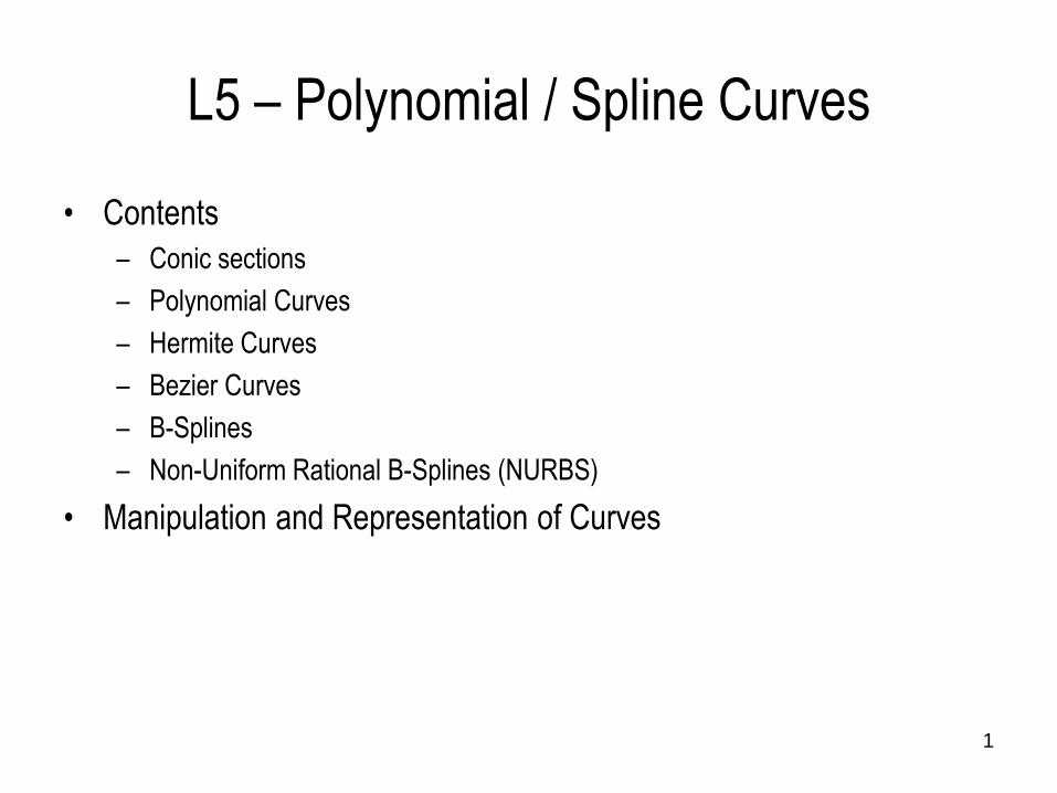
L5 – Polynomial / Spline Curves • Contents – Conic sections – Polynomial Curves – Hermite Curves – Bezier Curves – B-Splines – Non-Uniform Rational B-Splines (NURBS) • Manipulation and Representation of Curves 1
Transcript of L5 Polynomial / Spline Curves - GitHub Pages
L5 – Polynomial / Spline Curves
• Contents
– Conic sections
– Polynomial Curves
– Hermite Curves
– Bezier Curves
– B-Splines
– Non-Uniform Rational B-Splines (NURBS)
• Manipulation and Representation of Curves
1
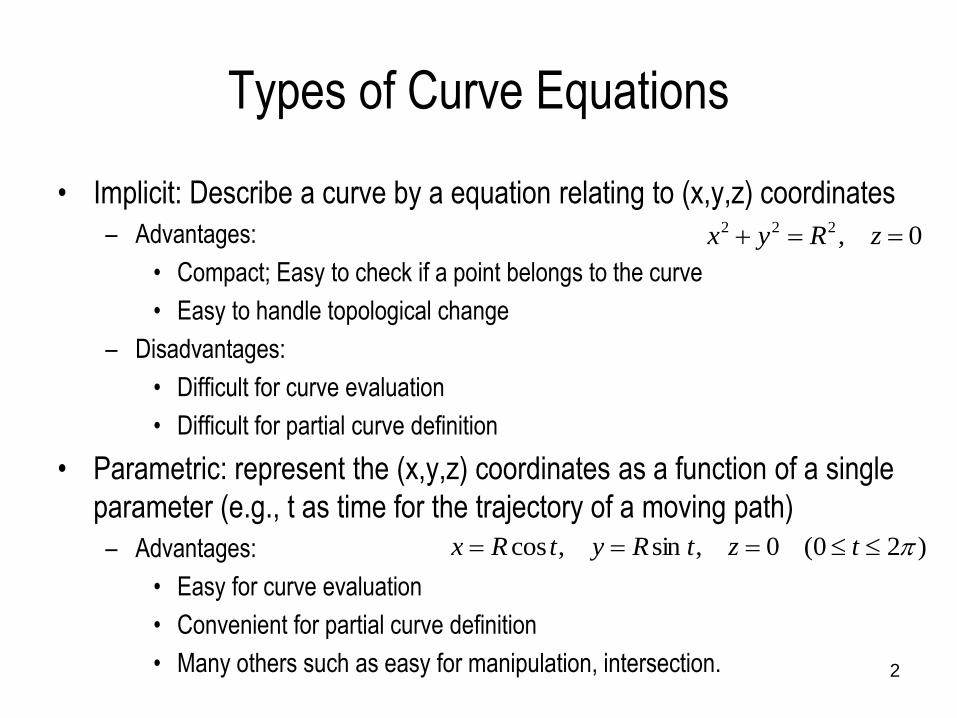
Types of Curve Equations
• Implicit: Describe a curve by a equation relating to (x,y,z) coordinates
– Advantages:
• Compact; Easy to check if a point belongs to the curve
• Easy to handle topological change
– Disadvantages:
• Difficult for curve evaluation
• Difficult for partial curve definition
• Parametric: represent the (x,y,z) coordinates as a function of a single
parameter (e.g., t as time for the trajectory of a moving path)
– Advantages:
• Easy for curve evaluation
• Convenient for partial curve definition
• Many others such as easy for manipulation, intersection. 2
0,222 zRyx
)20(0,sin,cos tztRytRx
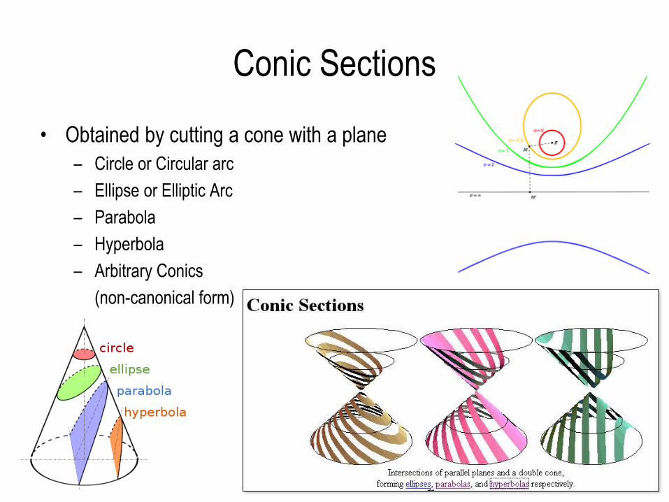
Conic Sections
• Obtained by cutting a cone with a plane
– Circle or Circular arc
– Ellipse or Elliptic Arc
– Parabola
– Hyperbola
– Arbitrary Conics
(non-canonical form)
3
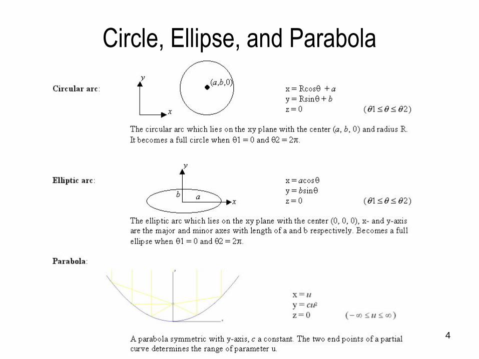
Circle, Ellipse, and Parabola
4
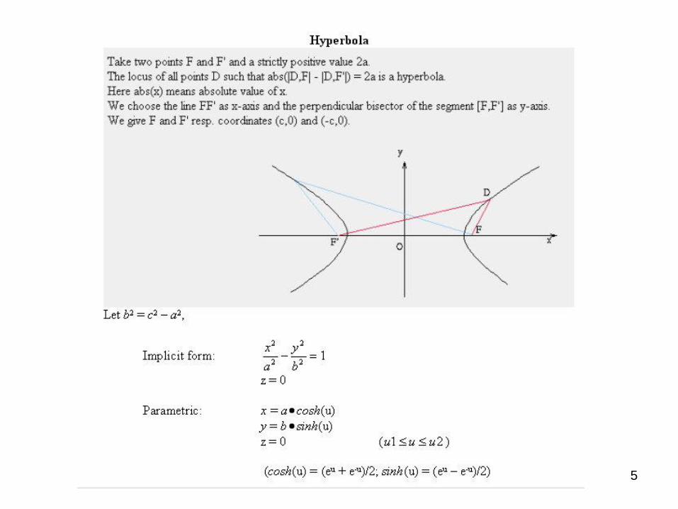
Hyperbola
5
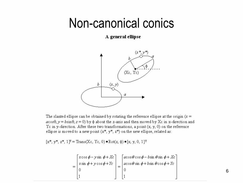
Non-canonical conics
6

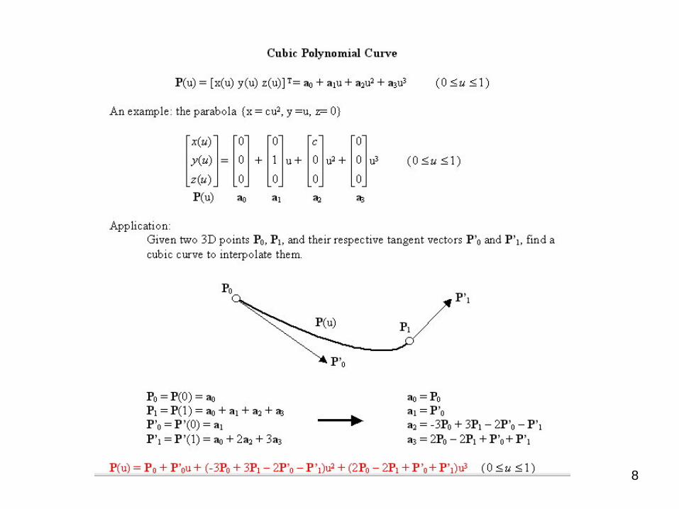
Cubic Polynomial Curve
• Definition
P(u) = [x(u) y(u) z(u)] T = a0 + a1u + a2u2 + a3u
3 (0 u 1)
• Major Drawback:
– a0, a1, a2, a3 are simply algebraic vector coefficients;
– they do not reveal any relationship with the shape of the curve itself.
– In other words, the change of the curve’s shape cannot be intuitively
anticipated from changes in their values.
• Data fitting? How?
– Parameterization (Uniform, Chordal Length)
– Least-Square Solution
• Why not quadric?
P(u) = a0 + a1u + a2u2 (0 u 1)
7
Cubic Polynomial Curve
8
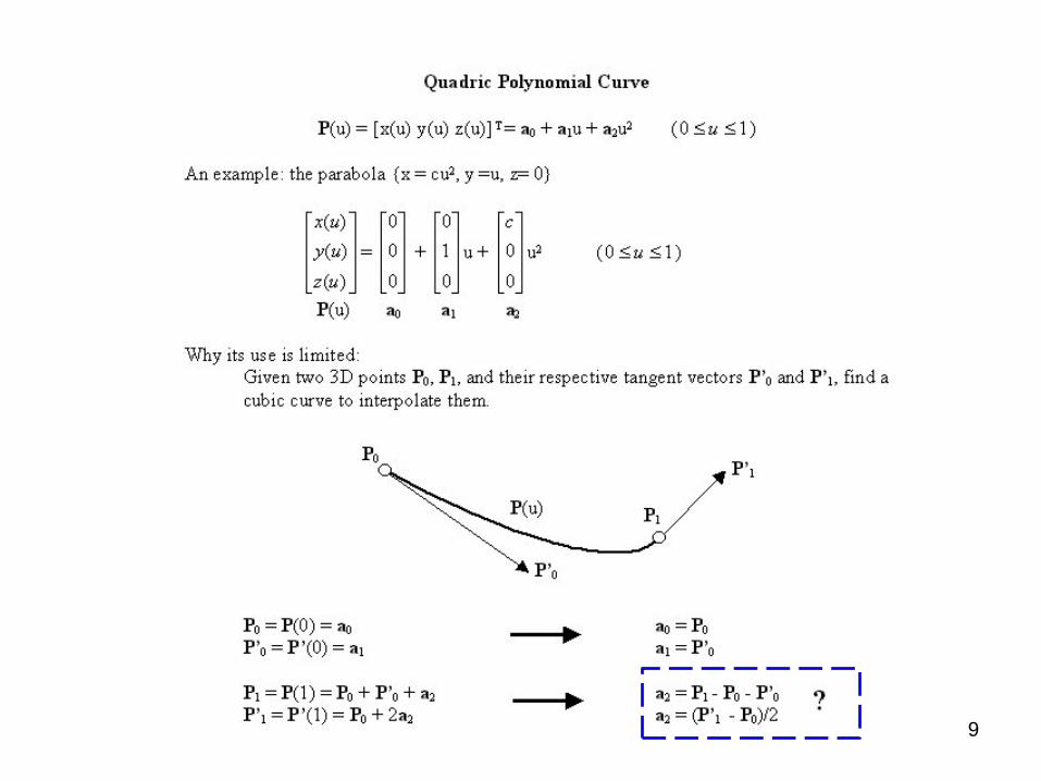
Quadric Polynomial Curve
9
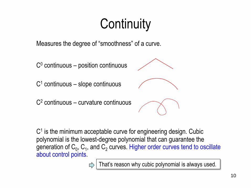
Continuity
10
Measures the degree of “smoothness” of a curve.
C0 continuous – position continuous
C1 continuous – slope continuous
C2 continuous – curvature continuous
C1 is the minimum acceptable curve for engineering design. Cubic polynomial is the lowest-degree polynomial that can guarantee the generation of C0, C1, and C2 curves. Higher order curves tend to oscillate about control points.
That’s reason why cubic polynomial is always used.
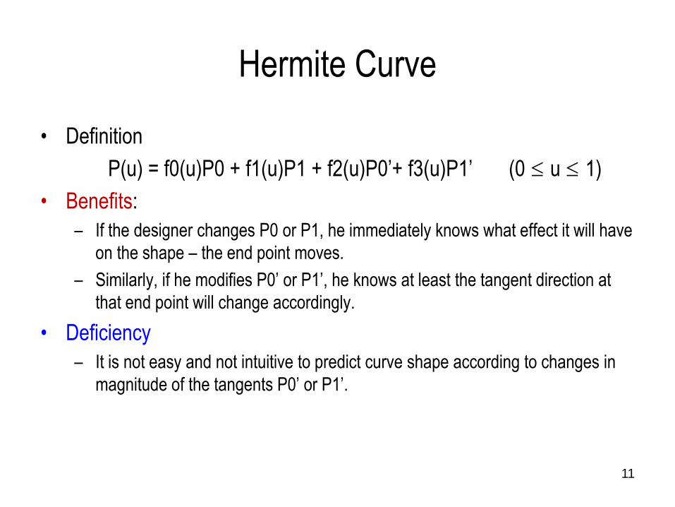
Hermite Curve
• Definition
P(u) = f0(u)P0 + f1(u)P1 + f2(u)P0’+ f3(u)P1’ (0 u 1)
• Benefits:
– If the designer changes P0 or P1, he immediately knows what effect it will have
on the shape – the end point moves.
– Similarly, if he modifies P0’ or P1’, he knows at least the tangent direction at
that end point will change accordingly.
• Deficiency
– It is not easy and not intuitive to predict curve shape according to changes in
magnitude of the tangents P0’ or P1’.
11
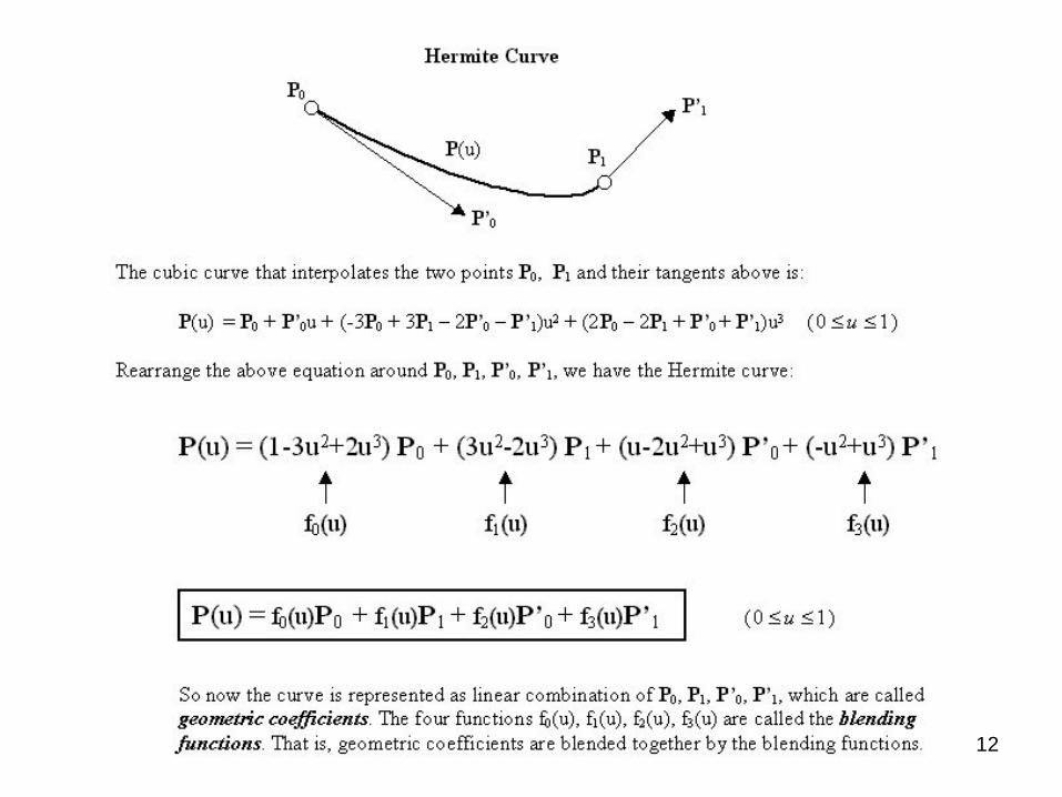
Definition of Hermite Curve
12

Effect Tangents’ Directions on a Hermite Curve
13
Change of tangent direction at point
p1
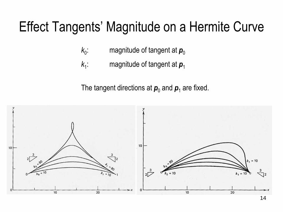
Effect Tangents’ Magnitude on a Hermite Curve
14
k0: magnitude of tangent at p0
k1: magnitude of tangent at p1
The tangent directions at p0 and p1 are fixed.
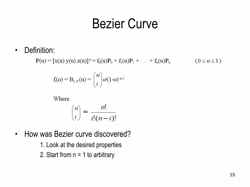
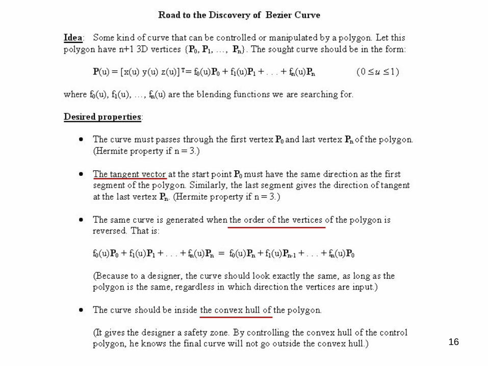
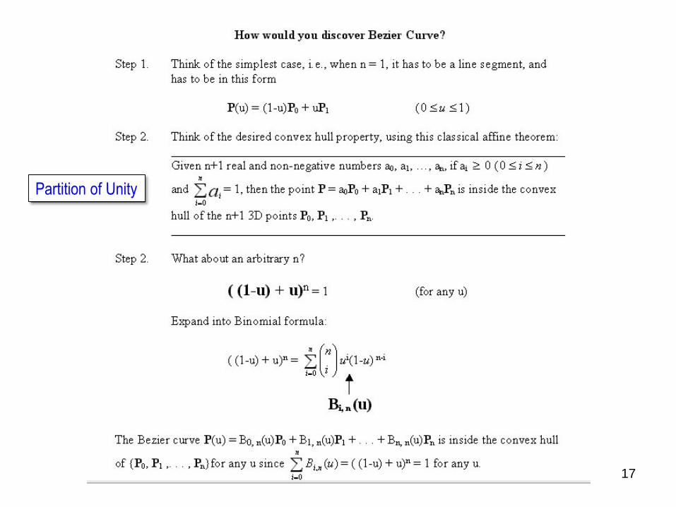
Bezier Curve
• Definition:
• How was Bezier curve discovered?
1. Look at the desired properties
2. Start from n = 1 to arbitrary
15
16
17
Partition of Unity
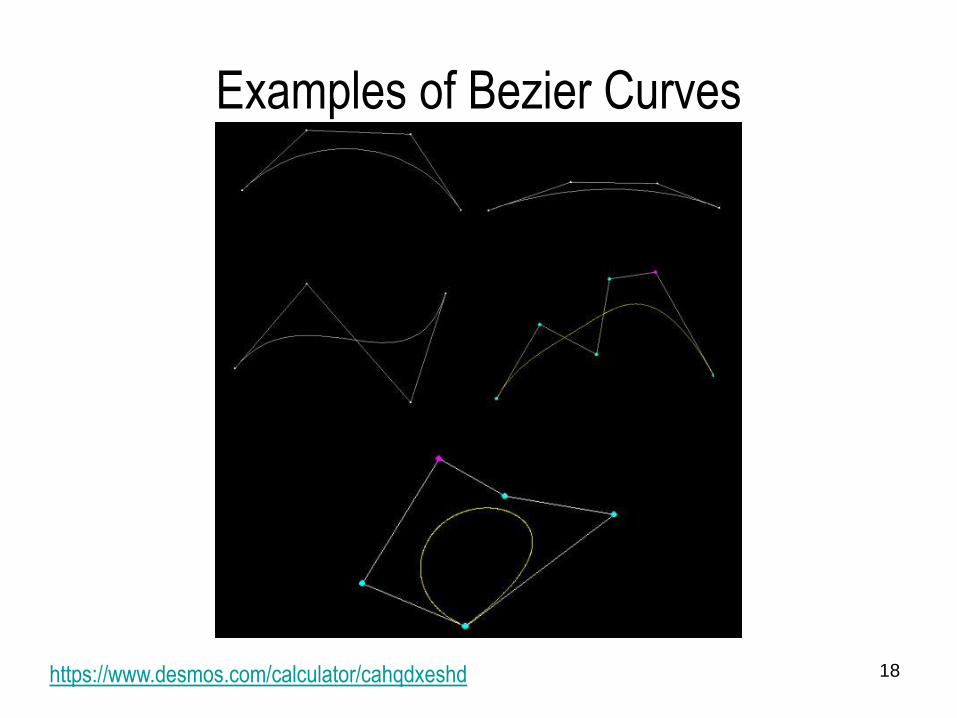
Examples of Bezier Curves
18https://www.desmos.com/calculator/cahqdxeshd
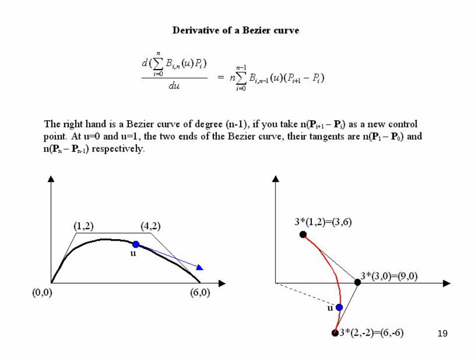
19
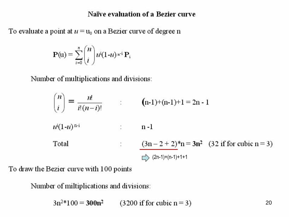
20
(2n-1)+(n-1)+1+1
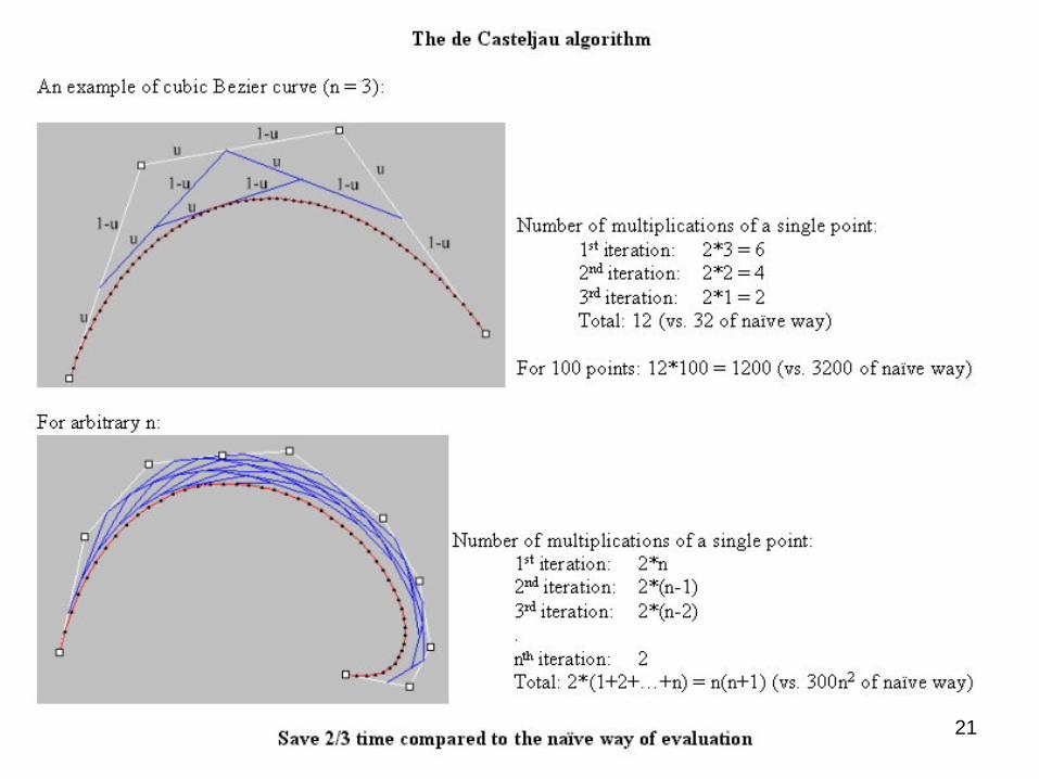
21
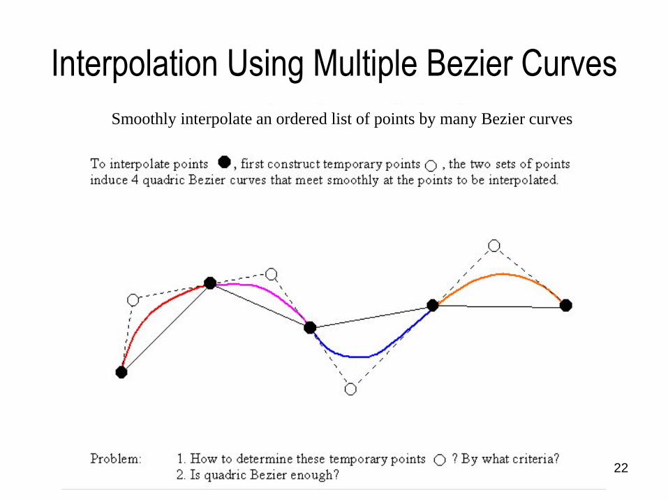
Interpolation Using Multiple Bezier Curves
22
Smoothly interpolate an ordered list of points by many Bezier curves
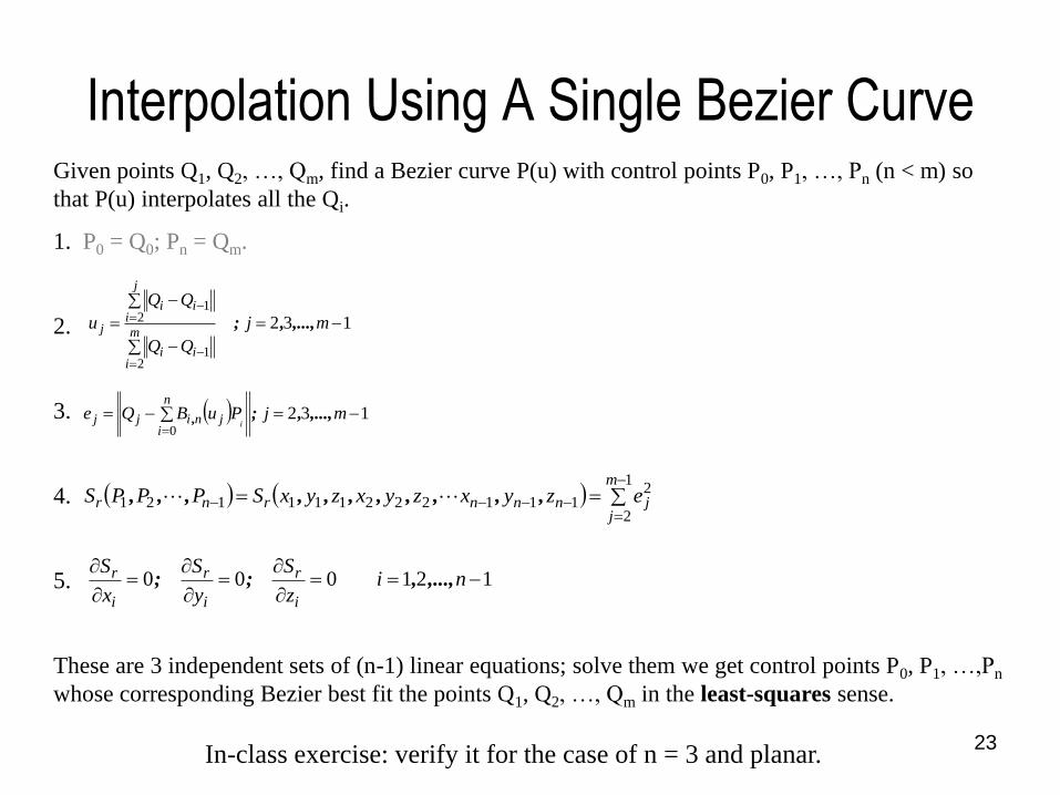
Interpolation Using A Single Bezier Curve
23
Given points Q1, Q2, …, Qm, find a Bezier curve P(u) with control points P0, P1, …, Pn (n < m) so
that P(u) interpolates all the Qi.
1. P0 = Q0; Pn = Qm.
2.
3.
4.
5.
These are 3 independent sets of (n-1) linear equations; solve them we get control points P0, P1, …,Pn
whose corresponding Bezier best fit the points Q1, Q2, …, Qm in the least-squares sense.
1320
mjPuBQen
ijnijj i
,...,,;,
132
21
21
mj
um
iii
j
iii
j ,...,,;
121000
ni
z
S
y
S
x
S
i
r
i
r
i
r ,...,,;;
1
2
2111222111121
m
jjnnnrnr ezyxzyxzyxSPPPS ,,,,,,,,,,,
In-class exercise: verify it for the case of n = 3 and planar.
Drawbacks of Bezier curve
• High degree
– The degree is determined by the number of control points which tend to be
large for complicated curves. This causes oscillation as well as increases the
computation burden.
• Non-local modification Property
– When modifying a control point, the designer wants to see the shape change
locally around the moved control point. In Bezier curve case, moving a control
point affects the shape of the entire curve, and thus the portions on the curve
not intended to change.
– http://www.mat.dtu.dk/people/J.Gravesen/cagd/bez9-3.html
• Intractable linear equations
– If we are interested in interpolation rather than just approximating a shape, we
will have to compute control points from points on the curve. This leads to
systems of linear equations, and solving such systems can be impractical when
the degree of the curve is large. 24
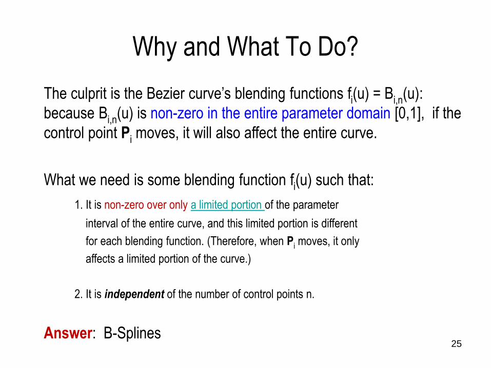
Why and What To Do?
25
The culprit is the Bezier curve’s blending functions fi(u) = Bi,n(u):
because Bi,n(u) is non-zero in the entire parameter domain [0,1], if the
control point Pi moves, it will also affect the entire curve.
What we need is some blending function fi(u) such that:
1. It is non-zero over only a limited portion of the parameter
interval of the entire curve, and this limited portion is different
for each blending function. (Therefore, when Pi moves, it only
affects a limited portion of the curve.)
2. It is independent of the number of control points n.
Answer: B-Splines
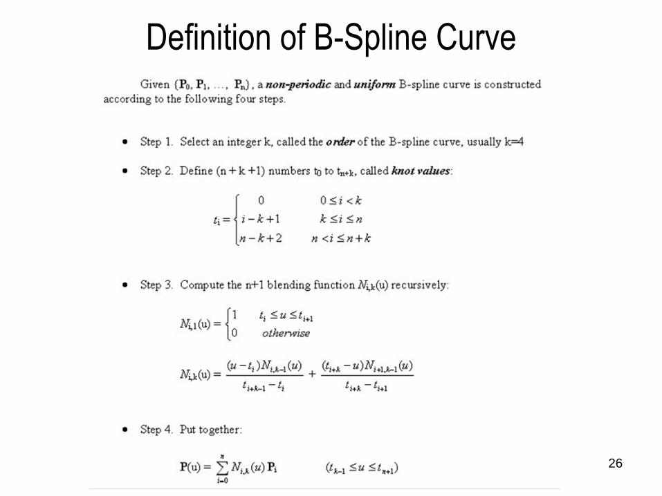
Definition of B-Spline Curve
26
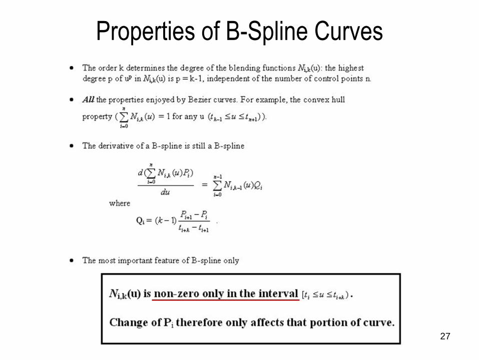
Properties of B-Spline Curves
27
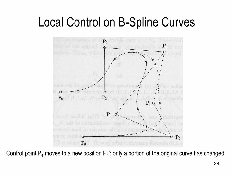
Local Control on B-Spline Curves
28
Control point P4 moves to a new position P4’; only a portion of the original curve has changed.
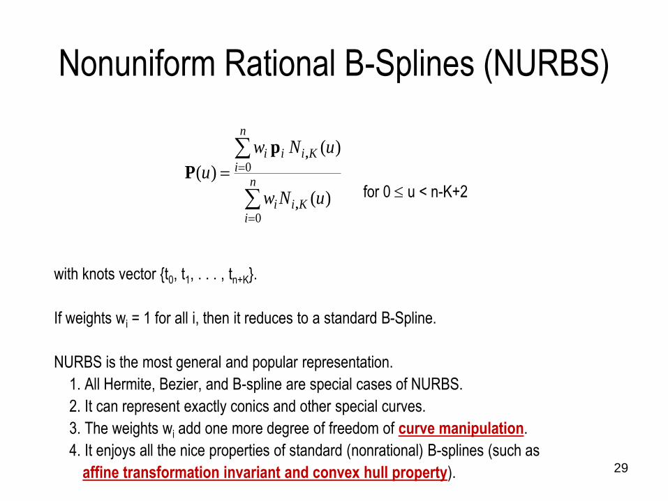
Nonuniform Rational B-Splines (NURBS)
29
for 0 u < n-K+2
with knots vector {t0, t1, . . . , tn+K}.
If weights wi = 1 for all i, then it reduces to a standard B-Spline.
NURBS is the most general and popular representation.
1. All Hermite, Bezier, and B-spline are special cases of NURBS.
2. It can represent exactly conics and other special curves.
3. The weights wi add one more degree of freedom of curve manipulation.
4. It enjoys all the nice properties of standard (nonrational) B-splines (such as
affine transformation invariant and convex hull property).
n
iKii
n
iKiii
uNw
uNw
u
0
0
)(
)(
)(
,
,p
P
30
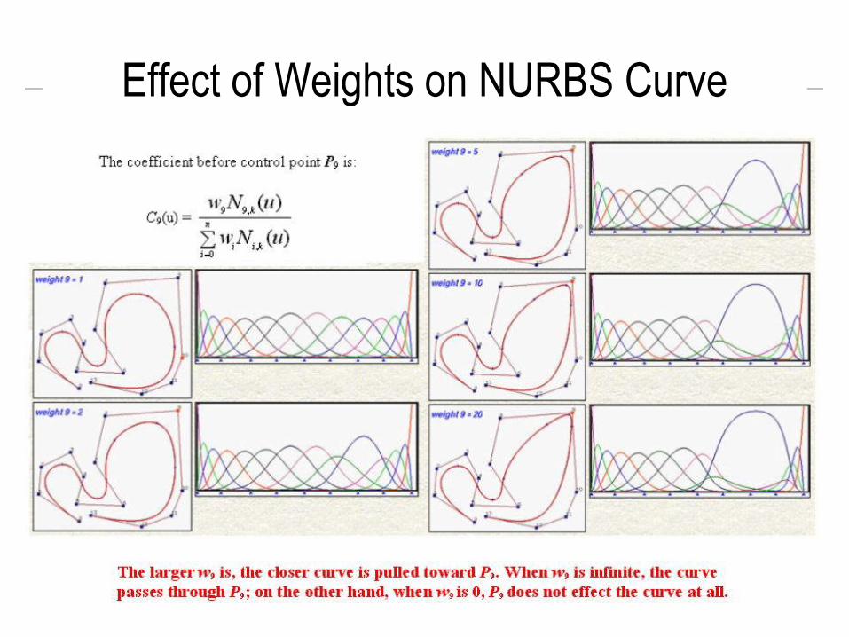
Effect of Weights on NURBS Curve
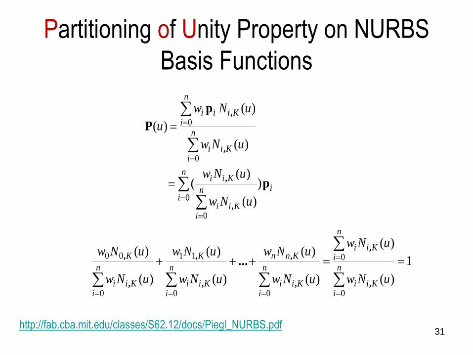
Partitioning of Unity Property on NURBS
Basis Functions
31
n
iKii
n
iKiii
uNw
uNw
u
0
0
)(
)(
)(
,
,p
P
i
n
in
iKii
Kii
uNw
uNwp
,
,
0
0
)
)(
)((
1
)(
)(
)(
)(
)(
)(
)(
)(
0
0
00
11
0
00
n
iKii
n
iKii
n
iKii
Knn
n
iKii
K
n
iKii
K
uNw
uNw
uNw
uNw
uNw
uNw
uNw
uNw
,
,
,
,
,
,
,
,...
http://fab.cba.mit.edu/classes/S62.12/docs/Piegl_NURBS.pdf

32
Take Home Questions (1)
1.
Give the parametric curve
representation of the ellipse
shown left. (Hint: utilize
transformations.)
2. Consider the Hermite curve defined in the plane with P(0) = (2,3), P(1) =
(4, 0), P’(0) = (3,2), and P’(1) = (3, -4).
a. Find a Bezier curve of degree 3 that represents this Hermite curve
as exactly as possible, i.e., decide the four control points of the
Bezier curve.
b. Expand both of the curve equations into polynomial form and
compare them. Are they identical?
33
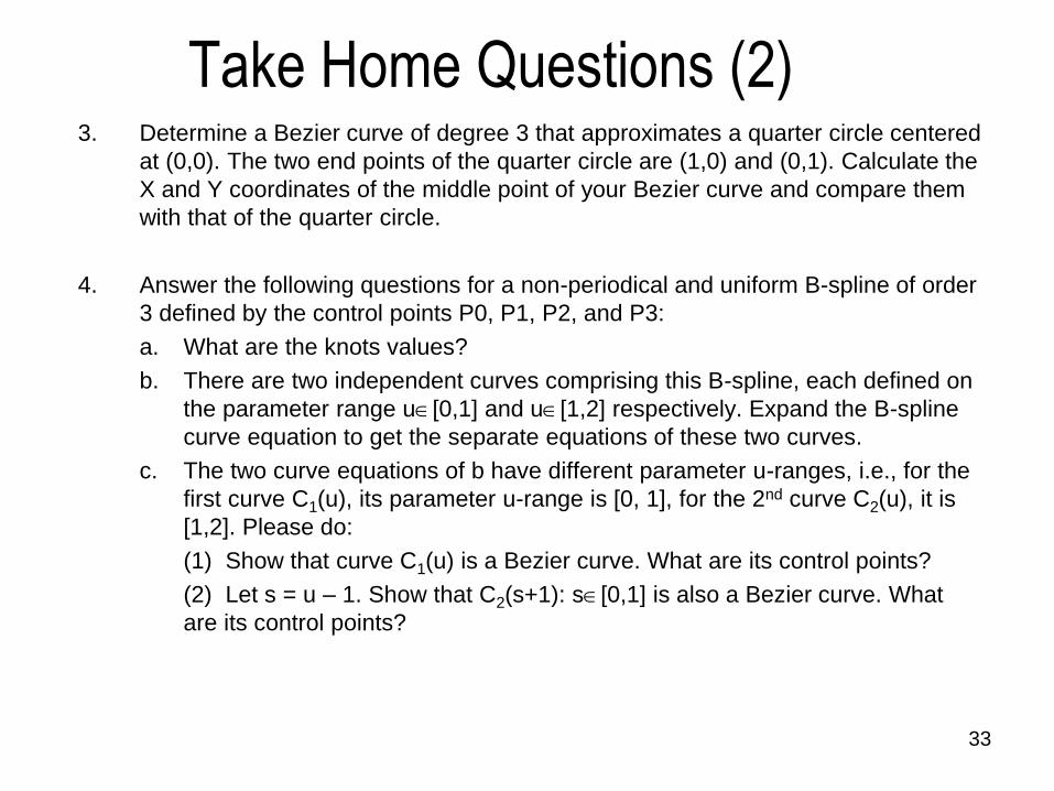
Take Home Questions (2)3. Determine a Bezier curve of degree 3 that approximates a quarter circle centered
at (0,0). The two end points of the quarter circle are (1,0) and (0,1). Calculate the
X and Y coordinates of the middle point of your Bezier curve and compare them
with that of the quarter circle.
4. Answer the following questions for a non-periodical and uniform B-spline of order
3 defined by the control points P0, P1, P2, and P3:
a. What are the knots values?
b. There are two independent curves comprising this B-spline, each defined on
the parameter range u[0,1] and u[1,2] respectively. Expand the B-spline
curve equation to get the separate equations of these two curves.
c. The two curve equations of b have different parameter u-ranges, i.e., for the
first curve C1(u), its parameter u-range is [0, 1], for the 2nd curve C2(u), it is
[1,2]. Please do:
(1) Show that curve C1(u) is a Bezier curve. What are its control points?
(2) Let s = u – 1. Show that C2(s+1): s[0,1] is also a Bezier curve. What
are its control points?


![3.4 Hermite Interpolation 3.5 Cubic Spline Interpolationzxu2/acms40390F15/Lec-3.4-5.pdf · Hermite Polynomial Definition. Suppose 𝑓𝑓∈𝐶𝐶 1 [𝑎𝑎,𝑏𝑏]. Let 𝑥𝑥](https://static.fdocuments.in/doc/165x107/5e2fc27b8791c714955aecaf/34-hermite-interpolation-35-cubic-spline-interpolation-zxu2acms40390f15lec-34-5pdf.jpg)
![arXiv:1312.6974v2 [stat.ME] 30 Apr 2014 · of related work on model-based curve clustering approaches using polynomial regression mix-tures (PRM) and spline regression mixtures (SRM)](https://static.fdocuments.in/doc/165x107/5eb45f0410e7004ce34f0865/arxiv13126974v2-statme-30-apr-2014-of-related-work-on-model-based-curve-clustering.jpg)